dSPACE DS1103 Control Workstation Tutorial and DC Motor ...ee.bradley.edu/projects/proj2009/dscntrl/Tutorial.pdf · dSPACE DS1103 Control Workstation Tutorial and DC ... to become

dSPACE DS1103 Control Workstation Tutorial and DC

Motor Speed Control

Tutorial

By

Annemarie Thomas

Advisor: Dr. Winfred Anakwa

May 11, 2009

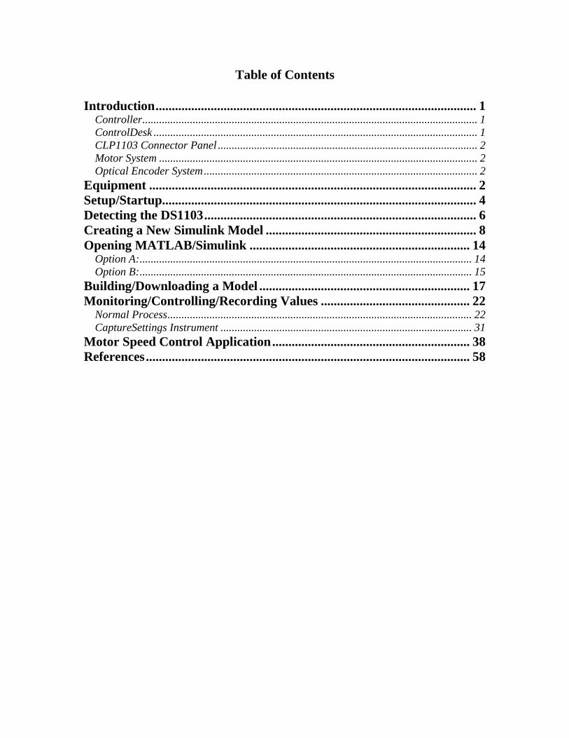
Table of Contents

Introduction ................................................................................................... 1

Controller ........................................................................................................................ 1 ControlDesk .................................................................................................................... 1 CLP1103 Connector Panel ............................................................................................. 2 Motor System .................................................................................................................. 2

Optical Encoder System .................................................................................................. 2

Equipment ..................................................................................................... 2

Setup/Startup................................................................................................. 4

Detecting the DS1103 .................................................................................... 6

Creating a New Simulink Model ................................................................. 8

Opening MATLAB/Simulink .................................................................... 14

Option A: ....................................................................................................................... 14 Option B: ....................................................................................................................... 15

Building/Downloading a Model ................................................................. 17

Monitoring/Controlling/Recording Values .............................................. 22

Normal Process ............................................................................................................. 22 CaptureSettings Instrument .......................................................................................... 31

Motor Speed Control Application ............................................................. 38

References .................................................................................................... 58

1

Introduction

The purpose of this tutorial is to introduce Bradley University’s dSPACE DS1103 Workstation

to new users. Use of this tutorial will minimize the time required for students (of senior

undergraduate level or higher) to become proficient in using the workstation. This should allow

them to spend less time learning about the workstation, so they can spend more time designing

and implementing more complex control systems.

The example system used in this tutorial is a DC motor speed control system. The controller has

been designed and simulated using both the Simulink and the dSPACE blocksets, the MATLAB-

to-DSP interface libraries, Real-Time Interface to Simulink, and Real-Time Workshop, all

located on the workstation PC. The controller will be downloaded onto the Texas Instruments’

TM320F240 DSP [1] located on the DS1103 board.

A general block diagram for the system is shown in figure 1 below.

DS1103

Motor System

ControlDesk

(Desired Speed

Input)

Load Applied to

Motor Shaft

By Brake

Optical Encoder

CLP1103

Connector

Panel

Figure 1: Motor Speed Control System Block Diagram.

Controller

The controller was designed using hand and MATLAB calculations and Simulink Simulation. It

was then added to the Simulink Model that was downloaded to the DS1103 DSP. For more

information see the final project report for this project [2].

ControlDesk

ControlDesk serves multiple purposes. It provides the interface for downloading controller

models onto the DSP and provides the ability to interface with the entire system so inputs, such

as the desired motor speed, can be altered and output data can be monitored on the PC display in

real-time.

2

CLP1103 Connector Panel

The CLP1103 Connector Panel serves as an interface between the DS1103 and all external

hardware. The CLP1103 Connector Panel contains connectors for twenty (20) Analog-to-Digital

inputs, eight (8) Digital-to-Analog outputs, and several other connectors that can be used for

Digital I/O, Slave/DSP I/O, Incremental Encoder Interfacing, CAN interfacing, and Serial

Interfacing. [3]. Only the Slave I/O (for PWM output) and Incremental Encoder interfaces are

used in this tutorial.

Motor System

The Motor System includes a motor and additional analog components, most of which are listed

in the “Equipment” section that follows.

Optical Encoder System

The Optical Encoder System is an optical encoder connected to the motor with necessary pull-up

resistors and power/ground connections added.

Equipment

Required Equipment for this tutorial is:

The dSPACE DS1103 Workstation. (See figure 2 on the next page.)

Pittman GM9236C534-R2 DC Motor.

HEDS 9100 Two Channel Optical Incremental Encoder Module and 512 CPR code

wheel (attached to the internal motor shaft).

Magtrol HB-420 Brake.

TIP120 Transistor.

IN4004 Diode.

SN7407 Hex Inverters.

Connectors with wires for the pins used as inputs and outputs to the CLP1103

Connector Panel. (See more details in the “Motor Speed Control Application”

section.)

Other required/desired electronic components (resistors and wires), power supplies,

and measurement devices.

All of this equipment was readily available at Bradley University at the time this tutorial was

written.

Note1: The next several sections are general processes that should be followed. Skip to the

section titled “Motor Speed Control Application” to follow these steps in an actual application.

Even if the example application is not being used, reading through the instructions in that section

may provide some additional hints and tips that might make using the system easier.

3

Figure 2: Workstation

Note2: If additional information is required, please refer to the final project report for this project

[2] or contact Dr. Anakwa at Bradley University.

4

Setup/Startup

1. Turn on the DS1103 Board using the power switch on the back of the expansion box.

Figure 3: Back View of Expansion Box with switch highlighted.

2. Open ControlDesk from the Start Menu.

To open ControlDesk go to: Start EE Applications dSPACE Tools ControlDesk

Figure 4: Location of ControlDesk Icon in the Start Menu

5

3. Scroll to the bottom of the ControlDesk Disclaimer dialog box when it appears and select

“Accept”.

Figure 5: ControlDesk Disclaimer dialog box.

Note: This disclaimer does not affect this workstation since the PC is currently running the

Windows XP operating system, not Windows Vista.

4. ControlDesk should now be open.

Figure 6: ControlDesk Window

Note: ControlDesk will complain if the DS1103 board is not turned on first.

6

Detecting the DS1103

Note: These steps should not need to be followed every time the system is used. These steps are

generally needed the first time the workstation is setup and any time after when an error occurs

in MATLAB when code is being built announces that the board has not been detected or the

“ds1103” and “Slave DSP” do not appear in the “Platform” tab in ControlDesk.

Figure 7: View of Platform tab in ControlDesk before and after DS1103 has been detected.

1. Select “Register” from the menu in ControlDesk.

To select “Register”, in the main menu go to: Platform Initialization Register

Figure 8: Location of Register selection in ControlDesk main menu.

7

2. From the “Register Board” dialog box that appears, select “DS1103 PPC Controller Board”

from the “Type” dropdown menu and set the “Port address” to 300. Then select the

“Register” button.

Figure 9: Correct selections in Register Board dialog box.

3. The DS1103 Board and DSP should now be reported as detected in the ControlDesk

“Platform” tab.

Figure 10: DS1103 and Slave DSP shown in the Platform tab with the system stopped.

8

Creating a New Simulink Model

For best results, a new Simulink Model should be opened from ControlDesk itself. If other

processes are used to create a new Simulink Model, there is a chance that there will be issues

when the steps in the “Building/Downloading Model” section later in this document are

followed. Once the model is created, the instructions in the “Opening MATLAB/Simulink”

section can be used to re-open, edit, and build the model in the future.

1. Create a folder on the Desktop or another location on the computer for your project.

9

2. Open ControlDesk and Select the “Platform” tab of the left menu window.

Note: Do not close ControlDesk until all the steps in this section of the tutorial are

completed.

Figure 11: Location of Platform tab in ControlDesk.

10

3. In the “Platform” window, Right-click “Simulink” and Select “New Model…” from the

menu that appears.

Figure 12: Creating a New Model from ControlDesk.

11

4. Select the folder that was created for the project from the “Look in:” drop down menu at the

top of the “New Model” window. Type in a name for the new Simulink Model file in the

“File Name:” box, and then, Select the “Open” button.

Figure 13: Naming the new Simulink Model File.

12

5. Locate the Simulink Model that opened with the name entered in the previous step and Build

it.

To Build the Model from the model’s main menu go to:

Tools Real-Time Workshop Build Model

Figure 14: Selecting Build Model.

Note: To see the Build process running, view the MATLAB “Command Window”.

13

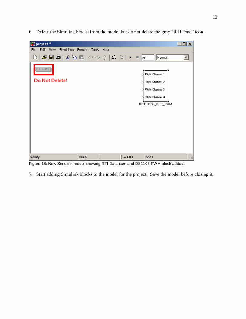
6. Delete the Simulink blocks from the model but do not delete the grey “RTI Data” icon.

Figure 15: New Simulink model showing RTI Data icon and DS1103 PWM block added.

7. Start adding Simulink blocks to the model for the project. Save the model before closing it.

14

Opening MATLAB/Simulink

There are Several Ways to open MATLAB and Simulink when a Simulink model has already

been created. Two possible options are listed below.

Option A:

Open the existing “.mdl” file for the project from its folder on the drive.

Note: This only works if you have an existing model.

1. Find the .mdl file on the drive and double-click the file to open it. (This will cause

both MATLAB and Simulink to open.)

Figure 16: test.mdl file selected to be opened.

2. Select the “RTI1103” button in the “Select dSPACE RTI Platform Support” dialog

box that appears in MATLAB.

Figure 17: Select dSPACE RTI Platform Support dialog box.

15

Option B:

Open MATLAB from ControlDesk. This process does require more steps.

1. From ControlDesk, right-click “Simulink” in the “Platform” tab, and select “Open

MATLAB”. (This will open just a MATLAB Command Window.)

Figure 18: Link to Open MATLAB from ControlDesk.

2. To open the Simulink Library Browser, enter “simulink” into the MATLAB

Command Window.

Figure 19: Enter "simulink" into the MATLAB Command Window.

16

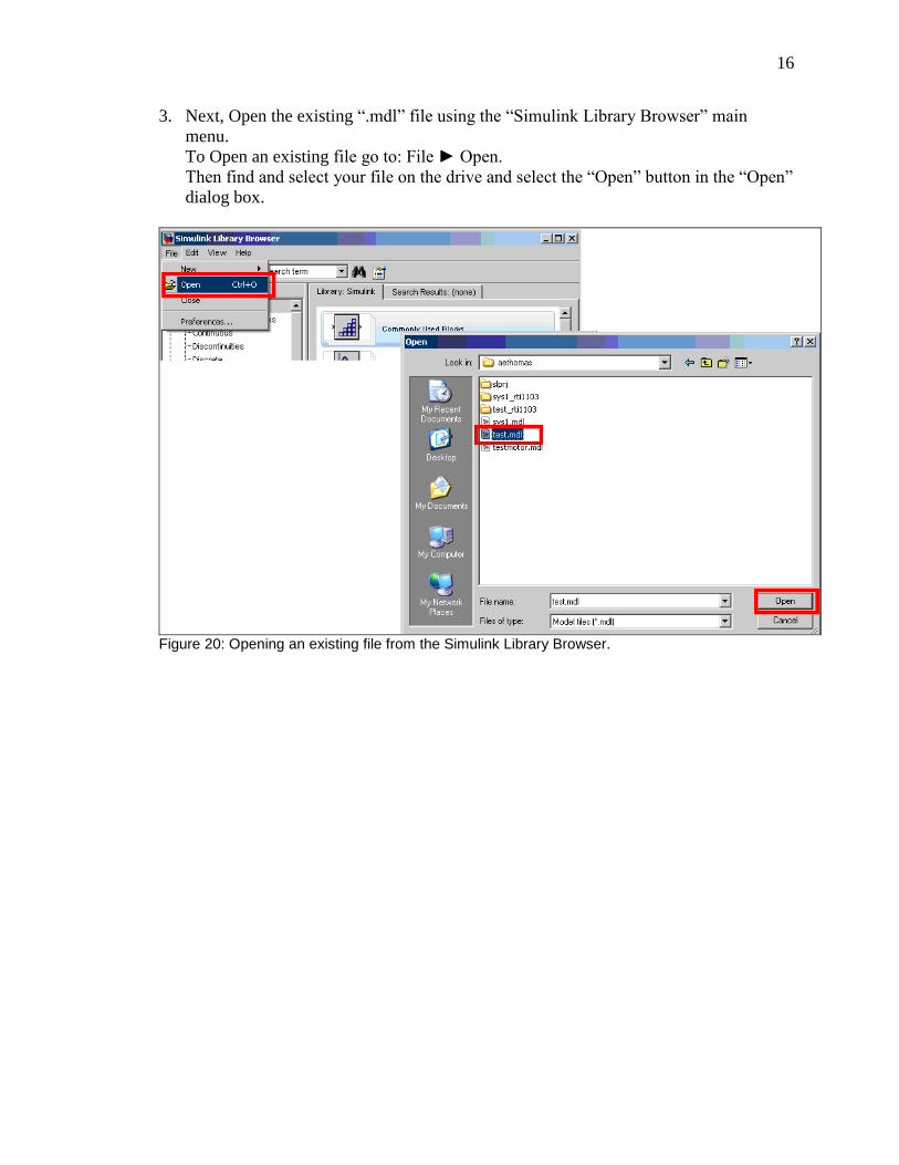
3. Next, Open the existing “.mdl” file using the “Simulink Library Browser” main

menu.

To Open an existing file go to: File Open.

Then find and select your file on the drive and select the “Open” button in the “Open”

dialog box.

Figure 20: Opening an existing file from the Simulink Library Browser.

17

Building/Downloading a Model

1. Open the “Configuration Parameters” window from the main menu of your open model

window.

To open the “Configuration Parameters” window go to:

Simulation Configuration Parameters…

Figure 21: Opening the Configuration Parameters window.

18

2. Set the required/desired parameters in the “Configuration Parameters” window. Make sure

to set the sampling time (“Fixed-step size”) to the correct value for the project.

To change the sampling time go to: Solver Fixed-step size.

Then, Set to desired sampling time.

Figure 22: Configuration Parameters window with sampling time set to 0.001s or 1ms.

19

3. Set the “Real-Time Workshop” settings and select the “Build” button to build and download

code from the Simulink model. (Code building progress is output to the MATLAB

Command Window.)

Real-Time Workshop Settings:

a. System target file: rti1103.tlc

b. Language: C

c. Make command: make_rti

d. Template makefile: rti1103.tmf

e. Select checkbox for “Generate makefile”

Note1: ControlDesk needs to be open for this step to complete all processes well. There will be

no error message if ControlDesk is not open, but certain tabs in ControlDesk used for monitoring

and controlling variables will not be automatically opened.

Figure 23: Real-Time Workshop Settings.

20

Figure 24: End of output in MATLAB Command Window for a successful build.

21

Note2: To make sure the files generated are placed in the folder desired, it is advisable to select

the “File Selector” tab at the bottom of the ControlDesk window, select and right-click the folder

where the files should be placed, and select “Change to Working Directory” before building any

code each time.

Figure 25: Setting the Working Directory/Build folder.

4. The code should be built and downloaded and running on the DS1103 and Slave DSP now.

22

Monitoring/Controlling/Recording Values

Layouts are one of the more interesting functions in ControlDesk. They allow the value of

constant/input blocks, gain blocks, and perhaps some other blocks to from the Simulink model

downloaded to the DS1103 to be changed while the system is running. They also allow real-time

reporting of output values and saving/recording of values over a time period for analysis/viewing

in MATLAB later.

Normal Process

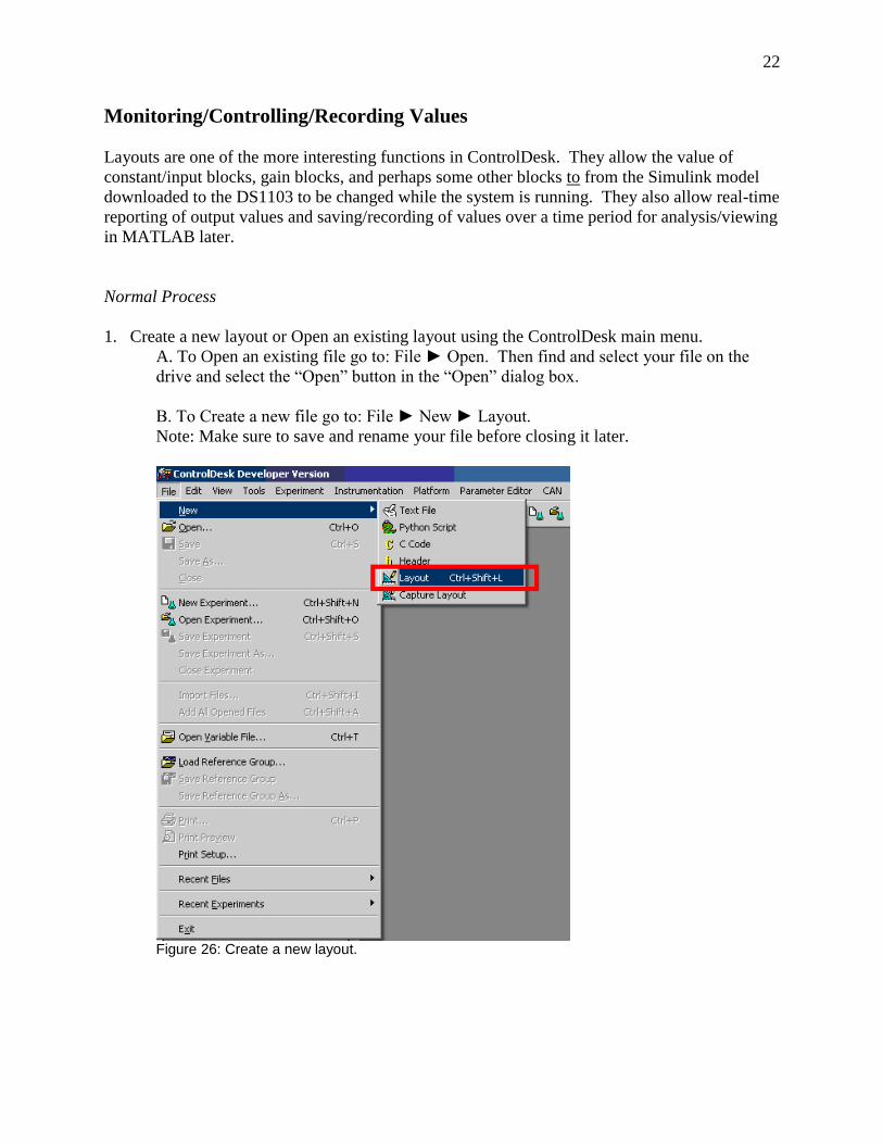
1. Create a new layout or Open an existing layout using the ControlDesk main menu.

A. To Open an existing file go to: File Open. Then find and select your file on the

drive and select the “Open” button in the “Open” dialog box.

B. To Create a new file go to: File New Layout.

Note: Make sure to save and rename your file before closing it later.

Figure 26: Create a new layout.

23

2. Expand the layout window that appears in the ControlDesk workspace to fit most of the

workspace by dragging the double-headed arrows that appear when the mouse passes over

the edges of the window.

Figure 27: Expanded layout window in ControlDesk.

3. Set ControlDesk to “Edit Mode” by either selecting it from the toolbar or by selecting it from

the “Instrumentation” dropdown menu of the main menu. (The “Virtual Instruments” side

panel should appear.)

Figure 28: Selecting Edit Mode in ControlDesk.

24

4. Now “Virtual Instruments” and “Data Acquisition” Tools can be added to the layout. This is

done by single-clicking instruments in the side panel (without holding the mouse button

down), then clicking and then holding the mouse button down in the layout window while

dragging the corner of the box that begins to appear for that particular instrument.

Figure 29: Adding a Virtual Instrument.

25

Figure 30: Adding Plotter Array from the Data Acquisition Menu.

26

5. Verify a tab for the “.sdf” file generated for the project is available near the bottom of the

ControlDesk window. If it is not, rebuild the project using the instructions in the

“Building/Downloading a Model” section of this tutorial, beginning on page 13.

Figure 31: Location of .sdf tab in the ControlDesk window.

27

6. To connect/assign variables from the Simulink model downloaded to the DS1103, locate the

variable in the “.sdf” menu(s) and then click-and-drag it to its instrument in the layout.

(Generally, the values of constants and gain blocks in the model can be monitored and

modified/controlled in real-time and outputs/connections between blocks can be monitored

only.)

Note: To connect to the outputs of dSPACE blocks in the downloaded Simulink model, a gain

(of 1) block needs to be connected to the output of the block if nothing else is connected to it

other than a terminator block.

Figure 32: Connecting Variables to Instruments.

28

Figure 33: Completed layout with location of additional connections not shown in Figure 28 highlighted.

29

7. Change the properties of the instruments as desired.

Accessing the “Properties” menu(s) for a particular instrument done by either:

A. Left-clicking the instrument to select it and then selecting “Properties” from the

ControlDesk main menu “View” menu.

B. Right-clicking the instrument and selecting “Properties”.

Figure 34: Two methods of opening the Properties dialog for an instrument.

Find the property that should change under one of the tabs and change it. (Generally, only

Max and Min “Range” values need to be changed and/or Range “Check Mode” needs to be

Enabled, but other properties such as the color of the instrument and text can be changed as

well.)

Figure 35: Changing the Range of the DutyCycle Slider input.

30

8. Verify the instruments now functions as desired without affecting the system (or the other

instruments) using “Test Mode”, which is found in a similar manner to “Edit Mode” in Step

3 of this section. (This is useful to verify that the “Range” enabled for “Check Mode” for an

instrument such as the “NumericInput” instrument - not used in this section - rejects values

input that are outside that range.)

Figure 36: Location of Test Mode button on main toolbar.

9. To use the instruments to control and monitor that actual, running, real-time system, select

“Animation Mode” in a similar manner to selecting “Edit Mode” in Step 3 of this section. (It

appears “Properties” can also be modified in this mode.)

Figure 37: System running with Animation Mode active.

10. Additional instruments such as the “CaptureSettings” instrument, used for saving/recording

data, can be added later by repeating Steps 3-9 of this section for the new instrument. It

should also be possible to create and use multiple layouts at the same time.

Note: For instructions/details about the “CaptureSettings” instrument, see the “CaptureSettings

Instrument” subsection that follows.

31

CaptureSettings Instrument

The “CaptureSettings” instrument found in the “Data Acquisition” instrument menu allows data

output on “PlotterArray” instruments (and only “PlotterArray” instruments) to be saved/recorded

for later analysis/use in MATLAB or perhaps some other program.

Figure 38: CaptureSettings instrument (red boxes) added to a layout with associated PlotterArrays (blue boxes). A NumericInput instrument is also included in this layout below the slider.

32

The “CaptureSettings” instrument is added in the same way as any other instrument (See Steps

3-9 in the “Normal Process” subsection previous to this one.), but the space provided for it must

be large enough to access all its functions and most of the “Properties” can also be accessed

using the ”Settings…” button on the instrument.

Figure 39: Most tabs in the Properties and Settings dialog boxes for the CaptureSettings instrument are exactly the same.

Note: For this tutorial only the “Stream to Disk” “Acquisition” method was used in its simplest

form. To see more functions of this instrument, search for “How to Generate and Save

Reference Data” or “Working with Data Captures” in the ControlDesk “Help” menu found on

the ControlDesk main menu bar.

After the CaptureSettings instrument has been added and PlotterArrays have been added for the

variables that should be recorded:

1. Set the top dropdown menu for the instrument is to “PPC - HostService”. (The name for the

project will be included as well.)

2. Open the Settings or Properties dialog for the CaptureSettings Instrument and select the

“Acquisition” tab. Select the bullet box for “Stream to Disk”.

33

3. Select the button with “…” at the end of the line for “Stream to Disk” and create or select a

file for the data to be saved to. The file will be saved as an “.idf” file.

Figure 40: Set Stream to Disk mode and create/select location for captured data.

4. Select “OK” at the bottom of the dialog box to exit the menu.

5. If the “Start” button on the instrument is selected now, ControlDesk may report an error with

the “Length” or “Downsampling” Settings. Arbitrarily setting the “Length” to “2” will fix

this for the example application.

Figure 41: Setting the Length for the capture to 2 seconds.

34

6. Select “Start” on the instrument to start saving data, and then Select “Stop” when the desired

data capture is completed.

Figure 42: Saving data.

Note: This will overwrite any data stored previously in the “.idf” file created earlier. If the data

should not be rewritten follow Steps 1-2 again between captures an Create/Select a “.idf” file

with a different name.

7. Convert the “.idf” file to a MATLAB “.mat” file by Selecting “Convert IDF File…” from the

“Tools” menu on the ControlDesk main menu, and then Selecting the “.idf” file containing

the saved data and Selecting/Creating the “.mat” file the converted data should be saved to

using the “Source File” and “Destination File(s)” “…” buttons and Selecting the “Convert”

button.

Figure 43: Converting an .idf file to a .mat file.

35

8. Open the “.mat” file from the location it was saved to on the drive.

Figure 44: Open the .mat file.

9. Select the “Finish’ button from the MATLAB “Import Wizard” dialog box that opens.

Figure 45: MATLAB Import Wizard dialog box.

36

10. From the MATLAB “Workspace”, Double-click (or Right-click and Select “Open

Selection”) the structure with the same name as the “.mat” file to open the “Variable Editor”

for the file.

11. Plot the data (or manipulate it in some other manner).

The “X” structure contains the time values in its “Data” array.

The values for the variables that were recorded are found in the “Data” arrays for each

“<1x1 struct>” of the “Y” structure. To determine which variable is found in each “<1x1

struct>” of “Y”, Double-click the structure to open it and look at the “Value” of its

“Name” label. (See figure 47 on next page.)

The full identifying label for each variable can be found at the top of the “Variable

Editor” window when it is open.

Example MATLAB code to plot both variables from the figures in this section on the

same plot: >> plot(data_5_6.X.Data, data_5_6.Y(1,1).Data) %in or RPM_in

>> hold on

>> plot(data_5_6.X.Data, data_5_6.Y(1,2).Data) %out or RPM_out

>> hold off

(Plot shown in figure 46 on the next page.)

37

0 0.5 1 1.5 2 2.5 3 3.5 4 4.5 5-200

-100

0

100

200

300

400

500

X=Time(s)

Y=

Speed(R

PM

)

in

out

Figure 46: Example data plotted in MATLAB with labels/color added manually.

Figure 47: Locating the Data for the RPM_in variable. (RPM_out was in data_5_6.Y(1,2).)

38

Motor Speed Control Application

1. Construct the motor subsystem shown in the figure below, also connecting the optical

encoder and code wheel to the internal motor shaft and adding the brake. Also add the 5 Volt

power connection and the 2.7 kΩ pull-up resistors between 5 Volts and the encoder channels,

A and B. Verify 5 Volt and 25 Volt DC power supplies are set correctly before connecting to

the system.

Figure 48: Motor Hardware Schematic.

For the motor-optical encoder system provided at Bradley University, the motor and optical

encoder connections are shown in the figure on the next page. The pin assignment for the

TIP120 NPN transistor is shown in the figure below.

39

Figure 49: TIP120 NPN transistor pin assignment.

Figure 50: Motor and encoder connections for system at Bradley University.

40

2. Make all connections between the Connector Panel, the encoder and the Motor System. The

required connections to the Slave I/O and Inc1 connectors are shown in the figures that

follow.

Note: Colors listed are for the wires used on the current version of the connectors at Bradley

University.

Figure 51: PWM connections on Slave I/O connector.

Figure 52: Encoder Connections to/from Inc1 connector.

Note: Once code has been downloaded at later steps of these instructions, it is generally best

to turn the power supplies on after downloading the code and turn them off before stopping

the code from running in ControlDesk.

41

3. Now that all the hardware connections are complete, the work with ControlDesk and

Simulink can begin. Start by following the instructions in the sections of this tutorial labeled:

a. Setup/Startup

b. Detecting the DS1103

c. Creating a New Simulink Model

Leave the model open after saving it or re-open it using the instructions in the “Opening

MATLAB/Simulink” section.

4. Now, Add the DS1103 dSPACE blocks needed for PWM generation and Encoder input

capture can be added. These blocks are found in the “Simulink Library Browser” under the

“dSPACE RTI1103” heading on the left menu window.

Figure 53: Location of dSPACE DS1103 blocks in the Simulink Library Browser.

42

4a. Locate the PWM block labeled “DS1103SL_DSP_PWM” at:

dSPACE RTI1103 DS1103 SLAVE DSP DS1103SL_DSP_PWM.

Click and Drag the block into the model created for the project.

Figure 54: Locating and Adding the PWM block.

43

4b. Some features such as the encoder blocks require more than one block to function. One

block has outputs. The other block is for more general settings that would also apply to other

related (encoder) blocks if they were used.

Locate the Encoder blocks labeled “DS1103ENC_SETUP” and “DS1103ENC_POS_C1” at:

dSPACE RTI1103 DS1103 MASTER PPC DS1103ENC_SETUP.

And

dSPACE RTI1103 DS1103 MASTER PPC DS1103ENC_POS_C1.

Click and Drag both blocks into the model created for the project.

Figure 55: Locating and Adding the encoder blocks.

44

5. Add and Connect constant, gain, terminator, and ground blocks to the Simulink project then

save the project, but do not close it.

a. Add a constant block and connect it to “PWM Channel 1” of the PWM block. Set its

value to a number between 0 and 1. Change the label of the block to “DutyCycle”.

(This is the range for the input to the block as a percentage (0.5 = 50%) of the duty

cycle.)

b. Connect gain blocks to “Enc position” and “Enc delta position”. Set the gain of these

blocks to “1”. Label the connections going into or out of these blocks “Enc1” and

“Enc2”. (If these gain blocks are not added at this point, the outputs will probably not

be monitorable in ControlDesk later.)

c. Connect the “PWM Channel 2”, “PWM Channel 3”, and “PWM Channel 4” inputs to

the PWM block to ground since they are not being used in this project. (Any

connections that are open need to be attached to either a terminator or ground.)

d. Connect the output of the gain blocks to terminator blocks.

Figure 56: Simulink model after adding blocks and connections and saving. The DutyCycle is set to 50%.

45

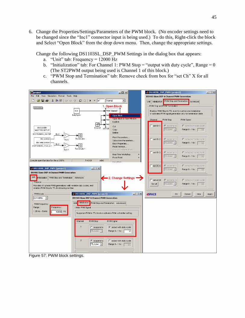
6. Change the Properties/Settings/Parameters of the PWM block. (No encoder settings need to

be changed since the “Inc1” connector input is being used.) To do this, Right-click the block

and Select “Open Block” from the drop down menu. Then, change the appropriate settings.

Change the following DS1103SL_DSP_PWM Settings in the dialog box that appears:

a. “Unit” tab: Frequency = 12000 Hz

b. “Initialization” tab: For Channel 1: PWM Stop = “output with duty cycle”, Range = 0

(The ST2PWM output being used is Channel 1 of this block.)

c. “PWM Stop and Termination” tab: Remove check from box for “set Ch” X for all

channels.

Figure 57: PWM block settings.

46

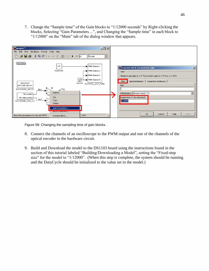
7. Change the “Sample time” of the Gain blocks to “1/12000 seconds” by Right-clicking the

blocks, Selecting “Gain Parameters…”, and Changing the “Sample time” in each block to

“1/12000” on the “Main” tab of the dialog window that appears.

Figure 58: Changing the sampling time of gain blocks.

8. Connect the channels of an oscilloscope to the PWM output and one of the channels of the

optical encoder in the hardware circuit.

9. Build and Download the model to the DS1103 board using the instructions found in the

section of this tutorial labeled “Building/Downloading a Model”, setting the “Fixed-step

size” for the model to “1/12000”. (When this step is complete, the system should be running

and the DutyCycle should be initialized to the value set in the model.)

47

10. Now, it is time to have some fun with ControlDesk. Create a layout in ControlDesk

following the directions in the “Monitoring/Controlling/Recording Values” section of this

tutorial. Connect the following variables/values to the type of instrument(s) indicated.

a. DutyCycle: Slider (Change Max Range to “1”) and Display and PlotterArray

b. Enc1: Display

c. Enc2: Display

Figure 59: Layout in ControlDesk with system running and slider used to change the DutyCycle.

11. Observe that changing the DutyCycle value using the slider changes the duty cycle of the

PWM measurement on the oscilloscope to a similar percentage and changes the encoder

frequency observed. Also observe that the DutyCycle has approximately a 12 kHz frequency

using the oscilloscope.

12. Observe that in the case of this system, the absolute value of the Enc1 output on the

ControlDesk Layout generally increases since the motor shaft is only rotating in one

direction and it is probably measuring distance. Multiplying the Enc2 output on the

ControlDesk Layout by the inverse of the sampling time (the frequency), 12000 in this case

should approximately correspond to the Encoder frequency reported on the oscilloscope.

48

13. Now, Delete the instruments from the ControlDesk layout and save it. Also, Delete the

“DutyCycle” and “Gain” blocks from the Simulink model, Delete the “Enc1” label, and

reconnect the “Enc position” output to its terminator block. Save the model.

Figure 60: Simulink model after Step 13 is completed.

49

14. Setup/Add the blocks to the Simulink model for the RPM output calculation/conversion.

a. Re-label the “Enc delta position” output connection “count_out”.

b. Add another gain block between “Gain1” and the terminator block.

c. Label these two gain blocks “count_to_Hz” and “Hz_to_RPM” and set the sample

time for each block to “1/12000” (See Step 7 in this section).

d. Change the gain of the “count_to_Hz” block to “12000” and of the “Hz_to_RPM”

block to “0.019881”.

e. Label the connection between the two gain blocks “Hz” and between the second gain

block and the terminator “RPM_out”. (RPM_out is the actual output for the system.)

Note: Leave enough space between the encoder block output and the first gain block for an

additional connection in the upward direction later.)


50

15. Add the desired RPM input block and conversion blocks.

a. Add a Constant block and two (2) Gain blocks toward the top on the Simulink model.

b. Label the constant block “RPM_in” and change its gain to “0”.

c. Connect the two gain blocks to the output of the “RPM_in” block in series with one

another.

d. Label the first Gain block “RPM_to_Hz” and the second Gain block “Hz_to_count”

and set the sample time for both blocks to “1/12000”.

e. Change the gain of the “RPM_to_Hz” block to “50.2996” and of the “Hz_to_count”

block to “”, and label the connection between the two gain blocks “Hz”.

Note: It will be necessary to increase the size of the window for the model and rearrange

some blocks to fit all the blocks in the model at this step or at some point later in the process.


51

16. Add a Sum block with one positive and one negative input with a sample time of “1/12000”.

Connect “count_out” to the negative terminal and the output of the “Hz_to_count” block to

the positive terminal, and label this connection “count_in”.

Figure 63: New Sum block parameters.


52

17. Add the Controller.

a. Add three (3) Gain blocks and a “Discrete Transfer Fcn” block to the Simulink model

and set the sample time for each block to “1/12000”.

b. Connect the Gain blocks in series with one another. Then connect the first block to

the output of the Sum block and the third block to the input of the “Discrete Transfer

Fcn” block.

c. Label the Gain blocks (from first to last) “K”, “Kz”, and “Kz3” and the “Discrete

Transfer Fcn” block “Gc”.

d. Change the gain of “K” to “72.0631”, of “Kz” to “0.482282”, and of “Kz3” to “7”.

e. In the “DiscreteTransferFcn Parameters” dialog box for “Gc”, change the “Numerator

coefficient” to “[1 .0024 -0.9976]” and the “Denominator coefficient” to “[1 -1.931

0.931]”.

Figure 65: New Discrete Transfer Function block parameters.


53

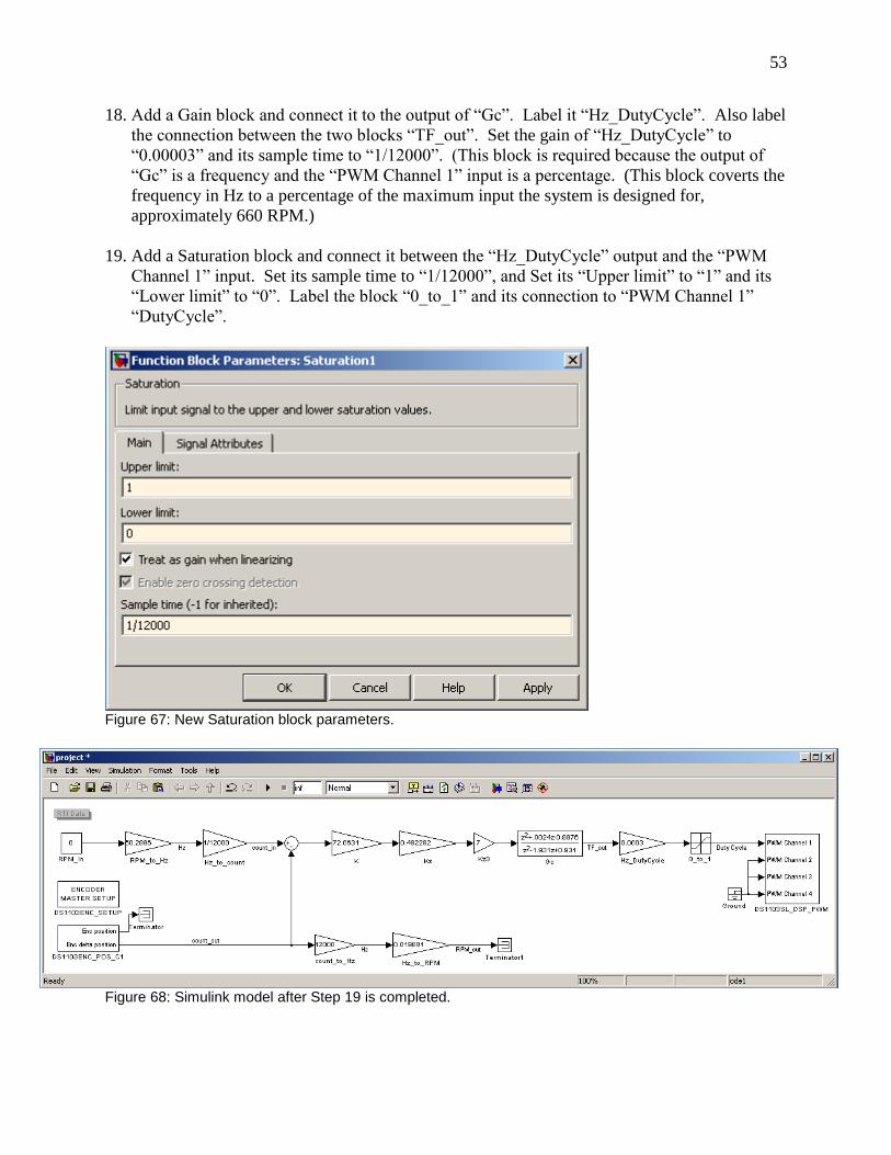
18. Add a Gain block and connect it to the output of “Gc”. Label it “Hz_DutyCycle”. Also label

the connection between the two blocks “TF_out”. Set the gain of “Hz_DutyCycle” to

“0.00003” and its sample time to “1/12000”. (This block is required because the output of

“Gc” is a frequency and the “PWM Channel 1” input is a percentage. (This block coverts the

frequency in Hz to a percentage of the maximum input the system is designed for,

approximately 660 RPM.)

19. Add a Saturation block and connect it between the “Hz_DutyCycle” output and the “PWM

Channel 1” input. Set its sample time to “1/12000”, and Set its “Upper limit” to “1” and its

“Lower limit” to “0”. Label the block “0_to_1” and its connection to “PWM Channel 1”

“DutyCycle”.

Figure 67: New Saturation block parameters.


54

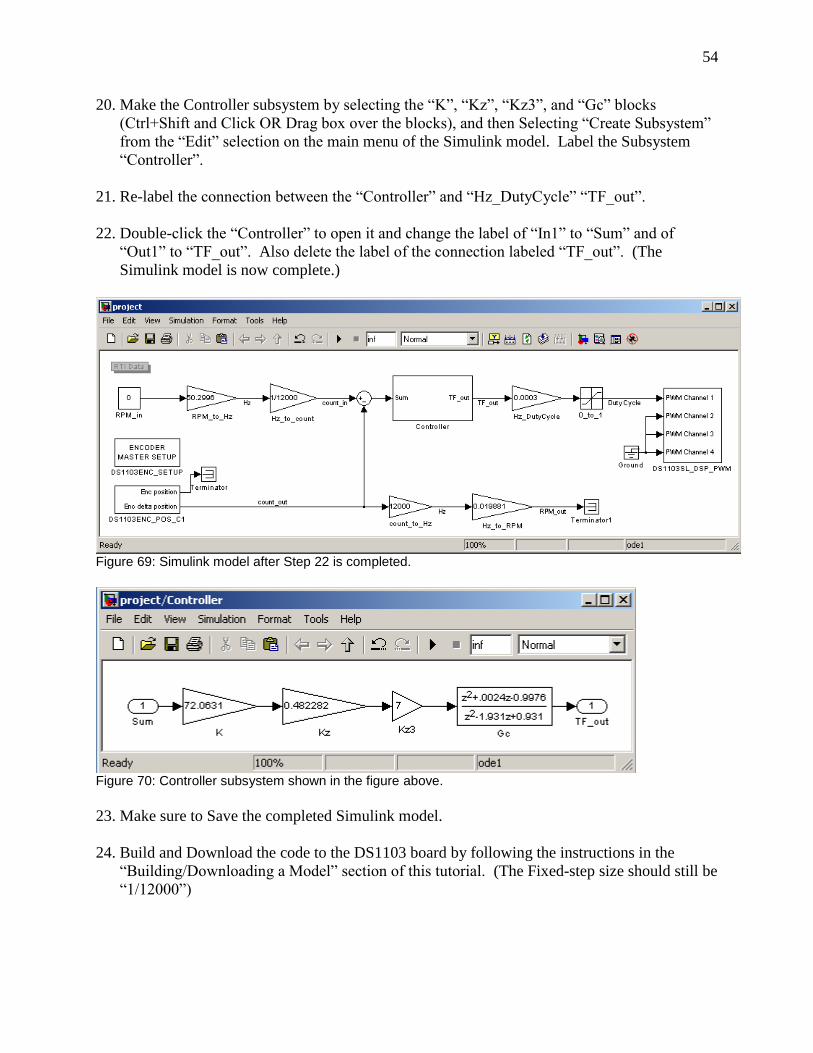
20. Make the Controller subsystem by selecting the “K”, “Kz”, “Kz3”, and “Gc” blocks

(Ctrl+Shift and Click OR Drag box over the blocks), and then Selecting “Create Subsystem”

from the “Edit” selection on the main menu of the Simulink model. Label the Subsystem

“Controller”.

21. Re-label the connection between the “Controller” and “Hz_DutyCycle” “TF_out”.

22. Double-click the “Controller” to open it and change the label of “In1” to “Sum” and of

“Out1” to “TF_out”. Also delete the label of the connection labeled “TF_out”. (The

Simulink model is now complete.)


Figure 70: Controller subsystem shown in the figure above.

23. Make sure to Save the completed Simulink model.

24. Build and Download the code to the DS1103 board by following the instructions in the

“Building/Downloading a Model” section of this tutorial. (The Fixed-step size should still be

“1/12000”)

55

25. Now, it is time to edit the ControlDesk layout. Open the existing layout and follow the

instructions in the “Monitoring/Controlling/Recording Values” section of this tutorial to

Connect the following variables/values to the type of instrument(s) indicated.

a. RPM_in: Display, Slider, NumericInput, and PlotterArray. (Change the Max Range

of the Slider and NumericInput to “660”.)

b. RPM_out: Display and PlotterArray

c. DutyCycle: Display

Figure 71: Layout in ControlDesk with system running and slider used to change RPM_in.

56

26. Observe that using the NumericInput for RPM_in provides for better observation of the

actual Step Response of the System. Also observe that if voltage is applied to the brake,

especially at mid-range input values, the DutyCycle will increase to compensate and

maintain RPM_out near the desired value. (Generally RPM_in of 200 RPM was used in

testing. For high speed inputs such as 660 RPM, RPM_out will show decreases in its value

as more brake voltage is applied but will e stable.)

Note: The maximum value before the brake stops is around 10+ Volts if the voltage is

increased slowly. Dropping the voltage to somewhere between 5 and 8 Volts should cause

the motor to start running again, but it may take some time for the system to start the motor

and stabilize its speed.

27. In order to record data, Add a CaptureSettings instrument by following the instructions in the

“CaptureSettings Instrument” subsection of the “Monitoring/Controlling/Recording Values”

section of this tutorial.

Figure 72: ControlDesk layout with CaptureSettings instrument added and the system running. (Step response for 200 RPM observed using NumericInput to change RPM_in from 0 to 200 while system was running.)

28. Capture data and Plot it in MATLAB. (This is also explained in the “CaptureSettings

Instrument” subsection mentioned in Step 27 above.)

57

29. Now, for another cool feature of ControlDesk. The value of any gain or constant block in the

Simulink model can be changed without rebuilding and downloading code and while the

system is running. (There might be other blocks that work as well.) Use the instructions in

the “Monitoring/Controlling/Recording Values” section of this tutorial to connect “Kz3”

(Gain) to a Display and a NumericInput instrument in the ControlDesk Layout.

30. Apply 10 Volts to the brake. Set RPM_in to “0”. Start the CaptureSettings instrument.

Quickly change RPM_in to “200”. Observe RPM_out on its PlotterArray, and quickly Stop

the CaptureSettings instrument before the 0 to 200 transition disappears. The data can be

plotted in MATLAB if desired.

31. Set “Kz3” to “20” and repeat Step 30 above. Compare the results. (There should be a visible

spike/overshoot in RPM_out for Kz3 = 20 that is not in the Kz3 = 7 RPM_out output.)

Figure 73: ControlDesk layout with Kz3 instruments added and system running with RPM_out response to RPM_in=200, Kz3=20, and brake voltage=10V shown.

32. Set the brake voltage to 0 Volts and “Kz3” back to “7” The tutorial is completed.

58

References

[1] “DS1103 PPC Controller Board”, Germany: dSPACE, July 2008.

[2] Annemarie Thomas. "dSPACE DS1103 Control Workstation Tutorial and DC Motor Speed

Control: Project Report", Senior Project Report, Bradley University ECE Department, May

2009.

[3] “Connector and LED Panels,” Catalog 2008, Germany: dSPACE GmbH, 2008, p. 302.

[4] ControlDesk Experiment Guide For ControlDesk 3.2, Germany: dSPACE GmbH, 2008,

Release 6.1.

[5] dSPACE System First Work Steps For DS1103, DS1104, DS1005, DS1006, and Micro Auto

Box, Germany: dSPACE GmbH, 2007, Release 6.0.

[6] Real-Time Interface (RTI and RTI-MP) Implementation Guide, Germany: dSPACE GmbH,

2008, Release 6.1.

[7] DS1103 PPC Controller Board Hardware Installation and Configuration, Germany:

dSPACE GmbH, 2007, Release 6.0.

Documents

dSPACE DS1103 Control Workstation Tutorial and DC Motor ...ee.bradley.edu/projects/proj2009/dscntrl/Tutorial.pdf · dSPACE DS1103 Control Workstation Tutorial and DC ... to become