DSP LAB REPORT

March 31, 2009

Submitted by

1. Arunkumar B060403EC

2. Febin George B060190EC

3. Sabu Paul B060310EC

4. Sareena T.A B060125EC

1

Complex Plane

All complex numbers can be represented on the complex plane. Complex num-bers are represented either as x+iy or in the angle magnitude form. As is obvi-ous, the x-axis is used to represent the real part of the number and the complexpart is represented on the y-axis. As part of our Matlab familiarization exercisewe tried plotting a circle on the complex plane.

Plotting a circle on the complex plane

For plotting a circle we have to generate a set of complex numbers which lie onthe circle. A circle is always easiest to represent in the angle magnitude form.Therefore, the set of complex numbers is

z = reiθ; θ =2kπN

; k∀0, 1, ...2π(N − 1)N

r = 1⇒ unit circle

The Matlab plotting function accepts cartesian coordinate values. Thereforewe convert the angle magnitude representation to cartesian system.

abcissa = cos(2kπN

)

ordinate = sin(2kπN

)

The plot of the unit circle in the complex plane is as follows

2

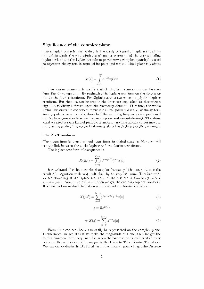
Signicance of the complex plane

The complex plane is used widely in the study of signals. Laplace transformis used to study the characteristics of analog systems and the correspondings-plane where s is the laplace transform parameter(a complex quantity) is usedto represent the system in terms of its poles and zeroes. The laplace transformis

F (s) =

∞∫−∞

e−stx(t)dt (1)

The fourier transorm is a subset of the laplace transorm as can be seenfrom the above equation. By evaluating the laplace tranform on the jωaxis weobtain the fourier tranform. For digital systems too we can apply the laplacetranform. But then, as can be seen in the later sections, when we discretize asignal, periodicity is forced upon the frequency domain. Therefore, the wholes-plane becomes unnecessary to represent all the poles and zeroes of the system.As any pole or zero occuring above half the sampling frequency disappears andin it's place generates false low frequency poles and zeroes(aliasing). Therefore,what we need is some kind of periodic transform. A circle quickly comes into ourmind as the angle of the vector that moves along the circle is a cyclic parameter.

The Z - Transform

The z-transform is a custom made transform for digital systems. Here, we willsee the link between the z, the laplace and the fourier transforms.

The laplace tranform of a sequence is

X(jω′) =N−1∑n=0

(eσ+jωTs)−nx[n] (2)

here ω′stands for the normalised angular frequency. The summation is theresult of integration with x(t) multiplied by an impulse train. Therfore whatwe see above is just the laplace transform of the discrete version of x(t) wheres = σ+ jωTs. Now, if we put ω = 0 then we get the ordinary laplace tranform.If we instead make the attenuation σ zero we get the fourier transform.

X(jω′) =N−1∑n=0

(RejωTs)−nx[n] (3)

z = RejωTs (4)

⇒ X(z) =N−1∑n−0

z−nx[n] (5)

From 4 we can see that z can easily be represented on the complex plane.Furthermore, we see that if we make the magnitude of z one, then we get thefourier tranform of the sequence. So, when the z-transform is evaluated at everypoint on the unit circle, what we get is the Discrete Time Fourier Transform.We can also evaluate the DTFT at just a few discrete points to get the Discrete

3

Fourier Transform. If we take too few points then there is the possibility oftime domain aliasing. Thus, we nish with the write-up on the z-transform andproceed to demonstrate a simple application.

A simple lter

We can just create an arbitrary sequence and evaluate its DFT using the z-transform and our t algorithm. Then we will compare them to see if they arethe same.

h[n] = [1, 2, 4, 5]

H(z) = 1 + 2z−1 + 4z−2 + 5z−3

Here, we evaluate the z- transform at 64 points around the unit circle. Thefollowing is the z-transforms absolute value.

4

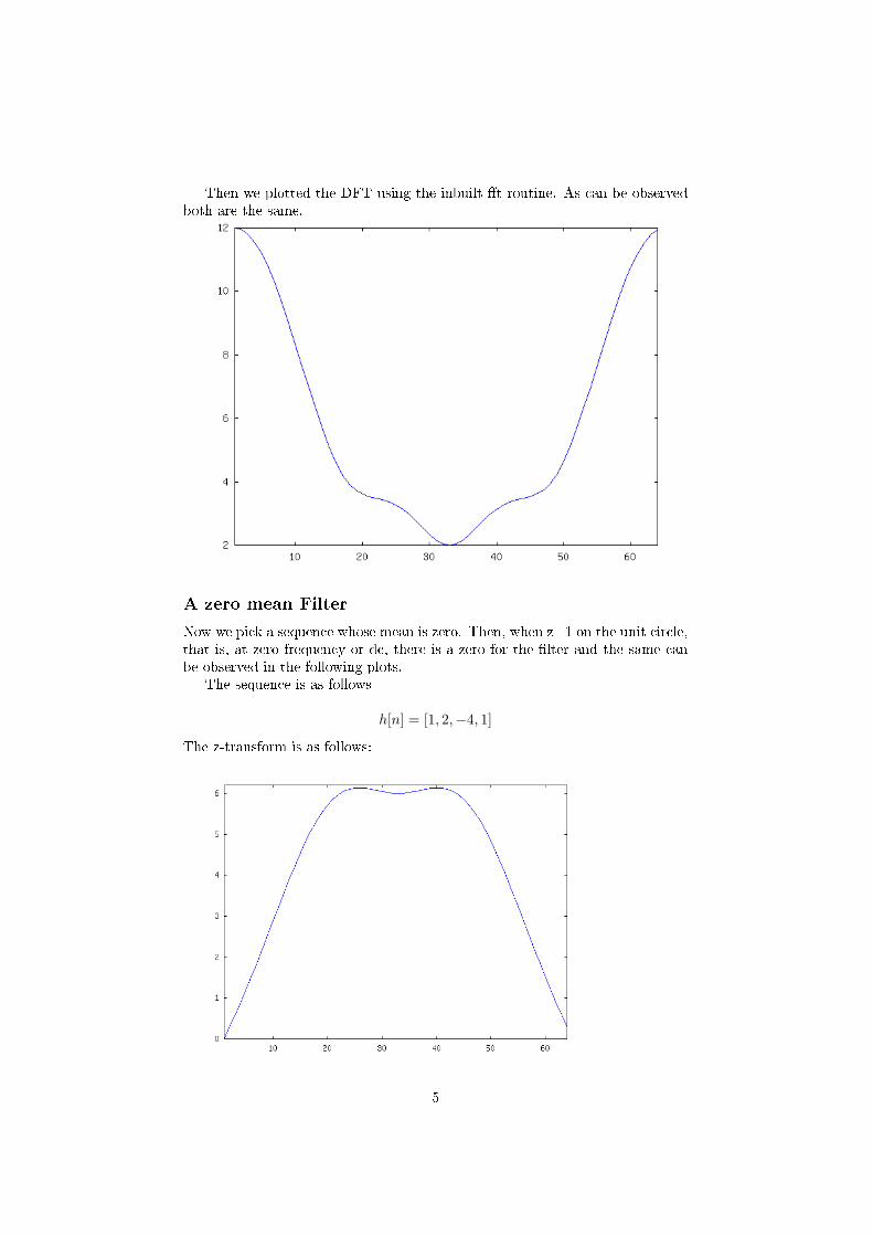
Then we plotted the DFT using the inbuilt t routine. As can be observedboth are the same.

A zero mean Filter

Now we pick a sequence whose mean is zero. Then, when z=1 on the unit circle,that is, at zero frequency or dc, there is a zero for the lter and the same canbe observed in the following plots.

The sequence is as follows

h[n] = [1, 2,−4, 1]

The z-transform is as follows:

5

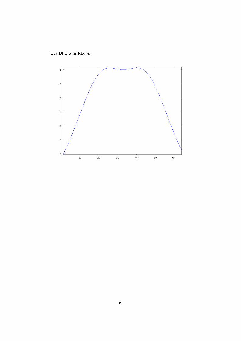
The DFT is as follows:

6

The code for plotting the z-transform for an ordinary sequence is as follows

%sequence

h = [1,2,3,4];

%number of points on the unit circle

N = 64;

%determine the points

z = complex(cos(2*pi/N*(0:N-1)),sin(2*pi/N*(0:N-1)));

%evaluate H(z) at each point

for i = 1:N

H(i) = 1+2*z(i)^-1+3*z(i)^-2+4*z(i)^-3;

end

%plot the unit circle

plot(z)

%plot the value of H(z) along the unit circle

figure

plot(abs(H))

%plot the N-point DFT of h(n)

figure

plot(abs(fft(h,64)))

The code for plotting the z-transform for a zero mean sequence is as shownbelow

%zero mean sequence

h = [1,-2,-1,2];

%number of points on the unit circle

N = 64;

%determine the chosen points

z = complex(cos(2*pi/N*(0:N-1)),sin(2*pi/N*(0:N-1)));

%evaluate H(z) at each point

for i = 1:N

H(i) = 1-2*z(i)^-1-1*z(i)^-2+2*z(i)^-3;

end

%plot the unit circle

plot(z)

%plot the value of H(z) along the unit circle

figure

plot(abs(H))

7

%plot the N-point DFT of h(n)

figure

plot(abs(fft(h,64)))

The Fast Fourier Transform

A summary of the results used.

Fourier Transform

The fourier transform is one of the most widely used mathematical tools in thestudy of signals. The fourier transform of an analog causal signal is given bythe relation -

X(jω) =∫ α

0

x(t)e−jωtdt (6)

How it is obtained...

The continuous fourier transform is obtained from the fourier series thatis used for periodic signals. In fourier series the smallest discrete frequency isgiven by

D = 1/L (7)

The strength of each frequency is the dot product of that frequency compo-nent and the signal in any one complete period.

As we let L tend to innity the smallest frequency starts tending to zero andthe evaluation of the strength of a particular frequency reduces to evaluating anintegral. Digging deeper, fourier sequence is arrived at by using the principle oforthogonal signals.

Discretization in Time Domain

Analysis of signals in the continuous time domain is useful for the design ofanalog signal manipulation devices like analog lters, various control systemsetc.. Bu nowadays all signals are processed and transmitted digitally. There area lot of things that are made easier with this approach, some of which include-low noise, easy manipulation and compatibility with existing computer systems.

How Is discretization in the time domain carried out?

The time domain signal is multiplied by an impulse train to eect sampling inthe time domain. Then we round the sampled values to the nearest discretelevel. For now we don't consider the eect of the latter stage. The multiplyingof the signal by an inpluse train is just a nice way of looking at the process.Practically, it is carried out by a sample and hold circuit in conjunction withan ADC.

xsampled(t) =∞∑

i=−∞δ(t− i ∗ Ts) ∗ x(t) (8)

8

⇒

xsampled(t) =∞∑i=0

x(i ∗ Ts) ∗ δ(t− i ∗ Ts) (9)

Now,

δ(jω) =2πTs

∞∑−∞

δ(ω − i ∗ 2 ∗ πTs

) (10)

The discrete time fourier transform of the signal is the continuous timefourier transform of 9.

X(jω) =∞∑i=0

x(i ∗ Ts) ∗ e−jω∗i∗Ts (11)

This is given by the convolution of the FT of x(t) with that of the impulsetrain, which results in a periodic FT with the original FT repeating with thesame frequency as that of the impulse train's transform. Nyquist's samplingtheorem is based on this fact. The minimum gap between two impulses in thefrequency domain should be 2*F to prevent aliasing.

FT of the sampled signal is

2πTsX(jω) ∗ ∗

∞∑i=−∞

δ(ω − i ∗ 2 ∗ πTs

) (12)

⇒ Xsampled(jω) =2πTs∗∞∑

i=−∞X(ω − i ∗ 2

π

Ts) (13)

As long as the Nyquist criterion is satised the frequency domain represen-tation is unique and the original signal can be got back by using a low passlter.

Eecting Sampling in the frequency domain

The sampling process can now be repeated on the continuous frequency domainin such a manner that there is no time domain aliasing. Therefore the mini-mum sampling interval in the frequency domain is 1

N . Now both frquency andtime domains have been sampled. Now the transform is called Discrete FourierTransform as it deals with discrete times and frequencies. Therfore the DFT ofthe sampled time domain signal is

X(k) =N−1∑i=0

x(nTs) ∗ e−j2πN knTs (14)

The shorthand notation is

X(k) =N−1∑i=0

x(nTs) ∗W knN (15)

9

Fast algorithms for evaluating DFT

The evaluation of the DFT from its formula is slow and impractical in many caseswhere millions of samples are involved. Here is where the Fast Fourier Transformcomes in. It uses the periodic properties of the transforming function to evaluatethe DFT using a fewer number of operations. There are many algorithms whichhave dierent pros and cons. In the lab we have implemented the Decimation inTime FFT algorithm with radix 2. Therefore all the input sequences will haveto be powers of 2 in length.

The mathematical formulation of the DIT algorithm is based on the followingresult.

x(n) can be split into even and odd indexed samples.

The even indexed samples are x(2m) and the odd indexed samples arex(2m+1) where m varies from 0 to N/2 -1.

Therefore,

X(k) =N/2−1∑m=0

x(2m)W k∗2mN +

N/2−1∑m=0

x(2m+ 1)W k∗(2m+1)N (16)

Let, g(m) = x(2m) and h(m) = x(2m+ 1)

⇒ X(k) =N/2−1∑m=0

g(m)W kmN/2 + (

N/2−1∑m=0

h(m)W kmN/2) ∗W k

N (17)

⇒ X(k) = G(k) +W kNh(k) (18)

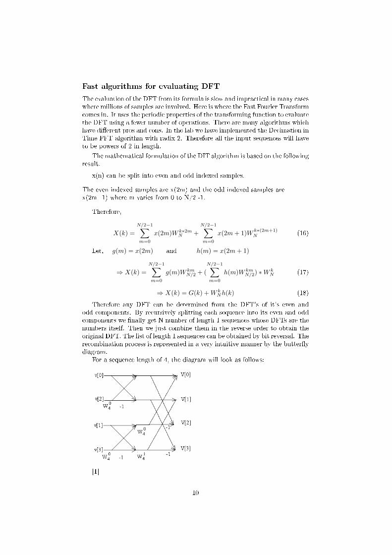
Therefore any DFT can be determined from the DFT's of it's even andodd components. By recursively splitting each sequence into its even and oddcomponents we nally get N number of length 1 sequences whose DFTs are thenumbers itself. Then we just combine them in the reverse order to obtain theoriginal DFT. The list of length 1 sequences can be obtained by bit reversal. Therecombination process is represented in a very intuitive manner by the butterydiagram.

For a sequence length of 4, the diagram will look as follows:

[1]

10

Experimenting with FFTCreating an arbitrary sequence and determining its FFT

octave-3.0.1:11> x=1:128

octave-3.0.1:12> y=myfft(x,128);

octave-3.0.1:13> index=0:1/128:127/128;

octave-3.0.1:14> plot(index,abs(y))

octave-3.0.1:15> print("figure.png")

octave-3.0.1:16> replot

The y-axis values should be scaled according to the sampling frequency.The FFT of a sine waveoctave-3.0.1:23> x=1:128;

octave-3.0.1:24> y=sin(x);

octave-3.0.1:25> z=myfft(y,128);

octave-3.0.1:26> plot(index,abs(z))

11

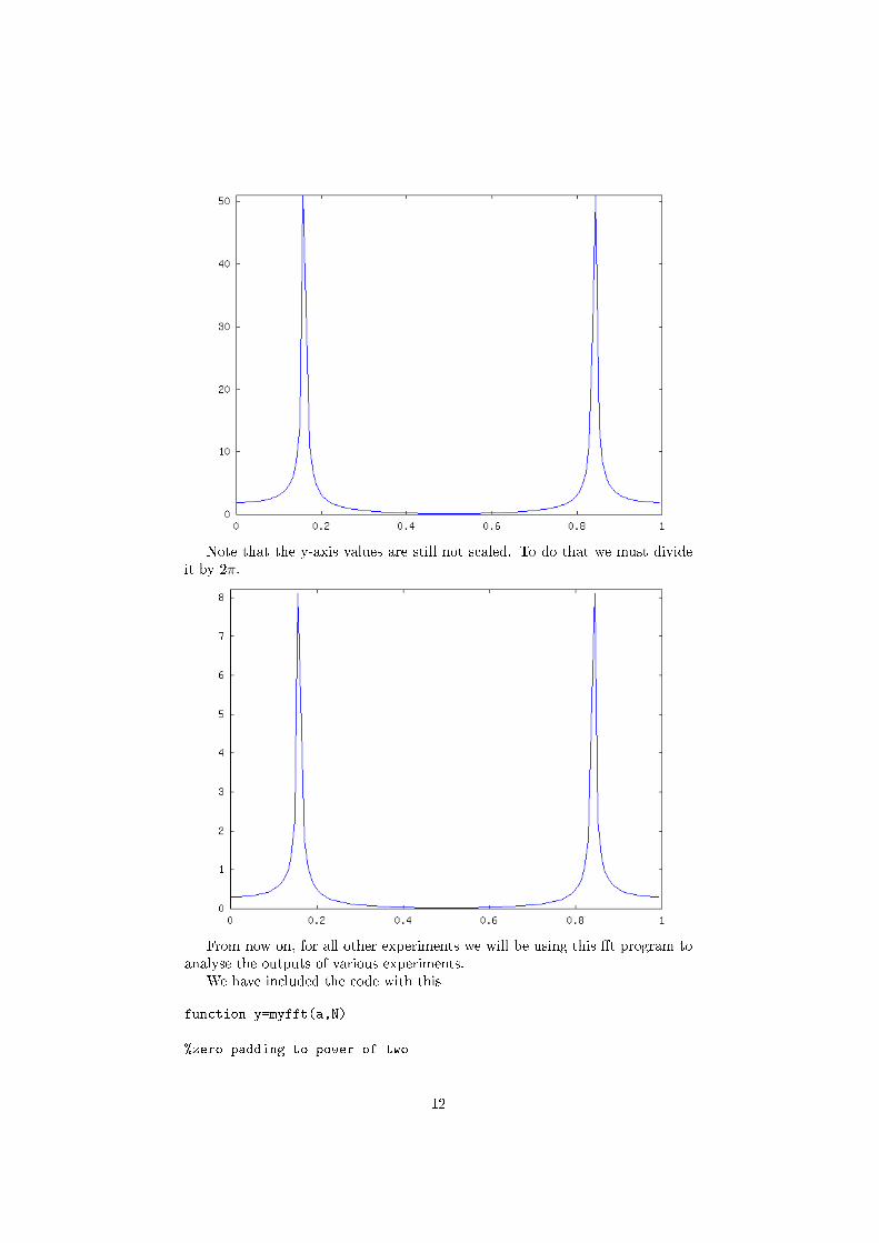
Note that the y-axis values are still not scaled. To do that we must divideit by 2π.

From now on, for all other experiments we will be using this t program toanalyse the outputs of various experiments.

We have included the code with this

function y=myfft(a,N)

%zero padding to power of two

12

i = N;

temp = 0;

while (i>0)

i = floor(i/2);

temp = temp+1;

end

n = temp;

if (N ~= 2^(n-1))

a(length(a)+1:2^n) = 0;

N_ = 2^n;

n_ = n;

else

a(length(a)+1:2^(n-1)) = 0;

N_ = 2^(n-1);

n_ = n-1;

end

%bit reversal

for k = 1:n_

for l = 1:2^(k-1)

j = 1;

for i = 1:2:N_/2^(k-1)-1

b(j+(l-1)*N_/2^(k-1)) = a(i+(l-1)*N_/2^(k-1));

b(j+N_/2^k+(l-1)*N_/2^(k-1)) = a(i+1+(l-1)*N_/2^(k-1));

j = j+1;

end

end

a = b;

end

a_ = b;

%butterfly stages

w = exp(complex(0,-2*pi/N_));

for i = 1:n_

for j = 1:2^(n_-i)

for k = 1+(2^i)*(j-1):(2^i)*(j-1)+2^(i-1)

temp = w^(2^(n_-i)*(k-1));

temp1 = temp*a_(k+2^(i-1));

temp2 = a_(k) - temp1;

a_(k) = a_(k) + temp1;

a_(k+2^(i-1)) = temp2;

end

end

end

y = a_;

return

13

Convolution

This is the process by which the output of a system whose impulse responseis known, is determined for a paticular input. Convolution of two sequencesis equilvalent to taking the product of their DFTs. The idea of convolution issimple enough. For each input sample one whole impulse response, scaled bythe input sample is produced at the output. The outputs corresponding to allthe input samples are added to give the nal output. From this explanation wecan quickly write down a formula for it.

y[n] =∞∑k=0

x[k] ∗ h[n− k] (19)

But, there are sometimes situations where the entire input sequence is verylarge and we need to do the convolution on smaller chunks of the input. Thereare two methods that we tried in the lab for this.

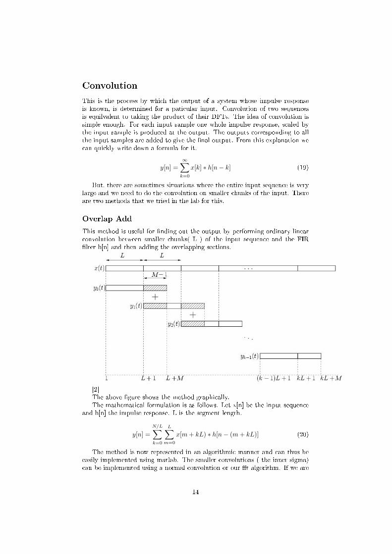
Overlap Add

This method is useful for nding out the output by performing ordinary linearconvolution between smaller chunks( L ) of the input sequence and the FIRlter h[n] and then adding the overlapping sections.

[2]The above gure shows the method graphically.The mathematical formulation is as follows. Let x[n] be the input sequence

and h[n] the impulse response. L is the segment length.

y[n] =N/L∑k=0

L∑m=0

x[m+ kL) ∗ h[n− (m+ kL)] (20)

The method is now represented in an algorithmic manner and can thus beeasily implemented using matlab. The smaller convolutions ( the inner sigma)can be implemented using a normal convolution or our t algorithm. If we are

14

using the t algorithm then we must take care to pad the sequences with enoughnumber of zeroes to prevent aliasing. The code has been included to make thealgorithm clear.

function y=febovadd(a,b)

m = length(a);

n = length(b);

s = rem(m,20);

p = floor(m/20);

if s==0

k=p;

else

k=p+1;

a(m+1:20*k)=0;

end

l(1:20*k +n -1)=0;

g=l;

for i =1:k;

c = a(20*(i-1) +1:20*i);

f = febconv(c,b);

length(f);

l(20*(i-1)+1:20*(i-1)+19+n)=f(1:19+n);

g =g+l;

l(1:44)=0;

endfor

y=g(1:m+n-1);

return

15

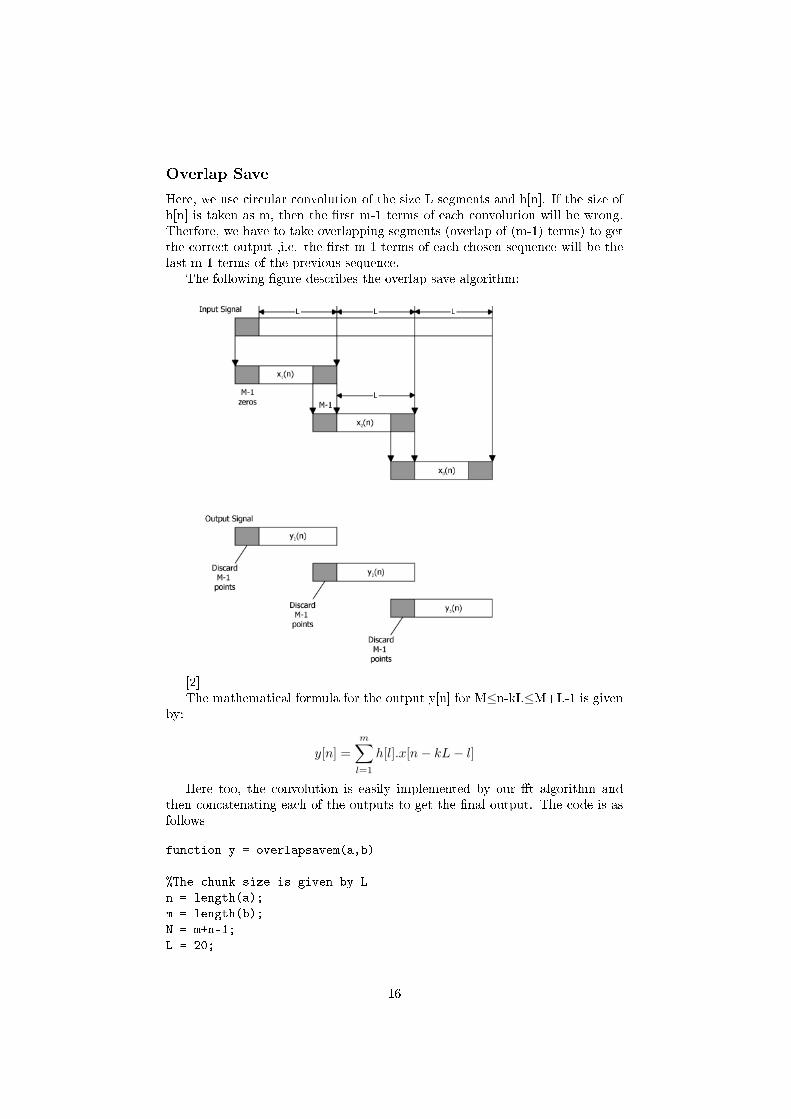
Overlap Save

Here, we use circular convolution of the size L segments and h[n]. If the size ofh[n] is taken as m, then the rst m-1 terms of each convolution will be wrong.Therfore, we have to take overlapping segments (overlap of (m-1) terms) to getthe correct output ,i.e. the rst m-1 terms of each chosen sequence will be thelast m-1 terms of the previous sequence.

The following gure describes the overlap save algorithm:

[2]The mathematical formula for the output y[n] for M≤n-kL≤M+L-1 is given

by:

y[n] =m∑l=1

h[l].x[n− kL− l]

Here too, the convolution is easily implemented by our t algorithm andthen concatenating each of the outputs to get the nal output. The code is asfollows

function y = overlapsavem(a,b)

%The chunk size is given by L

n = length(a);

m = length(b);

N = m+n-1;

L = 20;

16

%Zero padding

a_(1:m-1) = 0;

a_(m:N) = a(1:n);

remainder=rem(N-L,L-(m-1));

remainder=L-(m-1)-remainder;

a_(N+1:N+remainder) = 0;

b(m+1:L) = 0;

n=ceil((N-L)/(L-m-1));

n=n+1;

x=[];

%overlap save

for i = 1:n

temp = circconv(a_(1+(i-1)*(L-m+1):L+(i-1)*(L-m+1)),b);

x = cat(2,x,temp(m:L));

end

y = x(1:N);

return

FIR Filters

FIR or nite impulse response lters are called so because their impulse settlesto zero in a nite number of sample intervals. Since the transfer function lackspoles their output depends only on the present and past values of the input andnot at all on the output, or in other words they lack internal feedback.

The frequency response of an ideal lowpass lter with a cuto frequency ωcis given by

H(s) =

1 for |ω|≤ωc0 otherwise

The corresponding impulse response will be

h(n) = 2fcsinc(2fcn) −∞ < n <∞

where fc=ωc2Π

Thus we observe that the impulse response of an ideal lowpass lter is bothinnite and non-causal. We can make it causal by taking a nite range for ncentered at n=0 (i.e. −N2 to N

2 ) and then shifting it to the right by N2 .

What we are doing here is equivalent to multiplying the impulse responseby a rectangular window of size N and then shifting it.

Gibbs Phenomenon:

The frequency response of such a lter will have many ripples in the transitionregion.

17

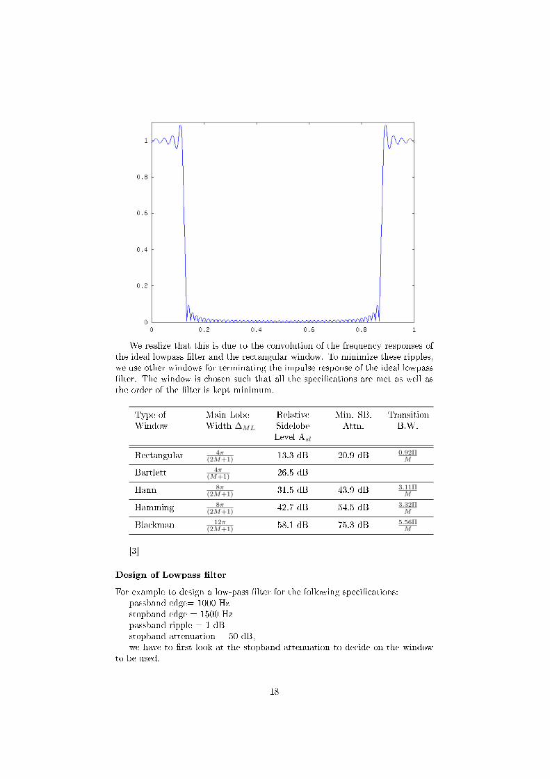
We realize that this is due to the convolution of the frequency responses ofthe ideal lowpass lter and the rectangular window. To minimize these ripples,we use other windows for terminating the impulse response of the ideal lowpasslter. The window is chosen such that all the specications are met as well asthe order of the lter is kept minimum.

Type ofWindow

Main LobeWidth ∆ML

RelativeSidelobeLevel Asl

Min. SB.Attn.

TransitionB.W.

Rectangular 4π(2M+1) 13.3 dB 20.9 dB 0.92Π

M

Bartlett 4π(M+1) 26.5 dB

Hann 8π(2M+1) 31.5 dB 43.9 dB 3.11Π

M

Hamming 8π(2M+1) 42.7 dB 54.5 dB 3.32Π

M

Blackman 12π(2M+1) 58.1 dB 75.3 dB 5.56Π

M

[3]

Design of Lowpass lter

For example to design a low-pass lter for the following specications:passband edge= 1000 Hzstopband edge = 1500 Hzpassband ripple = 1 dBstopband attenuation = 50 dB,we have to rst look at the stopband attenuation to decide on the window

to be used.

18

From the table shown above we observe that the Hamming window oerssuch a stopband attenuation of 53 dB.

The order of the lter N is given by

N =4.fs

transitionwidth

In this case, we obtain N as 66.The h(n) which is shifted by N

2 is now given by

h′(n) = 2fcsinc(2fc(n− 33))

And the Hamming window

w(n) = 0.58386− 0.41614cos(2ΠnN − 1

) 0 ≤ n ≤ N

Therefore, the windowed response is

hlp(n) = h′(n).w(n) 0 ≤ n ≤ N

It has a DFT as shown below

It can be observed that the lter multiplied with the Hamming window givesa much better ripple performance than the one multiplied with the rectangularwindow.

19

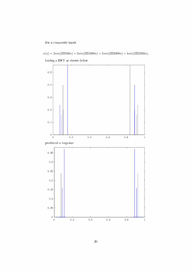
For a composite input

x(n) = 2sin(2Π500n) + 3sin(2Π1000n) + 5sin(2Π2000n) + 4sin(2Π2500n),

having a DFT as shown below

produced a response

20

Design of Bandpass lter

In the previous section we designed a lowpass lter. We can then use a similarapproach with a slight modication to design a bandpass lter. To transforman ideal lowpass lter into a bandpass lter, we need to shift the rectangularwindow in the frequency domain, such that it is no longer centred at zero, butat the mean of our required pass band (fm). This can be done by convolving thefrequency response with an impulse located at that frequency, which is eectivelymultiplying the impulse response with a cosine function having a frequency offm.

Consider the design of a bandpass lter whose passband ranges from ω1toω2.

=⇒ ωm =ω1 + ω2

2The impulse response of an ideal lowpass lter is

h(n) = 2fcsinc(2fcn) −∞ < n <∞

here,

fc = f2 − fm = fm − f1

Now, let us shift it such that the frequency response is now centred aboutfm

h′(n) = h(n).cos(ωmn)

=⇒ h′(n) = 2fcsinc(2fCn)cos(ωmn)

Once h'(n) is obtained, we can proceed in a similar fashion as the lowpass l-ter design. i.e. h'(n) is then terminated by multiplying it with an appropriatelychosen window to obtain the bandpass impulse response hbp(n).

hbp(n) = h′(n).w(n)

For a given specication a bandpass lter with the following frequency spec-trum was designed

21

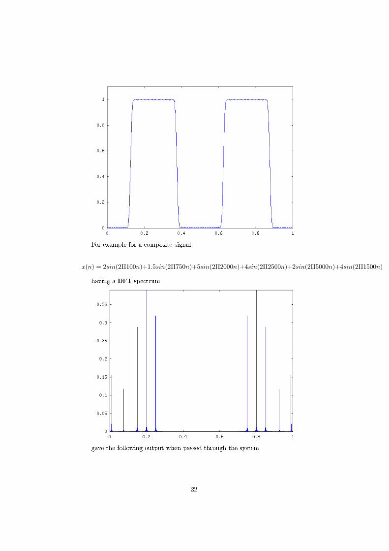
For example for a composite signal

x(n) = 2sin(2Π100n)+1.5sin(2Π750n)+5sin(2Π2000n)+4sin(2Π2500n)+2sin(2Π5000n)+4sin(2Π1500n)

having a DFT spectrum

gave the following output when passed through the system

22

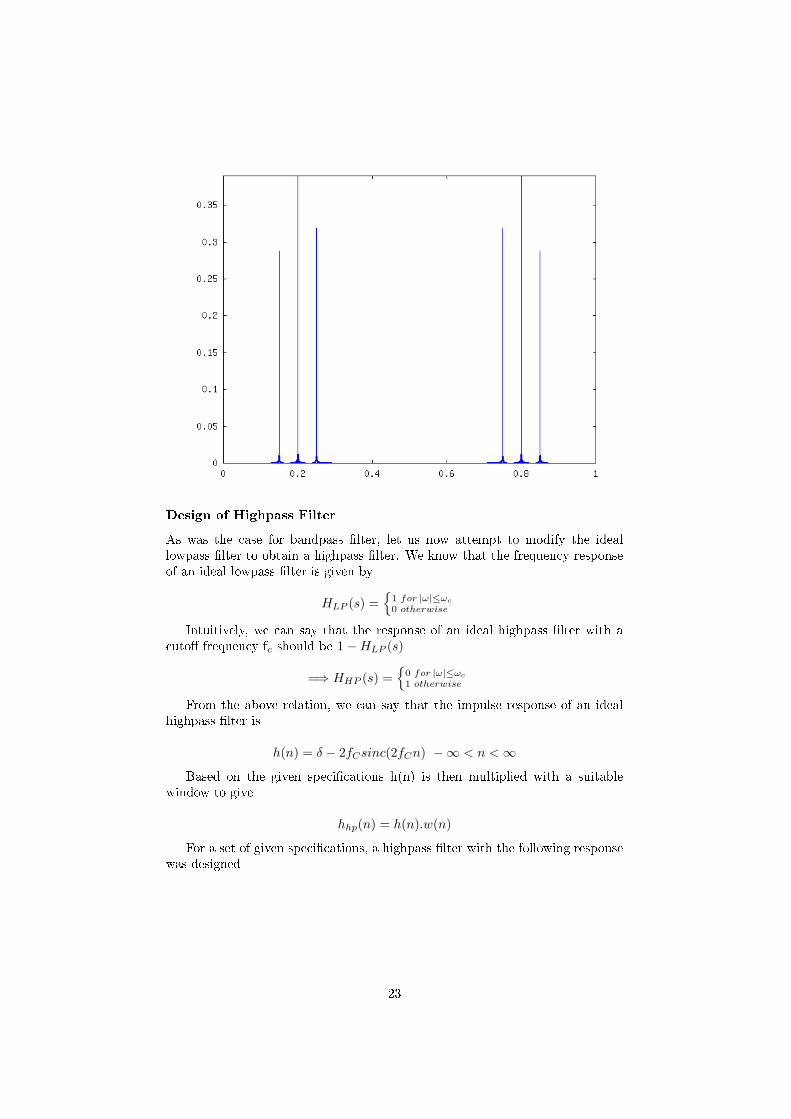
Design of Highpass Filter

As was the case for bandpass lter, let us now attempt to modify the ideallowpass lter to obtain a highpass lter. We know that the frequency responseof an ideal lowpass lter is given by

HLP (s) =

1 for |ω|≤ωc0 otherwise

Intuitively, we can say that the response of an ideal highpass lter with acuto frequency fc should be 1−HLP (s)

=⇒ HHP (s) =

0 for |ω|≤ωc1 otherwise

From the above relation, we can say that the impulse response of an idealhighpass lter is

h(n) = δ − 2fCsinc(2fCn) −∞ < n <∞

Based on the given specications h(n) is then multiplied with a suitablewindow to give

hhp(n) = h(n).w(n)

For a set of given specications, a highpass lter with the following responsewas designed

23

For a composite input

x(n) = 2sin(2Π500n) + 3sin(2Π1000n) + 5sin(2Π2000n) + 4sin(2Π2500n)

having a DFT spectrum

the following output was obtained

24

IIR Filters

Innite Impulse Response Filters are called so because their impulse responsedoes not settle to zero in a nite number of sample intervals, or in other wordsthey have internal feedback.

Discrete-time IIR lters can be designed from continuous-time lters byusing either of two approaches:

• Impulse invariance.

• Bilinear transformation.

So, rst we have to design a continuous time lter that matches our specica-tions. Then we use one of these methods to make the correspoding digital lter.This method is chosen because analog approximation techniques are very welldeveloped.

The process of designing a continuous time lter is basically just aboutplacing a certain number of poles in the complex plane. There are are dierentsystems that are followed which yield dierent magnitude responses. Examplesare butterworth, chebychev, elliptic etc.

We have designed lters using the butterworth and chebychev approxima-tions.

Designing continuous time lters

Butterworth Approximation

In the Butterworth lter the poles are placed on the circumference of acircle having a radius equal to the continuous-time cut-o frequency (Ωc). Themathematical formula for the magnitude of the tranfer function is given by

25

|H(ω)| = 1√1 + ( Ω

Ωc)2N

where N is the order of the lter.Once Ωc and 2N are obtained by substituting the given specications in the

above formula, a circle of radius Ωcis drawn and N equidistant poles are markedon its circumference such that each pole is given by

pn = ωcej( Π

2 −Π

2N +n ΠN )

Only the poles in the Left Hand Plane is taken to design the lter. Once thepoles are obtained, the tranfer function will be given as

H(s) =ωNc

(s− p1)(s− p2)...(s− pN )

As an example, an order 4 lter with cut-o frequency ω0 is shown here.

[2]

Chebychev Approximation

The poles in the Chebychev lter are placed on the circumference of an ellipsewhose major axis is 2ωmajand minor axis 2ωmin. The mathematical formula forthe magnitude of the tranfer function is given by

H(ω) =1√

1 + ε2.T 2( ωωp )

wherefor |x|≤1

T (x) = cos(Ncos−1(x))

for |x|>1

T (x) = cosh(Ncosh−1(x))

The specications are substituted in the above formula, and thereby εand Nare obtained.

26

The quantity αis obtained as

α = ε−1 +√

1 + ε−2

Once αis obtained ωmajand ωminare obtained by

ωmaj =12

(α1N + α

−1N ).ωp

ωmin =12

(α1N − α

−1N ).ωp

The ellipse is then drawn and the poles are marked on its circumference suchthat

pn = ωmincos(φn) + jωmajsin(φn)

where φnis given by

φn =Π2− Π

2N+ n

ΠN

As in Butterworth, only the poles in the Left Half Plane are used to formthe transfer function, from which the z-transform is similarly obtained and thesecond order parallel form implemented.

Once the continuous time lter has been designed then, we need to convertit to the digital domain. We will use the two methods mentioned earlier

Converting analog design to digital domain

Impulse Invariance

In the impulse invariance method the impulse response of the continuous-time system is sampled to produce the impulse response of the discrete-timesystem. For a band-limited continuous-time system the frequency response ofthe discrete-time system will be same as the continuous-time system's frequencyresponse with linearly-scaled frequency. i.e. if the continuous-time system hasan impulse response hc(t) and it is sampled at time period T, the impulseresponse of the discrete-time system h(n) will be given by

h(n) = T.hc(nT )

And their frequency responses have a relation given by

H(ejω) =∞∑

k=−∞

Hc(jω

T+ j

2ΠTk)

And if the continuous-time response is band-limited, the frequency response (for|ω|<Π) is

H(ejω) = Hc(jω

T)

In impulse invariance method, the relation between continuous-time and discrete-time frequencies is linear, i.e.

27

Ω =ω

T

Once the specications for the lter, i.e. the discrete-time frequencies and thestop-band and pass-band attenuations are given, the corresponding continuous-time frequencies are obtained using the above relation. Then we decide whetherwe want to use a butterworth or a chebychev approximation. Once that isdecided we use the corresponding magnitude response formulae and the givenspecications to calculate the order of the lter.

After we determine the order of the lter, we nd out the pole locations usingthe corresponding formula. Thus, we obtain the transfer function of the system.Then we split it into its partial fractions. We convert each term, then, to thez domain. Because, there are complex poles, we don't as yet have a practicallyrealizabe lter. Thus, we combine the conjugate poles to obtain second orderterms. We then implement each term using a second order section and then addall of them to obtain the desired response.

This realization is called a second order parallel realization.First, we tried a butterworth lter of order N=14 and cut-o frequency 0.25.

The system had a transfer function as shown below

The impulse response of the system was obtained by giving an impulse asinput.

28

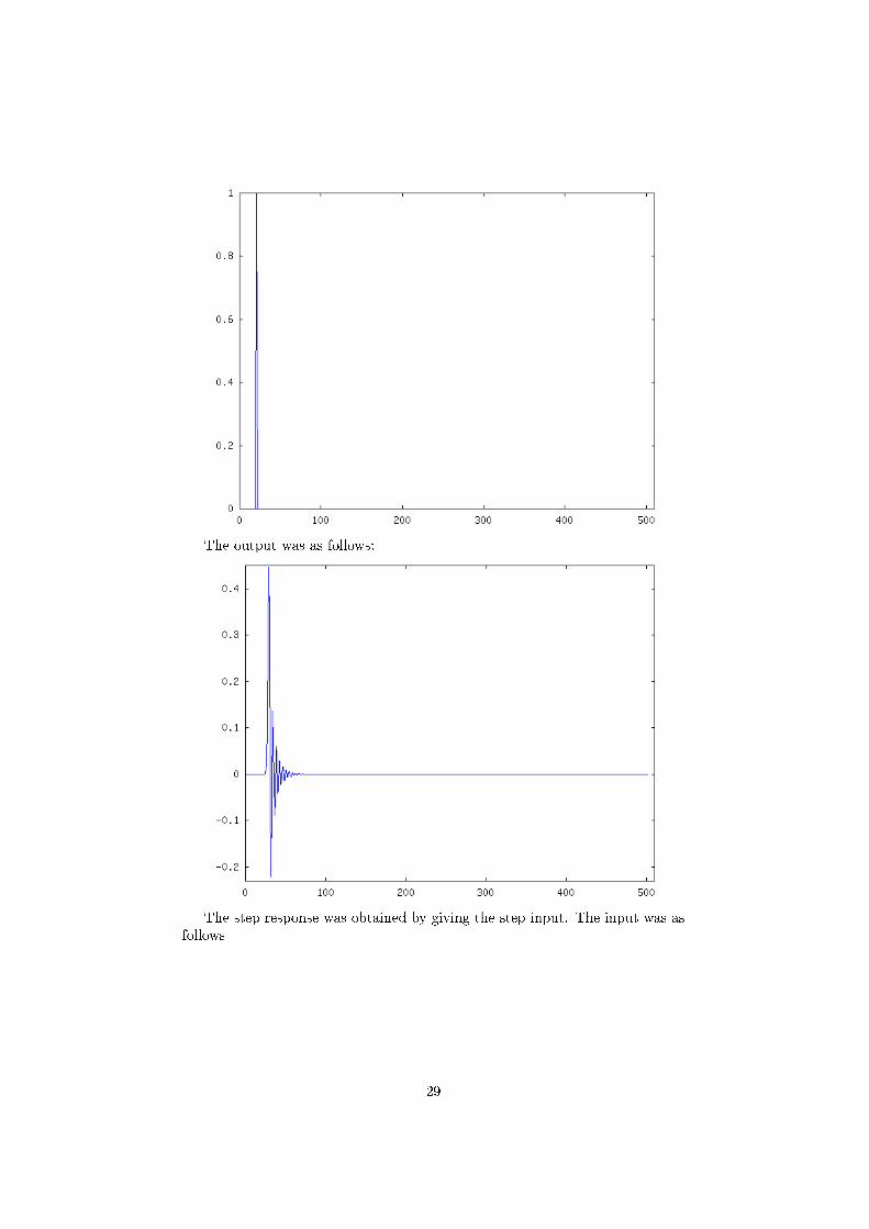
The output was as follows:

The step response was obtained by giving the step input. The input was asfollows

29

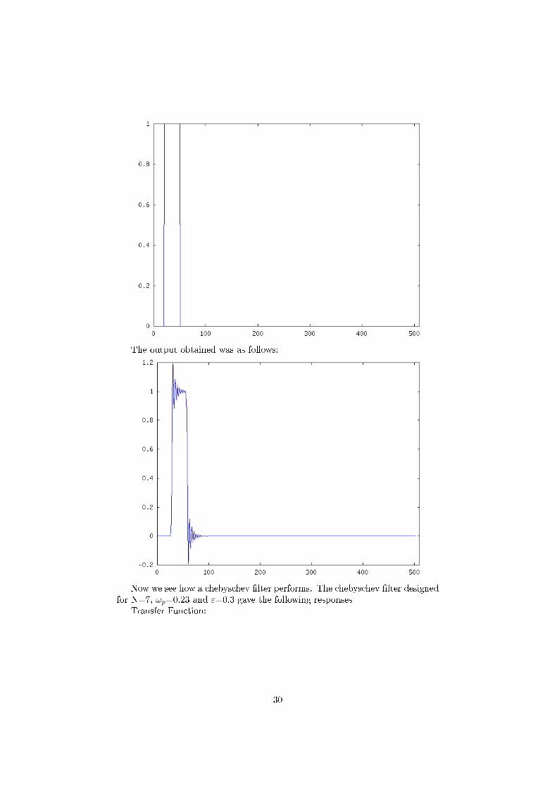
The output obtained was as follows:

Now we see how a chebyschev lter performs. The chebyschev lter designedfor N=7, ωp=0.23 and ε=0.3 gave the following responses

Transfer Function:

30

It can be observed that ripples are present only in the pass band.Transfer Function(in dB):

The impulse response was obtained by giving the same impulse as was givenpreviously. The output obtained was as follows:

31

The step response of the system is as shown

Bilinear Transformation

The Bilinear transformation is a rst order approximation of the exact map-ping (logarithmic) between the s-plane and z-plane.

z = esT

⇒ s =1Tln(z)

32

⇒ s =2T

[z − 1z + 1

+13

(z − 1z + 1

)3 + .....]

⇒ s u2T

(z − 1z + 1

)

=> s u2T

(1− z−1

1 + z−1)

The discrete-time to continuous-time frequency mapping is given by

ωa =2Ttan(

ωT

2)

Thus the entire continuous-frequency range -∞≤ωa≤∞ is mapped onto thethe discrete frequency range -Π

T≤ ω≤ΠT .

As was the case for Impulse Invariance, we have implemented 2 lters usingBilinear Transformation.

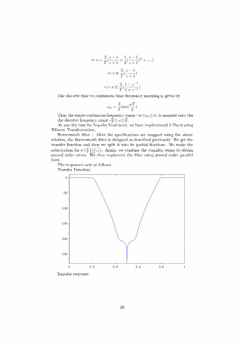
Butterworth lter : After the specications are mapped using the aboverelation, the Butterworth lter is designed as described previously. We get thetransfer function and then we split it into its partial fractions. We make the

substitution for s ( 2T

1−z−1

1+z−1 ). Again, we combine the complex terms to obtainsecond order terms. We then implement the lter using second order parallelform.

The responses were as followsTransfer Function:

Impulse response:

33

Step response:

For chebychev, as in butterworth, the specications were mapped accord-ingly and the lter was designed.

Transfer Function:

34

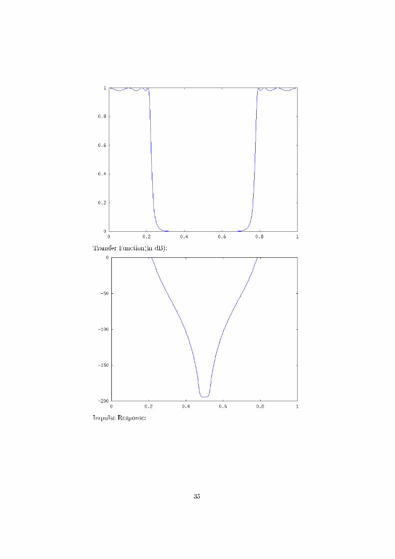
Transfer Function(in dB):

Impulse Response:

35

Step Response:

We have included only a few sample programs here, as most of the programsare very similar. We are including the bilinear tranformation butterworth andimpulse invariance butterworth lters.

Butterworth Bilinear Tranformed lter:

%N is the order of the filter and W is the cut off frequency

%specifications

36

N=14;

w=0.25;

W=2*tan(w/2);

%over

%poles

a=bpoles(N)

a=a*W*2*pi;

%splitting into residues

residues=residue1(a)

%determining n of second order filters

if rem(N,2)==0

l=(N/2)

else

l=ceil(N/2);

endif

%combining conjugate poles and transformation into z domain

final_num(1:l,1:3)=0;

final_denom(1:l,1:3)=0;

for i=1:l

if(i==N+1-i)

num=[residues(i),residues(i),0];

denom=[(2-a(i)),-2-a(i),0];

else

num=residues(i)*conv([1,1],[(2-a(N+1-i)),(-2-a(N+1-i))])+residues(N+1-i)*conv([1,1],[(2-a(i)),-2-a(i)]);

denom=linconvnormal([(2-a(i)),(-2-a(i))],[(2-a(N+1-i)),(-2-a(N+1-i))]);

endif

final_num(i,1:3)=num

final_denom(i,1:3)=denom

endfor

final_num(1:l,1:3)=(2*pi*W).^N*real(final_num(1:l,1:3));

final_denom(1:l,1:3)=real(final_denom(1:l,1:3));

%input

M=300;

k(1:M+2)=0;

temp(1:M+2)=0;

x(1:20)=0;

x(21:50)=1;

x(51:M+2)=0;

figure

plot(x);

37

%second order filters ( in parallel)

for i=1:l

for j=3:M+2

k(j)=(x(j)*final_num(i,1)+x(j-1)*final_num(i,2)+x(j-2)*final_num(i,3)-k(j-1)*final_denom(i,2)-k(j-2)*final_denom(i,3))/final_denom(i,1);

endfor

temp=temp+k;

k(1:M+2)=0;

endfor

figure

x=1:M+2;

plot(x,real(temp))

q=0:1/302:301/302

figure

plot(q,20*log(abs(fft(real(temp))))/log(10));

Butterworth Impulse Invariance Filter

%N is the order of the filter and W is the cut off frequency

%specifications

N=18;

W=0.25;

%over

%Poles are determined

a=bpoles(N)

a=a*W*2*pi;

%residues

residues=residue1(a)

%conversion to z-domain

a=exp(a);

%determining number of second order filters

if rem(N,2)==0

l=(N/2)

else

l=ceil(N/2);

endif

%combining conjugate poles

final_num(1:l,1:2)=0;

final_denom(1:l,1:3)=0;

for i=1:l

if(i==N+1-i)

num=[residues(i),0];

38

denom=[1,-a(i),0];

else

num=numerator([residues(i),residues(N+1-i)],[a(i),a(N+1-i)]);

denom=denominator([a(i),a(N+1-i)]);

endif

final_num(i,1:2)=num;

final_denom(i,1:3)=denom;

endfor

final_num(1:l,1:2)=(2*pi*W).^N*real(final_num(1:l,1:2));

final_denom(1:l,1:2)=real(final_denom(1:l,1:2));

%Input

M=500;

k(1:M+2)=0;

temp(1:M+2)=0;

x(1:20)=0;

x(21:50)=1;

x(51:M+2)=0;

figure

plot(x);

%secondr order parallel filter implementation

for i=1:l

for j=3:M

k(j)=x(j)*final_num(i,1)+x(j-1)*final_num(i,2)-k(j-1)*final_denom(i,2)-k(j-2)*final_denom(i,3);

endfor

temp=temp+k;

k(1:M+2)=0;

endfor

figure

x=1:M+2;

plot(x,real(temp))

q=0:1/502:501/502

figure

plot(q,20*log(abs(fft(real(temp))))/log(10));

39

References

[1] http://www.relisoft.com/science/Physics/t.html

[2] http://en.wikipedia.org/

[3] Digital Signal Processing, S.K. Mithra (FIR Filter Design)

[4] http://www.octave.org/

40