DSIM User Manual - PSIM Software

User’s Manual

DSIM Technology Co.

Chapter : -1

DSIM User’s ManualVersion 2020a

Release 2

May 2020

Copyright © 2020 DSIM Technology Co.

All rights reserved. No part of this manual may be photocopied or reproduced in any form or by any means without the writtenpermission of DSIM Technology Co.

DisclaimerDSIM Technology Co. (“DSIM Tech”) makes no representation or warranty with respect to the adequacy or accuracy of thisdocumentation or the software which it describes. In no event will DSIM Tech or its direct or indirect suppliers be liable forany damages whatsoever including, but not limited to, direct, indirect, incidental, or consequential damages of any characterincluding, without limitation, loss of business profits, data, business information, or any and all other commercial damages orlosses, or for any damages in excess of the list price for the licence to the software and documentation.

DSIM Technology Co.

Email: [email protected]: powersimtech.com

0 Chapter :

1 General Information

1.1 IntroductionDSIM is a simulation engine specifically designed for power electronics. With a ground breaking simulationengine and innovative modeling approach which fully exploits the characteristics of power electronic systems,it achieves an unprecedented and unparalleled performance. It increases the simulation speed by several ordersof magnitude compared with any existing simulation software. Moreover, its ability to simulate large convertersystems and at the same time switch transients is unique, and it makes it ideally suited for large scale powerconverter systems, high power converter systems, microgrid, and any systems that are computation intensive.

The DSIM engine is embedded in the PSIM simulation environment, and shares the same graphic userinterface. The simulation environment consists of the PSIM schematic capture, the DSIM simulation engine,and the waveform processing program SIMVIEW.

This manual covers necessary details about DSIM. The organization of this manual is as follows:

First of all, in Chapter 1, the working principles of DSIM will be briefly introduced, in terms of modeling andsimulating, so that users can have a basic understanding of the DSIM engine.

1.2 Modeling Power Electronic Systems in DSIMPower electronic systems are intrinsically hybrid dynamic systems composed of continuous states and discreteevents. Usually, continuous states include physical variables such as capacitor voltage and inductor current,while discrete events, such as switching events of semiconductor switches, lead to the transition of the systemfrom one operating mode to another. In power electronic systems, these continuous states and discrete eventsnot only coexist, but also deeply interact with each other and co-determine the operating mode of the system, asshown below.

Chapter 1 DSIM circuit structure, software/hardware requirement, and parameter format.

Chapter 2 Elements supported in DSIM simulation.

Chapter 3 Examples showing the performance of DSIM.

Chapter 1: General Information 1

Power electronic system is represented in DSIM in four blocks: power circuit, control circuit, sensors, andswitch controllers. The figure below shows the relationship between these blocks.

The power circuit usually consists of switching devices, RLC branches and transformers. For the switchingdevices, DSIM do not offer discrete switch elements such as a single diode, IGBT, or MOSFET, to build theconverter. Instead, switch modules such as two-level bridge leg, three-level T-type bridge leg and three-levelNPC bridge leg should be used to construct the circuit. See Elements >> Power >> Switches >> SwitchModules for all the switch modules supported in DSIM. DSIM does support bi-directional switches, but the bi-directional switch should be used for one-time event only (such as load change, open-circuit, or short-circuit). Itshould not be used for PWM operation as the DSIM engine is not optimized to handle it.

For the switching modules, two types of model are supported in DSIM, namely ideal model and transientmodel.

Ideal ModelIf ideal model is selected, DSIM will model the switch as a small resistance in on-state and as open circuit inoff-state. The on-state resistance is defined as a parameter called Switch Resistance. It is considered the samefor all the active switches and the diodes in the module. The off-state resistance is ignored. The transitionsbetween on-state and off-state are also ignored, so the system can be viewed as a piecewise-linear time-invariant (PLTI) system, which can be characterized by a set of n first-order ordinary differential equations(ODEs). Taking two-level bridge leg as an example, the figure below shows how DSIM model the switchmodule. Please refer to online help of each module to see its legal control input.

Power Circuit

Control Circuit

Sensors Switch Controllers

+

-1 2

+

-1 4

+

-1 4

Two-level bridge leg

Three-level T-type bridge leg

Three-level NPC bridge leg

2 Chapter 1: General Information

Transient ModelSwitching transients between the two steady states are sometimes significant in terms of device protection,switching loss, voltage/current balancing and EMI analysis. However, simulating switching transients in a largesystem is often challenging due to high stiffness of the circuit. DSIM adopts an innovative modeling approachcalled Piecewise Analytical Transient (PAT) model, which is capable of simulating the switching transients ina very fast and stable way. All the model parameters are available from device datasheet.

Taking a two-level bridge leg as an example, the equivalent circuit for IGBT/diode bridge and for SiCMOSFET/diode bridge is shown as below. Note that the stray inductors are already incorporated in the modelwhose values should be entered as parameters. One should not put extra stray components in the main circuitwhich will cause highly stiff equations and therefore low simulation speed.

DSIM now offers transient model for all the switching modules except three-level NPC bridges. One canchoose between IGBT/diode model and SiC MOSFET/diode model. Please turn to online help for moreinformation about the definitions of the model parameters. In Chapter 3 Examples, comparisons of the modelresults and experimental results will be presented.

The control circuit is represented in block diagram. DSIM supports only digital control temporarily.Components in z-domain, logic gates and computational blocks can be used in the control circuit. Sensors areused to measure power circuit quantities and pass them to the control circuit. Gating signals are then generatedfrom the control circuit and sent back to the power circuit through switch controllers to control switches.

The whole DSIM engine works in an event-driven manner, and one should use the switch controllers underElements >> Other >> Switch Controllers to generate switching signals. The offered components cover mostof the PWM generators including carrier-based PWM, SVPWM, square wave controller, etc. Otherwise, oneshould be careful in current DSIM version since switching events may not be located accurately.

Q1

Ls

RG

VGS

Ls

RG

VGS

Lb/2

SiC MOSFET/diode model

Lb/2

Q2

Q1RG

VGE

Lb/2

Q2RG

VGE

Lb/2

IGBT/diode model


1.3 Simulating Power Electronic Systems in DSIMDSIM engine uses a discrete state (DS) algorithm under an event-driven (ED) manner. It fully exploits thecharacteristics of power electronic systems and exhibits ultra-fast performance especially in large-scale or high-frequency systems, where typically hundred-fold acceleration can be achieved under the same accuracy,compared with existing simulation tools. Chapter 3 Examples shows some examples where such comparisonsare presented.

The DS algorithm is intrinsically a variable step-size algorithm which achieves adaptive numerical integrationof system states with less computational costs, and the ED manner avoids unnecessary iterative calculations forthe frequently-occurred switching events in power electronics. Since a variable step-size algorithm is employed,it’s not necessary for users to select a proper step-size. Instead, DSIM engine will choose the step-sizeadaptively in each calculation step. The following figure illustrates the DSIM simulation framework comparedwith the conventional one.

1.4 Installing the Program

Some of the files in the DSIM directory are:

File extensions used in DSIM are:

1.5 Simulating a Circuit To simulate the buck converter circuit “buck.dsimsch” in "examples\DSIM\dc-dc":

- Start PSIM. From the File menu, choose Open Examples..., then, go to "DSIM\dc-dc" folder to load the file “buck.psimsch”.

- From the Simulate menu, choose Run DSIM Simulation to start the simulation. Simulation results will be saved to File “buck.smv”.

- By default, Auto-run SIMVIEW is selected in the Options menu. SIMVIEW will be launched

PSIM.exe PSIM circuit schematic editor

SIMVIEW.exe Waveform processing program

*.psimsch schematic file

*.psimpjt project file

*.schpack package file

*.lib library file

*.txt Simulation output file in text format

*.smv Simulation output file in binary format

Conventional simulation framework DSIM simulation framework

4 Chapter 1: General Information

automatically. In SIMVIEW, select curves for display. If this option is not selected, from the Simulate menu, choose Run SIMVIEW to start SIMVIEW.

1.6 Simulation ControlDSIM adopts a variable-step algorithm, and users do not have to specify the simulation step. The SimulationControl element defines parameters and settings related to simulation.

To place the Simulation Control in the schematic, go to the Simulate menu, and select Simulation Control.

Image:

Some tips on how to change simulation settings:

1) Try decrease the "Relative error" if you think the simulation is not accurate enough;

2) Try decrease the "Maximum display step size" if you think the results have low resolution;

3) Try decrease the "Maximum step size" when you find that the simulation results do not converge.

End Time The total simulation time, in sec.

Maximum step size The maximum time step, in sec. If the adaptively chosen time step is larger than the "Maximum step size", the step size is forced to be "Maximum step size".

Relative error "Relative error" is used to control the numerical error in state integration. The engine chooses the step size based on "Relative error". Decreasing it leads to smaller time step, hence more accurate results but longer consuming time. In most cases, at least 1e-3 "Relative error" is recommended. One can also decrease it until no changes are observed in the simulated waveforms.

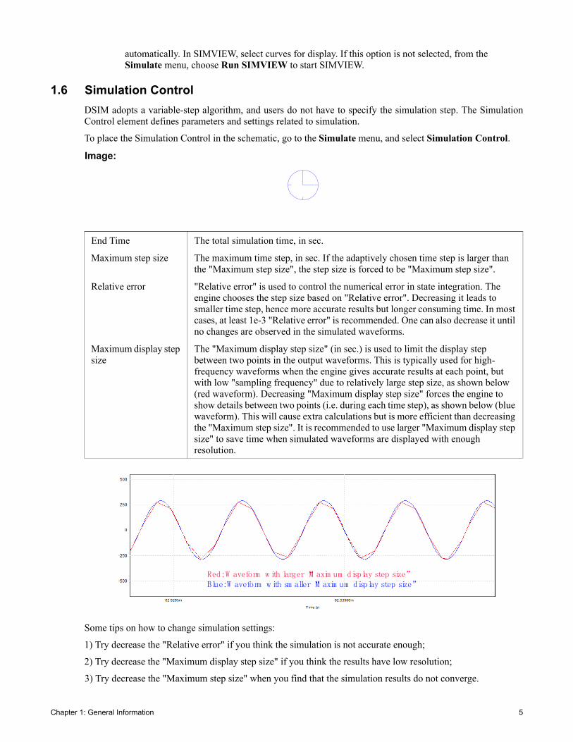
Maximum display step size

The "Maximum display step size" (in sec.) is used to limit the display step between two points in the output waveforms. This is typically used for high-frequency waveforms when the engine gives accurate results at each point, but with low "sampling frequency" due to relatively large step size, as shown below (red waveform). Decreasing "Maximum display step size" forces the engine to show details between two points (i.e. during each time step), as shown below (blue waveform). This will cause extra calculations but is more efficient than decreasing the "Maximum step size". It is recommended to use larger "Maximum display step size" to save time when simulated waveforms are displayed with enough resolution.

Red: W aveform w ith larger “M axim um display step size”Blue: W aveform w ith sm aller “M axim um display step size”


2 Elements Supported in DSIM Simulation

This chapter lists all the elements that are supported in DSIM simulation. Users can choose to display onlyDSIM supported elements in Options >> Settings >> Advanced.

The following elements are supported in DSIM.

Under Elements >> Power:

- RLC branches Resistor Inductor Capacitor Capacitor (Electrolytic) R3 L3 C3 RL3 RC3 RLC3

- Switches- Switch Modules

1-ph Inverter2-level Bridge Leg

6 Chapter 2: Elements Supported in DSIM Simulation

3-level T-Type Bridge Leg3-level NPC Bridge Leg3-ph Inverter3-ph 3-level T-Type Bridge Leg3-ph 3-level NPC BridgeDual Active Bridge (DAB)1-ph Diode Bridge3-ph Diode Bridge

- Bi-directional Switch- 3-ph Bi-directional Switch

- TransformersIdeal Transformer1-ph Transformer1-ph Transformer (no Lm)

- Renewable Energy ModuleSolar Module (physical model)

- Motor DriveSquirrel-cage Ind. Machine (with load) PMSM (with load)

*The above motor drive modules contain the following types of mechanical loads: constant torque, constantspeed, constant power, general.

Under Elements >> Control:

- Computational Blocks Multiplier

DividerSquare-rootSineSine (rad.)Sine (p.u.)ArcsineCosineCosine (rad.)Cosine (p.u.)ArccosineSine/Cosine (rad.)Sine/Cosine (p.u.)TangentArctangentArctangent (p.u.)Arctangent 2 (rad.)Arctangent 2 (p.u.)Exponential (a^x)

Chapter 2: Elements Supported in DSIM Simulation 7

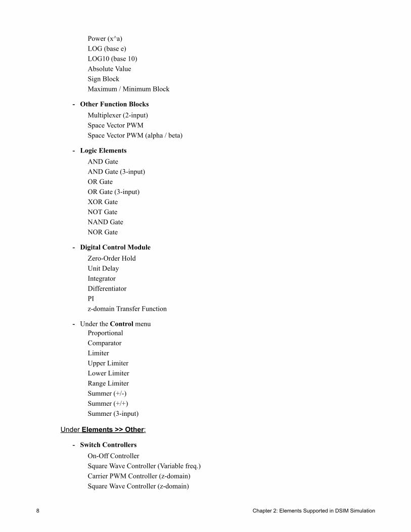
Power (x^a)LOG (base e)LOG10 (base 10)Absolute ValueSign BlockMaximum / Minimum Block

- Other Function Blocks Multiplexer (2-input)

Space Vector PWMSpace Vector PWM (alpha / beta)

- Logic ElementsAND GateAND Gate (3-input)OR GateOR Gate (3-input)XOR GateNOT GateNAND GateNOR Gate

- Digital Control ModuleZero-Order HoldUnit DelayIntegratorDifferentiatorPIz-domain Transfer Function

- Under the Control menu Proportional Comparator Limiter Upper Limiter Lower Limiter Range Limiter Summer (+/-) Summer (+/+) Summer (3-input)

Under Elements >> Other:

- Switch Controllers On-Off Controller

Square Wave Controller (Variable freq.)Carrier PWM Controller (z-domain)Square Wave Controller (z-domain)


Phase Shift Controller (z-domain)Phase Shift Controller (fixed D) (z-domain)Space Vector PWM (2-level) (z-domain)Space Vector PWM (3-level) (z-domain)

- Sensors Voltage Sensor

Current SensorVoltage Sensor (average)Current Sensor (average)

- Probes Voltage Probe

Current ProbeVoltage Probe (node-to-node)

- Function Blocks abc-dqo Transformation

dqo-abc TransformationClarke Transformation (abc-alpha/beta)Clarke Transformation (ab-alpha/beta)Clarke Transformation (ac-alpha/beta)Inverse Clarke Transformation (alpha/beta-abc)Park Transformation (alpha/beta-dq)Park Transformation (alpha/beta/sin/cos-dq)Inverse Park Transformation (dq-alpha/beta)Inverse Park Transformation (dq/sin/cos- al/be)x/y-r/angle Transformationr/angle-x/y TransformationMath FunctionMath Function (2-input)Math Function (5-input)Math Function (10-input)C BlockSimplified C Block

Under Elements >> Sources:

- Voltage DC

Sine3-ph SineGrounded Source (multiple) (constant, sine, triangular, sawtooth, square, step, step(2-level))

- Under the Sources menu:Constant

Time Ground

Chapter 2: Elements Supported in DSIM Simulation 9

Ground (1) Ground (2)


3 Examples

The high performance of DSIM and its ability to simulate switching transients makes it an ideal solution forlarge scale power converter systems, high power converter systems, microgrid, and any systems that arecomputation intensive. In this chapter, some examples are described to show how DSIM empowers the designand research of relatively complicated systems.

Example: 200kHz LLC Circuit

LLC circuit usually operates in a high-frequency range. With conventional simulation approach, very smallsimulation time step is needed to get correct results, making the whole simulation time consuming. DSIM offersan event-driven mechanism which greatly shortens the simulation time. This LLC circuit can be found underexamples >> DSIM >> LLC converter (200kHz).The following figure shows the circuit structure. The studied case is a LLC isolated bidirectional DC-DCconverter, with a variable-frequency control around 200kHz. A variable-frequency square wave controller isused to generate the switching signals. Note that for simplicity, the same switching signals are used for bothprimary and secondary side bridges. This is not the case in practice, but just an approximation to show theperformance of DSIM in similar cases.

To use an existing simulation tool with fixed step-size, a very small time step must be selected. A test result isshown in the following figure, where the simulated waveforms of the output DC voltage Vo under different timesteps are shown. It can be observed that any time step larger than 1e-9s is not enough to get correct waveforms.

Vo

400

H(z)

200k

freq

freq

0.5

0S1

S2

S4

S3

V

V

A

QD

freq

delay

Qn

Square Wave

+

-1 2

+

-1 2

+

-12

+

-12

LLC Isolated Bidirectional DC-DC Converter (8 switches, 200kHz)

Chapter 3: Examples 11

With 1e-9s time step, existing tool takes more than 20 minutes for 0.1 second simulation. However, with theDiscrete State Event-Driven algorithm, DSIM takes less than 1 second to get the same results, which is morethan 1300 times faster. The following figure shows the comparisons of the simulated results, where Vo is theoutput DC voltage, and Vcr is the resonant capacitor voltage. The tests are conducted with an Intel Core i7-6600U CPU.

Example: 50kVA Solid-State Transformer

This example shows a 50kVA solid-state transformer (SST). The system consists of three stages, as shown inthe following figure. It is tested under a 5-second grid-side low-voltage ride-through dynamic, where thewaveform of the grid-side voltage is also shown below.

0 0.02 0.04 0.06 0.08 0.1Time (s)

380

390

400

410

420

430

Vo (V

)

Discrete step=1e-7sDiscrete step=5e-8sDiscrete step=1e-8s

Discrete step 1e-8sDiscrete step 5e-9sDiscrete step 1e-9s

Existing tool

1218s (20min 18s)

0.879s

×13860 0.005 0.01 0.015 0.02 0.025 0.03 0.035390

400

410

420

Vo (V

)

0 0.005 0.01 0.015 0.02 0.025 0.03 0.035Time (s)

390

400

410

420

Vo (V

)

0 0.5 1 1.510-4

-1000

0

1000

2000

Vcr

(V)

0 0.5 1 1.5Time (s) 10-4

-1000

0

1000

2000

Vcr

(V)

Existing tool with time step 1e-9s

DSIM

Existing tool with time step 1e-9s

DSIM

Overall circuit of the 50kVA SST and simulated low-voltage ride-through dynamic

12 Chapter 3: Examples

The DSIM circuit of this example is shown below.

For the 5-second dynamic, if ideal switch model is used, DSIM takes less than 5 second to finish the simulation,which is about 50 times faster than current software; if transient switch model is used, DSIM takes about 50seconds, which is 700 times faster than another commercial software. The comparisons are shown as below.The tests are conducted with an Intel Core i7-7700K CPU.

The simulated results are in good agreements with experimental results. Some comparisons of the grid-sidewaveforms and the DC-link voltage are shown below.

The PAT model in DSIM also gives good results compared with measured ones, as shown below.

0.003 0.100

00.1e-3 9

34010e-3

10e-3300

10e-3300

1000

0.001

0.001

0.00190

50

20*sqrt(3)

sa1

sa2

sa3

sa4

sb1

sb2

sb3

sb4

sc1

sc2

sc3

sc4

ds11

ds12

ds14

ds21

ds23

ds22

ds24

s1

s2

s3

s4

ds13

50kVA Solid-State Transformer

Three-level T-Type module4kHz

DAB module20 kHz

Inverter module8kHz

+

-1 4 3 2

+ +

- -11 14 21 24

+

-sa1sb1sc1

a

b

c

Tool Device Model Solver CPU Time (s)

Software A IGBT/PiN diode: igbt_b and dp1SiC MOSFET/SiC SBD : mp1 and dp1

Trapezoidal method and Newton-Raphson iteration

33712.0(9h 21min 52s)

Software B Ideal switch model Ode23tb (Rapid mode) 250.9DSIM Transient model (PAT) DSED 47.0DSIM Ideal model DSED 4.82

×717.3×51.8

(a) grid-side voltage (b) grid-side current (c) high-voltage side DC-link voltage (d) low-voltage side DC-link voltage


Example: 10kV four-port Solid-State Transformer

This example shows how DSIM helps to simulate a very large system: a four-port solid-state transformer (SST),also known as electric energy router (EER). It consists of 576 switches in total and the rated power for each portis 1MW. The system diagram and the circuit built in DSIM is shown below.

To simulate a 0.2s dynamic, DSIM takes only 17 seconds, which is more than 1000 times faster than acommercial software specialized in power electronics, while the simulated results are very close, with less than0.01% relative error, as shown below. DSED represents the DSIM algorithm.

IGBT SiC MOSFET

iaLA

ibLA

icLA

ucn

ubn

uan

uaniaLA

Sa1

Sa2ubnibLA

Sb1

Sb2 ucnicLA

Sc1

Sc2

0Sn1Sn2

V

PWM

Qz

Vcr

Qn

+

-12

+

-12

+

-12

+

-12

10kV/2MW Electric Energy Router

HVAC

HVDC

LVDCLVAC

三相10kV交流电网

~ ~ ~

10kV直流端口

±375V直流端口

380V交流端口

~

~

~

+

-

+ -

Structure of the EER

Three-phase 10kVAC grid

10kV DC port

380VAC port

±375VDC port

Tool Configurations Number ofCalculated Points Relative Error CPU Time (s)

Software CVariable-step methodMax step-size 1e-3

Absolute tolerance 1e-4196061

Grid-side Current: 1.3e-5LVDC Transformer Current: 8.4e-5

22328(6h 12min 8s)

DSIMDSED method

Max step-size 1e-3Relative tolerance 1e-3

Grid-side Current: 7.0e-6LVDC Transformer Current: 4.7e-5 17.7101874

×1261

Simulated results comparisons of HVAC phase A grid-side current

Simulated results comparisons of LVDC output voltage

Simulated results comparisons of HVDC module 1 transformer current

-60

0

60

0.00 0.05 0.10 0.15 0.20-60

0

60

0.10010 0.10015 0.10020-44

0

44

DSED

i HD1/A

Commercial software A

t/s

i HD1/A

DSED Commercial software A

372

374

376

0.00 0.05 0.10 0.15 0.20372

374

376

0.13390 0.13395 0.13400

374.25

375.00

DSEDu LD1

/V


t/s

u LD1

/V

DSED Commercial software A

-50

0

50

0.0 0.1 0.2-50

0

50

0.13390 0.13395 0.13400-48

-45

DSED

i ga/A


t/s

i ga/A

DSED Commercial software AC

C

C

C

C C

14 Chapter 3: Examples

Example 4: Experimental Verifications of the Transient Model

This example shows the experimental verifications of the PAT model in DSIM. Double pulse tests areconducted on Infineon IGBT FZ600R65KF1 (6500V, 600A). Some experimental results are shown as below.

Generally PAT model gives good results compared with experimental waveforms, if the input parameters areaccurate enough. Under some small-current conditions, the model error can be larger.

0 1 2 3 4 5 6t/ s

0

500

1000

1500i c/A

Simulation result for icSimulation result for vceExperimental result for icExperimental result for vce

0

1000

2000

3000

v ce/V

0

1000

2000

3000

v ce/V

Switching-on signal

3000V,390A

2500V,220A

icmax Error3.88%

1.66%3.38%*1

7.44%*2

Eon Error 4.67%

Eon Error 13.20%

tr Error

*1 3000V,390A*2 2500V,220A

0 1 2 3 4 5 6t/ s

0

500

1000

1500

i c/A


0

1000

2000

3000

v ce/V

0

1000

2000

3000

v ce/V

Switching-on signal

3000V,270A

2500V,190A

icmax Error 0.99%1.65%

tr Error19.21%*1

17.32%*2

Eon Error 13.46%

Eon Error 13.37%

*1 3000V,270A*2 2500V,190A

0 2 4 6 8t/ s

0

250

500

750

1000

i c/A


0

1000

2000

3000

4000

5000

v ce/V

0

1000

2000

3000

4000

5000

v ce/V

Switching-off signal

3000V,475A

2000V,305A

vcemax Error

tf Error 6.05%

21.74%

Eoff Error 0.65%

Eoff Error 16.14%

0.28%

0.92%vcemax Error

tf Error

0 2 4 6 8t/ s

0

250

500

750

1000

i c/A


0

1000

2000

3000

4000

5000

v ce/V

0

1000

2000

3000

4000

5000

v ce/V

Switching-off signal

3000V,300A

2000V,192A

vcemax Error 3.44%

vcemax Error 4.01%Eoff Error 18.90%

Eoff Error 27.98%

tf Error

33.52%tf Error

22.72%


Documents

DSIM User Manual - PSIM Software