Revisiting the impact of the economic environment on

the shipping market: The Dry Bulk Economic Climate

Index

Vangelis Tsioumas1, Yiannis Smirlis2, Stratos Papadimitriou2 1 The American College of Greece – DEREE

2 University of Piraeus

Dr. Vangelis Tsioumas, Assistant Professor

The American College of Greece - DEREE

6 Gravias Street, Aghia Paraskevi

15342, Athens, Greece

Telephone: +30 210-600-9800 ext. 1622

etsioumas@acg.edu

Dr. Yiannis Smirlis

University of Piraeus, Greece

80, M. Karaoli & A. Dimitriou St., 18534 Piraeus

Call Centre: (+30) 210 4142000, FAX: (+30) 210 4142328

smirlis@unipi.gr

Dr. Stratos Papadimitriou, Professor

Department of Maritime Studies, University of Piraeus,

80, M. Karaoli & A. Dimitriou St., 18534 Piraeus, Greece

Call Centre: (+30) 210 4142000, FAX: (+30) 210 4142328

stratos@unipi.gr

Abstract

The present study focuses on the construction of a composite leading indicator which

is tailored to the dry cargo market and mirrors the aggregate impact of some carefully

selected economic variables. Unlike conventional approaches, the structure and the

weighting scheme of this index are based on extensive exploratory and numerical

analysis. The linkages between this new indicator and the dry bulk freight rates are

investigated by means of Co-integration analysis, Granger Causality tests and Impulse

Response analysis. Overall, the results confirm that the proposed index can successfully

narrow down the overarching impact of the economic environment and embody the

forces directed at the dry bulk freight market. Maritime practitioners may find this new

indicator particularly useful, both as a tool to gauge macroeconomic developments of

special interest and as an input to predictive models.

Keywords: Composite leading indicator; freight market; dry cargo; causality;

economic environment

1. Introduction

The exploration of the environmental context of shipping has always been a challenging

endeavour. From a systems perspective, the elements of the shipping industry interact

with the economic dimension of its general environment. The relevant literature points

out that the impact of the economic environment is ongoing, yet somewhat diffuse.

The key idea of this study is to pinpoint a set of macroeconomic factors that have a

theoretical connection with the dry bulk trade and capture their aggregate impact

through a pertinent index. This is accomplished through the construction of a new

composite indicator, which encompasses some selected economic variables and reflects

their effect on freight rates. The Dry Bulk Economic Climate Index (DBECI) is built

using only those economic variables that have a profound linkage to the freight market.

In this regard, their appropriate combination forms a leading indicator (the DBECI)

which is designed to signal economy-driven changes in the dry cargo freight market.

A major characteristic of the world economy is its cyclicality, which is compatible with

the cyclical behaviour of the shipping market (Stopford, 2009). On top of this, shipping

cycles are frequently driven by economic cycles, reflecting the close ties of the demand

for bulk carriers with the state of the economy. This cyclical process is occasionally

precipitated by random economic shocks, which usually have large-scale effects. These

rare but sudden disturbances cause substantial changes in the demand for shipping

services, affecting the level of the freight rates quite dramatically.

The high complexity of the world economy requires a painstaking process of analysing

its fundamental factors. China and the US, the world's largest economies, have a

tremendous impact on the dry bulk trade. Especially the import and export demand of

China - the leading trade nation - is a major driver of freight rates for the entire market.

From this perspective, indicators related to the world economy are not necessarily

linked to the dry bulk market, considering that they incorporate economic data of

several countries that do not trade by sea. Therefore, it is preferable to use those more

targeted metrics and thereby ensure to some extent that the sample is impervious to

outliers.

The impact of the global economy on the dry bulk freight market has been overly

evident over the course of shipping history.

The Wall Street Crash of 1929 and the subsequent great depression of 1930s set off a

prolonged shipping recession, which translated into a sharp drop of trade volume and a

large number of lay-ups.

The global economic conditions deteriorated again in 1997, due to the crisis of the

Asian economies. The falling industrial production dragged the freight market

downwards. This lasted until 2000, when the ‘Asian crisis’ ended and the industrial

production got back on track. The improved economic fundamentals led to a long

anticipated rebound of the freight market, even though it proved short-lived.

The most notable surge of the freight market took effect between 2003 and 2007, when

the rates reached historical highs. The spurring growth of China and its associated

imports of raw materials was the main driver behind this market rally. This ceased in

the second half of 2007, when a deep financial crisis spread to the world economy and

ultimately to the shipping market, causing an unprecedented plunge of freight rates in

the second half of 2008.

The relationship between the state of the economy and the seaborne trade has been

documented numerous times in the maritime literature. Isserlis (1938) highlights the

linkage between economic cycles and freight rate movements, noting that the demand

for shipping is primarily triggered by the world economy. Platou (1970) pinpoints the

influential role of the economic environment in the dry cargo market. Specifically, the

sharp decline in the industrial production of 1958 reflected the sluggish world economy

of that period which harmed the seaborne trade of raw materials and contributed to the

falling freight rates.

Going forward, many other authors have investigated the role of macroeconomic

variables in the formation of freight rates and they conclude that the major determinants

of freight rates include global economic activity, industrial production growth, and oil

prices (Hawdon, 1978; Strandenes, 1984; Beenstock & Vergottis, 1989; 1993).

Grammenos and Arkoulis (2002) investigate the impact of world macroeconomic

factors on the stock returns of several listed shipping companies. The factors under

consideration include industrial production, oil prices, inflation, exchange rates (against

the USD), and laid up tonnage. The results reveal that laid up ships and oil prices have

a negative effect on stock returns, whilst the exchange rate is positively related to the

returns of stocks. Overall, the authors identify a strong connection between the shipping

industry and the macroeconomic environment. Dikos et al. (2006) use system dynamics

modelling and look into causality effects, so as to assess the macroeconomic factors

that drive the tanker time charter rates. They estimate the flow of supply of tonnage

through entry, exit and lay-up decisions and then they compare it with demand. Finally

from their interaction they determine the key factors that affect tanker rates. In another

study, Meenaksi (2009) attempts to specify the key determinants of ship investment

decisions using the shipping recession of 2008 as a reference.

Alizadeh and Talley (2011a) focus on microeconomic determinants of dry bulk freight

rates. They examine the effect of vessel size, age, length of lay-can, and voyage route

on rates using a system of simultaneous equations. The results indicate the existence of

significant relationships; therefore, those factors should be taken into considerations

during chartering negotiations. In another study, Alizadeh and Talley (2011b) apply a

similar methodology in the tanker market and find that the determinants of tanker rates

include the ship’s hull type (single or double hull), the age, the routes, the lay-can

duration and the deadweight (dwt) utilization ratio (cargo / dwt).

Lee (2012) moves in a different direction and examines if the global economic

conditions can have a significant effect on trade disputes. This paper bears some

relevance to the subject matter of this thesis, considering that possible trade disputes

may negatively influence the trading activities and reduce the demand for shipping

services on certain routes. Moreover, viewing this in a smaller scale, it is likely to

impede the chartering negotiations between shipowners and charterers. Tang et al.

(2013) investigate the macroeconomic determinants of shipping cycles, using the

market downturn of 1980s as a point of reference. In this reading, they pinpoint the

following macroeconomic factors: the exchange rate of USD, the crude oil price, the

inflation, and the globalization.

More recently, several authors have taken into consideration the impact of economic

factors with respect to modelling and decision making in the shipping market. For

example, Lyridis et al. (2014) develop forecasting models for the dry cargo market and

incorporate macroeconomic variables. Batrinca and Cojanu (2014), in their attempt to

specify the main drivers of the dry cargo freight market, they construct a multiple OLS

regression model and seek to detect the impact of each explanatory variable on the

freight rates. The results verify the apparent negative relationship between freight rates

and supply of ships, as well as the positive one between freight rates and demand. They

also find that the world GDP has a positive effect on freight rates. However, the model

specification needs to be checked more thoroughly, while there is no evidence that the

variables fulfil the Ordinary Least Squares (OLS) assumptions. In addition, the annual

data used are not able to capture the short-term fluctuations.

2. Conceptual Framework

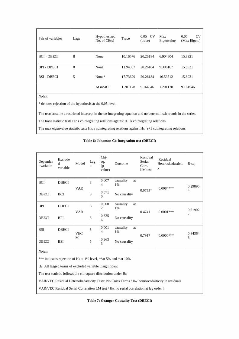
The DBECI is divided into three major components: Power of Consumers, Liquidity

and Industrial Activity. Each of them describes a separate dimension of the DBECI and

their combination shapes the final composite indicator (see Figure 1). This nested

structure reflects the conceptual formation of the composite indicator by the

aggregation of three distinct driving forces.

Insert Figure 1 about here

The ‘Power of Consumer’ component involves the following sub-indicators: New

Residential Construction (US), Euro/USD and Yuan/USD Exchange rates, and the

Brent Crude Oil Price. The ‘Liquidity’ comprises the Federal funds rate and the

Consumer Credit Outstanding (US), and lastly the ‘Industrial Activity’ component

includes the World Industrial Production and the Manufacturing and Trade Inventories

(US).

New residential construction (or Housing Starts) captures the newly issued building

permits, the new construction projects and the housing that were brought to completion.

The construction industry uses several dry bulk commodities such as steel, cement,

clinker etc. Therefore, an increase in construction activity pushes the demand for such

commodities upwards and favours the bulk carriers.

The exchange rate of Euro against the US Dollar has a significant impact on the Trans-

Atlantic trade and this extends to the entire dry cargo market. In particular, a strong

USD is seen as very expensive by European importers and this affects negatively the

US exports of dry commodities, such as grain and coal, to Europe. Likewise, the

Chinese imports from the US are significantly affected by the prevailing exchange rate.

Several authors use exchange rates as explanatory variables of shipping related metrics

(Goodwin and Schroeder (1991); Grammenos and Arkoulis, 2002; Tang et al, 2013).

Brent crude price tracks the prices of crude oil in the Atlantic and serves as a leading

benchmark for the global oil trade. The oil price is viewed as a critical determinant of

shipping freight rates by various authors (Zanettos, 1966; Beenstock and Vergottis,

1989, 1993; Grammenos and Arkoulis, 2002; Poulakidas and Joutz, 2009; Chen and

Hsu, 2012; Shi et al., 2013; Tang et al., 2013; Shen and Chou, 2015). The Brent crude

oil price is a major driver of the world economy. As oil prices fluctuate, inflation

follows suit and ultimately determines the buying power of consumers. Crude oil is a

prime source of energy and its products have various uses that range from heating and

electricity generation to their utilization as fuel in every mode of transport. Bunker fuel

prices co-fluctuate with crude oil prices; therefore higher oil prices equal higher

transport cost. This compels shipowners to seek higher freight rates so that they can

recover the higher voyage expenses. Additionally, a possible rise in oil prices increases

the production and transport costs, and eventually it is passed on the end user through

higher product prices. Consequently, higher oil prices may translate into lower

consumer spending and as a result into sluggish trading activity and diminished demand

for raw materials.

The US federal funds rate represents a target interest rate that is set by the Federal Open

Market Committee and effectively determines the interbank borrowing. When Fed

decides to raise the rate, banks are discouraged from borrowing money and

subsequently the loan interest rates rise, disincentivizing investments and generally

reducing consumption. Some authors, such as Zanettos (1966) examine the relationship

between the London Interbank Offered Rate (LIBOR) and the time charter rates. The

present study employs the fed funds rate as a more representative indicator of the

interest rate environment. In fact it has a longer term scope, while LIBOR is based on

a questionnaire and is not fixed in advance.

Τhe Consumer Credit report monitors the consumer credit conditions, tracking the

changes in the consumer outstanding debt, as this is measured by the combination of

revolving and non-revolving credit. This variable actually expresses the availability of

credit for consumers and ultimately reflects their buying power.

World industrial production measures the industrial output in the global economy. This

includes mining, manufacturing, electricity power, and utilities. Beenstock and

Vergottis (1989, 1993) and Stopford (1999) illustrate that world industrial production

is strongly related to seaborne trade. He also provides historical evidence that falling

industrial production played a central role in harming the demand for ships. Τhe level

of industrial production is closely linked to the volume of seaborne trade of the

underlying raw materials. Therefore, a sudden drop in industrial production can spiral

the freight market downwards.

The Manufacturing and Trade Inventories and Sales (US) correspond to the aggregated

value of inventories and sales across the manufacturing, retail and wholesale sectors.

High inventory levels are associated with low demand for raw materials and subdued

trading activity. On a larger scale, it is an indication of a slowing economy that harms

the demand for raw materials and leads to the accumulation of high stockpiles. A large

chunk of the aforementioned is moved by bulkers, marking the key role of inventory

levels for the dry bulk market.

3. Data and Descriptive Statistics

The dataset of the current analysis involves monthly data and spans the period from

January 1999 to July 2014. The selection of this interval was made in view of data

availability, but it allows for a full shipping cycle.

Historical data for BCI, BPI and BSI (available from 2005 onwards) were obtained

from the Clarkson’s Research Services (CRLS) database.

Table 1 states the source of each item of the DBECI.

Insert Table 1 about here

Table 2 presents the Descriptive Statistics for each sub-indicator of the DBECI.

Insert Table 2 about here

The values presented in Table 2 suggest that certain variables, such as New Residential

Construction, Brent Crude Oil Price, Consumer Credit Outstanding, and Manufacturing

and Trade Inventories are characterized by high standard deviation, which corresponds

to great volatility.

In addition, the descriptive statistics’ results illustrate that most sub-indicators are

negatively skewed, except Manufacturing and Trade Inventories and World Industrial

Production, which are skewed to the right. According to Table 2 the sample kurtosis is

less than 3 in all cases, therefore the distribution of each variable is flatter than the

normal distribution.

4. Methodology

4.1 The Benefit-of-the-doubt (BOD) approach for aggregating and weighting

sub-indicators.

For the construction of composite indicators (CIs), several different aggregating-

weighting techniques have been employed (Melyn and Moesen, 1991; OECD, 2008).

Among them, the ‘Benefit of the doubt’ (BOD) (Cherchye et al., 2007) is an alternative

procedure, based on the Data Envelopment Analysis (DEA) (Cooper et al., 2011). BOD

has been proposed for many CI cases, as a tool to compare and rank variables in terms

of their performance. On this line of research, some indicative examples include the

Human Development Index (HDI) (Lozano and Guitierrez ,2008; Despotis, 2005), the

Technology Achievement Index (TAI) (Cherchye et al., 2008) and the Digital Access

Index (Gaaloul and Khalfallah, 2013).

BOD employs linear programming to endogenously decide on the relative contribution

of the sub-indicators by selecting the values of the weights assigned to each of them.

This method has mainly been applied for benchmarking countries. The BOD

assessment retrieves the best performing variables so as to form a benchmarking

frontier, which is then used by the other variables of the model in order to estimate their

maximum relative score. The formulation of the BOD model is as follows:

Given a set of m observations, a CI can be used to compare the performance of each

individual observation relative to the others. The values of the CI derive from the

aggregation of n individual sub-indicators ( 1 2, ,.., nX X X ), which are selected as the

principal key factors. All sub-indicators are assumed to have positive contribution to

the CI and. The CI for a given variable c is estimated as the weighted sum1

n

c i ic

i

CI w x

. The icx denotes the performance of observation c (c=1,..,m) in the indicator iX and

iw the weight assigned to that indicator. Model (1) is the BOD equivalent (OECD 2008,

p. 93) for the estimation of the maximum possible value of the composite index for a

given observation, 0c .

0 0

1

CIn

c i ic

i

Max w x

1

1, c 1,..,n

c i ic

i

CI w x m

(1)

, 1,..,iw i n

Model (1) is solved m times, one for each observation and estimates the values of the

weights iw , in the optimal way, so that the composite indicator’s values is maximized.

The second constraint bounds the values cCI for all countries with the absolute limit 1,

while the third constraint ( , 1,..,iw i n ) ensures that the weights will take non-

trivial values, larger than the positive constant ε. The BOD model (1) is often enriched

with additional weight constraints to prioritize the significance of the sub-indications.

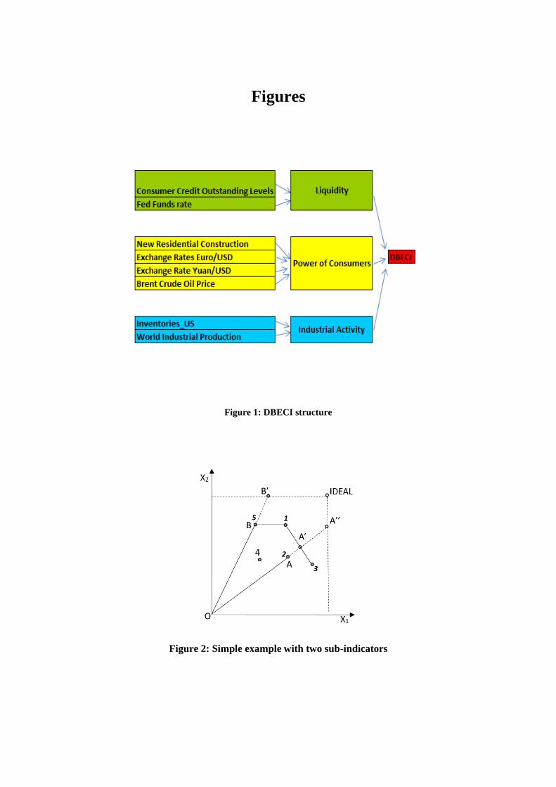
4.2 Benefit-of-the-doubt (BOD) adapted for the leading CIs.

Leading indicators are employed to predict future financial or economic trends. Unlike

typical CIs which compare a fixed, predetermined set of variables, leading indicators

are based on time series observations (months, years etc.) that continuously expand to

future periods. When considering the BOD model for the case of leading indicators, it

becomes clear that any new observation entering the system may be a potential best

performer and will consequently change the efficient frontier. Thus, due to the relative

assessment, the value of the CI for the rest of the observations may change over time

thereby making the comparison impossible. To overcome this drawback, we propose

an extension of the BOD model, which is based on the insertion of an ‘IDEAL’ virtual

observation, which is essentially a hypothetical observation having the best possible

performance. This virtual observation will dominate all existing and future units, acting

as the absolute benchmark for all time periods; thus it will make the assessment scores

unique and constant over time. This issue is demonstrated in the following simple

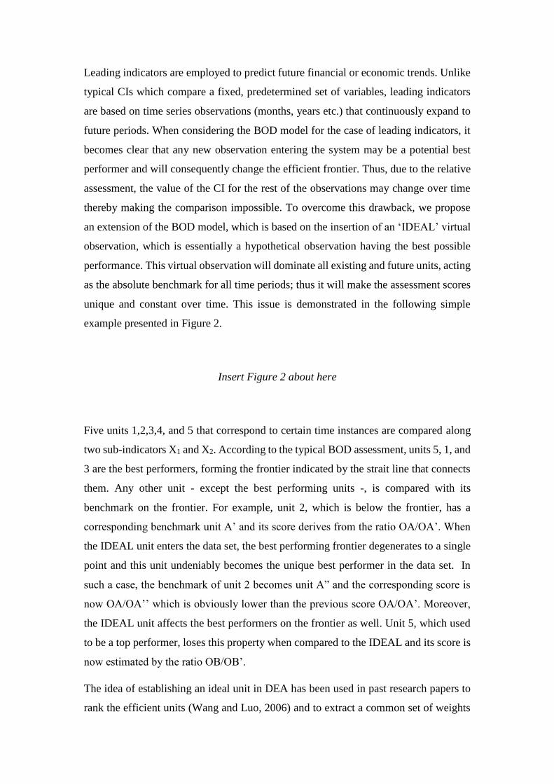
example presented in Figure 2.

Insert Figure 2 about here

Five units 1,2,3,4, and 5 that correspond to certain time instances are compared along

two sub-indicators X1 and X2. According to the typical BOD assessment, units 5, 1, and

3 are the best performers, forming the frontier indicated by the strait line that connects

them. Any other unit - except the best performing units -, is compared with its

benchmark on the frontier. For example, unit 2, which is below the frontier, has a

corresponding benchmark unit A’ and its score derives from the ratio OA/OA’. When

the IDEAL unit enters the data set, the best performing frontier degenerates to a single

point and this unit undeniably becomes the unique best performer in the data set. In

such a case, the benchmark of unit 2 becomes unit A” and the corresponding score is

now OA/OA’’ which is obviously lower than the previous score OA/OA’. Moreover,

the IDEAL unit affects the best performers on the frontier as well. Unit 5, which used

to be a top performer, loses this property when compared to the IDEAL and its score is

now estimated by the ratio OB/OB’.

The idea of establishing an ideal unit in DEA has been used in past research papers to

rank the efficient units (Wang and Luo, 2006) and to extract a common set of weights

(Payan et al., 2014). As opposed to these approaches that define the ideal unit as the

one that contains the maximum indicator values taken from the existing set of units,

according to our approach the IDEAL unit transcends any existing or possible future

observation, being the theoretical maximum value.

In the case of leading indicators the value of CI has to be estimated for m distinct time

observations t1,…,tm. Model 1 is adjusted to include the IDEAL observation and this

derives Model 2 which takes the following form:

0 0

1

CIn

t i it

i

Max w x

(2.1)

1

100, t 1,..,n

t i it

i

CI w x m

(2.2)

1

100n

ideal i iideal

i

CI w x

(2.3)

, 1,..,iw i n (2.4)

The itx and iidealx represent the values of indicator i at time t and of the IDEAL

observation respectively. The objective function (2.1) maximizes the CI value for a

given time 0t . In the constraint (2.2), without loss of generality, the upper bound 1 is

replaced by 100 for purposes of better presentation.

The inclusion of the IDEAL observation in model (2) rectifies the previously mentioned

drawbacks and generates the following properties, which significantly enhance the

model:

Property 1: Only the IDEAL can reach the maximum score of 100, i.e. 100idealCI and

all other observations at time t will have score less than 100 ( 100,tCI t )Property 2:

The score tCI of any past observation t=1,.., m remains the same when a new

observation m+1 enters the data set.

The proof of property 1 is as follows:

Since the IDEAL observation dominates all other observations in the dataset, it will

automatically reach the maximum bound, that is 100idealCI . Now assume that there

exists another observation, say 1t , that also achieves the highest score, i.e. 1

100tCI

using a specific favourite set of weights *

iw , i=1,..,n. For the observation 1t holds

1

*

1

100n

t i it

i

CI w x

. With the same set of weights, the score of the IDEAL observation

should be: 1

* *

1 1

100n n

ideal i iideal i t

i i

CI w x w x

, since by the definition of the IDEAL,

the value maxix xi,ideal is greater than any other value of the indicator i in the dataset, so

xi,ideal > xt11maxi tx x . The previous inequality 100IDEALCI CIideal > 100 contradicts

the constraint (2.3) ( 100idealCI ) and this leads to the conclusion that the hypothesis

that there exists a differeny observation from the IDEAL that achieves the maximum

score is false. Therefore, the IDEAL observation will be the unique best performer in

the dataset.

For the proof of Property 2 it is pointed out that since the IDEAL observation is the

unique benchmark observation in the dataset of the m time observations, it will also be,

by its definition, the unique benchmark in any future observation m+1, m+2, m+3 etc.

As such, it will not affect the CI score of the rest of the observations as these are only

compared to the IDEAL.

Further extending Property 2, we can conclude that for the assessment of the new time

period m+1, only the IDEAL observation is needed. This remark enables us to simplify

model (2) in terms of computational effort. Model (3) below, presents this simplified

form of model (2) by including only two observations; the new observation m+1 and

the IDEAL.

1 1

1

CIm m

n

t i it

i

Max w x

(3.1)

1 1

1

CI 100m m

n

t i it

i

w x

(3.2)

1

100n

ideal i iideal

i

CI w x

(3.3)

, 1,..,iw i n (3.4)

Model (3) can be used for the assessment of any future observation.

5. Implementation

The extended BOD model, as described in the previous sections, is applied in the case

of the new, candidate index DBCECI. DBCECI is composed of eight sub-indicators

presented in Table 1. Model (2) has been used to aggregate and weight these sub-

indicators. In this process, two additional arrangements have been made. First, in order

to prioritize the contribution of the World Industrial Production and New Residential

Construction sub-indicators to the values of the DBCECI index, the additional

constraints: 1 8 2 3 4 5 6 7, , , , , ,w w w w w w w w have been set to model (2). This is due to the

fact that these two variables have a stronger theoretical connection to seaborne trade

compared to the other sub-indicators. Second, following the lines of the BOD method,

the values ijx are normalized using the max-min rescaling formula min

max min

ij i

ij

i i

x xx

x x

,

where minix , maxix are the lowest and highest bounds respectively (see Table 2) and

correspond to the ideal point, while ijx are the new normalized values. Given that the

values ijx fall inside the interval [0..1], the ideal point is set to 1, i.e. iidealx =1. In this

respect, model (2) is run using the normalized values ijx , rather than raw data.

Insert Table 3 about here

Figure 3 presents the fluctuations of DBECI from January 1999 to July 2014. It is

worth noting that the sharp drop of DBECI before 2007 demonstrates that this leading

indicator would have been able to predict the market crash of 2007 and the subsequent

shipping market recession.

Insert Figure 3 about here

6. Validation

The next step is the exploration of potential linkages between the DBECI and the dry

cargo freight market. Considering that this relationship gives impetus to the creation

of this composite indicator in the first place, the establishment of a significant causal

relationship between DBECI and freight rates will essentially validate the role of

DBECI as a leading indicator.

Hence, the robustness of this candidate indicator is assessed by means of causality

analysis. In particular, we employ the three Baltic Exchange indices, i.e. the Baltic

Capesize Index (BCI), the Baltic Panamax Index (BPI) and the Baltic Supramax Index

(BSI), as representative indicators of the freight rate fluctuations in the dry bulk market

for three different vessel sizes.

The analysis begins with testing for unit roots using two widespread stationarity tests:

the Kwiatkowski–Phillips–Schmidt–Shin (KPSS) test and the Augmented Dickey–

Fuller (ADF) test. Both tests are carried out in the log-levels and log-differences of the

series of this analysis. The KPSS test examines the null hypothesis of stationarity under

two different assumptions: First the series have an intercept, and second, a constant and

linear trend. On the other hand, the ADF test is performed on the log- levels and log-

differences of the same variables and tests the null hypothesis of non-stationarity under

three different assumptions: An intercept, a constant and linear trend, and neither.

If the series are found non-stationary it is necessary to examine the existence of co-

integration, using the Johansen test. Then, a VAR model is developed for the levels of

the data, with the appropriate lags being determined using various lag length criteria,

such as the sequential modified LR test statistic (LR), the Final prediction error (FPE),

the Hannan-Quinn information criterion (HQ), the Schwarz information criterion (SC)

and the Akaike information criterion (AIC) (See Appendix). Thereafter, it is checked if

the model is well specified by looking at its R-squared, and by applying the VAR

Residual Serial Correlation LM test and the VAR Residual Heteroskedasticity Test.

Based on that model, the study runs Granger causality tests, as a way to investigate the

existence of causal relationships. When the results are significant, it is sensible to

proceed to Impulse Response (IR) analysis in order to explore the manner in which the

variables affect each other. In particular, IR analysis will indicate if changes in one

variable have a positive or negative effect on the other and how long this effect will

last. It should be noted that if two variables are co-integrated, the IR analysis should be

based on a VECM model and if not, on an unrestricted VAR.

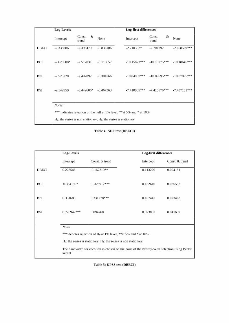
6.1 Stationarity Tests

The ADF and KPSS unit root tests are carried out in the log-levels and log-differences

of DBECI and Baltic indices. The KPSS tests the null hypothesis of stationarity under

two different assumptions: First the series have an intercept, and second, a constant and

linear trend. Alongside, the ADF test is performed on the log- levels and log-differences

of the same variables and tests the null hypothesis of non-stationarity under three

different assumptions: An intercept, a constant and linear trend, and neither.

Insert Table 4 about here

Insert Table 5 about here

The results of the ADF and KPSS tests are presented in Tables 4 and 5. The combination

of those two tests provides sufficient evidence that all series are non-stationary in level

forms, but stationary in first differences.

6.2 Co-integration Analysis

Given that the series are integrated of order 1, Johansen Co-integration test investigates

the existence of co-integrating relations. The results are presented in Table 6:

Insert Table 6 about here

The results demonstrate that there are no co-integrating relations. Therefore each pair

of variables will be modelled using an unrestricted VAR.

6.3 Causality Analysis

Insert Table 7 about here

Table 7 reports the outcome of several Granger causality tests between the BDECI and

the respective Baltic Exchange indices. It turns out that there is significant

unidirectional causality between the BDECI and each of the representative indices.

Specifically, BDECI causes BCI, BPI and BSI at a 1% level. On the flip side, there is

no causality running from any of those indices to BDECI. Therefore, this is an

indication that BDECI could be used as an exogenous variable in a freight forecasting

model.

In addition, the LM tests demonstrate that the models are free from serial correlation,

with the exception of the BCI – DBECI VAR model, which appears auto-correlated at

a high level though (10%).

Finally, even though the variables were converted into logarithmic forms, residual

heteroscedasticity is still present as shown by the relevant White heteroscedasticity tests

(no-cross terms). This may be due to the uneven distribution of the variables of this

analysis, as indicated by the skewness that the descriptive statistics of Table 1 detect.

Another possible source of heteroscedasticity is the existence of outliers, combined

with the small sample size.

In any case, although the presence of heteroscedasticity harms the efficiency of

estimators, it does not affect their consistency and unbiasedness. Hence, normally this

is not a reason to reject an otherwise satisfactory model.

6.4 Impulse Response Analysis

The next step involves IR analysis. The figures below depict the responsiveness of the

freight market to a positive shock to DBECI. Specifically, IR analysis detects the

precise reaction of each Baltic index, given a sudden spike in the DBECI.

The vertical axis measures the magnitude of the effect of the shock on each variable

and the horizontal axis the number of months after the shock.

Insert Figure 4 about here

According to Figure 4 the BCI is expected to head upwards over the short and medium

term, suggesting that a booming economic environment has a long lasting positive

impact on Capesize rates. Eventually, after some fluctuations the effect of the shock

dies out.

This behaviour is consistent with the theoretical expectations of the relationship under

consideration. Therefore, IR analysis provides empirical evidence of the direction of

the relationship between DBECI and BCI and effectively validates the utilization of the

DBECI as a leading indicator of the freight rates.

Insert Figure 5 about here

Figure 5shows the reaction of BPI to a positive shock to DBECI. The exhibit

demonstrates that the response of the BPI is quite similar to BCI. The main difference

is that in the case of Panamax vessels the full effect of the shock comes up slower, while

it dies out a little sooner and slightly more steeply. Therefore, Capesize ships are more

susceptible to changes in economic conditions, than the smaller and relatively more

versatile Panamaxes.

Insert Figure 6 about here

Finally, Figure 6 shows that BSI responds in a similar manner as the other two types of

bulk carriers. However, given that the BSI has been found co-integrated with the

DBECI, the effect of the shock does not die out. On the contrary, the two variables

reach a long-term equilibrium emanating from their co-integrating relation.

7. Conclusions

The construction of the DBECI intends to summarize several dimensions of the

economic environment that surrounds the dry cargo market. Within this framework, the

proposed indicator aims to synthesize various economic factors and capture their

aggregate influence on the dry market. Specifically, the DBECI encompasses three

distinct sub-groups of variables, with each of them reflecting a separate dimension of

the impact of the economic environment on the freight market.

The aggregation of different individual indicators into a common composite indicator

requires sound theoretical and quantitative analysis. Thus, the first step involves the

development of the theoretical framework, which dictates the selection process of the

underlying variables and explains their relevance to the dry bulk freight market.

Following the identification of the most representative macroeconomic variables, the

present study adopts a modification of a linear programming method (the ‘Benefit of

the Doubt approach’), with the purpose of assigning appropriate weights to each sub-

indicator and synthesizing them. This enhances the credibility of the proposed index

and allows its linkage with the dry bulk freight market. The latter is confirmed through

a series of pertinent statistical tests. In particular, the empirical analysis provides

evidence that there is significant causality between the DBECI and each of the Baltic

Exchange indices under consideration. In addition, the Impulse Response analysis

indicates that the DBECI has a positive short-term effect on freight rates.

Overall, it turns out that the construction of a new composite index tailored to the dry

bulk freight market sheds some light on the relationship between the freight market and

its economic environment, and opens new avenues for research.

References

Alizadeh, A. H., & Talley, W. K. (2011a). Microeconomic determinants of dry bulk

shipping freight rates and contract times. Transportation, 38(3), 561-579.

Alizadeh, A. H., & Talley, W. K. (2011b). Vessel and voyage determinants of tanker

freight rates and contract times. Transport Policy, 18(5), 665-675.

Batrinca, G. I., & Cojanu, G. S. (2014). The determining factors of the dry bulk market

freight rates. Recent Advances in Economics, Management and Development, 109.

Beenstock, M., & Vergottis, A. (1989). An econometric model of the world tanker

market. Journal of Transport Economics and Policy, 263-280.

Beenstock, M., & Vergottis, A. (1993). Econometric modelling of world shipping.

Springer Science & Business Media.

Chen, S. S., & Hsu, K. W. (2012). Reverse globalization: Does high oil price volatility

discourage international trade?. Energy Economics, 34(5), 1634-1643.

Cherchye, L., Moesen, W., Rogge, N., & Van Puyenbroeck, T. (2007). An introduction

to ‘benefit of the doubt’composite indicators. Social Indicators Research, 82(1), 111-

145.

Cherchye, L., Moesen, W., Rogge, N., Van Puyenbroeck, T., Saisana, M., Saltelli, A.,

... & Tarantola, S. (2008). Creating composite indicators with DEA and robustness

analysis: the case of the Technology Achievement Index. Journal of the Operational

Research Society, 59(2), 239-251.

Cooper, W. W., Seiford, L. M., & Zhu, J. (Eds.). (2011). Handbook on data

envelopment analysis (Vol. 164). Springer Science & Business Media.

Despotis, D. K. (2005). A reassessment of the human development index via data

envelopment analysis. Journal of the Operational Research Society, 56(8), 969-980.

Dikos, G., Marcus, H. S., Papadatos, M. P., & Papakonstantinou, V. (2006). Niver lines:

a system-dynamics approach to tanker freight modeling. Interfaces, 36(4), 326-341.

Gaaloul, H., & Khalfallah, S. (2014). Application of the “Benefit-Of-the-Doubt”

Approach for the Construction of a Digital Access Indicator: A Revaluation of the

“Digital Access Index”. Social indicators research, 118(1), 45-56.

Goodwin, B. K., and Schroeder, T. C. (1991) Price dynamics in international wheat

markets. Canadian Journal of Agricultural Economics/Revue canadienne

d'agroeconomie, 39(2), 237-254.

Grammenos, C. T., & Arkoulis, A. G. (2002). Macroeconomic factors and international

shipping stock returns. International Journal of Maritime Economics, 4(1), 81-99.

Hawdon, D. (1978). Tanker freight rates in the short and long run. Applied

Economics, 10(3), 203-218.

Isserlis, L. (1938). Tramp shipping cargoes, and freights. Journal of the Royal

Statistical Society, 101(1), 53-146.

Lee, J. E. (2012). Macroeconomic determinants of the world trade disputes. Applied

Economics, 44(33), 4301-4311.

Lozano, S., & Gutierrez, E. (2008). Data envelopment analysis of the human

development index. International Journal of Society Systems Science, 1(2), 132-150.

Lyridis, D. V., Manos, N. D., & Zacharioudakis, P. G. (2014). Modeling the Dry Bulk

Shipping Market using Macroeconomic Factors in addition to Shipping Market

Parameters via Artificial Neural Networks. International journal of transport

economics, 41(2), 231-254.

Meenaksi, B. (2009). The Impacts of the Global Crisis 2008–2009 on Shipping

Markets: A Review of Key Factors Guiding Investment Decisions in Ships. World

Maritime University Dissertations, Paper, 212.

Melyn, W., & Moesen, W. (1991). Towards a synthetic indicator of macroeconomic

performance: unequal weighting when limited information is available. Public

Economic Research Paper, 17.

Joint Research Centre-European Commission. (2008). Handbook on constructing

composite indicators: Methodology and User guide. OECD publishing.

Payan, A., Noora, A. A., & Lotfi, F. H. (2014). A Ranking Method Based on Common

Weights and Benchmark Point. Applications & Applied Mathematics, 9(1).

Platou, R.S. (1970) A survey of the tanker and dry cargo markets 1945–70. Supplement

published by Norwegian Shipping News, 10c.

Poulakidas, A., & Joutz, F. (2009). Exploring the link between oil prices and tanker

rates. Maritime Policy & Management, 36(3), 215-233.

Shen, C. W. & Chou, C. C. (2015). Temporal causality between dry bulk freight and

crude oil price. International Association of Maritime Economists (IAME) conference,

Kuala Lumpur, Malaysia

Shi, W., Yang, Z., & Li, K. X. (2013). The impact of crude oil price on the tanker

market. Maritime Policy & Management, 40(4), 309-322.

Stopford, M. (2009). Maritime Economics 3e. Routledge.

Strandenes, S. P. (1984). Price determination in the time charter and second hand

markets. Center for Applied Research, Norwegian School of Economics and Business

Administration, working paper MU, 6.

Tang, Y. X., Koh, H. L., Heng, Y. L., Soh, Z. K., & Lim, J. S. W. (2013). Shipping

cycle: factors affecting it. Singapore Maritime Academy (SMA).

Wang, Y. M., & Luo, Y. (2006). DEA efficiency assessment using ideal and anti-ideal

decision making units. Applied Mathematics and Computation, 173(2), 902-915.

Zannetos, Z. S. (1966). The theory of oil tankship rates. Massachusetts Institute of

Technology.

Tables

Indicator Data Source

x1 New Residential Construction (US) U.S. Census Bureau

x2 Exchange Rate Euro/USD Eurostat

x3 Exchange Rate Yuan/USD

Global Economic Monitor (GEM)

(World Bank Group)

x4 Brent Crude Oil Price

Clarkson Shipping Intelligence Network

x5 Federal Funds Rate

Board of Governors of the Federal

Reserve System

x6 Consumer Credit Outstanding (Levels) (US)

Board of Governors of the Federal

Reserve System

x7 Manufacturing and Trade Inventories (US) U.S. Census Bureau

x8 World Industrial Production Global Economic Monitor (GEM)

(World Bank Group)

Table 1: The eight sub-indicators of the DBECI index

Sub-Indicators

Statistic x1 x2 x3 x4 x5 x6 x7 x8

Mean 1355.04 1.22 7.48 63.36 2.25 2336883.82 1028734.88 1337.01

Median 1552 1.28 7.90 59.16 1.73 2434197.59 1022219.00 1340.00

Variance 295424.59 0.03 0.71 1221.50 4.72 2.18E+11 3.39E+10 29132.92

Std.

Deviation 543.53 0.18 0.84 34.95 2.17 467178.32 184228.75 170.68

Minimum 513 0.85 6.05 10.25 0.07 1431200.00 674466.00 1020.00

Maximum 2263 1.58 8.28 137.19 6.54 3233200.00 1400400.00 1710.00

Interquartile

Range 931 0.28 1.54 72.47 4.47 701606.50 328271.00 300.00

Skewness -0.11 -

0.52

-

0.38 0.28 0.54 -0.22 0.19 0.06

Kurtosis -1.41 -

0.68

-

1.58 -1.32

-

1.24 -0.88 -1.14 -1.16

Table 2: Descriptive statistics

minix maxix

x1 New Residential Construction (US) 200 3000

x2 Exchange Rate Euro/USD 0.5 2

x3 Exchange Rate Yuan/USD 2 15

x4 Brent Crude Oil Price 5 210

x5 Federal Funds Rate 0.01 10

x6 Consumer Credit Outstanding (Levels) (US) 950000 4200000

x7 Manufacturing and Trade Inventories (US) 500000 1750000

x8 World Industrial Production 900 2700

Table 3: Lower and Upper bounds used for max-min rescaling.

Log-Levels Log-first differences

Intercept Const. & trend

None Intercept Const. & trend

None

DBECI -2.338886 -2.395470 -0.836106 -2.710362* -2.704792 -2.658569***

BCI -2.620608* -2.517031 -0.113657 -10.15873*** -10.19775*** -10.18645***

BPI -2.525228 -2.497892 -0.304766 -10.84987*** -10.89695*** -10.87895***

BSI -2.142959 -3.442606* -0.467363 -7.410905*** -7.415576*** -7.437151***

Notes:

*** indicates rejection of the null at 1% level, **at 5% and * at 10%

H0: the series is non stationary, H1: the series is stationary

Table 4: ADF test (DBECI)

Log-Levels Log-first differences

Intercept Const. & trend Intercept Const. & trend

DBECI 0.228546 0.167210** 0.113229 0.094181

BCI 0.354190* 0.328912*** 0.152610 0.035532

BPI 0.331683 0.331278*** 0.167447 0.023463

BSI 0.770942*** 0.094768 0.073853 0.041639

Notes:

*** denotes rejection of H0 at 1% level, **at 5% and * at 10%

H0: the series is stationary, H1: the series is non stationary

The bandwidth for each test is chosen on the basis of the Newey-West selection using Berlett

kernel

Table 5: KPSS test (DBECI)

Pair of variables Lags Hypothesized No. of CE(s)

Trace 0.05 CV (trace)

Max Eigenvalue

0.05 CV (Max Eigen.)

BCI - DBECI 8 None 10.16576 20.26184 6.904804 15.8921

BPI - DBECI 8 None 11.94067 20.26184 9.306167 15.8921

BSI - DBECI 5 None* 17.73629 20.26184 16.53512 15.8921

At most 1 1.201178 9.164546 1.201178 9.164546

Notes:

* denotes rejection of the hypothesis at the 0.05 level.

The tests assume a restricted intercept in the co-integrating equation and no deterministic trends in the series.

The trace statistic tests H0: r cointegrating relations against H1: k cointegrating relations.

The max eigenvalue statistic tests H0: r cointegrating relations against H1: r+1 cointegrating relations.

Table 6: Johansen Co-integration test (DBECI)

Dependent variable

Exclude

d variable

Model Lags

Chi-

sq.

(p-value)

Outcome

Residual

Serial

Corr. LM test

Residual

Heteroskedasticity

R-sq.

BCI DBECI

VAR

8 0.007

4

causality at

1% 0.0755*

0.0084*** 0.298954

DBECI BCI 8 0.5710

No causality

BPI DBECI

VAR

8 0.0002

causality at 1%

0.4741 0.0001*** 0.219027

DBECI BPI 8 0.625

6 No causality

BSI DBECI VEC

M

5 0.0014

causality at 1%

0.7917 0.0000*** 0.34364

8 DBECI BSI 5

0.2633

No causality

Notes:

*** indicates rejection of H0 at 1% level, **at 5% and * at 10%

H0: All lagged terms of excluded variable insignificant

The test statistic follows the chi-square distribution under H0

VAR/VEC Residual Heteroskedasticity Tests: No Cross Terms / H0: homoscedasticity in residuals

VAR/VEC Residual Serial Correlation LM test / H0: no serial correlation at lag order h

Table 7: Granger Causality Test (DBECI)

Figures

Figure 1: DBECI structure

Figure 2: Simple example with two sub-indicators

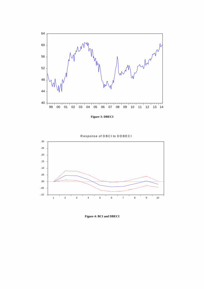
Figure 3: DBECI

Figure 4: BCI and DBECI

40

44

48

52

56

60

64

99 00 01 02 03 04 05 06 07 08 09 10 11 12 13 14

-.10

-.05

.00

.05

.10

.15

.20

.25

.30

1 2 3 4 5 6 7 8 9 10

R e s p o n s e o f D B C I t o D D B E C I

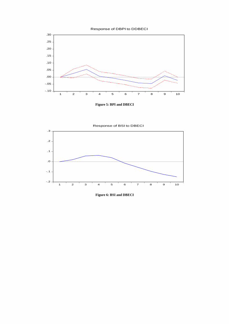
Figure 5: BPI and DBECI

Figure 6: BSI and DBECI

-.10

-.05

.00

.05

.10

.15

.20

.25

.30

1 2 3 4 5 6 7 8 9 10

Response of DBPI to DDBECI

-.2

-.1

.0

.1

.2

.3

1 2 3 4 5 6 7 8 9 10

Response of BSI to DBECI