eScholarship provides open access, scholarly publishingservices to the University of California and delivers a dynamicresearch platform to scholars worldwide.

California Partners for Advanced Transitand Highways (PATH)

UC Berkeley

Title:Vehicle Traction Control And its Applications

Author:Kachroo, PushkinTomizuka, Masayoshi

Publication Date:01-01-1994

Series:Research Reports

Permalink:http://escholarship.org/uc/item/6293p1rh

Keywords:Motor vehicles--Automatic control, Automobiles--Automatic control, Automobiles--Dynamics

Abstract:This paper presents a study of vehicle traction control and discusses its importance in highwayautomation. A robust control strategy is designed for slip control, which in turn controls the traction.It is shown how traction control can be used to satisfy different objectives of vehicle control. Theimportance of traction is further emphasized by comparing its performance to passive controllers ina simulation study in which an impulse-like wind disturbance is introduced. The comparative studyshows that the system under traction control is stable in the presence of external disturbances,whereas the system under passive control may become unstable in the presence of externaldisturbances.

Copyright Information:All rights reserved unless otherwise indicated. Contact the author or original publisher for anynecessary permissions. eScholarship is not the copyright owner for deposited works. Learn moreat http://www.escholarship.org/help_copyright.html#reuse

This paper has been mechanically scanned. Someerrors may have been inadvertently introduced.

CALIFORNIA PATH PROGRAMINSTITUTE OF TRANSPORTATION STUDIESUNIVERSITY OF CALIFORNIA. BERKELEY

Vehicle Traction Control andIts Applications

Pushkin KachrooMasayoshi Tomizuka

California PATH Research Paper

UCB-ITS-PRR-94-08

This work was performed as part of the California PATH Program ofthe University of California, in cooperation with the State of CaliforniaBusiness, Transportation, and Housing Agency, Department of Trans-portation; and the United States Department Transportation, FederalHighway Administration.

The contents of this report reflect the views of the authors who areresponsible for the facts and the accuracy of the data presented herein.The contents do not necessarily reflect the official views or policies ofthe State of California. This report does not constitute a standard,specification, or regulation.

March 1994

ISSN 1055-1425

Vehicle Traction Control And Its Applications

Pushkin Kachroo and Masayoshi Tomizuka

Department of Mechanical Engineering

University of California at Berkeley

Berkeley, California 94720

Abstract

Control of vehicle traction is of utmost importance in providing safety and obtaining

desired vehicle motion in longitudinal and lateral vehicle control. Vehicle traction control

systems can be designed to satisfy various objectives of a single vehicle system or a

platoon of vehicles in an automated highway system, which include assuring ride quality

and passenger comfort. Other objectives are aimed at providing desirable longitudinal and

lateral motion of the vehicles.

Vehicle traction force directly depends on the friction coefficient between road and

tire, which in turn depends on the wheel slip as well as road conditions. From control

point of view, we may influence traction force by varying the wheel slip. Wheel slip is a

nonlinear function of the wheel velocity and the vehicle velocity. In this paper, a robust

adaptive sliding mode controller is designed to maintain the wheel slip at any given value.

Different objectives of traction control, give different target slips to be followed.

Simulation study shows that longitudinal controllers, which do not take traction into account

explicitly (termed as tractionless or passive controllers), cannot handle external disturbances

well; on the other hand, longitudinal traction controllers (termed as active controllers) give

satisfactory results with the same disturbances. Simulations show how some of the vehicle

performance objectives are met by using traction controllers.

1. Introduction

Vehicle traction control can greatly improve the performance of vehicle motion and

stability by providing anti-skid braking and anti-spin acceleration. Vehicle traction control

is especially important for automated highway systems as related to longitudinal and lateral

control.

Many companies have developed and used anti-lock braking (ABS) and anti-slip

acceleration control systems [7, 111. A typical commercial ABS system is composed of

sensors, a control unit and a brake pressure modulator. In the prediction stage, the control

logic of such a system uses information from the wheel angular velocity and/or acceleration

to estimate the wheel slip. Wheel slip is a nonlinear function of wheel angular velocity and

vehicle velocity and is described in more detail in section-2. The control command is based

on the estimated slip and wheel acceleration. The wheel slip/acceleration phase plane is

divided into different sectors. Each sector has a corresponding control action (e.g.

APPLY, HOLD, RELEASE). This design process tries to produce an optimal limit cycle

in the phase plane of wheel slip and acceleration. The control stage of the algorithm is

usually referred to as the selection stage. Similar algorithms are designed for anti-spin

acceleration. Although these systems work in practice, their design is experimental rather

than analytical, and their tuning and calibration rely on trial and error. With the recent

advances in sensor technology [2], controllers can be designed to maintain a specified

wheel slip.

In the context of highway automation as it relates to the California Program on

Advanced Technology for Highways (PATH), we can use an alternate method to estimate

wheel slip. As angular wheel velocity is measured directly, we only need vehicle velocity to

estimate slip. For lateral control of vehicles in the PATH program, magnetic markers are

3

installed on the road at specified distances from each other in the longitudinal directions.

Vehicle velocity can thus be estimated by measuring the time elapsed between consecutive

markers.

Another method to estimate the vehicle velocity would be to use an accelerometer.

Accelerometers measure acceleration which can be integrated to calculate velocity. To

avoid accumulation of integration error, the initial velocity should be updated (from wheel

angular velocity) every few seconds before acceleration or braking starts. At the initiation

of acceleration or braking, the last initial condition should be used for the integration

process. Additional hardware may also be required to reduce the accumulation of the error

due to the slope of the road.

In this paper, it is assumed that vehicle velocity and wheel angular velocity are both

available on-line by direct measurements and/or estimations.

A controller for vehicle motion should address safety and stability of the vehicle. As

a part of highway automation, longitudinal and lateral guidance of the vehicle should be

addressed. The input forces, which control the vehicle motion come from the road-tire

interaction and have two components, one in the longitudinal direction and one in the lateral

direction. The h-active force in the lateral direction depends on the cornering stiffness and

can be controlled by the steering [8,9]. The tractive force in the longitudinal direction, on

the other hand, is a nonlinear function of the wheel slip and can be controlled by

maintaining the wheel slip at some required value. The throttle and the brakes ultimately

control the longitudinal tractive force. Controlling the longitudinal traction can achieve

various control objectives while assuring ride quality and passenger comfort. A few of

these are:

(1) Maintain the fastest stable acceleration and deceleration.

(2) Obtain anti-skid braking and anti-spin acceleration.

(3) Maintain steer-ability during lateral maneuvers.

(4) Make vehicles move longitudinally in a platoon following the vehicles in front in

an automated highway system.

(5) Make a platoon of vehicles follow a desired lateral and longitudinal path

simultaneously in an automated highway system.

A vehicle system could also use different traction control algorithms at different times

after assessing which control law is appropriate at that time instant. A supervisory control

could be devised to make such decisions. For instance, in a platoon of vehicles which is

following a curved path using control law designed for objective (5), if a vehicle starts

veering out and thus creating an emergency or abnormal condition, then changing the

control law to satisfy objective (3) might prove to be a good way to solve the problem.

In the studies for longitudinal control and platooning, it is generally assumed that the

road can provide necessary forces as determined by the controller. This assumption

implies that either the vehicle is operating in a range such that the vehicle can respond using

only a tractionless control, or that a reliable traction control is in place.

The dynamics for the system are highly nonlinear and time varying, which motivates

the use of sliding mode control strategy [13] to follow a target slip. Lyapunov stability

theorem based [ 15, 161 and sliding mode based [ 17, 18, 191 controllers have been assessed

by researchers. The sliding mode controller designed for vehicle traction control is made

adaptive to reduce the control discontinuity around the switching surface of the sliding

mode. Sliding mode based scheme is also used to estimate the road tire conditions for

maximum acceleration and maximum deceleration. The main problem with sliding mode

control is the high frequency chattering across the switching surface[ 131. A boundary layer

is introduced around the switching surface and an appropriate function is used in the

controller to reduce chattering.

Tractionless controllers can become unstable in the presence of external disturbances.

Traction controllers, on the other hand, handle disturbances well. Simulations were

performed on various road conditions to compare the performances of the two types of

controllers. A simulation study was also performed to compare the effects of wind

5

disturbance on the two types of controllers for longitudinal control of vehicles. The results

of the study are given in section-10 of this paper, which confirm the advantage of using

traction control.

2. Background

To design a good controller, a representative mathematical model of the system is

needed. In this section, a mathematical model for vehicle traction control is described [S,

6, 17, 18, 191 for analysis of the system, design of control laws, and computer

simulations. Although, the model considered here is relatively simple, it retains the

essential dynamic elements of the system.

Understanding of stability is essential for design of a good control system. The

stability of the system, described in this section, is analyzed by linearizing the system

around the equilibrium point.

2.1 System Dynamics

A vehicle model, which is appropriate for both acceleration and deceleration, is

described in this sub-section. The model identifies wheel speed and vehicle speed as state

variables and wheel torque as the input variable. The two state variables in this model are

associated with one-wheel rotational dynamics and linear vehicle dynamics. The wheel

dynamics and vehicle dynamics are derived by applying Newton’s law.

2.1.1 Wheel Dynamics

The dynamic equation for the angular motion of the wheel is

& = [T, - Tb - R,F, - R,FW]/JW (1)

6

where J, is the moment of inertia of the wheel, o, is the angular velocity of the wheel, the

over dot indicates differentiation with respect to time, and the other quantities are as defined

in Table 1. The total torque acting on the wheel divided by the moment of inertia of the

wheel equals the wheel angular acceleration. The total torque consists of shaft torque from

the engine, which is opposed by the brake torque and the torque components due to the tire

tractive force and the wheel viscous friction force. The wheel viscous friction force, a

function of the wheel angular velocity, is the friction force developed on the tire-road

contact surface. The tractive force developed on the tire-road contact surface is dependent

on the wheel slip, the difference between the vehicle speed and the wheel speed, normal&d

by the vehicle speed for braking and the wheel speed for acceleration (see Eq. (2)). The

engine torque and the effective moment of inertia of the driving wheel depend on the

transmission gear shifts.

,Rw Radius of the wheel

N, Normal reaction force from the ground

T, Shaft torque from the engine

Th Brake torque

F. Tractive force

Wheel viscous friction

Table 1 Wheel Parameters

(Acceleration)

Linear portionof the curve

(Deceleration)

-1 0Wheel Slip (h)

Figure 1 A typical ~-1 Curve

Applying a driving torque or a braking torque to a pneumatic tire produces u-active

force at the tire-ground contact patch [14,20]. The driving torque produces compression at

the tire tread in front of and within the contact patch. Consequently, the tire travels less

distance than it would if it were free rolling. In the same way, when a braking torque is

applied, it produces tension at the tire tread within the contact patch and at the front.

Because of this tension, the tire travels more distance than it would if it were free rolling.

This phenomenon is referred to as the deformation slip or wheel slip [14, 17, 18, 19,201.

The adhesion coefficient p(k) is a function of wheel slip h. Figure 1 shows a typical p-h

curve. References [17, 18 and 191 are the sources for the typical curve and [8] gives a

more mathematical description of the tire model. Mathematically, wheel slip is defmed as

h=(Ow-&)/U,OfO (2)

8

where, 0~ is vehicle angular velocity defined as

(3)

which is equal to the linear vehicle velocity, V, divided by the radius of the wheel. The

variable o is defined as

O=max(0,,0,)=1

0, for 0,2 0, \\

(4)WV for ow < ov

which is the maximum of vehicle angular velocity and wheel angular velocity.

The tire tractive force is given by

where the normal tire force, N,, depends on vehicle parameters such as the mass of the

vehicle, location of the center of gravity of the vehicle, and the steering and suspension

dynamics. The adhesion coefficient, which is the ratio between the tractive force and the

normal load, depends on the road-tire conditions and the value of the wheel slip [5, 171.

For various road conditions, the curves have different peak values and slopes, as shown in

Figure 2. The adhesion coefficient-slip characteristics are influenced by operational

parameters like speed and vertical load. The average peak values for various road surface

conditions are shown in Table 2 1141.

Surface

Asphalt and concrete (dry)

I Gravel

Ice

Snow (hard packed)

I ~ ~~~ ~ -Average Peak Value

I0.8-0.9

I0.5-0.6

0.8

0.68

0.55

0.6

0.1

0.2

Table 2 Average Peak Values for Adhesion Coefficient

9

1 .o WPavement

Wet Asphalt

0 Wheel Slip (h) 1.0

Figure 2 p--h Curves for Different Road Conditions

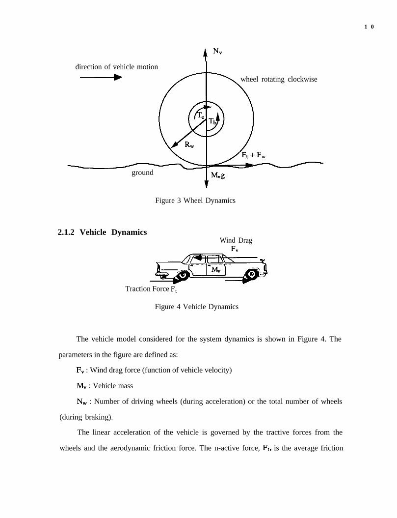
The model for wheel dynamics is shown in Figure 3. The parameters in this figure

are defined in Table 1. The figure shows the acceleration case for which the tractive force

and wheel viscous friction force are directed toward the motion. The wheel is rotating in

the clockwise motion and slipping against the ground, i.e. o, > w. The slipping produces

the n-active force towards right causing the vehicle to accelerate towards right. In the case

of deceleration, the wheel still rotates in the clockwise motion but skids against the ground,

i.e. q < %. The skidding produces the tractive force towards left causing the vehicle to

decelerate.

1 0

direction of vehicle motion

wheel rotating clockwise

ground

Figure 3 Wheel Dynamics

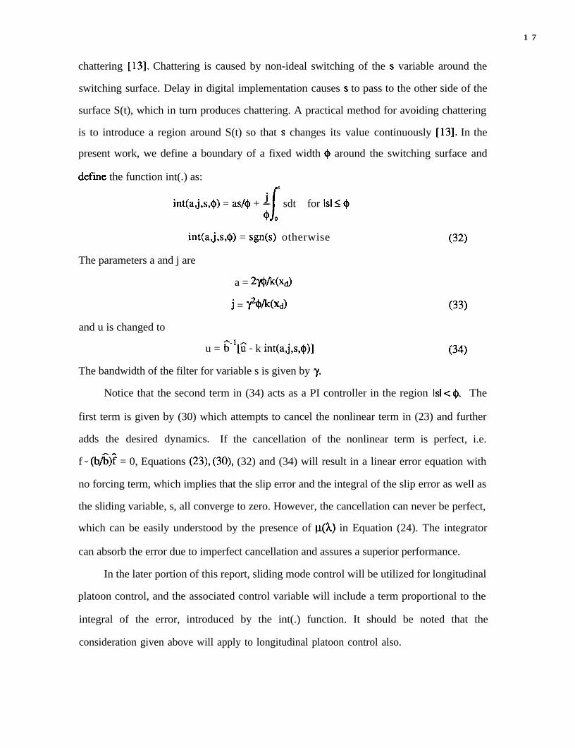
2.1.2 Vehicle DynamicsWind Drag

F”

Traction Force F,

Figure 4 Vehicle Dynamics

The vehicle model considered for the system dynamics is shown in Figure 4. The

parameters in the figure are defined as:

F, : Wind drag force (function of vehicle velocity)

M, : Vehicle mass

NW : Number of driving wheels (during acceleration) or the total number of wheels

(during braking).

The linear acceleration of the vehicle is governed by the tractive forces from the

wheels and the aerodynamic friction force. The n-active force, Ft, is the average friction

1 1

force of the driving wheels for acceleration and the average friction force of all wheels for

deceleration. The dynamic equation for the vehicle motion is

9 = [NwFt - Fv IFI, U-9

The linear acceleration of the vehicle is equal to the difference between the total tractive

force available at the tire-road contact and the aerodynamic drag on the vehicle, divided by

the mass of the vehicle. The total tractive force is equal to the product of the average

friction force, Ft and the number of relevant wheels, NW. The aerodynamic drag is a

nonlinear function of the vehicle velocity and is highly dependent on weather conditions. It

is usually proportional to the square of the vehicle velocity.

2.1.3 Combined System

The dynamic equation of the whole system can be written in state variable form by

defining convenient state variables. By defining the state variables asXl = I..

Rw (7)

x2 = 0, (8)

and denoting x = max ( x1,x2 ), we can rewrite Equations (1) and (6) as

il = -fdXd + blN CL (h > (9)

22 = -f2(x2) - b2N l.t (h ) + b3T (10)

where

T=T,-Tb

h = (x2 - x1)/x)

flh) = [Fv@wxdl/(MvRw)

blN = NvNw/(M,Rw)

f2@2) = Rw&vCQYJW

bzN = RwNv/J,

b3 = l/J, (11)

1 2

The combined dynamic system can be represented as shown in the Figure 5. The control

input is the applied torque at the wheels, which is equal to the difference between the shaft

torque from the engine and the braking torque. During acceleration, engine torque is the

primary input where as during deceleration, the braking torque is the primary input.

x = max(o, V/R,)

Figure 5 Vehicle/Brake/Road Dynamics: One-Wheel Model

2.1.4 System Dynamics In Terms Of Slip

Wheel slip is chosen as the controlled variable for traction control algorithms because

of its strong influence on the tractive force between the tire and the road. Wheel slip is

calculated from Equation (3) by using the measurements of wheel angular velocity and the

estimated value of the vehicle velocity from either the accelerometer data or the magnetic

marker data, as explained in the Introduction. By controlling the wheel slip, we control the

tractive force to obtain desired output from the system. In order to control the wheel slip, it

is convenient to have system dynamic equations in terms of wheel slip. Since the

functional relationship between the wheel slip and the state variables is different for

acceleration and deceleration, the equations for the two cases are described separately in the

following sub-sections.

1 3

Acceleration Case

During acceleration, condition x2 > xl, (x+0) is satisfied and therefore

h = (x2 - x1)/x2

Differentiating this equation, we obtain

(12)

h = [(l - h)x2 - x11/x2

Substituting Equations (9), (10) and (12) into Equation (13), we obtain

(13)

h = [ [fl(xd - (1 - %&)I - [(I - h)b;?N + blN]P + (1 - VWUh (14)

which is the wheel slip dynamic equation during acceleration. This equation is highly

nonlinear and involves uncertainties in its parameters. The non linearity of the equation is

caused by the following factors: (1) the relationship between wheel slip and wheel velocity

and vehicle velocity is nonlinear, (2) the p--h relationship is nonlinear, (3) there are

multiplicative terms like (1 - h)b&t/x2 and (1 - h&T/x2 in the equation, and (4) functions

ft(xr) and fT(x2 are nonlinear.

Deceleration Case

During deceleration, condition x2 I x1, (x1+0) is satisfied, and therefore wheel slip

is defined as:

h = (x2 - x1)/x1 (15)

Differentiating this equation, we obtain

h = [Ii2 -(l + h) ill/Xl

Substituting Equations (9), (10) and (15) into Equation (16), we obtain

(16)

h = [ [(l + h)fl(xl) - f2(x2)] - [b +(l + h) blN]jt + bJl/xl (17)

This gives the wheel slip dynamic equation for deceleration case. This equation is also

highly nonlinear and involves uncertainties like Equation (14).

1 4

2.2 SYSTEM STABILITY

The local stability of a nonlinear system can be studied by linearizing the system

around its equilibrium point. Therefore, in this section, the vehicle nonlinear system

equations are linearized around the equilibrium point in order to study the system stability.

The equilibrium point (x10,x20) of the vehicle system described by Equations (9) and (10)

can be obtained by equating the right hand sides of the two equations to zero.

Acceleration Case

For the acceleration case, the Jacobian matrix at equilibrium is:

dfl a/J- ----ho) -h--ho,x2o)/Wo,

ap(18)

dxlb1v-ho,xzo~

ah ah 40A =

I

apbN--3lOJ2O)/x20,

acL

I-~JQo~-bzN--$xlo.x2o~

x20

The eigenvalues of A are obtained by solving for h, in the equation

det&I-A) = 0 (19)

The sign of the real part of the eigenvalues determines the stability of the linearized

system. The real part of the eigenvalues is calculated to be

- ~~~~~~~~~~~~~~~~~~~~~~~~~~~~~~~~~~~[

ap

X20 12

Notice that dfl/dxl, df2/dx2, x1, x2, blN and b2N are all positive. When acl/ah is

positive, the eigenvalues of A have negative real parts, and when aCL/ah is negative, the

eigenvalues of A have positive real parts for

[ 1dfl,XlO) + df2

b&x20 + b&@ > dxl &x20)

40 CL

Hh

Hence, under the condition (20) the system is unstable.

w9

1 5

Deceleration Case

For the deceleration case, the Jacobian matrix at the equilibrium is:

A =

df 1 acL- -+x10) -bm-ho,xzo)%

dxl ah XT0

acLbm-@o,x2o~~ah XT0

(21)

L

The real part of the eigenvalues of A is calculated to bea/J

~Xlo)~Xzo)~(xlo,X2o)[blN~~N~lX10 1

2

Here also dfl/dxI, df2/dx2, x1, x2, blN and b2N are all positive, so when aCL/ah is

positive, the eigenvalues of A have negative real parts. When a@h is negative, the

eigenvalues of A have positive real parts for

+x10> + %x20)df 1x20h + bN/xlO 1 > dxl dx240 CL

Hh

(22)

Therefore, under condition (22) the system is unstable.

3. Slip Control

Longitudinal traction can be controlled by controlling wheel slip. A nonlinear control

strategy based on sliding mode, which is robust to parametric uncertainties, is chosen for

slip control.

3.1 Sliding Mode Control of the Wheel Slip

The following is the derivation of the sliding mode control law for wheel slip

1 6

regulation.

The slip dynamic equation for acceleration (13) can be written as

i=f+bu (23)

where

f = $dxl) - (1 - a)(fdXd + bi?N/@)) - bmCl(~)l

u = (l - ‘1,x2 ’

(24)

(25)

and

b = b3 (26)

Define the switching surface S(t) by equating the sliding variable, s defined below to zero.

s=h, (27)

where h, = h - & and b is the desired slip. The nonlinear function f is estimated as ‘i, and

the estimation error on f is assumed to be bounded by some known function F=F(x), so

that If - i 2 F. The control gain b is bounded as 0 5 &in I b I bmax. The control gain b

and its bounds can be time varying or state dependent. Since the control input is multiplied

by the control gain in the dynamics, the geometric mean of the lower and upper bounds of

the gain, G = V bmmbmin, is taken as the estimate of b. The bounds can also be written as

CC-~ I g/b I a, where a = 2’bmaJbmin. The controller is designed asT--=-u

(1-V (28)

where

and

u = g-‘G - k sgn(s)] (2%

G=-;+i#-J-ch, c=constant>O (30)

A finite time (I &+(0)/q) is taken to reach the switching surface and the stability of

the system is guaranteed with an exponential convergence once the switching surface is

encountered, if we choose the sliding gain as

k2a(F++)+(a-1)&l (31)

Switching control laws are known to be not prac$ical to implement because of

1 7

chattering [13]. Chattering is caused by non-ideal switching of the s variable around the

switching surface. Delay in digital implementation causes s to pass to the other side of the

surface S(t), which in turn produces chattering. A practical method for avoiding chattering

is to introduce a region around S(t) so that s changes its value continuously [13]. In the

present work, we define a boundary of a fixed width $ around the switching surface and

define the function int(.) as:

-I

t

int(a,j,s,$) = as/Q + J sdt for Isl I $4b

int(a,j,s,@) = sgn(s) otherwise (32)

The parameters a and j are

a = ~yjVWh-9

j = +W<xd, (33)

and u is changed to

u = g-‘G - k int(aj,s,+)] (34)

The bandwidth of the filter for variable s is given by ‘y.

Notice that the second term in (34) acts as a PI controller in the region Isl < 0. The

first term is given by (30) which attempts to cancel the nonlinear term in (23) and further

adds the desired dynamics. If the cancellation of the nonlinear term is perfect, i.e.

f - (bi)T = 0, Equations (23), (30), (32) and (34) will result in a linear error equation with

no forcing term, which implies that the slip error and the integral of the slip error as well as

the sliding variable, s, all converge to zero. However, the cancellation can never be perfect,

which can be easily understood by the presence of p,(h) in Equation (24). The integrator

can absorb the error due to imperfect cancellation and assures a superior performance.

In the later portion of this report, sliding mode control will be utilized for longitudinal

platoon control, and the associated control variable will include a term proportional to the

integral of the error, introduced by the int(.) function. It should be noted that the

consideration given above will apply to longitudinal platoon control also.

1 8

For deceleration, we can obtain the system in the form of Eq. (23) by defining f, u

andbas

f = [(I + h)fl(xl) - fdxdl - b2N +(I + a) hdCL]~xl (35)

u = T/xl (36)

and

b = b3 (37)

Following the same steps as for the acceleration case, the control law for deceleration is

also given by Equations (28-3 1).

3.2 Adaptive Sliding Mode Control Design

To reduce the amount of control discontinuity due to uncertainties in b, the above

described scheme can be made adaptive. It is assumed that b is a constant or a slowly

varying parameter. Adaptation is applied only outside the boundary layer so that the effect

of noise on adaptation is minimal [12]. For the system described by Eqs. (23-25), we

define

AS = s - p(.)int(a,j,s,$>, (38)

where tsdt] (39)

Notice that within the boundary, As = 0, and outside the boundary,

As = s - [Q/a]sgn(s) (40)

because the integral is reset to zero every time s goes outside the boundary. The variable a

is equated to one outside the boundary. Define a Lyapunov function candidate

(41)

Differentiating and rearranging terms, we obtain

7;1 I -qlAsl (42)

1 9

when

and

kZa(F+q) (43)

Ab&s

b (44

The adaptation law is given by Equation (44). The block diagram of the controller is

shown in Figure 6. In this figure, D refers to the Laplace operator and the dashed line

shows the adjustment of s.

-T-- ----- JI 1-1 I-- +-@ 1

- Aa

-t

I I

f

Figure 6 Block Diagram of the Traction Control

4. Optimal Time Control

The tire/road surface contact can be characterized by the local slope of the lt - h curve.

Maximum u-active force occurs at the peak of the curve where acl/ah is zero. Maximum

positive tractive force is achieved at the positive peak of the curve and is desirable in order

to achieve maximum acceleration. Maximum tractive force in the reverse direction is

achieved at the negative peak of the curve and is desired for maximum deceleration. The

2 0

acceptable operating zone for the wheel slip is between the peak slips where the slopes are

positive; outside this zone, the slopes are negative. To produce the fastest acceleration or

deceleration, which can be seen as minimum-time control, the wheel slip should be

regulated where the adhesion coefficient attains the peak value: a positive peak value for

acceleration and a negative peak value for deceleration. The derivation of this optimal

formulation is given in the appendix section of Tan’s thesis [17]. A method to estimate the

slope of the l.t - h curve, based on a single parameter sliding mode parameter estimation

scheme is described below. The algorithm is based on estimating the slope of the l.~ - h

curve and then moving the target slip in the direction of the peak slip, until the peak slip is

reached.

The minimum time acceleration and minimum time deceleration control can be

employed in a single vehicle system In an automated highway system where a platoon of

vehicles is to be controlled, minimum time acceleration and minimum time deceleration are

not generally the best performance index.

4.1 Estimation

This section explains how to use the sliding mode parameter estimation to identify the

local slope of the l.t - h curve, &./ah, from the estimations of l.t and h. In practice, the

adhesion coefficient, p,, can be regarded as a function of time (road changes) and of slip

(operating condition variations), i.e. l.t = l.t(h, t). Under the assumption that the road

condition changes either slowly or suddenly, &t/ah can be approximated by

(45)

for virtually all time instants tk, where Al.t and Ah are the differences between two adjacent

sampling instants of p and h, respectively.

To obtain the value of Ap, we differentiate Equation (9) and rearrange terms.

2 1

(46)

Since the second term inside the bracket is usually insignificant compared with the first

term, and the first term can be approximated by the difference of vehicle velocities at two

consecutive sampling time instants divided by the sample time interval, we can approximate

Ai as

Ai; = bh(tk) - ‘h(tk-I)$+--& (47)

An alternate estimation scheme could be based on differentiating Equation (10) instead of

Equation (9).

The slope is estimated by using the sliding mode parameter estimation scheme. The

parameter is updated according to

&i--$t) = -k’Ai(t)msat(a’,e,+‘) (48)

where k’ is the estimator gain and $’ is the boundary width across the switching surface.

The switching surface is described by

e = O (49)

where e is the prediction error defined asA

e=Ac-$$Ah (50)

The msat(.) function is defined as

msat(a’,e,Q’) = ale/@’ for lel < $

msat(a’,e,@) = sgn(e) otherwise (51)

This function, instead of the Signum function, is used here to reduce chattering. The

variable a’ is designed to provide a constant bandwidth filter which removes the high

frequency chattering components, by choosing

a’ = fi/[(Ai)2k’] if Ai 2 w

a’ = almax ifA^h<w (52)

where y is the desired constant bandwidth of the filter, and almax is the maximum value of

2 2

the variable a’.

4.2 Target Update Algorithm

We can utilize the sign of the current &L/&L, which is the output of the sliding mode

parameter estimation process, to reach the peak slip. This information reveals the direction

of the peak slip from the present position of h. For example, if the slope is positive at

h(tk), we know that the present slip is within the positive slope region. We therefore

propose a simple and practical method for updating the estimated peak slips based on the

sign of the estimated slope. The proposed method contains the following basic steps: (1)

Move the target slip in the estimated direction towards the peak slip. (2) Steer the wheel

slip toward the new target slip via the sliding mode slip tracking algorithm. (3) At the

same time, estimate the new local slope in the p - h curve and then return to step 1. The

algorithm designed to move the target slip toward the peak slip (step 1) is called the target

update algorithm.

The target slip is updated according to the following algorithm. The target slip is

moved in the direction of the peak according to the sign of the slope of the p - h curve.

The step size remains the same if the sign of the slope does not change, and the step size is

halved if the sign changes. The target is updated according to

GhT(k+l) = XT(k) - (-l)“sgn(%)step(k), when (-l)%(k) < 0 (53)

where,if the sign of the estimated slope at the (k+l)st instant is different from the one

estimated at the kth instant, then

step(k+l) = step(k)/2 (54)

and if the sign is same then

step(k+l) = step(k) (55)

The step size is initialized at a convenient value.

step(O) = a (56)

2 3

For varying road conditions, either the step size should have a lower bound or it should be

re-initialized if the value of the estimated slope varies substantially after a steady value has

been reached. This is important because otherwise the estimation process would cease.

Notice in Equation (53) that n = 1 is the acceleration case and n = 2 is the deceleration case.

4.3 Chattering Due To Target Updating

Chattering is observed when using the combined algorithm. This chattering should

not be confused with the sliding mode chattering for which a solution has been proposed.

This chattering is due to rapid updating of the target slip. In order to smooth the control,

the algorithm is modified such that the target is updated only when Isl c E, where s is the

sliding variable used in slip control and e is chosen to be some small positive number

which gives the desired smoothness.

5. Anti-Spin Acceleration and Anti-Skid Braking

For anti-spin acceleration and anti-skid braking, the wheel slip should be maintained

at the positive slope region of the jt- h curve. To accomplish this, we can use the

estimation scheme described in the last section. To obtain anti-spin acceleration, if the

current wheel slip is in the negative slope region, the target slip should be decremented, and

if the wheel slip is in the positive slope region, the target slip is not changed. Similarly, to

obtain anti-skid deceleration, if the current wheel slip is in the negative slope region, the

target slip should be incremented, and if the wheel slip is in the positive slope region, the

target slip is not changed.

When the aim of a traction control system is only anti-skid braking and anti-spin

acceleration without any demands on velocity or time, the ultimate control objective is not

the regulation of the wheel slip itself. The wheel slip should not enter the negative slope

2 4

region. From this point of view, a fuzzy rule-based control approach would also be

attractive and well suited.

6. Maximum Steerability in Lateral Control

Although maximum traction is desirable for optimum time control while decelerating

in straight line braking, a trade off between stability and stopping distance may be

necessary during combined hard braking and severe steering maneuvers. In these type of

maneuvers, understeered vehicles - even those equipped with ABS - will oversteer and spin

out. A previous study [15, 161 shows that for lateral control of a vehicle while

decelerating, the best cornering performance and steerability of the vehicle can be attained

by maintaining the longitudinal wheel slip at the values given by Equations (57) and (58).

The cornering performance and steerability of the vehicle is measured by the smallest

turning radius without loss of stability, combined with the shortest stopping distance.

ha = aeb16sl (57)

hrT = cedl&l (58)

In the equations, 6s is the forward steering angle; a, b, c and d are constants, the optimum

values of which can be obtained by simulations, and finally, hi and &T are the front and

the rear target slip values. These equations were obtained from analysis of simulation

results, conducted by Taheri [ 161, where different combinations of desired front and rear

slip values were used. It was found that the best combination of desired slip values, in

terms of cornering performance and steerability, could be represented by exponential

functions of the front wheel steering angle. To control the wheel slips at these values, the

traction controller designed in section 3 can be used.

2 5

7. Longitudinal Platoon Control

vehicle 2 vehicle I lead vehicle

I I direction of motion IIr-y- jqA2 4

A;, i = 1,2.. . are the spacing between consecutive vehicles

Figure 7 Platoon of vehicles

Longitudinal control strategies are necessary in order to regulate the spacing and

velocity of vehicles in an automated highway system consisting of a platoon of vehicles

(see Figure 7). The longitudinal control algorithm must maintain the spacing policy under

normal maneuvers such as acceleration, deceleration, turning, and merging. The controller

must also insure good performance over a variety of operating points and external

conditions without sacrificing safety or reliability.

The control to maintain a vehicle behind another vehicle at specified spacing in a

longitudinal platoon is obtained by using two sliding surfaces, one for tracking the vehicle

velocity, and the other to obtain the input torque. This ” two surface” method [4] is used

for systems with relative degree greater than one. The technique is discussed below.

Let s1 be the first sliding surface defined as

Sl = ti + ClE (59)

where E is the spacing error between the vehicle being controlled and the vehicle in front.

The spacing error is defined as the difference between the actual distance between the two

vehicles and the desired distance between them. When the desired distance between the

two vehicles is a constant, i: becomes the velocity error between the vehicle to be controlled

and the vehicle in front. Differentiation of Equation (59) yields

2 6

Sl = ii + Cli (60). .

where a = it - xl&s, and Xl&s is the desired xl, which is equal to the velocity of the front

vehicle for a constant desired spacing. For the first sliding surface, p(X) is the control

input, which is further controlled by the second sliding surface using the system control

input T. Using the sliding mode design procedure and introducing - ksgn(sl) term for

robustness, we obtain

$1 = il - k&s + cl& = - ksgn(sl) (61)

Substituting xl by the estimated quantities in the right hand side of Equation (9) yields

-&(x1) + i&;(h) = i&s - C1i - ksgn(sl)

From this equation, we obtain the desired adhesion value, c(h).

i(h) =& hdes +T,h> - C,i: - ksgnh)~ (63)

From the desired adhesion value, the desired slip value h&s can be calculated using the

p, - h curve. Since the actual curve is not known, we use a nominal p - h curve. The error

in the estimated and actual p value is denoted by p&h). The sliding gain of the first surface

can overcome this error by utilizing the bounds on blNj&(h). The estimated value of

ft(xl) in the Equations (62) and (63) is shown by Tl(xl). For chattering reduction, the

function sgn(.) is replaced by int(.). Here also, the control law can be made adaptive to

reduce the discontinuity across the switching surface. To obtain the desired slip, we try to

control the wheel slip directly at the desired value using the algorithm for slip-control, by

defining the second sliding surface as

s2 = h, w

The design of the control law, using the second sliding surface, is the same as described in

section 3.

In the platoon control problem, a decentralized control law is used for the special

interconnection (platoon) of the nonlinear dynamical subsystems, each one representing a

vehicle. The position errors can be obtained by integrating the velocity errors. Thus, for

2 7

each subsystem containing a vehicle in front and a following vehicle, sliding mode control

guarantees the convergence of the spacing errors with a sum of finite and exponentially

convergent time periods, so that the overall system is convergent with a rate of the slowest

dynamical subsystem.

8 Longitudinal Traction with Lateral Control

The longitudinal traction control developed in this paper can be combined with some

appropriate lateral control [8, 91 to satisfy the objective of building a complete motion

control system. In a combined platoon vehicle system for PATH, the longitudinal spacing

error between vehicles is controlled by the longitudinal controller, while the lateral

deviation and the yaw rate are controlled by the lateral controller.

It is important to use traction control when longitudinal and lateral controllers are

being implemented simultaneously, because wheel slip not only controls traction in the

longitudinal direction, but also in the lateral direction. At high wheel slip values, there is

less adhesion in the lateral direction and therefore, for lateral stability of the vehicle, the

wheel slip values should be kept low.

9 Passive Control

Some studies for longitudinal control and platooning assume that either the road can

provide necessary forces for the controller in the operating range or that a traction control is

in place. This assumption implies that if the road can react sufficiently, passive or

tractionless controllers can be used to satisfy the control objectives. Passive controllers do

not explicitly take adhesion availability of the road-tire interaction into account and therefore

their range of operation is limited as compared to the traction controllers. A simple PID

control and a sliding mode based passive control are derived next.

2 8

A simple PID control of the form

(65)

tries to minimize the longitudinal spacing error E between two vehicles without taking

traction into account. Different weights are given to the proportional, derivative and

integral terms based on experimental data. The tuning of the PID gains relies heavily on

trial and error and the design is experimental rather than analytical. Hence, there is no

stability proof for this control on the highly nonlinear model of the system.

A tractionless sliding mode controller, which tries to maintain the longitudinal spacing

between vehicles, can be designed by differentiating Equation (9), so that the input variable

appears in the equation. For instance, in the case of acceleration, we obtain

bn&(l h)x2 xl-j/x2ah - -

(66)

which can be written as

Xl = F1 + F2T (67)

where

+ blN*l il+ blN$(l _ $f2(x2) - b2NpL(h)1ahX21 ah x2

and

F2 = blN--ap (l - ‘lb,ah X2

If we let

s = i + Cl&

where & = x1 - Xl&s , the control law takes the formT = -&[-@I + xldes - cl& - k sgn(s)]

F2

(68)

(69)

(70)

(71)

where Fl is the estimate of Fl, and ^Fz is the estimate of F2. Here also sgn(.) can be

replaced by an appropriate function for chattering reduction and the sliding gain can be

chosen appropriately to ensure convergence.

29

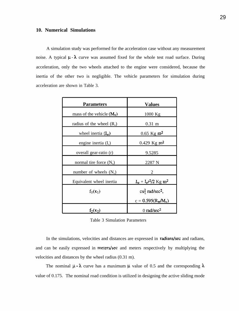
10. Numerical Simulations

A simulation study was performed for the acceleration case without any measurement

noise. A typical lo - h curve was assumed fixed for the whole test road surface. During

acceleration, only the two wheels attached to the engine were considered, because the

inertia of the other two is negligible. The vehicle parameters for simulation during

acceleration are shown in Table 3.

Parameters Values

mass of the vehicle (MV) 1000 Kg

radius of the wheel (R,) 0.31 m

wheel inertia (I,) 0.65 Kg m2

engine inertia (I,) 0.429 Kg m2

overall gear-ratio (r) 9.5285

normal tire force (N,) 2287 N

number of wheels (N,) 2

Equivalent wheel inertia IW + I,r2/2 Kg m2

flW cx! radfsec2,

c = 0.595(R,/Mv)

f2@2) 0 rad/sec2

Table 3 Simulation Parameters

In the simulations, velocities and distances are expressed in radians/set and radians,

and can be easily expressed in meters/set and meters respectively by multiplying the

velocities and distances by the wheel radius (0.31 m).

The nominal l.~ - h curve has a maximum p value of 0.5 and the corresponding h

value of 0.175. The nominal road condition is utilized in designing the active sliding mode

30

traction controller. Our intent is to simulate performance under wide varying road surface

conditions. We chose nominal road condition for the control design purposes such that the

l.~ value would be the average of the values for extreme conditions. The nominal l.~ - h

curve corresponds to an earth road. However, note that this nominal condition does not

reflect the standard highway condition. Simulations are performed on dry concrete road

and a slippery road to show extreme road conditions. It is important to analyze the

performance in the whole range of road conditions, for the presence of substances like

grease and dirt can cause the surface conditions to vary. We have chosen to use the

varying surface conditions for evaluating external disturbances, because they have a

pronounced effect on the performance of vehicles in terms of their stability. For dry

concrete road the maximum ~1 value of 0.8 is chosen and the corresponding h is 0.2,

whereas, for a slippery road, the maximum l.t value of 0.2 is chosen and the corresponding

h is 0.15. The p. - h relationship is analytically approximated by:

p = 0.3 pp A/& + A’> (72)

where l.tp represents the peak CL, and h, represents the corresponding wheel slip.

For simulations, Using Table 3, the following parameters are calculated to be

blN = 14.7548

b2N = 35.2284

b3 = 0.0497 (73)

Parametric uncertainty is taken to be about 25% for all parameters. The sampling

frequency in the simulation is 0.5 kHz.

The simulation results for the slip control (34) for desired slip equal to 0.15 are

shown in Figure 8 and Figure 9. Figure 8 shows the simulation performed on a slippery

road and Figure 9 shows the simulation performed on dry concrete. Both figures show

good wheel slip tracking in spite of 25% modeling errors in the parameters.

3 1

3 Time(sec) Time (xc)

0.05 , Sliding value vs. TimeI

i+.l.~~10 0.1 0.2 0.3

0.2 , Wheel Slip PlotI5 o.j~ 1

0 0.1 0.2 0.3Time(sec) Time (set)

Figure 8 Wheel Slip Control on a Slippery Road

5, Time Response I:w10 0.1 0.2 0.3

Time(sec) Time (set)

Controller

0 0.1 0.2 0.3

0.05 Sliding value vs. Time Wheel Slip Plot

3-3 o-

F-0.05 -25; -0.1 .

0 0.1 0.2 0.3 0 0.1 0.2 0.3Time(sec) Time (set)

Figure 9 Wheel Slip Control on Dry Concrete

32

The simulation results for the passive PID control law (65) are shown in Figure 10.

From the plot of the results, the performance is satisfactory. The disadvantage of this law

is that the gains of the controller have to be tuned based on trial and error, or by ignoring

the coupling of the two dynamic equations of the system.Time Response

0 0.1 0.2 0.3Time(sec) Time (xc)

5 Actual & Desired Velocity

3 a

2

f 0$ 0 0.1 0.2 0.3 0 0.1 0.2 0.3

Time(sec) Time (set)

Figure 10 Tractionless PID Control

Simulation results for the longitudinal traction control of a vehicle trying to maintain a

constant spacing between itself and a vehicle in front while accelerating, using the two

sliding surface method described in section-7, are shown in Figure 11 and Figure 12.

Figure 11 shows the simulation on a slippery road, while Figure 12 shows the simulation

on dry concrete. The desired adhesion in the longitudinal direction is provided by the first

sliding surface, as given by Equation (63). The torque input is computed using Equation

(34), where the second sliding surface is defined in Equation (64). The calculation of the

desired wheel slip is based on the nominal p-h curve. The actual and desired velocities

follow each other very closely even in the presence of parametric uncertainties. The

spacing errors (not shown in the plots) are however smaller than those obtained by using

3 3

the passive PID control law. Notice that wheel slip is higher on the slippery road than on

dry concrete.

3.5

3 -

Time Response

0.1 0.2Time(sec)

0.3Time (xc)

5 Actual & Desired Velocity

01 I0 0.1 0.2 0.3

Wheel Slip PlotI

Time(sec) Time (xc)

Figure 11 Longitudinal Control with Traction on a Slippery Road

3 Time(sec)

5 Actual & Desired Velocity

00 0.1 0.2

Time(sec)

0.3

1000 Controller

Fg 500-sizE 0u 0 0.1 0.2 0.3

Time (xc)

0.2 Wheel Slip Plot

0 0.1 0.2 0.3

Time (xc)

Figure 12 Longitudinal Control with Traction on Dry Concrete

34

Results of the traction control which was synthesized with the sliding mode

estimation scheme for time optimal control while accelerating a vehicle, are shown in

Figure 13 and Figure 14. Figure 13 shows the simulation on a slippery road, while Figure

14 shows the simulation on dry concrete. The peak slip for the slippery road is 0.15 and

that for dry concrete is .2. The simulation results are satisfactory as the peak slips are

followed quite well after brief transients.

Time Resnonse

5 Time(sec)

Input Torque vs. Time

0.1 0.2Time (xc)

IEstimated slope vs time

I 0.3 Wheel Slip Plot

0.1 0.2Time (set)

0.1 0.2Time (set)

Figure 13 Traction Control for Fastest Acceleration on a Slippery Road

35

Time Response Input Torque vs. TimeJ-

0.1 0.2Time(sec)

0.1 0.2Time (set)

0.3

4 Estimated slope vs time Wheel Slip Plot

2 -

0 3

0.1 0.2Time (set)

0.1 0.2Time (xc)

Figure 14 Traction Control for Fastest Acceleration on Dry Concrete

A tractionless single surface sliding mode controller (71) is used for longitudinal

control and the results are shown in Figure 15. The tracking is satisfactory.Time Response

1 2Time(sec)

8 I Actual & Desired Velocity I

0 1 2 3

600. Controller

F5 400-

$ 200-

g” 00 1 2 3

Time (set)

Wheel Slip PlotI

1 2Time (set)Time(sec)

Figure 15 Tractionless Longitudinal Control

36

Comparison of the robustness of the traction controller with tractionless controllers,

to external disturbances on a slippery road, is performed next. The combination of a

slippery road condition with a strong wind gust provides a good testing conditions for the

robustness comparison. In the longitudinal vehicle tracking while using the sliding mode

passive controller, when a wind force disturbance of 0.2g (g is the acceleration due to

gravity) is given at 0.3 seconds from the start of the simulation, for a period of 0.05

seconds, the slip becomes uncontrollable, as shown by Figure 16. The disturbance forces

the slip to attain values greater than 0.15, thereby causing it to be in the negative p - h slope

region. This makes the system unstable. Similar instability is seen in Figure 17 when the

same disturbance is given to the system, which is being controlled by the PID passive

control law, at 0.5 seconds from the start. However, using the control law with the

traction controller, as illustrated in Figure 18, the system remains stable when it encounters

the same disturbance at 0.3 seconds from the start. Although the disturbance used in these

simulations is not practical for the actual vehicle system, it gives insight into the stability of

the various longitudinal controllers during simulation.

g 100 Time Response

g

1 50-?s3 Oo 1 2 3E

$ Time(sec)

loI

Actual & Desired VelocityI

1 :_---‘i-9 0 1 2 3

Time(sec)

U -0 1 2 3Time (set)

Wheel Slip PlotI

1 2Time (set)

Figure 16 Tractionless Control with Wind Disturbance

37

Time ResponseTime Response

11 22 33Time(sec)Time(sec)

Time(sec)

Figure 17 Tractionless PJD Control with Wind Disturbance

1000 Controller

3zi 05g -looo-

8 -20000 1 2 3

Time (set)

5 Wheel Slip Plot

az-3 0-

s -50 1 2 3

Time (set)

2ooo- Controller

1000 r

O* I-y

-loo0 ;0 0.5 1 1.5

Time(sec)

Actual & Desired Velocity

Time (xc)

Wheel Slip Plot

0.5 1 1.5 0 0.5 1

Time(sec) Time (xx)

Figure 18 Traction Control with Wind Disturbance

1.5

38

11. Conclusions

It was shown that traction control is important for safety and highway automation of

vehicles. A robust control strategy was designed for slip control, which in turn controls

the traction. It was shown how traction control can be used to satisfy different objectives

of vehicle control. The importance of traction control was further emphasized by

comparing its performance to passive controllers in a simulation study in which an impulse-

like wind disturbance was introduced. The comparative study showed that the system

under traction control is stable in the presence of external disturbances, whereas the system

under passive control may become unstable in the presence of external disturbances.

Traction control can be used to enhance the performance of a single independent

vehicle with a complete set of sensors and controller integrated in a single system, or a

platoon of vehicles, where the sensors and the controllers are distributed within the vehicles

and the roadway, It can be used to accelerate or decelerate a single vehicle in the minimum

time, or it can be used to enhance the maneuvering ability of a vehicle, especially during

severe steering actions. Traction control also improves the performance of platoon of

vehicles in terms of stability and achieving a tighter control. Traction control makes the

system robust to external disturbances and provides a better control especially during

significant lateral maneuvers.

Further study of traction control is in progress including evaluation of traction control

as a part of integrated longitudinal and lateral control strategy.

12. Acknowledgments

This work was performed as part of the PATH Program of the University of

California, in cooperation with the State of California, Business and Transportation

Agency, Department of Transportation, and the United States Department of

3 9

Transportation, Federal Highway Administration.

The contents of this report reflect the views of the authors who are responsible for the

facts and the accuracy of the data presented herein. The contents do not necessarily reflect

the official views or policies of the State of California. This report does not constitute a

standard, specification, or regulation.

References

[II

PI

131

[41

[51

[61

Anderson, B. D. O., and Moore, J. B., Optimal Control-Linear Quadratic

Methods, Englewood Cliffs, NJ: Prentice Hall, 1990.

Birch, S., Vehicle Sensor, Automotive Engineering, Vol. 97, No. 6, 91-92,

June 1989

Gupta, N., Frequency-Shaped Cost Functionals: Extension of Linear-Quadratic-

Gaussian Design Method, J. Guidance and Contr., vol. 3, no. 6, pp. 529-535,

Nov.-Dec. 1980.

Green, J., and Hedrick, J. K., Nonlinear Torque Control for Gasoline Engines,

Proc. ACC, 1990.

Harned, J. L., et al., Measurement of Tire Break Force Characteristics as related

to Wheel Slip Control System Design, SAE Trans. Vol. 78, pp. 909-925, No.

690214, 1969.

Leiber, H. et al., Anti-Skid System (ABS) for Passenger Cars, Bosch Technical

and Scientific Report, Feb. 1982.

4 0

l-71 Leiber, H., and Czinczel, A., Four Years of Experience with 4-Wheel Antiskid

Brake (ABS), SAE 830481, 1983.

181 Peng, H., and Tomizuka, M., Vehicle Lateral Control for Highway Automation,

ACC Proceedings, San Diego., pp. 788-794, 1990.

r91 Matsumoto, N., and Tomizuka, M., Vehicle Lateral Velocity and Yaw Rate

Control with Two Independent Control Inputs, Trans. of the ASME , 114, pp.

606-613, 1992.

II101 Rohrs, C. E., Valavani, L. S., Athans, M., and Stein, G., Robustness of

Continuous-Time Adaptive Control Algorithms in the Presence of Unmodeled

Dynamics, IEEE Trans. on Aut. Cont., 30, pp. 881-889, 1985.

II111 Schurr, H., and Dittner, A., A New Anti-skid-Brake System for Disc and Drum

Brakes, Braking: Recent Developments, SAE 840486, May 1984.

WI Slotine, J.-J. E., and Coetsee, J. A., Adaptive Sliding Controller Synthesis for

Nonlinear Systems, Int. J. Control , 1986.

[I31 Slotine, J.-J. E., and Li, Weiping, Applied Nonlinear Control, Prentice Hall,

New Jersey, 1991.

II141 Taborek, J. J., Mechanics of Vehicle, Penton, Cleveland, 1957.

4 1

[I51 Taheri, S., A Feasibility Study of the Use of a New Nonlinear Control Law for

Automobile Anti-lock Braking Systems, ACC Proceedings, vol. 2 of 3, 1990.

[161 Taheri, S., A, and Law, E. H., Investigation of Integrated Slip Control Braking

and Closed Loop Four Wheel Steering Systems for Automobiles during

Combined Hard Braking and Severe Steering, ACC Proceedings, ~01.2, 1990.

[I71 Tan, H. S., Adaptive and Robust Controls with Application to Vehicle Traction

Control, PhD. Dissertation, University of California, Berkeley, 1988.

1181 Tan, H. S., and Tomizuka, M., A Discrete-Time Robust Vehicle Traction

Controller Design, ACC Proceedings, pp. 1053-1058, 1989.

1191 Tan, H. S., and Tomizuka, M., An Adaptive Sliding Mode Vehicle Traction

Controller Design, ACC Proceedings, vol. 2 of 3, pp. 1856-1861, 1990.

m Wong, J. Y., Theory of Ground Vehicles, Wiley, New York,, 1978.