DRELL-YAN PRODUCTION AT SMALL QT

DRELL-YAN PRODUCTION AT SMALL QT

Thomas BecherUniversity of Bern

HP2, Florence, Sept. 14-17, 2010

transverse PDFs, the collinear anomaly, and resummation at NNLL

arXiv:1007.4005 with Matthias Neubert

1

OUTLINE• Factorization of the cross section at low transverse

momentum qT

• The collinear anomaly and the definition of transverse momentum dependent PDFs

• Resummation of large log’s

• Relation to the Collins Soper Sterman (CSS) formalism

•Numerical results to NNLL

2

The production of a lepton pair with large invariant mass is the most basic hard-scattering process at a hadron collider. This is the place for HP2 at hadron colliders!

ATLAS has 3.5 pb-1 of data: ~ 7 x105 W’s and 2x105 Z’s !

[GeV]ZT

p0 20 40 60 80 100 120

Entri

es/5

GeV

0

5

10

15

20

25

[GeV]ZT

p0 20 40 60 80 100 120

Entri

es/5

GeV

0

5

10

15

20

25-1 L = 229 nb!Preliminary ATLAS

=7 TeV)sData 2010 (

µµ "Z

3

PERTURBATIVE EXPANSIONThe perturbative expansion of the qT spectrum contains singular terms of the form (M is the invariant mass of the lepton pair)

which ruin the perturbative expansion at qT ≪ M and must be resummed to all orders.

classic example of an observable which needs resummation!

4

dσ

dq2T

=1

q2T

[

A(1)1 αs ln

M2

q2T

+ αsA(1)0 + A(2)

3 α2s ln3 M2

q2T

+ . . . (1)

+A(n)2n−1α

ns ln2n−1 M2

q2T

+ . . .]

+ . . . (2)

ψγµψ → CV (M2, µ) χhc S†n γµ Sn χhc (3)

CV , anti-coll. soft coll.

p p M2 = (p − p)2 JµV

n n

(−gµν) 〈N1(p) N2(p)| Jµ†V (x) Jν

V (0) |N1(p) N2(p)〉 →1

2Nc|CV (M2, µ)|2

× WDY(x) 〈N1(p)| χhc(x)/n

2χhc(0) |N1(p)〉〈N2(p)| χhc(0)

/n

2χhc(x) |N2(p)〉

WDY(x) =1

Nc〈0|Tr

[

S†n(x) Sn(x) S†

n(0) Sn(0)]

|0〉 (4)

Sn(x) = P exp

[

i

∫ 0

−∞

ds n · As(x + sn)

]

(5)

(n · k, n · k, k⊥)

x ∼ M−1(1, 1, λ−1)

phc ∼ M (λ2, 1, λ) , phc ∼ M (1, λ2, λ) , (6)

ps ∼ M (λ2, λ2, λ2) . (7)

WDY(0) 〈N1(p)| χhc(x+ + x⊥)/n

2χhc(0) |N1(p)〉〈N2(p)| χhc(0)

/n

2χhc(x− + x⊥) |N2(p)〉

WDY(0) = 1 (8)

WDY(x0) 〈N1(p)| χhc(x+)/n

2χhc(0) |N1(p)〉〈N2(p)| χhc(0)

/n

2χhc(x−) |N2(p)〉

1

RESUMMATIONA formula which allows for the resummation of the logarithmically enhanced terms at small qT to arbitrary precision was first obtained by Collins, Soper and Sterman (CSS) in ‘84, based on earlier work of Collins and Soper.

A corresponding expression for the simpler case of soft-gluon resummation was derived only later by Sterman in ’87, and by Catani and Trentadue in ‘89.

We will now analyze the factorization properties of the cross section in these kinematic configurations.

5

FACTORIZATION6

• Starting point is the factorization of the electroweak current in the Sudakov limit

• In Soft-Collinear Effective Theory (SCET) this can be written in operator form as

SOFT-COLLINEAR FACTORIZATION dσ

dq2T

=1

q2T

[

A(1)1 αs ln

M2

q2T

+ A(1)0 + A

(2)3 α2

s ln3 M2

q2T

+ . . . (1)

+A(n)2n−1α

ns ln2n−1 M2

q2T

+ . . .]

+ . . . (2)

ψγµψ → CV (−q2− iε, µ) χhc S†

n γµ Sn χhc (3)


1

soft

hc

hc

dσ

dq2T

=1

q2T

[

A(1)1 αs ln

M2

q2T

+ A(1)0 + A

(2)3 α2

s ln3 M2

q2T

+ . . . (1)

+A(n)2n−1α

ns ln2n−1 M2

q2T

+ . . .]

+ . . . (2)



1

dσ

dq2T

=1

q2T

[

A(1)1 αs ln

M2

q2T

+ A(1)0 + A

(2)3 α2

s ln3 M2

q2T

+ . . . (1)

+A(n)2n−1α

ns ln2n−1 M2

q2T

+ . . .]

+ . . . (2)



p p M2 = (p − p)2

1

dσ

dq2T

=1

q2T

[

A(1)1 αs ln

M2

q2T

+ A(1)0 + A

(2)3 α2

s ln3 M2

q2T

+ . . . (1)

+A(n)2n−1α

ns ln2n−1 M2

q2T

+ . . .]

+ . . . (2)



p p M2 = (p − p)2

1

dσ

dq2T

=1

q2T

[

A(1)1 αs ln

M2

q2T

+ A(1)0 + A

(2)3 α2

s ln3 M2

q2T

+ . . . (1)

+A(n)2n−1α

ns ln2n−1 M2

q2T

+ . . .]

+ . . . (2)



p p M2 = (p − p)2

1

dσ

dq2T

=1

q2T

[

A(1)1 αs ln

M2

q2T

+ A(1)0 + A

(2)3 α2

s ln3 M2

q2T

+ . . . (1)

+A(n)2n−1α

ns ln2n−1 M2

q2T

+ . . .]

+ . . . (2)



p p M2 = (p − p)2 JµV

1

hard-collinear

anti-hard-collinear

SCET hc quark field

Cqq→ij(z1, z2, q2T , M2, µ) =

∣

∣CV (−M2, µ)∣

∣

2 1

4π

∫

d2x⊥ e−iq⊥·x⊥

(

x2T M2

4e−2γE

)−Fqq(x2

T ,µ)

× Iq←i(z1, x2T , µ) Iq←j(z2, x

2T , µ)

(23)

µ = µb = 2e−γE x−1⊥

µ = qT

(24)

µ = µb = 2e−γE/x⊥

A(3) = ΓF2 + 2β0d

q2 = 239.2 − 652.9 #= ΓF

2 (25)

exp(

−αscL2⊥

)

(26)

η =CFαs

πln

M2

µ2(27)

qT

L⊥

〈x−1T 〉 = q∗ = M exp

(

−π

2CF αs(q∗)

)

= 1.78 GeV for M = MZ (28)

µ = max (q∗, qT )

λ =pT

M(29)

nµ ∼pµ

p0

nµ ∼pµ

p0

4

Cqq→ij(z1, z2, q2T , M2, µ) =

∣

∣CV (−M2, µ)∣

∣

2 1

4π

∫


(

x2T M2

4e−2γE

)−Fqq(x2

T ,µ)


2T , µ)

(23)

µ = µb = 2e−γE x−1⊥

µ = qT

(24)


A(3) = ΓF2 + 2β0d

q2 = 239.2 − 652.9 #= ΓF

2 (25)

exp(

−αscL2⊥

)

(26)

η =CFαs

πln

M2

µ2(27)

qT

L⊥

〈x−1T 〉 = q∗ = M exp

(

−π

2CF αs(q∗)

)

= 1.78 GeV for M = MZ (28)


λ =pT

M(29)

nµ ∼pµ

p0

nµ ∼pµ

p0

4

7

The Drell-Yan cross section is obtained from the matrix element of two currents

and are light-cone reference vectors along and .

The soft function contains a product of four Wilson lines along the directions of large energy flow

dσ

dq2T

=1

q2T

[

A(1)1 αs ln

M2

q2T

+ A(1)0 + A

(2)3 α2

s ln3 M2

q2T

+ . . . (1)

+A(n)2n−1α

ns ln2n−1 M2

q2T

+ . . .]

+ . . . (2)



p p M2 = (p − p)2 JµV


V (0) |N1(p) N2(p)〉 →1

2Nc|CV (M2, µ)|2


2χhc(0) |N1(p)〉〈N2(p)| χhc(0)

/n

2χhc(x) |N2(p)〉

1

dσ

dq2T

=1

q2T

[

A(1)1 αs ln

M2

q2T

+ A(1)0 + A

(2)3 α2

s ln3 M2

q2T

+ . . . (1)

+A(n)2n−1α

ns ln2n−1 M2

q2T

+ . . .]

+ . . . (2)



p p M2 = (p − p)2 JµV

n n


V (0) |N1(p) N2(p)〉 →1

2Nc|CV (M2, µ)|2


2χhc(0) |N1(p)〉〈N2(p)| χhc(0)

/n

2χhc(x) |N2(p)〉

1

dσ

dq2T

=1

q2T

[

A(1)1 αs ln

M2

q2T

+ A(1)0 + A

(2)3 α2

s ln3 M2

q2T

+ . . . (1)

+A(n)2n−1α

ns ln2n−1 M2

q2T

+ . . .]

+ . . . (2)



p p M2 = (p − p)2 JµV

n n


V (0) |N1(p) N2(p)〉 →1

2Nc|CV (M2, µ)|2


2χhc(0) |N1(p)〉〈N2(p)| χhc(0)

/n

2χhc(x) |N2(p)〉

1

dσ

dq2T

=1

q2T

[

A(1)1 αs ln

M2

q2T

+ A(1)0 + A

(2)3 α2

s ln3 M2

q2T

+ . . . (1)

+A(n)2n−1α

ns ln2n−1 M2

q2T

+ . . .]

+ . . . (2)



p p M2 = (p − p)2 JµV

n n


V (0) |N1(p) N2(p)〉 →1

2Nc|CV (M2, µ)|2


2χhc(0) |N1(p)〉〈N2(p)| χhc(0)

/n

2χhc(x) |N2(p)〉

WDY(x) =1

Nc〈0|Tr

[

S†n(x) Sn(x) S†

n(0) Sn(0)]

|0〉 (4)

1

dσ

dq2T

=1

q2T

[

A(1)1 αs ln

M2

q2T

+ A(1)0 + A

(2)3 α2

s ln3 M2

q2T

+ . . . (1)

+A(n)2n−1α

ns ln2n−1 M2

q2T

+ . . .]

+ . . . (2)



p p M2 = (p − p)2 JµV

n n


V (0) |N1(p) N2(p)〉 →1

2Nc|CV (M2, µ)|2


2χhc(0) |N1(p)〉〈N2(p)| χhc(0)

/n

2χhc(x) |N2(p)〉

WDY(x) =1

Nc〈0|Tr

[

S†n(x) Sn(x) S†

n(0) Sn(0)]

|0〉 (4)

Sn(x) = P exp

[

i

∫ 0

−∞ds n · As(x + sn)

]

(5)

1

8

Final step is to expand the matrix elements in small momentum components, i.e. to perform a derivative expansion.

The light-cone components scale as

while the separation between the two currents scales as

expansion parameter

DERIVATIVE EXPANSION

dσ

dq2T

=1

q2T

[

A(1)1 αs ln

M2

q2T

+ A(1)0 + A

(2)3 α2

s ln3 M2

q2T

+ . . . (1)

+A(n)2n−1α

ns ln2n−1 M2

q2T

+ . . .]

+ . . . (2)



p p M2 = (p − p)2 JµV

n n


V (0) |N1(p) N2(p)〉 →1

2Nc|CV (M2, µ)|2


2χhc(0) |N1(p)〉〈N2(p)| χhc(0)

/n

2χhc(x) |N2(p)〉

WDY(x) =1

Nc〈0|Tr

[

S†n(x) Sn(x) S†

n(0) Sn(0)]

|0〉 (4)

Sn(x) = P exp

[

i

∫ 0


]

(5)

(n · k, n · k, k⊥)

1

dσ

dq2T

=1

q2T

[

A(1)1 αs ln

M2

q2T

+ A(1)0 + A

(2)3 α2

s ln3 M2

q2T

+ . . . (1)

+A(n)2n−1α

ns ln2n−1 M2

q2T

+ . . .]

+ . . . (2)



p p M2 = (p − p)2 JµV

n n


V (0) |N1(p) N2(p)〉 →1

2Nc|CV (M2, µ)|2


2χhc(0) |N1(p)〉〈N2(p)| χhc(0)

/n

2χhc(x) |N2(p)〉

WDY(x) =1

Nc〈0|Tr

[

S†n(x) Sn(x) S†

n(0) Sn(0)]

|0〉 (4)

Sn(x) = P exp

[

i

∫ 0


]

(5)

(n · k, n · k, k⊥)

phc ∼ M (λ2, 1, λ) , phc ∼ M (1, λ2, λ) . (6)

ps ∼ M (λ2, λ2, λ2) . (7)

1

dσ

dq2T

=1

q2T

[

A(1)1 αs ln

M2

q2T

+ A(1)0 + A

(2)3 α2

s ln3 M2

q2T

+ . . . (1)

+A(n)2n−1α

ns ln2n−1 M2

q2T

+ . . .]

+ . . . (2)



p p M2 = (p − p)2 JµV

n n


V (0) |N1(p) N2(p)〉 →1

2Nc|CV (M2, µ)|2


2χhc(0) |N1(p)〉〈N2(p)| χhc(0)

/n

2χhc(x) |N2(p)〉

WDY(x) =1

Nc〈0|Tr

[

S†n(x) Sn(x) S†

n(0) Sn(0)]

|0〉 (4)

Sn(x) = P exp

[

i

∫ 0


]

(5)

(n · k, n · k, k⊥)

x ∼ M−1(1, 1, λ−1)

phc ∼ M (λ2, 1, λ) , phc ∼ M (1, λ2, λ) , (6)

ps ∼ M (λ2, λ2, λ2) . (7)

1

Aµs (x) = Aµ

s (0) + x · ∂Aµs (0) + . . .

φq/N(z, µ) =1

2π

∫

dt e−iztn·p 〈N(p)| χ(tn)/n

2χ(0) |N(p)〉

Bq/N (z, x2T , µ) =

1

2π

∫

dt e−iztn·p 〈N(p)| χ(tn + x⊥)/n

2χ(0) |N(p)〉

(9)

d3σ

dM2 dq2T dy

=4πα2

3NcM2s

∣

∣CV (−M2, µ)∣

∣

2 1

4π

∫


(

x2T M2

4e−2γE

)−Fqq(x2

T ,µ)

×∑

q

e2q

[

Bq/N1(ξ1, x

2T , µ)Bq/N2

(ξ2, x2T , µ) + (q ↔ q)

]

+ O(

q2T

M2

)

,

(10)

d3σ

dM2 dq2T dy

=4πα2

3NcM2s

∣

∣CV (−M2, µ)∣

∣

2 1

4π

∫


(

x2T M2

4e−2γE

)−Fqq(x2

T ,µ)

×∑

q

e2q

[

Bq/N1(ξ1, x

2T , µ)Bq/N2

(ξ2, x2T , µ) + (q ↔ q)

]

+ O(

q2T

M2

)

,

(11)

where

ξ1 =√

τ ey , ξ2 =√

τ e−y , with τ =m2

⊥

s=

M2 + q2T

s. (12)

2

power suppressed, can be dropped

9

Cqq→ij(z1, z2, q2T , M2, µ) =

∣

∣CV (−M2, µ)∣

∣

2 1

4π

∫


(

x2T M2

4e−2γE

)−Fqq(x2

T ,µ)


2T , µ)

(23)

µ = µb = 2e−γE x−1⊥

µ = qT

(24)


A(3) = ΓF2 + 2β0d

q2 = 239.2 − 652.9 #= ΓF

2 (25)

exp(

−αscL2⊥

)

(26)

η =CFαs

πln

M2

µ2(27)

qT

L⊥

〈x−1T 〉 = q∗ = M exp

(

−π

2CF αs(q∗)

)

= 1.75 GeV for M = MZ (28)


λ =qT

M(29)

nµ ∼pµ

p0

nµ ∼pµ

p0

d3σ

dM2 dq2T dy

=4πα2

3NcM2s

1

4π

∫


∑

q

e2q

∑

i=q,g

∑

j=q,g

∫ 1

ξ1

dz1

z1

∫ 1

ξ2

dz2

z2

× exp

{

−∫ M2

µ2

b

dµ2

µ2

[

lnM2

µ2A

(

αs(µ))

+ B(

αs(µ))

]

}

4

NAIVE FACTORIZATIONDropping power suppressed x-dependence leads to the result

For comparison: for soft-gluon resummation, the result is

KLN cancellation!

}

1 x “transverse PDF” x “transverse PDF”

“soft” x “standard PDF” x “standard PDF”

dσ

dq2T

=1

q2T

[

A(1)1 αs ln

M2

q2T

+ A(1)0 + A

(2)3 α2

s ln3 M2

q2T

+ . . . (1)

+A(n)2n−1α

ns ln2n−1 M2

q2T

+ . . .]

+ . . . (2)



p p M2 = (p − p)2 JµV

n n


V (0) |N1(p) N2(p)〉 →1

2Nc

|CV (M2, µ)|2


2χhc(0) |N1(p)〉〈N2(p)| χhc(0)

/n

2χhc(x) |N2(p)〉

WDY(x) =1

Nc

〈0|Tr[

S†n(x) Sn(x) S†

n(0) Sn(0)]

|0〉 (4)

Sn(x) = P exp

[

i

∫ 0

−∞

ds n · As(x + sn)

]

(5)

(n · k, n · k, k⊥)

x ∼ M−1(1, 1, λ−1)

phc ∼ M (λ2, 1, λ) , phc ∼ M (1, λ2, λ) , (6)

ps ∼ M (λ2, λ2, λ2) . (7)

WDY(0) 〈N1(p)| χhc(x+ + x⊥)/n

2χhc(0) |N1(p)〉〈N2(p)| χhc(0)

/n

2χhc(x− + x⊥) |N2(p)〉

WDY(0) = 1 (8)


2χhc(0) |N1(p)〉〈N2(p)| χhc(0)

/n

2χhc(x−) |N2(p)〉

1

dσ

dq2T

=1

q2T

[

A(1)1 αs ln

M2

q2T

+ A(1)0 + A

(2)3 α2

s ln3 M2

q2T

+ . . . (1)

+A(n)2n−1α

ns ln2n−1 M2

q2T

+ . . .]

+ . . . (2)



p p M2 = (p − p)2 JµV

n n


V (0) |N1(p) N2(p)〉 →1

2Nc

|CV (M2, µ)|2


2χhc(0) |N1(p)〉〈N2(p)| χhc(0)

/n

2χhc(x) |N2(p)〉

WDY(x) =1

Nc

〈0|Tr[

S†n(x) Sn(x) S†

n(0) Sn(0)]

|0〉 (4)

Sn(x) = P exp

[

i

∫ 0

−∞

ds n · As(x + sn)

]

(5)

(n · k, n · k, k⊥)

x ∼ M−1(1, 1, λ−1)

phc ∼ M (λ2, 1, λ) , phc ∼ M (1, λ2, λ) , (6)

ps ∼ M (λ2, λ2, λ2) . (7)

WDY(0) 〈N1(p)| χhc(x+ + x⊥)/n

2χhc(0) |N1(p)〉〈N2(p)| χhc(0)

/n

2χhc(x− + x⊥) |N2(p)〉

WDY(0) = 1 (8)


2χhc(0) |N1(p)〉〈N2(p)| χhc(0)

/n

2χhc(x−) |N2(p)〉

1

this spells trouble: well known that transverse PDF not well defined w/o additional regulators

10

CROSS SECTIONIn terms of the hadronic matrix elements

on then obtains the DY cross section

with

Aµs (x) = Aµ

s (0) + x · ∂Aµs (0) + . . .

φq/N(z, µ) =1

2π

∫


2χ(0) |N(p)〉

Bq/N (z, x2T , µ) =

1

2π

∫


2χ(0) |N(p)〉

(9)

2

Aµs (x) = Aµ

s (0) + x · ∂Aµs (0) + . . .

φq/N(z, µ) =1

2π

∫


2χ(0) |N(p)〉

Bq/N (z, x2T , µ) =

1

2π

∫


2χ(0) |N(p)〉

(9)

d3σ

dM2 dq2T dy

=4πα2

3NcM2s

∣

∣CV (−M2, µ)∣

∣

2 1

4π

∫


×∑

q

e2q

[

Bq/N1(ξ1, x

2T , µ)Bq/N2

(ξ2, x2T , µ) + (q ↔ q)

]

+ O(

q2T

M2

)

,

(10)

d3σ

dM2 dq2T dy

=4πα2

3NcM2s

∣

∣CV (−M2, µ)∣

∣

2 1

4π

∫


(

x2T M2

4e−2γE

)−Fqq(x2

T ,µ)

×∑

q

e2q

[

Bq/N1(ξ1, x

2T , µ)Bq/N2

(ξ2, x2T , µ) + (q ↔ q)

]

+ O(

q2T

M2

)

,

(11)

where

ξ1 =√

τ ey , ξ2 =√


⊥

s=

M2 + q2T

s. (12)

2

Aµs (x) = Aµ

s (0) + x · ∂Aµs (0) + . . .

φq/N(z, µ) =1

2π

∫


2χ(0) |N(p)〉

Bq/N (z, x2T , µ) =

1

2π

∫


2χ(0) |N(p)〉

(9)

d3σ

dM2 dq2T dy

=4πα2

3NcM2s

∣

∣CV (−M2, µ)∣

∣

2 1

4π

∫


×∑

q

e2q

[

Bq/N1(ξ1, x

2T , µ)Bq/N2

(ξ2, x2T , µ) + (q ↔ q)

]

+ O(

q2T

M2

)

,

(10)

d3σ

dM2 dq2T dy

=4πα2

3NcM2s

∣

∣CV (−M2, µ)∣

∣

2 1

4π

∫


(

x2T M2

4e−2γE

)−Fqq(x2

T ,µ)

×∑

q

e2q

[

Bq/N1(ξ1, x

2T , µ)Bq/N2

(ξ2, x2T , µ) + (q ↔ q)

]

+ O(

q2T

M2

)

,

(11)

where

ξ1 =√

τ ey , ξ2 =√


⊥

s=

M2 + q2T

s. (12)

ξ1 =√

τ ey , ξ2 =√


⊥

s=

M2 + q2T

s. (13)

ξ1 =√

τ ey , ξ2 =√


⊥

s=

M2 + q2T

s. (14)

2

11

CROSS SECTION

The resummation would then be obtained by solving the RG equation

This cannot be correct! If is independent of M, the above cross section is μ dependent!

Aµs (x) = Aµ

s (0) + x · ∂Aµs (0) + . . .

φq/N(z, µ) =1

2π

∫


2χ(0) |N(p)〉

Bq/N (z, x2T , µ) =

1

2π

∫


2χ(0) |N(p)〉

(9)

d3σ

dM2 dq2T dy

=4πα2

3NcM2s

∣

∣CV (−M2, µ)∣

∣

2 1

4π

∫


×∑

q

e2q

[

Bq/N1(ξ1, x

2T , µ)Bq/N2

(ξ2, x2T , µ) + (q ↔ q)

]

+ O(

q2T

M2

)

,

(10)

d3σ

dM2 dq2T dy

=4πα2

3NcM2s

∣

∣CV (−M2, µ)∣

∣

2 1

4π

∫


(

x2T M2

4e−2γE

)−Fqq(x2

T ,µ)

×∑

q

e2q

[

Bq/N1(ξ1, x

2T , µ)Bq/N2

(ξ2, x2T , µ) + (q ↔ q)

]

+ O(

q2T

M2

)

,

(11)

where

ξ1 =√

τ ey , ξ2 =√


⊥

s=

M2 + q2T

s. (12)

2

see SCET papers: Gao, Li, Liu 2005; Idilbi, Ji, Yuan 2005; Mantry, Petriello 2009

Aµs (x) = Aµ

s (0) + x · ∂Aµs (0) + . . .

φq/N(z, µ) =1

2π

∫


2χ(0) |N(p)〉

Bq/N (z, x2T , µ) =

1

2π

∫


2χ(0) |N(p)〉

(9)

d3σ

dM2 dq2T dy

=4πα2

3NcM2s

∣

∣CV (−M2, µ)∣

∣

2 1

4π

∫


×∑

q

e2q

[

Bq/N1(ξ1, x

2T , µ)Bq/N2

(ξ2, x2T , µ) + (q ↔ q)

]

+ O(

q2T

M2

)

,

(10)

d3σ

dM2 dq2T dy

=4πα2

3NcM2s

∣

∣CV (−M2, µ)∣

∣

2 1

4π

∫


(

x2T M2

4e−2γE

)−Fqq(x2

T ,µ)

×∑

q

e2q

[

Bq/N1(ξ1, x

2T , µ)Bq/N2

(ξ2, x2T , µ) + (q ↔ q)

]

+ O(

q2T

M2

)

,

(11)

where

ξ1 =√

τ ey , ξ2 =√


⊥

s=

M2 + q2T

s. (12)

ξ1 =√

τ ey , ξ2 =√


⊥

s=

M2 + q2T

s. (13)

ξ1 =√

τ ey , ξ2 =√


⊥

s=

M2 + q2T

s. (14)

d

d lnµCV (M2, µ) =

[

ΓFcusp(αs) ln

−M2

µ2+ 2γq(αs)

]

CV (M2, µ) . (15)

2

Aµs (x) = Aµ

s (0) + x · ∂Aµs (0) + . . .

φq/N(z, µ) =1

2π

∫


2χ(0) |N(p)〉

Bq/N (z, x2T , µ) =

1

2π

∫


2χ(0) |N(p)〉

(9)

d3σ

dM2 dq2T dy

=4πα2

3NcM2s

∣

∣CV (−M2, µ)∣

∣

2 1

4π

∫


×∑

q

e2q

[

Bq/N1(ξ1, x

2T , µ)Bq/N2

(ξ2, x2T , µ) + (q ↔ q)

]

+ O(

q2T

M2

)

,

(10)

d3σ

dM2 dq2T dy

=4πα2

3NcM2s

∣

∣CV (−M2, µ)∣

∣

2 1

4π

∫


(

x2T M2

4e−2γE

)−Fqq(x2

T ,µ)

×∑

q

e2q

[

Bq/N1(ξ1, x

2T , µ)Bq/N2

(ξ2, x2T , µ) + (q ↔ q)

]

+ O(

q2T

M2

)

,

(11)

where

ξ1 =√

τ ey , ξ2 =√


⊥

s=

M2 + q2T

s. (12)

ξ1 =√

τ ey , ξ2 =√


⊥

s=

M2 + q2T

s. (13)

ξ1 =√

τ ey , ξ2 =√


⊥

s=

M2 + q2T

s. (14)

d

d lnµCV (M2, µ) =

[

ΓFcusp(αs) ln

−M2

µ2+ 2γq(αs)

]

CV (M2, µ) . (15)

2

12

RG invariance of cross section implies that the product of transverse PDFs must contain hidden M2 dependence.

Analyzing the relevant diagrams, one finds that an additional regulator is needed to make transverse PDFs well defined. In the product of the two PDFs, this regulator can be removed, but anomalous M2 dependence remains. Can refactorize

with

Note that M2 dependence exponentiates!

COLLINEAR ANOMALY

Aµs (x) = Aµ

s (0) + x · ∂Aµs (0) + . . .

φq/N(z, µ) =1

2π

∫


2χ(0) |N(p)〉

Bq/N (z, x2T , µ) =

1

2π

∫


2χ(0) |N(p)〉

(9)

d3σ

dM2 dq2T dy

=4πα2

3NcM2s

∣

∣CV (−M2, µ)∣

∣

2 1

4π

∫


×∑

q

e2q

[

Bq/N1(ξ1, x

2T , µ)Bq/N2

(ξ2, x2T , µ) + (q ↔ q)

]

+ O(

q2T

M2

)

,

(10)

d3σ

dM2 dq2T dy

=4πα2

3NcM2s

∣

∣CV (−M2, µ)∣

∣

2 1

4π

∫


(

x2T M2

4e−2γE

)−Fqq(x2

T ,µ)

×∑

q

e2q

[

Bq/N1(ξ1, x

2T , µ)Bq/N2

(ξ2, x2T , µ) + (q ↔ q)

]

+ O(

q2T

M2

)

,

(11)

where

ξ1 =√

τ ey , ξ2 =√


⊥

s=

M2 + q2T

s. (12)

ξ1 =√

τ ey , ξ2 =√


⊥

s=

M2 + q2T

s. (13)

ξ1 =√

τ ey , ξ2 =√


⊥

s=

M2 + q2T

s. (14)

d

d lnµCV (M2, µ) =

[

ΓFcusp(αs) ln

−M2

µ2+ 2γq(αs)

]

CV (M2, µ) . (15)

2

Aµs (x) = Aµ

s (0) + x · ∂Aµs (0) + . . .

φq/N(z, µ) =1

2π

∫


2χ(0) |N(p)〉

Bq/N (z, x2T , µ) =

1

2π

∫


2χ(0) |N(p)〉

(9)

d3σ

dM2 dq2T dy

=4πα2

3NcM2s

∣

∣CV (−M2, µ)∣

∣

2 1

4π

∫


×∑

q

e2q

[

Bq/N1(ξ1, x

2T , µ)Bq/N2

(ξ2, x2T , µ) + (q ↔ q)

]

+ O(

q2T

M2

)

,

(10)

d3σ

dM2 dq2T dy

=4πα2

3NcM2s

∣

∣CV (−M2, µ)∣

∣

2 1

4π

∫


(

x2T M2

4e−2γE

)−Fqq(x2

T ,µ)

×∑

q

e2q

[

Bq/N1(ξ1, x

2T , µ)Bq/N2

(ξ2, x2T , µ) + (q ↔ q)

]

+ O(

q2T

M2

)

,

(11)

where

ξ1 =√

τ ey , ξ2 =√


⊥

s=

M2 + q2T

s. (12)

[

Bq/N1(z1, x

2T , µ)Bq/N2

(z2, x2T , µ)

]

q2=

(

x2T q2

4e−2γE

)−Fqq(x2

T ,µ)

Bq/N1(z1, x

2T , µ)Bq/N2

(z2, x2T , µ) ,

dFqq(x2T , µ)

d lnµ= 2ΓF

cusp(αs) (13)

d

d lnµCV (M2, µ) =

[

ΓFcusp(αs) ln

−M2

µ2+ 2γq(αs)

]

CV (M2, µ) . (14)

2

〈N1(p)| χhc(x+ + x⊥)/n χhc(0) |N1(p)〉

Aµs (x) = Aµ

s (0) + x · ∂Aµs (0) + . . .

φq/N(z, µ) =1

2π

∫


2χ(0) |N(p)〉

Bq/N (z, x2T , µ) =

1

2π

∫


2χ(0) |N(p)〉

(9)

d3σ

dM2 dq2T dy

=4πα2

3NcM2s

∣

∣CV (−M2, µ)∣

∣

2 1

4π

∫


×∑

q

e2q

[

Bq/N1(ξ1, x

2T , µ)Bq/N2

(ξ2, x2T , µ) + (q ↔ q)

]

+ O(

q2T

M2

)

,

(10)

d3σ

dM2 dq2T dy

=4πα2

3NcM2s

∣

∣CV (−M2, µ)∣

∣

2 1

4π

∫


(

x2T M2

4e−2γE

)−Fqq(x2

T ,µ)

×∑

q

e2q

[

Bq/N1(ξ1, x

2T , µ)Bq/N2

(ξ2, x2T , µ) + (q ↔ q)

]

+ O(

q2T

M2

)

,

(11)

where

ξ1 =√

τ ey , ξ2 =√


⊥

s=

M2 + q2T

s. (12)

[

Bq/N1(z1, x

2T , µ)Bq/N2

(z2, x2T , µ)

]

M2=

(

x2T M2

4e−2γE

)−Fqq(x2

T ,µ)

Bq/N1(z1, x

2T , µ)Bq/N2

(z2, x2T , µ) ,

dFqq(x2T , µ)

d lnµ= 2ΓF

cusp(αs) (13)

d

d lnµCV (M2, µ) =

[

ΓFcusp(αs) ln

−M2

µ2+ 2γq(αs)

]

CV (M2, µ) . (14)

q2T ' ΛQCD (15)

Text p, (p) to the power α → 0, β → 0 p → λp

[

Iq←i(z1, x2T , µ)Iq←j(z2, x

2T , µ)

]

M2=

(

x2T M2

4e−2γE

)−Fqq(x2

T ,µ)

Iq←i(z1, x2T , µ) Iq←j(z2, x

2T , µ) ,

2

13

TRANSVERSE PDFS

The “operator definition of TMD PDFs is quite problematic [...] and is nowadays under active investigation”.

Regularization of the individual transverse PDFs is delicate, but the product is well defined, and has specific dependence on the hard momentum transfer M2.

Anomaly: Classically, is invariant under a rescaling of the momentum of the other nucleon N2. Quantum theory needs regularization. Symmetry cannot be recovered after removing regulator.

Not an anomaly of QCD, but of the low energy theory.

What God has joined together, let no man separate...

quote from Cherednikov and Stefanis ’09. For reviews, see Collins ’03, ’08

〈N1(p)| χhc(x+ + x⊥)/n χhc(0) |N1(p)〉

Aµs (x) = Aµ

s (0) + x · ∂Aµs (0) + . . .

φq/N(z, µ) =1

2π

∫


2χ(0) |N(p)〉

Bq/N (z, x2T , µ) =

1

2π

∫


2χ(0) |N(p)〉

(9)

d3σ

dM2 dq2T dy

=4πα2

3NcM2s

∣

∣CV (−M2, µ)∣

∣

2 1

4π

∫


×∑

q

e2q

[

Bq/N1(ξ1, x

2T , µ)Bq/N2

(ξ2, x2T , µ) + (q ↔ q)

]

+ O(

q2T

M2

)

,

(10)

d3σ

dM2 dq2T dy

=4πα2

3NcM2s

∣

∣CV (−M2, µ)∣

∣

2 1

4π

∫


(

x2T M2

4e−2γE

)−Fqq(x2

T ,µ)

×∑

q

e2q

[

Bq/N1(ξ1, x

2T , µ)Bq/N2

(ξ2, x2T , µ) + (q ↔ q)

]

+ O(

q2T

M2

)

,

(11)

where

ξ1 =√

τ ey , ξ2 =√


⊥

s=

M2 + q2T

s. (12)

[

Bq/N1(z1, x

2T , µ)Bq/N2

(z2, x2T , µ)

]

q2=

(

x2T q2

4e−2γE

)−Fqq(x2

T ,µ)

Bq/N1(z1, x

2T , µ)Bq/N2

(z2, x2T , µ) ,

dFqq(x2T , µ)

d lnµ= 2ΓF

cusp(αs) (13)

d

d lnµCV (M2, µ) =

[

ΓFcusp(αs) ln

−M2

µ2+ 2γq(αs)

]

CV (M2, µ) . (14)

2

14

RESUMMATION

15

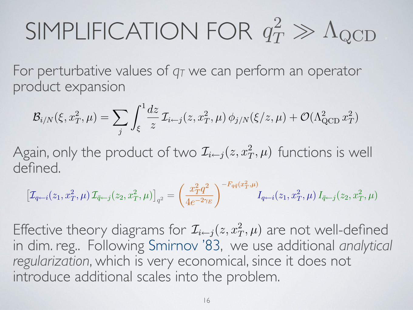
SIMPLIFICATION FOR .

For perturbative values of qT we can perform an operator product expansion

Again, only the product of two functions is well defined.

Effective theory diagrams for are not well-defined in dim. reg.. Following Smirnov ’83, we use additional analytical regularization, which is very economical, since it does not introduce additional scales into the problem.

〈N1(p)| χhc(x+ + x⊥)/n χhc(0) |N1(p)〉

Aµs (x) = Aµ

s (0) + x · ∂Aµs (0) + . . .

φq/N(z, µ) =1

2π

∫


2χ(0) |N(p)〉

Bq/N (z, x2T , µ) =

1

2π

∫


2χ(0) |N(p)〉

(9)

d3σ

dM2 dq2T dy

=4πα2

3NcM2s

∣

∣CV (−M2, µ)∣

∣

2 1

4π

∫


×∑

q

e2q

[

Bq/N1(ξ1, x

2T , µ)Bq/N2

(ξ2, x2T , µ) + (q ↔ q)

]

+ O(

q2T

M2

)

,

(10)

d3σ

dM2 dq2T dy

=4πα2

3NcM2s

∣

∣CV (−M2, µ)∣

∣

2 1

4π

∫


(

x2T M2

4e−2γE

)−Fqq(x2

T ,µ)

×∑

q

e2q

[

Bq/N1(ξ1, x

2T , µ)Bq/N2

(ξ2, x2T , µ) + (q ↔ q)

]

+ O(

q2T

M2

)

,

(11)

where

ξ1 =√

τ ey , ξ2 =√


⊥

s=

M2 + q2T

s. (12)

[

Bq/N1(z1, x

2T , µ)Bq/N2

(z2, x2T , µ)

]

q2=

(

x2T q2

4e−2γE

)−Fqq(x2

T ,µ)

Bq/N1(z1, x

2T , µ)Bq/N2

(z2, x2T , µ) ,

dFqq(x2T , µ)

d lnµ= 2ΓF

cusp(αs) (13)

d

d lnµCV (M2, µ) =

[

ΓFcusp(αs) ln

−M2

µ2+ 2γq(αs)

]

CV (M2, µ) . (14)

q2T ' ΛQCD (15)

2

It will also be useful to study the total cross section defined with a cut qT ≤ QT , which vetoessingle jet emission. Neglecting the dependence of the variable τ in (17) on q2

T , which is apower-suppressed effect, we obtain from (24)

dσ

dM2

∣

∣

∣

∣

qT ≤QT

=4πα2

3NcM2s

∑

q

e2q

∑

i=q,g

∑

j=q,g

∫∫

z1z2≥M2/s

dz1

z1

dz2

z2(26)

×[

min(Q2T , z1z2s−M2)∫

0

dq2T Cqq→ij(z1, z2, q

2T , M2, µ) ffij

( M2

z1z2s, µ

)

+ (q, i ↔ q, j)

]

.

3 Calculation of the kernels Iq←q and Iq←g

We now perform a perturbative calculation of the relevant kernels Ii←j entering the factor-ization formula (22) at first non-trivial order in αs. Since we do not have explicit operatordefinitions of the (good) transverse distribution functions Bi/N , we analyze instead the original(bad) functions Bi/N defined in (11), keeping in mind that only products of two such functionsreferring to different hadrons are well defined. If we write an operator-product expansionanalogous to (19)

Bi/N (ξ, x2T , µ) =

∑

j

∫ 1

ξ

dz

zIi←j(z, x

2T , µ) φj/N(ξ/z, µ) + O(Λ2

QCD x2T ) , (27)

it follows that the products of two Ii←j functions are well defined and obey a factorizationformula analogous to (13).

3.1 One-loop results

Perturbative expansions for the kernels Ii←j can be derived from a matching calculation, inwhich the matrix elements in (10) and (11) are evaluated using external parton states carryinga fixed fraction of the nucleon momentum p. The tree-level result is obviously given by

Ii←j(z, x2T , µ) = δ(1 − z) δij + O(αs) . (28)

The relevant one-loop diagrams giving rise to the O(αs) corrections to the kernels Iq←q = Iq←q

are shown in the first row of Figure 1. There is no need to consider diagrams with external-legcorrections on only one side of the cut, because these give identical contributions to Bi/N andφi/N and thus do not change the tree-level result (28). Working in Feynman gauge, we findthat the contribution of the first diagram is

Iaq←q(z, x

2T , µ) = −

CF αs

2π(1 − z)

(

1

ε+ L⊥ − 1

)

, L⊥ = lnx2

T µ2

4e−2γE, (29)

while the fourth diagram gives a vanishing result, Idq←q = 0. As before, αs ≡ αs(µ) always

10



dσ

dM2

∣

∣

∣

∣

qT ≤QT

=4πα2

3NcM2s

∑

q

e2q

∑

i=q,g

∑

j=q,g

∫∫

z1z2≥M2/s

dz1

z1

dz2

z2(26)

×[


0


2T , M2, µ) ffij

( M2

z1z2s, µ

)

+ (q, i ↔ q, j)

]

.



Bi/N (ξ, x2T , µ) =

∑

j

∫ 1

ξ

dz

zIi←j(z, x

2T , µ) φj/N(ξ/z, µ) + O(Λ2

QCD x2T ) , (27)







Iaq←q(z, x

2T , µ) = −

CF αs

2π(1 − z)

(

1

ε+ L⊥ − 1

)

, L⊥ = lnx2

T µ2

4e−2γE, (29)


10



dσ

dM2

∣

∣

∣

∣

qT ≤QT

=4πα2

3NcM2s

∑

q

e2q

∑

i=q,g

∑

j=q,g

∫∫

z1z2≥M2/s

dz1

z1

dz2

z2(26)

×[


0


2T , M2, µ) ffij

( M2

z1z2s, µ

)

+ (q, i ↔ q, j)

]

.



Bi/N (ξ, x2T , µ) =

∑

j

∫ 1

ξ

dz

zIi←j(z, x

2T , µ) φj/N(ξ/z, µ) + O(Λ2

QCD x2T ) , (27)







Iaq←q(z, x

2T , µ) = −

CF αs

2π(1 − z)

(

1

ε+ L⊥ − 1

)

, L⊥ = lnx2

T µ2

4e−2γE, (29)


10

〈N1(p)| χhc(x+ + x⊥)/n χhc(0) |N1(p)〉

Aµs (x) = Aµ

s (0) + x · ∂Aµs (0) + . . .

φq/N(z, µ) =1

2π

∫


2χ(0) |N(p)〉

Bq/N (z, x2T , µ) =

1

2π

∫


2χ(0) |N(p)〉

(9)

d3σ

dM2 dq2T dy

=4πα2

3NcM2s

∣

∣CV (−M2, µ)∣

∣

2 1

4π

∫


×∑

q

e2q

[

Bq/N1(ξ1, x

2T , µ)Bq/N2

(ξ2, x2T , µ) + (q ↔ q)

]

+ O(

q2T

M2

)

,

(10)

d3σ

dM2 dq2T dy

=4πα2

3NcM2s

∣

∣CV (−M2, µ)∣

∣

2 1

4π

∫


(

x2T M2

4e−2γE

)−Fqq(x2

T ,µ)

×∑

q

e2q

[

Bq/N1(ξ1, x

2T , µ)Bq/N2

(ξ2, x2T , µ) + (q ↔ q)

]

+ O(

q2T

M2

)

,

(11)

where

ξ1 =√

τ ey , ξ2 =√


⊥

s=

M2 + q2T

s. (12)

[

Bq/N1(z1, x

2T , µ)Bq/N2

(z2, x2T , µ)

]

q2=

(

x2T q2

4e−2γE

)−Fqq(x2

T ,µ)

Bq/N1(z1, x

2T , µ)Bq/N2

(z2, x2T , µ) ,

dFqq(x2T , µ)

d lnµ= 2ΓF

cusp(αs) (13)

d

d lnµCV (M2, µ) =

[

ΓFcusp(αs) ln

−M2

µ2+ 2γq(αs)

]

CV (M2, µ) . (14)

q2T ' ΛQCD (15)


[


2T , µ)

]

q2=

(

x2T q2

4e−2γE

)−Fqq(x2

T ,µ)


2T , µ) ,

2

16

ANALYTICAL REGULARIZATION

• Raise QCD propagators carrying large momentum to fractional powers :

• Limit is trivial for QCD, but effective theory diagrams have poles, which only cancel in the sum of collinear and anti-collinear diagrams.

hc hc

hc hc

βα → xx

xx

hc hc

hc

hc

hc

β α +xx

xx

hchc

hc

hc hc

βα

Figure 2: Matching of an analytically-regularized QCD graph onto SCET diagrams.

of diagrams develop singularities in the limit β → 0 followed by α → 0 or vice versa, whichcancel in the sum of the results from both sectors.

With the analytic regulators in place, the remaining two diagrams in Figure 1 can now becomputed and both give the same result. For their sum, we obtain

Ib+cq←q(z, x

2T , µ) =

CFαs

2πeεγE

(

µ2

ν21

)−α (

q2

ν22

)−β 2z

(1 − z)1−α+β

Γ(−ε − α)

Γ(1 + α)

(

x2T µ2

4

)ε+α

. (32)

Like in full QCD, the analytic regulators must be taken to zero before taking the limit ε → 0.The result depends on the order in which the limits α → 0 and β → 0 are performed. Ex-panding first in β and then in α, the light-cone singularities are regulated by the α parameter,and we find for the sum of all four one-loop diagrams

Iq←q(z, x2T , µ)

∣

∣

∣

α reg.= −

CFαs

2π

{(

1

ε+ L⊥

) [(

2

α− 2 ln

µ2

ν21

)

δ(1 − z) +1 + z2

(1 − z)+

]

+ δ(1 − z)

(

−2

ε2+ L2

⊥ +π2

6

)

− (1 − z)

}

. (33)

If the expansions are performed in the opposite order, then β acts as the analytic regulator,and we obtain

Iq←q(z, x2T , µ)

∣

∣

∣

β reg.= −

CF αs

2π

{(

1

ε+ L⊥

) [(

−2

β+ 2 ln

q2

ν22

)

δ(1 − z) +1 + z2

(1 − z)+

]

−(1−z)

}

.

(34)The above results refer to the kernel associated with hard-collinear partons, which propa-

gate along the n direction. Let us now consider what happens when we calculate the corre-sponding kernel for anti-hard-collinear fields. In that case we get the same answer but withα, ν1 and β, ν2 interchanged. We then find that in the product of a hard-collinear and ananti-hard-collinear kernel function the analytic regulators disappear, no matter in which orderthe limits α → 0 and β → 0 are taken. This product is thus regulator independent and welldefined in dimensional regularization. After MS subtractions, we obtain

[

Iq←q(z1, x2T , µ) Iq←q(z2, x

2T , µ)

]

q2

= δ(1 − z1) δ(1 − z2)

[

1 −CFαs

2π

(

2L⊥ lnq2

µ2+ L2

⊥ − 3L⊥ +π2

6

)]

−CF αs

2π

{

δ(1 − z1)

[

L⊥

(

1 + z22

1 − z2

)

+

− (1 − z2)

]

+ (z1 ↔ z2)

}

+ O(α2s) .

(35)

12

xx xx xx xx

xx

Figure 1: One-loop diagrams contributing to the matching coefficients Iq←q (top row) andIq←g (bottom row). The vertical lines indicate cut propagators.

refers to the running coupling evaluated at the scale µ, unless indicated otherwise. Thedimensional regulator is defined by d = 4− 2ε, and we omit O(ε) terms. Moreover, µ denotesthe renormalization scale defined in the MS scheme. The remaining two diagrams turn outto be ill-defined in dimensional regularization due to light-cone singularities. To give meaningto the corresponding loop integrals requires introducing additional regulators. The simplestpossibility is to employ analytic regularization, as is common in the context of asymptoticexpansions [19, 20]. In the context of SCET this method has been used in [15, 44]. One startsby reconsidering the QCD diagrams contributing to the process and raises all propagatorsthrough which the external hard-collinear momentum p flows to a fractional power,

1

−(p − k)2 − iε→

ν2α1

[−(p − k)2 − iε]1+α , (30)

and similarly for the anti-hard-collinear propagators, but with a different regulator β andassociated scale ν2. For QCD diagrams, such as the first graph in Figure 2, the modificationis trivial in the sense that the limits α → 0 and β → 0 are smooth as long as ε is kept finite.However, with the analytic regulators in place also the SCET diagrams in the (anti-)hard-collinear sectors are now also well-defined. The diagrams in each sector involve divergencesin the analytical regulator, which cancel in the sum of all contributions. If the momentumk in (30) is hard-collinear, as in the first SCET diagram in Figure 2, the regularization inthe effective theory takes the same form as in QCD. If, on the other hand, the momentumk is anti-hard-collinear, then the propagator is far off-shell and in SCET is represented by aWilson line, as shown in the second diagram in Figure 2. Using the replacement rule (30) andperforming the appropriate expansions, we find that the Feynman rule for a gluon emissionfrom the anti-hard-collinear Wilson line Whc in the current operator (6) gets replaced by

nµ

n · k − iε→

ν2α1 nµ n · p

(n · k n · p − iε)1+α . (31)

As seen in Figure 2, the regulator α plays a double role: it regularizes the fermion propagatorsin hard-collinear diagrams and the Wilson lines in anti-hard-collinear diagrams. Both classes

11

〈N1(p)| χhc(x+ + x⊥)/n χhc(0) |N1(p)〉

Aµs (x) = Aµ

s (0) + x · ∂Aµs (0) + . . .

φq/N(z, µ) =1

2π

∫


2χ(0) |N(p)〉

Bq/N (z, x2T , µ) =

1

2π

∫


2χ(0) |N(p)〉

(9)

d3σ

dM2 dq2T dy

=4πα2

3NcM2s

∣

∣CV (−M2, µ)∣

∣

2 1

4π

∫


×∑

q

e2q

[

Bq/N1(ξ1, x

2T , µ)Bq/N2

(ξ2, x2T , µ) + (q ↔ q)

]

+ O(

q2T

M2

)

,

(10)

d3σ

dM2 dq2T dy

=4πα2

3NcM2s

∣

∣CV (−M2, µ)∣

∣

2 1

4π

∫


(

x2T M2

4e−2γE

)−Fqq(x2

T ,µ)

×∑

q

e2q

[

Bq/N1(ξ1, x

2T , µ)Bq/N2

(ξ2, x2T , µ) + (q ↔ q)

]

+ O(

q2T

M2

)

,

(11)

where

ξ1 =√

τ ey , ξ2 =√


⊥

s=

M2 + q2T

s. (12)

[

Bq/N1(z1, x

2T , µ)Bq/N2

(z2, x2T , µ)

]

q2=

(

x2T q2

4e−2γE

)−Fqq(x2

T ,µ)

Bq/N1(z1, x

2T , µ)Bq/N2

(z2, x2T , µ) ,

dFqq(x2T , µ)

d lnµ= 2ΓF

cusp(αs) (13)

d

d lnµCV (M2, µ) =

[

ΓFcusp(αs) ln

−M2

µ2+ 2γq(αs)

]

CV (M2, µ) . (14)

q2T ' ΛQCD (15)

Text p, (p) to the power α, (β)

2

〈N1(p)| χhc(x+ + x⊥)/n χhc(0) |N1(p)〉

Aµs (x) = Aµ

s (0) + x · ∂Aµs (0) + . . .

φq/N(z, µ) =1

2π

∫


2χ(0) |N(p)〉

Bq/N (z, x2T , µ) =

1

2π

∫


2χ(0) |N(p)〉

(9)

d3σ

dM2 dq2T dy

=4πα2

3NcM2s

∣

∣CV (−M2, µ)∣

∣

2 1

4π

∫


×∑

q

e2q

[

Bq/N1(ξ1, x

2T , µ)Bq/N2

(ξ2, x2T , µ) + (q ↔ q)

]

+ O(

q2T

M2

)

,

(10)

d3σ

dM2 dq2T dy

=4πα2

3NcM2s

∣

∣CV (−M2, µ)∣

∣

2 1

4π

∫


(

x2T M2

4e−2γE

)−Fqq(x2

T ,µ)

×∑

q

e2q

[

Bq/N1(ξ1, x

2T , µ)Bq/N2

(ξ2, x2T , µ) + (q ↔ q)

]

+ O(

q2T

M2

)

,

(11)

where

ξ1 =√

τ ey , ξ2 =√


⊥

s=

M2 + q2T

s. (12)

[

Bq/N1(z1, x

2T , µ)Bq/N2

(z2, x2T , µ)

]

q2=

(

x2T q2

4e−2γE

)−Fqq(x2

T ,µ)

Bq/N1(z1, x

2T , µ)Bq/N2

(z2, x2T , µ) ,

dFqq(x2T , µ)

d lnµ= 2ΓF

cusp(αs) (13)

d

d lnµCV (M2, µ) =

[

ΓFcusp(αs) ln

−M2

µ2+ 2γq(αs)

]

CV (M2, µ) . (14)

q2T ' ΛQCD (15)

Text p, (p) to the power α, (β)

2

〈N1(p)| χhc(x+ + x⊥)/n χhc(0) |N1(p)〉

Aµs (x) = Aµ

s (0) + x · ∂Aµs (0) + . . .

φq/N(z, µ) =1

2π

∫


2χ(0) |N(p)〉

Bq/N (z, x2T , µ) =

1

2π

∫


2χ(0) |N(p)〉

(9)

d3σ

dM2 dq2T dy

=4πα2

3NcM2s

∣

∣CV (−M2, µ)∣

∣

2 1

4π

∫


×∑

q

e2q

[

Bq/N1(ξ1, x

2T , µ)Bq/N2

(ξ2, x2T , µ) + (q ↔ q)

]

+ O(

q2T

M2

)

,

(10)

d3σ

dM2 dq2T dy

=4πα2

3NcM2s

∣

∣CV (−M2, µ)∣

∣

2 1

4π

∫


(

x2T M2

4e−2γE

)−Fqq(x2

T ,µ)

×∑

q

e2q

[

Bq/N1(ξ1, x

2T , µ)Bq/N2

(ξ2, x2T , µ) + (q ↔ q)

]

+ O(

q2T

M2

)

,

(11)

where

ξ1 =√

τ ey , ξ2 =√


⊥

s=

M2 + q2T

s. (12)

[

Bq/N1(z1, x

2T , µ)Bq/N2

(z2, x2T , µ)

]

q2=

(

x2T q2

4e−2γE

)−Fqq(x2

T ,µ)

Bq/N1(z1, x

2T , µ)Bq/N2

(z2, x2T , µ) ,

dFqq(x2T , µ)

d lnµ= 2ΓF

cusp(αs) (13)

d

d lnµCV (M2, µ) =

[

ΓFcusp(αs) ln

−M2

µ2+ 2γq(αs)

]

CV (M2, µ) . (14)

q2T ' ΛQCD (15)

Text p, (p) to the power α → 0, β → 0

2

17

ANALYTICAL REGULARIZATION

• Regulators play double role. E.g. regulates hc propagators and hc Wilson line

• Regulator breaks invariance of anti-hard-collinear sector under a rescaling of the hard-collinear momentum .

hc hc

hc hc

βα → xx

xx

hc hc

hc

hc

hc

β α +xx

xx

hchc

hc

hc hc

βα

Figure 2: Matching of an analytically-regularized QCD graph onto SCET diagrams.

of diagrams develop singularities in the limit β → 0 followed by α → 0 or vice versa, whichcancel in the sum of the results from both sectors.


Ib+cq←q(z, x

2T , µ) =

CFαs

2πeεγE

(

µ2

ν21

)−α (

q2

ν22

)−β 2z

(1 − z)1−α+β

Γ(−ε − α)

Γ(1 + α)

(

x2T µ2

4

)ε+α

. (32)


Iq←q(z, x2T , µ)

∣

∣

∣

α reg.= −

CFαs

2π

{(

1

ε+ L⊥

) [(

2

α− 2 ln

µ2

ν21

)

δ(1 − z) +1 + z2

(1 − z)+

]

+ δ(1 − z)

(

−2

ε2+ L2

⊥ +π2

6

)

− (1 − z)

}

. (33)


Iq←q(z, x2T , µ)

∣

∣

∣

β reg.= −

CF αs

2π

{(

1

ε+ L⊥

) [(

−2

β+ 2 ln

q2

ν22

)

δ(1 − z) +1 + z2

(1 − z)+

]

−(1−z)

}

.

(34)The above results refer to the kernel associated with hard-collinear partons, which propa-

gate along the n direction. Let us now consider what happens when we calculate the corre-sponding kernel for anti-hard-collinear fields. In that case we get the same answer but withα, ν1 and β, ν2 interchanged. We then find that in the product of a hard-collinear and ananti-hard-collinear kernel function the analytic regulators disappear, no matter in which orderthe limits α → 0 and β → 0 are taken. This product is thus regulator independent and welldefined in dimensional regularization. After MS subtractions, we obtain

[

Iq←q(z1, x2T , µ) Iq←q(z2, x

2T , µ)

]

q2

= δ(1 − z1) δ(1 − z2)

[

1 −CFαs

2π

(

2L⊥ lnq2

µ2+ L2

⊥ − 3L⊥ +π2

6

)]

−CF αs

2π

{

δ(1 − z1)

[

L⊥

(

1 + z22

1 − z2

)

+

− (1 − z2)

]

+ (z1 ↔ z2)

}

+ O(α2s) .

(35)

12

is trivial in the sense that the limits α → 0 and β → 0 are smooth as long as ε is kept finite.However, with the analytic regulators in place the contributions of the different momentumregions are now well-defined individually and one can check which regions give non-vanishingcontributions to the expansion of the integral. One finds that only the hard, the hard-collinearand anti-hard-collinear regions contribute. If the diagrams are evaluated off-shell, then also asoft contribution arises in the individual diagrams, but one easily verifies that the contributionof a semi-hard mode scaling as M(λ, λ, λ) vanishes.

Since the original diagram is well defined without the analytical regulators and is obtainedby adding up the contributions from the different regions, we are guaranteed that the limitsα → 0 and β → 0 can be taken in the sum and that the result is independent of the regula-tor. Individually, however, the diagrams in each sector involve divergences in the analyticalregulators. If the momentum k in (31) is hard-collinear, as in the first SCET diagram inFigure 2, the regularization in the effective theory takes the same form as in QCD. If, on theother hand, the momentum k is anti-hard-collinear, then the propagator is far off-shell and inSCET is represented by a Wilson line, as shown in the second diagram in Figure 2. Using thereplacement rule (31) and performing the appropriate expansions, we find that the Feynmanrule for a gluon emission from the anti-hard-collinear Wilson line Whc in the current operator(6) gets replaced by

nµ

n · k − iε→

ν2α1 nµ n · p

(n · k n · p − iε)1+α . (32)

Note that, as mentioned earlier in Section 2.2, the regularized Feynman rule for the anti-hard-collinear Wilson line is no longer invariant under the rescaling transformation p → λp. Asseen in Figure 2, the regulator α plays a double role: it regularizes the fermion propagatorsin hard-collinear diagrams and the Wilson lines in anti-hard-collinear diagrams. Both classesof diagrams develop singularities in the limit β → 0 followed by α → 0 or vice versa, whichcancel in the sum of the results from both sectors.


Ib+cq←q(z, x

2T , µ) =

CFαs

2πeεγE

(

µ2

ν21

)−α (

q2

ν22

)−β 2z

(1 − z)1−α+β

Γ(−ε − α)

Γ(1 + α)

(

x2T µ2

4

)ε+α

. (33)


Iq←q(z, x2T , µ)

∣

∣

∣

α reg.= −

CFαs

2π

{(

1

ε+ L⊥

) [(

2

α− 2 ln

µ2

ν21

)

δ(1 − z) +1 + z2

(1 − z)+

]

+ δ(1 − z)

(

−2

ε2+ L2

⊥ +π2

6

)

− (1 − z)

}

. (34)

If the expansions are performed in the opposite order, then β acts as the analytic regulator,

12

〈N1(p)| χhc(x+ + x⊥)/n χhc(0) |N1(p)〉

Aµs (x) = Aµ

s (0) + x · ∂Aµs (0) + . . .

φq/N(z, µ) =1

2π

∫


2χ(0) |N(p)〉

Bq/N (z, x2T , µ) =

1

2π

∫


2χ(0) |N(p)〉

(9)

d3σ

dM2 dq2T dy

=4πα2

3NcM2s

∣

∣CV (−M2, µ)∣

∣

2 1

4π

∫


×∑

q

e2q

[

Bq/N1(ξ1, x

2T , µ)Bq/N2

(ξ2, x2T , µ) + (q ↔ q)

]

+ O(

q2T

M2

)

,

(10)

d3σ

dM2 dq2T dy

=4πα2

3NcM2s

∣

∣CV (−M2, µ)∣

∣

2 1

4π

∫


(

x2T M2

4e−2γE

)−Fqq(x2

T ,µ)

×∑

q

e2q

[

Bq/N1(ξ1, x

2T , µ)Bq/N2

(ξ2, x2T , µ) + (q ↔ q)

]

+ O(

q2T

M2

)

,

(11)

where

ξ1 =√

τ ey , ξ2 =√


⊥

s=

M2 + q2T

s. (12)

[

Bq/N1(z1, x

2T , µ)Bq/N2

(z2, x2T , µ)

]

q2=

(

x2T q2

4e−2γE

)−Fqq(x2

T ,µ)

Bq/N1(z1, x

2T , µ)Bq/N2

(z2, x2T , µ) ,

dFqq(x2T , µ)

d lnµ= 2ΓF

cusp(αs) (13)

d

d lnµCV (M2, µ) =

[

ΓFcusp(αs) ln

−M2

µ2+ 2γq(αs)

]

CV (M2, µ) . (14)

q2T ' ΛQCD (15)

Text p, (p) to the power α → 0, β → 0

2

〈N1(p)| χhc(x+ + x⊥)/n χhc(0) |N1(p)〉

Aµs (x) = Aµ

s (0) + x · ∂Aµs (0) + . . .

φq/N(z, µ) =1

2π

∫


2χ(0) |N(p)〉

Bq/N (z, x2T , µ) =

1

2π

∫


2χ(0) |N(p)〉

(9)

d3σ

dM2 dq2T dy

=4πα2

3NcM2s

∣

∣CV (−M2, µ)∣

∣

2 1

4π

∫


×∑

q

e2q

[

Bq/N1(ξ1, x

2T , µ)Bq/N2

(ξ2, x2T , µ) + (q ↔ q)

]

+ O(

q2T

M2

)

,

(10)

d3σ

dM2 dq2T dy

=4πα2

3NcM2s

∣

∣CV (−M2, µ)∣

∣

2 1

4π

∫


(

x2T M2

4e−2γE

)−Fqq(x2

T ,µ)

×∑

q

e2q

[

Bq/N1(ξ1, x

2T , µ)Bq/N2

(ξ2, x2T , µ) + (q ↔ q)

]

+ O(

q2T

M2

)

,

(11)

where

ξ1 =√

τ ey , ξ2 =√


⊥

s=

M2 + q2T

s. (12)

[

Bq/N1(z1, x

2T , µ)Bq/N2

(z2, x2T , µ)

]

q2=

(

x2T q2

4e−2γE

)−Fqq(x2

T ,µ)

Bq/N1(z1, x

2T , µ)Bq/N2

(z2, x2T , µ) ,

dFqq(x2T , µ)

d lnµ= 2ΓF

cusp(αs) (13)

d

d lnµCV (M2, µ) =

[

ΓFcusp(αs) ln

−M2

µ2+ 2γq(αs)

]

CV (M2, µ) . (14)

q2T ' ΛQCD (15)


2

18

1-LOOP RESULTTaking first , then , one finds ( )

In the product the divergences vanish, but anomalous M2 dependence remains.

Iq←q(z, x2T , µ) = δ(1 − z) −

CFαs

2π

{(

1

ε+ L⊥

) [(

2

α− 2 ln

µ2

ν21

)

δ(1 − z) +1 + z2

(1 − z)+

]

+ δ(1 − z)

(

−2

ε2+ L2

⊥ +π2

6

)

− (1 − z)

}

(16)


Iq←q(z, x2T , µ) = δ(1 − z) −

CF αs

2π

{(

1

ε+ L⊥

) [(

−2

α+ 2 ln

q2

ν21

)

δ(1 − z)

+1 + z2

(1 − z)+

]

− (1 − z)

}

(17)

3

Iq←q(z, x2T , µ) = δ(1 − z) −

CFαs

2π

{(

1

ε+ L⊥

) [(

2

α− 2 ln

µ2

ν21

)

δ(1 − z) +1 + z2

(1 − z)+

]

+ δ(1 − z)

(

−2

ε2+ L2

⊥ +π2

6

)

− (1 − z)

}

(16)


Iq←q(z, x2T , µ) = δ(1 − z) −

CFαs

2π

{(

1

ε+ L⊥

) [(

−2

α+ 2 ln

M2

ν21

)

δ(1 − z)

+1 + z2

(1 − z)+

]

− (1 − z)

}

(17)

3

〈N1(p)| χhc(x+ + x⊥)/n χhc(0) |N1(p)〉

Aµs (x) = Aµ

s (0) + x · ∂Aµs (0) + . . .

φq/N(z, µ) =1

2π

∫


2χ(0) |N(p)〉

Bq/N (z, x2T , µ) =

1

2π

∫


2χ(0) |N(p)〉

(9)

d3σ

dM2 dq2T dy

=4πα2

3NcM2s

∣

∣CV (−M2, µ)∣

∣

2 1

4π

∫


×∑

q

e2q

[

Bq/N1(ξ1, x

2T , µ)Bq/N2

(ξ2, x2T , µ) + (q ↔ q)

]

+ O(

q2T

M2

)

,

(10)

d3σ

dM2 dq2T dy

=4πα2

3NcM2s

∣

∣CV (−M2, µ)∣

∣

2 1

4π

∫


(

x2T M2

4e−2γE

)−Fqq(x2

T ,µ)

×∑

q

e2q

[

Bq/N1(ξ1, x

2T , µ)Bq/N2

(ξ2, x2T , µ) + (q ↔ q)

]

+ O(

q2T

M2

)

,

(11)

where

ξ1 =√

τ ey , ξ2 =√


⊥

s=

M2 + q2T

s. (12)

[

Bq/N1(z1, x

2T , µ)Bq/N2

(z2, x2T , µ)

]

q2=

(

x2T q2

4e−2γE

)−Fqq(x2

T ,µ)

Bq/N1(z1, x

2T , µ)Bq/N2

(z2, x2T , µ) ,

dFqq(x2T , µ)

d lnµ= 2ΓF

cusp(αs) (13)

d

d lnµCV (M2, µ) =

[

ΓFcusp(αs) ln

−M2

µ2+ 2γq(αs)

]

CV (M2, µ) . (14)

q2T ' ΛQCD (15)


[


2T , µ)

]

q2=

(

x2T q2

4e−2γE

)−Fqq(x2

T ,µ)


2T , µ) ,

2

〈N1(p)| χhc(x+ + x⊥)/n χhc(0) |N1(p)〉

Aµs (x) = Aµ

s (0) + x · ∂Aµs (0) + . . .

φq/N(z, µ) =1

2π

∫


2χ(0) |N(p)〉

Bq/N (z, x2T , µ) =

1

2π

∫


2χ(0) |N(p)〉

(9)

d3σ

dM2 dq2T dy

=4πα2

3NcM2s

∣

∣CV (−M2, µ)∣

∣

2 1

4π

∫


×∑

q

e2q

[

Bq/N1(ξ1, x

2T , µ)Bq/N2

(ξ2, x2T , µ) + (q ↔ q)

]

+ O(

q2T

M2

)

,

(10)

d3σ

dM2 dq2T dy

=4πα2

3NcM2s

∣

∣CV (−M2, µ)∣

∣

2 1

4π

∫


(

x2T M2

4e−2γE

)−Fqq(x2

T ,µ)

×∑

q

e2q

[

Bq/N1(ξ1, x

2T , µ)Bq/N2

(ξ2, x2T , µ) + (q ↔ q)

]

+ O(

q2T

M2

)

,

(11)

where

ξ1 =√

τ ey , ξ2 =√


⊥

s=

M2 + q2T

s. (12)

[

Bq/N1(z1, x

2T , µ)Bq/N2

(z2, x2T , µ)

]

q2=

(

x2T q2

4e−2γE

)−Fqq(x2

T ,µ)

Bq/N1(z1, x

2T , µ)Bq/N2

(z2, x2T , µ) ,

dFqq(x2T , µ)

d lnµ= 2ΓF

cusp(αs) (13)

d

d lnµCV (M2, µ) =

[

ΓFcusp(αs) ln

−M2

µ2+ 2γq(αs)

]

CV (M2, µ) . (14)

q2T ' ΛQCD (15)


[


2T , µ)

]

q2=

(

x2T q2

4e−2γE

)−Fqq(x2

T ,µ)


2T , µ) ,

2

Iq←q(z, x2T , µ) = δ(1 − z) −

CFαs

2π

{(

1

ε+ L⊥

) [(

2

α− 2 ln

µ2

ν21

)

δ(1 − z) +1 + z2

(1 − z)+

]

+ δ(1 − z)

(

−2

ε2+ L2

⊥ +π2

6

)

− (1 − z)

}

(16)


Iq←q(z, x2T , µ) = δ(1 − z) −

CFαs

2π

{(

1

ε+ L⊥

) [(

−2

α+ 2 ln

M2

ν21

)

δ(1 − z)

+1 + z2

(1 − z)+

]

− (1 − z)

}

(17)

1/α

3

anomalous M2 dep.

19

×[

Cqi

(

z1, αs(µb))

Cqj

(

z2, αs(µb))

φi/N1(ξ1/z1, µb) φj/N2

(ξ2/z2, µb) + (q, i ↔ q, j)

]

,

µb = b0/xT , and we adopt the standard choice b0 = 2e−γE

L⊥ = lnx2

T µ2

4e−2γE

5

• For the functions I and F, one then obtains

• Solving its RG and using Davies, Stirling and Webber ’84 and de Florian and Grazzini ’01, we extract the two-loop F

Iq←q(z, x2T , µ) = δ(1 − z) −

CFαs

2π

{(

1

ε+ L⊥

) [(

2

α− 2 ln

µ2

ν21

)

δ(1 − z) +1 + z2

(1 − z)+

]

+ δ(1 − z)

(

−2

ε2+ L2

⊥ +π2

6

)

− (1 − z)

}

(16)


Iq←q(z, x2T , µ) = δ(1 − z) −

CFαs

2π

{(

1

ε+ L⊥

) [(

−2

α+ 2 ln

M2

ν21

)

δ(1 − z)

+1 + z2

(1 − z)+

]

− (1 − z)

}

(17)

1/α

Fqq(L⊥, αs) =CFαs

πL⊥ + O(α2

s)

Iq←q(z, L⊥, αs) = Iq←q(z, L⊥, αs) = δ(1 − z)

[

1 +CFαs

4π

(

L2⊥ + 3L⊥ −

π2

6

)]

−CFαs

2π

[

L⊥Pq←q(z) − (1 − z)]

+ O(α2s)

Iq←g(z, L⊥, αs) = Iq←g(z, L⊥, αs) = −TF αs

2π

[

L⊥Pq←g(z) − 2z(1 − z)]

+ O(α2s)

(18)

3

Iq←q(z, x2T , µ) = δ(1 − z) −

CFαs

2π

{(

1

ε+ L⊥

) [(

2

α− 2 ln

µ2

ν21

)

δ(1 − z) +1 + z2

(1 − z)+

]

+ δ(1 − z)

(

−2

ε2+ L2

⊥ +π2

6

)

− (1 − z)

}

(16)


Iq←q(z, x2T , µ) = δ(1 − z) −

CFαs

2π

{(

1

ε+ L⊥

) [(

−2

α+ 2 ln

M2

ν21

)

δ(1 − z)

+1 + z2

(1 − z)+

]

− (1 − z)

}

(17)

1/α


πL⊥ + O(α2

s)


[

1 +CFαs

4π

(

L2⊥ + 3L⊥ −

π2

6

)]

−CFαs

2π

[

L⊥Pq←q(z) − (1 − z)]

+ O(α2s)


2π

[

L⊥Pq←g(z) − 2z(1 − z)]

+ O(α2s)

(18)

For the first two expansion coefficients, we obtain

Fqq(L⊥, αs) =αs

4πΓF

0 L⊥ +(αs

4π

)2[

ΓF0 β0

2L2⊥ + ΓF

1 L⊥ + dq2

]

(19)

dq2 = CF

[

CA

(

808

27− 28ζ3

)

−224

27TF nf

]

(20)

Fqq(L⊥, αs)

CF=

Fgg(L⊥, αs)

CA(21)

3

Casimir scaling

Iq←q(z, x2T , µ) = δ(1 − z) −

CFαs

2π

{(

1

ε+ L⊥

) [(

2

α− 2 ln

µ2

ν21

)

δ(1 − z) +1 + z2

(1 − z)+

]

+ δ(1 − z)

(

−2

ε2+ L2

⊥ +π2

6

)

− (1 − z)

}

(16)


Iq←q(z, x2T , µ) = δ(1 − z) −

CFαs

2π

{(

1

ε+ L⊥

) [(

−2

α+ 2 ln

M2

ν21

)

δ(1 − z)

+1 + z2

(1 − z)+

]

− (1 − z)

}

(17)

1/α


πL⊥ + O(α2

s)


[

1 +CFαs

4π

(

L2⊥ + 3L⊥ −

π2

6

)]

−CFαs

2π

[

L⊥Pq←q(z) − (1 − z)]

+ O(α2s)


2π

[

L⊥Pq←g(z) − 2z(1 − z)]

+ O(α2s)

(18)


Fqq(L⊥, αs) =αs

4πΓF

0 L⊥ +(αs

4π

)2[

ΓF0 β0

2L2⊥ + ΓF

1 L⊥ + dq2

]

(19)

dq2 = CF

[

CA

(

808

27− 28ζ3

)

−224

27TF nf

]

(20)

Fqq(L⊥, αs)

CF=

Fgg(L⊥, αs)

CA(21)

3

All the necessary input for NNLL resummation!20

RESUMMED RESULT

The hard-scattering kernel is

• Two sources of M dependence: hard function and anomaly

• Fourier transform can be evaluated numerically or analytically, if higher-log terms are expanded out.

Cqq→ij(z1, z2, q2T , M2, µ) =

∣

∣CV (−M2, µ)∣

∣

2 1

4π

∫


(

x2T M2

4e−2γE

)−Fqq(x2

T ,µ)


2T , µ)

(23)

4

Iq←q(z, x2T , µ) = δ(1 − z) −

CFαs

2π

{(

1

ε+ L⊥

) [(

2

α− 2 ln

µ2

ν21

)

δ(1 − z) +1 + z2

(1 − z)+

]

+ δ(1 − z)

(

−2

ε2+ L2

⊥ +π2

6

)

− (1 − z)

}

(16)


Iq←q(z, x2T , µ) = δ(1 − z) −

CFαs

2π

{(

1

ε+ L⊥

) [(

−2

α+ 2 ln

M2

ν21

)

δ(1 − z)

+1 + z2

(1 − z)+

]

− (1 − z)

}

(17)

1/α


πL⊥ + O(α2

s)


[

1 +CFαs

4π

(

L2⊥ + 3L⊥ −

π2

6

)]

−CFαs

2π

[

L⊥Pq←q(z) − (1 − z)]

+ O(α2s)


2π

[

L⊥Pq←g(z) − 2z(1 − z)]

+ O(α2s)

(18)


Fqq(L⊥, αs) =αs

4πΓF

0 L⊥ +(αs

4π

)2[

ΓF0 β0

2L2⊥ + ΓF

1 L⊥ + dq2

]

(19)

dq2 = CF

[

CA

(

808

27− 28ζ3

)

−224

27TF nf

]

(20)

Fqq(L⊥, αs)

CF=

Fgg(L⊥, αs)

CA(21)

d3σ

dM2 dq2T dy

=4πα2

3NcM2s

∑

q

e2q

∑

i=q,g

∑

j=q,g

∫ 1

ξ1

dz1

z1

∫ 1

ξ2

dz2

z2

×[

Cqq→ij

(

ξ1

z1,ξ2

z2, q2

T , M2, µ

)

φi/N1(z1, µ) φj/N2

(z2, µ) + (q, i ↔ q, j)

]

.

(22)

3

21

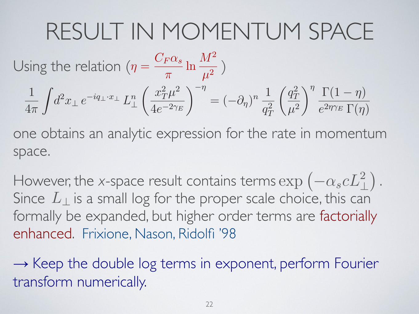
RESULT IN MOMENTUM SPACEUsing the relation ( )

one obtains an analytic expression for the rate in momentum space.

However, the x-space result contains terms . Since .is a small log for the proper scale choice, this can formally be expanded, but higher order terms are factorially enhanced. Frixione, Nason, Ridolfi ’98

→ Keep the double log terms in exponent, perform Fourier transform numerically.

where

ηF (M2, µ) =CF αs

πln

M2

µ2(56)

counts as an O(1) quantity as long as µ2 ! M2.

4.2 Fourier transformation – a first analysis

Our last task is to perform the Fourier transformation (23) from xT space to transverse-momentum space. Since all our functions depend on xT either via a power, like in (55), or viathe logarithm L⊥ defined in (30), it suffices to consider the relation

1

4π

∫

d2x⊥ e−iq⊥·x⊥ Ln⊥

(

x2T µ2

4e−2γE

)−η

= (−∂η)n 1

q2T

(

q2T

µ2

)η Γ(1 − η)

e2ηγE Γ(η). (57)

While qT serves as an infrared regulator, the integral converges in the ultraviolet, for xT → 0,only as long as η < 1. In our formulae below we will always assume that the conditionηF (M2, µ) < 1 is fulfilled. For M = MZ or MW , for example, this implies that µ should belarger than about 2GeV. Note that the higher-derivative terms in (57) are accompanied bypowers of 1/(1 − η), so that for η very close to 1 a reorganization of the perturbative seriesbecomes necessary. This will be discussed in detail in a forthcoming article [39].

Using the above result, we obtain a closed-form expression for the resummed hard-scatteringkernels, which reads

Cqq→ij(z1, z2, q2T , M2, µ) =

∣

∣CV (−M2, µ)∣

∣

2Iq←i(z1,−∂η, αs) Iq←j(z2,−∂η, αs)

× Eqq(−∂η, αs, ηF )1

q2T

(

q2T

µ2

)η Γ(1 − η)

e2ηγE Γ(η)

∣

∣

∣

∣

η=ηF

,(58)

where ηF ≡ ηF (M2, µ), and the arguments of the Ii←j(z, L⊥, αs) functions are those shown in(39). It is understood that for |CV |2 one uses the resummed expression in (50). All remainingquantities have perturbative expansions in powers of αs = αs(µ) free of large logarithms. Inwriting the above result we have introduced the function

Eqq(L⊥, αs, η) = exp[

− L⊥Fqq(L⊥, αs) − η fqq(L⊥, αs)]

= 1 −αs

4π

[

ΓF0 L2

⊥ + η

(

β0

2L2⊥ +

ΓF1

ΓF0

L⊥ +dq

2

ΓF0

)]

+ O(α2s) ,

(59)

which is completely determined in terms of Fqq. The two-loop coefficients dq2 and ΓF

1 enter herealready at next-to-leading order in αs. For a consistent resummation at NNLL order (or next-to-leading order in RG-improved perturbation theory), we need the one-loop expressions forthe matching coefficients CV and Ii←j, the two-loop expression for the exponent Fqq, the two-loop expression for the anomalous dimension γq, and the three-loop cusp anomalous dimensionand β function. All of these ingredients are known.

18

Cqq→ij(z1, z2, q2T , M2, µ) =

∣

∣CV (−M2, µ)∣

∣

2 1

4π

∫


(

x2T M2

4e−2γE

)−Fqq(x2

T ,µ)


2T , µ)

(23)

µ = µb = 2e−γE x−1⊥

µ = qT

(24)


A(3) = ΓF2 + 2β0d

q2 = 239.2 − 652.9 #= ΓF

2 (25)

exp(

−αscL2⊥

)

(26)

4

Cqq→ij(z1, z2, q2T , M2, µ) =

∣

∣CV (−M2, µ)∣

∣

2 1

4π

∫


(

x2T M2

4e−2γE

)−Fqq(x2

T ,µ)


2T , µ)

(23)

µ = µb = 2e−γE x−1⊥

µ = qT

(24)


A(3) = ΓF2 + 2β0d

q2 = 239.2 − 652.9 #= ΓF

2 (25)

exp(

−αscL2⊥

)

(26)

L⊥

4

Cqq→ij(z1, z2, q2T , M2, µ) =

∣

∣CV (−M2, µ)∣

∣

2 1

4π

∫


(

x2T M2

4e−2γE

)−Fqq(x2

T ,µ)


2T , µ)

(23)

µ = µb = 2e−γE x−1⊥

µ = qT

(24)


A(3) = ΓF2 + 2β0d

q2 = 239.2 − 652.9 #= ΓF

2 (25)

exp(

−αscL2⊥

)

(26)

η =CFαs

πln

M2

µ2(27)

L⊥

4

22

BEHAVIOR AT VERY LOW .For moderate qT, the natural scale choice is μ = qT. This is no longer true at very small qT. Detailed analysis shows that near qT ≈ 0 the Fourier integral is dominated by

Small scale qT drops out of integral! Spectrum is perturbative even at very low qT! Parisi and Petronzio ’80

We choose for general qT.

Cqq→ij(z1, z2, q2T , M2, µ) =

∣

∣CV (−M2, µ)∣

∣

2 1

4π

∫


(

x2T M2

4e−2γE

)−Fqq(x2

T ,µ)


2T , µ)

(23)

µ = µb = 2e−γE x−1⊥

µ = qT

(24)


A(3) = ΓF2 + 2β0d

q2 = 239.2 − 652.9 #= ΓF

2 (25)

exp(

−αscL2⊥

)

(26)

η =CFαs

πln

M2

µ2(27)

qT

L⊥

4

Cqq→ij(z1, z2, q2T , M2, µ) =

∣

∣CV (−M2, µ)∣

∣

2 1

4π

∫


(

x2T M2

4e−2γE

)−Fqq(x2

T ,µ)


2T , µ)

(23)

µ = µb = 2e−γE x−1⊥

µ = qT

(24)


A(3) = ΓF2 + 2β0d

q2 = 239.2 − 652.9 #= ΓF

2 (25)

exp(

−αscL2⊥

)

(26)

η =CFαs

πln

M2

µ2(27)

qT

L⊥

〈x−1T 〉 = q∗ = M exp

(

−π

2CF αs(q∗)

)

= 1.78 GeV for M = MZ (28)


4

Cqq→ij(z1, z2, q2T , M2, µ) =

∣

∣CV (−M2, µ)∣

∣

2 1

4π

∫


(

x2T M2

4e−2γE

)−Fqq(x2

T ,µ)


2T , µ)

(23)

µ = µb = 2e−γE x−1⊥

µ = qT

(24)


A(3) = ΓF2 + 2β0d

q2 = 239.2 − 652.9 #= ΓF

2 (25)

exp(

−αscL2⊥

)

(26)

η =CFαs

πln

M2

µ2(27)

qT

L⊥

〈x−1T 〉 = q∗ = M exp

(

−π

2CF αs(q∗)

)

= 1.75 GeV for M = MZ (28)


λ =pT

M(29)

nµ ∼pµ

p0

nµ ∼pµ

p0

4

23

NUMERICAL RESULTS

Preliminary: no matching to fixed order, narrow width approximation, no photon contribution.

0 5 10 15 200

5

10

15

20

25

qT

dΣ dqT

�pb�GeV� NLL

NNLL

Figure 2: The qT spectrum of Z bosons at the Tevatron Run II. The bands are obtained by varyingµF and µR (left panel) and Q (right panel) as described in the text.

lines) results. In the left panel we consider variations of the renormalization and factorizationscales. The bands are obtained by varying µR and µF as previously described in this section.We note that, in the region of small and intermediate transverse momenta (qT ∼< 30 GeV), theNNLL+NLO and NLL+LO bands overlap. This feature, which is not present in the case of thefixed-order perturbative results at LO and NLO (see Figs. 2 and 3 in Ref. [24]), confirms theimportance of resummation to achieve a stable perturbative prediction. In the region of small andintermediate values of qT , the main difference between the NNLL+NLO and NLL+LO predictionsis in the size of the scale variation bands. Going from NLL+LO to NNLL+NLO accuracy, weobserve a reduction of the scale dependence from ±4% to ±3% at the peak, from ±7% to ±3%at qT ∼ 20 GeV, and from ±7% to ±5% at qT ∼ 50 GeV. We point out that the qT region whereresummed perturbative predictions are definitely significant is a wide region from intermediateto relatively-small (say, close to the peak of the distribution) values of qT . In fact, at very smallvalues of qT (e.g. qT ∼< 5 GeV) the size of non-perturbative effects is expected to be important,while in the high-qT region (e.g. qT ∼> 60 GeV) the resummation of the logarithmic terms cannotimprove the predictivity of the fixed-order perturbative expansion. The inset plot in the left panelof Fig. 2 shows the region from intermediate to large values of qT . At large qT , the NLL+LOand NNLL+NLO results deviate from each other, and the deviation increases as qT increases. Aspreviously stated, this behaviour is not particularly worrying since, in the large-qT region, theresummed results loose their predictivity and can (should) be replaced by customary fixed-orderresults.

In the right panel of Fig. 2 we consider resummation scale variations. The bands are ob-tained by fixing µR = µF = mZ and varying Q between mZ/4 and mZ . Performing variationsof the resummation scale, we can get further insight on the size of yet uncalculated higher-orderlogarithmic contributions at small and intermediate values of qT . We find that the scale depen-dence at NNLL+NLO (NLL+LO) is about ±5% (±12%) in the region of the peak, and about±5% (±16%) in the region where qT ∼ 20 GeV. We note that in a wide region of qT values,5 GeV∼<qT ∼< 50 GeV, the resummation scale dependence is reduced by, roughly, a factor of 2 ingoing from the NLL+LO to the NNLL+NLO result. Comparing the left and right panels of Fig. 2,

7

24

LO

bands from scale variation by factor 2

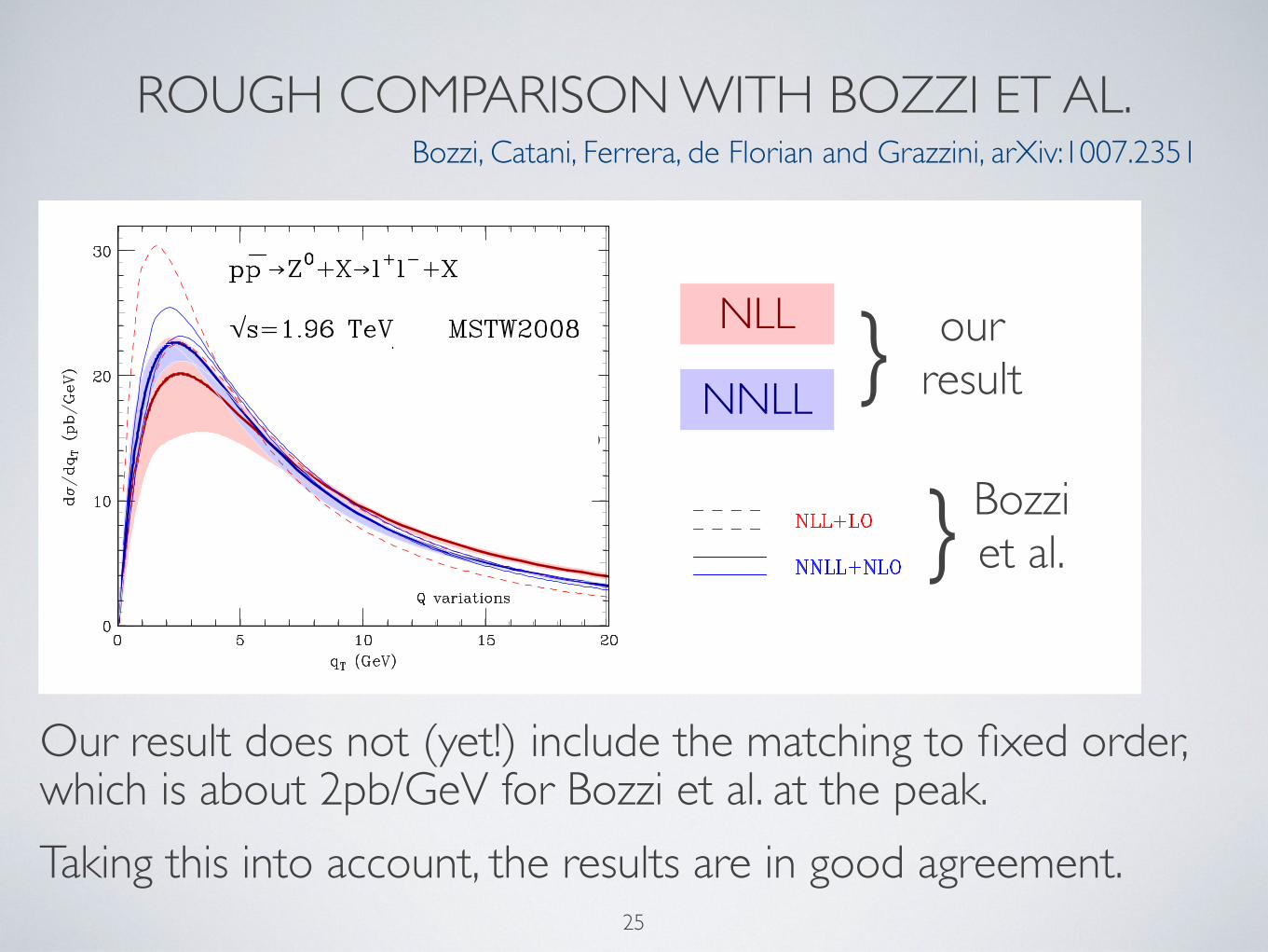
ROUGH COMPARISON WITH BOZZI ET AL.

Our result does not (yet!) include the matching to fixed order, which is about 2pb/GeV for Bozzi et al. at the peak.

Taking this into account, the results are in good agreement.

Bozzi, Catani, Ferrera, de Florian and Grazzini, arXiv:1007.2351

0 5 10 15 200

5

10

15

20

25

30




7




7

NLL

NNLL}

}

our result

Bozzi et al.




7

25

COLLINS SOPER STERMAN FORMULA

• The low scale is , and we set .

• Landau-pole singularity in the Fourier transform. To use the formula, one needs additional prescription to deal with this.

Cqq→ij(z1, z2, q2T , M2, µ) =

∣

∣CV (−M2, µ)∣

∣

2 1

4π

∫


(

x2T M2

4e−2γE

)−Fqq(x2

T ,µ)


2T , µ)

(23)

µ = µb = 2e−γE x−1⊥

µ = qT

(24)


A(3) = ΓF2 + 2β0d

q2 = 239.2 − 652.9 #= ΓF

2 (25)

exp(

−αscL2⊥

)

(26)

η =CFαs

πln

M2

µ2(27)

qT

L⊥

〈x−1T 〉 = q∗ = M exp

(

−π

2CF αs(q∗)

)

= 1.75 GeV for M = MZ (28)


λ =pT

M(29)

nµ ∼pµ

p0

nµ ∼pµ

p0

d3σ

dM2 dq2T dy

=4πα2

3NcM2s

1

4π

∫


∑

q

e2q

∑

i=q,g

∑

j=q,g

∫ 1

ξ1

dz1

z1

∫ 1

ξ2

dz2

z2

× exp

{

−∫ M2

µ2

b

dµ2

µ2

[

lnM2

µ2A

(

αs(µ))

+ B(

αs(µ))

]

}

×[

Cqi

(

z1, αs(µb))

Cqj

(

z2, αs(µb))


(ξ2/z2, µb) + (q, i ↔ q, j)

]

,

4

×[

Cqi

(

z1, αs(µb))

Cqj

(

z2, αs(µb))


(ξ2/z2, µb) + (q, i ↔ q, j)

]

,


5

×[

Cqi

(

z1, αs(µb))

Cqj

(

z2, αs(µb))


(ξ2/z2, µb) + (q, i ↔ q, j)

]

,


5

26

If adopt the choice in our result reduces to CSS formula, provided we identity

Use these relations to derive unknown three-loop coefficient, necessary for NNLL resummation

Not equal to the cusp anom. dim. as was usually assumed!

RELATION TO CSS

Cqq→ij(z1, z2, q2T , M2, µ) =

∣

∣CV (−M2, µ)∣

∣

2 1

4π

∫


(

x2T M2

4e−2γE

)−Fqq(x2

T ,µ)


2T , µ)

(23)

µ = µb = 2e−γE x−1⊥

µ = qT

(24)


4

anomaly contributionfind

A(

αs

)

= ΓFcusp(αs) −

β(αs)

2

dg1(αs)

dαs,

B(

αs

)

= 2γq(αs) + g1(αs) −β(αs)

2

dg2(αs)

dαs,

Cij

(

z, αs(µb))

=∣

∣CV

(

− µ2b , µb

)∣

∣ Ii←j

(

z, 0, αs(µb))

,

(72)

where

g1(αs) = F (0, αs) =∞

∑

n=1

dqn

(αs

4π

)n,

g2(αs) = ln∣

∣CV (−µ2, µ)∣

∣

2=

∞∑

n=1

eqn

(αs

4π

)n.

(73)

The one-loop coefficients are dq1 = 0 and

eq1 = CF

(

7π2

3− 16

)

. (74)

The two-loop coefficient dq2 has been given in (49), while eq

2 can be extracted from the resultscompiled in [31], however it contributes to B(αs) at O(α3

s) only. We have checked that therelations in (72) are compatible with our perturbative results.

Note that according to (72) the coefficient A in the CSS formula differs from the cuspanomalous dimension starting at three-loop order, and the coefficient B differs from the quarkanomalous dimension 2γq starting at two-loop order.2 The first non-zero deviations are (hereA(n) and B(n) denote the n-th order coefficients in the expansion in powers of αs/(4π))

A(3) = ΓF2 + 2β0d

q2 , B(2) = 2γq

1 + dq2 + β0e

q1 . (75)

The two-loop expression for B(αs) was obtained a long time ago in [6], while for gluon-initiatedprocesses such as Higgs-boson production the corresponding coefficient was calculated in [7].Using these results, we have derived the anticipated relation (49). Inserting the coefficientsdq,g

2 into (75), we obtain the coefficient A(3), which up to now was the last missing ingredientfor a full NNLL resummation of the qT spectrum. In the literature it is commonly assumedthat A(3) = ΓF

2 (see e. g. [21, 22]), which is true for soft gluon resummation, but our resultsshow that for transverse-momentum resummation an extra contribution arises because of thecollinear anomaly. Numerically, for the quark case with nf = 5, we find ΓF

2 = 239.2 whileA(3) = −413.7, so the extra term is much larger than the contribution from the cusp anomalousdimension and has opposite sign. It will be interesting to see how this changes the numericalpredictions for the spectrum. Note also that, due to Casimir scaling, in the gluon case a similarsituation but with larger coefficients occurs, and we find ΓF

2 = 538.2 while A(3) = −930.8.

2The first relation in (72) can be found, in almost precisely this form, in equation (3.13) of [4]. For reasonsthat are not known to us, the fact that A "= ΓF

cusp is nevertheless largely ignored in the literature.

21

find

A(

αs

)

= ΓFcusp(αs) −

β(αs)

2

dg1(αs)

dαs,

B(

αs

)


2

dg2(αs)

dαs,

Cij

(

z, αs(µb))

=∣

∣CV

(

− µ2b , µb

)∣

∣ Ii←j

(

z, 0, αs(µb))

,

(72)

where

g1(αs) = F (0, αs) =∞

∑

n=1

dqn

(αs

4π

)n,

g2(αs) = ln∣

∣CV (−µ2, µ)∣

∣

2=

∞∑

n=1

eqn

(αs

4π

)n.

(73)


eq1 = CF

(

7π2

3− 16

)

. (74)





A(3) = ΓF2 + 2β0d

q2 , B(2) = 2γq

1 + dq2 + β0e

q1 . (75)





2 = 538.2 while A(3) = −930.8.



21

find

A(

αs

)

= ΓFcusp(αs) −

β(αs)

2

dg1(αs)

dαs,

B(

αs

)


2

dg2(αs)

dαs,

Cij

(

z, αs(µb))

=∣

∣CV

(

− µ2b , µb

)∣

∣ Ii←j

(

z, 0, αs(µb))

,

(72)

where

g1(αs) = F (0, αs) =∞

∑

n=1

dqn

(αs

4π

)n,

g2(αs) = ln∣

∣CV (−µ2, µ)∣

∣

2=

∞∑

n=1

eqn

(αs

4π

)n.

(73)


eq1 = CF

(

7π2

3− 16

)

. (74)





A(3) = ΓF2 + 2β0d

q2 , B(2) = 2γq

1 + dq2 + β0e

q1 . (75)





2 = 538.2 while A(3) = −930.8.



21

Cqq→ij(z1, z2, q2T , M2, µ) =

∣

∣CV (−M2, µ)∣

∣

2 1

4π

∫


(

x2T M2

4e−2γE

)−Fqq(x2

T ,µ)


2T , µ)

(23)

µ = µb = 2e−γE x−1⊥

µ = qT

(24)


A(3) = ΓF2 + 2β0d

q2 = 239.2 − 652.9 #= ΓF

2 (25)

4

27

CONCLUSION• Have performed a factorization analysis of the Drell-Yan cross section

at low transverse momentum and derived a resummed result for the spectrum, free of large logarithms

• No Landau-pole ambiguity. Have analytic expression in momentum space, which allows for simple matching to fixed order.

• Reduces to the known CSS result for a special scale choice.

• Have derived unkown three-loop coefficient A(3) , the last missing piece needed for NNLL accuracy.

• The product of two transverse PDFs is well defined but has anomalous dependence on the large momentum transfer

• we show that this dependence exponentiates

• Phenomenological analysis at NNLL+NLO is in progress.

28

Documents

DRELL-YAN PRODUCTION AT SMALL QT