Embed Size (px)
Citation preview

GR-87-2
DRAINAGE FROM SLOPING LAND USING OBLIQUE DRAINS
February 1987 Engineering and Research Center
U.S. Department of the Interior Bureau of Reclamation
Division of Research and Laboratory Services
Hydraulics Branch

7-2090 (4-81) Bureau of Ree lamat ion
7.
1. R E P O R T NO. '
GR-87-2 4. T I T L E AND S U B T I T L E
Drainage From Sloping Land Using Oblique Drains
9.
12.
AUTHOR(S)
E. James Carlson
P E R F O R M I N G O R G A N I Z A T I O N NAME AND ADDRESS
Bureau of Reclamation Engineering and Research Center Denver, CO 80225
SPONSORING A G E N C Y NAME AND ADDRESS
Same
15. S U P P L E M E N T A R Y NOTES
REPORT STANDARD TITLE PAGE 3. R E C I P I E N T ' S C A T A L O G NO.
5. R E P O R T D A T E
February 1987 6. P E R F O R M I N G O R G A N I Z A T I O N CODE
D-1530
P E R F O R M I N G O R G A N I Z A T I O N R E P O R T NO.
GR-87-2
10. WORK UNIT NO.
11. C O N T R A C T OR G R A N T NO.
13. T Y P E OF R E P O R T AND PERIOD C O V E R E D
14. SPONSORING A G E N C Y CODE
DIBR
Microfiche and/or hard copy available at the E&R Center, Denver, Colorado
16. A B S T R A C T
A sandtank model study of drainage from sloping land using oblique drains was made in a 60-ft-long (18.29 m), 2-ft-wide (610 ram), and 2½-ft-deep (762 ram) flume. The oblique drains were tested at angles of 90, 45, 30 and Odegrees to the water table gradient. Water table gradients of O, 5, 7½, and 10 percent were tested in the study. It was apparent from the test results that the narrow flume produced boundary effects which would not permit application of test results to oblique drains on agricultural fields. However, the laboratory test results are a valuable contribution to the study of oblique drains and can be used to verify future three-dimensional mathematical models.
17. K E Y WORDS AND DOCUMENT ANALYSIS
O. D E S C R I P T O R S ' " hydraulic models/drainage/drain spacing/water table gradient/computer programs/percolation/ground water recharge/deep percolation/slopes/subsurface drains/ hydraulic conductivity/permeability
b. I D E N T I F I E R S - - Oblique d r a i n s
c. COSATI Fie(d/Group 13M COWRR: 1313.1 SRIM:
18. D I S T R I B U T I O N S T A T E M E N T 19. S E C U R I T Y C LASS (THIS REPORT)
UNCLASSIFIED 20. S E C U R I T Y CLASS
(THIS PAGE) UNCLASSIFIED
21. NO. OF PAGE!
44 22. PRICE
I I I I I I I I I I I I I I I I I I I
M
GR-87-2
DRAINAGE FROM SLOPING LAND USING OBLIQUE DRAINS
by
E. James Carlson
Hydraulics Branch Division of Research and Laboratory Services
Engineering and Research Center Denver, Colorado
February 1987
UNITED STATES DEPARTMENT OF THE INTERIOR -k BUREAU OF RECLAMATION

ACKNOWLEDGMENTS
The studies were conducted by the author under the general supervision and review of D. L. King, former Chief of t he Hydraulics Branch. This report was reviewed by E. R. Zeigler; T. J. Rhone, Head, Hydraulic Structures Section; and P. H. Burgi, Chief, Hydraulics Branch,
As the Nation's principal conservation agency, the Department of the Interior has responsibility for most of our nationally owned public lands and natural resources. This includes fostering the wisest use of our land and water resources, protecting our fish and wildlife, preserv- ing the environmental and cultural values of our national, parks and historical places, and providing for the enjoyment of life through out- door recreation. The Department assesses our energy and mineral resoumes and works to assure that their development is in the best interests of all our people. The Department also has a major respon- sibility for American Indian reservation communities and for people who live in Island Territories under U.S, Administration.
The information contained in this report regarding commercial" prod- ucts or firms may not be used for advertising or promotional purposes and is not to be construed as an endorsement of any product or firm by the Bureau of Reclamation.
I I I I I i I | !
I i !
i
I I I I I I

I I I I I I I i I ,I I I I I I I I I I
CONTENTS
Page
In t roduc t i on . . . . . . . . . . . . . . . . . . . . . . .................................................................... : ....................................... 1
S lop ing sand tank (f lume) m o d e l ....................................................................... ; . . . . . . . . . . . . . . . . . . . . . . . . . . . 2 S imu la ted agr icu l tura l dra ins ........................................................................ - . . . . . . . . . . . . . . . . . . . . . . . . . . . . . 2 F loor dra ins ......................................................... .................................................................... 2 P iezome te r we l l s ...................................................................................................................... 3 W a t e r rec i rcu la t ion s y s t e m ....................................................................................................... 3 Recharge m o d u l e s .............................................. : .................................................................... 4 W a t e r recharge measu r i ng s y s t e m ............................................................................................ 4 M e a s u r e m e n t o f w a t e r tab le .............................................................. ....................................... 4 A q u i f e r sand .. . . . . . . . . . . ....................................... • ......................................................................... 5
Genera l p lan o f t es t s ............................................................................. . ...................................... 5 Var ia t ion in w a t e r tab le s lope .... :. . . . . . . . . . . . . . . . . . . . . . .......................................................................... 7 Recharge (deep perco la t ion ) ..... ....: . . . . . . . . . . . . . . . : ............................................................................. 7 Drain d ischarge m e a s u r e m e n t s ................................................................................................. 7
Drain tes t da ta .. . . . . . . . . . . • .......................................................................................... . . . . . . . . . . . . . . . . . . . . .
Genera l ................................................................................................................. . . . . . . . . . . . . . . . . . Data f r o m A (90 -degree) dra ins ............................................................................................... Data f r o m B (45 -deg ree ) dra ins ................................................................................................ Data f r o m C (30 -degree) dra ins ................................................................................................ Data f r o m D (O-degree) dra ins ........................................ : ........................................... . . . . . . . . . . . . . .
8 8 9 9
10 10
S u m m a r y and ana lys is o f t es t s ..................................................................................................... 11
In f i l t ra t ion recharge vs. dra in d i scharge ......................................................................................... 1 2
M a x i m u m w a t e r tab le b e t w e e n dra ins ........................................................................................... 1 2
Conc lus ions and r e c o m m e n d a t i o n s ............................................................................................... 1 3
Bib l i og raphy ................................................................................................................................. 1 3
APPENDIXES
Append ix A C o m p u t e r p r o g r a m E J C 1 6 M fo r d e t e r m i n i n g m a x i m u m w a t e r tab le he igh t b e t w e e n
agr icu l tura l p ipe dra ins ................................................................................................ 15 B C o m p u t e r p r o g r a m E J C 2 0 M fo r d e t e r m i n i n g pe rmeab i l i t y o f aqu i fe r w h e n m a x i m u m w a t e r
t ab le he igh t b e t w e e n agr icu l tura l p ipe dra ins is k n o w n ................................................... 19
FIGURES
Figure Page
• 1 Hydrau l ic m o d e l s lop ing f l ume used fo r ob l i que drain t es t s ................................................ 2 4 2 Tes t f l ume t i l ted t o i ts m a x i m u m s lope , 12 pe rcen t ........................................................... 2 4 3 Des igna t i ons and l oca t i ons o f dra ins and p i e z o m e t e r s in t es t f l ume .................................... 2 5 4 W a t e r rec i rcu la t ion s y s t e m : ............................................................................................. 2 6 5 W a t e r recharge m o d u l e s ..................................................................... . . . . . . . . . . . . . . . . . . . . . . . . . . . . . 2 6 6 Pressure measur ing and reco rd ing s y s t e m fo r p i e z o m e t e r s ................................................ 2 6 7 S ieve ana lys is o f sand used fo r aqu i fe r and drain e n v e l o p e mater ia l .................................... 2 7

C O N T E N T S - C o n t i n u e d
8 Cross section showing the water table between drains .............................................. ....... 27 9 Locations of piezometers for A drains ....................... .~ ...................................................... 28
10 Locations of piezometers for B drains .............................................................................. 29 11 Locations of piezometers for C drains .............................................................................. 30 12 Locations of piezometers for D drains .............................................................................. 31
Table
1 2 3 4 5
6
TABLES
Description of table column headings ............................................................................... 32 Hydraulic model data for A drains (Alpha = 90 degrees to water table gradient) ................. 33 Hydraulic model data for B drains (Alpha = 45 degrees to water table gradient) ................. 35 Hydraulic model data for C drains (Alpha = 30 degrees to water table gradient) ............ ' ..... 37 Hydraulic model data for D drains (Alpha = 0 degrees to water table gradient) ................... 39 Hydraulic model data, infiltration recharge compared with drain discharge for all drain sets
and all flume slopes ..................................................................................................... 41 Hydraulic model data and data computed using programs EJC20M and EJC16M. Maximum
water table heights between adjacent drains for all drains sets and flume slopes ............ 42
iv
I I I I I I I I I I I I I I I I I I I

I I I I I i I I I I I I i I I I I I
INTRODUCTION
In most agricultural lands in the arid Western United States, where applied irrigation water is
re~quired for crop production, drainage capability must be available. Practically all arid soils require
more water than that used by the Crops to maintain the salt balance in the soil and to achieve
high plant productivity. Drainage of the excess water can be provided by open channel drains, by
natural creeks or ditches, or by buried pipe (or tube) drains. Buried pipe drains are normally used
so that the land above the drains can be cultivated.
Most agricultural land chosen to grow valuable food or forage crops has a surface slope, whether
natural or artificial, which provides natural storm runoff drainage. On arid land, where irrigation is
required to grow crops, the excess water leaching the root zone must be removed for salt control.
Such drainage is necessary to prevent the water table from encroaching on the root zone, thus
making the land unproductive. A pipe drainage and collection system is usually provided to ensure
that the water table stays below the root zone.
Pipe drains are installed at right angles to the water table gradient, where possible, to serve as
relief or interceptor drains to maintain the water table at the desired level. Interceptor drains on
sloping land, installed at right angles to the water table gradient, provide the most hydraulically
efficient drainage. However, it is often necessary to install drains at an oblique angle to the water
table gradient. Unsymmetrical property lines, odd shapes of fie!ds, varying topography, and natural
drainage conditions sometimes necessitate the installation of oblique drains.
PRESS (Program Related Engineering and Scientific Studies) coordinated with the Drainage and
Groundwater Branch, were conducted by the Hydraulics Branch to study drainage from level and
sloping land (PRESS allocation No. DR-414). The tests were conducted with drains placed at a
right angle to the water table gradient. After the initial research was Completed and reports [1,2] °
were published, further research was conducted, using the excellent research facilities in place,
to learn about the technique for using oblique drains on sloping land.
Although some problems were apparent in studying the three-dimensional condition with a two-
dimensional test facility, several series of tests were conducted and valuable information was
obtained.
Most drainage installations constructed where the land is sloping require drains oblique to the
water table gradient. A major question was to determine the most efficient spacings of these
* Numbers in parentheses refer to entries in the bibl iography.

oblique drains. Without guidelines, drain spacings could be less than the optimum for efficient
operation, making the drainage system cost more than necessary.
SLOPING SAND TANK (FLUME) MODEL
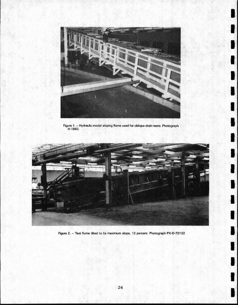
The sloping sand tank flume (figs. 1 and 2) used for the study was 60 feet (18.29 m) long, 2 feet (610 mm)
wide, and 21/2 feet (762 mm) deep. Plastic panels, ~-inch (9.53 mm) thick, formed one side of the flume.
For ease in tilting, the flume was built on two 16WF36 continuous steel beams, each supported at two
points. The downslope beam support was a pivot, and the upslope support was the lifting mechanism.
Supports were spaced along the beams to give equal deflection at the ends and the center of the flume.
The design load on the beams was 900 Ib/ft (1339.3 kg/m), 450 Ib/ft (669.7 kg/m) on each beam; this
load considered the weight of the flume and attached test equipment, the sand, water, beams, and the
people standing on the walkway on the side of the flume. One end of the flume was lifted to achieve the
desired slope by two 8-ton (7.26-metric ton) motorized chain hoists. Templates were used tO determine
the flume slope. For safety, screwjacks were placed under the cross beams provided for the upslope lifting
hoists. Because of headroom limitations, the maximum slope obtainable was about 12 percent (about 6
degrees 50 minutes).
Simulated Agricultural Drains
To simulate pipe drains, %-inch (15.9-mm) o.d. by V2-inch (12:7-mm) i.d. plastic tubes were used.
These plastic tubes were slotted with a band saw to simulate perforated plastic pipe drains used
in the field. The flume length was divided into four zones (A, B, C, and D), whose respective drains
were installed at angles of 90, 45, 30 and 0 degrees to the water table gradient. The drains were
installed level across the flume and longitudinally on a plane 2.0 feet (0.61 mm) above the flume
floor when the flume was set to the zero Slope position (see fig. 3). After the drains were installed,
their placement was checked with an engineer's level and rod. The discrepancies between levels
of the drains and between their distances above the flume floor were within a few hundredths of
an inch, which was considered well within the overall accuracy of the tests.
Floor Drains
Eleven floor drains, used only to drain and fill the flume at the end of a series of tests, were placed
along the centerline of the flume. The first drain was 1 foot (305 mm) from the downslope end.
The drains were spaced 6 feet (1.83 m) apart with exception of the last two drains on the upslope
end, which were 4 feet (1.22 m) apart; this caused the last drain to be 1 foot (305 ram) from the
2
I I, I I i I I I I !
I I I I I I I I
upslope end of the flume. The floor drains were made from ½-inch (12.7-mm) galvanized pipe
with the vertical end of each drain passing through the floor of the flume. A valve in each drainline
led to a common 1 ½-inch (38.1-mm) pipe manifold beside the flume floor that extended the entire
length of the flume. Each floor drain was covered by 100-mesh screen and a i-inch (25.4-mm)
thick layer of No. 16 medium sand.
Piezometer Wells
Piezometer wells were used to define the height of the water table above and between adjacent
pairs of drains. They were made of %-inch (15.9-mm) o.d. by ½-inch (12.7-mm) i.d. plastic tubes
7½ ~ inches (190.5m-mm) long. The bottom end of each tube was plugged, and the bottom 2
inches (50.8 mm) was slotted in the same manner as the drain tubes. A small cylinder of 100 °
mesh bronze screen was placed inside each piezometer to keep out the sand. The bottom of each
piezometer well was set 1/2 inch (12.7 mm) below the centerline of the plane of the drains.
The water table was measured between four adjacent pairs of drains, 3A to 7A, for the 90-degree
configuration; between three adjacent pairs of drains, 5B to 8B, for the 45 degree configuration;
between three adjacent pairs of drains, 5C to 8C, for the 30- degree configuration; and between
two adjacent drains, right and left between collectors 2D and 4D, for the 0-degree configuration
(see fig. 3). The water table height was measured at right angles to adjacent drains for each drain
configuration.
The 90-degree drains were located between stations 0 and 12 feet (0 and 3.66 m) in the flume,
the 45-degree drains between stations 12 and 27 feet (3.66 and 8.23 m), the 30-degree drains
between stations 27 and 45 feet (8.23 and 13.72 m), and the O-degree drains between stations
45 and 60 feet (13.72 and 18.29 m). As shown on figure 3, water table measurements in each
zone were made between adjacent drains that would receive a minimum of influence from other
zones or from the vertical end drains. The water table measurements were made where a uniform
flow net would be established.
One-quarter-inch plastic tubing connected each piezometer tube to a scanivalve which, in turn,
was connected to a sensitive pressure transducer and digital voltmeter and recorder. The ~scani-
vaIvehad 52 piezometer connections. All of the piezometers for each of the A, B, and C drain
sets could be read without changing the piezometer connections.
Water Recirculation System
The water supply for the flume was a closed-circuit flow system. Recharge water was pumped
from a covered storage reservoir, 7 by 7 by 4 feet (2.13 by 2.13 by 1.22 m) deep, throughl a

manifold piping system to plastic recharge modules (figs. 4 and 5). The recharge water passed
through a stainless steel screen filter and a 11/z-inch (38.1-mm) plastic pipe manifold to vertical
½-inch (12.7-mm) plastic pipes. Each of the 10 pipes fed a separate recharge module. Drainage
water from all drains was collected in a galvanized trough, from which it flowed into a tank at the
downslope end of the 60-foot (18.29 m) flume, where it was pumped back to the covered storage
reservoir.
The test facility was not in a temperature- or humidity-controlled environment and, consequently,
followed the ambient temperature and humidity of the laboratory. However, because of the large
amount of water and sand used, temperature changes in the model were very small and very slow
and had no effect on the test results.
Recharge Modules
Each recharge module consisted of three plastic tubes, ½ inch (12.7 mm) o.d. by z/e inch (9.52 mm)
i.d. by 6 feet (1.83 m) long. The tubes were placed side byside, 0.70 foot (213 mm) apart and
0.30 foot (91 mm) away from the flume walls on each side. The recharge tubes were kept horizontal
when the flume was tilted. The tubes were drilled with 12 holes, 0.020 inch (0.508 mm) in
diameter, 1 foot (305 ram) apart on the upper side of the tubes. Each hole had an inverted cup
over it. The water squirted up into the cup and then dripped onto the sand aquifer. By having the
holes on top of the tubes, air could escape and the holes did not clog with foreign matter. The
inverted cups eliminated spray as water left the ½-inch (12.7-mm) supply tubes.
Water Recharge Measuring System
In the earlier tests, the water that recharged the aquifer was measured as it flowed to each recharge
module with small stainless steel orifices and water manometers; needle valves controlled the
flow. However, in the oblique drain tests, glass rotameters made by Schutte and Koerting were
used for the recharge water measurement. The rotameters were 10 inches (254 mm) long and
were connected to the ½-inch (12.7 mm) plastic pipes with rubber hose connectors. Rotameters
were selected that would measure approximately 1.26 gal/min (0.08 I/s) to fit the range of desired
• recharge for each module. Measurements could be set much more quickly and more accurately
with the rotameters than with the small orifices used in the earlier tests.
Measurement of Water Table
The most important factor to consider when designing an agricultural drainage project is the
maximum height of the water table between drains. Therefore, very accurate measurements of
4
I I i I m I I
I I I I I I I I I I i
the water table between drains were made in the model. Piezometers were placed between drains
so the water table shape with its highest free-water surface between adjacent drains could easily
be defined.
To measure the water table between drains, a pressure measuring system was connected to the
water piezometers with ¼-inch (6.4-mm) plastic tubing. A sensitive pressure transducer with a
scanivalve (fig. 6) made it possible to •read multiple piezometer pressures quickly. Twenty-eight
piezometers were installed in the 900degree (A-drain) zone, 45 piezometers in both the 45-degree
(B-drain).and the 300degree (C-drain) zones, and 84 piezometers in the 00degree (D-drain) zone
(fig. 3). The'actual pressures were read from the transducer with a digital voltmeter and printed
on strip paper. This method Was much more rapid, accurate, and efficient than the water manom-
eter board method used in the earlier tests.
Aquifer Sand
With the exceptions described below, the flume was filled with a uniform rounded silica sand
having a medium particle size of slightly less than 0.2 mm. A sieve analysis of the sand is shown
on figure 7. A circular envelope of No. 16 medium sand, 0.1 foot (30.Smm) in outside diameter,
was placed around the pipe drains. At both ends of the flume a ½-foot (152-mm) deep layer of
No. 16 medium sand was installed to assist in determining the hydraulic conductivity of the aquifer
sand and to control the water level and water removal at the downslope end of the flume.
Hydraulic conductivity tests were conducted by measuring the discharge,'hydraulic gradient, and
cross-sectional area of water moving down the sloping flume. The average hydraulic conductivity
of several tests was 481902 feet (14.905 m) per day for the sand material installed in the flume.
During this long testing program there was no •settlement in the sand. When the sand was removed
from the flume in February 1986, it appeared to be in excellent condition. It was dense, had no
cavities, and showed no signs of algae or other foreign growth.
GENERAL PLAN OF TESTS
In the previous tests [1,2], all drains were placed at 90 degree angles to the water table gradient
(i.e., Alpha = 90 degrees in the flume). These earlier tests were conducted with 6- and 12-foot
(1.83 and 3.66 m) drain spacings. To compare drainage parameters of oblique drains with those
placed at 90 degrees to the water table gradient, it was necessary to use smaller spacings. For
the A, B, and C drains (at 90 o, 45-, and 300degree angles, respectively, to the gradient), a spacing
•5

of 1.5 feet (456 mm) along the side walls was selected. This gave drain spacings perpendicular
to the drains as follows:
Drain Angle to Perpendicular Length of drain number gradient, drain spacing, between walls,
degrees ft ft
1A-7A 90 1.50 2.00 1B-9B 45 1.06 2.83 1C-10C 30 0.75 4.00
Figure 8 is a definition sketch showing that the water table between drains is measured at a right
angle to the drains and perpendicular to the plane of the drains. This is true for all zones whether
or not the drains are oblique to the sloping water table gradient.
The D drains, which had a 0-degree angle to the water table gradient (straight down the slope),
were spaced 1.0 foot (305 mm) apart to allow the water table to rise between the drains and
adjacent to the flume wall and to make the flow net near the drains similar to a flow net in a field
installation. Five collection tubes (1D-5D) spaced 3 feet (915 mm) apart collected drain water by
gravity from the D drains and passed it through the left flume wall (looking downslope). The
collection tubes carried drain water to the outlet trough, which carried the water to the tank at
the downslope end of the flume. The collection tubes prevented the drains from being submerged,
which would have changed the flow net around the drains from normal flow conditions.
For the A drains, seven piezometers were placed along the centerline between each of four sets
of adjacent drains (3A-7A) and at right angles to the drains (fig. 9). For the B drains, 15 piezometers,
five in each of three rows, spaced 0.25 foot (76.2 mm) apart, were centered in the flume between
adjacent drains (5B-8B) and at right angles to the drains (fig. 10). The number and configuration
of piezometers for the C drains were similar to those for the B drains (fig. 11). For the D drains,
six rows of piezometers were installed between collection tubes at right angles to the drains (fig.
11).
All piezometers foreach set of drains being tested were read so the water table between drains
could be defined. Recharge water was added to the, entire flume and drains in all zones were
operating when tests were conducted for one or more sets of drains. This ensured a continuous
operating flow net over the entire flume when each set of drains was tested.
The parameters that could be varied in the model were the recharge (deep percolation) rate and
the slope of. the flume (angle Beta). The other parameters that affect drainage relationships are
the hydraulic conductivity (coefficient of permeability) of the aquifer material, the spacing of the
6

drains, the distance between the level of drains and the impermeable barrier in the geological
formation below tile agricultural land, and the sum of the drain radius plus the thickness of the
gravel envelope around it. All of these parameters were fixed in the model test setup and remained
constant'as shown below:
Radius of drains plus gravel envelope ..................................................... 0.05 feet
Distance below drains to impermeable barrier ......................................... 2.00 feet
Hydraulic conductivity (coefficient of permeability) ....................... 48.902 feet/day
Variation in Water Table Slope
The test flume was constructed so it could be raised and pivoted to give a maximum angle of 12
percent, about 6 degrees 50 minutes from the horizontal. Tests were made at 0, 5, 7½, and 10
percent to show thevariation of the water table between drains as the water table gradient varied.
As the testing progressed, the piezometer readings revealed-the three-dimensional nature of the
flow. ReCharge. (deep percolation) water applied by the recharge modules percolated vertically
downward until it reached the water table, and then flowed to the drains according to the pressure
distribution in the saturated flow net.
Recharge (Deep Percolation)
Water reaching agricultural drains that are located below the root zone is deep percolation water
that is not used by the plants. This water carries excess salts from the root zone to the drains
and prevents salt buildup in the soil. In tlie hydraulic model no agricultural plants were used and
all recharge water was deep percolation water. The rate of recharge could be varied to yield a
water table height between •drains that was high enough to allow accurate water table measure-
ments, but was not extremely close to the ground surface.
For the A, B, and C drains, recharge was maintained at approximately 7.5 cubic feet of water per
square foot per day (feet per day) (2.29m/day) to maintain a reasonable water table height for
steady flow Conditions. At this rate the drains would not become flooded. A recharge rate of
approximately 4.5 feet per day (1.37 m/day) was used for the D drains.
Drain Discharge Measurements
Discharge from pipe drains, which extended through the left wall of the flume, was measured by
collecting individual drain outflows in a graduated cylinder and timing them with a stopwatch. Each

drain discharge was collected for nearly a minute and timed to 0.1 second. Flow rates from the
drains ranged from 5 to 15 mL per second (15.26 to 45.70 ft 3 per day). Flow from the downslope
end of the flume during the sloping aquifer tests was removed by drains installed in the vertical
layer of No. 16 medium sand at the end of the flume.
DRAIN TEST DATA
General
The D drains, placed at a O-degree angle to the water table gradient, were at the limit angle of
oblique drains used for drainage, Drains placed in this configuration could not perform as true
interceptor drains, particularly for the steeper slopes, because they were parallel to the water
table gradient. On first thought, to have the drains run down the slope would seem to be the best
way to drain sloping land. But upon closer analysis of the flow net, and considering accretion
vertically from the root zone above and the water flowing according to the pressure at every point
in the saturated flow, it became obvious that drains placed at 90 degrees to the gradient are
preferable. The drain is the line sink and gravity is the driving force. Because the flow lines become
curved in three dimensions, analysis and interpretation of the data taken on the two-dimensional
model was most difficult. A three-dimensional mathematical model is needed to supplement the
two dimensional hydraulic model data.
In the hydraulic model, pressures and water levels could be measured at a point or at several
consecutive points, and the discharge could be measured from the drains or from a drain collection
system, as for the D drains. To measure differential changes in potentialin three dimensions would
require an infinite number of monitoring instruments placed very close together, an impossible
test setup. The best practical test setup used included a single pressure-measuring instrument
with a large number of piezometers placed at close intervals to define the water table between
drains, and then to measure the discharge from adjacent drains for each test.
For drains sets A and D (fig. 3), the flume simulates a slice of land parallel to the water table
gradient in a wide sloping field. The sides of the flume do not cause boundary influence to the
flow net in the A and D drains because they are perpendicular and parallel, respectively, to the
water table gradient (figs. 9 and 12). Drain sets B and C, 45 and 30 degrees, respectively, to the
gradient, have three-dimensional flow nets. Data for these oblique drains show the influence of
the flume sides, even though piezometers were installed as far as practical from the flume walls
(figs. 10 and 11). 1 "
8

Tests were conducted for the A drains by setting the recharge rate for the entire flume, then
waiting until equilibrium flow from the drains was established. Equilibrium was usually apparent
within 1 hour. Piezometer readings were made for each slope, 0, 2½, 5, 7½, and 10 percent,
using the same recharge on each set of drains for each slope setting. Piezometer connections
were then changed to the B, C, and D sets of drains, in order, and the same procedure was
followed. Drain discharge was measured for all drains in each set as data were taken to ensure
that equilibrium continued in the test. For the D drains, which were installed straight down the
slope (with a different drain collection system), a different recharge rate was required to have the
water table height within the range of the test setup.
Data From A (90-degree) Drains
There were seven drains in the A set. Twenty-eight piezometers were used between drains 3A
and 7A, seven in each space between adjacent pairs of drains. The recharge modules over the
entire flume were kept operating to maintain continuity and equilibrium.
The maximum water table height between drains was the important value for designing drain
spacings. The maximum water table heights between drains were taken from smooth curves drawn
through piezometer pressures measured.perpendicular to the plan of the drains: Recharge rate
and drain discharge were converted to recharge infiltration in feetper day over. the area of the
soil surface being considered (see tables 1 through 5).
I I I I I I I
The maximum water table height between the 90-degree A drains varied a small amount for each
slope tested. The only trend noticed was that the average height of the water table between the
A drains decreased as the water table slope increased. However, this decrease was less than the
variation in the water table between drains for a given test. The water table heights for the A
drains on a zero slope (horizontal) were within the range of experimental accuracy of the water
table heights measured when the water table was sloped 2½ to 10 percent (table 1 ).These data
showed results similar to the data obtained from previous tests [1, 2] with 6- and 12-foot (1.83 m
and 3.66 m) spacings.
Data From B (45-degree) Drains
The same recharge inflow rates were used for the B drains as for the A drains. A slightly different
area contributing to the different drain sets made the converted recharge rates differ slightly
between drain sets. The drain spacing was shorter for the B drains than for the A drains, so the
water table height above the drains was less. The average maximum water table heights above
9

the plane of the drains were very close for,slopes, 2½ to 10 percent. However, the water table
was always higher on the left side of the flume looking downslope (table 2). The influence of the
boundaries 'df the flume sides are clearly shown where the drains are truly at oblique angles to
the water table gradient. The effect is greater between drains 5B and 6B than between 6B and
7B. °
Data From C (30-degree) Drains
Because the perpendicular distance between the C drains (0.75 ft) was less than that for either
the A drains (1.50 ft) or the B drains (1.06 ft), the water table heights for the C drains were lower
(figs. 9, 10, 11 and table 3). The effect of the flume boundaries was apparent when observing
the plots of each row of piezometer pressures. However, the piezometer pressures between drains
6C and 7C had a pattern that showed the water table to be considerably lower close to drain 7C
than in the areas between drains 5C and 6C and between drains 7C and 8C. This could be caused
by drain 7C deflecting when it was installed, making the piezometer pressures lower in this location.
Although the water table was lower near drain 7C, as shown on piezometer pressure plots of 6C-
R, 6C-C, and 6C-L, the maximum water table height between drains 6C and 7C was very close
to the pattern of water table heights between drains 5C and 6C and between drains 7C and 8C.
The 30-degree angle of drains made them act more like the D drains (placed straight down the
slope) where tl~e water table built up higher the farther down the slope the water traveled before
reaching a drain outlet.
Data From D (O-degree) Drains
The water table profile for the D drains was lower toward the upslope drain exit. This is the
opposite of the profile of water table between the 90-degree A drains. For a wider drain spacing,
such as 6 and 12 feet (1.83 and 3.66 m) [2], it is more noticeable. Table 4 shows a comparison
of drain discharge from each of the five D drains and discharge from the downslope flume end
drain. As the water table slope increased from 2½ percent, discharge from the end drain increased.
Table 4 also shows the water table profile between drain exits 2D and 3D and between drain exits
3D and 4D. After water drains from 3D, the water table downslope drops abruptly. For the 10-
percent gradient, the water table drops below the plane of the drains for piezometers 1 and 2.
These data show how inefficient drains placed at a O-degree angle are for slopes above 2½ percent.
The excess end drain discharge for slopes above 2½ percent indicates flow passing downslope
between the plane of the drains and the barrier.
10
I I I i I I i I I I I i i I i I i i i

I I I I I I i I i I I I I I ! !
i i i.
SUMMARY ANDANALYSIS OF TESTS
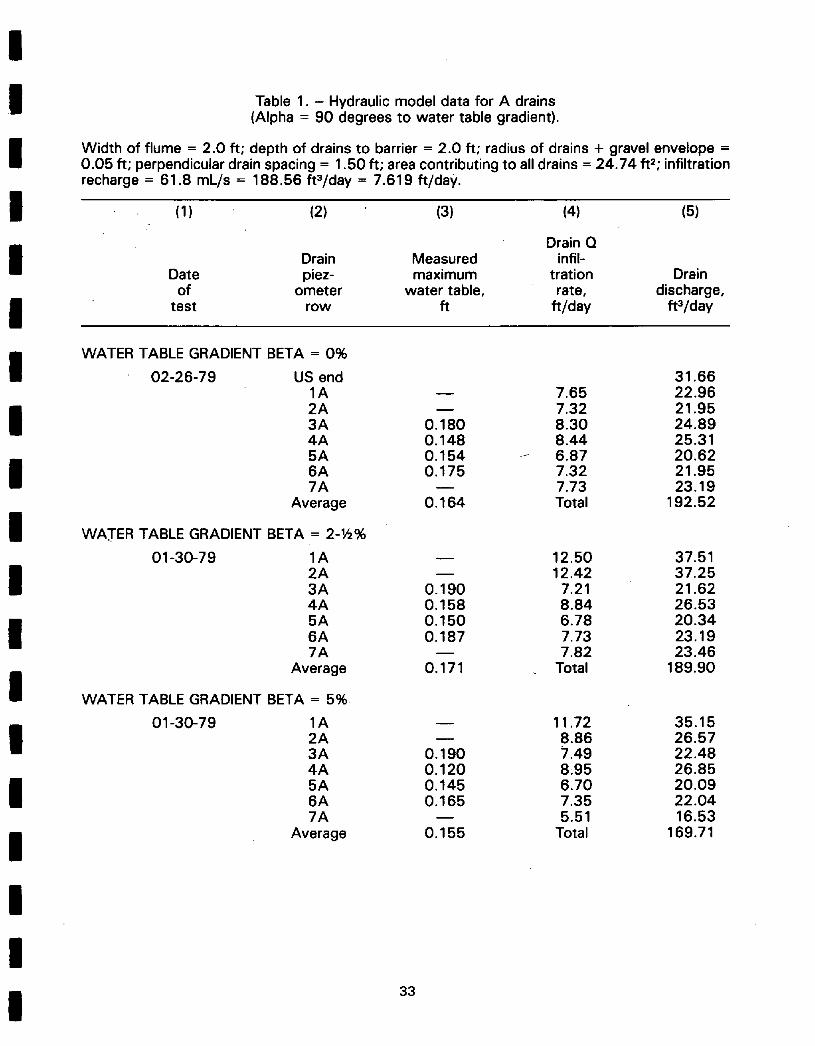
Table 1 shows the maximum water tabie heights between A drains for water table gradients 0 ,
2-½, 5, 7-½, and 10 percent. The maximum water table height between adjacent drains from
drains 3A to 7A are taken from seven piezometers between each of four pairs of adjacent drains.
Discharge rates from all seven A drains are also shown. The pattern of maximum water table
heights is similarf0r all water tablegradients. Pressures in piezometer sets 3A and 6A were higher
than those in piezometer sets 4A and 5A. Sets 4A and 5A show maximum water table heights
about 82 percent of the Water table heights in 3A and 6A. There is no apparent reason for this !
trend except the drain discharge from the next drain downslope would generally increase as the
upslope water table would increase and the drain discharge would decrease as the upslope water
table would decrease, Averaging the water table heights in the four sets of piezometers showed
that the average maximum water table heights decreased as the slope of the water table gradient
increased: 0.171 feet (52 mm) for a 2-½ percent slope and 0.144 feet (44 mm) for a 10 percent
slope.
Water table heights for the B drains .(45 degrees to the water table gradient) were higher on the
left side of the flume looking downslope, than on the right side (table 2). This trend was more
prominent for the B drains than for the C (30-degree) drains. In a large agricultural field with a
water table of uniform slope, a uniform maximum water table between drains would be expected
over the entire drained area. It is apparent that the flume side walls had a boundary influence on
the pattern of the water table between drains in the model.
The pattern of water table heights was similar for all slopes of gradient, 2-½ to 10-percent. With
accretion from uniform irrigation water, or recharge in the model study, water flowing vertically
downward would follow a flow net affected by gravityand the line sink of each drain. The B drains,
aligned at a 45-degree angle downslope to the left (fig. 10), caused the accretion water to move
to the left and build up against the left flume wall.
The discharge from each of the nine B drains is also shown in table 2. The flow varies from drain
to drain, but the pattern of each of the four slopes of water table gradient tested was the same.
Variations are very likely due to slight differences in the levels of the drains and their alignments,
or due to possible deflections of the drains in the model during installation. A similar variation in
discharges from individual drains in each drain set can be seen in the tables for each set. Upslope
drain 1B and downslope drain 9B had higher discharges than drains 2B through 8B. Excess dis-
charge in the upslope and downslope drains was apparently due to the change of pattern of drains
installed between the A and B drain sets,and between the B and C drain sets.
11
The C drains (30 degrees to the water table gradient) .had. a pattern of maximum Water table
heights between drains similar to that for the B drains, except that the water table did not build
up on the left side. Thesmall angle between the drains ancl the gradient did not have a great effect
on the flow net.
Water table heights for the D drains (0 degrees to the water table gradient) increased going
downslope from a drain collector to the next downslope drain collector. Drain discharge increased
from the upslope drain collector, 1D, to the downslope drain collector 5D. For every test consid-
erable flow reached the vertical drain at the end of the flume (table 4). It was obvious that con-
siderable flow was moving downslope in the aquifier below the plane of. the drain sets as described
below. '
,; INFILTRATION RECHARGE VS. ,DRAIN DISCHARGE
A summary of a typical set of measurements showing infiltration recharge and discharge from all
drain sets for all water table gradients tested is given in table 5. A test for the A drains with the
water table gradient set at zero slope (flume level) shows considerable flow, 31.66 ft 3 per day
(0.90 m3/day), discharging from the upslope vertical end drain. At zero slope and at 2-Fz percent
slope, a small discharge came from the upslope end drain.
As the water table gradient was increased, 5 to 10 percent, considerable fl0w from accretion to
theA-drain zone flowed down the slope under the drains. Column 5 on table 5 shows that the
difference between total infiltration and drain discharge was comParatively small. The difference
between infiltration and drain discharge for the C drains was larger, and for the D drains it increased
dramatically. '
M A X I M U M WATER,TABLE BETWEEN DRAINS
Because the perpendicular spacings between drains ,was different for each set of drains, it was
necessary to use a normalizing computation to compare water table heights. In report [ t ] the
development of a computer program, EJC16M (app. A), is described relating to the various pa-
rameters that influence drain spacing design for steady recharge conditions. Donnan's tile spacing
formula [3] was used with Hooghoudt's correction for convergence [4] in developing this computer
program. These formulas have been used extensively for drainage design in steady-state conditions
and for a first estimate for transient drainage conditions [5, 6]. The steady-state drain spacing
12
r I
I
I I I I I i I I I I. I I i I I I

I I i I I I I I I ,I I I I I I I I I I
formulas are based on the Dupuit-Forchheimer idealization, which involves the assumption that
the gradient at the water table is effective through the entire saturated thickness of an unconfined
aquifer. The drainage design parameters are the coefficient of permeability (hydraulic conductivity)
of the aquifer material, drain spacing, radius of the drain plus gravel envelope, depth between
drains and impermeable barrier, infiltration recharge (deep percolation), and the maximum water
table height between drains. The formulas are based on drainage from level land.
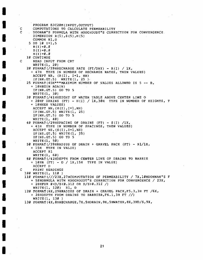
Another computer program, EJC20M (app. B), used to compute permeability when the other
variables were known, was adapted from EJC16M. Using the A-drain test for zero water table
gradient gives a permeability of 38.02 feet per day (11.59 m/day). This is less than the permeability
of 48.902 feet per day (14.91 m/day) measured in the 60-foot-long (18.29 m) flume because of
the small drain spacing and the Dupuit-Forchheimer idealization. Using a permeability of 38.02
feet per day and computing water table heights for the B, C, and D drain sets with respective
drain spacings of 1.06, 0.75, and 1.0 feet (320,229, and 305 mm) gave a way to compare water
table heights among the different oblique drains. The comparison is shown on table 6 for all drain
sets and for all water table gradients tested.
CONCLUSIONS AND RECOMMENDATIONS
/ From the data taken in the narrow, 2-foot- (610 ram) wide flume, it was apparent that the flume
sides had a boundary effect on steady-state ground water flow to oblique drains. Using the flume
data, comparable efficiencies of oblique drains could not be determined for drains installed at
various angles to the water table gradient and for a variation of the water table gradient.
A three-dimensional mathematical model is needed to relate the physical changes of flow to the
influencing variables: aquifer permeability, infiltration (deep percolation), drain spacing, radius of
the drain plus gravel envelope, depth of drains to impermeable barrier, water table gradient, and
angle of drains to water table. Data from the study of the hydraulic model with its restrictive
boundary conditions could be used to verify the mathematical model.
BIBLIOGRAPHY
[1] Carlson, E.J., Drainage from Level and Sloping Land, Bureau of Reclamation, Report No. REC-
ERC-71-44, Denver, CO, December 1971.
13
[2] Ziegler, Eugene R., Laboratory Tests to Study Drainage from Sloping Land, Bureau of Recla-
mation Report No. REC-ERC 72-4, Denver, CO, January 1972.
[3] Donnan, W.W., Model Tests of Tile Spacing Formula, Soil Science Society of America, Pro-
ceedings 2:131-136, Madison, Wl, 1946.
[4] Hooghoudt, S.B., Bigdrage n tot de Kennis van Eenige Natuurkundige Grootheden van de
Grond, Verslagen van Landbouwkundige Onderzoekinger No. 46 (14)B, Algemeene Landsdruk-
kerij, The Hauge, The Netherlands, 1949.
[5] Drainage Manual, A Water Resources Technical Publication, U.S. Department of the Interior,
Bureau of Reclamation, 1978.
[6] Bear, Jacob, Dynamics of Fluids in Porous Media, American Elsevier Publishing Company,
1972.
14
I I i I I
I I I I I I I I i I I I i

APPENDIX A
COMPUTER PROGRAM EJC16M FOR DETERMINING MAXIMUM WATER TABLE HEIGHT
BETWEEN AGRICULTURAL PIPE DRAINS

I I l I I I I I I I I I I I I I i I I
C C C C C
C C C C C C C C
C
PROGRAM EJCI6M(INPUT,OUTPUT) COMPUTATIONS FOR MAXIMUM WATER TABLE BETWEEN DRAINS - STEADY RECHARGE - DONNAN"S FORMULA WITH HOOGHOUDT"S CORRECTION FOR CONVERGENCE IF 0 < D/S <= .312 USE FORMULA A, IF .312 < D/S USE FORMULA B DIMENSION P(10) DIMENSION R(10) INPUT VALUES NN = NUMBER OF R VALUES R = RECHARGE RATE ... FT. PER DAY MM = NUMBER OF P VALUES P = PERMEABILITY ... FT. PER DAY S = DRAIN SPACING - FT R1 = RADIUS OF DRAIN + GRAVEL PACK - FT D = D E P T H - DRAINS TO BARRIER - FT PRINT 10
10 FORMAT (/* . .NN..R, ,MM, ,P*) READ*, NN, (R(IN) ,IN=I,NN) ,MM, (P(IN) ,IN=I,MM) PRINT 20
20 FORMAT(/*...SS...RI...DD*) READ*, S,RI,D PRINT 30,S,RI,D
30 FORMAT ( 17X, + 50HCOMPUTATIONS FOR MAX WATER TABLE - STEADY RECHARGE/ + 15X,38HDONNAN"S FORMULA WITH HOOGHOUDT"S CORR + 16H FOR CONVERGENCE/ + 15X,34HFOR 0 < D/S <= .312 OR .312 < D/S,/ + 15X,21HDRAIN SPACING, S - FT F8.3/ + 15X,38HRADIUS OF DRAIN + GRAVEL PACK, R1 - FT F5.2/ + 15X,33HDEPTH - DRAINS TO BARRIER, D - FT F8.1// + 5X,44HPERMEABILITY AVG RECHARGE MAX WATER + 6H TABLE/ + 8X, 40HFT/DAY P(K)/R(I) FT/DAY FT + 15H D/S //) START FORMULA A (FOR 0<D/S<=.312) DO 100 K = I,MM
IF (P(K) .EQ. 0.) GO TO 110 DO 70 I = I,NN
IF (R(I).EQ. 0.) GO TO 80 T = P(K)/R(I) V = D/S IF (V .GT. 0.312) GO TO 50 A = 1 + (2.546*D/S)*ALOG(D/RI) B = -3.55*(D/S) + 1.6*(D**2./S**2.)
+ - ((2.*D*'3.)/(S*'3.)) c = D/(A+B) E = SQRT(C**2. + (S**2.*R(I))/(4.*P(K))) H = -C + E PRINT 40,P(K) ,T,R(I) ,H,V
40 FORMAT (4X,F7.3,2X,F8.2,2X,F8.4,9X,FI0.4,8X,F8.4)
17

C GO TO 70 START FORMULA B (.FOR .312<D/S)
50 A1 = 2.546*(ALOG(S/RI) - 1.15) B1 : (S/A1) Cl = SQRT(BI**2. + (S**2.*R(I))/(4.*P(K))) H = -BI + C1
PRINT 60,P(K) ,T,R(I) ,H,V 60 FORMAT (4X,F7.3,2X,FS. 2,2X,F8.4,9X,FI0.4,5X,FS. 4) 70 CONTINUE 80 PRINT 90 90 FORMAT (* *)
100 CONTINUE 110 STOP
END
18
I I i I I I I l I I I I I I I I I I I
I I I i I I i I I I I I I I I I I I I
APPENDIX B
COMPUTER PROGRAM EJC20M FOR DETERMINING PERMEABILITY OF AQUIFER
WHEN MAXIMUM WATER TABLE BETWEEN AGRICULTURAL PIPE DRAINS IS KNOWN
I I I
I i !
I I I I i i I I i I I i I
PROGRAM EJC20M(INPUT,OUTPUT) C COMPUTATIONS TO CALCULATE PERMEABILITY C DOONAN"S FORMULA WITH HOOGHOUDT"S CORRECTION FOR CONVERGENCE
DIMENSION R(5),S(5),H(5) COMMON RI,D
5 DO 10 I=1,5 R(I)=0.0 S(I)=0.0 H(I)=0.0
10 CONTINUE C READ INPUT FROM CRT
WRITE(l, 20) 20 FORMAT(/29HRECHARGE RATE (FT/DAY)- R(I) / IX,
+ 47H TYPE IN NUMBER OF RECHARGE RATES, THEN VALUES) ACCEPT MR, (R(I), I=l, MR) IF(NR.GT.5) WRITE(l, 25 ).
25 FORMAT(45H***MAXIMUM NUMBER OF VALUES ALLOWED IS 5 -- B, + 10HEGIN AGAIN) IF(NR.GT.5) GO TO 5 WRITE(I, 30)
30 FORMAT(/41HHEIGHT OF WATER TABLE ABOVE CENTER LINE O + 20HF DRAINS (FT) - H(I) / IX,30H TYPE IN NUMBER OF HEIGHTS, T + 10HHEN VALUES) ACCEPT NH, (H(I) ,I=l,NH) IF(NH.GT.5) WRITE(l, 25) IF(NH.GT.5) GO TO 5 WRITE(l, 40)
40 FORMAT(/29HSPACING OF DRAINS (FT) - S(I) /IX, + 41H TYPE IN NUMBER OF SPACINGS, THEN VALUES) ACCEPT MS, (S(I),I=I,NS) IF (NS.GT. 5) WRITE(l, 25) IF(NS.GT.5) GO TO 5 WRITE(I, 50)
50 FORMAT(/39HRADIUS OF DRAIN + GRAVEL PACK (FT) - RI/IX, + 15H TYPE IN VALUE) ACCEPT R1 WRITE(l, 60)
60 FORMAT(/42HDEPTH FROM CENTER LINE OF DRAINS TO BARRIE + 10MR (FT) - D / IX,15H TYPE IN VALUE) ACCEPT D
C PRINT HEADINGS 100 WRITE(l, 110 ) 110 FORMAT(///23X,27HCOMPUTATION OF PERMEABILITY / 7X,10HDONNAN"S F
+ 50HORMULA WITH HOOGHOUDT"S CORRECTION FOR CONVERGENCE / 23X, + 28HFOR 0<D/S<0.312 OR D/S>0.312 /) WRITE(l, 120) RI, D
120 FORMAT(6X,29HRADIUS OF DRAIN + GRAVEL PACK,F5.3,3H FT /6X, + 28HDEPTH FROM DRAINS TO BARRIER,F6.1,3H FT //) WRITE(I, 130 )
130 FORMAT(4X,BHRECHARGE,7X,5HDRAIN,9X,5HWATER,BX,3HD/S,9X,
21

C C
+ 10HCALCULATED / 6X,4HRATE,SX,7HSPACING,SX,5HTABLE,7X,5HRATIO,7X, + 12HPERMEABILITY/4X,8H(FT/DAY) ,7X,4H(FT) ,10X,4H(FT) ,23X, + 8H (FT/DAY)) CHECK TO DETERMINE BEST ORGANIZATION OF OUTPUT AND CALCULATE PERMEABILITY FOR ALL COMBINATIONS OF PARAMETERS IA=NR+NS IB=NR+NH IC=NS+NH ID=NR+NH IF(IA.EQ.2) GO TO 140 IF(IB.EQ.2) GO TO 140 IF(IC.EQ.2) GO TO 140 IF(ID.EQ.3) GO TO 140 IF(NR.EQ.I) GO TO 180 IF(NH.EQ.I) GO TO 200 GO TO 180
140 WRITE(l, 150 ) 150 FORMAT (/)
DO 170 I=I,NR DO 170 J=I,NS DS=D/S (J) DO 170 K=I,NS IF(DS.LE.0.312) GO TO 151 CALL PERK2 (R(1) ,S (J) ,H(K) ,P) GO TO 152
151 CALL PERMI(R(I),S(J) ,H(K) ,P) 152 CONTINUE
WRITE(l, 160) R(I) ,S(J) ,H(K) ,DS,P 160 FORMAT (5X,F6.4,7X,F7.2,6X,F7.4,7X,F5.3,7X,F9.4) 170 CONTINUE
GO TO 220 180 DO 190 I=I,NR
DO 190 J=I,NS DS=D/S (J) WRITE(l, 150 ! DO 190 K=I,NH IF(DS.LE.0.312) GO TO 181 CALL PERK2 (R(I) ,S (J) ,H(K) ,P) GO TO 182
181 CALL PERK1 (R(I) ,S(J) ,H(K) ,P) 182 CONTINUE
WRITE(l, 160) R(I),S(J),H(K),DS,P 190 CONTINUE
GO TO 220 200 DO 210 I=I,NR
WRITE(l, 150 ) DO 210 J=I,NS DS--D/S (J) IF(DS.LE.0.312) GO TO 201 CALL PERM2(R(I),S(J) ,H(K) ,P) GO TO 202
201 CALL PERMI(R(I) ,S(J) ,H(K) ,P) 202 CONTINUE
WRITE(l, 160) R(I) ,S(J) ,H(1) ,DS,P 210 CONTINUE
22
!
!
!
I I I
I I I I I
I I I I I i ! !

I I I I I I I I I I I I I I I I I I I
220
C C C C C C C C
C C C C C C
WRITE(I,~II50 ) • END SUBROUTINE PERMI(RR,SS,HH,P) • THIS SUBROUTINE CALCULATES PERMEABILITY FOR 0<D/S<=0,312 • FORMULA (40), PAGE 8, DRAINAGE FROM LEVEL AND SLOPING LAND P=PERMEABILITY (FT/DAY) RR=RECH~RGE:RATE (FT/DAY)
• SS=DRAiN SPACING (FT) .~" HH=HEIGHT OF WATER TABLE ABOVE DRAIN CENTER LINE iFT) RI=RADIUS OF DRAIN•+ GRAVEL PACK (FT) • D=DEPTH•FROM CENTER LINE OF DRAINS TO BARRIER (FT) COMMON RI,D PARTI=SS+D*(2,54648*ALOG(D/RI)L3.4) PART2=PARTI/(2.0*D*SS+HH*PARTI) • P=(SS**2)*RR*PART2/4.0/HH RETURN END SUBROUTINE PERM2(RR,SS,HH,P) THIS SUBROUTINE CALCULATES PERMEABILITY FOR D/S>0.312 FORMULA (41),.PAGE 8, DRAINAGE FROM LEVEL AND SLOPING LAND P=PERMEABILITY (FT/DAY) RR=RECHARGE RATE (FT/DAY) SS=DRAIN SPACING (FT) HH=HEIGHT OF WATEABLE ABOVE DRAIN CENTER LINE (FT) COMMON RI,D PARTI=ALOG (SS/RI)-I. 15 PART2=PARTI/(3. 1416"SS+4.0*HH*PARTI) P=(SS**2)*RR*PART2/HH RETURN END
23
I I I
Figure 1. - Hydraulic model sloping flume used for oblique drain testa. Photograph H-1882.
Figure 2. - Teat flume tilted to its maximum slope, 12 percent. Photograph PX-D-70132
24
I i I I I I i i I I I I
I I I I

D H m H D | D m H | H | H I I D | H | i
45 42 39 36 " ~ 3 3 30
15
1B
30
Flume Wall ~ 9 6 *-Down Slope 3 *-Stations (ft.) 0
O1
! I I , I
9B 8B 7B 6B J I ~ 5 B 4B 3B 2B Flume Wall ~ _
10C 9C 5C 4C 3C 2C 1C
6 0 51 . - -Down S l o p e 4 8 ' "
! 'T
edium
X•.•C 7C 6C
• • • • Q • • •
5D 4D 1 D Sand End Drain 2.60' _1
2.85' .3 .oT To sCALE. I" ~ 1
45
2_,
"-7
Figure 3. - Designations and locations of drains and piezometers in test flume.

r~L~
Figure 4 . - Water recirculation system. Water is recir- culatad in the drainage system to maintain a uniform water temperature and a uniform dissolved air content in the water. Photograph PX-D-70127
Figure 5. - Water recharge modules. Drainage water is pro- vided through 10 recharge modules, each 6 feet long. Pho- tograph H-1881-5
Figure 6. - Pressure measuring and recording system for piezometers. Sensitive pressure transducer, scanivalve, digital voltmeter, and strip paper printer. Pho- tograph H-1881-10
26
I I I I I I I I I I I

I I I i I I I I I
I S I E V E A N A L Y S I S H Y D R O M E T E R ANALYSIS
C L A Y (PLASTIC) TO S ILT (NON-PLASTIC)
NOTES:
DIAMETER Of PARTICLE M MILLIMETERS
SAND I GRAVE L C O B ' L [ ~ FINE MEOtUM I ~0a~SP( I F~N( I ~ .~E ; =' =
6 R A O A T I O N " T E S T
i.~41¢mAvomv wku~.( De= ;~LO OESIIamT~ w~m-aM=vlCal I1=
I I I I I I I I I I
Figure 7. - Sieve analysis of sand used for aquifer and drain envelope material.
Recharge Modules-~,~ Water Table
J Maximum Water Table Between Drains (measured at right angle to plane of drain) ~
~ M e~d~u Pipe Drain mSand Envelope
Fine Sand Aquifer ? C
3r Table Gradient (in %)
Bottom (impermeable barrier)
NOT TO SCALE
Figure 8. - Typical cross section showing the water table between drains for the 90-, 45-, 30-, and O-degree (A, B, C, and D) drains. Cross section is perpendicular to direction of the drains (see fig. 3).
27

00
~Flume Wall ~Drains ~ ° . ~ ~-~' I ~ --] 6A-1 !.s_'
/ / 6A-2 .1 5 J 0'
" I " I " " o,-,-- .~2.~'" 7A 6A 5A 4A 3A
Piezometers NOT TO SCALE
Figure 9. - Locations of piezorneters for A drains.
D | e | D I a | H | | | H D D I I l I g

I I I I I I ~ B I I m I l I ~ l I ~ I m I I I
¢JD
L 1.5' =.J Flume W,II . . ~ ,~iC ~i /Drains'~
~:o, ~ . , o . : •
Piezometers
NOT TO SCALE
Figure 10. - Locations of piezometers for B drains.

G) 0
1.5' ,,=l Drains
8C 7C 6C I 5C ~ '~- - Flume Wall Piezometers
NOT TO SCALE
Figure 11. - Locations of piezometers for C drains.
I l l H D | D | D H | O i l D | D D | | | g L

| U J | B I | n | | | B | | | g R I U
Flume Wal l / ~ P i e z o m e t e r s
.1 0' .1 0'
3 D - 6 - 1 ~ 1 ~ • • • • - •
3 D - 6 - 3 ~ • • • • • 3 D - 6 - 4 • 0
3 D - 6 - 5 • • • • •
3 D - 6 - 6 • • • • • •
• • • • • • •
3.0'
I •
• o Jk,
• ,O
• •
• •
• • dL
4 D 3 D 2 D Drains
Co l lec tors
.50'
1.C]
.50
N O T T O S C A L E
Figure 12. - Locations of piezometers for D drains.
f-
/ , i
i '

7 /
J .
Description of Table Column Headings
The dates in all six tables refer to when the data was taken.
T a b l e s 1, 2, and 3. - C o l u m n 2, "Drain piezometer row," refers to the drains as~numbered on
figure 3. Column 3, "Measured maximum water table, ft," gives the measured maximum water
table height (measured perpendicular to the plane of the drains as shown on figs. 3 and 8) between
the drain in column 2 and the next downslope drain. Drain sets B and C had three rows of
piezometers, right (R), center (C), and left (L) looking downslope, as shown in tables 2 and 3 and
on figure 3. The average maximum water table height for each slope tested is given at the bottom
of each set of measurements taken. Column 4, "Drain Q infiltration rate, ft/day," shows the
discharge from each drain converted to infiltration over the surface area contributing to the indi-
vidual drain in cubic feet per square foot per day (ft/day). Column 5, "Drain discharge, ft3/day,"
gives the discharge from each drain in cubic feet per day. Discharge from the US (upslope) end
of the flume (vertical medium sand layer) is given in table 1. Total discharge for all drains in each
set, including the flume ends where appropriate, is given at the bottom of column 5.
Table 4. - Columns 1, 2, and 3 are similar to those in tables ,,1, 2, and 3. Column 4 is the drain
collector number. Columns 5 and 6 are similar to columns 4 and 5 in tables !, 2, and 3. Column
7 gives total drain discharge for only the two D drains and excludes drain water going to the
vertical coarse sand layer at the downslope end of the flume.
Table 5 . - Column 3, "Total infiltration recharge, ft3/day, '' is the recharge infiltration over the entire
area for each set of drains in cubic feet per square foot per day (ft per day). Column 4, "Total
drain discharge, ftB/day, '' is the total discharge for all drains in the particular set in cubic feet per
square foot per day (ft per day). Column 5, "Infiltration minus drain discharge, ftB/day, '' is the
difference between columns 3 and 4, which show the amount of water going to the flow downslope
below the drains.
T a b l e 6. - Column 3 gives the measured maximum average water table height between adjacent
pairs of drains for each test. Column 4 gives the maximum water table height between drains
computed using computer programs EJC16M and EJC2OM, for a level water table gradient.
32
I I I i I I I I I I I I
I I i I I i !
I I I I
Table 1. - Hydraulic model data for A drains (Alpha = 90 degrees to water table gradient).
Width of flume = 2.0 ft; depth of drains to barrier = 2.0 ft; radius of drains + gravel envelope = 0.05 ft; perpendicular drain spacing = 1.50 ft; area contributing to all drains = 24.74 ft=; infiltration recharge = 61.8 mL/s = 188.56 ft3/day = 7.619 ft/day.
(1) (2) (3) (4) (5)
Drain Q Drain Measured infil-
Date piez- maximum tration Drain of ometer water table, rate, discharge,
test row ft ft/day ft3/day
I I I I I I I I I I I I I
WATER TABLE GRADIENT BETA = 0%
02-26-79 US end 1A 2A 3A 0.180 4A 0.148 5A 0.154 6A 0.175 7A
Average 0.164
WATER TABLE GRADIENT BETA = 2-½%
01-30-79 1A n 2A 3A 0.190 4A 0.158 5A 0.150 6A 0.187 7A
Average 0.171
WATER TABLE GRADIENT BETA = 5%
01-30-79
31.66 7.65 22.96 7.32 21.95 8.30 24.89 8.44 25.31 6.87 20.62 7.32 21.95 7.73 23.19 Total 192.52
12.50 37.51 12.42 37.25
7.21 21.62 8.84 26.53 6.78 20.34 7.73 23.19 7.82 23.46
Total 189.90
33
1 A - - 1 1 . 7 2 35.15 2A - - 8.86 26.57 3A 0.190 7.49 22.48 4A 0.120 8:95 26.85 5A 0.145 6.70 20.09 6A 0.165 7.35 22.04 7A ~ 5.51 16.53
Average 0.155 Total 169.71

Table 1. - Hydraulic model data for A,drains (Alpha = 90 degrees to water table gradient). - Continued
(1)
Date of
test
(2) (3) (4) (5)
Drain Q Drain Measured infil- peiz- maximum tration Drain
ometer water table, rate, discharge, row ft ft/day ft3/day
I I I
WATER TABLE GRADIENT BETA = 7-~%
01-30-79 1A m 2A m 3A 0.178 4A 0.143 5A 0.135 6A 0.155 7A
Average 0.153
WATER TABLE GRADIENT BETA = 10%
01-30-79 1A 2A 3A 0.170 4A 0.135 5A 0 .125 6A 0.145 7A
Average 0.144
12.79 10.30
7.74 7.80 6,12 7.76 6.47
Total
11.91 9.88 7.67 8.92 6.66 7.78 6.10
Total
38.36 30.89 23.21 23.40 18.36 23.28 19.40
176.90
35.72 29.63 23.00 26.77 19.99 23.35 18.30
176.75
I I I I I I
34
I I I I I I I II

I I I I
Table 2. - Hydraulic model data for B drains (Alpha = 45 degrees to wate r table gradient).
Wid th of f lume = 2 .0 ft; depth of drains to barrier = 2 .0 ft; radius of drains + gravel envelope = 0 .05 ft; perpendicular drain spacing = 1.06 ft; area contr ibut ing to all drains = 2 9 . 2 4 ft=; infi ltration recharge = 72 mL/s = 2 1 9 . 6 9 ft3/day = 7 .513 ft /day.
(1) (2) (3) (4) (5)
Drain Q Drain Measured maximum infil-
Date piez- wa te r table, ft t rat ion Drain of ometer Piezometer Rows rate, discharge,
test r ow R C L f t /day ft3/day
i I I I I I I I I I I I I
WATER TABLE GRADIENT BETA = 2 -½%
0 1 - 2 2 - 7 9 1B ~ 28 ~ 3 8 D 4B ~ 5B 0 .110 0 . 1 2 0 6B 0 . 0 9 0 0 .108 7B 0 . 0 9 0 0 . 1 0 0 88 ~ 98 ~
Average 0 . 0 9 7 0 .109
WATER TABLE GRADIENT BETA = 5 % .
0 1 - 2 2 - 7 9 1B ~ 28 D 3B 48 ~ 5B 0 .110 0 .112 68 0 . 0 8 9 0 . 1 0 0 7B 0 . 0 9 5 0 .105 88 D
98 ~ Average 0 . 0 9 8 0 .106
35
10 .087 30 .261 7 .676 2 3 . 0 2 8 6 .527 19.581 7 .479 2 2 . 4 3 7
0 .135 8 .737 26.211 0 .110 8 .276 2 4 . 8 2 8 0 . 1 0 0 5 .806 17.418
7 .654 2 2 . 9 6 2 10 .242 3 0 . 7 2 6
0 .115 Total 2 1 7 . 4 5 2
D 10.741 3 2 . 2 2 3 7 .456 2 2 . 3 6 8 6 .942 2 0 . 8 2 6 6.781 2 0 . 3 4 3
0 .118 8 . 3 2 0 2 4 . 9 6 0 0 . 1 2 0 8 . 8 8 9 2 6 . 6 6 7 0 .102 5 .903 17.709
7 .946 2 3 . 8 3 8 10.016 3 0 . 0 4 8
0 .113 Total 2 1 8 . 9 8 2
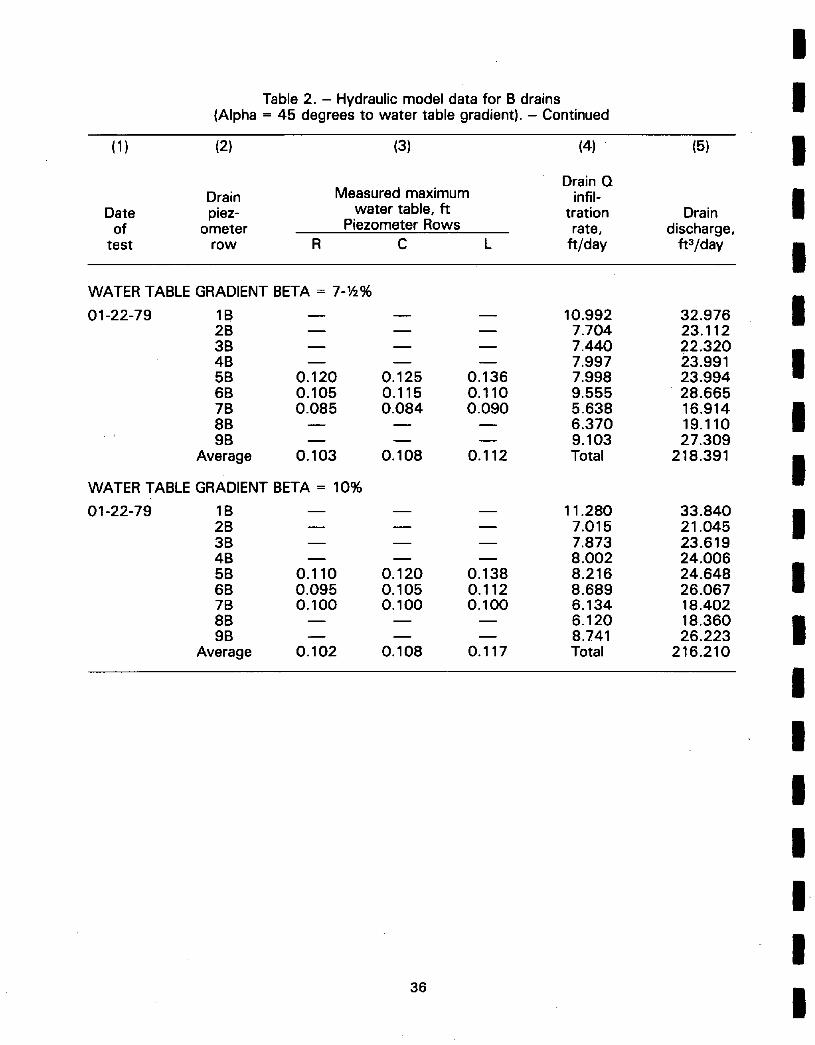
Table 2. - Hydraul ic model data for B drains (Alpha = 45 degrees to wa te r table gradient ) . - Cont inued
( 1 ) (2) (3)
Drain Date piaz-
of ometer test row
(4) (5) i Drain Q
infil- I t ra t ion Drain
rate, discharge, L f t /day f t3/day •
I
Measured max imum wate r table, f t
Piezomater Rows
R C
WATER TABLE GRADIENT BETA = 7 -½%
0 1 - 2 2 - 7 9 1B ~ 2B ~ 3B ~ 4B ~ 5B 0 . 1 2 0 0 .125 6B 0 .105 0 .115 7B 0 . 0 8 5 0 . 0 8 4 8B ~
Average 0 .103 0 .108
WATER TABLE GRADIENT BETA = 10%
0 1 - 2 2 - 7 9
10 .992 3 2 . 9 7 6 7 .704 2 3 . 1 1 2 7 .440 2 2 . 3 2 0 7 .997 23.991
0 .136 7 .998 2 3 . 9 9 4 0 .110 9 .555 2 8 . 6 6 5 0 . 0 9 0 5 . 6 3 8 16 .914
6 . 3 7 0 19 .110 9 .103 2 7 . 3 0 9
0 .112 Total 218 .391
1B B B ~ 11 .280 2B - - o ~ 7 .015 3B ~ ~ B 7 .873 4B - - o ~ 8 . 0 0 2 5B 0 .110 0 . 1 2 0 0 . 1 3 8 8 .216 6B 0 . 0 9 5 0 .105 0 .112 8 . 6 8 9 7B 0 . 1 0 0 0 . 1 0 0 0 . 1 0 0 6 . 1 3 4 8B ~ ~ ~ 6 . 1 2 0 9B B ~ ~ 8.741
Average 0 .102 0 .108 0 .117 Total
3 3 . 8 4 0 2 1 . 0 4 5 2 3 . 6 1 9 2 4 . 0 0 6 2 4 . 6 4 8 2 6 . 0 6 7 18 .402 1 8 . 3 6 0 2 6 . 2 2 3
2 1 6 . 2 1 0
I I I I I I I I
36
I l I I I I

I I I I
Table 3. - Hydraul ic mode l data fo r C dra ins (Alpha = 3 0 deg rees to w a t e r tab le gradient) .
W i d t h o f f lume = 2 . 0 f t ; dep th o f dra ins to barr ier = 2 . 0 f t ; radius o f dra ins + gravel e n v e l o p e = 0 . 0 5 ft ; perpend icu la r drain spac ing = 0 . 7 5 ft ; area con t r ibu t ing to all dra ins = 3 2 . 9 2 ft2; inf i l t rat ion recharge = 8 2 . 1 7 mL /s = 2 5 0 . 7 2 f t3 /day = 7 . 6 1 6 f t /day.
(1) (2) (3) (4) (5)
Drain Q Drain Measu red max imum infil-
Date piez- w a t e r table, f t t ra t ion drain o f o m e t e r P iezomete r R o w s rate, d ischarge,
tes t r o w R C L f t / day f t3 /day
I I I I I I I I I I I I I
W A T E R TABLE GRADIENT BETA = 2 - ½ %
0 1 - 1 8 - 7 9 1C ~ ~ m 1 3 . 4 9 5 4 0 . 4 8 5 2C ~ - - ~ 7.61.1 2 2 . 8 3 3 3C ~ ~ m 8 . 0 6 5 2 4 . 1 9 5 4C ~ ~ ~ 6 . 5 8 9 1 9 . 7 6 7 5C 0 . 0 2 5 0 . 0 2 2 0 . 0 3 3 7 . 8 6 5 2 3 . 5 9 5 6C 0 . 0 4 2 0 . 0 4 8 0 . 0 5 3 5 . 8 2 9 1 7 . 4 8 7 7C 0 . 0 6 0 0 . 0 6 0 0 . 0 5 5 8 . 4 7 6 2 5 . 4 2 8 8C ~ m ~ 7 . 2 7 2 2 1 . 8 1 6 9C ~ ~ ~ 6 . 8 0 9 2 0 . 4 2 7
10C m ~ ~ 6 . 1 8 7 18 .561 A v e r a g e 0 . 0 4 2 0 . 0 4 3 0 . 0 4 7 Total 2 3 4 . 5 9 4
W A T E R TABLE GRADIENT BETA = 5 %
0 1 - 1 8 - 7 9 1C - - m m 1 3 . 4 4 6 4 0 . 3 3 8 2C ~ ~ ~ 8 . 0 3 8 2 4 . 1 1 4 3C ~ m ~ 5 . 3 2 9 1 5 . 9 8 7 4C ~ ~ ~ 7 . 4 5 9 2 2 . 3 7 7 5C 0 . 0 2 0 0 . 0 2 8 0 . 0 3 5 8 . 9 4 4 2 6 . 8 3 2 6C 0 . 0 4 0 0 . 0 4 2 0 . 0 3 8 4 . 9 4 2 1 4 . 8 2 6 7C 0 . 0 5 7 0 . 0 5 3 0 . 0 5 3 9 . 9 2 8 2 9 . 7 8 4 8C m - - ~ 6 . 7 8 0 2 0 . 3 4 0 9C ~ ~ ~ 6 . 3 5 7 2 9 . 0 7 1
10C m ~ ~ 5 . 5 9 4 1 6 . 7 8 2 A v e r a g e 0 . 0 3 9 0 .041 0 . 0 4 2 Total 2 3 0 . 4 5 1
37

Table 3. - Hydraulic model data for C drains (Alpha = 30 degrees to water table gradient). - Continued
( 1 ) ( 2 ) ( 3 ) ( 4 )
Drain Q Drain Measured maximum infil-
Date piez- water table, ft tration of ometer Piezometer Rows rate,
test row R C L f t /day
(5)
Drain discharge,
ft3/day
I I l
WATER TABLE GRADIENT BETA = 7-½%
1C ~ ~ ~ 12.636 2C m ~ ~ 8 .922 3C ~ ~ - - 4.291 4C m ~ ~ 8.199 5C 0.018 0 .025 0 .032 10.171 6C 0 .030 0.031 0 .028 3 .139 7C 0 .045 0 .043 0 .046 9 .323 8C ~ ~ m 9.945 9C ~ ~ ~ 4 .843
10C ~ m - - 2 .792 Average 0.031 0 .033 0 .035 Total
01-19-79
WATER TABLE GRADIENT BETA = 10%
01-19-79 1C 2C 3C 4C 5C 0 .020 6C 0 .032 7C 0 .040 8C 9C
10C Average 0.031
m __ 13.512 ~ 9.894 ~ 5 . 6 8 3
- - ~ 4.041 0 .023 0 .025 12.300 0 .028 0 .028 2 .534 0 .039 0 .052 13 .105
~ 5 .684 ~ 6.655
- - ~ 6 .733 0 .030 0 .035 Total
37 .908 26 .766 12.873 24 .597 30 .513
9.417 27 .969 29 .835 14.529
8 .376 222 .783
40 .536 29 .682 17.049 12.123 36 .900
7 .602 39.315 17.052 19.965 20 .199
240 .423
I i I i I I I I
38
I I I I I I

I I I I
Table-4. - Hydraulic model data for D drains (Alpha = 0 degrees to wa te r table gradient).
Width of flume = 2 .0 ft; depth of drains to barrier = 2 .0 ft; radius of drains + gravel envelope = 0 .05 ft; perpendicular drain spacing = 1.0 ft; area contr ibut ing to all drains = 33 .09 ft2; infi ltration recharge = 46 .92 mL/s = 143.16 ft3/day = 4 .338 f t /day; drain collectors spacing = 3 .0 ft.
(1) (2) ( 3 )
Drain Measured Date piez- maximum
of ometer water table, test r o w f t
(4) (5) (6) (7)
Drain Q infil- Drain
Drain trat ion Drain total collector rate, discharge, discharge, number f-t/day ft3/day ft3/day
I I I I I I I I I I I I I
WATER TABLE GRADIENT BETA = 21/2%
01-17-79 2D-1 0 .045 2D-2 0 .068 2D-3 0 .072 2D-4 0 .083 2D-5 O. 100 2D-6 0.113
Average 0 .080
01-12-79 3D-1 0 .026 & 3D-2 0 .042
01-15-79 3D-3 0 .059 3D-4 0 .070 3D-5 0 .080 3D-6 0 .098
Average 0 . 0 6 3
WATER TABLE GRADIENT BETA = 5%
01-17-79 2D-1. 2D-2 2D-3 2D-4 2D-5 2D-6
Average
0!-12-7.9 3D-1 & 3D-2
01-15-79 3D-3 3D-4 3D-5 3D-6
• . Average
0 .080 0 .095 0 .090 0 .099 0 .100 0 .098 0 .063
0 .015 ; 0 . 030 • 0 .065
0 . 0 7 0 0 .085 0 .105 0 .062
1D 1.374 8 .244 - 2D 2 .906 17.436 - 3D 3 .769 22 .614 - 4D 3 .945 23 .670 - 5D 5.157 30 .942 102.906 End - 3 0 . 2 0 4 -
Total 133.110 -
1D 3 .240 19.440 - 2D 3 .678 22 ,068 - 3D 2 .626 15.756 - 4D 4 . 2 2 0 2 5 . 3 2 0 - 5D 4 .680 2 8 , 0 8 0 110.664 End - 23 .677 -
Total 134.341 -
1D 2 ,366 14.196' - 2D 2 .293 13.758 - 3D 2 .877 17.262 - 4D 2 .945 17.670 - 5D 5 .805 3 4 . 8 3 0 97.716 End - 33 .208 -
Total 130 .924 -
1D 2 .379 14.274 - 2D 3 .192 19.152 - 3D 2 .374 14,244 - 4D 4 .107 24 .642 - 5D 5 .599 3 3 . 5 9 4 105.906 End - 3 4 . 4 9 2 -
Total 140.398 -
39

(1) (2)
Table 4. - Hydraulic model data for D drains (Alpha = 0 degrees to water table gradient). - Continued
(3) (4) (5) (6) (7)
I I I
Drain Date piez-
of ometer test row
Drain Q Measured infil- Drain maximum Drain tration Drain total
water table, collector rate, discharge, discharge, ft number ft/day ft3/day ft3/day
WATER TABLE GRADIENT BETA = 7½%
01-17-79 2D-1 0.099 1D 2D-2 0.115 2D 2D-3 0.110 3D 2D-4 0.109 4D 2D-5 O. 110 5D 2D-6 0.098 End
Average 0.107 /
01-12-79 3D-1 0.004 1D & 3D-2 0.014 2D
01-15-79 3D-3 0.035 3D 3D-4 0.060 4D 3D-5 0.076 5D 3D-6 O. 115 End
Average 0.051
WATER TABLE GRADIENT BETA = 10%
01-17-79 2D-1 0.097 1D 2D-2 0.113 2D 2D-3 O. 107 3D 2D-4 0.108 4D 2D-5 0.097 5D 2D-6 0.094 End
Average O. 103
01-12-79 3D-1 -0 .038 1D & 3D-2 -0.015 2D
01-15-79 3D-3 0.026 3D 3D-4 0.068 4D 3D-5 O. 102 5D 3D-6 0.141 End
Average 0.047
2.682 2.315 2.391 2.445 5.884
Total
1.508 2.266 2.049 3.978 6.324
Total
2.534 2.026 2.119 1.891 6.090
D
Total
1.305 2.270 2.062 3.437 7.006
Total
16.092 13.890 14.346 14.670 35.304 41.308
135.610
9.048 13.596 12.294 23.868 37.944 40.560
137.310
15.204 12.156 12.714 11.346 36.540 52.391
140.351
7.830 13.620
•12.372 20.622 42.036 53.510
149.990
m
m
m
D
94.302
96.750
87.960
96.480
I I I I I I I
i i
4 0
I I I I

Table 5. - Hydraulic model data, infiltration recharge • , . . . I
compared w=th dram d~scharge for all dram sets and all flume slopes.
I I I
( 1 ) (2) (3) (4) (5) Total Infiltration
Water infil- Total minus table Date tration drain drain
gradient, of recharge, discharge, discharge, % test ft3/day ft3/day ft3/day
I II I I I I I I I I I
A DRAINS (ALPHA = 90 DEGREES TO WATER TABLE GRADIENT)
0 01-30-79 188.56 160.86 US End 31.66
Total 192.52 2 ½ 01-30-79 188.56 189.90 5 01-30-79 188.56 169.71 7 ½ 01-30-79 188.56 176.90
10 01-30-79 188.56 176.75
B DRAINS (ALPHA = 45 DEGREES TO WATER TABLE GRADIENT)
2½ 01-22-79 219.69 217.45 5 01-22-79 219.69 218.98 71/= 01-23-79 219.69 218.39
10 01-23-79 219.69 216.21
C DRAINS (ALPHA = 30 DEGREES TO WATER TABLE GRADIENT)
2½ 01-18-79 250.72 234.59 5 01-18-79 250.72 230.45 7½ 01-19-79 250.72 222.78
10 01-19-79 250.72 240.42
D DRAINS (ALPHA = 0 DEGREES TO WATER TABLE GRADIENT)
2½ 01-17-79 143.16 102.91 End 30.21
Total 133.1 £ 5 01-17-79 143.16 97.72
End 33.21 Total 130.92
71/= 01-17-79 143.16 94.30 End 41.31
Total 135.61 10 01-17-79 143.16 87.96
End 52.39 Total 140.35
-3 .96 -1 .34 18.85 11.56 11.81
2.24 0.71 1.30 3.48
16.13 20.27 27.94 10.30
40.25 m
45.44
48.86
55.20
I I I
41

Table 6. - Hydraulic model data and data computed using programs EJC20M and EJC16M. Maximum water table heights between
adjacent drains for all drain sets and ,all flume slopes.
Width of flume = 2.0 ft; depth of drains to barrier = 2.0 ft; radius of drains + gravel envelope = 0.05 ft.
A DRAINS (ALPHA = 90 DEGREES TO WATER TABLE GRADIENT)
I I I I
Perpendicular drain spacing = 1.50 ft; area contributing to all drains = 24.75 ft2; infiltration recharge = 61.8 mL/s = 188.56 ft3/day = 7.619 if/day. Computed permeability = 38.02 if/day, based on measured average maximum water table height for A drains at water table gradient Beta = 0% on 02-26-79, using program EJC2OM. Computed water table heights based on program EJC 16M.
( 1 ) (2) (3) (4) Water Measured Computed table Date maximum maximum
gradient of water table, water table, % test ft ft
2½ 01-30-79 0.171 0.164
I I I I
5 01-30-79 O. 155 0.164 7½ 01-30-79 O. 153 O. 164
10 01-30-79 O. 144 O. 164
(1) (2) (3) (4)
Measured maximum Computed Water table Date water table, ft maximum
gradient, of Piezometer Rows water table, % test R C L ft
B DRAINS (ALPHA = 45 DEGREES TO WATER TABLE GRADIENT)
Perpendicular drain spacing = 1.06 ft; area contributing to all drains = 29.24 ft=; infiltration recharge = 72 mL/s = 219.69 ft3/day = 7.513 h/day.
2½ O1-22-79 0.097 O.109 O.115 0.103 5 01-22-79 0.098 0.106 0 .113 0.103 7½ 01-23-79 0.103 0.108 0.112 0.103
10 01-23-79 0.102 0.108 0.117 0 .103
42
I I I i I I

Table 6. - Hydraulic model data and data computed using programs EJC20M and EJC16M. Maximum water table heights between
adjacent drains for all drain sets and all flume slopes. - Continued
(1) (2) (3) (4)
Measured maximum Computed Water table Date water table, ft maximum
gradient, of Piezometer Rows water table, % test R C L ft
I I I I I I I I I I I I i I
C DRAINS (ALPHA = 30 DEGREES TO WATER TABLE GRADIENT)
Perpendicular drain spacing = 0.75 ft; area contributing to all drains = 32.92 ft2; infiltration recharge = 82.17 mL/s = 250.72 ft3/day -- 7.616 ft/day.
2½ 01-18-79 0.042 ~..043 0.047 0.064 5 01-18-79 0.039 0.041 0.042 0.064 71/z 01-19-79 0.031 0.033 0.035 0.064
10 01-19-79 0.031 0.030 0.035 0.064
43

Table 6. - Hydraulic model data and data compared using programs EJC20M and EJC16M. Maximum water table heights
between adjacent drains for all drain sets and all flume slopes. - Continued
(1) (2) (3) (4) (5)
I I I
water Drain Measured Computed table Date piez- maximum maximum
gradient of ometer water table, water table, % test row ft ft
D DRAINS (ALPHA = 0 DEGREES TO WATER TABLEGRADIENT)
Perpendicular spacing = 1.0 ft; area contributing to all drains = 33.09 ft2; infiltration recharge = 4.92 mL/s = 143.16 ft3/dy = 4.338 f-t/day; drain collector spacing = 3.0 ft.
2 1 / 2 01-17-79 2D 0.080 0.059 2V2 01-12-79 3D 0.063 0.059
& 01-15-79
5 01-17-79 2D 0.094 0.059 5 01-12-79 3D '0.062 0.059
& 01-15-79
71 /2 01-17-79 2D 0.107 0.059 71 /2 01-12-79 3D 0.051 0.059
& 01-15-79
10 01-17-79 2D 0.059 0.059 10 01-12-79 3D 0.059 0.059
& 01-15-79
I I I I I I I
44
G P O 8 B S - t 3 2
I I I I I I I

I I I I I I I I I I I I I I I I I I
Mission of the Bureau of Reclamation
The Bureau of Reclamation of the U.S. Department of the Interior is responsible for the development and conservation of the Nation's :water resources in the Western United States.
The Bureau's original purpose "to provide for the reclamation of arid and semiarid/ands in the West" today Covers a wide range of interre- lated functions. These include providing municipal and industrial water supplies; hydroelectric power generation;.irrigation water for agricul- ture; water quality improvement; flood control; river navigation, river regulation and control; fish and wildlife enhancement; outdoor recrea- tion; and research on water-related design, construction, materials, atmospheric management, and wind and solar power.
Bureau programs most frequently are the result of close cooperation with the U.S. Congress, other Federal agencies, States, local govern- ments, academic institutions, water-user organizations, and other concerned groups.
A free pamphlet is available from the Bureau entitled "Publications for Sale." It describes some of the technical publications currently available, their cost, and how to order them. The pamphlet can be obtained upon request from the Bureau of Reclamation, Attn D-922, P O Box 25007, Denver Federal Center, Denver CO 80225-0007.