DRAFT - University of Michigan

DRAFTJune, 2002

EVALUATION OF OBSERVATION-BASED METHODS FOR ANALYZINGOZONE PRODUCTION AND OZONE-NOX-VOC SENSITIVITY

by

Sanford SillmanDepartment of Atmospheric, Oceanic and Space Sciences

University of MichiganAnn Arbor, Michigan 48109-2143

Purchase Order number 1D-5795-NTEX

Project Officer

Deborah Luecken_______________________________

Atmospheric Research and Exposure Assessment LaboratoryResearch Triangle Park, NC 27711

NATIONAL EXPOSURE RESEARCH LABORATORYOFFICE OF RESEARCH AND DEVELOPMENT

U.S. ENVIRONMENTAL PROTECTION AGENCYRESEARCH TRIANGLE PARK, NC 27711

2

TABLE OF CONTENTS

Section page

Notation.

Acknowledgements

EXECUTIVE SUMMARY

1. INTRODUCTION

1.1 Overview

1.2 Scope of this report

1.3 The purpose of OBMs

1.4 VOC versus NOx as the major source of uncertainty

1.5 Background information on O3-NOx-VOC sensitivity

2. SURVEY OF OBSERVATION-BASED METHODS

2.1 Criteria for Evaluation

2.2 Overview of OBM approaches and issues

2.3 Evaluation of individual OBMs

2.3.1 Secondary species as NOx-VOC indicators

2.3.2 Smog production algorithms

2.3.3 Constrained steady state – instantaneous chemistry based on measured NOx and VOC

2.3.4 Observation-based model using measured NOx and VOC (Cardelino-Chameides)

2.3.5. Direct analysis of measured NOx and VOC to estimate emissions

2.3.6 Inverse modeling for NOx and VOC emissions

2.3.7. Empirical ozone isopleths

2.3.8 Other methods

2.4 Supplemental topic: Receptor modeling

2.5 Supplemental topic: Evaluating long term trends for ozone and related air pollutants

2.6 Conclusions

3. THEORETICAL EVALUATION

3

3.1 NOx-VOC indicators

3.1.1 Summary information

3.1.2 Conclusions and recommendations

3.1.3 Results from 3-d models

3.1.4 Results from 0-d calculations and isopleth plots

3.1.5 Contrary evidence

3.1.6 Model correlations between indicator species

3.1.7 Results from ambient measurements

3.1.8. Model evaluations with measured indicator species: a method for regulatory use

3.1.9 Results for O3 versus PAN: possible impact of erroneous measurements

3.1.10 Supplementary topic: Definition of O3-NOx-VOC sensitivity.

3.1.11 Supplementary topic: Determining background values

3.1.12 Supplementary topic: radical chemistry and O3-NOx-VOC sensitivity

3.2 SMOG PRODUCTION ALGORITHMS (EXTENT-OF-REACTION PARAMETERS)



3.2.3 The smog production concept: results from smog chamber experiments

3.2.4 Evaluation with 3-d models

3.2.5 Contrary evidence

3.2.6 Uncertainties associated with the theoretical basis

3.2.7. Applications of smog production algorithms

3.2.8 Evaluations with ambient measurements

3.3 CONSTRAINED STEADY STATE AND OTHER ANALYSES BASED ON AMBIENT VOC AND NOx



3.3.3 Constrained steady state models

3.3.4 Short formulas for NOx-VOC sensitivity

4

3.3.5 Integrating from instantaneous ozone production to ozone concentrations

3.3.6 Accuracy and completeness of NOx and VOC measurements

3.3.7 Methods for evaluating emission inventories from measurements

3.3.8 Inverse modeling

3.3.9 Other uncertainties

4.0 PRACTICAL IMPLEMENTATION OF OBSERVATION-BASED METHODS


4.1.1 Required measurements

4.1.2 Quality assurance of measurements

4.1.3 Interpretation of measurements

4.1.4 Evaluation of air quality models

4.1.5. Summary of proposed regulatory procedure

4.2 Constrained steady state models with measured NOx and VOC

4.2.1 Required measurements

4.2.2 Quality assurance of measurements

4.2.3 Interpretation of measurements

4.2.4 Evaluation of air quality models

4.2.5 Summary of proposed regulatory procedure

5. RECOMMENDATIONS FOR FUTURE RESEARCH


5.2 Constrained steady state/measured NOx and VOC

6. REFERENCES

APPENDIX: ADDITIONAL RESULTS FOR NOx–VOC INDICATORS

5

NOTATION

AQM Three-dimensional Eulerian air quality model (e.g. UAM, RADM, etc.)

CB-IV The Carbon Bond IV photochemical mechanism (Gery et al., 1989).

CSS Constrained steady state model (Kleinman et al., 1997). This term is also used to refer to theobservation-based model developed by Cardelino and Chameides (1995).

Hx (radicals, odd hydrogen): The sum of OH, HO2 and RO2 and RCO3 radicals (analogous to CH3O2 andCH3CO3).

kOHi Rate constant for the reaction of OH with and individual VOC (VOCi).

LH Summed loss rate for NOx, including conversion to nitric acid and organic nitrates.

LN Summed rate of photochemical removal of NOx, also equal to the rate of production of NOz.

NOx(i) Initial NOx concentration in smog chamber experiments

NOy Total reactive nitrogen, including NOx, HNO3, NO3- and organic nitrates.

NOz NOx reaction products, or NOy-NOx.

O3b, NOyb, etc: Background (upwind) values of O3, NOy, etc.

OBM Observation-based method for determining O3-NOx-VOC sensitivity. The observation-basedmodel developed by Cardelino and Chameides (1995), sometimes referred to as OBM, is referredto here as CSS.

OPEN Ozone production efficiency per NOx.

OPER Ozone production efficiency per primary radical production.

PO3 Rate of production of ozone.

PHNO3 Rate of production of nitric acid.

PorgN Rate of production of organic nitrates (including PAN).

Pperox Rate of production of peroxides (including H2O2 and organic peroxides).

ppb parts per billion by volume

ppm parts per million by volume

ppt parts per trillion by volume

Q Summed source of odd hydrogen radicals, including OH, HO2 and RO2 (referred to as Q inKleinman et al., 1997), also referred to as SH.

6

RADM Regional Acid Deposition Model and associated photochemical mechanism (Stockwell et al.,1990).

ROOH Organic peroxides

rVOC Reactivity-weighted sum of VOC, equal to kOHiiÂ VOCi

SH Summed source of odd hydrogen radicals, including OH, HO2 and RO2 (referred to as Q inKleinman et al., 1997).

SN Summed source of NOx.

SP Smog produced (in association with smog production algorithms)

SPmax Maximum potential smog production for a given precursor mixture (in association with smogproduction algorithms).

VOC Summed volatile organic compounds

VOCi Concentration of an individual VOC

7

ACKNOWLEDGEMENTS

This work was supported by the Office of Research and Development of the U.S. Environmental Protection

Agency under grant #F005300. Many of the results reported here were based on research supported by the Office

of Research and Development of the U.S. Environmental Protection Agency under the Science To Improve Results

(STAR) program, grant #R826765, and in association with the Southern Oxidant Study. Although the research

described in this article has been funded by EPA, it has not been subjected to peer and administrative review by

either agency, and therefore may not necessarily reflect the views of the agency, and no official endorsement should

be inferred.

8

EXECUTIVE SUMMARY

Observation-based methods (OBMs) refer to techniques for using ambient measurements to evaluate the

sensitivity of ozone to emissions of anthropogenic NOx and volatile organic compounds (VOC). As such, they

represent part of a trend to link the predictions of air quality models more closely to ambient measurements. OBMs

offer several advantages as a basis for establishing and evaluating regulatory policy. These include:

• Measurement-based evaluation of the accuracy of model predictions concerning the effectiveness of

control strategies, especially with regard to the issue of NOx versus VOC controls.

• Evaluation of the accuracy of emission inventories, which represent a major source of uncertainty in air

quality models.

• Evaluation of the effectiveness of previously implemented control strategies, and identification of the

reasons for success or failure of existing regulatory polices – thus providing a basis for accountability

for control policy.

The major OBMs require measurements for the following species: O3, total reactive nitrogen (NOy), NOx, and

speciated VOC. Use of OBMs would require an extensive network of measurements for these species with high

standards for accuracy. If implemented, OBMs would correct a long-standing tendency to evaluate air quality

models based only on their ability to reproduce observed ozone. It has been recognized since at least 1991 that

comparisons with measured ozone are not sufficient to insure the accuracy of control strategy predictions from air

quality models (NRC, 1991). The OBMs can provide a much stronger measurement-based evaluation of model

accuracy.

The main focus of OBMs has been the issue of NOx versus VOC controls for ozone, although the same

techniques can provide insight for other ozone-related issues as well. O3-NOx-VOC sensitivity represents one of the

largest uncertainties associated with the process of ozone formation, and is also a major uncertainty in terms of

regulatory policy. It is generally known that for some conditions, the rate of ozone formation increases with

increasing NOx and is largely insensitive to anthropogenic VOC, while for other conditions, ozone formation

increases with increasing VOC and is insensitive (or negatively sensitive) to NOx. However, it is difficult to

determine whether ozone in an individual location or during a specific event is primarily sensitive to NOx or VOC.

9

The NOx-VOC issue is a major source of uncertainty associated with predictions for the effectiveness of control

strategies for air pollutants.

OBMs were originally conceived as a replacement for the 3-dimensional Eulerian air quality models (AQMs),

which are regularly used to establish and evaluate regulatory policy. The OBMs were intended to provide the same

level of analysis as the AQMs, but would derive their initial concentration fields from ambient measurements rather

than from emission inventories. It is now recognized that OBMs have their own uncertainties and limitations and

are unlikely to provide a replacement for AQMs. However the OBMs are potentially very useful as a complement

to AQMs. OBMs provide a link between AQMs and ambient measurements, which is often missing in regulatory

studies, and provide a basis for evaluating the accuracy of model control strategy predictions. OBMs are also useful

as stand-alone methods (if their limitations are properly recognized) because they can provide an analysis of trends

over an entire season, and can identify event-to-event variations that might be overlooked by the AQMs.

Two OBMs are especially worthy of investigation: (i) the method of NOx-VOC indicators, which uses total

reactive nitrogen (NOy), NOx reaction products (NOz), and nitric acid to derive inferences about O3-NOx-VOC

sensitivity; and (ii) constrained steady state calculations that use ambient VOC and NOx. These two methods are

complementary, in that they use different measurements to draw inferences about the same issue. The constrained

steady state method can also be combined with other analytical tools (e.g. from Parrish et al., 1998) that use

measured NOx and VOC to evaluate the accuracy of emission inventories. Analyses that show consistent results

from AQMs, NOx-VOC indicators and measured NOx and VOC are very likely to provide accurate predictions

concerning O3-NOx-VOC sensitivity.

NOx-VOC indicators are based on the theory that the ratios O3/NOy, O3/NOz and O3/HNO3, and the equivalent

species correlations between species, show different values depending on whether ozone is predominantly sensitive

to NOx or VOC. This approach is based on results from 3-d Eulerian air quality models, which generally show that

high values of these ratios are associated with NOx-sensitive chemistry and low values are associated with VOC-

sensitive chemistry. Some contradictory results from models have been reported, but these can be corrected by

adjusting the original indicator ratios to account for upwind conditions. The ratio of ozone production per NOx

removed (also referred to as ozone production efficiency per NOx) is also higher in model calculations for NOx-

sensitive conditions then for VOC-sensitive conditions. The ratio H2O2/HNO3 is strongly associated with NOx-

10

VOC sensitivity, but this ratio is more difficult to use in practice because measured H2O2 or total peroxides are

usually not available.

There is strong evidence from both models and ambient measurements that indicator ratios show different values

for NOx-sensitive versus VOC-sensitive conditions. However, there is no strong evidence that indicator ratios are

universally applicable for all ambient conditions. Therefore, ambient values of indicator ratios should be viewed as

a broad indication of NOx-VOC sensitivity patterns, rather than as a rigid “rule of thumb”. Indicator ratios are

likely to be useful for identifying apparently different NOx-VOC conditions between different locations or for

different events. In addition, indicator ratios and species correlations are especially useful as a method for

evaluating the accuracy of NOx-VOC predictions from AQMs. When predicted correlations between O3 and NOy

and between similar species are compared with measured values, patterns often emerge that can be interpreted as

evidence of bias in the AQM towards VOC-sensitive or NOx-sensitive chemistry. These interpretations are likely

to remain valid even if the stated connection between indicator ratios and O3-NOx-VOC sensitivity is not precise.

Changes in the observed correlations between O3 and NOy can also be used to identify the causes of changes in

O3 over time, as a basis for evaluating the effectiveness of control strategies. The correlation between O3 and NOy

can also be used to identify changes in global background O3 and its impact on O3 in the U.S.

Constrained steady state calculations are based on the theory that O3-NOx-VOC sensitivity is closely connected

to ambient concentrations of VOC and NOx. Ozone-precursor sensitivity is often not directly linked to VOC/NOx

ratios, because ozone is the result of photochemical production over several hours and along extended air mass

trajectories. Photochemistry along these trajectories is affected by short-lived VOC species, including biogenic

species, that my not be leave evidence as the air mass moves downwind. However, the instantaneous rate of ozone

production shows a NOx-VOC sensitivity pattern that is closely associated with ambient NOx and VOC. The NOx-

VOC sensitivity for instantaneous ozone production is also loosely associated with the ratio of reactivity-weighted

VOC (rVOC) to NOx.

The constrained steady state models calculate instantaneous rates of ozone production as a function of ambient

NOx and VOC (and, if available, incident solar radiation). The version developed by Cardelino and Chameides

(1995) also calculates the sum of instantaneous ozone production rates and summed sensitivity to NOx and VOC,

assuming that a series of measurement sites can be used to characterize photochemistry in an urban area. This

11

analysis of summed ozone production is likely to be closely related to O3-NOx-VOC sensitivity, but results may

vary depending on the exact location of measurement sites and transport patterns. As is the case for NOx-VOC

indicators, the constrained steady state calculations are useful for providing a general indication of O3-NOx-VOC

sensitivity in a specified region.

Measured NOx and VOC can also be used directly to infer emission rates of NOx and VOC and to evaluate

emission inventories. This is important because emission inventories represent the largest uncertainty in air quality

models and are often the major source of uncertainty in NOx-VOC predictions from models. Parrish et al. (1998)

described a series of correlations between individual VOC that can be used to infer emission rates. The same

correlations can be used to evaluate the accuracy of VOC and NOx in air quality models. As is the case for NOx-

VOC indicators, comparison of results from AQMs with measured NOx and VOC can be used to identify biases in

AQMs that affect NOx-VOC predictions. The same analysis can also be used to identify changes in emissions of

NOx and VOC over time.

Smog production algorithms, which are widely used to evaluate O3-NOx-VOC sensitivity in regulatory

applications, are also evaluated in this document. Smog production algorithms also use measured total reactive

nitrogen (NOy) to infer NOx-VOC sensitivity, but (in contrast to the indicator method) the interpretation of

measurements is based primarily on results from smog chamber experiments rather than from 3-d air quality models.

The smog production algorithms are also based on the theory (derived from both smog chamber experiments and 0-d

calculations) that VOC-sensitive conditions are associated with relatively fresh emissions and NOx-sensitive

conditions are associated with photochemically aged air in which most of the NOx has reacted to form O3. The

smog production algorithms assume that in photochemically aged air the summed amount of ozone produced per

NOx (ozone production efficiency) has a constant value that is independent of VOC emissions. Evidence from both

0-d calculations and ambient measurements challenges this view. Results from 3-d models suggest that the smog

production algorithms can identify locations with strongly VOC-sensitive chemistry, which are usually associated

with unprocessed direct emissions. The smog production algorithms are less reliable for photochemically aged air,

which usually has the highest O3 and which can have either NOx-sensitive or VOC-sensitive conditions.

Use of OBMs (including indicator ratios, constrained steady state calculations and direct inferences from

measured NOx and VOC) depends critically on the availability and accuracy of measurements. The NOx-VOC

12

indicators require a network of measured O3 and either NOy or HNO3 (and, if possible, NOx) over a region that

includes locations with the highest O3. Constrained steady state and related methods require measurements of a

relatively complete set of primary VOC, including short-lived and biogenic species, and also measured NOx. These

methods do not require as extensive a measurement network as the NOx-VOC indicators do, but the measurements

must be extensive enough to characterize VOC and NOx throughout a metropolitan region and to include locations

with high biogenic VOC. In both cases it is critically important that measurements meet standards of accuracy.

Measurement techniques for NOx and NOy are both subject to characteristic errors that would compromise their use

in evaluations of O3-NOx-VOC sensitivity. Questions have also been raised about the accuracy of measured VOC,

especially about measurements of highly reactive species. In general, it is preferable to base the OBMs with a

relatively small number of highly accurate measurements, rather than an extensive network of measurements of

questionable accuracy.

Because accuracy of measurements is a critical issue, analysis with an OBM should include evaluation of the

pattern of measured data to identify possible sources of error. The species correlations associated with NOx-VOC

indicators and correlations among VOC used to evaluate emissions can also be used to identify possible errors in

measured data sets and to identify other ambient conditions that would invalidate results from an OBM.

Finally, standard protocols should be developed for the use of OBMs in regulatory applications. These protocols

would facilitate the interpretation of results from investigations in different locations and insure that quality

assurance of measurements is included. Protocol for NOx-VOC indicators should include display of arrays of

measured correlations between O3 and NOy, etc., in comparison with model patterns that would identify

characteristic errors in measurements or other inconsistencies that would invalidate the method. Protocol for NOx-

VOC indicators should also include guidance for comparison between measured indicator correlations and results of

an AQM, and development of standards that would define a successful model-measurement comparison. Protocol

for constrained steady state should include display of measured correlations between individual VOC, following

methods from Parrish et al. (1998) that would identify erroneous measurements or missing VOC. This would also

provide an evaluation of the emission inventory to be used in an AQM. Protocol would also need to be established

for situations in which analyses from OBMs and from standard air quality models gave contradictory results.

13

SECTION 1. INTRODUCTION

1.1 OVERVIEW

Observation-based methods (OBMs) refer to a collection of techniques that have been developed for analyzing

the ozone production process directly from ambient measurements. The OBMs have been proposed as methods that

can be used in the development of control strategies for reducing the levels of ambient ozone during pollution

events. Specifically, OBMs have been proposed as methods to evaluate the relative effectiveness of controls on

volatile organic compounds (VOC) as opposed to controls on nitrogen oxides (NOx) as strategies for reducing

ambient ozone.

Traditionally, analysis of ozone production and the development of control strategies have been based on 3-

dimensional air quality models (AQMs). These AQMs include the following components: an inventory of

anthropogenic and biogenic emissions; a representation of meteorology during the event or events of interest; a

mechanism representing photochemical reactions believed to be important in ozone formation; and a simulation

procedure within a 3-dimensional grid that represents the process of emissions, photochemical transformations, and

transport.

The AQMs have a number of advantages as a basis for developing ozone policy. They provide an analysis of

specific air pollution events that includes the most complete available knowledge of the ozone formation process.

Computer simulations are by their nature flexible and can be adopted to represent conditions unique to individual

locations. They also can be modified to reflect scientific advances. They are especially advantageous for the

policy-making process because they can analyze the impact of specific emission sources (by location or by source

type) and evaluate the impact of specific proposed policies on ambient ozone. No OBM can evaluate the impact of

specific emission sources or control policies in this level of detail.

While the AQM's have been successful in providing specific answers to the problem of ozone control strategies,

it has been more difficult to establish whether those answers are accurate. As computer models, AQMs are

dependent on a range of inputs and assumptions concerning the process of ozone formation. These assumptions

affect not just the model ability to successfully model the amount of ozone formed in the atmosphere, but also the

14

ability to predict the impact of control strategies. Specifically, results from AQM's depend on the accuracy of

emission inventories, which have been regarded as very uncertain (e.g. Fujita et al., 1992; Geron et al., 1994).

Evaluation of the accuracy of predicted control strategies from AQMs has also been unsatisfactory. The

performance of AQMs has been evaluated extensively versus ambient ozone, and statistical criteria have been

established to define an acceptable level of performance (NRC, 1991). However, model accuracy for ozone by

itself does not guarantee the accuracy of model predictions for the effectiveness of control strategies. It is frequently

possible to generate alternative model scenarios for the same event, with similar O3 but different predictions for the

impacts of VOC and NOx controls on O3 (e.g. Sillman et al., 1995; Pierce et al, 1998). Specific AQM applications

have occasionally been evaluated against a more extensive array of ambient measurements (e.g. Jacobson et al.,

1996) but it is difficult to establish whether control strategy predictions from AQMs are accurate.

Uncertainties associated with isoprene (C5H8), a biogenic VOC emitted primarily by deciduous trees, have been

a major source of dissatisfaction with AQM's. It is now recognized that isoprene has a significant impact on ozone

formation in many urban areas in the U.S. AQMs that include isoprene often give results for the effectiveness of

NOx-based and VOC-based control strategies that are very different from AQMs without isoprene or with isoprene

from different emission inventories (Pierce et al., 1998). The initial recommendations to develop observation-

based approaches for ozone was motivated largely by the uncertainty associated with isoprene (Chameides et al.,

1992). For many years AQMs were used without including biogenic VOCs, and errors resulting from these

omissions were not identified by the evaluation procedures of AQM's. This might be counted as a failure of AQMs

as an analytical tool.

OBMs offer several general advantages over AQMs for analyzing ozone. Unlike the AQMs, the proposed

OBMs are usually not dependent on the accuracy of emission inventories. Since these inventories are believed to be

the major source of uncertainty in AQMs, methods that do not require the use of these inventories may have

significantly less uncertainty. OBMs are generally perceived as less dependent on model assumptions than AQMs.

OBMs are also advantageous because they have a direct link to ambient measurements. Because they rely on

measurements, OBM predictions are based on real-world conditions to a greater extent than AQMs. By relying on

measurements, the OBMs also may provide stronger evidence in support of their control strategy predictions.

Perhaps the most useful aspect of OBMs is their ability to compensate for the drawbacks of AQMs. When OBMs

15

are used in combination with standard AQMs, they provide a link between AQM predictions and ambient

measurements that is often missing in the standard AQM analysis.

While OBMs offer advantages as an analytical tool, there are also major disadvantages and potential sources of

error associated with OBMs. These sources of error are especially important because the disadvantages of OBMs

are not known as widely as the sources of error in standard AQMs. Like AQMs, the OBMs are always dependent on

a series of assumptions about the ozone formation process. Accuracy of measurements and the spatial

representativeness of the measurement network are also potential errors for OBMs.

1.2 SCOPE OF THIS REPORT

This report provides a critical evaluation of the various proposed OBMs, as part of an effort to develop guidance

for the use of OBMs in air quality management. It includes OBMs that can be used to analyze ozone production

during air pollution events in specific urban areas, usually in terms VOC-NOx sensitivity. The report also includes

methods that use observations to evaluate and correct emission inventories. These methods are included only if they

are useful for analyzing ozone production during individual events in specific locations.

A number of issues peripherally related to the process of ozone production are specifically excluded from this

analysis. The development and evaluation of photochemical mechanisms (usually involving smog chamber or

chemical kinetics experiments) is clearly observation-based, but this represents a separate issue and is not included

in this report. The development of meteorological fields for use in air quality models is also excluded. Receptor

modeling, analysis of ozone incremental reactivity for individual VOC and evaluation of ozone production

efficiency per NOx are discussed briefly, but are mainly beyond the scope of this report. This report focuses

exclusively on physical processes and does not consider economics or cost-benefit analysis.

Section 2 presents a survey of the various OBMs. It includes a description of each OBM, the rationale for its use,

the extent of investigations designed to demonstrate its validity, and evaluates practical strengths and weaknesses of

the method. Based on this survey, three or four of the most promising OBM techniques will be selected for more

detailed investigation.

Sections 3 and 4 provide an in-depth investigation of the selected OBMs, including the theoretical basis,

justification, and weaknesses of the method (Section 3) and the practical issues of implementation for air quality

16

management (Section 4). The latter includes a discussion of the issues that need to be resolved for the use of OBMs

in combination with standard AQMs.

If OBM's are to be used widely as a tool for air quality management, protocol will need to be developed for

interpreting specific applications. This should include evaluation of the quality of measurements that drive the

OBM and tests for the validity of the OBM in the individual application. In addition, protocol must be developed to

reconcile cases in which analysis based on OBMs disagree with the results of standard air quality models. These

issues will be addressed discussed in Section 4.

1.3 THE PURPOSE OF OBMs

Observations are routinely used throughout the atmospheric sciences, e.g. to evaluate atmospheric models and to

derive inferences about various atmospheric processes. In this report the concept of observation-based methods is

linked to one specific purpose: evaluation of whether ozone formation rates are sensitive primarily to VOC or to

NOx. Only OBMs that address this specific issue are included. Some OBMs that address some secondary issues

that directly relate to the VOC-vs.-NOx issue (e.g. accuracy of emission inventories) are also included.

The VOC-NOx issue is the focus of OBMs because it represents the major source of uncertainty in the evaluation

of control strategies for ozone (see next section). Predictions about control strategies are all subject to uncertainties

based on model formulation, imprecise knowledge of ambient conditions and uncertain identification of atmospheric

sources. The issue of VOC-NOx chemistry typically leads to uncertainties that are much larger than the other issues.

Erroneous representation of VOC-NOx chemistry can lead models to predict that a particular strategy will be highly

effective in lowering ambient ozone, when in fact the recommended strategy would have no impact on ambient

ozone or would cause ozone to increase. This report evaluates OBMs that are designed specifically to reduce the

uncertainty associated with VOC-NOx sensitivity.

This report includes some OBMs that are designed to address a secondary goal: the evaluation of the accuracy of

emission inventories. Evaluation of emission inventories is included because this often represents the main source

of uncertainty in VOC-NOx predictions from AQMs. Some of the proposed OBMs seek to duplicate the analysis of

transport and photochemistry contained in standard AQM's, while eliminating the need for an emission inventory.

Methods that seek to adjust emission inventories in AQMs based on observations are closely related to these OBMs,

and are therefore included for comparison.

17

The concept of OBMs often includes methods that can be used to evaluate the accuracy of control strategy

predictions from AQMs. This type of model evaluation should also be recognized as part of the purpose of OBMs.

Methods of model evaluation are not included explicitly in this report, but are included the discussion of combined

approaches with OBMs and AQMs (Section 4.)

The techniques of receptor modeling (Henry, 1984) should also be recognized as an observation-based approach

with many similarities to the methods considered here. Receptor modeling also seeks to derive information about

pollutants directly from observations. Typically, receptor techniques involve observation-based signals for specific

pollutant sources. These techniques are included in the survey of observation-based approaches (Section 2) but have

not been included in the in-depth analysis (Section 3 and 4) because they address a somewhat different issue.

Investigation of ozone trends and evaluation of the successes and/or failures of past regulatory policy have

become an increasingly important component of air quality analyses. These investigations are also closely linked to

observations and use observation-based approaches. Many of the OBMs proposed for use to evaluate O3-NOx-VOC

sensitivity can also be used to evaluate and interpret ozone trends. Methods for analyzing ozone trends are

discussed in the survey of OBMs (Section 2).

1.4 UNCERTAINTY ASSOCIATED WITH VOC VERSUS NOx CONTROL PREDICTIONS

The question of VOC versus NOx controls is only one of many policy-relevant issues relating to ozone

formation. However, the uncertainties associated with NOx- versus VOC-sensitivity tend to be much larger than

the uncertainties associated with other issues involving ozone. The large uncertainty justifies the focus of OBMs on

this issue.

The impact of uncertain NOx-VOC sensitivity is illustrated in Figure 1.1. The figure shows how the predicted

impact of control strategies varies in a series of model scenarios for two days in Atlanta (from Sillman et al., 1995,

1997). The scenarios include alternative cases with variations in anthropogenic emission rates, wind speeds and

mixed layer height of up to 25%, and with two different biogenic emission inventories (BEIS1 and BEIS2). The

figure shows the predicted impact of 35% reductions in anthropogenic VOC and NOx on peak O3 in each model

scenario. The impact of reduced NOx in VOC has been expressed as a fraction relative to excess ozone in the model

scenario, where excess ozone represents the difference between peak O3 and O3 at the model boundary.

18

The figure shows the extent of uncertainty associated with control strategy predictions. On August 10 some

model scenarios predict that reduced NOx would be an effective strategy for reducing peak O3, with predicted

reduction in excess ozone as high as 23% for a 35% reduction in emissions. But other scenarios show predicted

reductions in ozone of just 10%, and a few scenarios predict zero impact on peak O3. Similarly, reduced VOC is

predicted to be an effective control strategy in some scenarios, with predicted reductions in excess ozone also

reaching 23% for a 35% reduction in emissions. But other scenarios show much predicted reductions as low as 4%.

Predicted peak O3 also varies among the scenarios (from 131 ppb to 195 ppb) but the variation in predicted peak

O3 is much smaller (relative to its median value) then the variation in the predicted effectiveness of control

strategies. The variation in peak O3 among the model scenarios is also not related to the uncertainty in control

strategy predictions. Scenarios with similar peak O3 can give very different predictions concerning control

strategies. The ability of a model to reproduce observed O3 does not demonstrate that the model control strategy

predictions are accurate.

During the second event (August 11) there is less uncertainty in control strategy predictions. In this case the

model scenarios all predict that reduced VOC would lead to reductions in peak O3 of 9% or less, while reduced NOx

would reduce O3 by an amount ranging from 9% to 28%.

The uncertain control strategy predictions are associated specifically with the question of NOx-sensitive versus

VOC-sensitive photochemistry. The divergence among the model scenarios on August 10 occurs because some

model scenarios have predominantly NOx-sensitive chemistry while others have predominantly VOC-sensitive

chemistry. When the range of model scenarios includes both NOx-sensitive and VOC-sensitive chemistry, then the

control strategy predictions become very uncertain. By contrast, when model scenarios all include mainly NOx

sensitive chemistry, or when models include mainly VOC-sensitive chemistry, then the uncertainties are lower.

The purpose of the OBMs discussed here is to reduce this uncertainty.

19

-0.05

0

0.05

0.1

0.15

0.2

0.25

100 120 140 160 180 200

Ozone (ppb) .

Frac

tiona

l O3

redu

ctio

n

reduced VOCreduced NOx

(a) August 10, 1992

00.050.1

0.150.2

0.250.3

100 120 140 160 180 200

Ozone (ppb) .

Frac

tiona

l O3

redu

ctio

n


(b) August 11, 1992

Figure 1.1. Predicted reduction in peak O3 resulting from 35% reductions in anthropogenic VOC emissions(crosses) and from 35% reductions in NOx (solid circles) in a series of model scenarios for Atlanta. Thepredicted reductions are shown as fractions relative to peak excess O3, defined as peak O3 minus themodel background O3. The model is described in Table 3.1.1. Scenarios are from Sillman et al. (1995,1997).

20

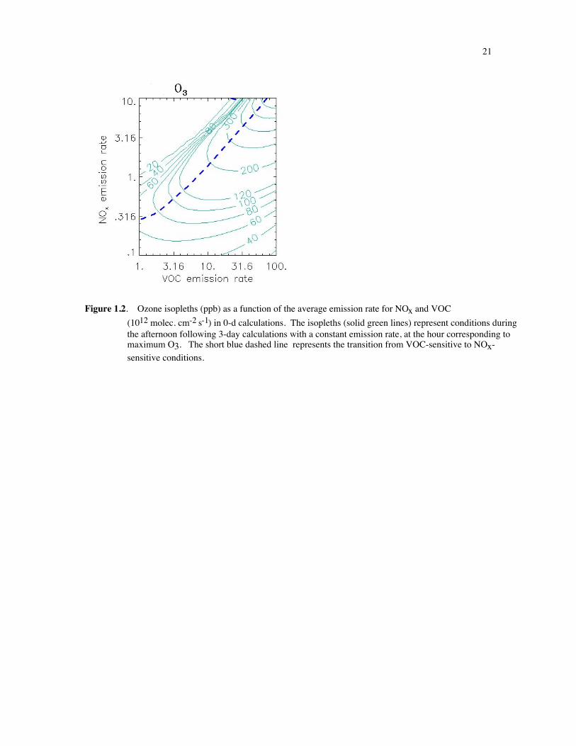
1.5 BACKGROUND INFORMATION ON O3-NOx-VOC SENSITIVITY

The relationship between O3, NOx-and VOC is illustrated in isopleth plots, e.g. Figure 1.2, which shows ozone

concentrations as a function of NOx and VOC emission rates. This particular plot is based on calculated

photochemistry for a 3-day period. Similar patterns are found for single-day calculations and for calculations that

relate instantaneous rates of ozone production to concentrations of NOx and VOC.

As shown in the figure, O3 shows a nonlinear dependence on NOx and VOC. O3 increases with increasing NOx

when NOx concentrations are low and when VOC/NOx ratios are high. As NOx increases, Ox eventually reaches a

maximum and then decreases in response to further increases in NOx. This maximum value (the ‘ridge line’) is

used to define two regions with different photochemistry and with different ozone precursor sensitivity. At high

VOC/NOx ratios (below the ‘ridge line’ in Figure 1.5.1) ozone increases with increasing NOx and is relatively

insensitive to increasing VOC. At low VOC/NOx ratios (above the ‘ridge line’) ozone increases with increasing

VOC and decreases with increasing NOx. The split between these two regimes is the source of much uncertainty in

control strategy predictions (see Section 1.4).

The split between NOx-sensitive and VOC-sensitive regimes is associated with the photochemistry of odd

hydrogen radicals (OH, HO2 and RO2 radicals) that control the rate of ozone production. The chemistry of ozone

production and radicals is described more fully in Section 3.1.12.

The split into NOx-sensitive and VOC-sensitive regimes also depends on the precise definition of the ‘ridge line’.

This can be defined as the location of maximum O3 (or the maximum rate of ozone formation) relative to variation

in NOx (NOx benefits versus disbenefits), or it can be defined as the location where identical percent reductions in

NOx and VOC would cause the same reduction in O3 (NOx-sensitive versus VOC-sensitive). This is discussed in

Section 3.1.10.

21

Figure 1.2. Ozone isopleths (ppb) as a function of the average emission rate for NOx and VOC(1012 molec. cm-2 s-1) in 0-d calculations. The isopleths (solid green lines) represent conditions duringthe afternoon following 3-day calculations with a constant emission rate, at the hour corresponding tomaximum O3. The short blue dashed line represents the transition from VOC-sensitive to NOx-sensitive conditions.

22

SECTION 2: SURVEY OF OBSERVATION-BASED METHODS

This section presents summary information about the approaches which have been proposed as OBM's and which

are capable of either replacing or supplementing standard AQM's for evaluating the relative impact of NOx and

VOC on ozone formation. This section also includes an evaluation of the strengths and weaknesses of each

approach and selection of approaches for in-depth investigation.

In addition, this section presents a brief summary of two additional topics that are linked to observation-based

methods: receptor modeling, which uses ambient measurements to identify emission sources of ambient species;

and methods for evaluating of long-term trends for ozone and other species. Evaluation of trends is especially

important as a basis for identifying whether past policies have been effective in reducing ambient concentrations and

for identifying the reasons for the success or failures of those policies.

2.1 CRITERIA FOR EVALUATION

Individual OBMs are discussed in terms of the following topics.

Theoretical basis: This refers to the rationale offered for why the particular OBM works successfully. This is

especially important for the OBMs that include simple rules for identifying whether ozone is primarily sensitive to

NOx or to VOC. The rules should be explainable in terms of ozone chemistry, rather than just a technique that

appears to work empirically.

Method of justification: OBMs typically must offer some type of test (in terms of model calculations or

experiments) to demonstrate that the information provided by the OBM is correct.

Range of applications: The range of apparently successful applications (consistent with the claims of the

method) will be presented here. In order to justify use, an OBM should be tested and applied successfully in many

different locations, preferably by several independent investigators. These tests should include applications that test

the validity of the method, as well as tests that just apply the method.

Contrary evidence: Applications that generate apparently contrary results are presented here.

Is it universal? In order to be used successfully, an OBM must be widely applicable in locations and situations

of interest for air quality management. Tests for the validity of an OBM should be sufficiently broad to demonstrate

that the concept works successfully in a range of conditions, rather than just in a small number of events or

23

locations. Limitation on the applicability of an OBM does not in itself prevent use of the OBM in air quality

management. However, the limitations of the OBM must be well understood, and it must be demonstrated that the

OBM is broadly applicable for the range of locations for which it is proposed.

Other sources of error: The most likely causes of error in individual applications are discussed here. This

includes situations in which the method might not return a useful answer as well as situations in which t he OBM

might lead to erroneous conclusions. The potential errors of OBMs are especially important in comparison to the

sources of error in standard AQMs.

Ease of use: In order to be used successfully in air quality applications, an OBM must be able to yield useful

answers for a reasonable amount of effort. Some levels of analysis may be useful as part of research efforts but

require a level of analysis that is beyond the scope of most investigations for air quality management. In addition,

the measurements required by an OBM must be available or potentially obtainable with a reasonable effort.

In this context, it may be necessary to caution against "rules of thumb" that are too simplistic.

Availability and accuracy of measurements: The required measurements must be either available from an

existing network or must involve equipment that is available and might be implemented with reasonable effort.

These measurements also must meet standards of accuracy.

Can the method be evaluated or modified in individual applications? Some OBMs consist of a single

procedure that would be applied for individual locations, with results that must be accepted on a "take-it-or-leave-it"

basis. It is a major advantage if an OBM also includes methods to evaluate the individual applications and identify

errors (e.g. erroneous measurements, conditions that invalidate the OBM for the specific applications, etc.) Existing

OBMs rarely include this type of evaluation. The possibility for developing such an evaluation is important to

consider in selecting OBMs for wider use.

Synthesis with Eulerian models: It is advantageous if an OBM can be applied in a way that complements the

use of standard AQMs.

Format for evaluation: The following section includes an overview of each method and discussion of the

performance of the method in relation to each of the above topics. Results for each topic will be presented based on

the available information on the OBM in published literature. Modifications or opinions offered by the author of

this report will be labeled as "comments". In addition, the label "controversial issue" is used to identify issues or

24

recommendations by the author that relate to central policy choices or to issues where disagreement is expected.

The presentation of each OBM is followed by a summary recommendation that describes the major advantages and

disadvantages of the approach and recommends possible further development.

2.2 OVERVIEW OF OBM APPROACHES AND ISSUES.

The following categories are useful for understanding the range of options among OBMs.

Primary species, secondary species, or radicals: Virtually all OBMs for ozone production rely on measurements

of chemically active species (e.g. as opposed to meteorological variables). Based on the choice of measurements,

three general approaches can be identified. Several methods rely on measurements of directly emitted ozone

precursors, usually speciated VOC and NOx. A second grouping involves measurements of long-lived secondary

species (e.g. reactive nitrogen) that are produced concurrently with the production of ozone. A third grouping is

based on direct or indirect measurement of short-lived radical species (e.g. HO2).

These three approaches also imply different strategies of analysis. Analysis based on primary species typically

provides information about the ozone production that will occur in the future as the measured precursor species

move downwind. Analysis based on secondary species provides information about the ozone production that has

already occurred upwind at the time of measurement. These two approaches are largely complementary in that they

can provide information on the same issue (impact of VOC versus NOx) using different evidence. They also require

different measurement strategies. Primary species need to be measured near major emission sources and in regions

with high ozone production; whereas secondary species need to be measured downwind in locations with the

highest ambient ozone. Analysis based on radical species only provides information about instantaneous ozone

production.

Models versus smog chambers: A major distinction between OBMs concerns the method used to obtain the

interpretation of measurements used in the OBM and to prove its validity. Some methods (e.g. Sillman, 1995) use

3-d Eulerian photochemical models (similar to standard AQMs) to identify measurements and interpretations that

can be used as an OBM. Others (e.g. Blanchard et al., 1999) use smog chamber experiments to interpret

measurements.

Instantaneous production versus ozone concentrations: Elevated ozone usually is the result of combined

photochemistry and transport over a time period of several hours or more (often including time periods greater than

25

one day). The relation between ozone concentrations and its precursors is complicated by the mix of fresh and aged

emissions and changing photochemistry as an air mass travels downwind from emission source regions. Some

OBMs seek to identify the impact of upwind VOC and NOx precursor emissions on the total ozone concentration,

while others seek to identify the impact of local emissions on the instantaneous rate of ozone production.

It is important to recognize that the instantaneous dependence of ozone photochemistry on NOx and VOC is

often very different from the sensitivity of ozone concentrations to upwind NOx and VOC. It is generally easier

and more reliable to derive information about the factors that control the instantaneous rate of ozone production than

it is to derive information about the total impact on ozone as emissions from a source move downwind. However,

information about instantaneous chemistry is more difficult to interpret in the context of policy.

Definition of NOx-VOC sensitivity: The OBMs included in this survey are all intended to aid in evaluating the

relative impact of NOx and VOC on ozone formation. Results of these OBMs often depend on how terms such as

"NOx-sensitive" and "VOC-sensitive" are defined. A summary of various alternative definitions is presented here.

NOx-sensitive versus VOC-sensitive: The term "NOx-sensitive" will be used to describe a situation if a given

reduction in NOx emissions is expected to cause a significant decrease in O3, and if O3 with reduced NOx

emissions is also expected to be significantly lower than O3 with an equivalent reduction (as a percent of total

emissions) of anthropogenic VOC.

Similarly, the term "VOC-sensitive" will be used if a given reduction in anthropogenic VOC emissions is

expected to cause a significant decrease in O3 and is expected to result in significantly lower O3 than an equivalent

reduction (in proportion to total emissions) of anthropogenic NOx.

In this definition, "significant" is an ambiguous term that depends on the individual situation. Here, it is assumed

that "significant" refers to the physical context of the situation and not the policy context. Typically, OBMs can

provide information on how the expected decrease in O3 resulting from reduced NOx compares to the expected

decrease in O3 from an equivalent reduction in VOC. They do not provide information on whether these reductions

are significant in terms of policy.

The above definition can be used in reference to ozone concentrations or to instantaneous production rates.

26

NOx benefits versus disbenefits: An alternative way to define control predictions is to define situations based on

whether reductions in NOx emissions would lead to a decrease in O3 (NOx benefits) or an increase in O3 (NOx

disbenefits). This distinction is often important in terms of policy.

This definition is different from the definition of NOx-sensitive and VOC-sensitive given above in that many

VOC-sensitive situations still have predicted small benefits rather than disbenefits from NOx controls. Tonnesen

and Dennis (2000b) discussed the difference between the two definitions in detail.

VOC benefits versus zero impact: Lu and Chang (1998) and Kirchner et al. (2000) both made an additional

distinction between locations in which reduced anthropogenic VOC has a negligibly small impact on ozone, as

opposed to locations in which reduced anthropogenic VOC causes some reduction in ozone. In their definition,

situations in which reduced VOC would cause a nonzero ozone reduction would be regarded as sensitive to both

NOx and VOC, even if reduced NOx had a much larger impact than the equivalent percent reduction in VOC.

NOx titration without VOC benefits: In situations in the vicinity of very large NOx emissions sources, it

frequently is predicted that ozone would increase in response to reduced NOx emissions, but would be virtually

unaffected by reduced VOC. This situation occurs only when the rate of photochemical formation of ozone (via

NO-to-NO2 conversions) is negligibly small. Ozone would decrease in response to NO emissions because NO

removes Ox through the reaction

NO + O3 Æ NO2 + O2 (1)

The process also occurs at night, when there is no significant photochemical production of O3.

In some analyses, a distinction is made between situations dominated by NOx titration (in which VOC emissions

have little effect) and situations with standard VOC-sensitive or NOx saturated chemistry, in which ozone increases

with increasing VOC.

Extent of NOx and VOC reductions: The relative impact of reduced NOx and VOC is often very different for

large reductions (as a percent of total emissions) as opposed to small reductions. In general, NOx controls appear

more advantageous relative to VOC when very large percent reductions are considered, while VOC controls appear

more advantageous relative to NOx if relatively small changes are made. It is quite common for a location to be

27

"VOC-sensitive" with respect to emission reductions of 25% and "NOx-sensitive" with respect to emission

reductions of 75% (Roselle and Schere, 1995).

Definitions used in this study: Unless otherwise stated, this study will use the terms “NOx-sensitive” to refer to

situations in which significantly greater reduction in O3 is expected from reduced NOx relative to an equivalent

percent reduction in VOC, and “VOC-sensitive” for the opposite. Some subsections will refer to studies that define

sensitivity in terms of NOx benefits versus disbenefits. These will be referred to as “NOx-sensitive” versus “NOx-

saturated”. Some sections will also use NOx titration as an additional classification. Unless otherwise specified,

these terms will all be used with reference to emission reductions in anthropogenic NOx and VOC of 25%-50%.

2.3 EVALUATION OF INDIVIDUAL OBMs

2.3.1. Secondary species as NOx-VOC indicators

Overview: NOx-VOC indicators refers to a series of species and species ratios, usually involving reactive

nitrogen, that are believed to be linked to O3-NOx-VOC sensitivity. The method is based on the concept that when

ozone concentrations are sensitive primarily to NOx rather than VOC, measured values of these indicator ratios are

high. When ozone concentrations are sensitive primarily to VOC rather than NOx, measured values of the indicator

ratios are low.

The indicator ratios are associated with NOx-VOC sensitivity only at the exact time and place of measurement.

Measured values at one location and during a single event do not provide any information about NOx-VOC

sensitivity at a different location or at the same location during a different event. Consequently, the method can be

used only when there is an extensive network of measurements that includes the region where peak O3 occurs.

The original work on this concept (Sillman, 1995) identified two major classes of ratios that were likely to serve

as NOx-VOC indicators: (i) O3/NOy (where NOy represents total reactive nitrogen) and the closely related ratios

Oy/(NOy-NOx) and O3/HNO3; and (ii) H2O2/HNO3 and a series of similar ratios involving peroxides and reactive

nitrogen. Subsequent researchers identified slightly different variations. Other proposed indicator ratios (NOy,

HCHO/NOy, and O3/NOx) were subsequently found to have major flaws.

The concept of indicator ratios was originally developed by Milford et al. (1994), Sillman (1995) and Sillman et

al. (1995, 1997, 1998, 2001a, 2001b) and subsequently analyzed by Tonnesen and Dennis (1998), Lu and Chang

28

(1998), Chock et al. (1999), Vogel et al., 1999, and Martilli et al., 2001. Tonnesen and Dennis (1998) extended the

concept and investigated various alternative indicator ratios (see additional results in Section 2.3.3).

Theoretical basis: The main indicator ratios (O3/NOy and H2O2/HNO3) were both justified in terms of radical

chemistry. Instantaneous ozone chemistry is sensitive to NOx when the rate of conversion of radicals to peroxides

exceeds the rate of conversion to HNO3, or (alternatively) when the rate of production of radicals exceeds the rate of

removal of NOx. Based on this radical chemistry, NOx-sensitive conditions should be associated with high values

of O3/NOy and H2O2/HNO3.

Comment: The ratio O3/NOy can also be interpreted as ratio of ozone production to NOx removal, or ozone

production efficiency per NOx (Trainer et al., 1993). This ozone production efficiency is higher in NOx-sensitive

conditions based on either the radical chemistry above or the higher VOC/NOx ratios associated with NOx-sensitive

conditions. The ratio O3/NOy also is affected by photochemical age (see discussion of smog production algorithms

in Section 2.3.2 below).

Method of justification: The NOx-VOC indicators are identified from 3-d Eulerian simulations, including

standard AQMs. Initial model scenarios are repeated with 25%-50% reductions in domain-wide emissions of

anthropogenic VOC and of NOx in order to obtain the predicted response to VOC and NOx controls. These control

predictions are correlated with the value of the proposed indicator ratios in the model base case. The test

simulations include perturbed scenarios with changed base case emissions and meteorology in order to insure that

the apparent relationship between NOx-VOC sensitivity and indicator ratios is not dependent on model assumptions.

Range of applications: Tests for the validity of the indicator method require the use of 3-d Eulerian models,

although measurement-based applications can provide supporting evidence by showing whether measured species

are consistent with the range of model predictions. Applications with model-based tests of validity include the

following locations: the northeast corridor and Lake Michigan airsheds (Sillman, 1995); Atlanta* (Sillman et al.,

1995); New York and Los Angeles* (Sillman et al., 1997); Nashville* (Sillman et al., 1998); the eastern U.S.

(Tonnesen et al., 2000a); Switzerland (Staffelbach et al., 1997, Dommen et al., 1999) Milan, Italy* (Martilli et al.,

2001, Hammer et al., 2001); and Paris, France* (Sillman et al., 2001). Many of these applications (identified by

asterisks) included measurements and model-measurement comparisons for the relevant species. Tests that

generated contrary evidence are listed below. The tests included several different photochemical mechanisms:

29

Sillman's mechanism based on Lurmann et al. (1986); CB4 (Gery et al., 1989), and mechanisms based on EMEP in

Europe.

Contrary evidence: Model-based investigations of the San Joaquin valley (Lu and Chang, 1998) and in Los

Angeles (Chock et al., 1999) both generated results for NOx-VOC indicators that differed substantially from the

results reported by Sillman, above. Blanchard and Stoeckenius (2001) also reported contradictory results in a

review that included the above model applications. Both sets of contrary results used CB-4 chemistry. West et al.

(2000) found contrary results from a model-based investigation in Mexico City. Blanchard et al. (2001) reported

that the method was successful qualitatively, but that indicator values varied with individual applications. Results

from Paris, France (Sillman et al., 2001) also identify situations where measurements may not be of sufficient

accuracy.

Is it universal? It is uncertain whether the original NOx-VOC indicators are broadly applicable or if their use

varies from location to location. NOx-VOC indicators were originally presented as a concept that would be

universally valid. Consistent results were obtained for many different locations and model types. However, the

contrary results for San Joaquin and Los Angeles suggest that the NOx-VOC indicators may show significant

variation among different locations. It is likely that a modified version of the indicator formula would be valid even

in these cases, but it is unclear whether a modified formula would have universal validity or if it would need to be

adjusted for each location.

The NOx-VOC indicators can only be used during a prescribed range of conditions: afternoon (between 1 pm

and sunset) during relatively sunny days and without rain.

Other sources of error: NOx-VOC indicators would return misleading results in situations where HNO3 were

removed from the ambient atmosphere (by deposition or by conversion to aerosol nitrate) much more rapidly than

currently represented in AQMs. Similarly misleading results would occur if measured NOy did not include HNO3.

Measured (NOy-HNO3) apparently cannot be used evaluating NOx-VOC sensitivity.

Ease of use: The NOx-VOC indicators require an extensive network of measurements and care to insure

measurement accuracy. If measurements are available, the method itself consists of a simple "rule of thumb" that

identifies NOx-sensitive and VOC-sensitive regions. A thorough application of the method would include testing

with an AQM and evaluation of measured species correlation patterns in comparison with model results. This

30

evaluation would require the development of detailed protocols, but would probably be no more difficult then

existing evaluation of AQM results versus measured O3. Some additional interpretation is also needed if the NOx-

VOC indicators are used to evaluate 8-hour average O3.

Availability and accuracy of measurements: Among the proposed indicator ratios, only O3/NOy (and possibly

O3/(NOy-NOx) and O3/HNO3) can be considered for widespread regulatory use. The NOx-VOC indicators

involving peroxides appear to be more accurate, but peroxides require a research-grade measurement. O3, NOx and

NOy can be measured using commercially available instruments.

The EPA PAMs network currently measures NOy at a small number of sites in the northeast. These are all rural

sites and are less likely to have unusually high O3. Widespread application of the indicator method would be

possible only if this network were expanded. In addition, there are issues of measurement accuracy. The indicator

method requires measured NOy with uncertainties less than 20% (preferably less than 10%). NOy measurements are

subject to error if HNO3 is lost in the measurement inlet tube. Such an error would render the measurement invalid

for use as a NOx-VOC indicator.

Can the method be evaluated or modified in individual applications? Because NOx-VOC indicators are

generated by AQMs, routine application of AQMs in the regulatory process can also be used to evaluate and modify

the NOx-VOC indicators for specific locations and events. It is more difficult to evaluate measurements associated

with applications of the indicator method.

Synthesis with Eulerian models: NOx-VOC indicators can be used to evaluate the accuracy of individual AQM

applications, in the same way that measured O3 has been used in the past. Because NOx-VOC indicators are

closely associated with Eulerian AQMs, there are various ways in which AQMs and indicator measurements can be

used in combination. In cases where measured indicator ratios are consistent with results of a regulatory AQM, they

provide a stronger basis for confidence in the AQM than would be provided by measured O3 alone. However, it is

unclear how to respond in a case where major differences appeared between the AQM and measured indicator

ratios.

Overall evaluation: Indicator ratios have a number of advantages for regulatory use as an OBM. They have

been applied and tested very widely. There has been more contrary evidence for the NOx-VOC indicators than for

other methods, but this may be due to the fact that indicators have been tested more extensively than other methods.

31

The simplest indicator ratio (O3/NOy) can be used with commercially available instrumentation, and the method can

be evaluated and updated separately even in regulatory applications. The most promising use of indicator ratios

would be to evaluate the accuracy of individual applications of Eulerian AQMs. Use of measured indicator ratios to

evaluate AQMs would probably remain valid even if it were found that the indicator ratios failed as a stand-alone

method to evaluate ozone control strategies.

Case studies with NOx-VOC indicators have given mixed results. In some instances the NOx-VOC indicators

seemed to provide clear evidence for NOx-sensitive or VOC-sensitive conditions, but in other cases the indicator

values were uncertain. Interpretation of NOx-VOC indicators must account for the sources of error discussed

above.

If NOx-VOC indicators were used in regulatory applications, protocol would need to be developed for situations

in which results from indicators and results from AQMs disagreed. In some cases AQMs may predict NOx-sensitive

conditions while measured indicator ratios suggest VOC-sensitive conditions, or vice versus. It would then be

necessary either to correct the regulatory AQM or to reject the evidence from indicators.

There are important opportunities for synthesis between NOx-VOC indicators and smog production algorithms,

described in Section 2.3.2.

2.3.2. Smog production (extent-of-reaction) algorithms

Overview: Smog production algorithms are methods of evaluating O3-NOx-VOC sensitivity based on ambient

measurement of a few species, primarily reactive nitrogen. The distinctive feature of smog production algorithms

(as opposed to the NOx-VOC indicators discussed in Section 2.3.1) is that they were initially derived based on smog

chamber experiments rather than 3-d Eulerian models. The smog production algorithms are also based on a specific

rationale: the belief that VOC-sensitive conditions are associated with relatively fresh emissions and that NOx-

sensitive conditions are associated with aged air in which ozone producing reactions have been run to completion.

The smog production algorithms all use measurements to infer the maximum smog production for the given amount

of ozone precursors (SPmax) in comparison with actual smog production (SP). The ratio (SP/SPmax) is referred to

as the extent of reaction, and high values are associated with NOx-sensitive conditions. The extent of reaction is

obtained from formulas based on measured O3, NO, and either NOx and NOy. The main formulas use variants of

the ratios O3/NOy, O3/NOx and NOx/NOy, each measured in locations with high O3.

32

As with the NOx-VOC indicators, the smog production algorithms provide information on O3-NOx-VOC

sensitivity only at the exact time and place of measurement.

The smog production concept was originated by Graham Johnson (1984, 1989) and subsequently extended and

modified by Hess et al. (1992), Olszyna et al. (1994), T. Chang et al. (1997, 1998) and Blanchard et al. (1999, 2000,

2001). The extensions have included modifications based on additional smog chamber experiments and 0-d model

calculations, tests with 3-d Eulerian models, and limited confirmation of the theory based on ambient data. Smog

production algorithms have been used to diagnose O3-NOx-VOC sensitivity extensively in the U.S. (in the New

York-Connecticut-Massachusetts and Baltimore-Washington corridors, Atlanta, Houston and other cities in Texas,

Chicago, Los Angeles and the San Joaquin Valley) and in Australia (Melbourne).

Theoretical basis: As described above, the smog production algorithms are based on the concept that VOC-

sensitive conditions occur when precursor emissions are relatively fresh and have not reacted to completion, and that

NOx-sensitive conditions occur when precursors have reacted to completion. This "extent of reaction" refers to the

extent of reaction of NOx. NOx-sensitive conditions occur when most of the emitted NOx has already been

processed and converted to product species.

Comment : The notion that VOC-sensitive conditions are associated with relatively unprocessed emissions and

NOx-sensitive conditions are associated with aged air is often true, but it is not always true. There is extensive

evidence from smog chambers (e.g. Blanchard et al., 1999), 0-d and 3-d model calculations (Milford et al., 1994,

Blanchard et al., 1999) and some ambient measurements (Olszyna et al., 1994) to support this concept. However

there is also contrary evidence from 3-d models (Sillman and He, 2001). In addition, the theoretical basis assumes

that maximum smog production (SPmax) is a simple function of the initial NOx concentration. Recent evidence

from power plants (Ryerson et al., 1998, 2001) suggests that plumes with different amounts of biogenic VOC

produce different amounts of ozone, even after all the NOx has reacted away.

The finding that VOC-sensitive chemistry has low ozone production per NOx and that NOx-sensitive chemistry

has high ozone production per NOx may provide a stronger justification for the smog chamber algorithms. The

smog production formulas based on O3/NOy have values that reflect the rate of ozone production per NOx as well as

extent of reaction.

33

Method of justification: The smog production algorithms were derived from experiments in outdoor smog

chambers at CSIRO (Australia), University of North Carolina and University of California, Riverside and from 0-d

or box model calculations (Blanchard et al., 1999). Both the smog chamber and 0-d calculations represented an

initial high concentration of ozone precursors followed by photochemical reaction without additional emissions (or,

occasionally, with a second single burst of emissions). Sensitivity to NOx and VOC was inferred by comparing

experiments or calculations with changes in initial NOx and VOC concentrations. Results of 3-d models were also

used to test the accuracy of the smog production algorithms.

Range of applications: Smog production algorithms have been used very widely to diagnose O3-NOx-VOC

sensitivity in urban areas (e.g. T. Chang and Suzio, 1995, 1996; Blanchard, 2001), but most of these cases have

simply been applications of the smog production formula rather than evaluations of its validity. The validity of the

smog production algorithms is based on the range of smog chamber experiments, and includes experiments by three

groups (CSIRO, University of North Carolina and University of California, Riverside). The validity of smog

production algorithms has also been established by 0-d model calculations with two photochemical mechanisms:

CB-4 and Lurmann et al., 1987. Evaluation of the smog production algorithms based on 3-d models has been

performed for episodes in southern California, the San Joaquin Valley, Texas (near Houston), Lake Michigan and

the northeast corridor (T. Chang et al., 1997; Blanchard et al., 2001). The 3-d model tests were done with the

Urban Airshed Model (UAM-IV and UAM-V) and San Joaquin Air Quality Model (SAQM), both with CB-4

chemistry. In addition, ambient measurements in rural Tennessee were used to identify the pattern of ozone

production versus extent of reaction (Olszyna et al., 1994). This measurement-based investigation found a pattern

similar to that observed in smog chamber experiments.

Contrary evidence: Sillman (1999) and Sillman and He (2001) found that the smog production formulas based

on the ratio NOx/NOy do not correlate well with NOx-VOC sensitivity in 3-d models (for the northeast corridor and

Lake Michigan regions). The poor correlation was found in regional-scale models that included transport over 500

km or more, rather than a single city. The accuracy of smog production formulas based on NOx/NOy has never

been demonstrated in a 3-d model.

34

Blanchard et al. (2001) and Sillman and He (2001) also reported somewhat ambiguous results from 3-d

simulations for algorithms based on the ratio O3/NOy. Blanchard (2000) identified uncertainties based on

measurements of NOx from commercial instruments.

Is it universal? The smog chamber experiments suggest that the smog production algorithms are at least

qualitatively valid for a wide range of conditions. Results from 3-d models reported by Blanchard et al. (2001)

suggest that the exact transition from NOx-sensitive to VOC-sensitive conditions may vary in different locations.

Blanchard et al. (2001) found that there is a large range of values with uncertain NOx-VOC sensitivity, and only

extreme values of the smog production parameter can be definitely correlated with NOx-sensitive or VOC-sensitive

conditions everywhere. The smog production formula based on O3/NOy may be less subject to variation than the

indicator ratios used by Sillman (1995) because they are not affected by background conditions.

As was the case with NOx-VOC indicators (Section 2.3.1), the smog production algorithms cannot be used if

most of the NOy associated with ozone production has been removed by deposition. This prevents the use of smog

production algorithms at night or in events with precipitation.

Other sources of error: Smog production algorithms based on measured NOy are subject to error based on the

uncertain rate of removal of NOy from the ambient atmosphere. There are also possible errors in NOy

measurements. Smog algorithms that use NOx instead of NOy are less subject to uncertainty due to deposition.

However the smog production algorithm based on NOx has not been tested in 3-d models.

Ease of use: Smog production algorithms require measured O3, NO and either NOx or NOy. As with the NOx-

VOC indicators, these measurements must be extensive enough to characterize the entire area of peak O3. If

measurements of sufficient accuracy are available, application of the smog production algorithms is straightforward.

The smog production formula generates a measurement-based index that identifies NOx-sensitive and VOC-

sensitive locations.

Availability and accuracy of measurements: O3 and NOx measurements are both widely available through the

PAMs network, although there is some question about the accuracy of NOx measured by commercial instruments

(Winer et al., 1974, Logan, 1989). Blanchard (2001) included sensitivity to measurement error in applications of

smog production algorithms. NOy is less readily available, but instruments to measure NOy are commercially

available. The same concerns about accuracy associated with NOx-VOC indicators (above) apply here.

35

Can the method be evaluated or modified in individual applications? The smog production algorithms

represent a universal formula based on smog chambers and cannot be modified for individual applications. The

method also does not include a way to evaluate the accuracy of measurements used in individual applications,

although Blanchard (2001) included analysis of sensitivity to measurement uncertainties in their applications. The

accuracy of smog production algorithms can be evaluated in individual applications if an AQM is used.

Synthesis with Eulerian models: Smog production algorithms were developed independently from Eulerian

AQMs, and there are no immediately obvious ways to develop a synthesis. However, smog production algorithms

can probably be extended for use as a tool to evaluate the accuracy of AQM scenarios. Combined use of AQMs

and smog algorithms can be done in the same way as combined use of AQMs and NOx-VOC indicators. It is

unclear how to respond when AQMs and smog production algorithms lead to opposite conclusions in terms of

control strategies.

Overall evaluation: Smog production algorithms are currently the most widely used OBM, especially in

regulatory applications. Research on the method has included many investigators and involved limited evaluation

with 3-d model calculations and some analysis of ambient data in addition to the extensive smog chamber

experiments. It can be incorporated easily into existing regulatory evaluations and can be used with measurements

currently available from the PAMs network.

Its major drawback is vagueness about uncertainties when the method is applied to ambient conditions. In most

applications the method has been used as a plug-in formula, used to provide answers with relatively little

investigation of its accuracy. The rate of removal of NOy, a critical parameter and source of uncertainty, is not

included in the algorithms and is instead left for users to estimate. There is also no clear guidance for identifying

background O3, which is an important parameter in most of the smog algorithms. The method could be improved if

it were combined with a broader analysis of ambient measurements and with comparisons between measurements

and model results.

Of the three types of smog production algorithms, the algorithm based on O3 and NOy appears to be the most

accurate. The method based on NOx and NOy was found to give poor results when tested in 3-d air quality models

(Sillman, 2000; Sillman and He., 2001). The method based on O3 and NOx also appears to give ambiguous results

when tested in air quality models.

36

The smog production algorithms closely resemble some of the NOx-VOC indicator formulations. Some of the

problems associated with smog production algorithms might be addressed based on results from investigations of the

indicator formulas, while some of the problems associated with indicators might be addressed by using results from

the smog production algorithms. A combination of the two methods might be useful.

Controversial issue – models versus smog chamber results: The major issue for smog production algorithms

concerns the level of confidence in smog chamber experiments as a basis for developing an OBM. By contrast,

NOx-VOC indicators were developed based on 3-d Eulerian models. Reliance on 3-d models has several

advantages. Indicators derived from models can be evaluated and modified for individual situations based on results

from AQMs. Indicators can also be used to provide a broader evaluation of the accuracy of AQMs, and these

evaluations can also expose flaws in the indicator formula or in the accuracy of individual measurements. The

models used to derive indicators include a more detailed representation of the geographic pattern of emissions and

include multiday transport. Smog chambers, by contrast, represent a single emission source followed by chemical

evolution without added emissions. Such conditions rarely occur in the ambient atmosphere.

Here, it will be assumed that smog production algorithms are valid only when they can be shown to perform

successfully in 3-d models.

2.3.3. Constrained steady state (CSS): Instantaneous chemistry based on measured NOx and VOC

Overview: The constrained steady state method (CSS) is presented here as a combination of two similar

methods that have been developed independently: one by Kleinman et al. (1997, 2000, 2001) and the other by

Tonnesen and Dennis (2000b). Kirchner et al. (2001) also proposed a similar method. Although no intercomparison

has been made, the methods appear to use the same species and the same strategy. The observation-based model

developed by Cardelino and Chameides (1995, 2001) is also closely related but is discussed separately (see section

2.3.4).

Both methods seek to evaluate the instantaneous rate of production of O3 and how it depends on NOx and VOC.

Both methods are based on the use of measured primary species (NOx and VOC). Both methods derive a relation

for NOx-VOC sensitivity in terms of radical budgets. Both also derive indicators for instantaneous NOx-VOC

sensitivity in terms of a reactivity-weighted sum of VOC and NOx. Tonnesen and Dennis derive a formula with the

form kiVOCiiÂ ( kiVOCiiÂ + kn NO2 ) , where VOCi and NO2 represent measured quantities. An

37

equivalent formula based on a simple ratio of summed reactivity-weighted VOC to NOx could also be developed. A

formula based on the ratio of reactivity-weighted VOC to NOx was also proposed informally by Chameides et al.

(1992). Kleinman et al. derive a more complex formula involving VOC, NOx and the total radical source

(calculated or inferred from measured VOC). Tonnesen et al. also derive an indicator based on summed organic

peroxy radicals (RO2), but this is not immediately useful for regulatory applications due to the scarcity of

measurements.

Kleinman et al. also use a series of 0-d calculations ('constrained steady state') driven by measurements, which

can be used to derive the NOx-VOC dependence of the instantaneous rate of ozone production. This type of steady-

state calculation is frequently used to evaluate ozone production in the remote troposphere (e.g. Ridley et al., 1992,

see also Jaegle et al, 1998, 2001). Kleinman et al. represent the only attempt to do a similar analysis in polluted

locations.

Theoretical basis: Kleinman et al. and Tonnesen and Dennis both derive their analyses based on radical

chemistry. NOx-sensitive chemistry is associated with conditions in which formation of peroxides represents the

dominant sink for the family of radicals (including OH, HO2 and RO2), while VOC-sensitive chemistry is

associated with conditions in which formation of nitric acid represents the dominant sink for radicals. The link

between instantaneous NOx-VOC sensitivity and reactivity-weighted VOC and NOx is derived from radical

chemistry.

Comment : This is similar to the rationale proposed for NOx-VOC indicators. Since it involves instantaneous

chemistry rather than the more complex chemistry and transport that affect ozone concentrations, it is more likely to

be universally true.

Method of justification: Kleinman et al. justify their methods through a series of steady-state calculations,

which represent instantaneous chemistry. Tonnesen and Dennis used trajectory model calculations (OZIPR, familiar

as part of the EKMA modeling approach) and results of a 3-d AQM. Because this method focuses on instantaneous

photochemical production, the 3-d model results were used largely to provide a series of photochemical calculations

for a range of conditions. Kleinman et al. and Tonnesen and Dennis both used RADM2 chemistry (Stockwell et al.,

1990). Kleinman et al. incorporated the mechanism of Paulson and Seinfeld (1992) for isoprene.

38

Range of applications: Kleinman et al. applied their method (including both 0-d model calculations and

measurements) to cases in Phoenix, AZ and New York City. Tonnesen and Dennis presented model results only,

using an EKMA model for Atlanta and a RADM simulation for the northeastern U.S.

Contrary evidence: None.

Is it universal? The instantaneous chemistry formulas have been developed based on a small number of cases

and only one photochemical mechanism (RADM2). However, there is reason to believe that a variation of the

method with universal validity can be developed. Constrained steady state calculations have been used very widely

to evaluate instantaneous photochemistry in the remote troposphere. These calculations are equivalent to 3-d

AQMs in terms of being universally applicable, and are less sensitive to model parameters or assumptions than the

AQMs. The abbreviated formulas as functions of measured VOC and NOx were presented by Kleinman et al. and

Tonnesen and Dennis as universal derivations from radical chemistry. Due to the complex nature of VOC

chemistry, much more extensive testing and analysis is needed to establish whether the formulas have universal

validity.

Other sources of error: All variants of the instantaneous chemistry formula rely on measured VOC and NOx,

and are subject to errors common to all methods that depend on these measurements:

• Surface ozone concentrations result from photochemical production throughout the daytime convective

mixed layer, which typically extends to a height of 1000-2000 meters. VOC and NOx concentrations vary

significantly with height, and surface measurements (which are most commonly available) do not reflect this

variation. This is especially true for biogenic VOC.

• Measured VOC and NOx at the surface are often affected by emission sources in the immediate vicinity of

the monitor, and may therefore not be representative of average conditions in the area.

• Concern has been expressed that measured VOC from the EPA PAMs network may underestimate the

amount of alkenes and other highly reactive VOC (Parrish et al., 1998, 2000). If these species are

underrepresented, the method will return biased results.

• Concern has been expressed that measured NOx using commercially available instruments represents the

sum of NOx and various NOx reaction products (Winer et al., 1974, Logan, 1989, Blanchard, 2001). This

39

would compromise the use of the method. In addition, Cardelino and Chameides (2000) found that

measured NO may not be of sufficient accuracy to distinguish NOx-sensitive from VOC-sensitive chemistry.

Ease of use: Because these formulas represent instantaneous photochemistry only, they require considerable

interpretation in order to be used in regulatory applications. The major regulatory concern is the relation between

ozone concentrations and precursor emissions. Currently there is no clear method available for using the formulas

for instantaneous chemistry to address regulatory concerns.

The formula developed by Tonnesen and Dennis is represents a one-step calculation and can be made easily from

measured VOC and NOx. The formula developed by Kleinman et al. requires more effort. The steady-state model

used by Kleinman et al. has the same level of complexity as traditional 0-d or box models. This is considerably

simpler than the current generation of 3-d AQMs. Such a model could be easily developed for regulatory use

(especially if linked to the format of available measurements), but an easy-to-use version is not currently available.

Availability and accuracy of measurements: The methods that are most likely to be of practical use would

require complete sets of measured VOC and NOx at locations spread throughout the area of interest. Because the

calculations are only valid for the exact time and place of measurements, the network would need to be extensive.

Kleinman et al. present an alternative formula that does not need complete measurement of VOC. However, the

alternative would require measured formaldehyde (HCHO) and would probably require other aldehydes and alkenes

(as radicals sources) as well. This is likely to be just as difficult as complete primary VOC.

Primary VOC and NOx measurements are generally available through the EPA PAMs network. Concern about

the accuracy of these measurements is discussed above (see sources of error).

Can the method be evaluated or modified in individual applications? The constrained steady state

calculation is a universal calculation and would not be modified in individual applications. It might be possible to

modify the instantaneous formulas for individual applications, using results from individual AQMs (in effect

duplicating the work of Tonnesen and Dennis), though this would be laborious.

Synthesis with Eulerian models: The VOC-NOx formula developed by Tonnesen and Dennis could be used as

a basis for evaluating the accuracy of AQM applications. Given that this formula is related to NOx-VOC chemistry,

it could be expanded into a general evaluation of the accuracy of AQM representation. This would remain true even

if it were found that the formula was imprecise as a NOx-VOC indicator. The VOC-NOx formula is also useful

40

because it relates to emissions in an AQM, and might be used to as a basis for generating a modified AQM scenario.

The steady state calculation developed by Kleinman et al. could be used similarly, although it does not have a direct

connection to emissions in AQMs.

Overall evaluation: Of the various proposed OBMs proposed for evaluating NOx-VOC sensitivity, the

instantaneous formulas are the most strongly grounded in scientific principles and have the strongest claim to

universal validity. The CSS calculation in particular is widely used in investigations of tropospheric chemistry and

is likely limited only through the extent and accuracy of the available measurements. The concept of NOx-VOC

sensitivity developed by Kleinman et al. is also being used in research projects that evaluate the accuracy of current

representations of ozone photochemistry (Thornton et al. 2002) However, the instantaneous formulas do not

represent the complete process of photochemistry and transport that causes elevated ozone. In many ways the

higher degree of scientific validity occurs because they omit the processes that are most difficult to analyze.

The instantaneous formula based on VOC and NOx is especially interesting because measured VOC and NOx

have often have been used as a diagnostic tool for ozone. Throughout the 1980's it was thought that O3-NOx-VOC

sensitivity could be evaluated based on the ratio of VOC to NOx measured in an urban center during the early

morning. This morning VOC/NOx ratio was subject to many errors as a basis for determining NOx-VOC

sensitivity: it did not account for reactivity of individual VOC; it did not account for biogenics; and it did not

account for the transport process. However, a formula based on reactivity-weighted VOC and NOx may be

generally applicable as a way to evaluate instantaneous photochemistry. With this understanding, measured VOC

and NOx might be used more appropriately in the regulatory process.

The formula for instantaneous O3-NOx-VOC sensitivity based on measured VOC needs to be tested with other

photochemical mechanisms and for a wider range of conditions. It should also be compared with the analysis of

ozone formation potential (e.g. Carter et al., 1994, 1995).

The question of the vertical distribution of individual VOCs and the possibility of influence from sources in the

immediate vicinity of measurement sites are likely to be the greatest challenge for this method.

The observation-based model of Cardelino and Chameides (Section 2.3.4 below) is closely related to this

method.

2.3.4. Observation-based model using NOx and VOC (Cardelino-Chameides)

41

Overview: The observation-based model developed by Cardelino and Chameides (1995, 2000) was developed

directly in response to the perceived deficiencies of AQMs and the need for observation-based methods. It was

originally described as a model calculation that would duplicate many features of AQMs ('emission-based models')

but would use ambient measurements in place of emission inventories to determine concentrations of primary

pollutants.

The observation-based model consists of a series of 0-d or box model calculations constrained by measured O3,

NOx and VOC. These calculations are similar to the constrained steady state (CSS) calculations developed by

Kleinman et al. (above), but they also include the impact of vertical diffusion. Overall impact of emitted NOx and

VOC on O3 is assessed by repeating the calculation with reduced NOx and VOC, following a methodology similar

to the studies of relative incremental reactivity by Carter et al. (1994, 1995). The overall impact of NOx and VOC

within a metropolitan area is assessed by a sum of relative incremental reactivities (weighted by ozone production

rates) for each hour during the period of ozone production and for each measurement site.

The observation-based model grew out of work by Chameides et al. (1992), which is discussed in connection

with NOx-VOC isopleths, below.

Theoretical basis: The method consists of model calculations rather than a formula or rule of thumb. No

specific rationale is needed in this case. The major theoretical issue concerns whether the factors controlling ozone

concentrations (including transport over a wide range of conditions) can be adequately represented by a series of 0-d

calculations, which represent conditions at discrete times and locations.

Method of justification: The OBM calculations are viewed as having universal validity by themselves,

equivalent to 3-d Eulerian AQMs. In addition, the calculations have been compared with results from AQMs for a

series of scenarios in Atlanta.

Range of applications: The only complete analysis based on a network of measurements throughout an urban

area was done for Atlanta. This analysis also included extensive comparisons with an Eulerian AQM. Other

applications were developed for individual measurement sites in Washington D.C., New York and Texas. Although

limited to a single measurement site, these studies included several days at each site. They also included cross-

comparisons between measured individual VOC species as a form of quality assurance.

42

Contrary evidence: None. However, Cardelino and Chameides (2000) questioned whether the available

measurements were of sufficient accuracy.

Is it universal? The 0-d calculations used in the OBM are likely to have universal validity. However it is

uncertain whether the sum of 0-d calculations over all measurement sites within a metropolitan area would

accurately represent O3-NOx-VOC sensitivity in the area. Accuracy may depend on the location of measurement

sites. In addition, the method only represents average O3-NOx-VOC sensitivity throughout the area. It may not be

able to identify the conditions associated with high ozone in specific locations.

Other sources of error: The OBM is subject to the same uncertainties as the constrained steady state method,

discussed above. Measured VOC and NOx may represent surface conditions only rather than average conditions

throughout the convective mixed layer. They may be affected by emission sources in the immediate vicinity of the

measurement site. Concern has been expressed whether measured VOC and NO is sufficiently accurate. Cardelino

and Chameides (2000) reported that NOx-sensitive conditions are generally associated with NO concentrations

below 0.9 ppb, and VOC-sensitive conditions are associated with higher NO. Commercially available measurement

instruments may not be accurate enough to measure such low values of NO.

Ease of use: The OBM requires model calculations and a data base of measured VOC and NOx. The

calculation is much simpler than current AQMs. Its level of difficulty would be equivalent to 0-d or box models or

to the old OZIPR (EKMA) method. It also would not add much difficulty to the general task of analyzing measured

VOC and NOx.

Availability and accuracy of measurements: The method requires a complete set of measured primary VOC

and NOx. These are currently available from the PAMs network, although these may not be sufficiently accurate

(see sources of error).

Can the method be evaluated or modified in individual applications? The OBM calculation is a universal

calculation and would not be modified in individual applications.

Synthesis with Eulerian models: There is no immediately obvious synthesis with Eulerian models. One

possible approach would be to repeat the OBM calculations using simulated ambient concentrations from an AQM

and comparing with results from OBM calculations driven by ambient measurements. This comparison could be

43

used as an evaluation of possible bias in NOx-VOC predictions from the AQM. However, the same result might be

obtained by comparing measured VOC and NOx with the AQM directly.

Overall evaluation: The OBM is very similar to the CSS approach described above. As with CSS, the OBM

accurately represents the NOx-VOC dependence associated with instantaneous rates of photochemical production.

It is less clear whether the sum of OBM calculations over all hours and all sites would adequately characterize ozone

chemistry throughout a metropolitan area. This is especially true because O3-NOx-VOC chemistry changes as air

moves from downtown towards a downwind region.

One possible use of the OBM would be to monitor day-to-day changes in ozone chemistry, during cases where

extensive measurements are available. The OBM could be used to evaluate day-to-day changes more easily than

standard AQMs, which are usually exercised for a few episodes. The OBM might also be used to monitor year-to-

year changes.

The OBM will be analyzed in detail below in combination with the CSS methods.

2.3.5. Direct analysis of measured NOx and VOC to estimate emissions

Overview: This refers to a series of investigations that have used measured cross-correlations between species

in order to make inferences about emission rates. Many of these investigations have occurred in rural areas, but

some have also occurred in urban locations. Investigations of this type include correlations between CO and NOy

(e.g. Parrish et al., 1991), between individual VOC species and NOy (Goldan et al., 1995, 1997, Harley et al., 1997)

and between various individual VOC (Goldan et al., 1995, 1997, McKeen and Liu, 1993, McKeen et al., 1996).

Buhr et al. (1992) derived emission estimates from principal component analysis (PCA) and other statistical

methods. Many of these studies are summarized in Trainer et al. (2000) and Parrish et al. (1998, 2000). Goldstein

and Schade (2000) also used species correlations to identify the relative impacts of anthropogenic and biogenic

emissions.

These studies have generally been individual research efforts and have never been developed as a formalized

method for use in regulatory applications.

Theoretical basis: Because emission of many anthropogenic species comes from the same location (e.g. urban

versus rural), observation of these species should show correlations that reflect emission ratios. McKeen et al.

(1996) developed an adjustment to account for photochemical loss of individual VOC in aged air masses.

44

Method of justification: In some studies of the remote troposphere, species correlations have been compared

with results from models with known emission inventories (Chin et al., 1994, McKeen et al., 1996).

Range of applications: Species correlations have been investigated in Boulder, CO (Parrish et al., 1991,

Goldan et al., 1995, 1997), Nashville, TN (Goldan et al., 2001), Los Angeles (Lurmann and Main, 1992), and at

rural sites in the eastern U.S. (Buhr et al., 1992, 1995), and at sites in the remote troposphere.


Is it universal? The method is likely to have universal validity, but results may depend on local conditions.

Other sources of error: This method is subject to the same uncertainties as other approaches that rely on

measured primary VOC and NOx (see constrained steady state method, Sections 2.3.3 and 2.3.4). VOC, NOx and

especially isoprene are affected by the assumed rate of vertical mixing in the AQM, and this is not corrected when

emission rates are inferred from measured values. Measured VOC and NOx may be affected by emission sources in

the immediate vicinity of the measurement site. Concern has been expressed whether measured VOC and NO is

sufficiently accurate.

Unlike other methods based on measured NOx and VOC, analysis based on species correlations includes

methods for identifying erroneous measurements.

Ease of use: Investigations of species correlations have usually been associated with research-grade efforts and

have lengthy requirements in terms of data processing and quality assurance. In addition, there are currently no

established procedures for doing this type of analysis. Each individual investigation has represented a unique effort.

If this method were developed for use in regulatory applications, a standard procedure would need to be developed.

However, it is likely that a procedure could be developed that could be used in regulatory applications without much

difficulty.


and NOx. These are currently available from the PAMs network, although these may not be sufficiently accurate.

Can the method be evaluated or modified in individual applications? Different statistical techniques and

adjustments photochemical removal have been developed for different locations. However, the methods used

should be regarded as useful.

45

Synthesis with Eulerian models: Information derived from species correlations would be used to update

emission inventories in Eulerian AQMs, which would then be used in regulatory applications.

Overall evaluation: Evaluation and modification of emission inventories includes a wide range of

measurement-based studies. The presentation here is based on a few well-documented studies and is not complete.

These types of evaluation also can include a range of receptor modeling approaches (see Henry, 1994). The topic is

beyond the scope of this report, which focuses more narrowly on OBMs for ozone production and ozone chemistry.

They relate to the OBMs largely because emission inventories represent a major uncertainty for analyses of ozone

production. Species correlations would also use the same measurements (ambient VOC and NOx, available through

the PAMs network) as some of the other OBMs.

The advantages of this approach is that it includes methods to evaluate the accuracy of measured VOC, and it can

also be used to identify other errors that affect interpretation of measured VOC and NOx (e.g. impact on on-site

emissions). In addition, this method generates a natural correction to Eulerian AQMs, by identifying emission rates

based on measurements. Based on these two advantages, it is useful to include these methods in combination with

the constrained steady state approach (Sections 2.3.3 and 2.3.4).

If updates of emissions based on measurements were to be used in regulatory modeling, a formal procedure

would need to be established for deriving the updated emission fields and for quality assurance of the measured data

and the analysis.

2.3.6. Inverse modeling for emissions

Overview: Inverse modeling (M. Chang et al., 1996, 1997, Mendoza-Dominguez and Russell, 2000, 2001)

refers to a process by which emission inventories are adjusted based on a comparison between results from an

Eulerian AQM and measured values. The ensemble of measured values is compared with model concentrations of

directly emitted species. Emission inventories are then adjusted to generate a model scenario with the closest

possible agreement with measurements.

Unlike other methods considered here, inverse modeling does not provide a direct estimate of NOx-VOC

sensitivity. Instead, it generates an AQM scenario based on measurements, which can then be used to generate

control strategy predictions. It is included here because it responds to the overall strategy of OBMs, which seeks to

generate ozone control strategy predictions that are closely linked with atmospheric measurements. The strategy of

46

inverse modeling is also comparable with goals of the original OBM developed by Cardelino and Chameides

(1995). As with the original OBM, inverse modeling seeks to generate model calculations in which observations are

used in place of emission inventories to obtain concentrations of directly emitted species.

Theoretical basis: Because the method is based on model calculations, no specific rationale is needed or

provided.

Method of justification: The method was tested by generating "pseudo-observations" from an Eulerian AQM

with a known emission inventory, and then applying inverse methods to a separate AQM to see if the original

emission inventory could be created. In some cases the "pseudo-observations" were modified based on random

perturbations.

Range of applications: The method has only been used for ozone in Atlanta, and the Atlanta case included tests

for the validity of the method. The method has also been used to analyze aerosols in a model for the eastern U.S.

(Mendoza-Dominguez et al., 2001)


Is it universal? The method is likely to have universal validity.

Other sources of error: The inverse modeling approach is subject to the same uncertainties as other approaches

that rely on measured primary VOC and NOx (see constrained steady state method, above). VOC, NOx and

especially isoprene are affected by the assumed rate of vertical mixing in the AQM, and this is not corrected by the

inverse modeling. Measured VOC and NOx may be affected by emission sources in the immediate vicinity of the

measurement site. Concern has been expressed whether measured VOC and NO is sufficiently accurate.

To some extent, the uncertainty associated with vertical mixing can be identified and corrected in individual

applications. Erroneous model vertical mixing would lead to a simultaneous adjustment of emissions of all species,

and would compromise the ability of the model to reproduce observed O3. This possibility can be corrected within

the inverse modeling procedure. The interaction between vertical mixing and concentrations of biogenic species is

more difficult to correct.

Ease of use: Inverse modeling requires repeated exercise of an AQM in order to update emission fields. This

may be burdensome for regulatory applications.

47


and NOx. These are currently available from the PAMs network, although these may not be sufficiently accurate.

Can the method be evaluated or modified in individual applications? Inverse modeling is a universal

calculation and does not need to be modified in individual applications.

Synthesis with Eulerian models: Inverse modeling is directly connected with AQMs. Unlike other OBMs, it

generates an alternative AQM scenario with a closer fit to measurements, which can then be used to evaluate control

strategies.

Overall evaluation: Inverse modeling has many advantages over the other methods based on measured NOx

and VOC. Whereas the other methods result only in a general indication of control strategies, inverse modeling

generates a complete AQM scenario that can be used to evaluate policy. In effect, it combines the advantages of the

direct OBMs based on NOx and VOC and standard Eulerian AQMs.

The inverse modeling procedure also poses a direct question to users: do the measurement-based results inspire

enough confidence to justify changing the emission inventory? Inverse modeling provides a basis for answering this

question because the resulting change in inventory values can be rated against the uncertainties associated with the

inventories. Results of inverse modeling would also generate a data base that can be evaluated for day-to-day

consistency. Errors resulting from inaccurate measurements or model formulation (e.g. erroneous vertical mixing)

are also more likely to be identified by examining the resulting changes in emission inventories from the inverse

model. These errors are more difficult to identify in the other OBMs that use measured NOx and VOC.

The major disadvantage of the inverse modeling procedure is that it is unusually difficult and may require a level

of effort that is beyond the usual regulatory activity. The method also does not provide an assessment of the range

of uncertainty in the derived emission inventory.

This method should also be compared with less formal methods for evaluating emission inventories, discussed

above (Section 2.3.5).

2.3.7. Empirical ozone isopleths

Overview: The concept of empirical ozone isopleths involves simultaneous measurement of O3, VOC and

either NOx or NOy over an extended time period. The array of measurements is then used to generate ozone

isopleths as a function of measured NOx and VOC. The shape of the isopleth curve should show how O3 varies in

48

response to changes in NOx and VOC concentrations. The change in O3 in response to changed emissions might be

inferred from this pattern.

Chameides et al. (1992) originated approach by comparing measured values of O3, NOx and summed propene-

equivalent carbon at various urban and rural sites in the U.S. These were used to derive general insights about the

nature of ozone in urban areas. Thielmann et al. (2001b) applied the method to a single urban area (Milan, Italy).

In a loosely related study, Buhr et al. (1995) used statistical cluster analysis on measurements to identify periods

with high VOC and with high NOx and to identify O3 associated with high VOC and NOx, as a way of evaluating

the sensitivity of O3 to NOx and VOC.

Theoretical basis: There is no formal rationale for the method. In effect, it assumes that day-to-day and hour-

to-hour variations in the observed pattern of O3, VOC and NOx, and variations from place to place, can also be used

to make inferences about the relation between O3 and precursor emissions.

Method of justification: No analytical justification is offered. The correlations between measured O3, VOC

and NOx are offered as independent evidence.

Range of applications: Chameides et al. (1992) used the method to compare measurements at rural sites in the

U.S. with urban measurements in Los Angeles. Buhr et al. (1995) used the measurement to analyze conditions for a

rural site in Alabama. Thielmann et al. (2001b) presented the most extensive data and used it to evaluate the urban

plume in Milan, Italy.


Is it universal? The method only yields clear results if applied to a region with large variations in NOx and

VOC. Frequently in urban areas NOx and VOC are correlated and vary simultaneously with each other. In this

case, no signal for how O3 varies with NOx as opposed to VOC can be detected.

Other sources of error: It is not always clear whether the directly observed variations of O3 with NOx and

VOC can be used to infer causal relations between O3 and precursors, or whether these are coincidental

relationships that have other causes. O3, NOx and VOC both show diurnal variations that are independent of the

ozone-precursor relationship. Biogenic VOC shows a diurnal variation that differs from anthropogenic VOC and

NOx, and biogenic VOC varies with temperature. O3 in relation to biogenic VOC may reflect these coincidental

variations rather than causal factors. In general, O3 is formed in urban plumes as air moves downwind and NOx is

49

photochemically removed. This process may result in an anticorrelation between O3 and NOx, which also does not

imply causality. Reactivity-weighted VOC varies in response to local emissions (especially for biogenic VOC), and

this variation may be only coincidentally related to O3.

Ease of use: The method requires an extensive data set of O3, NOx and VOC. The required statistical

analysis may be comparable to the demands of an Eulerian AQM.


and NOx. These are currently available from the PAMs network.

Can the method be evaluated or modified in individual applications? Each application represents an

individual effort to obtain information from measurements.

Synthesis with Eulerian models: There is no obvious synthesis.

Overall evaluation: This method is speculative and not suited to regulatory application at present. Chameides

et al., Buhr et al. and Thielmann et al. were all able to obtain significant results, but these often were related to

specific circumstances of their studies. The study by Buhr et al. in particular was successful because it covered an

area that was impacted by two distinctly different emission sources, one with high VOC and the other with high

NOx. This type of separation of VOC and NOx emission sources is not common. This should be regarded as a

research tool rather than a tool for general application.

2.3.8. Other methods

A brief summary of other methods is presented here.

Photochemical steady state calculations: These calculations are used to infer the instantaneous rate of ozone

production, based on measured O3, NO, NO2 and the measured photolysis rate of NO2. The rate of ozone

production is calculated as the difference between the rates of photolysis of NO2 and reaction of O3 with NO. This

calculation is commonly used to identify the rate of ozone production in rural areas (R e.g. Ridley et al.). It is

unlikely to have direct use for evaluating ozone-precursor relationships. The constrained steady state model

described above represents an adaptation of this method to investigate ozone-precursor relationships.

Ozone production efficiency (OPE): OPE represents the rate of production of ozone per NOx, and is usually

expressed as the ratio of ozone production to loss of NOx. This parameter is used widely to estimate the amount of

ozone produced photochemically in the global troposphere (Liu et al., 1987 Lin et al., 1988). It is often inferred

50

from the measured correlation between O3 and NOy-NOx (also known as NOz) (Trainer et al., 1993). Ozone

production efficiency has also been inferred from correlations between O3 and CO (e.g. Chin et al., 1994). It has

been especially useful as a basis for evaluating the impact of emissions from large power plants (Gillani et al., 1996;

Ryerson et al., 1998, 2001). Analyses of ozone production efficiency are likely to be useful to regulators as a basis

for evaluating the relative impact of urban emissions and power plant emissions.

Separating anthropogenic and biogenic VOC - PPN/MPAN: Roberts et al. (1998) used statistical regression

between three organic nitrates (PAN, PPN and MPAN) in order to separate the influence of biogenic and

anthropogenic VOC on ozone formation. These products include species created photochemically only from

anthropogenic emissions (PPN) and only from biogenic emissions (MPAN). This is unlikely to be useful in

regulatory studies, but may be important in identifying the relative impact of anthropogenic and biogenic species.

2.4 SUPPLEMENTAL TOPIC: RECEPTOR MODELING

Receptor modeling (Henry et al., 1984, 1992; Hopke, 1985; Kim and Henry, 2000; Watson et al., 2000) refers

to a series of techniques that are used to evaluate the relative contribution of various emission sources to ambient

concentrations at a given cite (a “receptor”). Most of these techniques are based on interpretations of ambient

measurements, and are can therefore be regarded as observation-based methods.

Receptor modeling is most commonly used to identify sources of ambient aerosols (e.g. Kim and Henry, 2000)

and VOC (e.g. Watson et al. 2000) based on measurements that identify a large number of chemical components

(e.g. aerosol chemical composition or concentrations of individual VOC). Typically, this analysis identifies the

contribution of emission source categories (e.g. gasoline exhaust, coal-fired industry) that generate emissions with a

distinct chemical signature. The ambient measurements are analyzed based on their chemical composition to

identify the relative contribution of these source types. In the most common receptor-based method, chemical mass

balance, it is assumed that emission profiles form each of the various source types is known. The relative

contribution of each source type to ambient conditions at the receptor is calculated based on apportionment of the

measured receptor profile to the known source profiles, usually based on least-squares fits. Other receptor-based

methods use multivariate statistics (principal component analysis, factor analysis, or multivariate regression) to

identify the chemical signature of source types that contribute to ambient concentrations, based solely on measured

concentrations.

51

A separate approach, also referred to as a receptor-based method, seeks to identify geographic source regions that

contribute to measured ambient concentrations (e.g. Cheng et al., 1993). Typically these methods are based on a

known geographical distribution of emission sources and use back-trajectory calculations to identify the relative

contribution of each source to ambient conditions.

Receptor modeling has been widely used in environmental analyses, and EPA has developed protocols for the

application of various methods (e.g. see summary in Watson et al., 2001). Receptor models are generally dependent

on certain assumptions and have specific limitations on their use. It is assumed that the composition of source

emissions are constant with time, that all sources that contribute to ambient concentrations at the receptor are

identified, and that the sources are sufficiently different in terms of their chemical signatures so that source

contributions may be easily distinguished in the receptor measurement. When source profiles are similar (collinear),

then large uncertainties appear in the source apportionment. It is usually necessary neglect photochemical removal

of the measured species or aerosol composition and assume that the measured species are nonreactive, although

some methods have been proposed that allow the use of receptor modeling techniques for reactive hydrocarbons

(Lin and Milford, 1994). The attempt by Lin and Milford (1994) to account for photochemical aging while using

receptor techniques to analyze VOC might be compared to the methods for interpreting measurements of

photochemically aged VOC discussed in Sections 2.3.5 and 3.3.7.

Receptor modeling is of limited use for analyzing sources of ambient ozone because receptor techniques

generally cannot account for the complex chemistry of ozone formation. The major use of receptor modeling in

association with ozone is to identify the emission sources of ambient VOC. However, this source apportionment

cannot account for the relative impact of VOC sources on ozone formation, because it does not account for the

different impact of individual VOC species. Assessment of the role of individual VOC in the ozone formation

process is generally done by the method of incremental reactivity (e.g. Carter et al.,1994, 1995) rather than by

receptor methods. Receptor methods have also been used to identify emission sources of ambient NOx and NOy

(Stehr et al., 2000). This type of analysis is potentially most useful in studies of regional transport of ozone, where it

might be used to identify the relative impact of coal-fired power plants as opposed to other NOx emission sources.

Receptor modeling cannot be used to evaluate the relative impact of NOx and VOC on ozone formation. Most

receptor modeling approaches (including carbon mass balance and trajectory analysis) require that each source is

52

associated with a distinct, measurable chemical signature at the receptor cite. No such signature exists for

identifying NOx-sensitive versus VOC-sensitive conditions for ozone. The central challenge for OBM’s associated

with ozone formation is to identify such a signature. More generally, all receptor modeling techniques are based on

the assumption of a clear causal link between emission patterns at the source and observed patterns at the receptor,

and cannot represent complex chemical interactions. It is unlikely that receptor modeling could identify observed

patterns that could be linked to NOx-sensitive versus VOC-sensitive conditions.

Buhr et al. (1992) did succeed in deriving information about NOx-VOC sensitivity at a site in Alabama using

principal component analysis (PCA), but this was an exceptional case. The Alabama site was affected by plumes

from two different emission sources: a coal-fired power plant with high NOx emissions and little VOC, and a paper

mill with relatively high anthropogenic VOC and little NOx. The statistical analysis was thus able to distinguish

conditions associated with high VOC from conditions associated with high NOx. At most locations there would be

no such signal to distinguish the impact of NOx from that of VOC.

Some of the techniques of receptor modeling (especially the multivariate statistical techniques) can be used to

evaluate long term trends in the concentration of ozone and precursor species (see next section).

2.5 SUPPLEMENTAL TOPIC: EVALUATING LONG-TERM TRENDS FOR OZONE AND RELATED

AIR POLLUTANTS

Determining the changes in ambient concentrations of ozone and its precursors over time represents one of the

major tasks associated with environmental control. Evaluation of long term trends is necessary to evaluate whether

past attempts to control ozone have been successful and to identify reasons for the success or failure of those efforts.

Thus, evaluation of trends for ozone and its precursors can be viewed as a way to provide accountability to the

current structure of control strategies. Evaluation of long term trends is also important in order to identify trends

that my cause harm in the future. This is especially important because recent evidence suggests that background

ozone in the U.S. and western Europe may be increasing as a result of a general increase in emissions worldwide

(Lefohn et al., 1998; Jacob et al., 1999; Yienger et al., 2000; Collins et al., 2000; Wild and Akimoto, 2001; Li et

al., 2001; Fiore et al., 2002).

Evaluation of trends for ozone poses methodological problems because ozone shows a complex and nonlinear

dependence on meteorology. As with most pollutants, ambient ozone is dependent on rates of dispersion and on

53

regional and continental-scale transport patterns. However ozone is also dependent on temperature and on sunlight.

Year-to-year variation in ambient ozone is often due primarily to changes in the frequency of occurrence of

meteorological conditions conducive to ozone formation, especially in the eastern U.S. Evaluation of trends for

ozone must filter out these meteorological influences. In addition, policy analysts are usually interested in the most

extreme events. Trends associated with these extreme events are difficult to evaluate in a statistically robust

manner.

The relation between ozone and various meteorological parameters has been analyzed using multivariate linear

regression (Clark and Karl, 1992), although this type of analysis is difficult due to the nonlinear nature of the

relation between ozone and meteorological variables such as temperature. Multivariate linear regression has also

been used to evaluate long-term trends in ozone while at the same time filtering out the effect of year-to-year

changes in temperature (Fiore et al., 1998; Kubler et al., 2001). Regression approaches are especially useful

because they can be used to distinguish statistically significant trends from random variations, although they are

again limited by the required assumption of nonlinearity. Long-term trends have also been evaluated for NOx

(Fenger,1999, Butler et al., 2001, Bowen et al., 2001) and SO2 (Fenger, 1999).

One potential gap in the analysis of ozone trends is the inability to establish a link between the observed trends in

ozone and trends in precursor emissions. Trends in precursor ambient concentrations have been difficult to

determine because until relatively recently, there were no routine measurement of ozone precursors (NARSTO,

2000). The EPA PAMS network is intended to remedy this.

A network of ambient NOy may be especially useful as a basis for monitoring the impact on ozone of proposed

reductions in NOx emissions (especially from power plants) at the regional scale. Because NOx is relatively short-

lived, NOy provides a stronger basis for monitoring the impact of reduced emissions on ambient concentrations. A

strong correlation between O3 and NOy is observed in rural areas (e.g. Trainer et al., 1993) and this correlation can

be used to monitor the impact of emissions reductions on regional transport of O3. The correlation between O3 and

NOy can also be used to determine levels of background O3 in the U.S. (e.g. Trainer et al., 1993) and identify

possible changes due to increasing emissions outside the U.S. A joint evaluation of ambient ozone and NOx is a

central feature of one of the proposed OBM’s for evaluating O3-NOx-VOC sensitivity (see Sections 2.3.1 and 3.1.6).

54

Establishment of a network of measured NOy and expansion of this approach may be very useful in evaluating

ozone trends and establishing possible causes for these trends.

Measured VOC, which would be used to establish trends in VOC emissions, are also used by OBM’s to evaluate

NOx-VOC sensitivity (see Sections 2.3.3, 2.3.4, 2.3.5, 2.3.6 and 3.3). OBM’s that are based on evaluation of

emission rates for VOC (Sections 2.3.5, 2.3.6 and 3.3.7) are also closely related to efforts to establish trends in

emission of VOC based on ambient measurements. Development of measurement networks associated with these

OBMs and application of the OBM’s should therefore contribute to efforts to establish trends for ozone and

precursors, and evaluate the effectiveness of past ozone control strategies.

2.6 CONCLUSIONS

Of the various OBMs for use in evaluating O3-NOx-VOC sensitivity, three stand out as being the most widely

used: NOx-VOC indicators, smog production algorithms and constrained steady state models based on observed

NOx and VOC. Each of these methods have been developed and applied for several locations. In addition, there is

a close resemblance between the constrained steady state model developed by Kleinman et al. (1997) and the

observation-based model developed by Cardelino and Chameides. These similar methods might effectively be

combined, and results from one can be interpreted as evidence in support of the other. Each of these methods is

potentially useful for regulatory studies.

Assuming that measurements are readily available, analysis based on these methods could be combined with the

standard AQM-based analysis with minimal effort. One potential use of either method is to investigate how O3-

NOx-VOC sensitivity varies among different events. If measurements are available, evaluation of day-to-day

variation is easier using the OBMs than using Eulerian AQMs.

In addition to direct use of OBMs, it is useful to consider methods for evaluating and updating emission

inventories based on measured NOx and VOC. These methods include both direct analysis of ambient

measurements (including evaluation of measurement data accuracy) and formal inverse modeling to update emission

fields in an AQM. Direct analysis of measured NOx and VOC is especially useful in combination with the

constrained steady state approach because it includes methods for evaluating the accuracy of measured VOC and

identifying either erroneous measurements or situations in which the CSS approach would not be valid.

55

A synthesis of OBMs with Eulerian AQM’s is only possible if alternative AQM scenarios with updated

emissions are included. Inverse modeling and other methods to evaluate the accuracy of emission inventories may

need to be considered in this context.

The subsequent section contains in-depth analysis of the three most widely used methods: NOx-VOC indicators,

smog production algorithms, and constrained steady state. The constrained steady state approach will be discussed

in combination with direct analysis of measured NOx and VOC, which can significantly improve the constrained

steady state method. The analysis of each methods will include (i) the OBM itself; (ii) methods to evaluate the

accuracy of measurements and identify conditions in which the OBM is inappropriate; and (iii) approaches that

combine the OBM with results from standard air quality models.

56

SECTION 3. THEORETICAL EVALUATION

In this section, a detailed evaluation will be presented of three observation-based methods: (1) secondary species

as NOx-VOC indicators (based on Sillman, 1995 and subsequent analyses); (2) smog production/extent of reaction

parameters (based on Blanchard et al., 1999, and preceding and subsequent analyses); and (3) constrained steady-

state calculations driven by observed NOx and VOC (Kleinman et al., 1997, and subsequent analyses) in

combination with the observation-based model developed by Cardelino and Chameides (1995, 2000). The

constrained steady state method includes related material developed by Tonnesen and Dennis (2000a) and Kirchner

et al. (2001). In addition, proposed methods to derive information about emissions from measured NOx and VOC

(direct interpretation of measurements and inverse modeling to match emissions and measurements in AQMs) will

be included in Section 3.3.

3.1 NOx- VOC INDICATORS

3.1.1. Summary information

• NOx-VOC indicators refers to a series of species ratios, usually involving reactive nitrogen and peroxides, that

were initially proposed by Sillman (1995) as indicators for NOx-sensitive versus VOC-sensitive ambient

conditions.

• The NOx-VOC indicators were developed based on 3-d photochemical models. The identified indicator ratios

show different values when models predict NOx-sensitive versus VOC-sensitive conditions.

• The proposed indicator ratios are: O3/NOy (where NOy represents total reactive nitrogen); O3/NOz (where

NOz represents the sum of NOx reaction products, or NOy-NOx); O3/(HNO3+NO3-); H2O2/HNO3, and

several other ratios involving peroxides. High values of these ratios (above a certain transition value) represent

NOx-sensitive conditions, and low values represent VOC-sensitive conditions.

• Ratios involving peroxides show a stronger and more certain connection to NOx-VOC sensitivity, but measured

peroxides are rarely available in a regulatory context. Measured O3, NOx and NOy (and, to a lesser extent,

HNO3) are more likely to be widely available for regulatory use.

• The theoretical basis derives from the view that the amount of ozone produced per NOx removed (ozone

production efficiency) is higher for NOx-sensitive conditions than for VOC-sensitive conditions.

57

• Indicator ratios have been tested in a series of 3-d photochemical models for individual events, including

models with changed anthropogenic and biogenic emissions. Generally consistent results have been found in

models for the northeastern U.S., Lake Michigan, Atlanta, Nashville, Los Angeles, Milan, and Paris. These

tests included scenarios with UAM-IV, RADM, the model developed by Sillman, and two European models and

included CB-IV, RADM, and modified Lurmann et al. (1986) chemical mechanisms.

• Contradictory results from 3-d models were reported by Lu and Chang (1998) for the San Joaquin valley and by

Chock et al. (1999) for Los Angeles. In the case of Lu and Chang, the contradictory results are apparently

related to the impact of model boundary conditions and are correctable. Improved results are obtained if the

original indicator ratios are modified to account for background (rural) values immediately upwind of an urban

area.

• A broadly useful approach is to examine the predicted correlations between species (O3 versus NOy, etc.) rather

than just the indicator ratios. Models predict a different range of values for O3 versus NOy in VOC-sensitive

conditions as opposed to NOx-sensitive conditions. These ranges of values can be used to interpret measured

data sets. This approach is advantageous because errors that would invalidate the use of indicator ratios often

are readily apparent in comparisons between predicted and observed correlations.

• Measured correlations between indicator species have been consistent with predictions from 3-d models, and

suggest that measured values of these species are different for NOx-sensitive versus VOC-sensitive conditions.

However, evaluations of measured data sets do not demonstrate that indicator ratios are universally valid, and

cannot prove whether the NOx-VOC transition values assigned to indicator ratios are correct.

• Indicator ratios involving NOy and NOz are only valid if they are based on accurate, unbiased ambient

measurements of NOy. In some cases, measured NOy may not include ambient HNO3. Measurements that do

not include HNO3 in the NOy sum cannot be used as NOx-VOC indicators.

• Indicator ratios based on O3/NOy appear to be somewhat more reliable than O3/NOz, because they include the

impact of photochemical aging (represented by NOx/NOy) as well as the relative rates of production of ozone

and NOx reaction products. Both of these factors affect NOx-VOC sensitivity. However, O3/NOz or O3/HNO3

also have advantages in that they generate a stronger correlation pattern (which can be tested against

measurements) and because measurements of these ratios are unaffected by on-site emissions.

58

• Indicator ratios are only valid in measurements made during the afternoon hours (as opposed to morning or

nighttime), and indicator ratios are not valid during precipitation events.

• The rate of dry deposition of HNO3 and possible conversion to NO3- also represent uncertainties for indicator

ratios.

3.1.2. Conclusions and recommendations

• There is strong evidence that indicator ratios and related species correlations are linked to NOx-VOC sensitivity

in general. However, there is no strong evidence that ratio values identified as representing the transition from

VOC- to NOx-sensitive chemistry are exactly right, or that these transition values do not vary with different

conditions.

• In using indicators, it is preferable to use the predicted correlation patterns for O3 versus NOy, O3 versus NOz,

etc., rather than the simple indicator ratios. Correlations (as opposed to ratios) are useful because they provide

an evaluation of the measured data rather than a simple rule of thumb for NOx- versus VOC-sensitive

conditions. Evaluation of measured species correlations can also identify situations in which the indicator

ratios are not valid.

• Indicators are potentially useful for providing a general overview of NOx-VOC trends in a data set. They can

identify likely variations in NOx-VOC sensitivity from day to day and between different locations. These

should be interpreted as suggestions, rather than as proofs.

• The strongest and most certain use of indicator correlations is to provide part of a model-measurement

evaluation. Because indicator species are usually correlated with NOx-VOC sensitivity in models, models

should be required to demonstrate satisfactory performance in comparison with measured values of these

species. Such a demonstration could potentially be included in the regulatory process.

• If indicator ratios are to be used in the regulatory process, critical attention must be given to the accuracy of

measurements.

3.1.3. Results from 3-d models

3.1.3c. The original indicator ratios

59

The original indicator ratios (O3/NOy, O3/NOz, O3/HNO3, H2O2/HNO3 and other peroxide ratios) were justified

based on results of 3-d photochemical models for ozone, as illustrated in Figure 3.1.1. The figure is based on

results from an initial model scenario, an equivalent scenarios with a 35% reduction in anthropogenic VOC

emissions, and equivalent runs with a 35% reduction in anthropogenic NOx emissions. Different cases used

reductions of 25% or 50% rather than 35%, but always the same percent reduction for NOx and VOC. The figure

then shows three values: the size of the ozone reduction predicted from reduced VOC at each model location for a

specified time of day; the size of the ozone reduction predicted from reduced NOx (where negative values would

represent a predicted increase in O3); and the value of the indicator ratio in the initial model scenario at the same

time and location. Figure 3.1.1 includes results from four separate scenarios, representing four different locations

and including two different photochemical mechanisms (see Table 3.1.1 for a complete description).

Typically, models show some locations with a strongly NOx-sensitive response to emission reductions and other

locations with a strongly VOC-sensitive response. In the cases shown in Figure 3.1.1, the NOx-sensitive responses

are primarily associated with high values of the indicator ratio O3/NOy, and VOC-sensitive responses are primarily

associated with low values. There is also a clearly identifiable value associated with mixed NOx-VOC sensitivity

and the transition from NOx-sensitive to VOC-sensitive values.

Results have been published from a series of models for different locations and with different photochemical

mechanisms (see Table 3.1). Except as noted in Section 3.1.5 below, these models gave consistent results. NOx-

sensitive conditions were associated with high values of the proposed indicator ratios, VOC sensitive conditions

were associated with low values, and the transition from NOx-sensitive to VOC-sensitive conditions occurred at

close to the same value. Transition values reported by Sillman et al. (1998) are: O3/NOy=6-8; O3/NOz=8-10; and

O3/HNO3=10-16.

Based on the consistency of results among many models, it was suggested that: (i) measured values of indicator

ratios that were associated with NOx-sensitive or VOC-sensitive conditions in the models could be taken as

evidence that ambient conditions were NOx-sensitive or VOC-sensitive, respectively; and (ii) a comparison

between model and measured values for indicator ratios should be an essential part of model evaluation.

The proposed indicator ratios were interpreted to apply only to the exact time and place of the measurements, and

would not preclude a different NOx-VOC response at a different time of day or at a different location. The proposed

60

ratios also only applied during the afternoon hours. At nighttime the indicator ratios were heavily influenced by dry

deposition within the nocturnal boundary layer. During morning and noon, indicator ratios showed a different NOx-

VOC transition than during the afternoon.

In order to facilitate comparisons between models, a numerical summary was developed that would identify the

essential features of the correlation in Figure 3.1.1. The summary form allowed a comparison between model

results based on brief summary data. This is described in the Appendix, along with more complete model results.

Based on the availability of measurements, the subsequent discussion will focus on the ratios O3/NOy, O3/NOz,

and to a lesser extent, O3/HNO3. Results based on peroxides generally show a stronger and more consistent

correlation with NOx-VOC sensitivity in models, and measured peroxides also allow a test for consistency (see

Section 3.1.7). However, measured peroxides are unlikely to be available for regulatory use. Inclusion of HNO3 in

measurement networks has been proposed (McClenny et al., 2000) but intercomparisons of HNO3 measurements

have shown significant discrepancies between individual instruments (Parrish et al., 2000). Errors are also possible

with measured NOy (see further discussion in Section 3.1.9), but measurement intercomparisons have shown good

agreement between different instruments and inclusion of NOy in measurement networks has been recommended.

61

Table 3.1.1

3-d simulations used in this study

Asterisks (*) denote models included in Figure 3.1.1, 3.1.2, etc.. A pound sign (#) identifies models that generated

contrary results, which are discussed in Section 3.1.5.

Location Model Photochemistry Model Domain Comparison w/measurements

Reference

Nashville* Sillman et al.,1998

modifiedLurmann et al., 1986

5x5 km urban;upwind domains includeseastern U.S

O3, NOy,peroxides

Sillman et al.,1998

Lake Michigan* Sillman et al.,1993

modifiedLurmann et al., 1986

20x20 km in region;upwind domainsincludes eastern U.S

O3 Sillman, 1995

Northeastcorridor*

Sillman et al.,1993

modified Lurmann et al., 198620x20 km in region;upwind domainsincludes eastern U.S

O3 Sillman, 1995

Atlanta UAM-IV,Morris andMyers, 1990

CB4 (Gery et al., 1989) 5x5 km urban O3, NOy,isoprene, HCHO,other VOC

Sillman et al.,1997

San Joaquin*(Sillman)

MAQSIP(Odman andIngram, 1996)

CB4 (Gery et al., 1989) 12x12 km;domain includes allcentral California

O3 Sillman et al.,2001

San Joaquin#(Lu and Chang)

SAQM,Chang et al.,1997

CB4 (Gery et al., 1989) 12x12 km;domain includes allcentral California

O3 Lu and Chang,1998

Los Angeles*(Godowitch)

UAM-IV,Morris andMyers, 1990

CB4 (Gery et al., 1989) 5x5 km urban O3, NOy, NOz Godowitch et al.,1994; Sillmanet al., 1997

Los Angeles#(Chock)

UAM-IV,Morris andMyers, 1990

CB4 (Gery et al., 1989) 5x5 km urban O3 Chock et al.,1999

62

-80-60-40-20

020406080

0 5 10 15 20

O3/NOy .

Ozo

ne r

educ

tion

(ppb

)

reduced NOxreduced VOC

-80-60-40-20

020406080

0 10 20 30

O3/HNO3 .

Ozo

ne r

educ

tion

(ppb

)


-80-60-40-20

020406080

0 5 10 15 20 25

O3/NOz .

Ozo

ne r

educ

tion

(ppb

)


-80-60-40-20

020406080

0 0.5 1 1.5 2

(H2O2+ROOH)/HNO3 .

Ozo

ne r

educ

tion

(ppb

)


Figure 3.1.1. Predicted reductions in ozone in response to a percent reduction in emissions of anthropogenic VOC(crosses), and predicted reductions in response to the same percent reduction in emissions ofanthropogenic NOx (green circles), plotted versus model values for proposed indicator ratios: O3/NOy,O3/NOz, O3/HNO3, and (H2O2+ROOH) /HNO3. Results are shown for four separate model scenarios(Lake Michigan, northeast, Nashville, and Los Angeles-Godowitch version, from Table 3.1.1). Percentreductions are either 25% or 35% in individual scenarios.

63

3.1.3b. Modification based on background values

The original indicator ratios were developed based on regional-scale models with boundary conditions that were

representative of the clean troposphere (40 ppb O3, NOy less than 1 ppb). This analysis did account for situations in

which elevated O3 (and, to a lesser extent elevated reactive nitrogen) was transported into an urban region from

upwind. Contrary evidence emerged (see Section 3.1.5) in two cases where indicator ratios were tested in models

that included different boundary conditions.

The impact of upwind transport into a city or region can be accounted by modifying the form of the original

indicator ratios to subtract the background conditions. The modified ratios would be: (O3-O3b)/(NOy-NOyb),

(O3-O3b)/(NOz-NOzb) and (O3-O3b)/(HNO3-HNO3b), where O3b, NOyb, NOzb and HNO3b represent background

values. Tonnesen and Dennis (2000b) used the ratio (O3-40)/HNO3, which is equivalent to these modified ratios for

their model (with background O3 equal to 40 ppb and zero background HNO3). The equivalent cannot be done for

ratios involving peroxides. Indicators of these form have some similarity to the smog production (extent of reaction)

parameters (see Section 3.2). This form is also more consistent with results obtained from 0-d calculations of ozone

isopleths (see Section 3.1.4).

As shown in Figure 3.1.2, models give generally consistent results for the modified ratios. The transition values

are obviously different from the transition values for the original indicator ratios. Transition values reported by

Sillman and He (2002) are: (O3-O3b)/(NOy-NOyb)=4-6; (O3-O3b)/(NOz-NOzb)=5-7; and

(O3-O3b)/(HNO3-HNO3b)=8-10. More complete results and identification of the transition values is discussed in

the Appendix. Results from the model for San Joaquin from Lu and Chang (1998) is broadly consistent with this

transition value.

A critical uncertainty for indicator ratios with this form is the need to define background concentrations. This is

discussed below in Section 3.1.11 (supplemental topic).

64

-80-60-40-20

020406080

0 5 10 15

(O3-O3b)/(NOy-NOyb) .

Ozo

ne r

educ

tion

(ppb

)


-120-100-80-60-40-20

020406080

0 5 10 15 20 25

(O3-O3b)/(HNO3-HNO3b) .

Ozo

ne r

educ

tion

(ppb

)


-80-60-40-20

020406080

0 5 10 15

(O3-O3b)/(NOz-NOzb) .

Ozo

ne r

educ

tion

(ppb

)


Figure 3.1.2. Predicted reductions in ozone in response to a percent reduction in emissions of anthropogenic VOC(crosses), and predicted reductions in response to the same percent reduction in emissions ofanthropogenic NOx (green circles), plotted versus model values for proposed indicator ratios:(O3-O3b)/(NOy-NOyb), (O3-O3b)/(NOz-NOzb), and (O3-O3b)/(HNO3-HNO3b). Results are shown forfive separate model scenarios (see Table 3.1.1). Percent reductions are either 25% or 35% in individualscenarios.

65

3.1.4. Results from 0-d calculations and isopleth plots

Tonnesen and Dennis (2000b), Kirchner et al. (2001) and Sillman and He (2002) used 0-d calculations (box

models) to generate standard ozone isopleths versus NOx and VOC emissions. These isopleths illustrate the pattern

of behavior of O3 as a function of NOx and VOC, including the split into NOx-sensitive and VOC-sensitive regimes

(see Section 1.4). These isopleth diagrams can be used to identify the range of validity of NOx-VOC indicators.

Figure 3.1.3 shows comparisons between ozone isopleths and isopleths for various indicator ratios: O3/NOz,

(O3-O3b)/(NOz-NOzb) and (O3-O3b)/(HNO3-HNO3b), and summed peroxides/HNO3. As shown in the figure, the

ratio peroxides/NOz shows an excellent correlation with the NOx-VOC sensitivity transition. The isopleth for

peroxide/NOz equal to 0.4 directly parallels the NOx-VOC transition line, and higher and lower values are

associated with NOx-sensitive and VOC-sensitive conditions respectively. The results for O3/HNO3 and O3/NOz

are worse. High values of these ratios are generally associated with NOx-sensitive conditions and low values with

VOC-sensitive conditions, but the ratio isopleths are not parallel to the NOx-VOC transition line. A much better

correlation is obtained when background O3 is subtracted from the ratios. Isopleths for

(O3-O3b)/(NOz-NOzb) and (O3-O3b)/(HNO3-HNO3b) are correlated closely with the NOx-VOC transition line.

Significantly, the ratio (O3-O3b)/(NOz-NOzb) is correlated with NOx-VOC sensitivity only for ozone below 200

ppb. When ozone is greater than 200 ppb the correlation becomes much worse, possibly because organic nitrates

become a dominant component of NOz rather than HNO3.

The above results are from calculations for 3-day time periods by Sillman et al. (2002), using a modified form of

the mechanism of Lurmann et al. (1986) with updated rate constants. Analogous results for a less extensive range of

conditions were published by Tonnesen and Dennis (2000b). Although the calculations by Tonnesen and Dennis

were for a shorter time period (9 hours) and used a different photochemical mechanism (RADM, Stockwell et al.,

1990), the results for O3/HNO3 and O3/NOz along the NOx-VOC sensitivity transition were similar (see Figure

3.1.4.)

The reason for the close correlation between these ratios and NOx-VOC sensitivity is discussed in terms of

chemistry in Section 3.1.12 below.

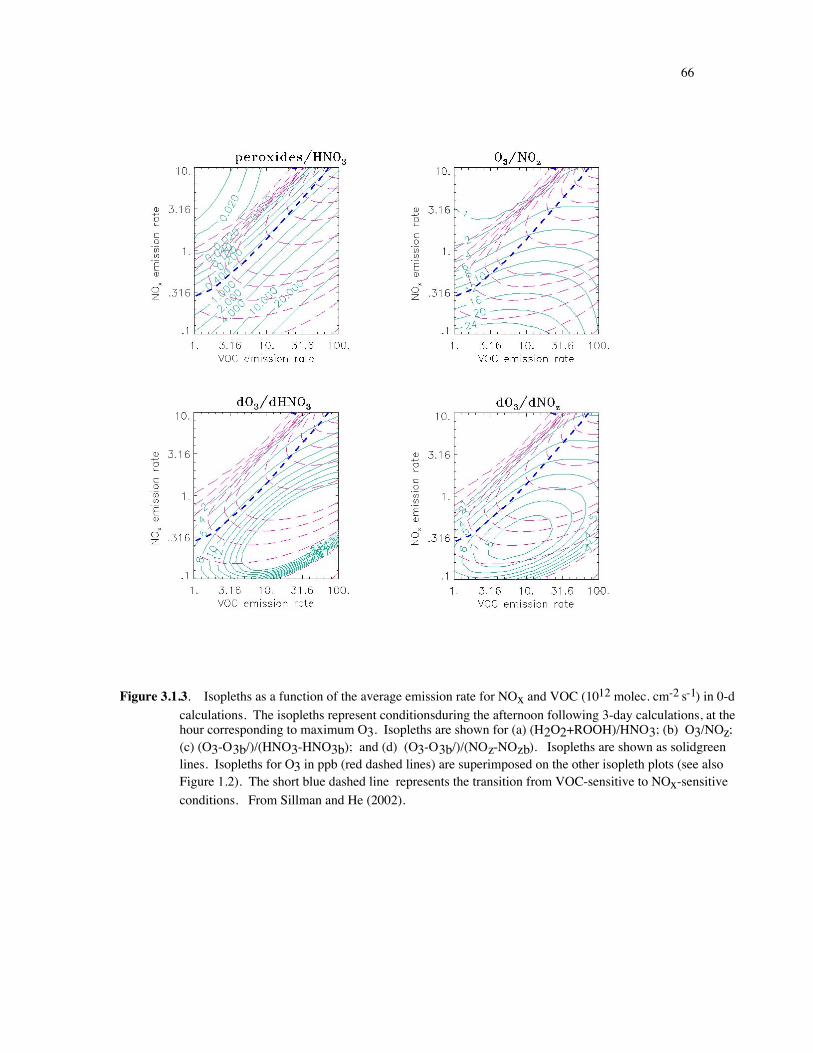
66

Figure 3.1.3. Isopleths as a function of the average emission rate for NOx and VOC (1012 molec. cm-2 s-1) in 0-dcalculations. The isopleths represent conditionsduring the afternoon following 3-day calculations, at thehour corresponding to maximum O3. Isopleths are shown for (a) (H2O2+ROOH)/HNO3; (b) O3/NOz;(c) (O3-O3b/)/(HNO3-HNO3b); and (d) (O3-O3b/)/(NOz-NOzb). Isopleths are shown as solidgreenlines. Isopleths for O3 in ppb (red dashed lines) are superimposed on the other isopleth plots (see alsoFigure 1.2). The short blue dashed line represents the transition from VOC-sensitive to NOx-sensitiveconditions. From Sillman and He (2002).

67

0

4

8

0 100 200 300 400

O3 (ppb)

ratio

(O3-O3b)/HNO3

(O3-O3b)/NOz

Figure 3.1.4. Comparison of the values of (O3-O3b/)/(NOz-NOzb) and (O3-O3b/)/(HNO3-HNO3b) along theNOx-VOC sensitivity transition in isopleth plots based on 0-d calculations. The lines show values alongthe sensitivity transition from 3-day calculations by Sillman and He (2002), shown in Figure 3.1.3. Thepoints show values along the sensitivity transition from 12-hour calculations by Tonnesen and Dennis(2000b).

3.1.5. Contrary evidence

Lu and Chang (1998) and Chock et al. (1999) both published results from 3-d models that sharply contradicted

the original indicator findings. Lu and Chang reported results from a model for the San Joaquin valley (see Table

3.1.1) that included VOC-sensitive conditions for values of O3/NOz as high as 25. Lu and Chang used a definition

of the terms “NOx-sensitive” and “VOC-sensitive” that differed from the definition used by Sillman (1995) (see

Section 3.1.10), but even when the original definition from Sillman (1995) is used, it is apparent that the model

results from Lu and Chang differ from others. The range of values of O3/NOz is 15-30 in the model reported by Lu

68

and Chang (see Figure 3.1.5), as opposed to 5-20 in the models reported previously (Figure 3.1.1). Using Sillman’s

definition, the NOx-VOC transition occurs for O3/NOz equal to 17-20 in the model reported by Lu and Chang, as

opposed to 8-11 in the models shown in Figure 3.1.1.

Chock et al. (1999) also reported contrary results for indicator ratios in a model for Los Angeles (Figure 3.1.3).

As shown in the figure, VOC-sensitive conditions are found for much higher values of O3/NOy (up to 12) and

O3/NOz (up to 20) than in other models, including another model for Los Angeles.

Blanchard and Stoeckenius (2001) compared results from several models (including the original models from

Sillman, 1995 and the model reported by Lu and Chang, 1998). They found that the transition point from NOx- to

VOC-sensitive conditions varied considerably in models for different cities.

The contrary results reported by Lu and Chang are due primarily to different boundary conditions, and can be

corrected by using indicator ratios with the form (O3-O3b)/(NOz-NOzb). In the model by Lu and Chang, the San

Joaquin valley was apparently affected by inflow of air from the model boundary with 75 ppb O3 and less than 1

ppb NOz. This had a significant effect on model results (Sillman et al., 2001). Figure 3.1.5 shows results from the

model by Lu and Chang using the ratio (O3-O3b)/(NOz-NOzb), with background conditions defined for the San

Joaquin valley as described in Section 3.1.10. The ratio does not correlate with NOx- VOC sensitivity as strongly as

in most of the other models, but the approximate range of ratio values (3-7 for VOC-sensitive locations, 5-15 for

NOx-sensitive locations) is comparable to the range of VOC-sensitive values (3-6) and NOx-sensitive values (5-15)

in other models. The model by Lu and Chang also showed correlation patterns for O3 versus NOz that differed

substantially from other models (see Section 3.1.6). The difference in correlation patterns might be used to identify

anomalous results.

Results from the model for Los Angeles reported by Chock et al. still show contradictory results, even for the

ratios (O3-O3b)/(NOy-NOyb). There is no apparent reason for the contrary results, although the model used by

Chock et al. also included varying boundary conditions (from 40 ppb to 80 ppb O3).

Chock et al. (1999) also suggested that plots of the geographical distribution of indicator values and predicted

NOx-sensitive and VOC-sensitive locations would identify inadequacies in indicator ratios that were not visible in

the more direct plots of predicted impact of reduced NOx and VOC versus indicator values. However, as shown in

Figure 3.1.6, the geographical distribution of indicator values and NOx-VOC sensitivity regions suggests the same

69

indicator behavior as can be seen in the standard indicator plots, and in the numerical representation in the

Appendix.

-30

-20

-10

0

10

20

30

40

0 10 20 30 40

O3/NOz .

Ozo

ne r

educ

tion

(ppb

)

reduced NOxreduced VOC -30

-20

-10

0

10

20

30

40

0 5 10 15

(O3-O3b)/(NOz-NOzb) .

Ozo

ne r

educ

tion

(ppb

)


Figure 3.1.5. Contrary evidence from Lu and Chang (1998): Predicted reductions in ozone in response to a 50%reduction in emissions of anthropogenic VOC (crosses), and predicted reductions in response to the samepercent reduction in emissions of anthropogenic NOx (green circles), plotted versus model values forindicator ratios. Results are shown for O3/NOz and (O3-O3b)/(NOz-NOzb) from the model for SanJoaquin reported by Lu and Chang (1998).

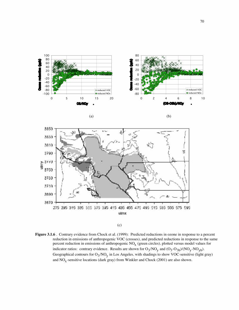
70

-100-80-60-40-20

020406080

100

0 5 10 15 20

O3/NOy .

Ozo

ne r

educ

tion

(ppb

)

reduced VOCreduced NOx -80

-60-40-20

020406080

0 2 4 6 8 10

(O3-O3b)/NOy .

Ozo

ne r

educ

tion

(ppb

)


(a) (b)

(c)

Figure 3.1.6 . Contrary evidence from Chock et al. (1999): Predicted reductions in ozone in response to a percentreduction in emissions of anthropogenic VOC (crosses), and predicted reductions in response to the samepercent reduction in emissions of anthropogenic NOx (green circles), plotted versus model values forindicator ratios: contrary evidence. Results are shown for O3/NOy and (O3-O3b)/(NOy-NOyb).Geographical contours for O3/NOy in Los Angeles, with shadings to show VOC-sensitive (light gray)and NOx-sensitive locations (dark gray) from Winkler and Chock (2001) are also shown.

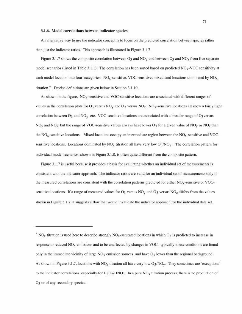
71

3.1.6. Model correlations between indicator species

An alternative way to use the indicator concept is to focus on the predicted correlation between species rather

than just the indicator ratios. This approach is illustrated in Figure 3.1.7.

Figure 3.1.7 shows the composite correlation between O3 and NOy and between O3 and NOz from five separate

model scenarios (listed in Table 3.1.1). The correlation has been sorted based on predicted NOx-VOC sensitivity at

each model location into four categories: NOx-sensitive, VOC-sensitive, mixed, and locations dominated by NOx

titration.* Precise definitions are given below in Section 3.1.10.

As shown in the figure, NOx-sensitive and VOC-sensitive locations are associated with different ranges of

values in the correlation plots for O3 versus NOy and O3 versus NOz. NOx-sensitive locations all show a fairly tight

correlation between O3 and NOy, etc. VOC-sensitive locations are associated with a broader range of O3versus

NOy and NOz, but the range of VOC-sensitive values always have lower O3 for a given value of NOy or NOz than

the NOx-sensitive locations. Mixed locations occupy an intermediate region between the NOx-sensitive and VOC-

sensitive locations. Locations dominated by NOx titration all have very low O3/NOy. The correlation pattern for

individual model scenarios, shown in Figure 3.1.8, is often quite different from the composite pattern.

Figure 3.1.7 is useful because it provides a basis for evaluating whether an individual set of measurements is

consistent with the indicator approach. The indicator ratios are valid for an individual set of measurements only if

the measured correlations are consistent with the correlation patterns predicted for either NOx-sensitive or VOC-

sensitive locations. If a range of measured values for O3 versus NOy and O3 versus NOz differs from the values

shown in Figure 3.1.7, it suggests a flaw that would invalidate the indicator approach for the individual data set.

* NOx titration is used here to describe strongly NOx-saturated locations in which O3 is predicted to increase in

response to reduced NOx emissions and to be unaffected by changes in VOC. typically, these conditions are found

only in the immediate vicinity of large NOx emission sources, and have O3 lower than the regional background.

As shown in Figure 3.1.7, locations with NOx titration all have very low O3/NOy. They sometimes are ‘exceptions’

to the indicator correlations, especially for H2O2/HNO3. In a pure NOx titration process, there is no production of

O3 or of any secondary species.

72

This type of evaluation will identify many situations in which indicator ratios are not valid, due to either erroneous

measurements or to real-world conditions that are inconsistent with the indicator ratios.

In the case study for San Joaquin reported by Lu and Chang (1998), the model correlations between O3 and NOz

differ substantially from the composite predictions of other model scenarios. As shown in Figure 3.1.8, the model

results for San Joaquin show much higher O3 for a given level of NOy and NOz relative to the other model scenarios

shown in Figure 3.1.7 and 3.1.8. The contradictory results for indicator ratios reported by Lu and Chang are also

associated with the difference in the O3-NOz correlation pattern. By examining measured correlations in

comparison with Figures 3.1.7 and 3.1.8, it is possible to evaluate whether a set of measurements is consistent with

the original indicator predictions (Figure 3.1.7) or the contradictory results reported by Lu and Chang (3.1.8).

Equivalent results for measurements are shown in Section 3.1.7.

0

50

100

150

200

250

0 20 40 60 80

NOy (ppb)

Ozo

ne (

ppb)

NOx-sensitiveMixed Hydrocarbon-

sensitive

NOx titration

(a)

Figure 3.1.7 . Correlations for (a) O3 vs. NOy, (b) O3 vs. NOz, (c) O3 vs. HNO3, and (d) total peroxides vs.HNO3 (all in ppb) from the 3-d simulations listed in Table 3.1.1. Each location is classified as NOx-sensitive (green circles), VOC-sensitive (crosses), mixed or with near-zero sensitivity (lavendersquares), and dominated by NOx titration (blue asterisks) based on definitions in the text. From Sillmanand He (2002).

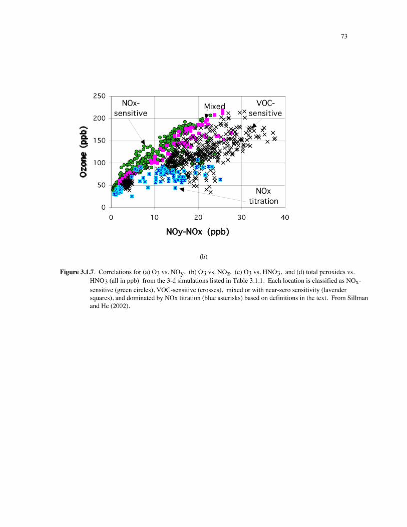
73

0

50

100

150

200

250

0 10 20 30 40

NOy-NOx (ppb)

Ozo

ne (

ppb)

NOx-sensitive

VOC-sensitive

Mixed

NOx titration

(b)

Figure 3.1.7. Correlations for (a) O3 vs. NOy, (b) O3 vs. NOz, (c) O3 vs. HNO3, and (d) total peroxides vs.HNO3 (all in ppb) from the 3-d simulations listed in Table 3.1.1. Each location is classified as NOx-sensitive (green circles), VOC-sensitive (crosses), mixed or with near-zero sensitivity (lavendersquares), and dominated by NOx titration (blue asterisks) based on definitions in the text. From Sillmanand He (2002).

74

0

50

100

150

200

250

0 5 10 15 20 25 30

HNO3 (ppb)

Ozo

ne (

ppb)

NOx-sensitive Mixed VOCsensitive

NOx titration

(c)

Figure 3.1.7. Correlations for (a) O3 vs. NOy, (b) O3 vs. NOz, (c) O3 vs. HNO3, and (d) total peroxides vs.HNO3 (all in ppb) from the 3-d simulations listed in Table 3.1.1. Each location is classified as NOx-sensitive (green circles), VOC-sensitive (crosses), mixed or with near-zero sensitivity (lavendersquares), and dominated by NOx titration (blue asterisks) based on definitions in the text. From Sillmanand He (2002).

75

0

2

4

6

8

10

12

14

0 5 10 15 20 25 30

HNO3 (ppb)

pero

xide

s (p

pb)

(d)

Figure 3.1.7 . Correlations for (a) O3 vs. NOy, (b) O3 vs. NOz, (c) O3 vs. HNO3, and (d) total peroxides vs.HNO3 (all in ppb) from the 3-d simulations listed in Table 3.1.1. Each location is classified as NOx-sensitive (green circles), VOC-sensitive (crosses), mixed or with near-zero sensitivity (lavendersquares), and dominated by NOx titration (blue asterisks) based on definitions in the text. From Sillmanand He (2002).

76

0

50

100

150

200

250

0 20 40 60 80

NOy (ppb) .

Ozon

e (p

pb)


sensitive

NOx titration

Los Angeles

0

50

100

150

200

250

0 20 40 60 80

NOy (ppb) .

Ozon

e (p

pb)


sensitive

Northeast

0

50

100

150

200

250

0 20 40 60 80

NOy (ppb) .

Ozon

e (p

pb)

NOx-sens.MixedVOC-sens.

Atlanta

0

50

100

150

200

250

0 20 40 60 80

NOy (ppb) .

Ozon

e (p

pb)


sensitive

Lake Michigan

0

50

100

150

200

250

0 20 40 60 80

NOy (ppb) .

Ozon

e (p

pb)

NOx-sens.mixedVOC-sens.NOx titr.

Nashville

0

50

100

150

200

250

0 20 40 60 80

NOy (ppb) .

Ozon

e (p

pb)

San Joaquin (Lu and Chang)

Figure 3.1.8. Correlations for O3 vs. NOy in ppb from individual 3-d simulations listed in Table 3.1.1. Eachlocation is classified as NOx-sensitive (green circles), VOC-sensitive (crosses), mixed or with near-zerosensitivity (lavender squares), and dominated by NOx titration (blue asterisks) based on definitions in thetext. Models are (a) Los Angeles (Godowitch), (b) Lake Michigan, (c) northeast corridor,(d) Nashville, (e) Atlanta, and (f) San Joaquin (Lu and Chang).

77

3.1.7. Results from ambient measurements

Figure 3.1.9 shows correlations between measured O3 and NOy and between O3 and NOy during events in four

metropolitan areas: Atlanta (August 10, 1992); Nashville (July 15, 1995); Paris (July 17, 1999); and Los Angeles

(August 27, 1988).

These correlation patterns show substantial differences between urban areas, which might be interpreted as

evidence of different NOx-VOC sensitivity. Comparing with Figure 3.1.6, these patterns would be interpreted as

suggestive of NOx-sensitive conditions in Atlanta, mixed sensitivity in Nashville and Paris, and strongly VOC-

sensitive conditions in Los Angeles.

Correlation patterns of O3 versus NOz in rural areas also show variations, which have been interpreted as

representative of differences between NOx-sensitive and VOC-sensitive conditions (Jacob et al., 1995; Hirsh et al.,

1996). However, since rural areas usually have NOx-sensitive chemistry, correlations among these species from

research-grade measurements in rural areas provide an important test for the accuracy of the predicted correlation

patterns shown in Figure 3.1.7 and Figure 3.1.8.

Figure 3.1.10 shows results from research-grade field measurements in rural areas in the eastern and southern

U.S. These correlations (between O3 and NOy and between Ox and NOz) are consistent with the model correlation

for NOx-sensitive conditions.

More detailed information can be obtained in cases where measured H2O2 or total peroxides are available. As

shown in Figure 3.1.11, 3-d models and measurements both predict a strong correlation between O3 and the sum

(2H2O2+NOz). This correlation represents an important evaluation of the indicator approach because the species

involved are all major components of the indicator ratios.

The correlation between O3 and (2H2O2+NOz) is important because discrepancies between model and measured

correlations would suggest errors that would invalidate the indicator method. Unlike the proposed indicator ratios,

O3 and (2H2O2+NOz) show a similar linear correlation in both NOx-sensitive and VOC-sensitive locations. This

means that any discrepancy between model and measured correlations suggests errors that are unrelated to predicted

NOx-VOC sensitivity. These errors would cast doubt on the relation between indicator ratios and NOx-VOC

sensitivity as predicted by models. Alternatively, a good agreement between models and measurements for O3

78

versus (2H2O2+NOz) can provide evidence that many uncertain features of the model (ozone production

efficiencies, dry deposition rates, etc.) are consistent with measured values.

0

50

100

150

200

250

0 20 40 60 80

NOy (ppb)

Ozo

ne (

ppb)

AtlantaNashvilleParisLos Ang.

Figure 3.1.9. Measured correlation between O3 and NOz in Atlanta (green circles), Nashville (pink dashes), Paris(blue diamonds) and Los Angeles (crosses) for the events of August 10, 1992 (Atlanta); July 13, 1995(Nashville); July 17, 1999 (Paris); and August 28, 1987 (Los Angeles), from measurements reported bySillman et al. (1995, 1997, 1998, 2002).

79

(a) O3 versus NOy at six rural sites (Trainer et al., 1993)

(b) O3 versus NOz at six rural sites (Trainer et al., 1993)

Figure 3.1.10. Measured O3 versus NOy, O3 versus NOz and O3 versus PAN. The figures show (a) O3 versusNOy at six rural sites in the eastern U.S. (Trainer et al., 1993); (b) O3 versus NOz at six rural sites in theU.S. (Trainer et al., 1993); (c) O3 versus NOz for two week-long time periods at a rural site inMassachusetts with different correlation patterns (Hirsch et al., 1996); (d) O3 versus NOz at rural sitesin Tennessee (Olszyna et al., 1998); and (e) O3 versus PAN at rural sites in Tennessee (Roberts et al.,1998).

80

(c) O3 versus NOz in rural Massachusetts (Hirsch et al., 1996)

(d) O3 versus NOz at a site in Tennessee (Olszyna et al., 1998)

Figure 3.1.10 . Measured O3 versus NOy, O3 versus NOz and O3 versus PAN. The figures show (a) O3 versusNOy at six rural sites in the eastern U.S. (Trainer et al., 1993); (b) O3 versus NOz at six rural sites in theU.S. (Trainer et al., 1993); (c) O3 versus NOz for two week-long time periods at a rural site inMassachusetts with different correlation patterns (Hirsch et al., 1996); (d) O3 versus NOz at rural sitesin Tennessee (Olszyna et al., 1998); and (e) O3 versus PAN at rural sites in Tennessee (Roberts et al.,1998).

81

0

20

40

60

80

100

120

140

160

0 10 20 30 40

2H2O2+NOz (ppb) .

Ozo

ne (

ppb)

NOx-sens.mixedVOC-sens.NOx titr.measured

Figure 3.1.11. Measured correlation between O3 and the sum 2H2O2+NOz (ppb) in Nashville (blue diamonds),compared with model results. Each model location is classified as NOx-sensitive (green circles), VOC-sensitive (crosses), mixed or with near-zero sensitivity (lavender squares), and dominated by NOxtitration (blue asterisks) based on definitions in the text. The model and measurements are from Sillmanet al. (1998).

82

3.1.8. Model evaluations with measured indicator species: a method for regulatory use

The most promising use of the indicator concept involves the use of measured species identified as NOx-VOC

indicators to evaluate results from 3-d models.

Evaluations of model performance using measured indicator species have been reported for Atlanta, Nashville,

Los Angeles and Paris (Sillman et al., 1995, 1997, 1998, 2002b). In each of these evaluations, measured

correlations between O3 and NOy and between O3 and NOz were compared with predicted correlations from a

series of model scenarios. The model scenarios included cases with NOx and VOC emissions modified from the

initial rates derived from emission inventories and with modified wind speeds and mixing heights. Due to the

modified emissions, the model scenarios also included cases with different NOx-VOC predictions (see Figure 1.2

and Section 1.4 above). These scenarios provide a test to see whether the model-measurement evaluation can

distinguish between alternatives with different control predictions.

Figure 3.1.12 shows four model-measurement comparisons that illustrate different types of results. In the case

for Atlanta (Figure 3.1.12a), model O3 versus NOy shows a correlation that largely agrees with measured

correlation, but only when the model predicts NOx-sensitive conditions. When the model predicts VOC-sensitive

conditions, especially for high ozone, the model Ox and NOy differ from the measured correlation. The model

values of the ratio O3/NOy associated with VOC-sensitive conditions are also much lower than measured values.

This pattern strongly suggests that the model (which used the BEIS1 inventory) was biased in its NOx-VOC control

predictions and overestimated the benefits of reducedVOC.

In the case for Los Angeles (Figure 3.1.12b) the model O3 versus NOz agrees with the measured correlation

only when the model predicts VOC-sensitive conditions. When the model predicts NOx-sensitive conditions it has

O3 and NOz that is higher than measured values. There is some uncertainty here because the highest measured O3

is not that far removed from the model NOxsensitive region. However, the general comparison suggests that the

model (which had VOC emissions much higher than inventory values) overestimated the possible benefits of

reduced NOx.

In the case for Nashville (Figure 3.1.12c) there is a good agreement between model and measured O3 and NOy,

suggesting that the model provides an unbiased estimate of the impacts of reduced NOx and VOC emissions.

83

In the case for Paris (Figure 3.1.12d) there is a disagreement between models and measurements throughout the

model domain. This disagreement is not related to model NOx-VOC predictions. The same disagreement appears

for both NOx-sensitive and VOC-sensitive conditions. In this case, the measured O3 versus NOz cannot be

interpreted as evidence concerning NOx-VOC sensitivity. The cause of the model-measurement discrepancy is

unknown, but there is a high likelihood that the cause (e.g. rapid deposition of HNO3, conversion to unmeasured

aerosol nitrate, erroneous measurements, etc.) would invalidate the use of measured values as NOx-VOC indicators.

These comparisons have been chosen to illustrate the different patterns that appear and do not represent a

complete analysis of either city.

If indicator ratios are to be used for regulatory purposes, protocols are needed to distinguish between the three

types of model-measurement comparison shown here.

84

0

20

40

60

80

100

120

140

160

180

200

0 10 20 30 40

NOy (ppb) .

Ozo

ne (

ppb)

(a) Atlanta, August 10, 1992

0

50

100

150

200

250

0 20 40 60 80

NOz (ppb) .

Ozo

ne (

ppb)

(b) Los Angeles, August 27, 1987

Figure 3.1.12. Measured correlation between O3 and NOy and between O3 and NOz (ppb) (blue diamonds),compared with model results. Each model location is classified as NOx-sensitive (green circles), VOC-sensitive (crosses), mixed or with near-zero sensitivity (lavender squares), and dominated by NOxtitration (blue asterisks) based on definitions in the text. Cases are shown for (a) Atlanta, (b) LosAngeles, (c) Nashville, and (d) Paris, from Sillman et al. (1995, 1997, 1998, 2002).

85

0

20

40

60

80

100

120

140

160

0 10 20 30 40

NOy-NOx (ppb) .

Ozo

ne (

ppb)

(c) Nashville, July 13, 1995

20

40

60

80

100

120

140

0 10 20 30

NOz

Ozo

ne

NOx-sens.mixedVOC-sens.Measured

(d) Paris, July 18, 1999

Figure 3.1.12. Measured correlation between O3 and NOy and between O3 and NOz (ppb) (blue diamonds),compared with model results. Each model location is classified as NOx-sensitive (green circles), VOC-sensitive (crosses), mixed or with near-zero sensitivity (lavender squares), and dominated by NOxtitration (blue asterisks) based on definitions in the text. Cases are shown for (a) Atlanta, (b) LosAngeles, (c) Nashville, and (d) Paris, from Sillman et al. (1995, 1997, 1998, 2002).

86

3.1.9. Results for O3 versus PAN: possible impact of erroneous measurements

A major issue for NOx-VOC indicators concerns the accuracy of available measurements.

Measured NOy and NOz can only be used in indicator ratios and correlations if the measurements include HNO3.

The information in these ratios that relates to NOx-VOC sensitivity is contained primarily in HNO3. The other

components of NOz, including PAN and other organic nitrate, are not related to O3-NOx-VOC sensitivity. Ratios

such as O3/PAN are not correlated with NOx-VOC sensitivity in models (Tonnesen and Dennis, 2000b).

This issue is important because HNO3 is sometimes lost along the inlet tubes when NOy is measured (Parrish et

al., 2000; McClenny et al., 2000). If HNO3 were missing from measured NOy, then the remaining measurement

(NOx+organic nitrates) could not be used to evaluate NOx-VOC sensitivity.

NOx measurements that use chemilluminescence also sometimes respond to PAN in addition to NOx (Logan,

1989), McClenny, 2000). This would affect the accuracy of NOz, which is measured as the difference between

NOy and NOx.

McClenny (2000) recommended changes in the PAMS network that would insure the accuracy of measured NOy

and NOx. Williams et al. (1998) also reported good results from an intercomparison of NOy instruments. However

it is also important to evaluate individual measurement sets to determine whether these types of errors occur. Luke

et al. (1998) reported incidences of apparent errors in individual measurements of NOy.

Figure 3.1.13 shows the correlation between O3 and organic nitrates (defined as NOy-NOx-HNO3) for the five

models shown in figure 3.1.7. In this figure a very similar correlation pattern is shown for both NOx-sensitive and

VOC-sensitive locations.

The correlation between O3 and organic nitrates is also distinctly different from the predicted correlation for Ox

versus NOz in Figure 3.1.7. Thus, comparison of measured O3 versus NOz with the predicted correlation for O3

versus organic nitrates can be used as a diagnostic test for this type of measurement error.

The model correlation between O3 and organic nitrates is generally consistent with ambient measurements of O3

versus PAN (Figure 3.1.14).

87

0

50

100

150

200

250

0 10 20 30 40

organic nitrates (ppb) .

Ozo

ne (

ppb)

NOx-sensmixed sensVOC-sensNOx-titration

Figure 3.1.13. Correlations for organic nitrates (defined as NOy-NOx-HNO3, in ppb) from the 3-d simulationslisted in Table 3.1.1. Each location is classified as NOx-sensitive (green circles), VOC-sensitive(crosses), mixed or with near-zero sensitivity (lavender squares), and dominated by NOx titration (blueasterisks) based on definitions in the text.

88

Figure 3.1.14. Measured O3 (ppb) versus PAN (ppt) at in Tennessee, including (a) aircraft measurements, and (b, candd) suburban sites near Nashville (Roberts et al., 1998).

89

3.1.10. Supplemental topic: Defining O3-NOx-VOC sensitivity

As described in Section 2.2, there are two standard ways to define O3-NOx-VOC sensitivity: relative impact of

reduced NOx versus reduced VOC; and NOx benefits versus disbenefits. The results reported by Sillman were all

based on the first definition. Tonnesen and Dennis (2001b) reported results for both definitions and found small but

significant differences in the indicator transition values. Typically, transition values were 15% lower for NOx

benefits versus disbenefits than for the relative impact of NOx versus VOC. In each case, NOx-VOC sensitivity was

defined relative to changes in emissions of anthropogenic NOx and VOC ranging from 25% to 50%. A different

response to changed NOx and VOC can be expected if much higher percent reductions were used (Schere and

Roselle, 1995).

The correlation plots (Figures 3.1.7, etc.) all used the following definition of sensitivity, applied to specific

model locations relative to predicted changes in O3 at the same time and location in model scenarios with reduced

NOx and VOC:

NOx-sensitive: O3 in model scenarios with reduced NOx is lower than O3 in the base case by at least 5 ppb, and

lower then in model scenarios with the same percent reduction in VOC by at least 5 ppb.

VOC-sensitive: O3 in the scenario with reduced VOC is lower than O3 in both the base case and in the scenario

with reduced NOx by at least 5 ppb.

Mixed: The scenarios with reduced NOx and reduced VOC have O3 within 5 ppb of each other, and both have O3

lower than in the base case by at least 5 ppb.

NOx-titration: O3 in the scenario with reduced NOx is larger than O3 in the base case by at least 5 ppb, and O3 in

the simulation with reduced VOC is not lower by 5 ppb or more relative to the base case.

All other locations are viewed as insensitive to NOx and VOC in the context of the model domain. These

typically represent locations with O3 dominated by transport from outside the model boundary rather than calculated

photochemical production.

The locations dominated by NOx-titration are usually near large sources of NO. These locations typically have

relatively low O3, and O3 has been affected primarily by the reaction O3+NOÆNO2 in the presence of directly

emitted NO rather than by ozone production chemistry. These locations always have very low O3/NOy and

O3/NOx, and are therefore easy to identify.

90

3.1.11. Supplemental topic: Determining background values

Background concentrations represent an important uncertainty for indicator ratios such as (O3-O3b)/(NOy-

NOyb). Background concentrations in models can be identified based on boundary conditions, but for ambient

conditions the background is less clear. In evaluating model results it is necessary to determine background

concentrations in a way that is directly comparable to the background that can be determined from a measured data

set.

Sillman and He (2002) adopted the following procedure for boundary conditions. They assumed that modeling

was to be done for a metropolitan area with a network of surface measurements (including the surrounding rural

area). They defined background concentrations as equal to the value at the measurement site that reported minimum

NOy, using measurements at the same hour (in the afternoon) as the O3 they intended to analyze. Although

somewhat arbitrary, this definition would allow background concentrations to be determined from surface

measurements alone and avoided the need to make assumptions about the upwind origin of air. The equivalent

background concentration from model scenarios was found by identifying the model surface grid with minimum

NOy within the metropolitan area.

An additional problem with model interpretation concerned the interpretation of model sensitivity predictions in

when the background concentrations determined in this way were different from the model boundary conditions.

For example, in an examined case for Atlanta (using the model listed in Table 3.1.1), the model boundary O3 was 55

ppb and the background O3 determined by the above method was 74 ppb. In this case, the background O3 already

included significant O3 production and the model sensitivity runs included changed background O3. In this case,

consistent results were found only if the predicted impact of reduced NOx and VOC at the background location were

subtracted from the predicted impact of reduced NOx and VOC elsewhere in the model domain. With sensitivity

adjusted in this way, model correlations between indicator ratios and NOx-VOC sensitivity were identical with the

derived background concentrations as they would be with background concentrations set equal to the model

boundary values.

Olszyna et al. (1994) determined background O3 in connection with smog production algorithms (Section 3.2) by

extrapolating the observed linear correlation of O3 with NOz to find the O3 that would be associated with zero NOz.

91

This method may not be applicable in many urban cases, because the correlation between O3 and NOz is not always

linear.

In regional-scale analyses, model background conditions are often set based on typical conditions in the clean

troposphere outside the borders of the U.S. (including conditions over the Atlantic and Pacific Oceans and sparsely

populated parts of Canada). In these cases there may be no appropriate measurements to identify the regional

background, but background conditions may be reasonably assumed to be equal to the model background.

Conditions in the clean troposphere in summer are typically 30-40 ppb O3, 0.1 ppb NOx or lower, and less than 1

ppb NOy, with little day-to-day variation. (Logan, 1988; Carroll et al., 1990; Chin et al., 1994).

3.1.12. Supplemental topic: Radical chemistry and O3-NO3-VOC sensitivity

The relation between the ratio O3/NOz and NOx-VOC sensitivity can be understood intuitively in terms of the

well-known relationship between NOx-VOC sensitivity and VOC/NOx ratios. The main reactions associated with

ozone formation are summarized in Table 3.1.2. The ozone production sequence is initiated by reaction of various

VOC and CO with OH (R1 in Table 3.1.2). The resulting RO2 and HO2 radicals go on to react with NO (R2 and

R3), and the resulting NO2 photolyzes to produce ozone. Because the reaction of VOC with OH is the rate-limiting

step for the sequence it is possible to regard the rate of ozone production as proportional to the summed rate of

VOC+OH (R1). This rate may be compared to the rate of formation of nitric acid (NO2+OH, R10). Comparing the

rates of reactions R1 and R10, it is possible to express the ratio of the rate of ozone production to that of nitric acid

as follows:

PO3PHNO3

=kOHi[VOCi ]iÂ

kOHn[NO2 ] (3.1.1)

where VOCi represents individual VOC species and kOHi represents the rate constant for the reaction of the

individual VOC with OH. The ratio on the right side of Equation 3.1.1 is the familiar ratio of reactivity-weighted

VOC (abbreviated rVOC) to NOx, normalized relative to the rate constant for the reaction of NO2 with OH (kOHn).

As will be discussed in Section 3.3, the ratio of reactivity-weighted VOC to NOx is closely associated with the NOx-

VOC sensitivity of instantaneous ozone production.

92

The ratios O3/NOz and O3/HNO3 could therefore be regarded as surrogates for the sum of the ratio of reactivity-

weighted VOC to NOx over time.

Photochemical uncertainties include the following: variations in the rate of ozone production per VOC+OH

reaction for individual VOC and for different photochemical mechanisms; rates of formation of organic nitrates

(which affect O3/NOz); impact of nighttime formation of HNO3 via aerosol reactions; and the deposition rate of

HNO3.

Sillman (1995), Kleinman et al. (1997) and Tonnesen and Dennis (2000a) presented more detailed analyses of

the chemistry of O3-NOx-VOC sensitivity, based on the chemistry of odd hydrogen radicals. A summary is

presented here. The odd hydrogen radicals include OH, HO2 and RO2 (including CH3O2, CH3CO3, and analogous

radicals). The chemistry of these species has a large influence on the ozone formation process.

Tonnesen and Dennis (2001) presented the cycle of odd hydrogen in terms of three stages: chain initiation, or

radical sources (abbreviated as SH in publications by Sillman et al. and as Q in the work of Kleinman et al.); chain

propagation, or interconversion among OH, HO2 and RO2; and chain termination, or radical sinks. Chain

initiation occurs through the photolysis of ozone (R5), photolysis of HCHO and other secondary VOC (R6), and

reaction of alkenes with O3 (R7). Chain propagation occurs through reactions of CO and VOC with OH (R1) and

reactions of HO2 and RO2 with NO (R2 and R3), each of which is part of the ozone formation sequence. Chain

termination occurs through three processes: formation of peroxides (R8 and R9); formation of nitric acid (R10);

and formation of PAN and other organic nitrates (R11).

It is easy to show that ozone formation will have NOx-sensitive characteristics whenever peroxides represent the

dominant odd hydrogen sink and VOC-sensitive characteristics whenever nitric acid represents the dominant sink.

Because odd hydrogen radicals are short-lived, the sources and sinks must be in steady state:

SH = 2Pperox + PHNO3 + PorgN (3.1.2)

If peroxides represent the dominant sink, then the concentration of HO2 and RO2 (controlled by SH and the

quadratic loss rates through R8 and R9) is largely independent of NOx and VOC, and the ozone formation rate (via

HO2+NO and RO2+NO, R2 and R3) increases with increasing NOx. If nitric acid represents the dominant sink,

then OH (controlled by SH and removal through OH+NO2, R10) decreases with increasing NOx and the ozone

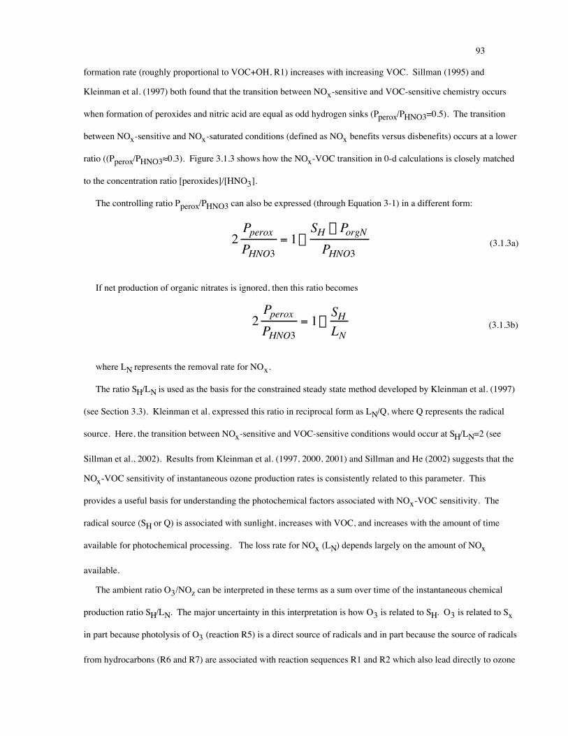
93

formation rate (roughly proportional to VOC+OH, R1) increases with increasing VOC. Sillman (1995) and

Kleinman et al. (1997) both found that the transition between NOx-sensitive and VOC-sensitive chemistry occurs

when formation of peroxides and nitric acid are equal as odd hydrogen sinks (Pperox/PHNO3=0.5). The transition

between NOx-sensitive and NOx-saturated conditions (defined as NOx benefits versus disbenefits) occurs at a lower

ratio ((Pperox/PHNO3≈0.3). Figure 3.1.3 shows how the NOx-VOC transition in 0-d calculations is closely matched

to the concentration ratio [peroxides]/[HNO3].

The controlling ratio Pperox/PHNO3 can also be expressed (through Equation 3-1) in a different form:

2Pperox

PHNO3= 1-

SH - PorgN

PHNO3 (3.1.3a)

If net production of organic nitrates is ignored, then this ratio becomes

2Pperox

PHNO3= 1-

SHLN

(3.1.3b)

where LN represents the removal rate for NOx.

The ratio SH/LN is used as the basis for the constrained steady state method developed by Kleinman et al. (1997)

(see Section 3.3). Kleinman et al. expressed this ratio in reciprocal form as LN/Q, where Q represents the radical

source. Here, the transition between NOx-sensitive and VOC-sensitive conditions would occur at SH/LN=2 (see

Sillman et al., 2002). Results from Kleinman et al. (1997, 2000, 2001) and Sillman and He (2002) suggests that the

NOx-VOC sensitivity of instantaneous ozone production rates is consistently related to this parameter. This

provides a useful basis for understanding the photochemical factors associated with NOx-VOC sensitivity. The

radical source (SH or Q) is associated with sunlight, increases with VOC, and increases with the amount of time

available for photochemical processing. The loss rate for NOx (LN) depends largely on the amount of NOx

available.

The ambient ratio O3/NOz can be interpreted in these terms as a sum over time of the instantaneous chemical

production ratio SH/LN. The major uncertainty in this interpretation is how O3 is related to SH. O3 is related to Sx

in part because photolysis of O3 (reaction R5) is a direct source of radicals and in part because the source of radicals

from hydrocarbons (R6 and R7) are associated with reaction sequences R1 and R2 which also lead directly to ozone

94

formation. Since photolysis of O3 is usually an important source of odd hydrogen, the relation between O3 and SH

should also vary depending on the extent of photochemical aging.

In the original 3-d models by Sillman (1995) it was found that the NOx-VOC transition occurs at a lower value of

O3/NOz early in the day, possibly due to the influence of photochemical aging. The ratio O3/NOz performs

somewhat better as a NOx-VOC indicator because it represents a ratio of reaction products (O3/NOz) modified by a

ratio related to photochemical aging (NOz/NOy).

95

Table 3.1.2

Chemical reactions relevant to ozone formation and odd hydrogen radicals

_____________________________________________________________________________________________

Ozone formation sequence:

R1. VOC+OHÆRO2 R1a. CO+OHÆHO2 R2. RO2+NOÆNO2+HO2+intermediate VOCR3. HO2+NOÆOH+NO2 R4. NO2 + hn O2æ Æ æ NO + O3

Sources of odd hydrogen radicals (chain initiation):

R5. O3 + hnH2O

æ Æ æ æ 2OH R6. HCHO+hnÆ2HO2+CO R6a. other aldehydes+hnÆHO2, RO2, RCO3 R7. Olefin+O3Æ OH, HO2, intermediate VOC

Sinks for odd hydrogen (chain termination):

R8. HO2+HO2ÆH2O2 R9. HO2+RO2ÆROOH R10. OH+NO2ÆHNO3 R11. CH3CO3 + NO2 ´ PAN (net formation)

_____________________________________________________________________________________________

96

3.2 SMOG PRODUCTION ALGORITHMS (EXTENT OF REACTION PARAMETERS)


• Smog production algorithms (also known as extent-of-reaction parameters) refers to a series of parameters

developed by Johnson (1984), Hess et al. (1992a, b and c), Chang et al. (1997) and Blanchard et al. (1999,

2000) to analyze O3-NOx-VOC sensitivity. The parameters all involve measured O3, NOx and/or NOy.

• The distinctive feature of smog production algorithms (as opposed to NOx-VOC indicators) is that the smog

algorithms are derived from smog chamber experiments, whereas the NOx-VOC indicators discussed in Section

3.1 (often involving the same species) were derived from 3-d photochemical models.

• The smog production algorithms are based on the concept that the rate of ozone production in fresh emissions is

always VOC-sensitive, and that conditions become NOx-sensitive when the initial NOx concentration of the air

mass has reacted away. VOC-sensitive versus NOx-sensitive conditions can be diagnosed through parameters

that represent the extent of reaction.

• The parameter (1-NOx/NOy) has been widely used by researchers to represent extent of reaction or

photochemical aging (e.g. Trainer et al., 1993; Olszyna et al., 1994). Here, the term “smog production

algorithms” will be used to refer to the specific theory that extent of reaction may be used to identify NOx-VOC

sensitivity.

• Several forms of smog production algorithms have been developed. The major alternatives are based on the

ratios (O3-O3b)/NOy, NOx/NOy and (O3-O3b)/NOx.

• The smog production algorithms were developed from chamber experiments that represent an initial large

concentration of VOC and NOx, followed by photochemical evolution without additional emissions. It is

unclear whether the relationships derived from these experiments are applicable to ambient conditions, which

have a complex pattern of continuous anthropogenic and biogenic emissions.

• The smog algorithms have been widely used to evaluate NOx-VOC chemistry in the U.S., and have included

evaluations of data over several years rather than just for individual events. These evaluations have consisted

primarily of deriving the measured smog production parameters and interpreting them as evidence for NOx-

VOC sensitivity. There has been very little interpretation of measured data to determine the viability of the

method.

97

• Evaluation of smog production parameters in comparison with NOx-VOC predictions in 3-d models has yielded

mixed results. The smog production parameters based on (O3-O3b)/NOy are generally correlated with NOx-

VOC sensitivity in models. Parameters based on NOx/NOy and (O3-O3b)/NOx show a much worse correlation.

• The smog production parameters recommended by Chang et al. (1997) and Blanchard et al. (1999) have the

form (O3-O3b)/NOya where the exponent a is 0.5 or 0.67. Model results suggest that simpler ratio,

(O3-O3b)/NOy, is correlated more closely with NOx-VOC sensitivity.

• Smog production algorithms assume zero deposition. A rough calculation is added to represent deposition.


• Smog production algorithms appear to give meaningful results primarily in situations with strongly VOC-

sensitive chemistry. They are less successful at distinguishing moderately VOC-sensitive conditions from NOx-

sensitive conditions.

• Smog production algorithms based on measured NOx/NOy or O3/NOx are unreliable and should not be used.

• The conclusions given in Section 3.1.2 for NOx-VOC indicators also generally apply for smog production

algorithms. Smog production algorithms require accurate measurement of NOy; they should be developed in

the form of predicted species correlations rather than just used as a “rule of thumb”; and their use should be

expanded to include a measurement-based evaluation of model predictions.

3.2.3. The smog production concept: results from smog chambers

The smog production concept, originally developed by Johnson (1984) and originally presented in scientific

literature by Hess et al. (1992a, 1992b, 1992c) was based on a series of observations in smog chamber experiments.

In these experiments it was found that the amount of smog produced (SP, defined as (O3-NO)-(O3-NO)background)

increased linearly with time, where time elapsed was measured as the integrated sum of incident sunlight (expressed

as ∫ jNO2dt, where jNO2 represents the NOx photolysis rate). The amount of smog produced in the experiments

increased linearly up to the point where all the initial NOx had reacted away. After that the amount of smog

produced remained constant. Johnson and Hess et al. found that the final (maximum) amount of smog produced

depended entirely on the initial amount of NOx in the experiment and was independent of VOC. They also found

that the rate of smog production during the initial phase depended on the amount of VOC.

98

Johnson interpreted as evidence that NOx-VOC chemistry could be analyzed in terms of the extent of reaction of

ambient NOx. As a mixture of freshly emitted NOx and VOC began producing ozone, the rate of ozone formation

was limited by the availability of sunlight, expressed as the time integrated sum of jNO2. This “light-limited”

regime corresponds to VOC-sensitive or NOx-saturated conditions. After the initial NOx has reacted to the point

where the remaining NOx is very low the mixture reaches the NOx-limited regime, and additional smog formation is

possible only if more NOx is added. NOx-sensitive conditions thus correspond to a situation in which the available

NOx has reacted to completion (high extent of reaction), whereas VOC-sensitive conditions correspond to situations

in which the NOx has not yet reacted completely (low extent of reaction).

In subsequent experiments it was found that additional injection of either VOC or NOx produced results that

were consistent with this analysis of light-limited and NOx-limited regimes. A subsequent injection of NOx would

not affect the rate of smog production, but would allow smog formation to continue to a higher final total amount. A

subsequent injection of VOC would cause the rate of smog production to increase, but it would not increase the final

amount of smog, and would not cause a further increase if the initial NOx had been reacted to completion. These

experiments are illustrated in Figure 3.2.1. As shown in the figure, these patterns were reproduced in calculations

using the CB-IV photochemical mechanism. Similar patterns were also found in 0-d calculations (Blanchard et al.,

1999).

Based on these results, it was proposed that ozone chemistry could be evaluated in terms of an extent-of-reaction

parameter, defined as:

Extent =SP

SPmax(3.2.1)

where SPmax represents the maximum possible smog production if all the available NOx were processed. SPx

was viewed as a function of the initial NOx (NOx(i)) available in the air mass, which would be approximated from

measurements. The subsequent smog production algorithms were all based on this form.

Johnson’s original algorithm used ambient NOy to represent SPmax. The resulting extent parameter from

Johnson (1990) was

99

ExtentJ =O3 - O3b - NO + 0.9NOy

4.09NOy(3.2.2)

This extent parameter has an obvious similarity to the indicator ratio (O3-O3b)/(NOy-NOyb), developed much

later by Sillman (1995). The ratio 4.09 represents the rate of ozone production per NOx, assuming that all NOx has

reacted to completion. The implied result is that ozone production efficiency per NOx always has a constant value

(4.09) after the emitted NOx has reacted completely.

Chang et al. (1997) and Blanchard et al. (1999, 2000) both generated modified forms of the original extent

parameter. Blanchard et al. found that the final amount of ozone produced in smog chamber experiments (SPmax)

was not a exact linear function of initial NOx (NOx(i)) and that SPmax is better represented by [NOx(i)]a, with a

estimated at 0.5 by Chang and 0.67 by Blanchard, rather than by [NOx(i)]. The correlation between SPmax and

NOx(i) reported by Blanchard is shown in Figure 3.2.2. Blanchard et al also generated extent formulas based on

NOx/NOy, and O3/NOx, in addition to a modified version of the original formula based on O3/NOy. The extent

parameters proposed by Blanchard et al. (1999) were as follows. The parameter based on O3/NOy used the

following format:

ExtentB1 =O3 + D[O3] - O3b - NO + 0.95NOx (i)

19(NOx (i))0.67 (3.2.3a)

where NOx(i) is determined from ambient NOy:

NOx (i) = NOy + D[NOy ] (3.2.3b)

here, all species concentrations refer to ambient measurements at the location for which Ox-NOx-VOC

sensitivity is being investigated. As was the case for NOx-VOC indicators, the smog production formulas provide

evidence about NOx-VOC sensitivity of ozone concentrations (not instantaneous production rates), only at the exact

time and place of the measured values. D[O3] and D[NOy] represent estimates for loss of O3 and NOy through

deposition as the air mass has traveled from the emission source to the measurement site. Deposition is not included

in any of the smog production formulas. Blanchard et al. recommend that deposition rates be calculated for a time

interval beginning at sunrise and ending at the (afternoon) hour (t) being evaluated, as follows:

100

D[O3 ] =36 vd (t )O3(t )

t=0600tÂ

z(t) (3.2.4a)

where vd(t) represents the time-varying deposition velocity in cm s-1 and z(t) represents the mixing height (m) at

the hour being evaluated. They recommend that deposition velocity be approximated using a formula for diurnal

variation:

vd (t) = N + Asin 2p(t - 0600)2800 (3.2.4b)

with the above formula applied for daylight hours only, and the minimum diurnal deposition velocity (N) used at

night. Deposition of NOy would be determined in similar fashion. They recommend using N=0.2 cm s-1 and A=0.3

cm s-1 for both O3 and NOy.

The smog production algorithm based on NOx/NOy is:

ExtentB2 = 1 -NOx

NOx(i)

È

Î Í Í

˘

˚ ˙ ˙

0.67

(3.2.5)

where NOx(i) is determined from measured NOy as in Equation 3.2.3b.

The smog production algorithm based on O3/NOx, referred to here as ExtentB3, uses Equation 3.2.3a with the

following determination of NOx(i):

NOx (i) = NOx + 296.3[2X +1]3(3.2.6)

where

X = cos[13

{4p + cos-1(C)}] (3.2.7a)

C = 1 - (0.00177632)g (for -1≤C≤1) (3.2.7b)

g = O3 + D[O3 ] -O3b - NO + 0.95NOx (3.2.7c)

101

Chang et al. (1997) used a different formula, also based on O3/NOy and similar to the first extent formula from

Blanchard et al.

ExtentC =1.1O3 - O3b - NO +1.29NOy

34.04NOy0.5 +1.29NOy

(3.2.8)

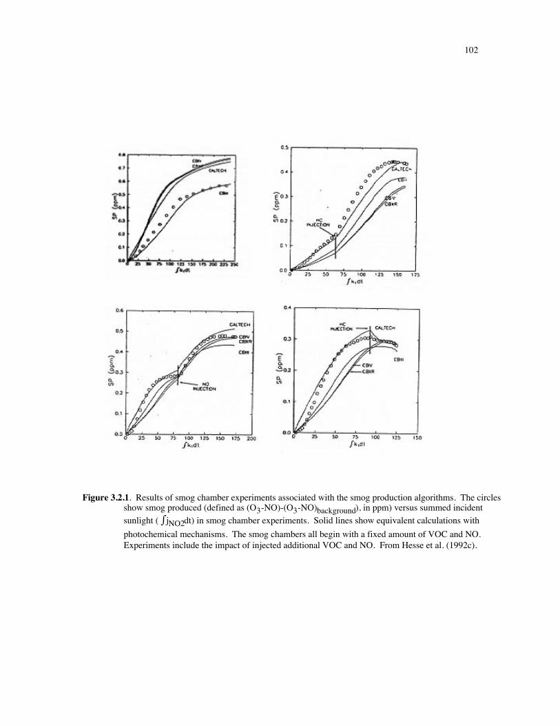
102

Figure 3.2.1. Results of smog chamber experiments associated with the smog production algorithms. The circlesshow smog produced (defined as (O3-NO)-(O3-NO)background), in ppm) versus summed incidentsunlight ( ∫ jNO2dt) in smog chamber experiments. Solid lines show equivalent calculations withphotochemical mechanisms. The smog chambers all begin with a fixed amount of VOC and NO.Experiments include the impact of injected additional VOC and NO. From Hesse et al. (1992c).

103

Figure 3.2.2. SPmax versus initial NOx concentration (in ppm) from UNC, SAPRC and CSIRO smog chamberexperiments. The regression line (solid line) is shown converted into concentration units. FromBlanchard et al. (1999).

104

3.2.4. Evaluations with 3-d models

Chang et al. (1997), Tonnesen and Dennis (2000b) and Blanchard and Stoeckenius (2001) all presented

evaluations of the smog production formulas against 3-d model predictions. These evaluations generally followed

the same format as used by Sillman (1995) for NOx-VOC indicators. Models were run for an initial scenario, an

equivalent scenario with reduced anthropogenic VOC throughout the model domain (typically by 25%-50%), and an

equivalent scenario with reduced anthropogenic NOx by the same percent. The predicted reduction in O3 at a

specific hour in the afternoon (corresponding to maximum or near-maximum O3) in the scenarios with reduced

VOC and reduced NOx was compared with the value of the extent parameter in the initial scenario at the same time

and location. The extent parameters were calculated from predicted species concentrations in the model scenario

and represent a potentially measurable quantity. The model evaluations generally used extent parameters based on

O3/NOy from Chang et al. (1997) (Equation 3.2.8) or Blanchard et al. (1999) (Equation 3.2.3). Blanchard et al.

(1999) also reported some results for the extent parameter based on NOx/NOy (Equation 3.2.5). Results for the

parameters based on NOx/NOy and O3/NOy are also discussed as contrary evidence in Section 3.2.5.

The general conclusion of the model-based studies is that an extent parameter below 0.6 is reliably associated

with VOC-sensitive conditions, and an extent parameter of 0.9 or above is reliably associated with NOx-sensitive

conditions. NOx-VOC sensitivity was variable for extent parameters between 0.6 and 0.9. The low (VOC-

sensitive) extent parameters are generally associated with urban centers in models. Extent parameters above 0.9

generally occurred in rural areas with relatively low O3 and little sensitivity to VOC or NOx. Blanchard and

Stoeckenius (2001) regarded extent parameters above 0.8 as representing NOx-sensitive conditions.

Chang et al. (1997) reported results for UAM-IV simulations (with CB-IV photochemistry) of events in

Baltimore and Los Angeles (Figure 3.2.3). Tonnesen and Dennis (2000b) reported results from RADM simulations

(with chemistry from Stockwell et al. 1990) of two events in New York (Figure 3.2.4). These results both used the

extent parameter from Chock et al. (1997).

Blanchard and Stoeckenius (2001) reported results from simulations using different versions of UAM or the

similar CAMx model for Los Angeles, Lake Michigan and southeast Texas, from simulations for the San Joaquin

valley using SAQM (Lu and Chang, 1998), and from simulations for Lake Michigan and the northeast corridor from

105

Sillman et al. (1993). These simulations all used versions of the CB-IV mechanism, except for the simulations from

Sillman et al. (1993) which used a modified form of Lurmann et al. 1986. Results are shown in Figure 3.2.5.

Blanchard and Stoeckenius did a similar analysis of the indicator ratios O3/NOy and O3/NOz. They concluded

the both the extent parameter and O3/NOy and O3/NOz could reliably separate NOx-sensitive and VOC-sensitive

locations, but only for relatively extreme values (extent below 0.6 or above 0.8, O3/NOy below 4 or above 8, and

O3/NOz below 5 or above 10). Blanchard and Stoeckenius also reported cases of erroneous or ambivalent results,

primarily for O3/NOy and O3/NOz but also for extent parameters, due to scenarios with different boundary

conditions (see Section 3.1.5). Tonnesen and Dennis, by contrast, reported that the other indicator ratios generated

a sharper separation of NOx-sensitive and VOC-sensitive locations in their model than the extent parameter.

106

(a) Baltimore

Figure 3.2.3. Predicted reduction in O3 resulting from a 25% reduction in anthropogenic VOC (X’s) and from a25% reduction in NOx (dashes), plotted against a version of the extent parameter (similar to Equation3.2.3) from simulations using UAM-IV for Baltimore and Los Angeles. From Chang et al. (1997).

107

(b) Los Angeles

Figure 3.2.3. Predicted reduction in O3 resulting from a 25% reduction in anthropogenic VOC (X’s) and from a25% reduction in NOx (dashes), plotted against a version of the extent parameter (similar to Equation3.2.3) from simulations using UAM-IV for Baltimore and Los Angeles. From Chang et al. (1997).

108

Figure 3.2.4. Predicted reduction in O3 resulting from a 30% change in anthropogenic VOC (+’s) (from +15% to–15% relative to base case emission rates) and from an equivalent 30% change in NOx (squares), plottedagainst the version of the extent parameter used by Chang et al. (1997) (similar to Equation 3.2.3) fromsimulations using RADM for New York City. From Tonnesen and Dennis (2000b).

109

Figure 3.2.5. Statistical summary of predicted response of peak ozone to a change in emissions of either NOx orVOC emissions versus extent of reaction parameter (Equation 3.2.3) in the model base case. Thestatistical summaries are presented as box plots, which show the 10th, 25th, 50th, 75th and 90th percentileresponse for all grid cells having O3 above 80 ppb and extent within 0.1-unit intervals (labeled using thelower limit of each interval). The dashed line shows the control response at the upwind model boundary.In contrast to the other figures in this report, positive responses represent an increase in O3 in response toreduced emissions. Negative responses represent a reduction in O3 in response to reduced emissions.From Blanchard and Stoeckenius (2001).

110

3.2.5. Contrary evidence

Sillman and He (2002) reported results from the five simulations shown in Table 3.1.1. These results included

all three versions of the extent parameter proposed by Blanchard et al. (1999). They found a correctible flaw in the

extent parameter based on O3/NOy and fundamental problems in the extent parameters based on NOx/NOx and

O3/NOx. Results are shown in Figures 3.2.6 and 3.2.7.

As shown in Figure 3.2.6, NOx- sensitive locations are generally associated with high values of the first extent

parameter (above 0.9) and VOC-sensitive locations are associated with low values (below 0.6). However there is

also considerable overlap between NOx-sensitive and VOC-sensitive parameter values. Strongly VOC-sensitive

locations have extent parameters as high as 0.9, and strongly NOx-sensitive locations include extent parameters as

low as 0.6. This result is not dissimilar to the model-based results reported in Figures 3.2.3, 3.2.4 and 3.2.5 but is

given a different emphasis. There is significantly less overlap between NOx-sensitive and VOC-sensitive locations if

the ratio (O3-O3b)/(NOy-NOyb) were used instead of the extent parameter (see Figure 3.1.2). This ratio, discussed

as a NOx-VOC indicator in Section 3.1.3b, is actually very similar to the original extent parameter (equation 3.2.2)

proposed by Johnson.

Figure 3.2.7 shows the same results in the form of extent parameters plotted versus O3. The locations in this plot

have been classified as NOx-sensitive, mixed or VOC-sensitive as was done above in Figure 3.1.7, using definitions

described in Section 3.1.10. Here, it appears that the extent parameter can consistently separate NOx-sensitive and

VOC-sensitive locations, but that the transition between NOx-sensitive and VOC-sensitive locations changes

between regions of low and high ozone. Locations with O3 between 80 and 120 ppb fit the description given by

Blanchard and Stoeckenius, with VOC-sensitive conditions corresponding to extent below 0.6 and NOx-sensitive

conditions corresponding to extent above 0.8. For O3 above 130 ppb, locations with extent equal to 0.8 or below

are almost all VOC-sensitive, locations with extent above 0.95 (including many locations with extent greater than 1)

are NOx-sensitive. By contrast, the ratio (O3-O3b)/(NOy-NOyb) shows a consistent pattern for both low and high

O3, with VOC-sensitive conditions corresponding to (O3-O3b)/(NOy-NOyb) below 4 and NOx-sensitive conditions

corresponding to (O3-O3b)/(NOy-NOyb) above 6.

111

This comparison suggests that the modified form proposed by Chang et al. and Blanchard et al. (involving

O3/NOya rather than O3/NOy) may be a mistake for ambient conditions. Isopleth plots for (O3-O3b)/(NOz-NOzb)

based on a 0-d model and constant emissions (Figure 3.1.3, Section 3.1.4) are also consistent with this result.

Results obtained with the extent parameters based on NOx/NOy and O3/NOx, also shown in Figures 3.2.6 and

3.2.7, show a much weaker correlation with NOx-VOC sensitivity. For the extent parameter based on NOx/NOy,

parameter values below 0.6 are consistently associated with NOx disbenefits. Locations with the highest values also

include the strongest predicted NOx benefits. However, parameter values above 0.7 include both NOx-sensitive and

VOC-sensitive locations, and strongly VOC-sensitive locations can be found with extent parameters as high as 0.98.

The poor results are associated largely with the model for Lake Michigan reported by Sillman et al. (1993). In this

model a strongly VOC-sensitive plume from the Chicago area is transported across Lake Michigan and remains

VOC-sensitive even after most of its NOx has reacted away. However, the other models also include strongly

VOC-sensitive locations with extent close to 0.9. The extent parameter based on O3/NOx also shows ambiguous

results. As in the case of NOx/NOy, contrary results occur because ozone can retain VOC-sensitive characteristics

even after most of its NOx has reacted away.

Calculations with the 0-d model described in Section 3.1.4 also provide contrary evidence concerning the extent

parameter based on NOx/NOy. As shown in isopleth plots (Figure 3.2.8), a high value of NOx/NOy

(corresponding to a low extent parameter) is associated with strongly NOx-saturated conditions. However, low

values of NOx/NOy are associated with either NOx-sensitive or VOC-sensitive conditions. The isopleth pattern for

(O3-O3b)/NOz, shown above in Figure 3.1.4, correlates more closely with NOx-VOC sensitivity. These isopleth

plots are based on calculations with continuous emissions. By contrast, the smog chamber experiments used to

derive the extent parameters were all based on an initial high concentration of NOx and VOC.

112

-80-60-40-20

020406080

0 0.5 1 1.5

Extent of reaction 1 .

Ozo

ne r

educ

tion

(ppb

)


-80-60-40-20

020406080

0 0.2 0.4 0.6 0.8 1


Ozo

ne r

educ

tion

(ppb

)


-80-60-40-20

020406080

0.4 0.6 0.8 1


Ozo

ne r

educ

tion

(ppb

)


Figure 3.2.6. Predicted reductions in ozone in response to a percent reduction in emissions of anthropogenic VOC(crosses), and predicted reductions in response to the same percent reduction in emissions ofanthropogenic NOx (green circles), plotted versus model values for three extent parameters (B1, B2 andB3, defined in Equations 3.2.3, 3.2.5 and 3.2.8), for the five model scenarios from Table 3.1.1. Percentreductions are either 25% or 35% in individual scenarios. Based on results shown in Sillman and He(2002).

0

0.2

0.4

0.6

0.8

1

1.2

1.4

1.6

0 50 100 150 200 250

O3 (ppb) .

Exte

nt o

f re

actio

n 1

NOx-sensitive

Mixed

VOC-sensitive

NOx titration

(O3-O3b)/NOy^.67

(a) ExtentB1 (Equation 3.2.3).

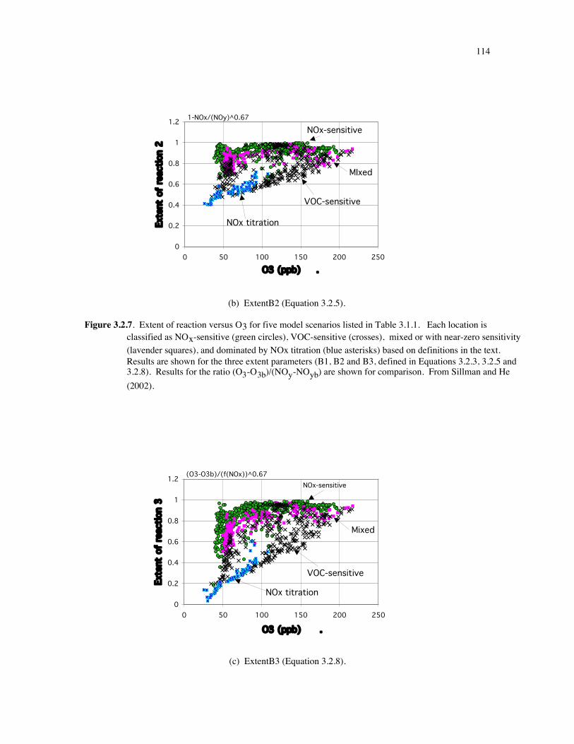
114

0

0.2

0.4

0.6

0.8

1

1.2

0 50 100 150 200 250

O3 (ppb) .

Exte

nt o

f re

actio

n 2

1-NOx/(NOy)^0.67

NOx-sensitive

MIxed

VOC-sensitive

NOx titration

(b) ExtentB2 (Equation 3.2.5).

Figure 3.2.7. Extent of reaction versus O3 for five model scenarios listed in Table 3.1.1. Each location isclassified as NOx-sensitive (green circles), VOC-sensitive (crosses), mixed or with near-zero sensitivity(lavender squares), and dominated by NOx titration (blue asterisks) based on definitions in the text.Results are shown for the three extent parameters (B1, B2 and B3, defined in Equations 3.2.3, 3.2.5 and3.2.8). Results for the ratio (O3-O3b)/(NOy-NOyb) are shown for comparison. From Sillman and He(2002).

0

0.2

0.4

0.6

0.8

1

1.2

0 50 100 150 200 250

O3 (ppb) .

Exte

nt o

f re

actio

n 3

(O3-O3b)/(f(NOx))^0.67NOx-sensitive

Mixed

VOC-sensitive

NOx titration

(c) ExtentB3 (Equation 3.2.8).

115

0

2

4

6

8

10

12

0 50 100 150 200 250

O3 (ppb) .

dO3/

dNO

y

NOx-sensitive

Mixed

VOC-sensitive

NOx titr.

(d) (O3-O3b)/(NOy-NOyb)

Figure 3.2.7. Extent of reaction versus O3 for five model scenarios listed in Table 3.1.1. Each location isclassified as NOx-sensitive (green circles), VOC-sensitive (crosses), mixed or with near-zero sensitivity(lavender squares), and dominated by NOx titration (blue asterisks) based on definitions in the text.Results are shown for the three extent parameters (B1, B2 and B3, defined in Equations 3.2.3, 3.2.5 and3.2.8). Results for the ratio (O3-O3b)/(NOy-NOyb) are shown for comparison. From Sillman and He(2002).

116

Figure 3.2.8. Isopleths for NOx/NOy as a function of the average emission rate for NOx and VOC (1012 molec.cm-2 s-1) in 0-d calculations. The isopleths represent conditionsduring the afternoon following 3-daycalculations, at the hour corresponding to maximum O3. Isopleths are shown as solid green lines.Isopleths for O3 in ppb (red dashed lines) are superimposed (see also Figure 1.2 and Figure 3.1.4). Theshort blue dashed line represents the transition from VOC-sensitive to NOx-sensitive conditions. FromSillman and He (2002).

117

3.2.6. Uncertainties associated with the theoretical basis

One problem with the extent parameters is the lack of a theoretical justification that would provide a causal link

between extent parameters and NOx-VOC sensitivity.

It is generally known that locations near urban centers and other large emission sources are often VOC-sensitive,

while downwind locations are often NOx-sensitive (Milford et al., 1989; 1994). It is also known that plumes from

urban areas and power plants tend to change from NOx-saturated to NOx-sensitive as they move downwind (Milford

et al., 1994; Gillani et al., 1996). This trend has been attributed to the more rapid removal of NOx relative to VOC

as a plume moves downwind, causing its VOC/NOx ratio to increase. The trend is also due to the presence of

biogenic VOC in rural areas. However, there is no reason why the transition from VOC-sensitive to NOx-sensitive

conditions should be associated with a certain extent of reaction.

Ozone isopleth plots generally show that air with a high ratio of VOC to NOx should have NOx-sensitive

chemistry, regardless of whether the air consists of fresh or aged emissions. In theory, NOx-sensitive chemistry is

possible even with an extent parameter near zero, if emissions consist of strongly reactive VOC and a high

VOC/NOx ratio. No such conditions have appeared in either the smog chamber experiments or in the model results,

but these may be based more on the specific conditions in the tests.

The extent parameters are all based on the assumption that cumulative ozone production per NOx reaches a

specified value in aged air, after most of the emitted NOx has reacted away, and that the final ozone production per

NOx is unaffected by the amount of VOC. Ryerson et al. (2001) reported that ozone production per NOx varies by a

factor of 3 among plumes from power plants and with urban areas, even after the plume NOx content has largely

reacted away. Figure 3.2.9 compares measured O3 versus NOz in two power plant plumes, both with similar

reactive nitrogen content but with different amounts of biogenic VOC. Extent of reaction was similar in both

plumes (NOx/NOy=0.2, and ExtentB2 parameter from equation 3.2.5 equal to 0.86), but ozone produced and ozone

production per NOx (shown as ozone per NOz) was much higher in the plume with high biogenic VOC. The

different ozone content in these two plumes contradicts the theoretical basis of the extent of reaction parameters.

In this context, the smog production algorithms based on the ratio O3/NOy can be viewed as representing both

extent of reaction (1-NOx/NOy) and the rate of ozone production per NOx (O3/NOz). As described in Section

3.1.12, the rate of ozone production per NOx (also known as ozone production efficiency) is associated with NOx-

118

sensitive versus VOC-sensitive chemistry. The smog algorithm based on NOx/NOy is only associated with extent

of reaction, and not with the rate of ozone production per NOx. This may explain its poor performance in models.

Figure 3.2.9. Measured O3 versus NOz in aircraft transects downwind of two power plant plumes: Thomas Hill(dots) and Johnsonville (circles). These power plants have similar rates of NOx emissions, and 80% ofthe original NOx had been oxidized in each transect. Johnsonville, with higher input from biogenicVOC, had higher O3. From Ryerson et al. (2001).

119

3.2.7. Applications of the smog production algorithms

The smog production algorithms have been used widely to interpret measurements in many urban areas in the

U.S. Blanchard (2001) described applications in six regions in the U.S.: the northeast corridor, southern Lake

Michigan, Atlanta, Texas (including Houston and Dallas), central California and southern California. These

applications often included measurements for extended time periods, including several years, and provide a broad

characterization of inferred NOx-VOC sensitivity in urban areas. Blanchard et al. (1999) described applications to

southern California and Lake Michigan in greater detail. Chang and Suzio (1996) also describe applications of the

method during episodes in New York and the surrounding region, Washington D.C., Atlanta and Houston.

Applications of the method have also been made in Melbourne, Australia and Auckland, New Zealand.

Figures 3.2.10 and 3.2.11 show results of the applications to southern Lake Michigan and Los Angeles. As

shown here, the method characteristically shows VOC-sensitive conditions in urban centers and mixed or NOx-

sensitive conditions in rural areas.

In the broad application by Blanchard (2001), approximately half of the measured values represented VOC-

sensitive conditions (extent below 0.6) and half represented mixed conditions (extent between 0.6 and 0.9). Values

corresponding to NOx-sensitive conditions (extent above 0.9) were measured approximately 10% of the time and

these measurements generally occurred in rural locations. These results are summarized in Table 3.2.1.

In general, applications of the method have consisted primarily of calculating the values of the smog production

parameter and presenting the interpretation in terms of NOx-VOC sensitivity. Comparatively little analysis of

ambient measurements has been done that might evaluate the accuracy of the measurements or whether the method

is applicable to local conditions. No comparisons have been made between ambient measurements of smog

production parameters and results of 3-d photochemical models.

Evaluations of the viability of the method based on ambient measurements and results from models that might be

used to evaluate measurements are described in the next section (Section 3.2.8).

120

Figure 3.2.10. Application of smog chamber algorithms to southern California. The size of the circles areproportional to peak O3 at each site. White shadings in each circle represent percent of the time (over aperiod from 7am to 6pm) with extent below 0.6; gray shadings represent extent between 0.6 and 0.9,and black shadings represent extent greater than 0.9. From Blanchard et al., 1999.

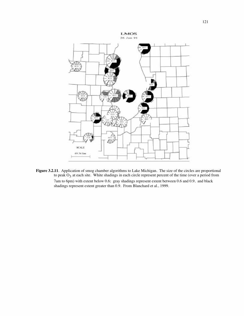
121

Figure 3.2.11. Application of smog chamber algorithms to Lake Michigan. The size of the circles are proportionalto peak O3 at each site. White shadings in each circle represent percent of the time (over a period from7am to 6pm) with extent below 0.6; gray shadings represent extent between 0.6 and 0.9, and blackshadings represent extent greater than 0.9. From Blanchard et al., 1999.

122

Table 3.2.1

Measured exent of reaction parameters

Summary of measured extent-of-reaction parameters at locations in the U.S. over a ten-year

period. Extent was calculated from measured O3 and NOx from EPA monitors. The table shows

the frequency of occurence of extent values below 0.6 (“VOC-sensitive”), between 0.6 and 0.9

(“transitional”), and above 0.9 (“NOx-sensitive”) for all monitors during hours when ozone

concentrations were greater than 80 ppbv, along with the total number of at each site.

Extent of Reaction (percent of hours)Domain Years Total

HoursVOC-limited

Extent < 0.6

Transitional

0.6#Extent<0.9

NOx-limited

Extent $ 0.9

Central California

San Francisco

Bay Area

1991-98 4269 81.3 18.1 0.6

Sacramento Valley1994-97 4133 38.4 43.6 18.0

San Joaquin Valley1994-97 36293 32.4 60.2 7.5

Southern California

South Central Coast1994-97 11826 42.8 47.8 9.4

South Coast 1994-97 65416 74.4 24.6 1.0

Mojave 1994-97 15991 32.9 56.0 11.1

Salton Sea 1994-97 2844 32.6 54.6 12.8

San Diego 1994-97 6655 80.6 18.9 0.4

123

Texas

Houston1994-99* 2979 41.9 43.5 14.6

Beaumont-Port Arthur1994-99* 509 21.6 56.4 22.0

Dallas-Fort Worth 1994-99* 1777 39.6 48.0 12.4

El Paso 1994-99* 337 74.2 21.1 4.7

Lake Michigan

1991 492 13.8 40.7 45.5

1994-98 2271 38.9 42.3 18.8

Northeast and Mid-Atlantic

Connecticut1994-99 1482 50.1 40.1 9.7

Washington, DC 1994-99 1692 51.7 38.4 10.0

Delaware 1995-99 416 53.8 40.9 5.3

Maine 1995-99 368 8.7 52.2 39.1

Maryland1994-99 610 37.5 53.3 9.2

Massachusetts 1995-99 1783 30.0 56.1 13.9

New Jersey 1995-99 1551 16.7 56.8 26.5

New York1995-99 1071 72.5 26.3 1.0

124

North Carolina 1995-99 3567 39.4 56.0 4.6

Pennsylvania 1995-99 1381 51.4 42.9 5.6

Rhode Island 1995-99 162 25.3 45.1 29.6

Virginia 1994-99 513 52.2 31.0 16.8

Atlanta

1 upwind,

3 central,

2 downwind sites

1990 736 54.1 39.7 6.3

3 downwind sites 1994-99 3148 13.3 48.7 38.0

* 1999 is a partial year

125

3.2.8. Evaluations with ambient measurements.

Blanchard and Stoeckenius (2001) reported correlation plots from a series of 3-d models, comparing model

values of SP and SPmax (derived from species concentrations in the model) as a function of model NOy. Typically,

these plots showed a broad range of the SP parameter. The parameter SPmax is closely correlated with NOx and

represents an effective maximum value for the range of SP. These correlations, shown in Figure 3.2.12, may also

provide a basis for evaluating an ambient data set. The correlation plot of SP versus NOy shows the same type of

scatter predicted for O3 versus NOy (see Figure 3.1.7), which also might provide a basis for evaluating ambient data.

Blanchard (2001) also analyzed ambient measurements from five cities in order to identify the impact of

uncertainty associated with measurements. The smog parameters were derived from measured O3 and NOx, where

NOx was measured using commercial chemilluminescent instruments. These measurements generally represent the

sum of true NOx plus uncertain percentages of organic nitrates and HNO3. Blanchard derived smog production

parameters from this data in two ways, by interpreting the measurements as NOx and applying Equation 3.2.6 or by

interpreting the measurements as NOy and applying equation 3.2.3. A comparison between the two alternative

parameters (Figure 3.2.13) showed relatively little difference for values below 0.6 (corresponding to VOC-sensitive

conditions). Large differences occurred for values above 0.6, which included the majority of the data set. When

measurements are interpreted as NOx, the extent values are almost all below 0.9. If interpreted as NOy, extent

values would be as high as 2.

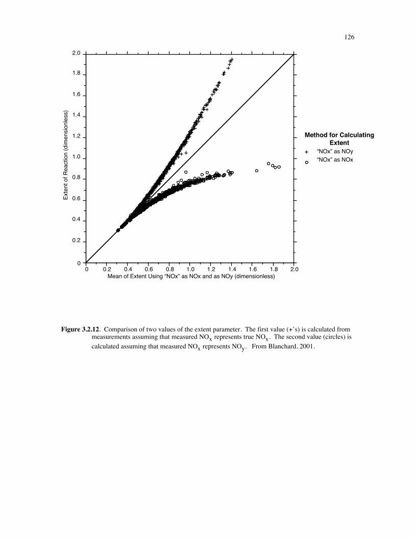
126

Figure 3.2.12. Comparison of two values of the extent parameter. The first value (+’s) is calculated frommeasurements assuming that measured NOx represents true NOx. The second value (circles) iscalculated assuming that measured NOx represents NOy. From Blanchard, 2001.

0

0.2

0.4

0.6

0.8

1.0

1.2

1.4

1.6

1.8

2.0

Exte

nt o

f Rea

ctio

n (d

imen

sionl

ess)

0 0.2 0.4 0.6 0.8 1.0 1.2 1.4 1.6 1.8 2.0Mean of Extent Using “NOx” as NOx and as NOy (dimensionless)

“NOx” as NOx“NOx” as NOy

Method for CalculatingExtent

127

3.3 CONSTRAINED STEADY STATE AND OTHER ANALYSES BASED ON AMBIENT VOC AND NOx


• Constrained steady state (CSS) refers to a series of calculations, based on ambient VOC and NOx, that seeks to

identify how the instantaneous rate of ozone production varies in response to changed NOx and VOC. In

addition to these calculations, simple formulas have been developed to determine the sensitivity of

instantaneous ozone production to NOx and VOC based on measured NOx and VOC.

• Because measured NOx and VOC are closely related to emission inventories, methods that would use

measurements to evaluate inventories are also included here.

• Two similar forms of constrained steady state calculations have been used: the Observation-based Model by

Cardelino and Chameides (1995, 2000) and the constrained steady state model developed by Kleinman et al.

(1997, 2000). These both consist of 0-d calculations driven by ambient NOx and VOC measurements.

• Tonnesen and Dennis (2000a) and Kirchner et al. (2001) both derived simple formulas that relate NOx-VOC

sensitivity of instantaneous ozone production to the ratio of reactivity-weighted VOC to NOx. Kleinman et al.

(1997, 2000) developed a somewhat more complicated formula in terms of VOC, NOx, and sources of odd

hydrogen radicals.

• No reliable way has been developed to determine the NOx-VOC sensitivity of ozone concentrations based on

measured NOx and VOC. However, average O3-NOx-VOC sensitivity in Eulerian AQMs is broadly similar to

the sum of calculated instantaneous NOx-VOC sensitivity rates.

• Accuracy of VOC measurements is a major concern for CSS and all other methods that rely on measured VOC.

Measurements of highly reactive VOC are especially uncertain.

• CSS calculations must be based on measurements that include all directly emitted VOC. If some directly

emitted species are omitted from the measurements, their concentrations must be estimated based on estimated

ratios relative to measured species. Complete omission of unmeasured species would bias the CSS calculation.

• Additional uncertainties of these methods include the likely variation of short-lived VOC with altitude and the

possibility that individual measurements are affected by on-site emissions. Methods such as CSS effectively

assume that surface measurements are representative of the entire convective mixed layer, in which ozone is

formed.

128

• CSS calculations by themselves do not include methods for identifying errors or uncertainties. These sources of

error can often be identified if the CSS calculation is combined with a more direct analysis of measurements,

focusing on measured correlations among VOC.

• Because measured VOC and NOx are closely related to emission inventories, it may be useful to use these

measurements as a basis for evaluating and modifying emission inventories in addition to (or instead of)

calculating NOx-VOC sensitivity directly. Methods for evaluating emission inventories from measurements

include (i) analysis of species correlations and (ii) inverse modeling using standard 3-d air quality models.


• Three alternative approaches involving ambient NOx and VOC are feasible for use in evaluating ozone

chemistry: (i) a full CSS calculation from ambient data; (ii) a simple rule-of-thumb for instantaneous NOx-

VOC sensitivity, such as the ratio of reactivity-weighted VOC to NOx, and (iii) evaluation and modification of

emission inventories based on ambient measurements.

• A full CSS calculation (such as the model developed by Cardelino and Chameides) could easily be developed

and made available to regulators. CSS calculations are much easier to use than Eulerian AQMs, and evaluation

of measured VOC and NOx with a CSS calculation would be no more difficult than a direct analysis of the data

without the CSS calculation.

• In contrast with other methods, it is likely that a reliable, simple rule can be developed that identifies

instantaneous NOx-VOC chemistry in terms of reactivity-weighted NOx and VOC. It is also fairly certain that

ambient VOC and NOx are directly related to O3-NOx-VOC sensitivity.

• CSS calculations and associated rules for interpreting measured VOC and NOx are potentially useful for

analyzing seasonal trends in apparent O3-NOx-VOC sensitivity and to identify differences between individual

events and locations.

• No formal method has been developed for using CSS approaches in combination with standard 3-d air quality

modeling. CSS model results might be used to confirm or deny the general conclusions of an air quality model.

Formal methods of comparison between CSS calculations and AQMs might be developed. However it may be

more useful to use measured VOC and NOx as a basis for evaluating and modifying emission inventories in

AQMs.

129

• Analyses based on measured NOx and VOC should include comparisons that would evaluate measurement

accuracy. CSS calculations are unreliable unless a complete set of measurements of primary VOC is available,

including accurate measurement of highly reactive VOC.

3.3.3. Constrained steady state models

Constrained steady state models consist of 0-d calculations of photochemical processes, often with little or no

time component. These calculations are widely used to investigate the concentrations of short-lived radical species

such as OH and HO2 (e.g. McKeen et al., 1997; Tan et al., 2001). In a constrained steady-state calculation the

long-lived species are all derived from measured concentrations or from assumptions about ambient conditions. The

short-lived species are then calculated with the assumption that they are in steady state. In addition, calculations of

this type often use measured photolytic rate constants if these measurements are available. Dynamics, including

possible dilution through vertical mixing and horizontal advection, are not included.

The CSS calculations are generally not useful unless measurements include a relatively complete set of directly

emitted VOC. Intermediate organics might be estimated as part of the calculation (see next paragraph). Directly

emitted species must be set as part of the initial conditions of the calculation.

CSS calculations must make assumptions about the concentrations of unmeasured organics, usually including

aldehydes and other reaction products of directly emitted hydrocarbons, and potentially short-lived organic nitrates

such as PAN. In the CSS model used by Kleinman et al. (1997, 2000, 2001), PAN and relatively short-lived

intermediate organics (e.g. methylvinyl ketone) were generally assumed to be at steady state.

The observation-based model developed by Cardelino and Chameides consisted of a similar 0-d calculations with

a more sophisticated method for establishing concentrations of intermediate VOC. Their model consisted of 0-d

calculations that were performed for full day rather than for a fixed point in time as done by Kleinman et al. The

calculations represented a convective mixed layer that increased with height (entraining air from aloft) as the day

progressed. Pseudo-emission terms were added to insure that all measured species were constrained to remain at

measured values. Unmeasured species (aldehydes, PAN) were allowed to accumulate throughout the time period of

the calculation based on photochemical production and removal. A dilution factor was also applied to the

unmeasured species to represent the growth of the convective mixed layer. No dilution due to horizontal transport

was included.

130

Cardelino and Chameides also modified the CB-IV chemistry in their calculation so that directly emitted VOC

and secondary reaction products were not lumped into a single species. Species categories in the CB-IV mechanism

that included both primary and secondary species (e.g. ALD2, which is used to represent both secondary aldehydes

and directly emitted alkenes) were separated into two species.

Kleinman et al. and Cardelino and Chameides both calculated the production rate of ozone and used the

calculated production rate to make predictions about NOx-VOC sensitivity. In both cases the calculation was

repeated with reduced NOx and reduced VOC. Changes in ozone production rates were recorded in a form adopted

from the Relative Incremental Reactivity (RIR) format (Carter, 1995):

RIR =DPO3 PO3

DS S (3.3.1)

where DPO3 represents the difference between the ozone production rate (PO3) in the initial calculation and the

ozone production rate in a calculation with concentrations of a precursor S (either NOx or VOC) changed by an

amount DS. Kleinman calculated ozone production and precursor sensitivity at individual time periods. Cardelino

and Chameides summed the calculated production and precursor sensitivity over a 12-hour time period. The sum

used by Cardelino and Chameides effectively gives greater weight to NOx-VOC sensitivity at times and places with

higher rates of ozone production.

The CSS calculations do not generate any model predictions that can be evaluated in comparison with

measurements. In effect, measurements only provide input to the calculations. Summed ozone production in the

calculations cannot be directly compared to measured O3. However, Kleinman’s results also established a relation

between instantaneous NOx-VOC chemistry and concentrations of odd hydrogen radicals, which might be evaluated

against ambient measurements (see Section 3.3.4).

3.3.4. Short formulas for NOx-VOC sensitivity.

Tonnesen and Dennis (2000a) and Kirchner et al. (2001) independently derived a simplified formulas for

determining the sensitivity of ozone production rates to precursor emissions. Tonnesen and Dennis used a 3-d

simulation for the northeastern U.S. (using RADM) as the basis for evaluating instantaneous ozone production.

They used simulations with changed NOx and VOC emissions to identify the change in the ozone production rate

131

associated with changed emissions. These changes were then correlated with possible indices for the sensitivity of

ozone production rates (see Figure 3.3.1).

Tonnesen and Dennis derived several formulas that correlate with the NOx-VOC sensitivity of instantaneous

production, including the ratio of rates of production of H2O2 and HNO3. The ratios most likely to be useful for

regulatory purposes were: (i) O3/NOx; and (ii) a ratio based on rVOC/NOx. The exact ratio used by Tonnesen and

Dennis was:

I(HC, NO2) =g km[HC]mÂ

g km[HC]m + ka[NO2 ]Â (3.3.2)

where g (=1.3) represents an adjustment factor to account for unmeasured VOC. A simple ratio of reactivity-

weighted VOC to NO2 is related to their formula by

rVOCrNO2

=I(HC,NO2 )

1- I(HC, NO2 ) (3.3.3)

Tonnesen and Dennis found that VOC-sensitive instantaneous chemistry corresponds to I(HC,NO2) less than 0.8

and NOx-sensitive chemistry corresponds to I(HC,NO2) greater than 0.85. These are equivalent to rVOC/rNO2 less

than 4 and greater than 5.7. Kirchner et al. (2001) gave approximately the same values, expressed as rNO2/rVOC,

using the RACM mechanism (Stockwell et al., 1997).

These results have not been tested elsewhere, but some form of this formula might provide a convenient basis for

interpreting measured VOC and NOx. Use of the ratio rVOC/NOx might also be compared with formulas based on

analysis of ozone formation potential (e.g. Carter et al., 1994, 1995).

Kleinman et al. (1997, 2000, 2001) devised a more complicated formula. Kleinman et al. found that the NOx-

VOC sensitivity of instantaneous ozone production was consistently correlated with the parameter LN/Q, which

related the loss rate for NOx (LN) to the rate of production of primary odd hydrogen radicals (Q). They found that

NOx-sensitive chemistry was always associated with LN/Q below 0.5 and that VOC-sensitive chemistry was always

associated with LN/Q above 0.5. The same relation between instantaneous NOx-VOC sensitivity and LN/Q was

found in constrained steady state calculations based on measurements in Nashville, New York and Phoenix.

Kleinman et al. also found that the division between instantaneous NOx benefits versus disbenefits occurred when

132

LN/Q was equal to 0.67. These results were similar to the photochemical analysis associated with NOx-VOC

indicators (Section 3.10). Kleinman et al. developed a formula for the NOx-VOC sensitivity of instantaneous ozone

production, as a function of LN/Q. More recently, Kleinman et al. (2001) proposed that the same LN/Q could be

calculated directly from measurements of ambient NO, NO2, VOC, and the parameter Q. They proposed that Q

could be determined from measured O3, HCHO and photolytic rate constants.

The Kleinman formula was calculated based on a single photochemical mechanism (RADM), but there is a good

chance that the formula will be universal. Unlike the simpler rVOC/NOx ratio, the LN/Q formula accounts for

variations with sunlight and has been used in model calculations at different times of day. The correlation between

calculated NOx-VOC sensitivity and LN/Q is also much stronger than between rVOC/NOx (see Figure 3.3.2). The

major limitation of the LN/Q formula is that it requires measurements that may not be available. The parameter Q

requires measured HCHO. In addition, locations with high alkenes (e.g. Houston) may have Q influenced by other

organics. Kleinman’s correlation is especially useful for research, because directly measured OH and HO2 might be

used directly to evaluate the LN/Q formula (Thornton et al., 2002).

In terms of rVOC and NOx, Kleinman’s formula can be approximated as: rVOC2Q

NOx4 . This contrasts with the

simpler ratio rVOC/NOx, which was used by Tonnesen and Dennis (2000a), Kirchner et al. (2001) and Chameides

et al. (1992).

The exact formula proposed by Kleinman is as follows:

LNQ

= 0.5 -a + a 2 + 4a( ) (3.3.3a)

a =k1[NO2 ]k3g [NO]

k2[VOC]

Ê

Ë Á Á

ˆ

¯ ˜ ˜

2 12Qkeff

Ê

Ë Á Á

ˆ

¯ ˜ ˜ (3.3.3b)

where k1 represents the reaction rate of OH with NO2, k2 represents the reaction rate of individual VOC with

OH (summed over all VOC), k3 represents the reaction rate of HO2 with NO, g is the ratio of HO2 to HO2+RO2,

and keff is the combined rate constant for HO2+HO2 and HO2+RO2.

133

Figure 3.3.1. Predicted change in the rate of ozone production in response to a percent change in VOC (+’s) or inNOx (squares), plotted versus an index that is a function of reactivity-weighted VOC and NO2(I(HC,NO2, Equation 3.3.2). The change in ozone production is represented as percent relative topercent change in NOx or VOC. Results are for RADM simulations of New York (Tonnesen et al.,2000a).

Figure 3.3.2. Predicted sensitivity of the instantaneous ozone production rate to changes in NO and VOC, based oncalculations with the constrained steady state (CSS) model driven by measurements from the 1998 DOEfield campaign in Phoenix. Sensitivity is reported as the percent change in ozone production relative tothe percent change in NO or VOC (dlnP(O3)/dln[NO] and dlnP(O3)/dln[VOC]) and is shown as afunctionof the ratio of photochemical removal of NOx to the radical source (LN/Q, defined in Section 3.3.4). Thesquares show results of the CSS calculation. The lines show results of the analytic formula (Equation3.3.3).

134

3.3.5. Integrating from instantaneous ozone production to ozone concentrations

A major limitation of the CSS calculations is that they only give NOx-VOC sensitivity associated with the

instantaneous rate of ozone production. They do not provide direct information about how ozone concentrations

depend on NOx and VOC. The NOx-VOC dependence of ozone concentrations depends on photochemical

production over time periods of several hours, and sometimes over several days, and involves transport from distant

locations. The NOx-VOC dependence of ozone at an individual site is often very different from that which would

be predicted from the instantaneous photochemistry at the site.

Cardelino and Chameides (1995) compared results of their CSS model with results of an Eulerian AQM for a

single episode in Atlanta. They used VOC and NOx concentrations from the AQM as pseudo-observations to drive

the CSS calculation, thus producing an equivalent CSS calculation for an AQM that was in perfect agreement with

ambient measurements. They examined NOx-VOC sensitivity predictions from the AQM for (i) peak O3, (ii)

locations with O3 greater than 120 ppb; and (iii) locations with O3 greater than 100 ppb. This was compared with

the NOx-VOC sensitivity found for the 12-hour summation of instantaneous PO3 from the CSS calculations. They

found that NOx-VOC sensitivity for peak O3 in the AQM was comparable to the 12-hour summation based on

pseudo-observations at a single downtown location, and that NOx-VOC sensitivity for O3 above 100 ppb and above

120 ppb in the AQM was comparable to the 12-hour summation based on the downtown location and four suburban

locations within 20 km of downtown. These results suggest a broad correlation between CSS calculations and O3-

NOx-VOC sensitivity, but they do not prove that the same relation would hold in all locations or during events with

different meteorology.

In a case study of the New York metropolitan area, Kleinman et al. (2000) found that CSS calculations in the

entire metropolitan area were consistent with VOC-sensitive chemistry. Because the calculations included

measurements that extended from near downtown out to the downwind region with the highest O3, they concluded

that the evidence was consistent with VOC-sensitive ozone concentrations. This conclusion was also consistent

with observed O3 and NOy, interpreted as an indicator ratio.

Kirchner et al. (2001) investigated the use of reactivity-weighted VOC/NOx as evidence for O3-NOx-VOC

sensitivity in Eulerian AQM simulations for Athens and the Swiss plateau. They introduced tracers in their model

representing low (VOC-sensitive) rVOC/NOx and high (NOx-sensitive) rVOC/NOx at 8 am, and compared the

135

distribution of these tracers with the impact of reduced VOC and NOx in their model. The VOC and NOx

reductions were applied just for a one-hour period (8-9 am) to avoid complications that would be caused by varying

chemistry along the transport path. They found that predicted sensitivity to the reduced NOx and VOC was strongly

correlated with the amount of NOx-sensitive and VOC-sensitive tracer at each model location. The correlation

between NOx-VOC sensitivity and the tracers was stronger than the correlation with the indicator ratio O3/NOz and

comparable to the correlation with the ratio H2O2/HNO3. It is unclear whether the same results would be found for

emission reductions applied throughout the day.

The evidence suggests that CSS calculations and rVOC/NOx are likely to be correlated with O3-NOx-VOC

sensitivity in general, but it is not certain whether this correlation is universal. The possibility of varying results for

different locations and for different events are comparable to the possibility of varying results associated with

indicator ratios.

3.3.6. Accuracy and completeness of NOx and VOC measurements

Questions of accuracy have been raised about measurements of both VOC and NOx, especially associated with

the PAMs network.

In order to provide meaningful results, CSS calculations and other related methods require measurements that

include all directly emitted VOC. Secondary VOC can be incorporated into the calculation as described in Section

3.3.3. If unmeasured primary species are omitted, then the resulting calculation will have VOC reactivity that is

lower than probable ambient conditions and will constantly give biased NOx-VOC predictions. Biogenic VOC are

especially important in this context. Highly reactive anthropogenic VOC are also important. The issue of reactive

VOC was highlighted by the recent Texas Air Quality Study, in which it appeared that fast-reacting alkenes had a

major impact on ozone formation.

Unmeasured anthropogenic VOC can be estimated by using ratios between individual VOC species that were

established from previous data sets. Parrish et al. (2000) reported that correlations among individual VOC often

suggest that these species are present in similar ratios throughout the U.S. This is especially true among closely

related species (e.g. individual alkenes or individual aromatics). Parrish et al. (2000, 1998) report observed ratios

for many of these species.

136

Parrish et al. found that individual measurements of alkenes, especially in the PAMS network, are subject to

considerable uncertainty. They found that the distribution of species in PAMS measurements frequently showed a

pattern that was comparable to that of fresh auto emissions, without any sign of photochemical aging. This might be

due to the impact of on-site emissions at many PAMS sites, or it might be due to general uncertainties associated

with measured alkenes. Parrish et al. (1998) reported an intercomparison among 33 measured ensembles of

speciated VOC, and found that mean values were within 4% of a reference measurement. However, the individual

measured average VOC concentrations had biases ranging from 45% low to 85% high. Comparisons among

individual measurements of alkenes, aromatics and isoprene showed scatter of +/-38%, +/-47% and +/-80%

respectively. In addition, Parrish et al. (1998) reported evidence of systematic biases in many measurement sets,

including the PAMS network.

For practical purposes, the uncertainties cited by Parrish et al. (1998) would not prevent use of measurements to

derive meaningful information about the ozone formation process. However, measured VOC could not be used

reliably if the measurements show systematic biases that would cause underestimates or overestimates in summed

VOC or in VOC reactiity.

Cardelino and Chameides (2000) also reported that measured NO in the PAMS network often is not of sufficient

accuracy for use in their CSS calculations. They found that in case studies in Houston, Washington DC, and New

York City, measured NO during the afternoon (often the time of maximum ozone production) was often below the

detection limit of the instruments (1-3 ppb). This prevented them from deriving valid information about NOx-VOC

sensitivity in these locations. Suggested improvements to the PAMS network that might solve this problem were

suggested by McClenny (2001).

Parrish et al. (1998, 2000) recommended a series of internal consistency tests for ambient VOC measurements.

Many of these tests are also associated with methods to evaluate emission inventories from ambient measurements.

These are described in Section 3.3.7.

3.3.7. Methods for evaluating emission inventories from measurements

If CSS models are to be used for regulatory purposes, it is necessary to develop methods to use CSS results to

evaluate Eulerian AQMs that are often used to establish policy. No such methods have been developed. Some

methods for the direct use of measured VOC and NOx to evaluate AQMs are suggested in Section 4. However, the

137

most direct use of measured VOC and NOx in the context of AQMs is to evaluate emission inventories. These

inventories represent the single largest uncertainty in AQMs. Evaluation and modification of emission inventories

with ambient measurements would accomplish many of the goals of CSS modeling.

Two types of methods are available for evaluating emission inventories: direct evaluation based on measured

correlation between species; and inverse modeling with AQMs. Inverse modeling is discussed below (Section

3.3.8).

Direct evaluation of emission inventories is based on a correlations between individual anthropogenic species

that have closely related emission sources and/or chemistry, and can therefore be expected to be correlated in

ambient measurements. These correlations can be used directly to derive emission ratios or they may be compared

with predictions from AQMs. Many of these correlations are associated with tests of measured VOC ensembles for

internal consistency, as proposed by Parrish et al. (1998, 2000).

Species correlations as a basis for estimating emissions have been investigated in Boulder, CO (Parrish et al.,

1991, Goldan et al., 1995, 1997), Nashville, TN (Goldan et al., 2001), Los Angeles (Lurmann and Main, 1992),

and at rural sites in the eastern U.S. (Buhr et al., 1992, 1995).

Parrish et al. (1998) reported that many closely related species show similar patterns of correlation in

measurements across the U.S. These include measurements of individual species within the alkane, alkene or

aromatic families that have similar lifetimes (e.g. ethene versus propene, toluene versus ethylbenzene, etc.). Ratios

among these species are closely associated with emission ratios (see Figure 3.3.3). These measured ratios can be

compared with the ratios in urban emission inventories or with ratios associated with specific sources (e.g.

automobiles) (Jobson et al., manuscript in preparation).

Some of the major uncertainties in emission inventories are associated with ratios of emissions among different

families of VOC (or between VOC and NOx) that also have different atmospheric lifetimes. In this case,

correlation between species is expected show scatter between two limiting cases: a case in which the concentrations

reflect the emissions ratio among the species; and a case in which concentrations represent the ratio of

photochemical loss rates. This may still be used to evaluate estimated emission rates, as illustrated in Figure 3.3.4.

In correlations between a relatively short-lived species and a relatively long-lived species, there is often a clearly

defined maximum for the correlation between species. This maximum ratio (see Figure 3.3.4) can be interpreted as

138

the ratio of direct emissions of the short lived species relative to the longer lived species. Lower ratios would

represent photochemically processed air in which the short-lived species has been removed more rapidly.

Information based on correlations between species with different lifetimes is much more uncertain than information

derived from species with similar lifetimes, as in Figure 3.3.3.

Complete recommendations for evaluation of measured VOC are described in Parrish et al. (1998, 2000).

Figure 3.3.3. Measured correlations among VOC with similar lifetimes (in ppb). Measurements show tolueneversus ethylvenzene (a and b) and ethene versus propene (c and d). The measurements include data fromthe Southern Oxidant Study/Middle Tennessee Ozone Study (a and c) and from fiield campaigns in Rose,AL, Harvard, MA and Boulder, CO (b and d). The open circle represents median measured values from39 cities in the U.S., and the solid line represents a constant ratio equal to the urban median. FromParrish et al. (1998).

139

Figure 3.3.4. Measured correlations among VOC with different lifetimes (in ppb). Measurements show the ratioof m and p xylene to benzene versus the ratio of toluene to benezene. The measurements include datafrom the Southern Oxidant Study/Middle Tennessee Ozone Study (a) and from fiield campaigns in Rose,AL, and Boulder, CO (b). The open square represents median measured values from 39 cities in the U.S.The solid lines represent (i) a constant ratio equal to the urban median; and (ii) a ratio that would beexpected from photochemical aging of initial concentrations equal to the urban median. From Parrish etal. (1998).

140

3.3.8. Inverse modeling

Inverse modeling (M. Chang et al., 1996, 1997; Mendoza-Dominguez and Russell, 2000, 2001; Gilliland and

Abbitt, 2001) is a method that adjusts emission estimates in air quality models based on a set of ambient

measurements. The method begins with a standard scenario for an air quality model and makes modifications to the

emission field in order to bring the model into agreement with a set of measurements. The process uses model

calculations with small changes in emissions to estimate the relation between emissions and concentrations at each

measurement site. Iterative changes are made in emission fields until a satisfactory simulation is developed.

Application of inverse modeling techniques is based on the assumption that discrepancies between models and

measured values are entirely due to emissions (rather than to horizontal wind fields, rates of vertical dispersion or

photochemical removal). This assumption can lead to especially bad results in cases where measurements at

individual sites are heavily influenced by transport patterns that may not be represented perfectly in the model.

These situations can lead to anomalous results, e.g. derived negative emission rates or emission rates increased by

factors of 10 or more. Mendoza-Dominguez and Russell developed constraints that would prevent anomalous

results in these cases.

Mendoza-Dominguez and Russell (2002) applied this technique to ambient measurements of VOC and

particulates in Atlanta, and were able to show that ambient VOC was consistent with emissions approximately twice

as high as inventory values. Ambient concentrations of biogenic VOC and several other species appeared consistent

with emission inventories. M.E. Chang et al. (1996) found that inverse modeling generated estimates for isoprene

emissions up to 10 times higher than inventory estimates, possibly numerical instability in their calculations.

Inverse modeling requires a much greater effort than the other techniques reported here, but offers a significant

advantage: it generates an AQM scenario that includes a relatively complete representation of transport (often

omitted in OBMs) along with good agreement with measured primary VOC and NOx. This allows analyses of the

relation between air pollutants and specific emission sources and investigation of specific control strategies, which

can only be analyzed with an AQM.

3.3.9. Other uncertainties

In order to be valid for use in observation-based analysis, measured VOC and NOx must be representative of the

environment in which ozone production occurs. Surface ozone concentrations during periods of high O3 are

141

generally influenced by photochemical production throughout the convective mixed layer, which typically extends

to 1000 m. elevation or higher. Errors may occur if VOC and NOx are measured at surface sites if surface

concentrations differ from average conditions throughout the mixed layer.

Differences between surface concentrations and conditions in the mixed layer are most likely for short-lived

species. The characteristic time for mixing in the convective layer is 15-60 minutes, and longer-lived species can be

expected to be well mixed. Variation with height is especially likely for isoprene. Andronache et al. found that

isoprene concentrations decreases by a factor of 2 between measurements at 10 m. and measurements at 200 m.,

even during the daytime (see Figure 3.3.5). In addition, individual measurements of isoprene (especially in urban

areas) sometimes show variations with height of a factor of 5. These differences are based on measurements well

above a forest canopy. Surface measurements at urban or suburban sites with trees nearby may show larger

impacts.

Comparisons between measured VOC and AQMs (for example, as used in emissions modeling) are also

sensitivity to the rate of near-surface vertical mixing in the AQMs. Models generally predict variations in species

concentrations between the surface layer and aloft, especially for isoprene. If the model vertical distribution differs

from the ambient distribution, then the inverse modeling technique may generate erroneous emission adjustments.

Comparisons between model vertical distributions and measured distributions need to be done to insure that

comparisons between model and measured values near the surface are not distorted by vertical mixing. This is

especially true for isoprene.

Measurements at urban or suburban sites may also be affected by on site emission of NOx and VOC, and

consequently may differ from the ambient conditions associated with ozone formation. As described above, Parrish

et al. (2001) found that measurements at PAMS sites had VOC distributions that were typical of fresh auto

emissions and did not show evidence of photochemical aging. This occurred at both urban and suburban sites,

including locations that were significantly removed from major emission sources other than local traffic.

The inverse modeling reported by Mendoza-Dominguez and Russell (2002) provides an example of possible

errors. Mendoza-Dominguez and Russell reported a case study in which emission rates for both NOx and most

anthropogenic VOC were apparently underestimated by 30%-50% in comparison with emission rates derived from

measurements. In this situation it may be unclear whether the consistent underestimate should be attributed to the

142

emission inventory, to dispersion rates in the model, or to the impact of on-site emissions at measurement sites.

Measurement-based evidence is more certain when the measurements suggest that ratios between simultaneously

emitted species (especially between individual VOC and NOx) differ from inventory values.

Figure 3.3.5. Vertical profiles of isoprene measured during the daytime above a forested site at Rose, AL duringJuly, 1990. Individual profiles were classified as (a) simple or (b) complex patterns. From Andronacheet al., 1994.

143

SECTION4. PRACTICAL IMPLEMENTATION OF OBSERVATION-BASEDMETHODS

This section discusses the initial development of possible protocols for use of observation-based methods in a

regulatory context. Detailed descriptions of procedures are given for two methods: NOx-VOC indicators and

constrained steady state analyses based on ambient NOx and VOC. A separate description is not given for smog

production algorithms. These algorithms would include many of the same procedures described in association with

NOx-VOC indicators, but with a different index for interpreting results in terms of NOx-VOC sensitivity.

Especially in the case of constrained steady state and associated analysis of measured NOx and VOC, the

recommended protocols are tentative and not presented in great detail. Specific procedures will need to be worked

out and modified based on experience as the methods are used in a regulatory context. As of this writing,

applications of OBMs (except for the smog production algorithms) have been associated with major research efforts.

Standardized formats and methods for identifying errors will need to be developed as experience with regulatory

applications accumulates.

Implementation of each OBM requires three stages: (i) analysis of measured data for quality assurance and to

insure that the measurements are consistent with the requirements of the OBM; (ii) interpretation of results from

measured data in terms of NOx-VOC sensitivity; and (iii) methods for using the OBM to evaluate and modify

results of 3-d air quality models. There also needs to be a standard form for short output that can be easily

understood and interpreted in a regulatory context.

Results from combined OBMs and AQMs: NOx-VOC indicators and CSS calculations are largely

complementary, in that they derive information from different measurements (secondary reactive nitrogen for

indicators, primary NOx and VOC for CSS). Because they use different measurements, results from one method can

either confirm or contradict results from the other.

Similarly, NOx-VOC indicators and methods adapted from CSS calculations can both be used to evaluate results

of an AQM. Results from an AQM that are in agreement both with measured NOx-VOC indicators and with the

measured VOC and NOx associated with CSS should be viewed as very reliable.

144

NOx-VOC indicators and smog production algorithms use similar measurements (O3 and reactive nitrogen) but

give different interpretations. If one of these two methods is used, the choice should be based on which one is

believed to be accurate. Smog production algorithms might be used as a complementary method along with CSS.

What to do when models and measurements disagree: Development of control strategies for reducing ozone

in regulatory applications is almost always done based on results of 3-d Eulerian models. A likely major use of

OBMs is to evaluate the accuracy of these models and suggest changes that would improve model performance. In

many cases the OBM may validate the predictions of air quality model applications. Some procedure needs to be

developed for cases in which significant disagreement is found between AQMs and the results of an OBM or

between AQMs and measurements associated with an OBM.

In the most common circumstance, results of measurements associated with an OBM may suggest that emission

rates in an air quality model are erroneous and that better agreement with measurements can be obtained in a

scenario of the AQM with modified emissions. In cases where both measured NOx and VOC and measured NOx-

VOC indicator ratios show better agreement with a model scenario that uses modified emissions, the modified

version might be viewed as more likely to be correct than the original.

4.1 NOx- VOC INDICATORS

4.1.1. Required measurements

The method requires measurements of O3 and either NOy or HNO3. In addition, measurements of NOx and

aerosol NO3- (if not included in the NOy measurement) are useful.

The measurements need to be made over a network broad enough to include most of the locations with elevated

O3, including the locations likely to have the highest O3 in the region. If not otherwise included, it is also useful to

include at least one urban site and one rural site that is likely to represent regional background conditions. Only

afternoon measurements (12-6pm) would be used as part of the indicator analysis.

Measurements must avoid two common errors. Measured NOy sometimes fails to include HNO3 because HNO3

is lost along the measurement inlet tube (Parrish et al., 2000; McClenny et al., 2000). NOx measurements made

with commercially available chemilluminescence often include some organic nitrates and some (but not all) HNO3

in addition to NOx (Winer et al., 1974, Logan, 1989). Either of these errors would invalidate the measurement for

145

use in association with the indicator method. McClenny (2000) gave recommendations for modification of the

PAMS network to insure quality.

Measured H2O2 and/or total peroxides would also be very useful, but these are unlikely to be available.

4.1.2. Quality assurance of measurements

Measured NOy should be investigated for two purposes: (i) to insure that HNO3 is included in the

measurement; and (ii) to insure that ambient conditions are appropriate for use of the indicator method. These can

both be done by examining correlations of O3 versus NOz (derived from measured NOy and NOx) and comparing to

previously measured O3 versus NOy, O3 versus NOz, and O3 versus organic nitrates. Figures 3.1.9, 3.1.10 and

3.1.14 show measured correlations that can be used for evaluating measurements used as part of regulatory studies.

Measurements should also be compared with predicted O3 versus NOy, O3 versus NOz, and O3 versus organic

nitrates from models (see Figures 3.1.7 and 3.1.13). Comparison with these model correlations are important

because the criteria for NOx-sensitive and VOC-sensitive indicator ratios were based on models with the specific

correlation patterns shown in the figures. If measurements are not consistent with these model correlations the

indicator ratios may not be valid.

In these figures, the correlation between O3 and NOy and between O3 and NOz is expected to show significant

scatter. However the approximate maximum values of O3 for a given NOy or NOz should correspond with the

well-defined maximum in the model correlation (Figure 3.1.7). As described elsewhere, a specific correlation

between O3 and NOy, between O3 and NOz, and between O3 and HNO3 is predicted during NOx-sensitive

conditions, and this correlation represents the maximum O3 for the given NOy, NOz or HNO3 (or, alternatively, the

minimum NOy, NOz or HNO3 for a given O3). The measured correlation should be consistent with this pattern.

These should be compared with measured correlations for the afternoon hours (1pm-5pm local time). Following

Trainer et al. (1993) it might be useful to sort the measured data by photochemical age (interpreted based on

NOx/NOy) and investigate separately the measurements that represent photochemically aged conditions (defined as

NOx/NOy<0.3). This restricted data set is likely to show a stronger correlation with O3 and will eliminate periods

(e.g. with clouds or rain) that are less likely to be of interest.

Measured correlations between O3 and NOy, etc. should be accumulated for (i) each individual measurement

site, with data for the full season or full duration of the available data set; and (ii) the entire ensemble of

146

measurements on each individual day of interest. Investigation of the seasonal correlation from individual

measurement sites is proposed as a method for identifying measurement sites with consistent errors. Correlations

for individual days will be used to interpret conditions for the given day.

For purposes of evaluation, measured O3 should be binned by NOy, NOz, or HNO3 (i.e. O3 associated with NOy

between 1 and 2 ppb, between 2 and 3 ppb, etc.) The upper 25th percentile values of the ozone distribution should be

used as a test parameter, for values of NOy and NOz below 15 and for values of HNO3 below 10. This value

should be compared with the O3 for NOx-sensitive conditions in Figure 3.1.7.

Measurement ensembles should be rejected for use as NOx-VOC indicators if the ozone values for given NOy

identified in this way are consistently higher than the model values by 25% or more. Measured O3 equal to or

below the model NOx-sensitive values is acceptable.

Situations with higher measured O3 for given NOy have four possible causes: (i) HNO3 may have been lost in

the measurement apparatus and not included in NOy; (ii) HNO3 may have been removed due to rapid deposition,

for example, during rain events; (iii) model photochemistry may not represent the rate of ozone production per NOx

correctly in NOx-sensitive environments; or (iv) the measurement may have been affected by upwind conditions

with unusually high O3 and low NOy (possibly due to upwind deposition of HNO3). In each of the first two cases

the indicator method cannot be used because the component of the measurement with the NOx-VOC signal (the

HNO3) has been lost. In the third case, the erroneous model chemistry would invalidate the use of indicator ratios.

In the fourth case it might still be possible to use indicator ratios, using background values that reflect the high O3

and low NOy upwind, but this use of indicator ratios would be speculative.

By contrast, when measured correlations between O3 and NOy, etc. are consistent with the range of values in

models, then variations in O3/NOy can be interpreted as an indicator for NOx-VOC sensitivity.

4.1.3. Interpretation of measured results

Following quality assurance, measurements may be interpreted in two ways. Values of the indicator ratios

(O3-O3b)/(NOy-NOyb), etc may be used directly and identified as being associated with NOx-sensitive, VOC-

sensitive or mixed sensitivity. Alternatively, the measured correlation of O3 versus NOy may be superimposed over

the model correlation for locations of mixed sensitivity. Measurements close to the mixed values would be

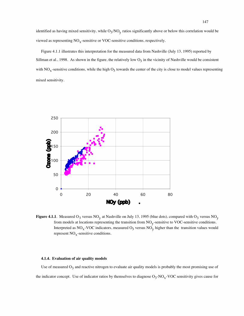
147

identified as having mixed sensitivity, while O3/NOy ratios significantly above or below this correlation would be

viewed as representing NOx-sensitive or VOC-sensitive conditions, respectively.

Figure 4.1.1 illustrates this interpretation for the measured data from Nashville (July 13, 1995) reported by

Sillman et al., 1998. As shown in the figure, the relatively low O3 in the vicinity of Nashville would be consistent

with NOx-sensitive conditions, while the high O3 towards the center of the city is close to model values representing

mixed sensitivity.

0

50

100

150

200

250

0 20 40 60 80

NOy (ppb) .

Ozo

ne (

ppb)

Figure 4.1.1. Measured O3 versus NOy at Nashville on July 13, 1995 (blue dots), compared with O3 versus NOyfrom models at locations representing the transition from NOy-sensitive to VOC-sensitive conditions.Interpreted as NOx-VOC indicators, measured O3 versus NOy higher than the transition values wouldrepresent NOx-sensitive conditions.

4.1.4. Evaluation of air quality models

Use of measured O3 and reactive nitrogen to evaluate air quality models is probably the most promising use of

the indicator concept. Use of indicator ratios by themselves to diagnose O3-NOx-VOC sensitivity gives cause for

148

doubt because it is not certain whether the correlation between indicator ratios and NOx-VOC sensitivity is

universally valid. Use of measured species to evaluate model scenarios should remain valid even if the correlation

between indicators and NOx-VOC sensitivity is less than perfect.

An evaluation of models using measured reactive nitrogen should include the following steps:

Adjustment of model boundary values: When air quality models are used to evaluate conditions in individual

metropolitan areas, they often include adjustments to O3 along the model boundary in order to reflect transport into

the area. Typically, concentrations of HNO3 and organic nitrates are set to zero along the model boundary. This

can be the cause of poor performance for indicator ratios (see Section 3.1.5) but it can also cause disagreement

between model and measured correlations among ozone and reactive nitrogen. Measurements, e.g. Trainer et al.,

1993, show that elevated O3 is also associated with elevated reactive nitrogen.

To correct this problem, model boundary conditions for PAN and HNO3 should be added based on the assumed

O3. PAN and HNO3 at the boundary should be set based on the correlations between O3 and HNO3 and between

O3 and organic nitrates shown in Figures 3.1.7 and 3.1.12.

Direct comparison between model and measured correlations: The model and measured correlation between

O3 and NOy, etc. for the afternoon hours should be compared directly as shown in Figure 3.1.9.

Model values for this comparison should be taken from locations corresponding to the array of measurement

sites. It is also useful to compare the measured correlation to model values for the entire domain, as a way of

identifying varied conditions at sites not included in the measurements.

Model versus measurement statistics: A formal comparison would use the following statistics for comparison

between models and measurements:

(i) O3, NOy and O3/NOy ratio (or equivalent with NOz and HNO3) for all model values of O3 within 10

ppb of the model maximum, and for all measured values of O3 within 10 ppb of the measured

maximum. Measurements should be within 25% of model values.

(ii) O3, NOy and O3/NOy ratio (or equivalent with NOz and HNO3) for all model values of O3 above 80

ppb, and for all measured values of O3 above 80 ppb. Specific statistics for this comparison should be

developed, (e.g. number of hours with O3/NOy at certain values).

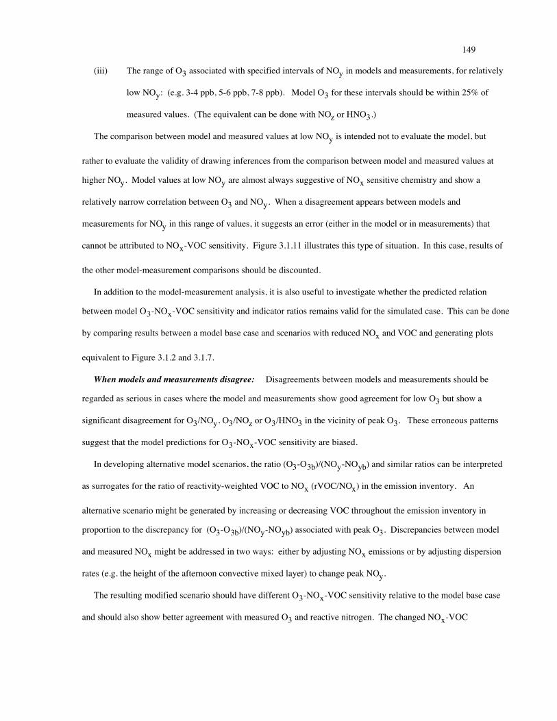
149

(iii) The range of O3 associated with specified intervals of NOy in models and measurements, for relatively

low NOy: (e.g. 3-4 ppb, 5-6 ppb, 7-8 ppb). Model O3 for these intervals should be within 25% of

measured values. (The equivalent can be done with NOz or HNO3.)

The comparison between model and measured values at low NOy is intended not to evaluate the model, but

rather to evaluate the validity of drawing inferences from the comparison between model and measured values at

higher NOy. Model values at low NOy are almost always suggestive of NOx sensitive chemistry and show a

relatively narrow correlation between O3 and NOy. When a disagreement appears between models and

measurements for NOy in this range of values, it suggests an error (either in the model or in measurements) that

cannot be attributed to NOx-VOC sensitivity. Figure 3.1.11 illustrates this type of situation. In this case, results of

the other model-measurement comparisons should be discounted.

In addition to the model-measurement analysis, it is also useful to investigate whether the predicted relation

between model O3-NOx-VOC sensitivity and indicator ratios remains valid for the simulated case. This can be done

by comparing results between a model base case and scenarios with reduced NOx and VOC and generating plots

equivalent to Figure 3.1.2 and 3.1.7.

When models and measurements disagree: Disagreements between models and measurements should be

regarded as serious in cases where the model and measurements show good agreement for low O3 but show a

significant disagreement for O3/NOy, O3/NOz or O3/HNO3 in the vicinity of peak O3. These erroneous patterns

suggest that the model predictions for O3-NOx-VOC sensitivity are biased.

In developing alternative model scenarios, the ratio (O3-O3b)/(NOy-NOyb) and similar ratios can be interpreted

as surrogates for the ratio of reactivity-weighted VOC to NOx (rVOC/NOx) in the emission inventory. An

alternative scenario might be generated by increasing or decreasing VOC throughout the emission inventory in

proportion to the discrepancy for (O3-O3b)/(NOy-NOyb) associated with peak O3. Discrepancies between model

and measured NOx might be addressed in two ways: either by adjusting NOx emissions or by adjusting dispersion

rates (e.g. the height of the afternoon convective mixed layer) to change peak NOy.

The resulting modified scenario should have different O3-NOx-VOC sensitivity relative to the model base case

and should also show better agreement with measured O3 and reactive nitrogen. The changed NOx-VOC

150

predictions should be interpreted as a measure of the level of uncertainty in those predictions. The modified

scenario might also be tested against observed VOC and NOx if such measurements are available.


1. Quality assurance: Plot measured O3 versus NOy (and, if available, O3 versus NOz and O3 versus

HNO3) for the hours 1-5pm in comparison with the model correlation for NOx-sensitive locations only

in 3.1.7. Measured ensembles are judged as valid for the indicator method if O3/NOy values are equal

to or lower than the model correlation for NOx-sensitive locations.

2. Numerical quality assurance: Identify median and 75th percentile values of O3 associated with low

ranges of NOy (2-4 ppb, 4-6 ppb, 6-8 ppb) and compare with model values for NOx-sensitive locations

in Figure 3.1.7. Measured 75th percentile O3 should be no more than 25% higher than model O3 for the

given range of NOy.

3. NOx-VOC evaluation: Plot measured O3 versus NOy, etc. for the hours 1-5pm in comparison with the

model correlation for locations with mixed sensitivity in Figure 3.1.7. Measured values higher than the

mixed-sensitivity values are interpreted as representing NOx-sensitive conditions and model values

lower than the mixed-sensitivity values are interpreted as representing VOC-sensitive conditions.

4. NOx-VOC numerical evaluation: Identify measured O3/NOy or (O3-O3b)/(NOy-NOyb), etc. for peak

O3 (1-5 pm only) during each event of interest, and identify the range of measured values for O3 greater

than 85 ppb, in comparison with the ratio values identified in Section 3.1.1. as representing the

transition value for NOx-sensitive versus VOC-sensitive photochemistry.

5. Evaluation of air quality model: Plot model O3 versus NOy (1-5 pm) for the ensemble of locations

corresponding to measured values, in comparison of measurements. Identify model ratios as in Step 4

and compare with measured values. A satisfactory model should have ratios within 25% of measured

values. (A similar test can be done using model values for the full domain.)

4.2 CONSTRAINED STEADY STATE WITH MEASURED NOx AND VOC

4.2.1. Required measurements

The method requires speciated VOC measurements, including a reasonably complete representation of directly

emitted VOC, and measured NOx. These must include the major biogenic species (isoprene). Secondary species

151

(aldehydes, biogenic reaction products) may be useful, but these are not necessary. Measured photolysis rates are

also useful but not necessary.

It is critical that the measured VOC and NOx are acceptable in terms of accuracy, and that any biases (e.g.

missing VOC species) are accounted for in the analysis. The existing PAMS network may need to be improved to

correct previously identified errors, as described in Parrish et al. (1998) and Cardelino and Chameides (2001) (see

Section 3.3.6).

4.2.2. Quality assurance of measurements

Quality assurance of measured data sets can be established by examining correlations between individual VOC

species, between individual VOC and NOx, and between NOx and NOy. These correlations can be used to establish

(i) emission ratios between individual species; and (ii) analysis of apparent photochemical aging between species.

The same correlations would also be used in the analysis of measurements for content, especially with regard to

model-measurement comparisons.

Exact procedures for quality assurance, interpretation of VOC measurements and derivation of emission ratios

among species need to be established. A complete analysis might consist of the following:

• Display of correlations among individual VOC within each of three major families (alkanes, alkenes and

aromatics) relative to a reference species in each family (propane, propene and either benzene or

toluene), following the forms of Figure 3.3.4. These displays should be used to establish apparent

emission ratios among species. As shown in Figure 3.3.4, the line representing the maximum ratio of a

short-lived to a long-lived species represents the apparent emissions ratio.

• Display of correlations of representative VOC from each family relative to a single reference species

(propane), in order to identify emission ratios.

• Comparison of the above results for early morning (6-9am) and midday/afternoon (11-5pm) to identify

differences related to photochemical aging.

• Comparison of derived emission ratios among species with prior measurements that represent typical

emission ratios among species in the U.S., with emission ratios from inventories for the metropolitan

area, and with emission ratios associated with automobile exhaust. (The latter is intended to identify

152

measurement that may be dominated by fresh auto emissions.) Table 4.2.1 provides a summary of prior

measurements.

• Display of the correlation between isoprene and a representative anthropogenic VOC (e.g. propane)

during midday and early afternoon (12-3pm), which corresponds to the time of peak isoprene, and

display of the isoprene diurnal profile.

• If NOy is available, the correlations between NOx and NOy, between O3 and NOx and between O3 and

NOz should be displayed, in order to establish whether measured NOx can be regarded as true NOx or

whether it also includes PAN. Correlations of O3 versus NOx and O3 versus NOz can be compared

with patterns from models or with research-grade measurements (see Section 4.1.1)

This may be well beyond the scope of regulatory analysis. However, a reasonable short summary might be done

by deriving emission ratios for the major VOC reactivity classes, based on measured correlations, and comparing

these ratios with inventory values. When emission ratios derived from measurements differ substantially from the

expected emission rates, a judgement would need to be made whether the results represent true ambient conditions,

measurement errors, or the impact of direct emissions (typically, auto exhaust) at the measurement site.

A separate analysis should identify VOC species that appear to be missing from the measurements, and adjust the

total measured VOC to account for the missing species.

Quality assurance for biogenic species is more difficult because no correlation is expected between biogenic

VOC and anthropogenic species. The correlation between the two major biogenic VOC (isoprene and a-pinene)

might be used for quality assurance, but deviations from expected values are more likely due to the minor species

(a-pinene) rather than to isoprene. The results for isoprene can be interpreted only in comparison with predicted

correlations and diurnal profiles from 3-d models. Individual judgment will be necessary to decide whether

discrepancies reflect errors in emission inventories rather than model dispersion rates or measurement error.

153

Table 4.2.1

Measured concentrations of hydrocarbons

Median concentrations are shown of the 48 most abundant ambient air hydrocarbons in 39 U.S. cities. Reported by

Parrish et al. (1998) from Seila et al. (1989).

4.2.3. Interpretation of measured results

Interpretation of measured VOC and NOx includes two components: (i) application and interpretation of results

from constrained steady state calculations; and (ii) derivation of emission rates based on measured correlations

among VOC and NOx.

Results of constrained steady-state calculations: Three different methods have been used to display results from

constrained steady-state calculations. Cardelino and Chameides (1995) simply reported the summed impact of

reduced NOx and reduced VOC on ozone production, where ozone production was summed over 12 hours on a

single day, and included summed values for several measurement sites that represented conditions for a given

154

metropolitan area. Tonnesen and Dennis (2000a) presented graphs that showed the predicted change in ozone

production due to changed NOx and VOC at each individual hour and each location, plotted against a proposed

indicator for instantaneous chemistry based on reactivity-weighted VOC and NOx. Kleinman et al. (1997, 2000,

2001) also showed the predicted change in ozone production rates at individual times and locations, plotted against

the parameter LN/Q which explained NOx-VOC chemistry. Kleinman et al. compared patterns for different

locations, which often had different NOx-VOC sensitivity but the same relation between NOx-VOC sensitivity and

the parameter LN/Q. The results from Kleinman et al. were the only results based on measurements. The results

shown by Cardelino and Chameides (1995) were based on pseudo-data derived from a 3-d air quality model.

Similarly, the results from Tonnesen and Dennis (2000a) represented predictions from an AQM.

For regulatory purposes it is useful to show how the predicted sensitivity to NOx and VOC is related to the rate

of ozone production (PO3) and how it varies with geography. NOx-VOC sensitivity is most important during

periods of high ozone production. This is accomplished in part by summing PO3 over extended time periods and by

representing the impact of reduced NOx and reduced VOC based on the summed impact over time, as done by

Cardelino and Chameides (1995).

The following display is suggested: diurnal sums of the impact of reduced NOx and VOC, plotted against the

equivalent sum of PO3, from measurements collected over a season, and separate sums for different geographical

locations within a metropolitan area. The summed impact of reduced NOx and VOC on ozone production, as used

by Cardelino and Chameides (1995), provides a convenient single-number summation. The summed ratio of

reactivity-weighted VOC to NOx (rVOC/NOx) summed over the midday hours associated with maximum ozone

production (10am-4pm) also provides a useful summary of measurements, because this ratio is closely associated

with NOx-VOC sensitivity. This sum must be done for midday rather than morning, because midday values include

the impact of biogenic VOC and because midday values represent conditions at the time of maximum ozone

production.

The relative impact of anthropogenic versus biogenic VOC is also of interest to the regulatory community. This

can be represented by displaying the ratio of biogenic to anthropogenic VOC, expressed either as ratio of reactivity-

weighted sums or a ratio of ozone formation potentials (Carter, 1994, 1995), plotted versus PO3. A single-number

summation can be developed by calculating the weighted sums of biogenic and anthropogenic VOC, weighted both

155

by reactivity (or by ozone formation potentials) and by the calculated rate of ozone production at the time of the

observation.

Derived emission rates: The other major result of this analysis consists of inferred emission rates for

anthropogenic VOC and NOx in comparison with emission inventories. The correlations between measured VOC

species, suggested as part of quality assurance (Section 4.2.2) also provide an effective way of displaying results of

the analysis that have implications for the regulatory process. Derived emission rates and ratios provide single-

number summations of these results.

4.2.4. Evaluation of air quality models

Constrained steady state calculations and associated NOx and VOC measurements can be used to evaluate air

quality models in two ways: direct comparisons between model and measured values or between values derived

from AQMs and from constrained steady state calculations; and evaluation of emission inventories.

In both cases, adjustment of AQMs to improve agreement with measured values will require changes in emission

rates. The measured NOx and VOC are controlled largely by these rates.

Comparison between model and measured values: Evaluation of an AQM using results of constrained steady

state calculation can be done most efficiently by deriving predicted species concentrations from the AQM that

correspond to the times and locations of available measurements. These model values can then be regarded as

pseudo-data and used to drive the equivalent CSS calculation. Assuming that CSS uses the same photochemical

mechanism as the AQM, comparison between CSS results based measurements and CSS results based on AQM

species concentrations provides an estimate of the impact of model-measurement differences on NOx-VOC

predictions.

The summed impact of reduced NOx and VOC on ozone production at the measurement sites, used by Cardelino

and Chameides (1995) as a single-number summation of results from the CSS calculation, also provides a

convenient summation of the extent of agreement between the AQM and measured NOx and VOC.

A direct comparison between model and measured values for the ratio rVOC/NOx(including both morning and

midday values) is also a useful way to summarize model performance and bias with regard to measured NOx and

VOC.

156

The ratio of summed biogenic and anthropogenic VOC concentrations, each weighted by reactivity and by rate of

ozone production coincident with the measurement (or with pseudo-data from the AQM) provides a simple estimate

of impact of biogenic VOC in the AQM in comparison with measurements.

Evaluation of emission inventories: Model emission inventories can be adjusted in two ways. Ratios of

emission inventories derived from the graphical display of measurements can be used to adjust emission rates

throughout a metropolitan area, by adjusting emission rates throughout by a constant factor. Separate adjustment

factors may be applied for geographical subregions with different emissions characteristics, based on results at

different measurement sites. An alternative method is to use inverse modeling procedures (Mendoza-Dominguez

and Russell, 2000, 2001, 2002).

It is also useful to display the predicted values of correlations between individual VOC, as described in Section

4.2.2, in comparison with measured values. Comparisons between predicted correlations from AQMs and measured

values will clearly identify the extent of agreement or disagreement.

As described in Section 4.2.2, emission rates for biogenic species cannot be derived directly from correlations

among measured species. Evaluation of biogenic emission rates is possible through model-measurement

comparisons for (i) diurnal concentration profiles, and (ii) averaged midday and afternoon concentrations (11am-

3pm) for equivalent model and measured locations. The midday and afternoon period is recommended as the time

period associated both with maximum photochemical activity and maximum impact of biogenic species.


1. Derive emission rates of all major anthropogenic VOC based on measured correlations between

individual VOC. Compare the derived emission rates with rates from emission inventories used in air

quality models. The comparison should be expressed as reactivity-weighted sums of VOC species

associated with major VOC categories, and as reactivity-weighted sums of all anthropogenic VOC. The

measurement-based emission rates are derived from species correlations between each VOC and a

reference VOC (propane), and between propane and NOy in order to derive ratios for rVOC/rNOx.

Suggested numerical procedure: identify a sequence of intervals for the measured values of the

reference VOC (propane); identify near-maximum (90th percentile) measured value other VOC species

157

for each interval value of the (slower-reacting) reference VOC; and interpret the slope between near-

maximum values and reference value as the ratio of emissions.

2. Quality assurance: Compare derived emission rates with emission rates from inventories. In cases of

major discrepancies, a judgment must be made whether the measured value or inventory value is

correct. In cases where species appear to be missing from measurements, the measurements should be

supplemented with inferred concentrations of missing VOC.

3. NOx-VOC evaluation: either

(i) Calculate ozone production based on measurements (including adjustment from #2) using the

constrained steady state model, and plot ozone production (PO3) versus calculated impact of reduced

NOx and reduced VOC; or

(ii) Plot reactivity-weighted VOC (rVOC) versus NOx (rNOx) at measurement sites associated with

urban and regional ozone production, averaged over the hours of maximum ozone production (10am-

4pm). The rVOC versus NOx can be interpreted in comparison with the values of rVOC/rNOx

associated with NOx-sensitive and VOC-sensitive instantaneous chemistry (Section 3.3.4).

NOx-VOC numerical evaluation. High and low measured rVOC/rNOx shows the approximate extent of

NOx-sensitive and VOC-sensitive photochemical production in the region.

4. Numerical NOx-VOC evaluation: either

(i) Report the summed PO3 and summed change in PO3 associated with either reduced NOx or VOC

using the constrained steady state model, following the procedures recommended by Cardelino and

Chameides (1995) (see Section 3.3.3) for an indivudal event; or

(ii) Report the average rVOC/rNOx for the event, based on summed rVOC and rNOx summed

individually over the hours of maximum ozone production (10am-4pm) at measurement sites associated

with urban and regional ozone production. Approximate NOx-VOC sensitivity is inferred based on the

correlation between sensitivity and rVOC/rNOx from Section 3.3.4.

5. Evaluation of air quality model: Repeat steps #3 and #4 using VOC and NOx concentrations from air

quality model scenarios in place of measurements. The difference between results from models and

measurements gives an indication of possible bias in NOx-VOC predictions from models. Differences

158

between emission rates inferred from models and rates from emission inventories (step #1) also provides

an evaluation of possible bias in model scenarios.

159

SECTION5. RECOMMENDATIONS FOR FURTHER RESEARCH

The research topics discussed below address two broad issues:

• Research designed to evaluate the accuracy of a proposed OBM

• Research designed to develop standard procedures for using an OBM to derive results useful in a

regulatory context. This also includes work to establish measurement networks with sufficient

accuracy.

5.1. NOx-VOC indicators

These recommendations are also useful in connection with smog production algorithms.

1. Expansion of the PAMS network to include NOy measurements of sufficient accuracy, based on

recommendations from McClenny et al. (2000).

2. Evaluation of correlations between O3 and individual reactive nitrogen species (PAN, HNO3, and other

organic nitrates) in comparison with predictions of AQMs using various photochemical mechanisms.

This should lead to an understanding concerning the relative amount of HNO3 and organic nitrates

predicted by the various photochemical mechanisms (including SAPRC 99, as the mechanism with the

most complete speciation, and CB-IV, as the mechanism most commonly used in regulatory

applications).

3. Development of a data base of correlations between O3 and NOy, O3 and NOz, O3 and HNO3 and O3

versus PAN from research-grade measurements, preferably from measurements that have been

published in scientific literature. This should include identification of different patterns in locations

with different probable NOx-VOC sensitivity. Research-grade measurements of these species have

been made in Nashville, New York, Philadelphia, Houston and Los Angeles. These measurements

should be compared and reported in a way that can be used for evaluating the accuracy of measurements

used during regulatory studies.

160

4. Development of an equivalent data base of correlations between O3 and reactive nitrogen from PAMS

and other networks used in regulatory studies, and evaluation in comparison with research-grade

measurements.

5. Comparison of proposed indicator ratios (O3/NOy, O3/NOz, O3/HNO3) and related ratios (O3/PAN) in

identical calculations using different photochemical mechanisms. This should also include comparisons

of ratios of production rates for ozone and NOz, ozone and HNO3, etc. for different amounts of VOC,

NOx and for different VOC species.

6. Evaluation of photochemical mechanisms in comparison with smog chamber experiments that include

specific transitions between NOx-sensitive and VOC-sensitive conditions. Experiments associated with

the smog production algorithms are especially useful in this regard. Measured values of proposed

indicator ratios in these experiments should be compared with values in equivalent photochemical

calculations.

5.2. Constrained steady state/measured NOx and VOC

1. The quality of measured NOx and VOC at PAMS measurement sites may need to be upgraded to correct

problems cited by Parrish et al. (2000) and Cardelino and Chameides (2000).

2. A software package should be developed for evaluating measured VOC and NOx from the PAMS

network, in close association with established protocols for reporting of PAMS data. This package

should display a standard set of correlations among individual VOC and derive emissions ratios among

VOC, following procedures used by Goldan et al. (1995) and Parrish et al. (1998, 2000). The package

should include display of these derived emission ratios in comparison with U.S. averages and in

comparison with fresh auto exhaust. Other standard tests for quality assurance could be included. The

same software package can include the constrained steady state calculation for clear-sky conditions and

display standard output.

3. Associated with the above recommendation, a series of standard tests for quality assurance of measured

VOC, standard methods for display of results from measurements pertaining to anthropogenic and

biogenic VOC inventories, and standard methods for reporting and interpreting results of constrained

steady state calculations need to be developed.

161

4. The representation of the vertical distribution of directly emitted VOC in the current generation of air

quality models needs to be investigated. This is especially important for highly reactive species (e.g.

isoprene) during typical daytime conditions with rapid convective mixing. The rate of dispersion out of

the surface layer in AQMs may have a significant impact on model species concentrations. Model

vertical profiles of isoprene can be compared with measured profiles reported by Andronache et al.

(1994) and Guenther et al. (1996a, 1996b). For other species, vertical profiles in regions with high

direct emission rates need to be measured.

162

SECTION 6. REFERENCES

Andronache, C., W. L. Chameides, M. O. Rodgers, J. E. Martinez, P. Zimmerman, and J. Greenberg. Verticaldistribution of isoprene in the lower boundary layer of the rural and urban southern United States. J. Geophys.Res., 99,16989-17000, 1994.

Blanchard, C. L., and D. Fairley. Spatial mapping of VOC and NOx-limitation of ozone formation in centralCalifornia. Atmos. Environ. 2001, In press.

Blanchard, C. L. Spatial Mapping of VOC and NOx Limitation of Ozone Formation in Six Areas. 92nd AnnualMeeting of the Air and Waste Management Association, Orlando, Florida. June 24-28, 2001; paper no.. 21, sessionno. AB-2c.

Blanchard, C. L., and T. Stoeckenius, Ozone response to precursor controls: comparison of data analysis methodswith the predictions of photochemical air quality simulation models. Atmos. Environ., 35, 1203-1216, 2001.

Blanchard, C. L., Ozone process insights from field experiments- Part III: Extent of reaction and ozone formation.Atmos. Environ. 2000, 34: 2035-2043.

Blanchard, C. L., F. W. Lurmann, P. M. Roth, H. E. Jeffries, and M. Korc, The use of ambient data to corroborateanalyses of ozone control strategies, Atmos. Environ., 33, 369-381, 1999.

Blanchard, C. L., P. T. Roberts, L. R. Chinkin, and P. M. Roth. Application of smog production (SP) algorithms tothe TNRCC COAST data. 86th Annual Meeting of the Air and Waste Management Association, San Antonio,Texas. 1995; paper 95_TP15P.04.

Blanchard, C. L., Spatial Mapping of VOC and NOx Limitation of Ozone Formation in Six Areas. 92nd AnnualMeeting of the Air and Waste Management Association, Orlando, Florida. June 24-28, 2001; paper no. 21,session no. AB-2c.

Bowen, J. L. and I. Valiela, Historical changes to atmospheric nitrogen deposition to Cape Cod, Massachusetts,USA., Atmos. Environ., 35, 1039-1051, 2001.

Buhr, M., D Parrish, J. Elliot, J. Holloway, J. Carpenter, P. Goldan, W. Kuster, M. Trainer, S. Montzka, S. McKeen,and F. C. Fehsenfeld, Evaluation of ozone precursor source types using principal component analysis ofambient air measurements in rural Alabama. J. Geophys. Res., 100, 22853-22860, 1995.

Buhr, M. P., M. Trainer, D. D. Parrish, R. E. Sievers, and F. C. Fehsenfeld, Assessment of pollutant emissioninventories by principal component analysis of ambient air measurements, Geophys. Res. Letters, 19, 1009-1012, 1992.

Butler, T. J., G. E. Likens and .B. J. B. Stunder, Regional-scale impacts of Phase I of the Clean Air ActAmendments in the USA: the relation between emissions and concentrations, both wet and dry, Atmos.Environ., 35, 6, 1015-1028, 2001.

Cardelino, C. and W. L. Chameides. An observation-based model for analyzing ozone-precursor relationships in theurban atmosphere. J. Air Waste Manage. Assoc., 45, 161-180, 1995.

Cardelino, C. A. and W. L. Chameides, The application of data from photochemical assessment monitoring stationsto the observation-based model, Atmos. Environ., 34, 2325-2332, 2000.

163

Carroll, M.A., D. R. Hastie, B. A. Rdley, M. O. Rodgers, A. L. Torres, D. D. Davis, J. D. Bradshaw, S. T.Sandholm, H. I. Schiff, D. R. Karecki, G. W. Harris, G. I. Mackay, G. L. Gregory, E. P. Condon, M.Trainer, G. Hubler, D. D. Montzka S. Madronich, D. L. Albritton, H. B. Singh, S. M. Beck, M. C. Shipham,and A. S. Bachmeier, Aircraft measurements of NOx over the eastern Pacific and continental United States andimplications for ozone production. J. Geophys. Res., 95, 10199-10204 1990.

Chin, M., D. J. Jacob, J. W. Munger, D. D. Parrish and B. G. Doddridge, Relationship of ozone and carbonmonoxide over North America. J. Geophys. Res., 99, 14565-14573, 1994.

Carter, W. P. L. Development of ozone reactivity scales for volatile organic compounds, J. Air Waste Manage.Assoc., 44, 881-899, 1994.

Carter, W. P. L., Computer modeling of environmental chamber studies of maximum incremental reactivities ofvolatile organic compounds, Atmos. Environ., 29-18, p. 2513, 1995.

Chameides, W. L., F. Fehsenfeld, M. O. Rodgers, C. Cardellino, J. Martinez, D. Parrish, W. Lonneman, D. R.Lawson, R. A. Rasmussen, P. Zimmerman, J. Greenberg, P. Middleton, and T. Wang, Ozone precursorrelationships in the ambient atmosphere. J. Geophys. Res., 97, 6037-6056, 1992.

Chang, M. E., D. E. Hartley, C. Cardelino, D. Hass-Laursen, and W. L. Chang, On using inverse methods forresolving emissions with large spatial inhomogeneities, J. Geophys. Res., 102, 16023-16036, 1997.

Chang, M. E., C. Cardelino, d. Hartley, and W. L. Chang, Inverse modeling of biogenic emissions, Geophys. Res.,Lett., 3, 3007, 1996.

Chang, T. Y., D. P. Chock, B. I. Nance, and S. L. Winkler. A photochemical extent parameter to aid ozone airquality management. Atmos. Environ., 31, 2787-2794, 1997.

Chang, T. Y. and M. Suzio: "Assessing Ozone-Precursor Relationships Based on Smog Production Model andAmbient Data." J. Air & Waste Manage. Assoc. 45, 20-28 (1995).

Chang, T. Y. and M. Suzio: "A Smog Production Model and An Assessment of Ozone Control Strategies."Prodeedings of the 1994 AWMA Conference on Tropospheric Ozone: Critical Issues in the Regulatory Process.Air and Waste Management Association, Pittsburgh, PA 15222, pp. 550-561 (1996).

Cheng, M-D., P. K. Hopke, and Y. Zeng, A receptor-oriented methodology for determining source regions ofparticulate sulfate observed at Dorset, Ontario, J. Geophys. Res., 98, 16839-16849, 1993.

Chin, M., D. J. Jacob, J. W. Munger, D. D. Parrish and B. G. Doddridge, Relationship of ozone and carbonmonoxide over North America. J. Geophys. Res., 99, 14565-14573, 1994.

Chock, D. P., T. Y. Chang, S. L. Winkler, and B. I. Nance, The impact of an 8 h ozone air quality standard onROG and NOx controls in Southern California. Atmos. Environ., 33, 2471-2486, 1999.

Clark, T. L. and T. R. Karl, Application of prognostic meteorological variables to forecasts of daily maximum one-hour ozone concentrations in the northeastern United States, J. Appl. Meteo., 21, 1662-1671, 1982.

Collins, W. J., D. S. Stevenson, C. E. Johnson, and R. G. Derwent, The European regional ozone distribution andits links with the global scale for the years 1992 and 2015, Atmos. Environ., 34, 255-267, 2000.

Daum, P. H., L. Kleinman, D. G. Imre, L. J. Nunnermacker, Y.-N. Lee, S. R. Springston, and L. Newman,Analysis of the processing of Nashville urban emissions on July 3 and July 18, 1995, J. Geophys. Res., 105.9155-9164, 2000.

164

Dommen, J, A. S. H. Prevot, A. M. Hering, T. Staffelbach, G. L. Kok, and R. D. Schillawski, Photochemicalproduction and the aging of an urban air mass. J. Geophys. Res., 104, 5493-5506, 1999.

Fenger, J., Urban air quality. Atmos. Environ., 33, 4877-4900, 1999.

Fiore, A. M., D. J. Jacob, J. A. Logan, and J. H. Yin, Long-term trends in ground level ozone over the contiguousUnited States, 1980-1995. J. Geophys. Res., 103, 1471-1480, 1998.

Fiore, A. M., D. J. Jacob, I. Bey, Y. M. Yantoska, B. D. Field, A. C. Fusco, and J. G. Wilkensen, Backgroundozone over the United States in summer: origin, trend, and contribution to pollution episodes. J. Geophys.Res., in press, 2002 (available at http://www-as.harvard.edu/chemistry/trop/recentpapers.html).

Fujita, E. M., B. E. Croes, C. L. Bennett, D. R. Lawson, F. W. Lurmann and H. H. Main, Comparison of emissionand ambient concentration ratios of CO, NOx, and NMOG in California's south coast air basin. J. Air WasteMgmt. Assoc., 42:264-276 1992.

Geron, C. D., A. B. Guenther, and T. E. Pierce. An improved model for estimating emissions of volatile organiccompounds from forests in the eastern United States. J. Geophys. Res., 99, 12773-12791, 1994.

Gery, M. W. G. Z. Whitten, J. P. Killus and M. C. Dodge. A photochemical kinetics mechanism for urban andregional computer modeling. J. Geophys. Res., 94, 12925-12956, 1989.

Gillani, N. V. and J. E. Pleim. Sub-grid-scale features of anthropogenic emissions of NOx and VOC in the contextof regional Eulerian models. Atmos. Environ., 30, 2043-2059, 1996.

Gilliland, A., and P. Abbitt, A sensitivity study of the discrete Kalman filter (DKF) to initial conditiondiscrepancies, J. Geophys. Res., 106, 17939-17952, 2001.

Goldan, P. D., M. Trainer, W. C. Kuster, D. D. Parrish, J. Carpenter, J. M. Roberts, J. E. Yee, and F. C. Fehsenfeld.Measurements of hydrocarbons, oxygenated hydrocarbons, carbon monoxide and nitrogen oxides in an urbanbasin in Colorado: implications for emissions inventories. J. Geophys. Res., 100, 22771-22785, 1995.

Goldan, P. D., W. C. Kuster, and F. C. Fehsenfeld, Non-methane hydrocarbon measuremetns during thetropospheric OH photochemistry experiment, J. Geophys. Res., 102, 6315-6324, 1997.

Goldan, P. D., D. D. Parrish, W. C. Kuster, M. Trainer, S. A. McKeen, J. Holloway, B. T. Jobson, D. T. Sueper,and F. C. Fehsenfeld, Airborne measurements of isoprene, CO and anthropogenic hydrocarbons and theirimplications, J. Geophys. Res., in press, 2001.

Goldstein, A. H., and G. W. Schade, Quantifying biogenic and anthropogenic contributions to acetone mixingratiosin a rural environment, Atmos. Environ., 34, 4997-5006, 2000.

Guenther, A., P. Zimmerman, L. Klinger, J. Greenberg, C. Ennis, K. Davis, W. Pollock, H. Westberg, G. Allwine,and C. Geron, Estimates of regional natural volatile organic compound fluxes from enclosure and ambientmeasurements. J. Geophys. Res., 101, 1345-1359, 1996a.

Guenther, A., W. Baugh, K. Davis, G. Hampton, P. Harley, L. Klinger, L. Vierling, P. Zimmerman, E. Allwine, S.Dilts, B. Lamb, H. Westberg, D. Baldocchi, C. Geron, and T. Pierce, Isoprene fluxes measured by enclosure,relaxed eddy accumulation, surface layer gradient, mixed layer gradient, and mixed layer mass balancetechniques. J. Geophys. Res., 101, 18555-18567, 1996b.

Hammer, M.-U., B. Vogel, and H. Vogel, Findings on H2O2/HNO3 as an Indicator of Ozone Sensitivity in Baden-Württemberg, Berlin-Brandenburg, and the Po Valley Based on Numerical Simulations, J. Geophys. Res., inpress, 2001.

165

Harley, R. A., R. F. Sawyer, J. B. Milford, Updated photochemical modeling for California's South Coast airbasin: comparison of chemical mechanisms and motor vehicle emission inventories. Enviro. Sci. Tech., 31,2829-2839.

Henry, R. C., C. W. Lewis, P. K. Hopke, and H. W. Williamson, Review of receptor modeling fundamentals,Atmos. Environ., 18, 1507-1515, 1984.

Hess, G. D., F. Carnovale, M. E. Cope, and G. M. Johnson, The evaluation of some photochemical smog reactionmechanisms-I. Temperature and initial composition effects. Atmos. Environ., 26A, 625-641, 1992.

Hess, G. D., F. Carnovale, M. E. Cope, and G. M. Johnson, The evaluation of some photochemical smog reactionmechanisms-II. Initial addition of alkanes and alkenes. Atmos. Environ., 26A, 642-650, 1992.

Hess, G. D., F. Carnovale, M. E. Cope, and G. M. Johnson, The evaluation of some photochemical smog reactionmechanisms-III. Dilution and emissions effects. Atmos. Environ., 26A, 651-658, 1992.

Hirsch, A. I., J. W. Munger, D. J. Jacob, L. W. Horowitz, and A. H. Goldstein, Seasonal variation of the ozoneproduction efficiency per unit NOx at Harvard Forest, Massachusetts. J. Geophys. Res., 101, 12659-12666,1996.

Hopke, P. K., Receptor Modeling in Environmental Chemistry, John wiley, New York, New York, 1985.

Jacob, D. J., B. G. Heikes, R. R. Dickerson, R. S. Artz and W. C. Keene. Evidence for a seasonal transition fromNOx- to hydrocarbon-limited ozone production at Shenandoah National Park, Virginia. J. Geophys. Res., 100,9315-9324, 1995.

Jacob, D.J., J.A. Logan, and P.P. Murti., Effect of Rising Asian Emissions on Surface Ozone in the United States,Geophys. Res. Lett., 26, 2175-2178, 1999.

Jacobson, M. Z., R. Lu, R. P. Turco, and O. P. Toon, Development and application of a new air pollution modelingsystem-Part I: Gas-phase simulations. Atmos. Environ., 30, 1939-1963, 1996.

Jaegle, L., D.J. Jacob, W.H. Brune, D. Tan, I. Faloona, A.J. Weinheimer, B.A. Ridley, T.L. Campos, and G.W.Sachse, Sources of HOx and production of ozone in the upper troposphere over the United States, Geophys.Res. Lett., 25, 1705-1708, 1998.

Johnson, G. M., A simple model for predicting the ozone concentration of ambient air. Proc. Eighth Inter. CleanAir Confer., Melbourne, Australia, May 2, 1984, p. 715-731.

Johnson, G. M. and S. M. Quigley, A universal monitor for photochemical smog, paper 89-29.8, Air and WasteManagement Association 82nd Annual Meeting and Exhibition, Anaheim, CA, June 25-30, 1989,

Johnson, G. M., S. M. Quigley, and J. G. Smith. Management of photochemical smog using the AIRTRAKapproach. 10th International Conference of the Clean Air Society of Australia and New Zealand, Auckland,New Zealand, March, 1990, p. 209-214.

Kim, B. M. and R. C. Henry, Application of SAFER model to tbe Los Angeles PM10 data, Atmos. Environ., 34,1747-1759, 2000.

Kirchner, F., F. Jeaneret, A. Clappier, B. Kruger, H. van den Bergh, and B. Calpini, Total VOC reactivity in theplanetary boundary layer 2. A new indicator for determining the sensitivity of the ozone production to VOCand NOx, J. Geophys. Res., 106, 3095-3110, 2001.

166

Kleinman, L. H., P. H. Daum, Y-N. Lee, L. J. Nunnermacker, S. R. Springston, J. Weinstein-Lloyd, and JochenRudolph, Sensitivity of ozone production rate to ozone precursors, Geophys. Res. Lett.,28, 2903-2906, 2001,2001.

Kleinman, L. I., P. H. Daum,Y-N. Lee, L. J. Nunnermacker, S. R. Springston, J. Weinstein-Lloyd, P. Hyde, P.Doskey, J. Rudolf, J. Fast and C. Berkowitz, Photochemical age determinations in the Phoenix metropolitanarea. J. Geophys. Res., 10.1029/2002JD002621, 2003.

Kleinman, L. I., P. H. Daum, D. G. Imre, J. H. Lee, Y-N. Lee, L. J. Nunnermacker, S. R. Springston, J.Weinstein-Lloyd, and L. Newman, Ozone production in the New York City urban plume, J.Geophys. Res.,105, 14495-14511, 2000.

Kleinman, L. I., Ozone procuess insights from field experiments – part II; observation-based analysis for ozoneproduction. Atmos. Environ., 34, 2023-2034, 2000.

Kleinman, L. I., P. H. Daum, J. H. Lee, Y-N. Lee, L. J. Nunnermacker, S. R. Springston, L. Newman, J. Weinstein-Lloyd and S. Sillman. Dependence of ozone production on NO and hydrocarbons in the troposphere. Geophys.Res. Lett., 24, 2299-2302, 1997.

Kleinman, L. I., Low and high-NOx tropospheric photochemistry. J. Geophys. Res., 99, 16831-16838, 1994.

Kubler, J., H. van den Bergh, and A. G. Russell, Long-term trends of primary and secondary pollutantconcentrations in Switzerland and their response to emission controls and economic changes, Atmos. Environ.,35, 1351-1363, 2001.

Lefohn, A.S., D.S. Shadwick, S.D. Ziman, The Difficult Challenge of Attaining EPA’s new Ozone Standard,Environ. Sci. & Technol., 276A-282A, 1998.

Li, Q., et al., Transatlantic Transport of Pollution and its Effects on Surface Ozone in Europe and North America, J.Geophys. Res., in press, 2002 (available at http://www-as.harvard.edu/chemistry/trop/recentpapers.html ).

Lin, C., and J. B. Milford, Decay-adjusted chemical mass balance receptor modeling for volatile organiccompounds, Atmos Environ., 28, 3261-3276, 1994.

Lin, X., M. Trainer, and S. C. Liu, On the nonlinearity of tropospheric ozone, J. Geophys Res., 93, 15879-15888,1988.

Liu, S. C., M. Trainer, F. C. Fehsenfeld, D. D. Parrish, E. J. Williams, D. W. Fahey, G. Hubler, ad P. C. Murphy,Ozone production in the rural troposphere and the implications for regional and global ozone distributions. J.Geophys. Res., 92, 4191-4207, 1987.

Logan, J. A., Ozone in rural areas of the United States, J. Geophys. Res., 94, 8511-8532, 1989.

Lu, C-H. and J. S. Chang. On the indicator-based approach to assess ozone sensitivities and emissions features. J.Geophys. Res., 103, 3453-3462, 1998.

Luke, W. T., T. B. Wtson, K. J. Olszyna, R. Laureen Gunter, R. T. McMillen, D. L. Wellman, and S. W.Wilkison, Comparison of airborne and surface trace gas measurements during the Southern Oxidant Study, J.Geophys. Res., 103, 22317-22337, 1998.

Lurmann, F. W., and H. H. Main, Analysis of the ambient VOC data collected in the Southern California AirQuality Study, Sonoma Technology, Inc., Santa Rosa, CA, 1992.

167

Lurmann, F. W., Lloyd, A. C., and Atkinson, R. A chemical mechanism for use in long-range transport/aciddeposition computer modeling. J. Geophys. Res. 91, 10905-10936, 1986.

Martilli, A., A. Neftel, G. Favaro, F. Kirchner, S. Sillman, and A. Clappier, Simulation of the ozone formation inthe northern part of the Po Valley with the TVM-CTM. J. Geophys. Res., in press, 2001.

McClenny, W. A. ed, Recommended Methods for Ambient Air Monitoring of NO, NO2, NOy, and Individual NOzSpecies, EPA/600/R-01/005, September, 2000.

McKeen and S. C Liu, Hydrocarbon ratios and the photochemical history of air masses, Geophys. Res. Letters, 20,2363-2366, 1993.

McKeen, S. A., S. C. Liu, E.-Y. Hsie, X. Lin, J. D. Bradhaw, s. Smyth, G. L. Gregory, and D. R. Blake, 1996.Hydrocarbon ratios during PEM-WEST A: A model perspective. J. Geophys. Res., 101, 2087-2109.

McKeen, S. A., G. Mount, F. Eisele, E. Williams,J. Harder, Pl Goldan, W. Kuster, S. C. Liu, K. Baumann, D.Tanner, A. Fried, S. Sewell, C. Cantrell, and R. Shetter, Photochemical modeling of hydroxyl and itsrelationship to other species during the Tropospheric OH Photochemistry Experiment. J. Geophys. Res., 102,6467-6493, 1997.

Mendoza-Dominguez, A., J. W. Boylan, Y-J. Yang and A. G. Russell, Efficient sensitivity analysis of an air qualitymodel for primary and secondary aerosol source impact quantification, submitted to J. Geophys. Res., 2002.

Mendoza-Dominguez, A., and A. G. Russell, Estimation of emission adjustments from the application of four-dimensional data assimilation to photochemical air quality modeling, Atmospheric Environment, 35, 2879-2894, 2001.

Mendoza-Dominguez and Russell, Iterative Inverse Modeling and Direct Sensitivity Analysis of a PhotochemicalAir Quality Model, Environ. Sci. Technol., 3, 4974-4981, 2000.

Milford, J., D. Gao, S. Sillman, P. Blossey, and A. G. Russell. Total reactive nitrogen (NOy) as an indicator for thesensitivity of ozone to NOx and hydrocarbons. J. Geophys. Res. , 99, 3533-3542, 1994.

Milford, J., A. G. Russell, and G. J. McRae, A new approach to photochemical pollution control: implications ofspatial patterns in pollutant responses to reductions in nitrogen oxides and reactive organic gas emissions.Environ. Sci. Tech. 23, 1290-1301, 1989.

NARSTO. An Assessment of Tropospheric Ozone Pollution: A North American Perspective. The NARSTOSynthesis Team, July, 2000.

National Research Council (NRC), Committee on Tropospheric Ozone Formation and Measurement. Rethinkingthe Ozone Problem in Urban and Regional Air Pollution, National Academy Press, 1991.

Olszyna, K. J., E. M. Bailey, R. Simonaitis, and J. F. Meagher. O3 and NOy relationships at a rural site. J.Geophys. Res., 99, 14557-14563, 1994.

Olszyna, K. J., W. J. Parkhurst, and J. F. Meagher, Air chemistry during the 1995 SOS/Nashville intensivedetermined from level 2 network, J. Geophys. Res., 103, 31143-31153, 1998.

Oreskes, N., K. Shrader-Frechette, and K. Beliz, Verification, validation, and confirmation of numerical models inthe earth sciences, Science, 263, 641-646, 1994.

168

Parrish, D. D., M. Trainer, M. P. Buhr, B. A. Watkins, and F. C. Fehsenfeld. Carbon monoxide concentrations andtheir relation to concentrations of total reactive oxided nitrogen at two rural U.S. sites. J. Geophys. Res., 96,9309-9320, 1991.

Parrish, D. D., et al., Internal consistency tests for evaluation of measurements of anthropogenic hydrocarbons inthe troposphere, J. Geophys. Res.,, 103, 22,339-22,359, 1998.

Parrish, D.D., and F.C. Fehsenfeld, Methods for gas-phase measurements of ozone, ozone precursors and aerosolprecursors, Atmos, Environ., 34, 1921-1957, 2000.

Paulson, S. E. and J. H. Seinfeld. Development and evaluation of a photooxidation mechanism for isoprene. J.Geophys. Res., 97, 20703-20715, 1992.

Paulson, S. E. and J. J. Orlando, The reaction of ozone with alkenes: An important source of HOx in the boundarylayer, Geophys. Res. Lett., 23, 3727-3730, 1996.

Pierce, T., C. Geron, L. Bender, R. Dennis, G. Tonnesen, and A. Guenther, Influence of increasedisopreneemissions on regional ozone modeling, J. Geophys. Res.,103, 25611-25630, 1998.

Prevot, A. S. H., J. Staehelin, G. L. Kok, R. D. Schillawski, B. Neininger, T. Staffelbach, A. Neftel, H. Wernli, andJ. Dommen, The Milan photooxidant plume. J. Geophys. Res., 102, 23375-23388, 1997.

Reynolds, S., H. Michaels, P. Roth, T. W. Tesche, D. McNally, L. Gardner, and G. Yarwood, Alternative base casesin photochemical modeling: their construction, role, and value. Atmos. Environ., 30, 12, 1977-1988, 1996.

Ridley, B. A., S. Madronich, R. B. Chatfield, J. G. Walega, R. E. Shetter, M. A. Carroll, and D. D. Montzka,Measurements and model simulations of the photostationary state during the Mauna Loa ObservatoryPhotochemistry Experiment: Implications for radical concentrations and ozone production and loss rates. J.Geophys. Res., 97, 10375-10388, 1992.

Roberts, J. M., J. Williams, K. Baumann, M. P. Buhr, P. D. Goldan, J. Holloway, G. Hubler, W. C. Kuster, S.A. McKeen, T.B. Ryerson, M. Trainer, E. J. Williams, F. C. Fehsenfeld, S. B. Bertman, G. Nouaime, C.Seaver, G. Grodzinsky, M. Rodgers, and V. L. Young, Measurements of PAN, PPN , and MPAN madeduring the 1994 and 1995 Nashville Intensives of the Southern Oxidant Study: Implications for regional ozoneproduction from biogenic hydrocarbons. J. Geophys. Res., 103, 22473-22490, 1998.

Roselle, S. J. and K. L. Schere. Modeled response of photochemical oxidants to systematic reductions inanthropogenic volatile organic compound and NOx emissions. J. Geophys. Res., 100, 22929-22941, 1995.

Ryerson, T. B., M. B. Buhr, G. Frost, P. D. Goldan, J. S. Holloway, G. Hubler, B. T. Jobson, W. C. Kuster, S. A.McKeen, D. D. Parrish, J. M. Roberts, D. T. Sueper, M. Trainer, J. Williams, and F. C. Fehsenfeld, Emissionslifetimes and ozone formation in power plant plumes. J. Geophys. Res., 103, 22569-22584, 1998.

Ryerson, T. B., M. Trainer, J. S. Holloway, D. D. Parrish, L. G. Huey, D. T. Sueper, G. J. Frost, S. G. Donnelly,S. Schaufflfer, E. Atlas, W.C. Kuster, P. D. Goldan, G. Hubler, J. F. Meagher, and F. C. Fehsenfeld,Observations of ozone formation in power plant plumes and implications for ozone control strategies, Science ,292, 719-722, 2001.

Seila, R. L., W. A. Lonneman, and S. A. Meeks, Project Summary!: Determination of C2 to C12 Ambient AirHyderocarbons in 39 U.S. Cities, from 1984 through 1986, EOA Rep., EPA/600/S3-89/058, Environ. Pot.Agency, Washington, D.C., 1989.

169

Sillman, S. The use of NOy, H2O2 and HNO3 as indicators for O3-NOx-ROG sensitivity in urban locations. J.Geophys. Res., 100, 14175-14188, 1995.

Sillman, S., K. Al-Wali, F. J. Marsik, P. Nowatski, P. J. Samson, M. O. Rodgers, L. J. Garland, J. E. Martinez, C.Stoneking, R. E. Imhoff, J-H. Lee, J. B. Weinstein-Lloyd, L. Newman and V. Aneja. Photochemistry of ozoneformation in Atlanta, GA: models and measurements. Atmos. Environ., 29, 3055-3066, 1995.

Sillman, S., D. He, C. Cardelino and R. E. Imhoff. The use of photochemical indicators to evaluate ozone-NOx-hydrocarbon sensitivity: Case studies from Atlanta, New York and Los Angeles. J. Air Waste Manage. Assoc.,47, 642-652, September, 1997.

Sillman, S., D. He, M. Pippin, P. Daum, L. Kleinman, J. H. Lee and J. Weinstein-Lloyd. Model correlations forozone, reactive nitrogen and peroxides for Nashville in comparison with measurements: implications for VOC-NOx sensitivity. J. Geophys. Res. 103, 22629-22644, 1998.

Sillman, S. The method of photochemical indicators as a basis for analyzing O3-NOx-hydrocarbon sensitivity.NARSTO reviews of tropospheric ozone, available at http://www.cgenv.com/Narsto/critrev.papers.html , 2000.

Sillman, S., M. T. Odman, and A. G. Russell, Comment on "On the indicator-based approach to assess ozonesensitivities and emissions features" by C-H. Lu and J. S. Chang, J. Geophys. Res., 106 , D18 , 20,941, 2001.

Sillman, S., Comment on 'The Impact of An 8-hour Ozone Air Quality Standard on VOC and NOx Controls inSouthern California' by Chock, et al., Atmos. Environ. 35, 3370-3371, 2001.

Sillman, S., and D. He, Some theoretical results concerning O3-NOx-VOC chemistry and NOx-VOC indicators, J.Geophys. Res., 107, 10.1029/2001JD001123, ,2002.

Sillman, S., R. Vautard, L. Menut, and D. Kley, O3-NOx-VOC sensitivity and NOx-VOC indicators in Paris:results from models and ESQUIF measurements, J. Geophys. Res., in press, ,2003.

Sosa, G., J. West, F. San Martini, L. T. Molina and M. J. Molina, "Air Quality Modeling and Data Analysis forOzone and Particulates in Mexico City." MIT Integrated Program on Urban, Regional and Global Air PollutionReport No. 15, 76 pages, October 2000, available from http://eaps.mit.edu/megacities/index.html .

Staffelbach, T., A. Neftel, A. Blatter, A. Gut, M. Fahrni, J. Stahelin A. Prevot, A. Hering, M. Lehning, B. Neininger,M. Baumie, G. L. Ko, J. Dommen, M. Hutterli and M. Anklin. Photochemical oxidant formation over southernSwitzerland, part I: Results from summer, 1994. J. Geophys. Res., 102, 23345-23362, 1997.

Stockwell, W. R., F. Kirchner and M. Kuhn. A new mechanism for regional atmospheric chemistry modeling. J.Geophys. Res., 102, 25847-25879, 1997.

Stockwell, W. R., P. Middleton, J. S. Chang, and X. Tang, The second generation Regional Acid DepositionModel chemiscal mechanism for regional air quality modeling, J. Geophys. Res., 95, 16343-16367, 1990.

Tan, D., I. Faloona, W. H. Brune, P. Shepson, T. L. Couch, A. L. Sumner, T. Thornberry, M. A. Carroll, E. Apel, D.Riemer, and W. Stockwell, HOx budgets in a deciduous forest: Results from the PROPHET summer 1998campaign, J. Geophys. Res., 106, 24407-24428, 2001.Thielman, A., A. S. H. Prevot, F. C;. Gruebler, and J.Staelhelin, Empirical ozone isopleths as a tool to identify ozone production regimes, Geophys. Res. Lett., 28,2369-2372, 2001a.

Thielman, A., A. S. H. Prevot, and J. Staelhelin, Sensitivity of ozone production derived from field measurementsin the Italian Po Basin, J. Geophys. Res., in press, 2001b.

170

Thornton, J. A., P. A. Wooldridge, R. C. Cohen, M. Martinez, H. Harder, W. H. Brune, E. J. Williams, F. C.Fehsenfeld, S. R. Hall, R. E. Shetter, B. P. Wert, and A. Fried, Observations of ozone production rates as afunction of NOx abundances and HOx production rates in the Nashville urban plume, J. Geophys. Res., inpress, 2002.

Tonnesen, G. S. and R. L. Dennis, Analysis of radical propagation efficiency to assess ozone sensitivity tohydrocarbons and NOx. Part 1: Local indicators of odd oxygen production sensitivity, J. Geophys. Res., 105,9213-9225, 2000a.

Tonnesen, G. S., and R. L. Dennis, Analysis of radical propagation efficiency to assess ozone sensitivity tohydrocarbons and NOx. Part 2:Long-lived species as indicators of ozone concentration sensitivity, J. Geophys.Res., 105, 9227-9241, 2000b.

Trainer, M., D. d. Parrish, P. d. Golday, J. Roberts, and F. C. Fehsenfeld, Review of observation-based analysis ofthe regional factors influencing ozone concentrations, Atmos. Environ., 34, 2045-2061, 2000.

Trainer, M., D. D. Parrish, M. P. Buhr, R. B. Norton, F. C. Fehsenfeld, K. G. Anlauf, J. W. Bottenheim, Y.Z. Tang,H.A. Wiebe, J.M. Roberts, R.L. Tanner, L. Newman, V.C. Bowersox, J.M. Maugher, K.J. Olszyna, M.O.Rodgers, T. Wang, H. Berresheim, and K. Demerjian. Correlation of ozone with NOy in photochemically agedair. J. Geophys. Res., 98, 2917-2926, 1993.

Vogel, B., N., Riemer, H. Vogel, F. Fiedler, Findings on NOy as an indicator for ozone sensitivity based ondifferent numerical simulations, J. Geophys. Res., 3605-3620, 1999.

Watson, J. G., J. C. Chow, and E. M. Fujita, Review of volatile organic compound source apportionment bychemical mass balance, Atmos. Environ., 35, 1567-1584, 2001.

West, J. J., G. Sosa, F. San Martini, M. J. Molina, and L. T. Molina (2000) Air quality modeling and data analysisfor ozone and particulates in Mexico City, MIT-IPURGAP Report No. 15, 76 pages, Oct. 2000.

Wild, O., and H. Akimoto, Intercontinental transport of ozone and its precursors in a three-dimensional global CTM,J. Geophys. Res., 106, 27,729-27,744, 2001.

Williams, E. J., K. Baumann, J. M. Roberts, S. B. Bertman, R. B. Norton, F.C. Fehsenfeld, S. R. Springston, L.J. Nunnermacker, L. Newman, K. Olszyna, J. Meagher, B. Hartsell, E. Edgerton, J. R. Pearson, and M. O.Rodgers, Intercomparison of ground-based NOy measurement techniques, J. Geophys. Res., 103, 22261-22280, 1998.

Winer, A. M., J. W. Peters, J. P. Smith, and J. N. Pitts, Jr. Response of commercial chemiluminescent NO-NO2analyzers to other nitrogen-containing compounds. Environ. Sci. Technol. 1974, 8:1118-1121.

Winkler, S. L. and D.P. Chock: "Reply on Comment on 'The Impact of An 8-hour Ozone Air Quality Standard onVOC and NOx Controls in Southern California' by Chock, et al." Atmos. Environ. 35, 3371-3372 (2001).

Yienger, J.J., et al., The episodic nature of air pollution transport from Asia to North America, J. Geophys. Res.,105, 26,931-26,945, 2000.

171

APPENDIX: ADDITIONAL RESULTS FOR NOx-VOC INDICATORS

This section includes (i) a statistical representation of indicator values associated with NOx-sensitive and VOC-

sensitive locations in individual photochemical models; and (ii) complete graphical representation of material from

Section 3.1.1.

Numerical summary of indicator results: Sillman (1995) and Sillman et al. (1998) developed the following as

a convenient method to summarize information contained in indicator NOx-VOC sensitivity graphs (see Figure 3.1.1

and 3.1.2).

The summary information consists of the following: The distribution of indicator values is identified for (i) all

locations with NOx-sensitive conditions in an individual model scenario; and (ii) all locations with VOC-sensitive

conditions for the scenario. The distribution of NOx-sensitive and VOC-sensitive indicator values is then

summarized by identifying (i) the 5th-percentile valne; (ii) the median (50th percentile) value; and (iii) the 95th-

percentile value.

Model results that show a strong separation of between NOx-sensitive and VOC-sensitive values have the

following characteristics: median values associated with NOx-sensitive and VOC-sensitive conditions differ from

each other by at least a factor of 2; and the 95th percentile value for VOC-sensitive conditions is typically equal to or

lower than the 5th percentile value associated with NOx-sensitive conditions. These 95th and 5th percentile values are

interpreted as the transition value for NOx-sensitive versus VOC-sensitive conditions.

By contrast, when model scenarios have significant overlap between NOx-sensitive and VOC-sensitive indicator

values, then the 5th-percentile value for NOx-sensitive conditions is often as low or lower than the 50th-percentile

value for VOC-sensitive conditions and/or the 95th percentile VOC-sensitive value is as high or higher than the 50th

pecentile value for NOx-sensitive conditions.

As is required for NOx-VOC indicators, NOx-VOC sensitivity is defined based on conditions as the same time

and place as the model indicator value. Indicator values are not correlated to NOx-VOC sensitivity at different times

of day, or at different locations. Results shown here are based on the definition of “NOx-sensitive” and “VOC-

sensitive” given in Section 3.1.10.

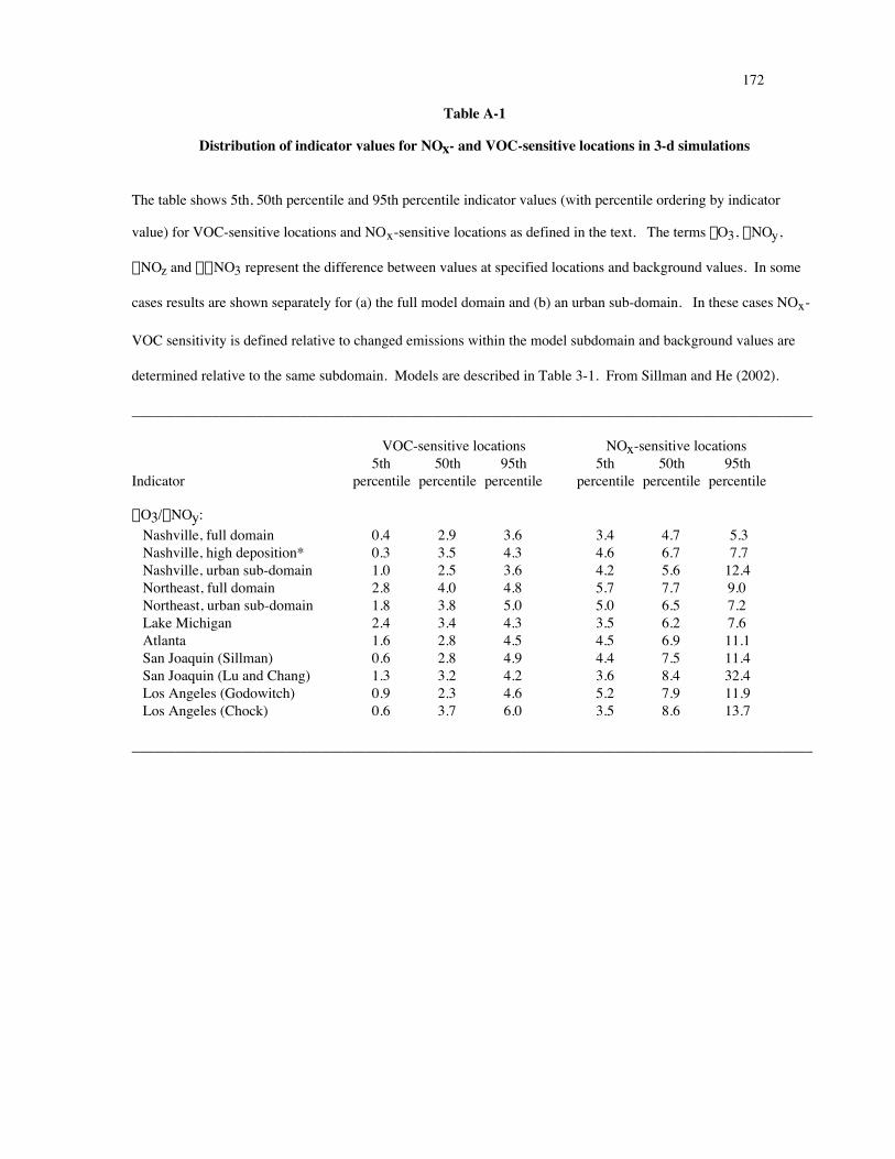
172

Table A-1

Distribution of indicator values for NOx- and VOC-sensitive locations in 3-d simulations

The table shows 5th, 50th percentile and 95th percentile indicator values (with percentile ordering by indicator

value) for VOC-sensitive locations and NOx-sensitive locations as defined in the text. The terms DO3, DNOy,

DNOz and DHNO3 represent the difference between values at specified locations and background values. In some

cases results are shown separately for (a) the full model domain and (b) an urban sub-domain. In these cases NOx-

VOC sensitivity is defined relative to changed emissions within the model subdomain and background values are

determined relative to the same subdomain. Models are described in Table 3-1. From Sillman and He (2002).

_____________________________________________________________________________________________

VOC-sensitive locations NOx-sensitive locations5th 50th 95th 5th 50th 95th

Indicator percentile percentile percentile percentile percentile percentile

DO3/DNOy: Nashville, full domain 0.4 2.9 3.6 3.4 4.7 5.3 Nashville, high deposition* 0.3 3.5 4.3 4.6 6.7 7.7 Nashville, urban sub-domain 1.0 2.5 3.6 4.2 5.6 12.4 Northeast, full domain 2.8 4.0 4.8 5.7 7.7 9.0 Northeast, urban sub-domain 1.8 3.8 5.0 5.0 6.5 7.2 Lake Michigan 2.4 3.4 4.3 3.5 6.2 7.6 Atlanta 1.6 2.8 4.5 4.5 6.9 11.1 San Joaquin (Sillman) 0.6 2.8 4.9 4.4 7.5 11.4 San Joaquin (Lu and Chang) 1.3 3.2 4.2 3.6 8.4 32.4 Los Angeles (Godowitch) 0.9 2.3 4.6 5.2 7.9 11.9 Los Angeles (Chock) 0.6 3.7 6.0 3.5 8.6 13.7

_____________________________________________________________________________________________

173

Table A-1 (continued)

_____________________________________________________________________________________________



DO3/DNOz: Nashville, full domain 1.2 3.6 5.0 3.8 5.3 6.1 Nashville, high deposition* 1.6 4.8 6.6 5.3 8.1 9.1 Nashville, urban sub-domain 1.9 4.0 5.0 5.1 7.1 15.4 Northeast, full domain 4.7 5.0 5.6 6.7 8.5 9.9 Northeast, urban sub-domain 2.8 4.4 5.4 5.7 7.4 8.3 Lake Michigan 3.0 4.0 5.2 5.7 7.3 8.5 Atlanta 3.6 4.5 5.9 6.1 9.2 14.6 San Joaquin (Sillman) 2.4 6.1 8.1 6.0 9.9 15.2 San Joaquin (Lu and Chang) 3.5 6.4 6.6 5.0 11.6 31.4 Los Angeles (Godowitch) 3.0 4.5 6.3 6.2 9.0 15.6 Los Angeles (Chock) 4.2 6.7 10.0 8.3 10.9 16.6

DO3/DHNO3: Nashville, full domain 1.4 4.2 6.5 4.6 6.7 8.2 Nashville, high deposition* 1.8 5.9 9.4 7.1 11.5 14.1 Nashville, urban sub-domain 2.2 5.1 7.9 8.0 12.8 40.3 Northeast, full domain 7.3 8.4 10.7 11.0 15.6 23.9 Northeast, urban sub-domain 4.9 8.4 11.4 13.1 27.3 235.7 Lake Michigan 3.6 4.8 7.6 8.8 12.5 18.2 Atlanta 4.1 5.3 7.3 7.3 13.1 20.5 San Joaquin (Sillman) 2.7 7.4 11.0 9.4 14.7 29.6 Los Angeles (Godowitch) 3.5 5.5 8.9 9.1 14.6 31.2 Los Angeles (Chock) 6.2 10.1 25.3 13.1 18.3 42.4

O3/NOy: Nashville 2.2 3.6 5.6 7.1 10.8 13. Nashville, high dep.* 2.6 5.3 7.2 8.7 13.9 17. Northeast corridor 5.0 5.4 6.5 8.2 12.7 18. Lake Michigan 3.5 5.2 6.6 7.2 11.7 16. Atlanta 3.6 5.1 7.2 8.1 14.3 27. Los Angeles (Godowitch) 1.4 3.2 6.0 7.2 10.4 20. Los Angeles (Chock) 1.0 5.4 9.1 5.9 18. 24. San Joaquin (Sillman) 3.0 7.3 11.6 15. 26. 56. San Joaquin (Chang) 5.4 7.7 12.3 12.5 22. 52.

_____________________________________________________________________________________________

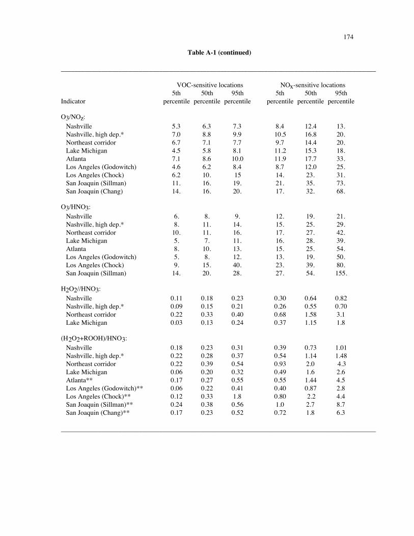
174

Table A-1 (continued)

_____________________________________________________________________________________________



O3/NOz: Nashville 5.3 6.3 7.3 8.4 12.4 13. Nashville, high dep.* 7.0 8.8 9.9 10.5 16.8 20. Northeast corridor 6.7 7.1 7.7 9.7 14.4 20. Lake Michigan 4.5 5.8 8.1 11.2 15.3 18. Atlanta 7.1 8.6 10.0 11.9 17.7 33. Los Angeles (Godowitch) 4.6 6.2 8.4 8.7 12.0 25. Los Angeles (Chock) 6.2 10. 15 14. 23. 31. San Joaquin (Sillman) 11. 16. 19. 21. 35. 73. San Joaquin (Chang) 14. 16. 20. 17. 32. 68.

O3/HNO3: Nashville 6. 8. 9. 12. 19. 21. Nashville, high dep.* 8. 11. 14. 15. 25. 29. Northeast corridor 10. 11. 16. 17. 27. 42. Lake Michigan 5. 7. 11. 16. 28. 39. Atlanta 8. 10. 13. 15. 25. 54. Los Angeles (Godowitch) 5. 8. 12. 13. 19. 50. Los Angeles (Chock) 9. 15. 40. 23. 39. 80. San Joaquin (Sillman) 14. 20. 28. 27. 54. 155.

H2O2//HNO3: Nashville 0.11 0.18 0.23 0.30 0.64 0.82 Nashville, high dep.* 0.09 0.15 0.21 0.26 0.55 0.70 Northeast corridor 0.22 0.33 0.40 0.68 1.58 3.1 Lake Michigan 0.03 0.13 0.24 0.37 1.15 1.8

(H2O2+ROOH)/HNO3: Nashville 0.18 0.23 0.31 0.39 0.73 1.01 Nashville, high dep.* 0.22 0.28 0.37 0.54 1.14 1.48 Northeast corridor 0.22 0.39 0.54 0.93 2.0 4.3 Lake Michigan 0.06 0.20 0.32 0.49 1.6 2.6 Atlanta** 0.17 0.27 0.55 0.55 1.44 4.5 Los Angeles (Godowitch)** 0.06 0.22 0.41 0.40 0.87 2.8 Los Angeles (Chock)** 0.12 0.33 1.8 0.80 2.2 4.4 San Joaquin (Sillman)** 0.24 0.38 0.56 1.0 2.7 8.7 San Joaquin (Chang)** 0.17 0.23 0.52 0.72 1.8 6.3

_____________________________________________________________________________________________

175

Table A-1 (concluded)

_____________________________________________________________________________________________



H2O2//NOz: Nashville 0.12 0.15 0.19 0.21 0.41 0.45 Nashville, high dep.* 0.10 0.13 0.17 0.18 0.37 0.41 Northeast corridor 0.14 0.20 0.21 0.36 0.80 1.4 Lake Michigan 0.03 0.10 0.19 0.27 0.60 0.87

(H2O2+ROOH)/NOz: Nashville 0.13 0.20 0.27 0.29 0.59 0.85 Nashville, high dep.* 0.15 0.22 0.30 0.35 0.79 1.08 Northeast corridor 0.14 0.24 0.28 0.49 1.10 1.91 Lake Michigan 0.05 0.15 0.26 0.35 0.81 1.22 Atlanta** 0.14 0.23 0.44 0.42 1.04 2.8 Los Angeles (Godowitch)** 0.05 0.17 0.33 0.26 0.55 1.4

H2O2/NOy: Nashville 0.05 0.09 0.12 0.17 0.36 0.42 Nashville, high dep.* 0.04 0.07 0.10 0.14 0.32 0.40 Northeast corridor 0.11 0.14 0.17 0.30 0.68 1.3 Lake Michigan 0.02 0.09 0.16 0.22 0.43 0.78

(H2O2+ROOH)/NOy: Nashville 0.08 0.12 0.18 0.24 0.52 0.98 Nashville, high dep.* 0.08 0.12 0.17 0.28 0.68 1.15 Northeast corridor 0.11 0.19 0.22 0.38 0.9 1.72 Lake Michigan 0.04 0.12 0.25 0.28 0.58 1.09 Atlanta** 0.10 0.12 0.19 0.29 0.83 2.2 Los Angeles (Godowitch)** 0.02 0.08 0.19 0.22 0.47 1.2

_____________________________________________________________________________________________

* The Nashville high deposition scenario has dry deposition rates of 5 cm2 s-1 for H2O2 and HNO3, as opposed to2.5 cm2 s-1 in the standard scenario.

** In models with CB-4 chemistry, "H2O2" is interpreted as a surrogate for the sum of H2O2 and organic peroxides.

Documents

DRAFT - University of Michigan