Embed Size (px)
Citation preview
Srinivas R. Chakravarthy MATH-602: LECTURE 11 (WINTER 2000) 1
MATH602: APPLIED STATISTICS Winter 2000
Dr. Srinivas R. Chakravarthy
Department of Industrial and Manufacturing Engineering & Business
Kettering University (Formerly GMI Engineering & Management Institute)
Flint, MI 48504-4898 Phone: (810) 762-7906; FAX: (810) 762-9944
E-mail: [email protected] Homepage: http://www.kettering.edu/~schakrav

Srinivas R. Chakravarthy MATH-602: LECTURE 11 (WINTER 2000) 2
TAGUCHI APPROACH TO QUALITY
• So far we saw the classical DOE and some specific
designs, and their analysis. • Dr. Genichi Taguchi of Japan has incorporated a number
of quality engineering methods that use DOE with an idea to design high-quality systems at reduced cost.
• These methods provide an efficient and systematic approach to optimize designs for performance, quality and cost.
• These methods emphasize designing quality into the products and processes, compared to the standard method of inspection for quality.

Srinivas R. Chakravarthy MATH-602: LECTURE 11 (WINTER 2000) 3
• These have been very effective in improving quality of Japanese products, and hence got popular in western industries.
• Although there is some controversy about Taguchi’s methods in terms of the philosophical and technical aspects, here we will briefly illustrate the basic ideas and the usefulness of these designs in practice.
• Note that until before Taguchi’s methods were introduced, traditional designs were used only to assess effect on averages.
• However, Taguchi made experimenters aware of the value in using the designs to assess the impact of factors on the variability of the response variable.

Srinivas R. Chakravarthy MATH-602: LECTURE 11 (WINTER 2000) 4
• In practice, one usually deals with many factors to study a response variable.
• This leads to the study of many test combinations in the case of a full study.
• A standard method of reducing the number of test runs is to use fractional factorial designs (recall this from earlier lecture on DOE).
• Taguchi constructed a special set of general designs that consist of orthogonal arrays.
• These determine the least number of test runs for a given number of factors to be studied.

Srinivas R. Chakravarthy MATH-602: LECTURE 11 (WINTER 2000) 5
• Before we see these, we will review some basic concepts needed for better understanding of these designs.
• One of the misconceptions in the quality of a product is that “as long as the data points fall within a specified interval there is no need for any action”.
• For example, take the case study conducted by Sony Corporation. The study was focused to determine a cause for the difference in customer preference.
• Sony manufactures color TV’s in Japan as well as in USA. The study included TV’s produced in these two countries, intended for market in USA.

Srinivas R. Chakravarthy MATH-602: LECTURE 11 (WINTER 2000) 6
• Hence, they have identical design and system tolerances. American consumers consistently preferred the color characteristics of the TV sets produced in Japan.
• Even though the plants in Japan as well as USA shipped only those TVs that are within specifications, the TV’s produced in USA have a more flat curve indicating more variability in the color density.
• This clearly indicates that “meeting specifications” is not sufficient for the quality of the product in many cases.
• The quality of a product goes beyond this and the bottom line is to meet the target as much as possible not only to increase the quality but also to minimize the loss to the society.

Srinivas R. Chakravarthy MATH-602: LECTURE 11 (WINTER 2000) 7
• Note that the cost is measured not only in terms of manufacturers (through reduction in the sales of the units, warranty costs, replacement costs) but also the consumers have to pay (through repairs, replacements, increase in the price of the units set by the manufacturer to off-set any loss in the manufacturing stage).
• Usually this cost is referred to as the loss to the society. Thus, a poorly designed product causes the society to incur losses from the initial stage through the final product usage stage.
Srinivas R. Chakravarthy MATH-602: LECTURE 11 (WINTER 2000) 8
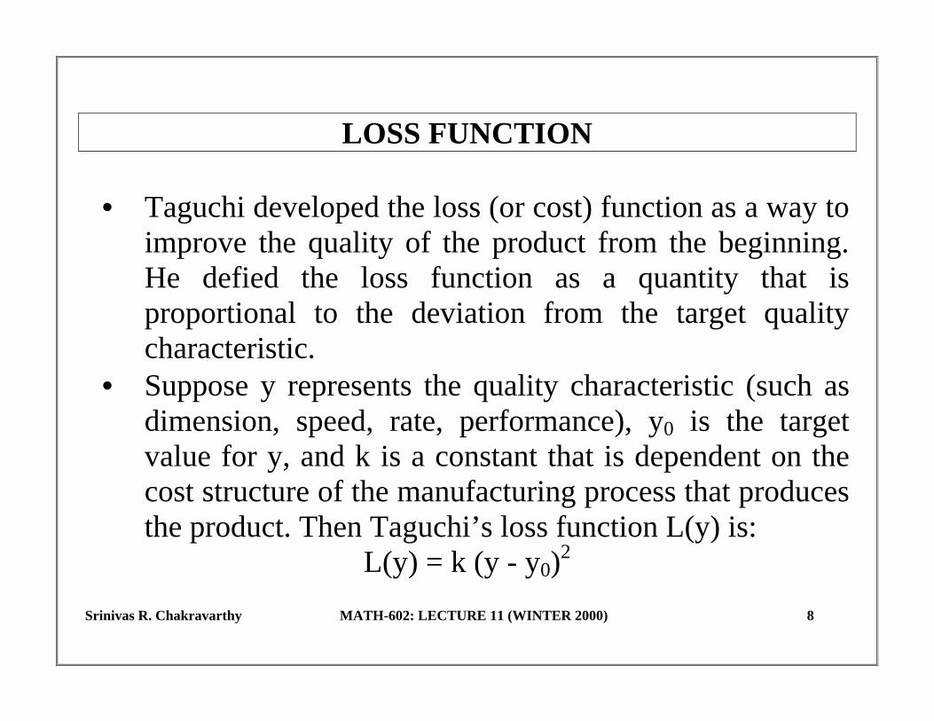
LOSS FUNCTION • Taguchi developed the loss (or cost) function as a way to
improve the quality of the product from the beginning. He defied the loss function as a quantity that is proportional to the deviation from the target quality characteristic.
• Suppose y represents the quality characteristic (such as dimension, speed, rate, performance), y0 is the target value for y, and k is a constant that is dependent on the cost structure of the manufacturing process that produces the product. Then Taguchi’s loss function L(y) is:
L(y) = k (y - y0)2

Srinivas R. Chakravarthy MATH-602: LECTURE 11 (WINTER 2000) 9
• Note that this function possesses the following
properties: (a) the loss must be zero when target is attained; (b) the magnitude of the loss increases rapidly as y
deviates farther away from the target value; (c) the loss function is a continuous function of the
deviation.

Srinivas R. Chakravarthy MATH-602: LECTURE 11 (WINTER 2000) 10
QUALITY CHARACTERISTICS
• As we saw earlier, the quality of a product can be
measured in many ways depending on the intent of the product.
• For example, o the quality of a light bulb may be measure in terms of
the number of hours of life; o the bonding strength is the amount of pressure needed
before the bonding units can be separated; o the amount of SO2 emitted by using a particular type
of filter in the release chamber;

Srinivas R. Chakravarthy MATH-602: LECTURE 11 (WINTER 2000) 11
o the voltage of level of a resistor. No matter how the quality of a product is defined, the measure will fall under one of the following three characteristics:
(A) the smaller the better (B) the larger the better (C) the nominal is best
• Verify that
o examples 1 and 2 fall under B; o example 3 falls under A and o example 4 falls under C.

Srinivas R. Chakravarthy MATH-602: LECTURE 11 (WINTER 2000) 12
ORTHOGONAL ARRAYS • Earlier we saw how factorial designs (FD) and fractional
factorial designs (FFD) were used in practice. • FFD is a means to reduce the number of runs needed
when the number of factors is large. In choosing a FFD for a study, certain treatment conditions are chosen in order to maintain the orthogonality among the various main effects and interaction effects.
• Orthogonal arrays were first recorded sometime in 1897 by French Mathematician J. Hadamard; but the utility of these were not explored until World War II by British Statisticians: Plackett and Burman.

Srinivas R. Chakravarthy MATH-602: LECTURE 11 (WINTER 2000) 13
• Taguchi has developed a family of FFD=s that can be utilized in various situations.
• The associated design matrices are labeled as L* where * is a selected positive integer.
• L stands for Latin square design, as these designs are simply a form of well known designs such as Plackett-Burman, FFD or Latin square designs.
• However, the combination of the loss function and the robust designs to find optimal settings is one of the strongest aspects of Taguchi=s method.
• The construction and the use of Latin squares orthogonal
arrays date back to the period of World War II mainly in

Srinivas R. Chakravarthy MATH-602: LECTURE 11 (WINTER 2000) 14
the context of agricultural applications. Since then they have been used extensively in many applications.
• Taguchi constructed a new set of OA’s using the
orthogonal Latin squares in a unique way. • This construction along with a set of rules for choosing a
particular OA has simplified the task for many engineers and statisticians, who apply DOE in practice.
• Below we will illustrate the use of Taguchi’s OA by
taking L4 and L8 OA’s.

Srinivas R. Chakravarthy MATH-602: LECTURE 11 (WINTER 2000) 15
L4 ORTHOGONAL ARRAY Consider an L4 OA, which is given in Table 1 below.
Table 1: L4 Orthogonal Array Run Column number
1 2 3 1 2 3 4
-1 -1 -1 -1 1 1 1 -1 1 1 1 -1

Srinivas R. Chakravarthy MATH-602: LECTURE 11 (WINTER 2000) 16
• From the above table, we see that an L4 experiment consists of four rows and three columns.
• Each row corresponds to a particular run in the experiment and each column corresponds to the factors specified in the study.
• Each column contains 2 low levels and 2 high levels for the factor assigned to that column.
• We use -1 for low level and 1 for high level. • In the first run, for example, the three design variables
are set at their low level and in the second run, the first parameter is set at low level and the remaining two variables are set at high level, and so on.

Srinivas R. Chakravarthy MATH-602: LECTURE 11 (WINTER 2000) 17
L8 ORTHOGONAL ARRAY This OA, which is displayed in Table 2 below, is a common OA for two level factors.
Table 2: L8 Orthogonal Array Run Column number
1 2 3 4 5 6 7 1 2 3 4 5 6 7 8
-1 -1 -1 -1 -1 -1 -1 -1 -1 -1 1 1 1 1 -1 1 1 -1 -1 1 1 -1 1 1 1 -1 -1 -1 1 -1 1 -1 1 -1 1 1 -1 1 1 -1 1 -1 1 1 -1 -1 1 1 -1 1 1 -1 1 -1 -1 1

Srinivas R. Chakravarthy MATH-602: LECTURE 11 (WINTER 2000) 18
• Notice that this is a one-sixteenth FFD, which has only the 8 of the total possible 128 runs.
• The seven columns are used to assign up to 7 factors. If only three factors are of interest, then this will become a full factorial design.
• When all columns are assigned a factor, this is known as a saturated design.
• In general, a FFD is said to be saturated when the design only allows for the estimation of main effects.
• These designs are effective when used as part of screening process when there are a number of factors to be examined.

Srinivas R. Chakravarthy MATH-602: LECTURE 11 (WINTER 2000) 19
• There are two sets of Taguchi’s OA’s available for use in practice:
��one set deals with 2-level factors, which are denoted by L4, L8, L12, L16, L32;
��the second set deals with 3-level factors: L9, L18, and L27.

Srinivas R. Chakravarthy MATH-602: LECTURE 11 (WINTER 2000) 20
SELECTION OF AN OA • The selection of an OA depends on the number of factors
(as well as the number of levels for each factor) and interactions of factors to be studied.
• Once this is finalized then an appropriate OA can be
chosen for the study. • If the number of levels of all factors to be studied is two,
then one of the L4, L8, L12, L16, and L32 can be chosen; if the number of levels of all factors is 3, then one of the L9, L18, and L27 OA’s can be chosen.

Srinivas R. Chakravarthy MATH-602: LECTURE 11 (WINTER 2000) 21
• If some factors are at two levels and others are at three levels, the predominant one will dictate which OA to be selected.
• For example, if there are 4 factors at 2 levels and 7 factors are at 3 levels, then 3-level design can be chosen. Thus, we will only concentrate on all factors at 2-level case r all at 3 level here.
• Note that the total number of degrees of freedom with n trials is n-1.
• Thus when choosing an OA, we have to make sure that the number of degrees of freedom in our study doesn’t exceed the number of columns available in the OA.

Srinivas R. Chakravarthy MATH-602: LECTURE 11 (WINTER 2000) 22
• For example, if four factors (without any interaction) are to be studied, then we need to select an OA: Lr, such that r > 4. This implies that we need to select L8 or L12, L16, or L32 OA.
• Suppose interactions of some factors are also to be included in the study.
• In this case the selection of an OA is little more complex.
• For example, suppose four factors: A-D and two interactions: AB and CD are to be studied. In this case, even though there are only 6 effects are being studied leading to 6 degrees of freedom, an L8 OA will not be

Srinivas R. Chakravarthy MATH-602: LECTURE 11 (WINTER 2000) 23
sufficient. In fact choosing an L8 OA will only result in confounding the effects of AB and CD.
• Thus, selecting an OA is easily achieved once the number of degrees of freedom in the study is determined along with the number of levels of the factors.
• Usually one of the above mentioned OA’s is sufficient for most examples.
• However, if these tables are not adequate, then Taguchi has tabulated a total of 18 standard orthogonal arrays which can be found in many text books dealing with Taguchi methods (see some references at the end).

Srinivas R. Chakravarthy MATH-602: LECTURE 11 (WINTER 2000) 24
ASSIGNMENT OF FACTORS TO COLUMNS • As you would have seen there are several columns
available in an OA. • The question is how to assign the factors (and the
interactions of the factors, if any) to these columns? • They cannot be done arbitrarily as confounding of the
factors will result. • Taguchi devised a scheme to assign factors and
interactions using linear graphs and triangular tables.

Srinivas R. Chakravarthy MATH-602: LECTURE 11 (WINTER 2000) 25
• The purpose of linear graphs is to indicate which factors may be assigned to which columns and the purpose of the triangular tables is to identify appropriate columns to assign the interactions.
• Usually there will be more than one choice for the assignment. However, careful assignment is necessary to avoid any unnecessary confounding effects.
• Any unassigned columns will be used to estimate the error sum of squares.

Srinivas R. Chakravarthy MATH-602: LECTURE 11 (WINTER 2000) 26
Example 1: Consider an L4 OA. This one has 3 columns and so three factors or two factors and an interaction of these two factors can be assigned to these columns. For example, Factor A can be assigned to column 1 and Factor B can be assigned to column 2. The interaction AB is now assigned to column 3. Now this assignment resembles the design matrix corresponding to a 22 full factorial design except that the interaction effect is really -AB.[Why?]. However, if interaction term is negligible or if one is not interested in it, then another factor, say, Factor C can be assigned to column 3.
Srinivas R. Chakravarthy MATH-602: LECTURE 11 (WINTER 2000) 27
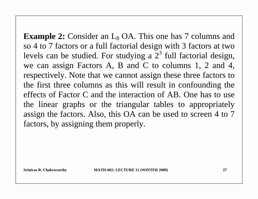
Example 2: Consider an L8 OA. This one has 7 columns and so 4 to 7 factors or a full factorial design with 3 factors at two levels can be studied. For studying a 23 full factorial design, we can assign Factors A, B and C to columns 1, 2 and 4, respectively. Note that we cannot assign these three factors to the first three columns as this will result in confounding the effects of Factor C and the interaction of AB. One has to use the linear graphs or the triangular tables to appropriately assign the factors. Also, this OA can be used to screen 4 to 7 factors, by assigning them properly.
Srinivas R. Chakravarthy MATH-602: LECTURE 11 (WINTER 2000) 28
• The following table summarizes the key observations for some commonly used Oas. The column headings are defined as:
(1): Number of levels for the factors; (2): Number of factors for a FFD; (3): Number of screening factors.
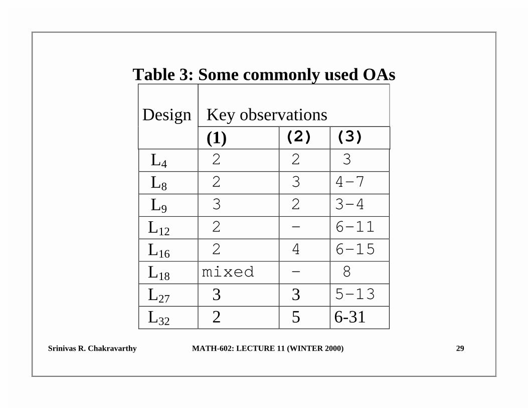
Srinivas R. Chakravarthy MATH-602: LECTURE 11 (WINTER 2000) 29
Table 3: Some commonly used OAs Key observations
Design
(1) (2) (3)
L4 2 2 3
L8 2 3 4-7
L9 3 2 3-4
L12 2 - 6-11
L16 2 4 6-15
L18 mixed - 8
L27 3 3 5-13
L32 2 5 6-31

Srinivas R. Chakravarthy MATH-602: LECTURE 11 (WINTER 2000) 30
SYSTEM, PARAMETER AND TOLERANCE DESIGNS • Earlier we saw how DOE is used to select the optimum
settings for each factor that will optimize the response variable.
• The factors that are studied for the design and that can be controlled are referred to as controlled factors or design parameters.
• There are other factors that affect the final product that are either difficult to control or cannot be controlled at all.
• These factors are referred to as noise factors.

Srinivas R. Chakravarthy MATH-602: LECTURE 11 (WINTER 2000) 31
• For example, the spring type, the way it is coiled, and where it is positioned, are some key factors in a suspension system in a car that can be controlled.
• However, the conditions of the road where the suspension systems will be subjected cannot be controlled. Thus the road condition is a noise factor.
• Variation in the noise factors during the manufacturing causes variation in the response variable.
• There could be many settings of the controlled factors at which the system can perform “better” on the average.
• Among these settings, there may be some at which the system may be insensitive to the noise factors.

Srinivas R. Chakravarthy MATH-602: LECTURE 11 (WINTER 2000) 32
• Taguchi recommended identifying the levels of design parameters that will minimize the impact of the noise factors on the product through experimentation.
• This way the control factors can be set at those levels to make the product more robust to noise factors.
• This is one of the biggest contributions of Taguchi to quality design.
• Thus, Taguchi looks at the design of a product as a three-phase problem:

Srinivas R. Chakravarthy MATH-602: LECTURE 11 (WINTER 2000) 33
(a) System design: New concepts, ideas, and methods are used to develop a new product. Applying existing scientific and engineering knowledge, a prototype design for a new product is developed. Also, here initial selection of parts, materials, etc are made and the main emphasis is to meet customer requirements at lower cost. (b) Parameter design: The goal here is to find the optimum settings for the controllable factors (also called parameters). This phase is crucial to achieve the uniformity of a product. (c) Tolerance design: This phase is done after the parameter design phase. Here the tolerances for the parameters are identified. This is very important in order to improve the quality of a product at a minimal cost and also stay on top of the competition.

Srinivas R. Chakravarthy MATH-602: LECTURE 11 (WINTER 2000) 34
INNER AND OUTER ARRAYS • Taguchi proposed a collection of techniques to identify
the settings for the controlled factors that will yield a robust performance.
• These include the selection of the DOE and the statistical analysis of the data.
• First select a DOE for the controlled factors. The design matrix for this is referred to as an inner array.
• Now select a DOE for the noise factors. The design matrix for this is referred to as an outer array.
• For each combination of factors in an inner array, run all combinations of the noise factors in the outer array.

Srinivas R. Chakravarthy MATH-602: LECTURE 11 (WINTER 2000) 35
• Taguchi classifies the parameter design problems into different categories (see the section on quality characteristic) and the effects are evaluated using the concept: signal-to-noise ratio.
SIGNAL-TO-NOISE RATIO
• Taguchi proposed a class of statistics, called signal-to-
noise ratios (S/N) to measure the effect of noise factors on performance characteristics.
• These S/N ratios take into account the amount of variability in the response variable as well as the closeness of average response to the target value.

Srinivas R. Chakravarthy MATH-602: LECTURE 11 (WINTER 2000) 36
• The commonly used ones correspond to the three quality characteristics mentioned above.
• Suppose that y1, . . . , yn are n observations on the response variable Y.
• Then S/N ratio for the three characteristics are defined as follows.
(A) The smaller the better: The “target” value for the response is zero (why?). Thus, for this
) /ny( 10 - = ratio S/N 2i
n
1 = i∑log

Srinivas R. Chakravarthy MATH-602: LECTURE 11 (WINTER 2000) 37
• The goal of the experiment here is to minimize the sum of the squared response values, which is equivalent to maximizing the S/N ratio.
(B) The larger the better: Here the goal is to maximize the response variable, which is equivalent to minimizing the reciprocal of the response value. Thus,
∑ ) y n / 1 ( 10 - = ratio S/N 2
i
n
1 = i
log
• The goal of the experiment here is to maximize the S/N
ratio.
Srinivas R. Chakravarthy MATH-602: LECTURE 11 (WINTER 2000) 38
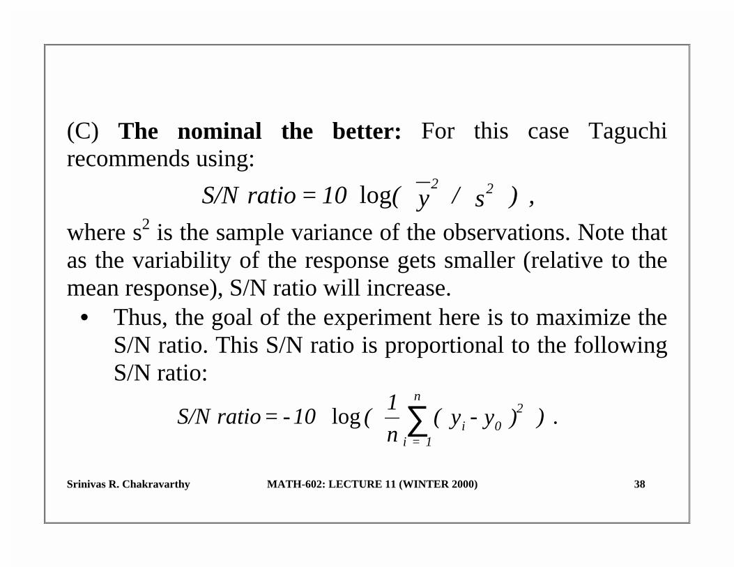
(C) The nominal the better: For this case Taguchi recommends using:
,) s / y ( 10 = ratio S/N 22log
where s2 is the sample variance of the observations. Note that as the variability of the response gets smaller (relative to the mean response), S/N ratio will increase. • Thus, the goal of the experiment here is to maximize the
S/N ratio. This S/N ratio is proportional to the following S/N ratio:
. ) ) y - y (n
1 ( 10- = ratio S/N 2
0i
n
1 = i∑log

Srinivas R. Chakravarthy MATH-602: LECTURE 11 (WINTER 2000) 39
ANALYSIS • The analysis of designs based on OAs is very similar to
the analysis of FFDs seen earlier.However, the earlier analysis concentrated on the effect of the controlled factors on the average response variable.
• But now there is some interest in the effect of the variation also. Using S/N ratio, the effect of variation is studied. G.E.P. Box (Signal-to-Noise ratios, performance criteria, and transformations, Technometrics1988) states that the use of S/N ratio concept is equivalent to an analysis of the logarithm of the data. (the assumption of the variance is proportional to the mean requires a logarithmic transformation to stabilize the condition.

Srinivas R. Chakravarthy MATH-602: LECTURE 11 (WINTER 2000) 40
Taguchi- Illustrative Example 1 The purpose of this example is to illustrate the use of S/N ratios as well as ln(s) method. The data for this is given in table 2 below. The solution will be discussed in the class.
Table 2 Run
A B C
y1 y2
y
s2
1 -1 -1 1 11 19 15 32 2 1 -1 -1 4 6 5 2 3 -1 1 -1 16 14 15 2 4 1 1 1 9 1 5 32

Srinivas R. Chakravarthy MATH-602: LECTURE 11 (WINTER 2000) 41
Taguchi - Illustrative Example 2 • An injection molding process engineer is interested in
identifying the factors that contribute to variability in part shrinkage as well as to determine the best settings for the factors that will minimize the shrinkage.
• Part shrinkage is measured as the amount of deviation from the desired part size. o Seven controlled factors: A-Cycle time; B-Mold
temperature; C-Holding pressure; D-Gate size; E-Cavity thickness; F-Holding time; G-Screw speed;
o 3 noise factors: H-Ambient temperature; I-Moisture content; J-Percent regrind;
were identified after a brain storming session.

Srinivas R. Chakravarthy MATH-602: LECTURE 11 (WINTER 2000) 42
Table 3: L8 Orthogonal Array for illustrative example 2 -1 1 1 -1 -1 1 -1 1 -1 -1 1 1
Run
A B C D E F G Y1 Y2 Y3 Y4
1 2 3 4 5 6 7 8
-1 -1 -1 -1 -1 -1 -1 -1 -1 -1 1 1 1 1 -1 1 1 -1 -1 1 1 -1 1 1 1 -1 -1 -1 1 -1 1 -1 1 -1 1 1 -1 1 1 -1 1 -1 1 1 -1 -1 1 1 -1 1 1 -1 1 -1 -1 1
2.6 2.7 2.8 2.8 0.8 3.0 0.8 3.2 3.6 1.0 3.3 0.9 2.5 2.4 2.5 2.3 3.5 3.6 3.5 3.5 2.6 4.7 3.6 1.5 4.5 2.4 2.7 5.1 2.4 2.5 2.3 2.4

Srinivas R. Chakravarthy MATH-602: LECTURE 11 (WINTER 2000) 43
References
[1] R. Roy (1990): A primer on the Taguchi method, Van Nostrand. [2] R.H. Lochner and J. E. Matar (1990). Designing for quality, ASQC Quality Press. [3] P.J. Ross (1988). Taguchi techniques for quality engineering, McGraw Hill. [4] S.R. Schimdt and R.G. Launsby (1994). Understanding industrial designed experiments, Air academy press.

Srinivas R. Chakravarthy MATH-602: LECTURE 11 (WINTER 2000) 44
THREE CASE STUDIES IN DOE Here we will see some selected case studies taken from the following sources. 1. R. Roy (1990): A primer on the Taguchi method, Van Nostrand. 2. R.H. Lochner and J. E. Matar (1990). Designing for quality, ASQC Quality Press. 3. S.R. Schmidt and R.G. Launsby (1994). Understanding industrial designed experiments, Air academy press. For full details refer to these books.

Srinivas R. Chakravarthy MATH-602: LECTURE 11 (WINTER 2000) 45
Case Study 1: [Engine Value-Train Noise Study] The objective of this study is to identify the factor(s) that influence the noise emitted by the value-train of a newly developed engine. The following six factors (all at 2 levels) were identified in a brainstorming session. Also, it was decided that interaction effects were less important than the main effects. The factors and the levels are given below. A: Value guide clearance (low/high); B: Upper guide length (smaller/larger); C: Value geometry (type1/type 2); D: Seat concentricity (quality 1/quality 2); E: Lower guide length (location 1/loc 2); F: Valve face runout (type 1/type 2). An L8 OA was used, in which factors A-F were assigned to columns 1 through 6 and column 7 is left unassigned. The data for this study is given in table 1 below.

Srinivas R. Chakravarthy MATH-602: LECTURE 11 (WINTER 2000) 46
Table 1: L8 Orthogonal Array for Case study 1
Run
A B C D E F *
y
1 2 3 4 5 6 7 8
-1 -1 -1 -1 -1 -1 -1 -1 -1 -1 1 1 1 1 -1 1 1 -1 -1 1 1 -1 1 1 1 1 -1 -1 1 -1 1 -1 1 -1 1 1 -1 1 1 -1 1 -1 1 1 -1 -1 1 1 -1 1 1 -1 1 -1 -1 1
45 34 56 45 46 34 39 43
Srinivas R. Chakravarthy MATH-602: LECTURE 11 (WINTER 2000) 47
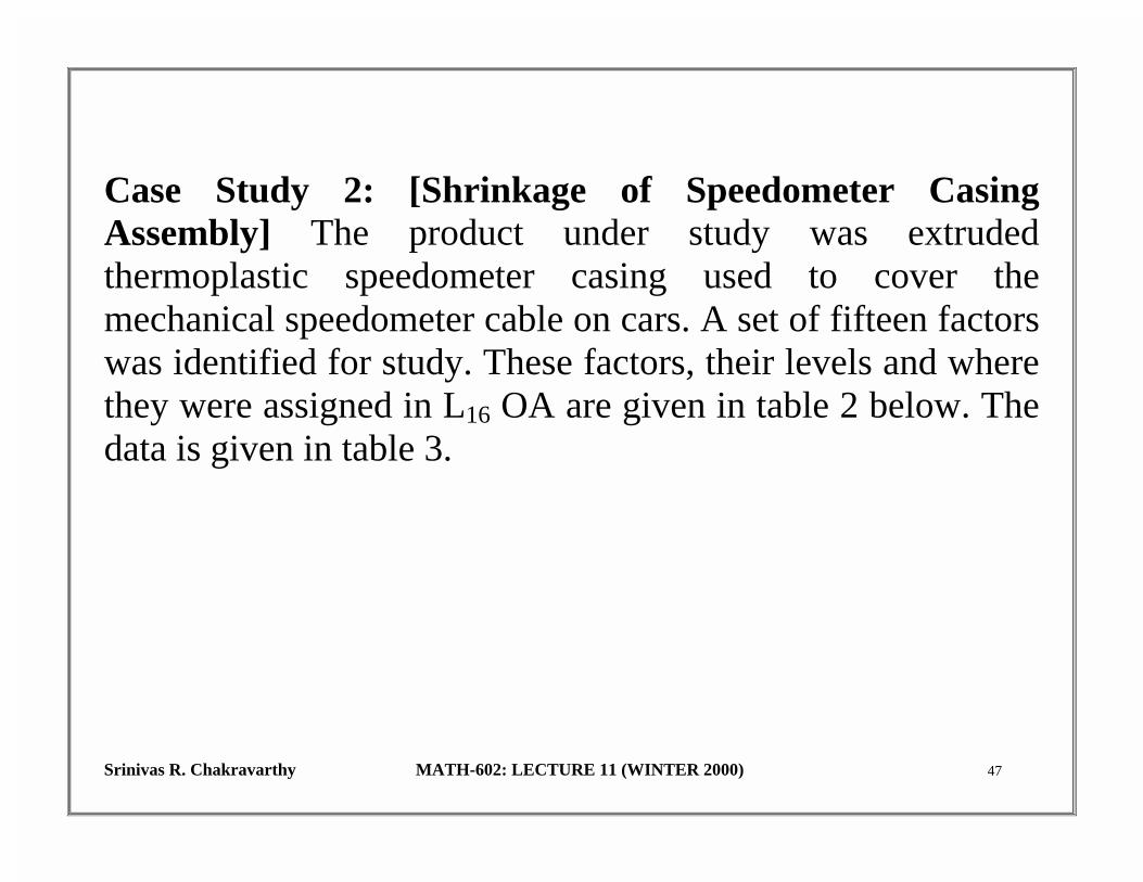
Case Study 2: [Shrinkage of Speedometer Casing Assembly] The product under study was extruded thermoplastic speedometer casing used to cover the mechanical speedometer cable on cars. A set of fifteen factors was identified for study. These factors, their levels and where they were assigned in L16 OA are given in table 2 below. The data is given in table 3.

Srinivas R. Chakravarthy MATH-602: LECTURE 11 (WINTER 2000) 48
Table 2: Factors, levels and column assignment Factor Level -1/+1 Column A: Liner O.D B: Liner die C: Liner line speed D: Liner tension E: Wire diameter F: Coating die type G: Screen pack H: Cooling method I: Line speed J: Liner material K: Wire braid type L: Liner temperature M: Braiding tension N: Coating material O: Melt temperature
Changed/existing Changed/existing 80%existing/existing More/existing existing/smaller Changed/existing denser/existing Changed/existing 70%existing/existing Changed/existing Changed/existing preheated/ambient Changed/existing Changed/existing Cooler/existing
1 2 3 4 11 12 13 14 15 5 6 7 8 9 10

Srinivas R. Chakravarthy MATH-602: LECTURE 11 (WINTER 2000) 49
Table 3: Data for Case study 2 Standard Order Observed values (4 replicates) 1 2 3 4 5 6 7 8 9 10 11 12 13 14 15 16
0.58 0.62 0.59 0.54 0.34 0.32 0.30 0.41 0.28 0.26 0.26 0.30 0.13 0.17 0.21 0.17 0.54 0.53 0.53 0.54 0.48 0.49 0.44 0.41 0.07 0.04 0.19 0.18 0.08 0.10 0.14 0.18 0.13 0.19 0.19 0.19 0.24 0.22 0.19 0.25 0.16 0.17 0.13 0.12 0.13 0.22 0.20 0.23 0.16 0.16 0.19 0.19 0.07 0.09 0.11 0.08 0.55 0.60 0.57 0.58 0.49 0.54 0.46 0.45

Srinivas R. Chakravarthy MATH-602: LECTURE 11 (WINTER 2000) 50
Case Study 3: [Optimization of an activated sludge reactor] This is an application of DOE in environmental engineering. The activated sludge process is a biological treatment system used at many wastewater treatment plants. Basically, the biological organisms (sludge) within the reactor are used to aerobically convert incoming waste into additional biomass or innocuous carbon dioxide and water. At the next stage liquid and solids are separated. The sludge is either waster or recycled back to the reactor to maintain an acceptable biomass population. Five key parameters are identified for the study: A-Reactor biomass concentration (3000/6000 mg/L); B-clarifier biomass concentration (8000/12000 mg/L); C-biological growth rate constant (0.040/0.075 d-1);D-fraction of food to biomass

Srinivas R. Chakravarthy MATH-602: LECTURE 11 (WINTER 2000) 51
(0.40/0.80 kg/kg); E-waste flow rate (785./940 m3). The response variable (y) is the biochemical oxygen demand, which is the amount of oxygen required to stabilize the decomposition matter in a water using aerobic biochemical action. Initially a two level design involving these five variables was proposed. Since 32 runs are needed for a full factorial design, a quarter factorial design (25-2) was conducted. The following table gives the aliasing structure as well as the data for the study.

Srinivas R. Chakravarthy MATH-602: LECTURE 11 (WINTER 2000) 52
Table 4: Data for Case study 3
Run
A B E C AE BE D AB ABE
y
1 2 3 4 5 6 7 8
1 1 1 1 1 1 1 1 1 -1 1 -1 -1 -1 1 -1 1 -1 1 -1 -1 1 -1 -1 -1 -1 1 1 -1 1 1 -1 -1 1 -1 -1 1 -1 -1 1 -1 1 -1 -1 1 1 -1 -1 1 -1 -1 -1 1 1 1 -1
775 354 1001 102 1371 87 496 195