Downlink Capacity of Distributed Antenna Systems in a ...cdn.intechweb.org/pdfs/12039.pdf · Downlink Capacity of Distributed Antenna ... In this chapter, without loss of generality,

8

Downlink Capacity of Distributed Antenna Systems in a Multi-Cell Environment

Wei Feng, Yunzhou Li, Shidong Zhou and Jing Wang State Key Laboratory on Microwave and Digital Communications

Tsinghua National Laboratory for Information Science and Technology Department of Electronic Engineering, Tsinghua University, Beijing 100084,

P. R. China

1. Introduction

The future wireless networks will provide data services at a high bit rate for a large number

of users. Distributed antenna system (DAS), as a promising technique, has attracted

worldwide research interests (Feng et al., 2010; 2009; Saleh et al., 1987; Ni & Li, 2004; Xiao et

al., 2003; Zhuang et al., 2003; Hasegawa et al., 2003; Choi & Andrews, 2007; Roh & Paulraj,

2002b;a). In DAS, the antenna elements are geographically separated from each other in the

coverage area, and the optical fibers are employed to transfer information and signaling

between the distributed antennas and the central processor where all signals are jointly

processed. Recent tudies have identified the advantages of AS n terms of increased system

capacity (Ni & Li, 004; Xiao et al., 2003; Zhuang et al., 2003; Hasegawa t al., 2003; Choi &

Andrews, 2007) and acro diversity (Roh & Paulraj, 2002b;a) as well as coverage

improvement (Saleh et al., 1987).

Since the demand for high bit rate data service will be dominant in the downlink, many

studies on DAS have focused on analyzing the system performance in the downlink. In a

single cell environment, the downlink capacity of a DAS was investigated in virtue of

traditional MIMO theory (Ni & Li, 2004; Xiao et al., 2003; Zhuang et al., 2003). However,

these studies did not consider per distributed antenna power constraint, which is a more

practical assumption than total transmit power constraint. Moreover, the advantage of a

DAS should be characterized in a multi-cell environment. (Hasegawa et al., 2003) addressed

the downlink performance of a code division multiple access (CDMA) DAS in a multi-cell

environment using computer simulations, but it did not provide theoretical analysis. A

recent work (Choi & Andrews, 2007) investigated the downlink capacity of a DAS with per

distributed antenna power constraint in a multi-cell environment and derived an analytical

expression. However, it was only applicable for single-antenna mobile terminals.

In this chapter, without loss of generality, the DAS with random antenna layout (Zhuang et

al., 2003) is investigated. We focus on characterizing the downlink capacity with the

generalized assumptions: (a1) per distributed antenna power constraint, (a2) generalized

mobile terminals equipped with multiple antennas, (a3) a multi-cell environment. Based on

system scale-up, we derive a quite good approximation of the ergodic downlink capacity by

adopting random matrix theory. We also propose an iterative method to calculate the

Source: Communications and Networking, Book edited by: Jun Peng, ISBN 978-953-307-114-5, pp. 434, September 2010, Sciyo, Croatia, downloaded from SCIYO.COM

www.intechopen.com

Communications and Networking

174

unknown parameter in the approximation. The approximation is illustrated to be quite

accurate and the iterative method is verified to be quite efficient by Monte Carlo

simulations.

The rest of this chapter is organized as follows. The system model is described in the next

section. Derivations of the ergodic downlink capacity are derived in Section 3. Simulation

results are shown in Section 4. Finally, conclusions are given in Section 5.

Notations: Lower case and upper case boldface symbols denote vectors and matrices,

respectively. (.)T and (.)H denote the transpose and the transpose conjugate, respectively.

CM×N represents the complex matrix space composed of all M × N matrices and CN denotes a

complex Gaussian distribution. E(.) and Var(.) represent the expectation operator and

variance operator, respectively. In is an identity matrix with the dimension equal to n. “⊗”

denotes the Kronecker product.

2. System model

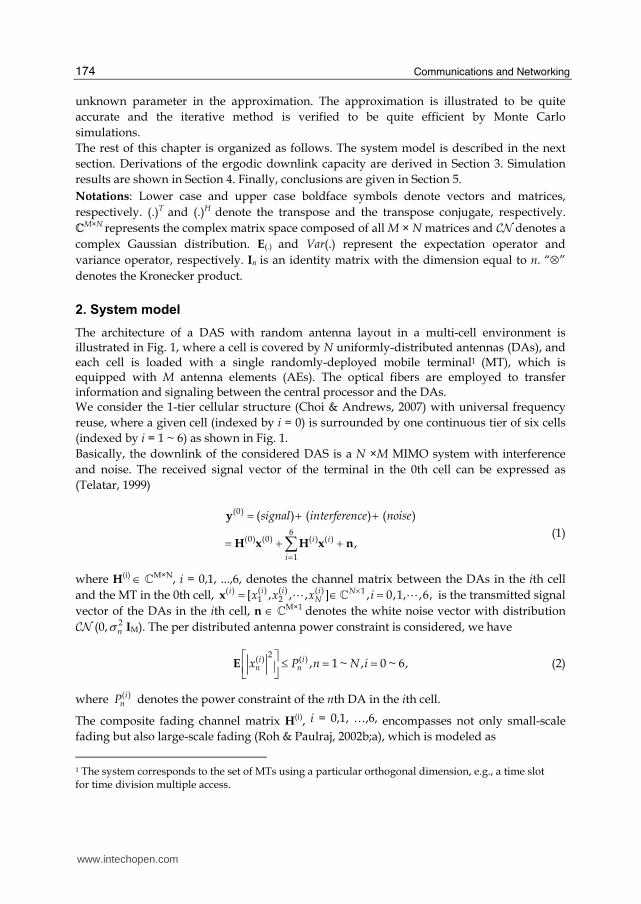
The architecture of a DAS with random antenna layout in a multi-cell environment is illustrated in Fig. 1, where a cell is covered by N uniformly-distributed antennas (DAs), and each cell is loaded with a single randomly-deployed mobile terminal1 (MT), which is equipped with M antenna elements (AEs). The optical fibers are employed to transfer information and signaling between the central processor and the DAs. We consider the 1-tier cellular structure (Choi & Andrews, 2007) with universal frequency

reuse, where a given cell (indexed by i = 0) is surrounded by one continuous tier of six cells

(indexed by i = 1 ~ 6) as shown in Fig. 1.

Basically, the downlink of the considered DAS is a N ×M MIMO system with interference

and noise. The received signal vector of the terminal in the 0th cell can be expressed as

(Telatar, 1999)

(0)

6(0) (0) ( ) ( )

1

( ) ( ) ( )

,i i

i

signal interference noise

=

= + += + +∑y

H x H x n (1)

where H(i) ∈ CM×N, i = 0,1, ...,6, denotes the channel matrix between the DAs in the ith cell

and the MT in the 0th cell, ( ) ( ) ( )( ) 11 2[ , , , ] , 0,1, ,6,i i ii N

Nx x x i×= ∈ =x A } A is the transmitted signal

vector of the DAs in the ith cell, n ∈ CM×1 denotes the white noise vector with distribution

CN (0, 2nσ IM). The per distributed antenna power constraint is considered, we have

2

( ) ( ) , 1 ~ , 0 ~ 6,i in nx P n N i

⎡ ⎤ ≤ = =⎢ ⎥⎣ ⎦E (2)

where ( )inP denotes the power constraint of the nth DA in the ith cell.

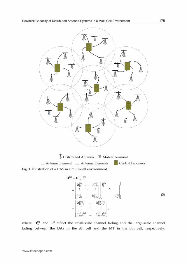
The composite fading channel matrix H(i), i = 0,1, …,6, encompasses not only small-scale

fading but also large-scale fading (Roh & Paulraj, 2002b;a), which is modeled as

1 The system corresponds to the set of MTs using a particular orthogonal dimension, e.g., a time slot for time division multiple access.

www.intechopen.com


175

Antenna Element Antenna Elements Central Processor

Distributed Antenna Mobile Terminal

Fig. 1. Illustration of a DAS in a multi-cell environment.

( ) ( ) ( )

( ) ( ) ( )11 1 1

( ) ( ) ( )1

( ) ( ) ( ) ( )11 1 1

( ) ( ) ( ) ( )1 1

,

i i iw

i i iN

i i iM MN N

i i i iN N

i i i iM MN N

h h l

h h l

h l h l

h l h l

=⎡ ⎤ ⎡ ⎤…⎢ ⎥ ⎢ ⎥= ⎢ ⎥ ⎢ ⎥⎢ ⎥ ⎢ ⎥…⎢ ⎥ ⎢ ⎥⎣ ⎦ ⎣ ⎦⎡ ⎤…⎢ ⎥= ⎢ ⎥⎢ ⎥…⎢ ⎥⎣ ⎦

H H L

B D B D

B D B

(3)

where ( )iwH and L(i) reflect the small-scale channel fading and the large-scale channel

fading between the DAs in the ith cell and the MT in the 0th cell, respectively.

www.intechopen.com


176

( ){ | 1,2, , ; 1,2, , ; 0,1, ,6}imnh m M n N i= = =A A A are independent and identically distributed

(i.i.d.) circularly symmetric complex Gaussian variables with zero mean and unit variance,

and ( ){ | 1,2, , ; 0,1, ,6}inl n N i= =A A can be modeled as

( ) ( ) ( ) , 1 ~ , 0 ~ 6,i i in n nl D S n N i

γ−⎡ ⎤= = =⎣ ⎦ (4)

where ( )inD and ( )i

nS are independent random variables representing the distance and the

shadowing between the MT in the 0th cell and the nth DA in the ith cell, respectively,

γ denotes the path loss exponent. ( )| 1,2, ... , ; 0,1,{ ... ,6}inS n N i= = are i.i.d. random

variables with probability density function (PDF)

2

2 2

1 (ln )( ) exp , 0,

2 2S

s s

sf s s

sπ λσ λ σ⎛ ⎞= − >⎜ ⎟⎜ ⎟⎝ ⎠ (5)

where σs is the shadowing standard deviation and ln1010

λ = .

Since the number of interfering source is sufficiently large and interfering sources are independent with each other, the interference plus noise is assumed to be a complex Gaussian random vector as follows:

6

( ) ( )

1

.i i

i

N=

= +∑H x n (6)

The variance of N is derived by the Central Limit Theorem as

6

( ) ( )2 2

1 1

( ) [ ]N

i in n n M

i n

Var l P σ= =

⎡ ⎤= +⎢ ⎥⎣ ⎦∑∑ IN (7)

2 .Mσ= I (8)

Therefore, (1) is rewritten as

(0) (0) (0) (0) .w= +y H L x N (9)

3. Downlink capacity characterization

3.1 Problem formulation

Since the small-scale fading always varies fast but the large-scale fading usually varies quite

slowly, we can regard L(0) as a static parameter in calculating the downlink capacity. Thus, if

the channel state information is only available at the receiver, the ergodic downlink capacity

is calculated by taking expectation over the small-scale fading (0)wH , which is expressed as

(Telatar, 1999)

(0 )(0) (0) (0) (0) (0)

2 2

1log det( ( ) ( ) )

w

HM w wC σ= +⎡ ⎤⎢ ⎥⎣ ⎦H

E I H L P H L , (10)

www.intechopen.com


177

where (0) (0) (0)(0)1 2diag{ , , , }NP P P P= A is the transmit power matrix of the DAs in the 0th cell.

Unfortunately, it is quite difficult to get a more compact expression of the ergodic downlink

capacity. Therefore, we propose the operation of “system scale-up” to study a simplified

method to calculate the capacity as accurately as possible.

3.2 System scale-up

The basic idea of system scale-up is illustrated in Fig. 2. Assuming the proportion between the initial system and the scaled-up system to be t (a positive integer), we can summarize the characteristics of system scale-up as follows:

• Each DA with a single AE is scaled to a DA cluster with t AEs.

• The number of AEs equipped on the MT is increased from M to Mt.

• The system topology is not changed.

• The variance of N is not changed.

• The large-scale channel fading is changed from L(i) to L(i)t, we have

( ) ( ) .i t it= ⊗L L I (11)

The small-scale fading is changed from ( )i M NwH ×∈} to ( )i t Mt Nt

wH ×∈} , 0,1, ,6i = A , let

( ) , 1 , 1 , 0,1, ,6i t t tmn m M n N i×∈ ≤ ≤ ≤ ≤ =H } A , we have

( ) ( )11 1

( )

( ) ( )11

, 0,1, ,6.

i iN

i tw

i iMN

H i

⎡ ⎤…⎢ ⎥= =⎢ ⎥⎢ ⎥…⎢ ⎥⎣ ⎦

H H

H H

B D B A (12)

( )i twH is also a matrix with i.i.d. zero-mean unit-variance circularly symmetric complex

Gaussian entries, which is the same as ( )iwH . • The total power consumption is not changed. In detail, the transmit power of each DA

in the initial system will be equally shared by the t AEs within a DA cluster in the scaled-up system. We can express the new transmit power matrix as

(0) (0) (0)(0)1 2

1diag{ , ,... ., }t tNP P P P

t= ⊗ I (13)

It is well known that the channel capacity of a MIMO system can be well approximated by a linear function of the minimum number of transmit and receive antennas (Telatar, 1999) as follows:

( , ) ,min a b A≈ ×} (14)

where C is the capacity of a MIMO channel with a transmit antennas and b receive antennas,

A is a corresponding fixed parameter determined by the total transmit power constraint. If

the number of transmit antennas and receive antennas increase from a to ta, from b to tb,

respectively, the channel capacity is derived as

ˆ ( , ) .min ta tb A t≈ × ≈} } (15)

www.intechopen.com


178

Fig. 2. Illustration of system scale-up.

www.intechopen.com


179

Since the considered DAS is a special MIMO system, we directly hold that the system capacity scales linearly in the process of system scale-up, which can be partial testified by the following Theorem. Theorem 1:

If the proportion between the initial system and the scaled-up system is t, an upper bound for the downlink capacity of the scaled-up system can be expressed as

(0) (0)2

2 21

( )log 1 .

Nupper n nt

n

l PC t M σ=

⎛ ⎞= × +⎜ ⎟⎜ ⎟⎝ ⎠∑ (16)

Proof: Based on (10), the capacity of the scaled-up system can be derived as

(0 )(0) (0) (0) (0) (0)

2 2

1log det( ( ) ( ) ) ,t

w

t t t t Ht Mt w t wC σ

⎡ ⎤= +⎢ ⎥⎣ ⎦HE I H L P H L (17)

According to Hadamard Inequation, we have

(0 )(0) (0) (0) (0) (0)

2 2 [ ]1

1log (1 ( ) ( ) ),t

w

Mtt t t t H

t w t wjj

j

C σ=⎡ ⎤≤ + ⎣ ⎦∑H

E H L P H L (18)

Directly put E inside log2, according to Jenson Inequation, we have

(0) (0)(0) (0) (0) (0) (0)

2 2 [ ]1

1log (1 ( ) ( ) ),t t

w w

Mtt t t t H

t w t wjj

j

C σ=⎡ ⎤≤ + ⎣ ⎦∑H H

E E H L P H L (19)

Then, from (11), (12) and (13), we can further derive

(0) (0)2

2 21

( )log 1 .

Nn n

tn

l PC t M σ=

⎛ ⎞≤ × +⎜ ⎟⎜ ⎟⎝ ⎠∑ (20)

Thus,

(0) (0)2

2 21

( )log 1 .

Nupper n nt

n

l PC t M σ=

⎛ ⎞= × +⎜ ⎟⎜ ⎟⎝ ⎠∑ (21)

■ Let

(0) (0)2

0 2 21

( )log 1 .

Nn n

n

l PC M σ=

⎛ ⎞= +⎜ ⎟⎜ ⎟⎝ ⎠∑ (22)

From Theorem 1, we have

0 .uppertC t C= × (23)

It is observed that the upper bound of the system capacity scales linearly in the process of system scale-up.

www.intechopen.com


180

3.3 Calculation of the downlink capacity

Based on the foregoing argument, we derive an approximation of the downlink ergodic capacity as

(0)(0) (0) (0)

2 2

1 1log det ,t

w

HMt t t tC

t σ⎧ ⎫⎡ ⎤≈ +⎨ ⎬⎢ ⎥⎣ ⎦⎩ ⎭H

E I H P H (24)

where (0)tH is the channel matrix of the scaled-up system

(0) (0) (0) (0)1 11 1

(0)

(0) (0) (0) (0)1 1

.N N

t

M N MN

l l

l l

⎡ ⎤…⎢ ⎥= ⎢ ⎥⎢ ⎥…⎢ ⎥⎣ ⎦

H H

H

H H

B D B (25)

We rewrite (24) as

(0 ) 2 2

1 1log det ,t

w

HMtC

t σ⎧ ⎫⎡ ⎤≈ +⎨ ⎬⎢ ⎥⎣ ⎦⎩ ⎭H

E I HH (26)

where Mt Nt×∈}H and

(0)(0)(0) (0) (0)11 11 1

(0)(0)(0) (0) (0) (0)11 1

.

NN N

NM N MN

PPl l

t t

H

PPl l

t t

⎡ ⎤⎢ ⎥…⎢ ⎥⎢ ⎥= ⎢ ⎥⎢ ⎥⎢ ⎥…⎢ ⎥⎣ ⎦

H H

H H

B D B (27)

Theorem 2:

The ergodic downlink capacity described in (10) can be accurately approximated as

(0) (0)2 1 12 2 22

1

1log (1 [ ] ) log ( ) log 1 ,

N

n nn

C C l P W M M W M e Wσ − −=

⎡ ⎤≈ = + + − −⎣ ⎦∑ (28)

where W is the solution of the following equation

(0) (0)2

(0) (0)2 2 11

[ ]1 .

[ ]

Nn n

n n n

l PW

l P W Mσ −== + +∑ (29)

Proof:

Let : [0, ) [0, )tv M N× → { be the variance profile function of matrix H, which is given by

11( , ) ( ( , )), [ , ); [ , ),t j ji i

v x y t Var i j x yt t t t

−−= ⋅ ∈ ∈H

where H(i, j) is the entry of matrix H with index (i, j). We can further find that as t → ∞,

vt(x,y) converges uniformly to a limiting bounded function v(x,y), which is given by

www.intechopen.com


181

(0) (0)2( , ) [ ] , [0, ); 1, ).} [n nv x y l P x M y n n= ∈ ∈ − (30)

Therefore, the constraints of Theorem 2.53 in (Tulino & Verdu, 2004) are satisfied, we can

derive the Shannon transform (Tulino & Verdu, 2004) of the asymptotic spectrum of HHH as

(0 ) 2

1( ) lim [log det( )]H t

w

H

tν ν

t→∞= +H

E IHHV HH (31)

2

2

, 2

[log (1 [ ( , ) ( , ) )])]

[log (1 [ ( , ) ( , ) )])]

[ ( , ) ( , ) ( , )]log ,

H

H

H H

E ν v νν v ν

ν v ν ν e

= + Γ+ + Υ− Γ Υ

Y X

X Y

X Y

E X Y X Y

E E X Y Y X

E X Y X Y

HH

HH

HH HH

∣

∣

with (.,.)HΓHH and (.,.)HΥHH satisfying the following equations

1

( , ) ,1 [ ( , ) ( , )]

H

H

x νν v x ν

Γ = + ΥYE Y YHHHH

(32)

1

Y ( , ) ,1 [ ( , ) ( , )]

H

H

y νν v y ν

= + ΓXE X XHHHH

(33)

where X and Y represent independent random variables, which are uniform on [0,M) and

[0,N), respectively, ν is a parameter in Shannon transform. Given ν , based on (30), we

can observe that ( , )H x νΓHH is constant on x ∈ [0,M) and ( , )H y νΥHH is constant on

y ∈ [n — 1,n). Thus, we define

1[0, )( , )| ,H x Mx ν W −∈Γ =HH (34)

1[ 1, )( , )| .H y n n ny ν U−∈ − =YHH (35)

From (32) and (33), we have

(0) (0)2 1

1

1 [ ] ,N

n n nn

W ν l P U−=

= + ∑ (36)

(0) (0)2 11 [ ] , 1 .n n nU ν l P W M n N−= + ≤ ≤ (37)

Assuming 21ν σ= , we can further derive

(0) (0)2 1 12 2 22 2

1

1 1( ) log (1 [ ] ) log ( ) log 1 .H

N

n nn

C l P W M M W M e Wσ σ − −=

⎡ ⎤≈ = + + − −⎣ ⎦∑HHV (38)

Moreover, from (36) and (37), W can be calculated by solving the following equation

(0) (0)2

(0) (0)2 2 11

[ ]1 .

[ ]

Nn n

n n n

l PW

l P W Mσ −== + +∑ (39)

■

www.intechopen.com


182

The unknown parameter W in Theorem 2 can be easily derived via an iterative method as presented in Table 1. The efficiency of the iterative algorithm will be demonstrated in Section 4.

0 6

(0) (0)2

(0) (0)2 2 1 11

21

1; 1.0 10 .

:

[ ] 1

[ ] ( )

.

:

.

Nl n n

ln n n

l l

Initializatio

W

Loopstep

l PW

l P W M

until W W

n

end

σ

−

− −=−

= = ×

= + +⎡ ⎤Δ = − <⎣ ⎦

∑ε

ε

Table 1. The iterative method to calculate W.

4. Simulation results

In this section, Monte Carlo simulations are used to verify the validity of our analysis. The

radius of a cell is assumed to be 1000m. The path loss exponent is set to be 4, the shadowing

standard deviation is set to be 4 according to field measurement for microcell environment

(Goldsmith & Greenstein, 1993), and the noise power 2nσ is set to be -107dBm. The per

distributed antenna power constraint takes value from -30dBm to 30dBm. Without loss of generality, four different simulation setups are considered as follows:

• Case 1: N = M = 4, with randomly-selected system topology as shown in Fig. 3-A;

• Case 2: N = M = 4, with randomly-selected system topology as shown in Fig. 3-B;

• Case 3: N = M = 8, with randomly-selected system topology as shown in Fig. 3-C;

• Case 4: N = M = 8, with randomly-selected system topology as shown in Fig. 3-D; Both analysis and simulation results of the ergodic downlink capacity for the four cases are presented in Fig. 4. It is observed that the two kinds of results are quite accordant with each other, which implies the high accuracy of the approximation in Theorem 2.

The total error covariance (Δ in Table 1) of the iterative method to calculate W is illustrated

in Fig. 5. We can observe that 40 iteration steps are enough to make Δ be less than 1.0 × 10−6. In summary, we can conclude that the approximation is accurate and the iterative method is efficient.

5. Conclusions

In this chapter, the problem of characterizing the downlink capacity of a DAS with random antenna layout is addressed with the generalized assumptions: (a1) per distributed antenna power constraint, (a2) generalized mobile terminals equipped with multiple antennas, (a3) a multi-cell environment. Based on system scale-up, we derive a good approximation of the ergodic downlink capacity by adopting random matrix theory. We also propose an iterative method to calculate the unknown parameter in the approximation. The approximation is illustrated to be quite accurate and the iterative method is verified to be quite efficient by Monte Carlo simulations.

www.intechopen.com


183

Mobile TerminalDistributed Antenna

A B

C D

Fig. 3. Randomly-selected system topologies for simulations.

www.intechopen.com


184

-20 -15 -10 -5 00

5

10

15

20

25

30

35

40

45

50

5 10 15 20

Simulation result for case 1

Analytical result for case 1







Do

wn

lin

k c

apac

ity

(b

its/

s/H

z)

Transmit power of each distributed antenna (dBm)

Fig. 4. Ergodic downlink capacity.

www.intechopen.com


185

Case 1

Case 2

Case 3

Case 4

00

200

400

0

45

90

0

50

100

0

5

10

5 10 15 20 25 30 35 40 45 50

Iterative times

Err

or

cov

aria

nce

Fig. 5. Convergence performance of the iterative method.

www.intechopen.com


186

6. References

Choi, W. & Andrews, J. G. (2007). Downlink performance and capacity of distributed antenna systems in a multicell environment, IEEE Trans. Wireless Commun. Vol. 6(No. 1): 69– 73.

Feng, W., Li, Y., Gan, J., Zhou, S., Wang, J. & Xia, M. (2010). On the deployment of antenna elements in generalized multi-user distributed antenna systems, Springer Mobile Networks and Applications DOI. 10.1007/s11036-009-0214-1.

Feng, W., Li, Y., Zhou, S.,Wang, J. & Xia, M. (2009). Downlink capacity of distributed antenna systems in amulti-cell environment, Proceedings of IEEE Wireless Commun. Networking Conf., pp. 1 5.

Goldsmith, A. J. & Greenstein, L. J. (1993). Measurement-based model for predicting coverage areas of urbanmicrocells, IEEE J. on Selected Areas in Commun. Vol. 11 (No. 7): 1013– 1023.

Hasegawa, R., Shirakabe, M., Esmailzadeh, R. & Nakagawa, M. (2003). Downlink performance of a cdma system with distributed base station, Proceedings of IEEE Veh. Technol. Conf., pp. 882–886.

Ni, Z. & Li, D. (2004). Effect of fading correlation on capacity of distributed mimo, Proceedings of IEEE Personal, Indoor and Mobile Radio Commun. Conf., pp. 1637–1641.

Roh, W. & Paulraj, A. (2002a). Mimo channel capacity for the distributed antenna systems, Proceedings of IEEE Veh. Technol. Conf., pp. 706–709.

Roh, W. & Paulraj, A. (2002b). Outage performance of the distributed antenna systems in a composite fading channel, Proceedings of IEEE Veh. Technol. Conf., pp. 1520–1524.

Saleh, A. A. M., Rustako, A. J. & Roman, R. S. (1987). Distributed antennas for indoor radio communications, IEEE Trans. Commun. Vol. 35(No. 12): 1245–1251.

Telatar, E. (1999). Capacity of multi-antenna gaussian channels, Eur. Trans. Telecomm. Vol. 10(No. 6): 585–596.

Tulino, A.M. & Verdu, S. (2004). Random matrix theory and wireless communications, The essence of knowledge, Princeton, New Jersey, USA.

Xiao, L., Dai, L., Zhuang, H., Zhou, S. & Yao, Y. (2003). Information-theoretic capacity analysis in mimo distributed antenna systems, Proceedings of IEEE Veh. Technol. Conf., pp. 779– 782.

Zhuang, H., Dai, L., Xiao, L. & Yao, Y. (2003). Spectral efficiency of distributed antenna systems with random antenna layout, IET Electron. Lett. Vol. 39(No. 6): 495–496.

www.intechopen.com

Communications and NetworkingEdited by Jun Peng

ISBN 978-953-307-114-5Hard cover, 434 pagesPublisher SciyoPublished online 28, September, 2010Published in print edition September, 2010

InTech EuropeUniversity Campus STeP Ri Slavka Krautzeka 83/A 51000 Rijeka, Croatia Phone: +385 (51) 770 447 Fax: +385 (51) 686 166www.intechopen.com

InTech ChinaUnit 405, Office Block, Hotel Equatorial Shanghai No.65, Yan An Road (West), Shanghai, 200040, China

Phone: +86-21-62489820 Fax: +86-21-62489821

This book "Communications and Networking" focuses on the issues at the lowest two layers ofcommunications and networking and provides recent research results on some of these issues. In particular, itfirst introduces recent research results on many important issues at the physical layer and data link layer ofcommunications and networking and then briefly shows some results on some other important topics such assecurity and the application of wireless networks. In summary, this book covers a wide range of interestingtopics of communications and networking. The introductions, data, and references in this book will help thereaders know more abut this topic and help them explore this exciting and fast-evolving field.

How to referenceIn order to correctly reference this scholarly work, feel free to copy and paste the following:

Wei Feng, Yunzhou Li, Shidong Zhou and Jing Wang (2010). Downlink Capacity of Distributed AntennaSystems in a Multi-Cell Environment, Communications and Networking, Jun Peng (Ed.), ISBN: 978-953-307-114-5, InTech, Available from: http://www.intechopen.com/books/communications-and-networking/downlink-capacity-of-distributed-antenna-systems-in-a-multi-cell-environment

Documents

Downlink Capacity of Distributed Antenna Systems in a ...cdn.intechweb.org/pdfs/12039.pdf · Downlink Capacity of Distributed Antenna ... In this chapter, without loss of generality,