DOPPLER RADAR DATA PROCESSING AND … · kullanılan radar doppler tabanlı bir kara gözetleme radarıdır. Hedef tipleri ise araba, kamyon, ... APPENDIX A ASKARAD TECHNICAL SPECIFICATIONS

DOPPLER RADAR DATA PROCESSING AND CLASSIFICATION

A THESIS SUBMITTED TO THE GRADUATE SCHOOL OF NATURAL AND APPLIED SCIENCES

OF MIDDLE EAST TECHNICAL UNIVERSITY

BY

ALPER AYGAR

IN PARTIAL FULFILLMENT OF THE REQUIREMENTS FOR

THE DEGREE OF MASTER OF SCIENCE IN

ELECTRICAL AND ELECTRONICS ENGINEERING

AUGUST 2008

Approval of the thesis

DOPPLER RADAR DATA PROCESSING AND CLASSIFICATION submitted by ALPER AYGAR in partial fulfillment of the requirements for the degree of Master of Science in Electrical and Electronics Engineering, Middle East Technical University by,

Prof. Dr. Canan Özgen

Dean, Graduate School of Natural and Applied Sciences _____________

Prof. Dr.Đsmet Erkmen

Head of Department, Electrical and Electronics Eng. _____________

Prof. Dr.Uğur Halıcı

Supervisor, Electrical and Electronics Eng., METU _____________

Examining Committee Members

Prof. Dr. Kemal Leblebicioğlu Electrical and Electronics Eng., METU ______________ Prof. Dr. Uğur Halıcı Electrical and Electronics Eng., METU ______________ Prof. Dr. Gözde Bozdağı Akar Electrical and Electronics Eng., METU ______________ Assist. Prof. Dr. Đlkay Ulusoy Electrical and Electronics Eng., METU ______________ (M.Sc.) Mustafa Yaman ASELSAN Inc. ______________

Date: 26.08.2008

iii

I hereby declare that all information in this document has been obtained and presented in accordance with academic rules and ethical conduct. I also declare that, as required by these rules and conduct, I have fully cited and referenced all material and results that are not original to this work.

Name, Last name : Alper Aygar

Signature :

iv

ABSTRACT

DOPPLER RADAR DATA PROCESSING AND CLASSIFICATION

Aygar, Alper

M.Sc., Department of Electrical and Electronics Engineering

Supervisor : Prof. Dr. Uğur Halıcı

Co-Supervisor : Assist. Prof. Dr. Đlkay Ulusoy

August 2008, 107 pages

In this thesis, improving the performance of the automatic recognition of

the Doppler radar targets is studied. The radar used in this study is a ground-

surveillance doppler radar. Target types are car, truck, bus, tank, helicopter,

moving man and running man. The input of this thesis is the output of the real

doppler radar signals which are normalized and preprocessed (TRP vectors:

Target Recognition Pattern vectors) in the doctorate thesis by Erdogan (2002).

TRP vectors are normalized and homogenized doppler radar target signals with

respect to target speed, target aspect angle and target range. Some target classes

have repetitions in time in their TRPs. By the use of these repetitions,

improvement of the target type classification performance is studied. K-Nearest

Neighbor (KNN) and Support Vector Machine (SVM) algorithms are used for

doppler radar target classification and the results are evaluated. Before

classification PCA (Principal Component Analysis), LDA (Linear Discriminant

v

Analysis), NMF (Nonnegative Matrix Factorization) and ICA (Independent

Component Analysis) are implemented and applied to normalized doppler radar

signals for feature extraction and dimension reduction in an efficient way. These

techniques transform the input vectors, which are the normalized doppler radar

signals, to another space. The effects of the implementation of these feature

extraction algoritms and the use of the repetitions in doppler radar target signals

on the doppler radar target classification performance are studied.

Keywords: Doppler radars, Principal Component Analysis (PCA), Linear

Discriminant Analysis (LDA), Non-negative Matrix Factorization (NMF),

Independent Component Analysis (ICA), K-Nearest Neighbor (KNN), Support

Vector Machine (SVM).

vi

ÖZ

DOPPLER RADAR VERĐ ĐŞLEME

VE SINIFLANDIRMA

Aygar, Alper

Yüksek Lisans, Elektrik-Elektronik Mühendisliği Bölümü

Tez Yöneticisi : Prof. Dr. Uğur Halıcı

Ortak Tez Yöneticisi : Assist. Prof. Dr. Đlkay Ulusoy

Ağustos 2008, 107 sayfa

Bu tezde, doppler radar hedeflerinin otomatik olarak tanınma

performansının artırılması üzerine çalışmalar yapılmıştır. Gerçek Doppler radar

sinyallerinin bir doktora tezi kapsamında Erdogan (2002) ön işleme ve

normalizasyondan geçirilmesi sonucu elde edilen çıktılar bu tezin girdilerini

(HTÖ vektörleri: Hedef Tanıma Örüntüsü vektörleri) oluşturmaktadır. HTÖ

vektörleri hedeflere ait doppler ses sinyallerinin hedef hızı, hedefe bakış açısı,

hedef menzili gibi etkilerden arındırılmaya çalışılmış ve homojenize edilmiş

halleridir. Bazı hedef sınıflarının HTÖ vektörlerinde zamanda tekrarlamalar

bulunmaktadır. Bu tekrarlamaların kullanımı ile hedef tipi tanıma

performansının artırılması üzerine çalışılmıştır. KNN (K-Nearest Neighbor) ve

SVM (Support Vector Machine) sınıflandırma yöntemleri doppler radar verileri

hedef tanıma için kullanılmış ve sonuçlar incelenmiştir. Sınıflandırma öncesinde

vii

Temel Bileşenler Analizi (TBA), Lineer Diskriminant Analizi (LDA), Bağımsız

Bileşenler Analizi (BBA), Negatif Olmayan Matris Ayrıştırma (NOMA)

yöntemleri kullanılmış, öz nitelik çıkarımı ve boyut düşürümü için normalize

edilmiş doppler radarı sinyallerine uygulanmıştır. Bu yöntemler doppler radar

sinyallerinin normalize edilmiş halleri olan girdi vektörlerini başka bir boyuta

dönüştürmektedir. Tüm bu yöntemlerin ve hedef sinyallerindeki tekrarlamaların

kullanımının sınıflandırma başarımı üzerine etkileri incelenmiştir. Bu çalışmada

kullanılan radar doppler tabanlı bir kara gözetleme radarıdır. Hedef tipleri ise

araba, kamyon, otobüs, tank, helikopter, yürüyen adam ve koşan adamdır.

Anahtar Kelimeler: Doppler radarları, Temel Bileşenler Analizi, Lineer

Diskriminant Analizi, Negatif Olmayan Matris Ayrıştırma, Bağımsız Bileşenler

Analizi, K-Nearest Neighbor (KNN), Support Vector Machine (SVM).

viii

To my family

ix

ACKNOWLEDGEMENTS

I would like to express my deepest gratitude to my supervisor Prof. Dr. Uğur

Halıcı who encouraged and supported me at every level of this work.

I would like to also express my thanks to Assistant Prof. Đlkay Ulusoy and Dr.

Alpay Erdoğan for their precious support.

Finally, I would like to thank my family for their infinite love and support. This

thesis is dedicated to them.

x

TABLE OF CONTENTS

ABSTRACT ........................................................................................................ iv

ÖZ........................................................................................................................ vi

ACKNOWLEDGEMENTS ................................................................................ ix

LIST OF TABLES .............................................................................................xii

LIST OF FIGURES............................................................................................ xv

LIST OF ABBREVIATIONS ..........................................................................xvii

CHAPTER 1 INTRODUCTION.......................................................................... 1

1.1 Statement of the Problem ........................................................................... 8

1.2 Scope of the Thesis..................................................................................... 9

1.3 Contribution of the Thesis ........................................................................ 10

1.4 Organization of the Thesis........................................................................ 10

CHAPTER 2 BACKGROUND.......................................................................... 11

2.1 Background on Doppler Radars ............................................................... 11

2.2 Background on Doppler Radar ATR Studies ........................................... 13

2.3 Data Acquisition and Preprocessing......................................................... 18

2.3.1 Data Acquisition ................................................................................ 18

2.3.2 Preprocessing of Signals.................................................................... 18

2.4 Data Used in the Thesis ............................................................................ 21

2.5 Background on Pattern Recognition......................................................... 25

2.6 Performance Measures ............................................................................. 25

2.7 Feature Extraction and Classification Methods........................................ 29

2.7.1 PCA ................................................................................................... 29

2.7.2 LDA................................................................................................... 30

2.7.3 ICA .................................................................................................... 31

2.7.4 NMF................................................................................................... 32

2.7.5 KNN................................................................................................... 33

xi

2.7.6 SVM................................................................................................... 33

CHAPTER 3 THE PROPOSED ATR SYSTEM............................................... 35

3.1 The General Structure of the ATR System............................................... 35

3.2 N-bin Data Generation.............................................................................. 36

3.3 Feature Extraction & Dimension Reduction ............................................ 38

3.4 Classification ............................................................................................ 39

3.5 Hierarchical Classification ....................................................................... 39

3.6 Clustering and Classification Performance Analysis ............................... 43

3.6.1 Clustering Quality Evaluation ........................................................... 43

3.6.2 Classification Performance Evaluation ............................................. 44

CHAPTER 4 EXPERIMENTAL RESULTS..................................................... 45

4.1 Clustering Quality Results........................................................................ 45

4.2 Classification Performance Results .......................................................... 56

4.3 Hierarchical Classification Performance Results ..................................... 79

4.4 Confusion Matrices................................................................................... 96

4.5 Classification Performance Summary ...................................................... 99

CHAPTER 5 CONCLUSION .......................................................................... 101

REFERENCES................................................................................................. 103

APPENDIX A ASKARAD TECHNICAL SPECIFICATIONS...................... 106

xii

LIST OF TABLES

TABLES

Table 2.1 Structures for different target classes that generate doppler frequencies

.................................................................................................................... 12

Table 4.1 Clustering quality values of training samples for 2 principal

components (For different number of time bins)........................................ 51

Table 4.2 Clustering quality values of test samples for 2 principal components52


components................................................................................................. 52



components................................................................................................. 53



components................................................................................................. 54


Table 4.9 Khat values for confusion matrices of PCA and KNN applied on test

data for different number of time-bins and different number of principal

components. ................................................................................................ 58

Table 4.10 Average recognition rates of PCA and KNN applied on test data for

different number of time-bins and different number of principal

components................................................................................................. 59

Table 4.11 Khat values for confusion matrices of PCA and SVM applied on test

data.............................................................................................................. 60

Table 4.12 Average recognition rates of PCA and SVM applied on test data ... 61

Table 4.13 Khat values for PCA and KNN applied test data ............................. 63

Table 4.14 Khat values of LDA and KNN applied on test data ......................... 64

xiii

Table 4.15 Average recognition rates of LDA and KNN applied on test data... 65

Table 4.16 Khat values of LDA and SVM applied on test data ......................... 66

Table 4.17 Average recognition rates of LDA and SVM applied on test data... 67

Table 4.18 Khat values of ICA and KNN applied on test data .......................... 69

Table 4.19 Average recognition rates of ICA and KNN applied on test data .... 70

Table 4.20 Khat values of ICA and SVM applied on test data .......................... 71

Table 4.21 Average recognition rates of ICA and SVM applied on test data .... 72

Table 4.22 Khat values of NMF and KNN applied on test data......................... 74

Table 4.23 Average recognition rates of NMF and KNN applied on test data .. 75

Table 4.24 Khat values of NMF and SVM applied on test data......................... 76

Table 4.25 Average recognition rates of NMF and SVM applied on test data .. 77

Table 4.26 Khat values of PCA and KNN applied on test data.......................... 80

Table 4.27 Average recognition rates of PCA and KNN applied on test data ... 81

Table 4.28 Khat values of PCA and SVM applied on test data.......................... 82

Table 4.29 Average recognition rates of PCA and SVM applied on test data ... 83

Table 4.30 Khat values of LDA and KNN applied on test data ......................... 84

Table 4.31 Average recognition rates of LDA and KNN applied on test data... 85

Table 4.32 Khat values of LDA and SVM applied on test data ......................... 86

Table 4.33 Average recognition rates of LDA and SVM applied on test data... 87

Table 4.34 Khat values of ICA and KNN applied on test data .......................... 88

Table 4.35 Average recognition rates of ICA and KNN applied on test data .... 89

Table 4.36 Khat values of ICA and SVM applied on test data .......................... 90

Table 4.37 Average recognition rates of ICA and SVM applied on test data .... 91

Table 4.38 Khat values of NMF and KNN applied on test data......................... 92

Table 4.39 Average recognition rates of NMF and KNN applied on test data .. 93

Table 4.40 Khat values of NMF and SVM applied on test data......................... 94

Table 4.41 Average recognition rates of NMF and SVM applied on test data .. 95

Table 4.42 Confusion matrix of LDA+SVM for 1 time-bin and 12 principal

components................................................................................................. 97

xiv


components................................................................................................. 97

Table 4.44 Confusion matrix of ICA+SVM for 1 time-bin and 15 principal

components................................................................................................. 98

Table 4.45 Confusion matrix of ICA+SVM for 10 time-bins and 15 principal

components................................................................................................. 99

Table 4.46 Summary of classification performance tables............................... 100

xv

LIST OF FIGURES

FIGURES

Figure 1.1 10 seconds long Car record...................................................2

Figure 1.2 Another Car record .................................................................2

Figure 1.3 Tank record ............................................................................3

Figure 1.4 Helicopter record ....................................................................3

Figure 1.5 Two STFT time frames for car ................................................4

Figure 1.6 3-dimensional STFT of a car. .................................................5

Figure 1.7 3-dimensional STFTs for time frames before amplitude

normalization ....................................................................................6

Figure 1.8 3-dimensional STFTs for time frames after amplitude

normalization ....................................................................................6

Figure 1.9 3-dimensional STFTs of time frames after frequency

normalization ....................................................................................7

Figure 2.1 Doppler radar factors affecting the received signal...............13

Figure 2.2 3-dimensional STFT frames of Walking Man........................19

Figure 2.3 TRP vectors of training data for CAR class ..........................21

Figure 2.4 TRP vectors of training data for TRUCK class......................22

Figure 2.5 TRP vectors of training data for BUS class...........................22

Figure 2.6 TRP vectors of training data for TANK class ........................23

Figure 2.7 TRP vectors of training data for HELICOPTER class ...........23

Figure 2.8 TRP vectors of training data for WALKING MAN class.........24

Figure 2.9 TRP vectors of training data for RUNNING MAN class ........24

Figure 2.10 Separating hyperplane for 2 dimensions ............................34

Figure 3.1 Block scheme of the target recognition system proposed ....35

Figure 3.2 Time-bin – Amplitude plot for Walking Man training data......36

Figure 3.3 Time-bin – Amplitude plot for Running Man training data.....37

xvi

Figure 3.4 Time-bin – Amplitude plot for Helicopter training data ..........37

Figure 3.5 Feature Extraction & Dimension Reduction of the target

recognition system..........................................................................38

Figure 3.6 Classification stage of the pattern recognition system..........39

Figure 3.7 Hierarchical grouping of data according to their similarities..40

Figure 3.8 Hierarchical target recognition system..................................41

Figure 4.1 Target clusters of train data set for 1 bin data with PCA

reduced components. .....................................................................45





Figure 4.4 Target clusters of test data set for 1 bin data with PCA



reduced components ......................................................................47



Figure 4.7 Target clusters of PCA applied training data set for 1 bin data

with respect to first and third principal components........................49

Figure 4.8 Target clusters of PCA applied training data set for 1 bin data

with respect to second and third principal components ..................49

Figure 4.9 Target clusters of PCA applied training data set for 10 bin

data with respect to first and third principal components ................50

Figure 4.10 Target clusters of PCA applied training data set for 10 bin

data with respect to second and third principal components ..........50

Figure A.1 ASKARAD..........................................................................106

xvii

LIST OF ABBREVIATIONS

ATR Automatic Target Recognition

ASKARAD Aselsan ASKARAD Ground Surveillance Radar

FFT Fast Fourier Transform

ICA Independent Component Analysis

LDA Linear Discriminant Analysis

NMF Non-Negative Matrix Factorization

PCA Principal Components Analysis

RCS Radar Cross Section

STFT Short-Time Frequency Transform

SVM Support Vector Machine

TCB Target Characteristics Band

TFV Target Feature Vector

TRP Target Recognition Pattern

1

CHAPTER 1

INTRODUCTION

Radar (Radio Detection and Ranging) is a device that detects objects

such as aircrafts, ships, vehicles and people. These objects reflect radio waves.

Radar radiates radio waves to space and the signals reflected from objects are

processed to detect the targets. Radars can operate at day and night, in different

weather conditions such as rain, snow and fog. There are several types of radars

used for different purposes (Stimson, 1998). Radars are used in military, air

traffic controllers, highway safety, aircraft and ship safety (Skolnik, 2001).

Doppler Radars detect moving targets by using doppler principle.

According to the doppler principle, due to the relative velocity of the target with

respect to the radar, the motion of the target will create corresponding

frequencies in the received signal (Richards, 2005). More detailed information

about doppler radars is given in Section 2.1.

Since motion of a target is the triggering effect for the doppler radars,

targets which show different motion characteristics can be classified according

to the different doppler frequency information received from them. There are

some studies in the literature on doppler radar target classification based on

target motion characteristics. One of them is the doctorate thesis study by

Erdogan (2002) in METU EEE Computer Vision and Intelligent Systems

Research Laboratory.

In Erdogan (2002) ASELSAN ASKARAD Ground Surveillance Doppler

Radar is used. In this radar, the received doppler signals are also used at the

speakers and headphones of the radar operator, so radar operator can listen these

signals to classify targets. Doppler audio signals received from car, truck, bus,

tank, helicopter, walking man and moving man targets are gathered. Two audio

signal records received from a car at different times are presented in Figure 1.1

2

and Figure 1.2 . X axis shows time and Y axis shows amplitude of the received

signal.

Figure 1.1 10 seconds long Car record

Figure 1.2 Another Car record

3

Figure 1.3 Tank record

Figure 1.4 Helicopter record

Observing Figures 1.1 to 1.4, intiutively we can say that classifying the

targets using only time domain data is not feasible since even for the same target

type (in this case car) different signal envelopes are obtained and for different

target types (in this case tank and helicopter) similar signal envelopes are

obtained. So it is not possible get discriminative information only using time

domain anaysis. For a doppler radar, target aspect angle and target speed factors

affect the frequency information of received doppler signal. The target aspect

angle is the angle between the direction of motion of the target and line of sight

of the radar. Since target aspect angle and speed factors change in time,

frequency information of the received doppler signal will change in time. So

4

frequency information must be analyzed in time, so a Time-Frequency transform

will be convenient for this purpose. STFT (Short Time Fourier Transform) is

used for time-frequency analysis because it is implementable for radar systems.

Time domain data is sampled at 11025 Hz. As the STFT parameters, FFT (Fast

Fourier Transform) frame size is 512, FFT window type is Kaiser and FFT

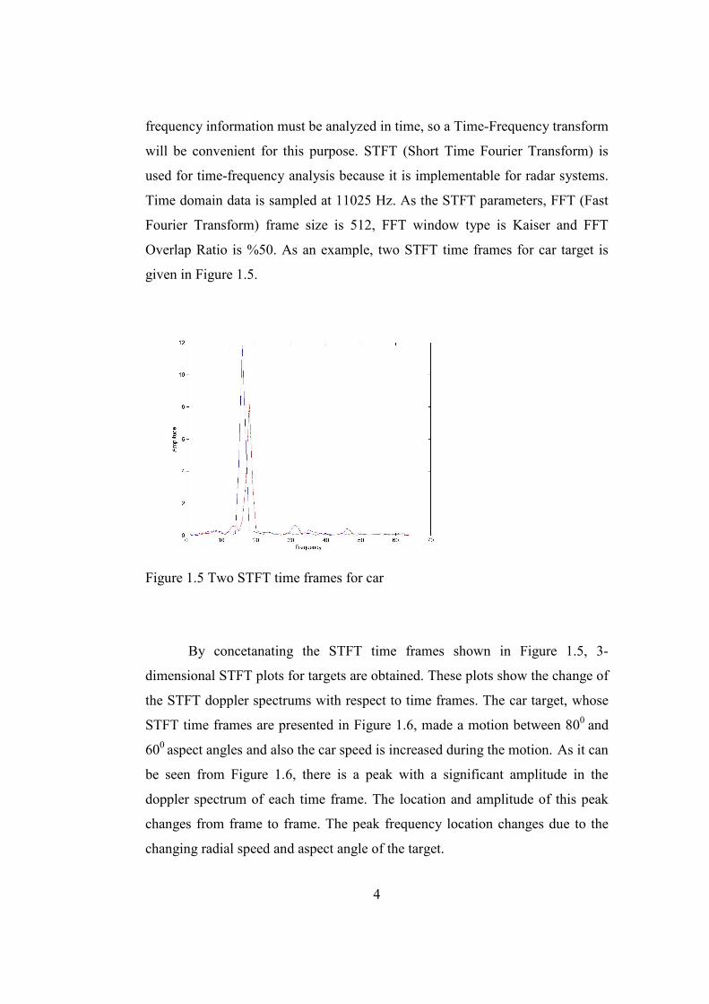
Overlap Ratio is %50. As an example, two STFT time frames for car target is

given in Figure 1.5.

Figure 1.5 Two STFT time frames for car

By concetanating the STFT time frames shown in Figure 1.5, 3-

dimensional STFT plots for targets are obtained. These plots show the change of

the STFT doppler spectrums with respect to time frames. The car target, whose

STFT time frames are presented in Figure 1.6, made a motion between 800 and

600 aspect angles and also the car speed is increased during the motion. As it can

be seen from Figure 1.6, there is a peak with a significant amplitude in the

doppler spectrum of each time frame. The location and amplitude of this peak

changes from frame to frame. The peak frequency location changes due to the

changing radial speed and aspect angle of the target.

5

Figure 1.6 3-dimensional STFT of a car.

The amplitude of the doppler spectrums change in time frames due to the

target range factor so doppler spectrum for each time frame must be normalized

in amplitude. For this purpose, amplitudes of frequency components of each

time frame are divided by the energy of that time frame. Amplitude

normalization step is explained in detail in Section 2.3. In Figure 1.7 the doppler

spectrums for time frames before amplitude normalization are shown. In Figure

1.8 the doppler spectrums of time frames after amplitude normalization are

shown.

6

Figure 1.7 3-dimensional STFTs for time frames before amplitude normalization

.

Figure 1.8 3-dimensional STFTs for time frames after amplitude normalization

After frame amplitude normalization, frequency information of doppler

spectrums must be normalized since target radial speed and aspect angle factors

changes the frequency information of doppler spectrums. The frame frequency

normalization step is explained in section 2.3. After frequency normalization of

time frames, the STFTs become in the form presented in Figure 1.9.

7

Figure 1.9 3-dimensional STFTs of time frames after frequency normalization

Amplitude and frequency normalized doppler spectrums of time frames

are called TRP (Target Recognition Pattern) vectors. TRP vectors form the

preprocessed doppler radar signals that can be used for classification.

In this thesis improving the performance of the doppler radar automatic

target classification system given in Erdogan (2002) is studied. The target types

are car, truck, bus, tank, helicopter, walking man and running man.

The main doppler radar target concept used in this thesis is Target

Recognition Pattern. Other useful doppler radar target concepts related to this

thesis are Target Doppler Signal and Target Doppler Spectrum.

Target Doppler Signal is the doppler signal received from the target.

Target Doppler Spectrum is the frequency spectrum of the Target

Doppler Signal.

Target Recognition Patterns are the normalized Target Doppler

Spectrums in Erdogan (2002) with respect to amplitude and frequency variations

which are triggered by target characteristics such as target range, target aspect

angle, target radial speed.

This thesis uses Target Recognition Patterns as input. Target

Recognition Patterns used in this thesis are the normalized Target Doppler

8

Spectrums of Target Doppler Signals obtained by the ASELSAN ASKARAD

Ground Surveillance Doppler Radar. (Appendix A)

1.1 Statement of the Problem

In some doppler radar systems, received doppler signals can also be

listened at the headphones of the radar operator as audio signal. Radar operators

can listen these signals to classifiy targets. However this task requires an extra

radar operator to perform only this job. Making the target classification in an

automatic manner could yield better classification performance and less operator

workload for such systems. The doctorate thesis Erdogan (2002) was such a

study to make the target the classification system of such a system (ASKARAD)

automatic.

The main goal of this thesis is to improve the classification performance

of the automatic target recognition system which was proposed during the

doctorate thesis study Erdogan (2002). In Erdogan (2002), even though a

classification based on neural networks was considered, the main challange of

the thesis was the preprocessing stage. We will use the preprocessing stage of

Erdogan (2002) and construct a target classification system that feeds multiple

time frames to classify the targets and increase the classification performance.

Time frames in Erdogan (2002) will be called as time bins in this thesis.

The goals of this thesis are:

• Constructing an automatic target recognition system that uses various

feature extraction and classification methods.

• To present the input data (Target Recognition Patterns) by considering

multiple time bins to the automatic target recognition system in order to

improve the classification performance of the system.

• Comparing the methods that are used for feature extraction and

classification according to the classification performance values of them.

9

• To test the performance of a classification scheme which uses multiple

classifiers organized hierarchically (Hierarchical Classification)

• To study target classification performance metrics such as clustering

quality, khat values and average recognition rate to use on the ATR

system classification results.

• To inspect the best ATR system parameters (feature extraction method,

classification method, data handling method and other system

parameters) to classifify car, truck, bus, tank, helicopter, walking man

and running man targets with a high classification performance value.

1.2 Scope of the Thesis

Some ATR system concepts are not in the scope of this thesis. These are listed

below:

• Data Acquisition stage of the ATR system is not implemented. This

thesis uses the acquired data of Erdogan (2002). There is no target

detection implementation, the target was detected by the operator. Also

target detection was done for single target conditions. The operations

done for data acquisition are explained in Chapter 2.

• Preprocessing stage of the ATR system is not implemented but the one

developed in Erdogan (2002) is used. The operations done for the

preprocessing is described briefly in Chapter 2.

The concepts that are in the scope of this thesis are listed below:

• Feature Extraction and Classification stages of the ATR system are

implemented.

• In the Feature Extraction stage of the ATR system, PCA, LDA, ICA and

NMF methods are implemented.

• In the Classification stage of the ATR system, KNN and SVM classifiers

are implemented.

10

• A Hierarchical Classification approach is also examined.

• Clustering Quality and Classification performance metrics are searched

and used.

• The TRP vectors obtained by considering multiple time bins are also

examined.

1.3 Contribution of the Thesis

In the traditional doppler ATR systems, the variations of the

preprocessed Target Doppler Spectrums in time are not evaluated (See Chapter

2 Background - Literature Survey part). This study examines the performance of

various feature extraction and classification methods and evaluates the effects of

using time variations of preprocessed Target Doppler Spectrums on the

classification performance.

1.4 Organization of the Thesis

The thesis is organized as follows:

Chapter 2 gives background on doppler radars, studies about doppler

radar ATR systems, a brief explanation about the prepocessing stage in Erdogan

(2002), pattern recognition, clustering quality measures, classification

performance metrics, feature extraction methods used in the thesis, classification

methods used in the thesis.

Chapter 3 explains the ATR system used in the thesis.

Chapter 4 gives the experimental results of the ATR system explained in

Chapter 3.

Chapter 5 gives conclusions and possible feature works.

11

CHAPTER 2

BACKGROUND

2.1 Background on Doppler Radars

Doppler Radars use the doppler effect to detect moving targets and

calculate the velocities of the targets. According to the doppler effect the relative

velocity of the target will create corresponding frequencies at the signal received

from the target (Richards, 2005). Doppler radars utilize these frequencies to

detect the target and find the characteristics of the target. This is due to the

common physical phenomenon that the phase of the reflected signal for a

stationary object is constant whereas for a moving object it is changing. The

change in the phase (doppler frequency shift) is proportional to the radial speed

of the target. The doppler frequency shift fd is given by the derivation:

fd = (2 * ft * vr) / c (2.1)

where

fd : Doppler frequency shift

ft : Frequency transmitted

vr : Radial speed of the target

c : Speed of the light

For approaching targets the doppler frequency shift will be added up to the

transmitted frequency and for diverging targets the doppler frequency shift will

be subtracted from the transmitted frequency. If the target has moving parts,

each distinct moving part of the target will create a different doppler frequency

on the received signal due to the different speeds of the different moving parts

of the target. This can be utilized to classify targets since different target types

show different motion characteristics.

12

In Table 2.1 physical structures for different target classes that will generate

doppler frequencies is presented.

Table 2.1 Structures for different target classes that generate doppler frequencies

TARGET CLASS STRUCTURE

Car Body and Wheels

Truck Body and Wheels

Bus Body and Wheels

Tank Body, Wheels and Track

Helicopter Body, Main and Back Propellers

Walking Man Body, Legs and Arms

Running Man Body, Legs and Arms

The most important factors that affect the received signal for a doppler

radar are target range, target aspect angle and target radial speed factors. These

factors were defined before. In Figure 2.1 we present these factors visually

(Erdogan, 2002).

13

Target’s Motion Direction

Target

Θ

Radar’s Line Of Sight

Θ: Target Aspect Angle R: Target Range

Radar

Target speed

Target radial speed

R

Figure 2.1 Doppler radar factors affecting the received signal

Target range affects the amplitude of the received signal, whereas target aspect

angle and target radial speed factors affect the frequency information of the

received signal.

2.2 Background on Doppler Radar ATR Studies

There are several studies performed on doppler radar automatic target

recognition. This section gives information about them.

In Castalez (1988), they classified 4 artillery munition classes with the

use of their doppler time signatures which were obtained by Hughes AN/TPQ-

37 radar. Back-Propagation Neural Network was used for classification and its

input was 15 doppler frequency bin amplitudes returned from the target and time

information which is fed to the 16. input. The 16-16-16 Back-Propagation was

trained with 32 samples for each target class and tested with 256 samples for

14

each class. Training samples were fed to the network for several thousand

cycles. The classification performance obtained was %92. They also used a 16-

32-32 network but same level of performance was obtained. In their experiments

they observed that three layer networks are sufficient and networks with more

layers can degrade the classification performance.

In Bullard (1991), classification of rotary wing aircraft was performed

based on the doppler signatures of the target. It was a study directed by MICOM

(U.S. Army Missile Command) / Georgia Tech measurements in 1989-90.

Target signatures of a Sikorsky S-55 helicopter were gathered with a high-pulse

repetition frequency X-band coherent radar. Helicopter’s main rotor blades, tail

rotor blades and hub regions creates distinct doppler signatures such that it

would be possible to identify helicopter characteristics such as rotor

configuration, blade count and rotor parity. This study did not implement an

automatic target classification system but it rather proposed methods to extract

information about rotary wing aircraft.

In Madrid (1992), an automatic target recognition system was designed

to classify four target types (airplanes and ground vehicles, helicopters, groups

of small moving targets (e.g, persons) and clutter). Doppler signatures were used

to implement the classification. The target classes were chosen in such a detail

to obtain an adequate classification performance. These target classes have

different spectral shape characteristics. Airplanes and ground vehicles do not

have any vibrating or rotating parts, they only have a large rigid body so their

signatures will include a large peak. Due to the main and tail rotor blades of the

helicopter, it will have flat wide sidebands around the sharp peak. In a group of

persons there will be members with different speeds. By considering the

spectrum of this class as the sums of individual member spectrums, there can be

more than one peak in the spectrum of this class. Since clutter has zero velocity,

its spectrum will consist of a peak at zero doppler.

At the signal processing stage each frame was transformed by Discrete

Fourier Transform. In the feature extraction step, four measurements including

15

shift of the spectral maximum and bandwidths at three different levels were

taken for each frame. The classifier is fed with 12 parameters which consist of

the features of three frames. The classifier was a 2 hidden layered Multilayer

Perceptron Neural Network with first and second hidden layers consist of 36 and

12 nodes respectively. For each target class, 200 samples were used at the test

phase of the experiment. Also some extra controls were performed under certain

conditions to prevent some kinds of errors. If aircrafts or group of persons had a

mean doppler shift of zero, such detections were labeled again as clutter. RCS

(Radar Cross Section) was utilized in some conditions such as the classification

of an accelerating plane as group of persons. After the feature extraction and

classification steps, for Aircraft/Vehicle and Helicopter target classes %100

classification performance were obtained while obtaining %97 and % 98

classification performances for Persons and Clutter target classes respectively.

% 2 of Persons classified as Aircraft/Vehicle and %1 classified as Clutter. % 2

of Clutter classified as Persons.

In Jianjun (1996), they performed aircraft target classification using by

using engine modulation on radar signatures obtained from the target. Radar

signatures were taken with an air defense surveillance radar. Target class set

consists of five aircrafts. Optical fourier transform was used for the extraction of

modulation signatures.

The classifier was a semi-connected backpropagation neural network

with one hidden layer. Numbers of training samples used for each target class

were 43, 45, 41, 39 and 60 respectively. Since there were not enough samples

for training samples, the leave-one-out technique is used for test. The

classification performances for five target classes were % 99.87, %98.67,

%99.33, %97.87 and % 98.27 respectively.

In Chen (2000), usefulness of micro-doppler signatures which are

induced by the rotating and vibrating parts of the target for target detection,

classification and recognition was considered. The modulations due to

vibrations are at low frequencies with respect to the body doppler frequency

16

while modulations due to rotations are at high frequencies with respect to the

body doppler frequency. In this study Time-Frequency Domain Signatures of

the targets such as stationary reflector, vibrating reflector, rotating blades and

walking-man with swinging arms were investigated and it was observed that

these targets have distinct time-frequency domain signatures which can be used

for target classification.

In Yoon (2000), they used time-frequency analysis to determine the

number of helicopter blades unambiguously. The main rotor rotation frequency

then can be estimated after the number of blades is determined and all of these

results can be used to determine the type of the helicopter. In the STFT of the

helicopter echoes there are N sinusoids corresponding corresponding to the N

rotor blades. They obtained satisfactory experiment results with a model

helicopter with changeable rotor blades.

In Stove (2002), they used the target data of the MSTAR (Man Portable

Surveillance and Tracking Radar) which is in use in U.K. and some other armed

forces since 1989. This radar has audio which can be used by the radar operator

to classify targets. The main aim of this study was to implement and test an

automatic target classifier which can be used to provide classification service to

the radar operator so that the workload of the radar operator can be reduced. The

target classes of interest were wheeled vehicles, tracked vehicles and personnel.

The sequences of audio samples were transformed by Fourier Transform. The

classifier used was Fisher Linear Discriminator whose inputs were normalized

spectrums. For a better performance, discrimination was implemented in two

stages. Personnel and vehicle classes were discriminated first then wheeled

vehicle and tracking vehicle classes were discriminated. %10 of the overall data

is used for testing. As the result of the experiment average correct classification

rates were % 86, % 83 and %83 for personnel, wheeled vehicles and tracked

vehicles respectively. The biggest confusion rate was between wheeled vehicle

and tracked vehicle classes. % 13 of the tracked vehicles classified as wheeled

and % 14 of wheeled vehicles classified as tracked.

17

In McConaghy (2003), they implemented an automatic target recognition

system that uses RBFNNs (Radial Basis Function Neural Networks) to classify

real life audio signals collected by a ground surveillance radar mounted on a

tank. With the implementation of such a system the number of personnels on the

tank will be reduced since this job is done by the personnel by listening to the

audio signals of the targets. In the neural network different signal classification

methods were used. First method was to use a linear autoregressive model to

extract the linear features of the audio data and second method was to use non-

linear predictors to model the audio data and then classify the signals according

to prediction errors. Target data was collected by AN/PPS-15 ground

surveillance radar and the target types of concern were men-marching, walking-

man, airplanes, trucks, tanks, crawling-man, birds and boats etc. By using a

linear adaptive algorithm for the training of the network, The RBF network can

be made implementable for real-time applications. % 75 of the overall data used

for training and %25 used for test. Classification Performance was %86 and %

65 for training and test data by using AR (Autoregessive) feature extraction.

Classification performance was %63 and %51 for training and test data by using

linear predictors. They also experimented classification with human

classification with a team of 40 humans and the classification performance was

%27.

In Lei (2005), they used Gabor filtering method to extract micro-doppler

signatures in the time-frequency domain. Dimension of the extracted features

was reduced by PCA. Bayes linear, k-nearest neighbor and SVM classifiers

were used and their classification performances were compared. This study used

Gabor function since it is a good tool for extracting localized features in both

spatial and frequency domain. Recognition rates were, between %44 and %92

for SVM, between %42 and %84 for KNN, between %38 and %78 for bayes

linear classifier. Recognition rates were low when the number of features was

below 500.

18

In Bilik (2005), they implemented an ATR system based on the Greedy

learning of GMM (Gaussian Mixture Model). The aim was to classify doppler

audio. Target class types were walking person(s), wheeled and tracked vehicles,

animal and clutter. Target class probability density functions were modeled by

GMMs. ML (Maximum Likelihood) and majority voting are used for

classification. Greedy-GMM based classification technique is implemented

using the linear predictive coding (LPC) and cepstrum coefficient feature sets,

extracted from the data. A classification rate of % 88 obtained with ML

classifier and %96 obtained with majority voting classifier.

2.3 Data Acquisition and Preprocessing

In this section data acquisition and preprocessing done in Erdogan

(2002) for ASKARAD target signals are explained. The outputs of the

prepocessing stage are TRP vectors which are also input to our target

recognition system.

2.3.1 Data Acquisition

Doppler Signal is obtained from a range. This received signal is

processed in the radar receiver in order to make it suitable for the target

detection. In ASKARAD, doppler signal can also be listened by the radar

operator as an audio signal. The audio signal is recorded as an analog signal,

digitized at 11025 Hz and saved as 8 bit mono wav file. Information such as

target range and azimuth can not be obtained from this signal.

2.3.2 Preprocessing of Signals

For a doppler radar there are several factors affecting the received target

doppler signal. Most important of them are target range, target aspect angle and

target radial speed. Target range is the distance between the target and the radar.

Target aspect angle is the angle between the direction of the motion of the target

19

and line of sight of the radar. Target Radial Speed is the target speed component

along the line of sight of the radar. Target range affects the amplitude

information of the received doppler signal, target speed and target aspect angle

factors affect the frequency information of the received doppler signal. Since

target speed and aspect angle can change in time, frequency analysis must be

done in time.

Each audio signal received at a time-bin is transformed into frequency

domain by using STFT (Short Time Fourier Transform). This transformed signal

can be called as STFT frame. In Figure 2.2 STFT frames for a walking man

target are presented.

Figure 2.2 3-dimensional STFT frames of Walking Man

20

As mentioned previously the input to the ATR system designed in the

thesis are the TRP vectors. In the following paragraphs, the preprocessing steps

applied in order to obtain TRP vectors are explained.

Amplitude Normalization is done for each STFT frame by dividing

amplitudes of the frequency components for an STFT frame by the frame

energy.

After frame amplitude normalization step, frequency normalization is

performed. The aim of this step is to find the TCB (Target Characteristics Band)

for each STFT frame. Target Characteristics Band can be defined as the part of

the STFT spectrum where the target characteristics reside. TCB can be

expressed by mean frequency and TCB width.

The mean frequency of a STFT frame is:

Mean Frequency = ((Frame Amplitudes Vector)3 * Frame Bin Vector) /

(∑ Frame Bin Vector) (2.2)

where

Frame Bin Vector = [1, 2,.., Frame Length]

The average of the mean frequencies of the STFT frames is defined as

the mean frequency of STFT frames. Mean frequency averaging is done on a

specified number of consecutive frames. TCB is located at the mean frequency

and its width is set equal to the twice of the mean frequency.

As the last step in the prepocessing stage, TCB frame is transformed into

fixed length TRP vector. TRP vectors form the basis for feature extraction since

target doppler signal is amplitude and frequency normalized and characteristic

part of the frequency spectrum is extracted regardless of the actual frequency

components. The dimension of TRP vector is chosen as 63.

21

2.4 Data Used in the Thesis

This thesis uses the Target Recognition Patterns (preprocessed Target

Doppler Spectrums of ASELSAN ASKARAD Ground Surveillance Doppler

Radar Target Signals). Half of TRP vectors are used for training and half of

them used for testing. The Data Acquisition and Preprocessing done in is

explanied in section 2.3.

TRP vectors used for training are presented in Figures 2.3 to 2.9. The

data dimension of each time bin is 63.

Figure 2.3 TRP vectors of training data for CAR class

22

Figure 2.4 TRP vectors of training data for TRUCK class.

Figure 2.5 TRP vectors of training data for BUS class

23

Figure 2.6 TRP vectors of training data for TANK class

Figure 2.7 TRP vectors of training data for HELICOPTER class

24

Figure 2.8 TRP vectors of training data for WALKING MAN class.

Figure 2.9 TRP vectors of training data for RUNNING MAN class

25

A total of 884 TRP vectors are used in this thesis. The number of TRP vectors

for car, truck, bus, tank, helicopter, walking man and moving man classes are

104, 114, 188, 30, 42, 218 and 188 respectively. Half of the TRP vectors are

used for training and half of them are used for test.

2.5 Background on Pattern Recognition

Pattern recognition aims to assign a measurement, object or data to one

of the classes defined. Mainly a pattern recognition system consists of three

stages which are data gathering, feature extraction and classification. Data

gathering part or the sensor part gathers the raw data or takes the measurements

that will be the input to the feature extraction part. Depending on the type of

gathered data, there can be need of preprocessing for the data. This can be due to

the noise or some other factors that are special to the data. The aim of the feature

extraction part is to extract characteristic and relevant information (also can be

called as features) from the raw data. Extracted features are input to the

classification stage. The classification stage assigns the data or object to one of

the defined classes based on the extracted features. The classification can be

either supervised or unsupervised. In supervised classification there is a training

data set which consists of classified data and the test data is classified according

to this training data. In unsupervised classification, there is no priori

information; classification is done based on the statistical information of the

data.

2.6 Performance Measures

One of the main areas of interest in Pattern Recognition systems is to

represent the performance of the feature extraction step mathematically in order

to evaluate the feature extraction method performance separately from the

classifier. To perform this, Clustering Quality Measures can be used. A

26

clustering quality measure can be defined as a function whose input is a sample

set and partition of the samples to the clusters and whose output is a number that

represents the quality of clustering.

One of the CQMs (Clustering Quality Measures) is given in Schweitzer

(1999). This measure is defined as the ratio of Sw (Within Class Scatter Matrix)

to Sb (Between Class Scatter Matrix).

CQM = Sw / Sb (2.3)

The Sb (Between Class Scatter Matrix) and Sw (Within Class Scatter

Matrix) are defined as

Sb = ∑j (mj)(µj - µ)(µj - µ)T j = 1..k (2.4)

Sw = ∑j ∑i (xi - µj)(xi - µj)T i = 1..Gj (2.5)

The definition of mean of all samples is given below.

µ = (∑j (mj µj )) / m j = 1..k (2.6)

where

k : Number of clusters.

G1..Gk : Partition of the patterns into k clusters.

mj : Number of samples in cluster j.

xi : Samples in cluster j.

µ1.. µ k : Means of the clusters.

µ : Mean of all samples.

m : Number of all samples.

A smaller value of the clustering quality measure Sw / Sb indicates a

better clustering quality value since a smaller value of Sw and a larger value of

Sb denotes a good clustering. Samples in a single cluster must be closer to each

other and clusters must be far from each other for a good clustering.

Other clustering quality measure is given in Zardoshti (1993). This

clustering quality measure is defined as cluster-to-cluster similarity. The cluster-

to-cluster similarity value between two clusters is the ration of the difference of

27

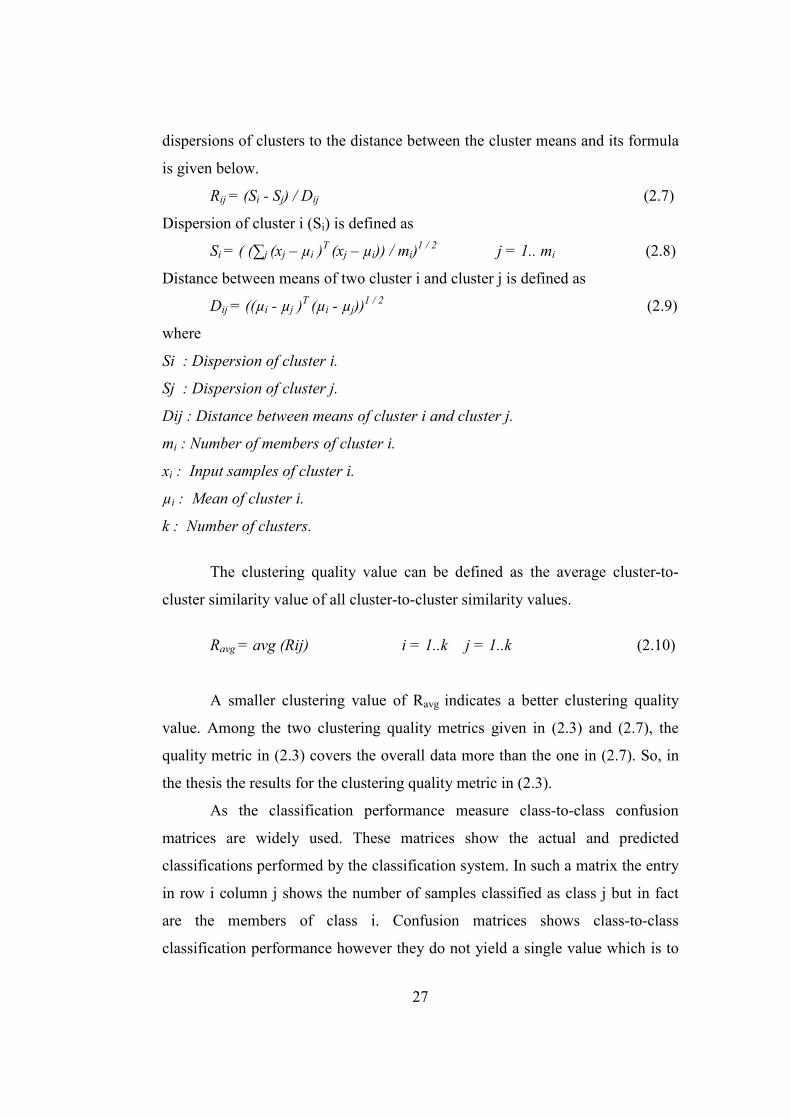
dispersions of clusters to the distance between the cluster means and its formula

is given below.

Rij = (Si - Sj) / Dij (2.7)

Dispersion of cluster i (Si) is defined as

Si = ( (∑j (xj – µi )T

(xj – µi)) / mi)1 / 2

j = 1.. mi (2.8)

Distance between means of two cluster i and cluster j is defined as

Dij = ((µi - µj )T

(µi - µj))1 / 2 (2.9)

where

Si : Dispersion of cluster i.

Sj : Dispersion of cluster j.

Dij : Distance between means of cluster i and cluster j.

mi : Number of members of cluster i.

xi : Input samples of cluster i.

µi : Mean of cluster i.

k : Number of clusters.

The clustering quality value can be defined as the average cluster-to-

cluster similarity value of all cluster-to-cluster similarity values.

Ravg = avg (Rij) i = 1..k j = 1..k (2.10)

A smaller clustering value of Ravg indicates a better clustering quality

value. Among the two clustering quality metrics given in (2.3) and (2.7), the

quality metric in (2.3) covers the overall data more than the one in (2.7). So, in

the thesis the results for the clustering quality metric in (2.3).

As the classification performance measure class-to-class confusion

matrices are widely used. These matrices show the actual and predicted

classifications performed by the classification system. In such a matrix the entry

in row i column j shows the number of samples classified as class j but in fact

are the members of class i. Confusion matrices shows class-to-class

classification performance however they do not yield a single value which is to

28

show the overall performance of the classifier. In the literature there are some

classification performance values used for this purpose. One of them is called

KHAT (Wilkinson, 2005). This classification performance metric takes the

class-to-class confusion matrix as input and returns a single value that presents

the classification performance. KHAT value of a confusion matrix is given by:

( N * ( ∑i Xii ) ) – ( ∑i (Xi+ * X+i) ) i = 1..r (2.11)

KHAT = ______________________________________

( N2

) – ( ∑i (Xi+ * X+i) )

where r : Number of rows in the confusion matrix

Xii : Number of observations in row i column i of the confusion

matrix

Xi+ : Marginal total of row i of the confusion matrix

X+i : Marginal total of column i of the confusion matrix

N : Total number of samples in the confusion matrix

KHAT formula takes into account not only the correct classifications but

also the misclassifications.

Also the average of the correct classification rates of each class can also

be used as classification metric and its formula is given below.

Recognitionavg = ( ∑i Ci ) / k (2.12)

where

Ci = Correct recognition rate for class i

k = Number of classes

In fact Recognitionavg given in (2.12) is the sum of the diagonal elements in

confusion matrix divided by the number of classes.

29

2.7 Feature Extraction and Classification Methods

In this thesis, PCA, LDA, ICA and NMF methods are used for feature

extraction, while KNN and SVM methods are used for classification. Our target

recognition system consists of a feature extraction method and a classifer chosen

from these methods. Methods are explained in the following sections.

2.7.1 PCA

PCA (Principal component analysis) is a non-parametric method that

extracts relevant information from complex data sets. The main aim of PCA is

to reduce the dimension of the data while preserving as much representative

information as the original data (Shlens, 2005). PCA is a linear transformation

that computes a matrix which transforms the high dimensional space to a lower

dimensional space. PCA transforms the data along the directions where data

varies the most. PCA is unsupervised, i.e. it does not deal with class information

of the data.

Considering the vector x, PCA tries to find the matrix T ∈ RKxN for

which y = Tx where y ∈ RK is the transformed version of x∈ RN such that

K < N.

PCA method can be summerized as below:

• x1,x2 .. xL are the sample vectors whose dimension is N and will be

reduced. L is the number of samples.

• Calculate the mean of the samples. µ = (∑j xj) / L j = 1..L

• Subtract the mean from the samples. Фj = xj - µ

• Calculate the matrix A. A = [Ф1 Ф2 .. ФL]

• Calculate the covariance matrix C = AAT

• Calculate the eigenvalues of C, Λ1 > Λ2 > .. > ΛN

• Calculate the eigenvectors of C, Π1, Π2, .. ,ΠN

• Eigenvectors determines the directions of the new space.

30

• Any training or test sample can be projected to the new space by

yi = (xi - µ) [Π1 Π2 .. ΠK] where xi is the sample and yi is the transformed

sample.

• Dimensionality reduction means loss of information. The dimension of

the new space must be chosen such that the difference between yi and xi

must be minimum.

• In order to minimize the difference between yi and xi , K must be

chosen such that;

(∑i Λi) / (∑j Λj ) > Threshold (For example 0.85)

where i = 1 .. K and j = 1 .. N

• One advantage of PCA is that noisy directions can be eliminated from

data representation.

2.7.2 LDA

LDA (Linear Discriminant Analysis) is a feature extraction method that

utilizes the class information of the samples. LDA tries to find the directions in

which separation of classes is good by computing the within class scatter Sw and

between class scatter SB (Shan, 2002).

Within class scatter Sw is given by the derivation:

Sw = ∑i ∑j (yj - µi) (yj - µi)T

i = 1..k j = 1..mi (2.13)

where

k : Number of classes

mi : Number of samples that belongs to class i

µi : Mean of the samples in class i

Between class scatter SB is given by derivation:

SB = ∑i (µi - µ) (µi - µ))T (2.14)

31

where

µ : Mean of the overall data set

LDA is a transformation that maximizes between class scatter while minimizing

within class scatter. To perform this LDA finds the optimal transformation W to

maximize J(W). J(W) is given by the derivation:

J(W) = (WT SB W) / (W

T SW W) (2.15)

To maximize J(W) the equation below must be solved.

SBW = Λ SWW (2.16)

For the equation (2.16) to have a solution, SW must be non-singular. Solving

equation (2.16) requires finding the eigenvectors of SW-1

SB. In our target

recognition system we reduced the dimension of the training and test samples to

32 with PCA before applying LDA.

2.7.3 ICA

ICA (Independent Component Anlaysis) is a recently developed linear

transformation method that maximizes the statistical independence of the

components of the new representation as much as possible (Hyvarinen, 1999).

ICA can be defined in a general sense as a linear transformation method which

finds a projection W for a random vector x such that s = Wx and components of

s are statisticaly independent as much as possible. ICA is mainly used for blind

source separation problem and it can also be used for feature extraction. ICA

can be considered as a variant of PCA such that PCA makes the data

uncorrelated whereas ICA makes the data statistically independent (Lathauwer,

2000). The aim of ICA is to make the transformed data non-gaussian Vasilescu

(2005).

To implement ICA, the code in Ustun (2007) is used with modifications.

Before executing ICA, we reduced the size of training and test samples to 32

with PCA.

32

2.7.4 NMF

NMF (Non-negative Matrix Factorization) is used in many areas. In

algebra, large and complex problems can be divided to small simple

subproblems by NMF. In pattern recognition NMF can be used for feature

extraction and dimension reduction (Weixiang, 2006). Considering an nxm non-

negative matrix V, the aim of NMF is to find two non-negative matrices W and

H such that

V ≈ W * H (2.17)

where

W ∈ Rnxr

, H ∈ Rrxm

Here, r is generally chosen smaller than n and can be as small as possible to

reduce dimension (Xue, 2006). W and H are also non-negative.

To find matrices W and H, there are different methods in the literature.

In the thesis we used the one that minimizes Divergence(V||WH) with respect to

W and H, being subject to the constraints W > 0 and H > 0. In order to satisfy

the non-negativity constraint for V, W and H, during the experiments we added

the minimum value of V to all training and test samples. W and H can be

intiated to random values. The update rules for W and H are given by

derivations:

Haµ ← Haµ (∑i (Wia Viµ / (WH) iµ)) / (∑k Wka) (2.18)

Wia ← Wia (∑µ (Haµ Viµ / (WH) iµ)) / (∑v Hav) (2.19)

Pseudo inverse of matrix W is multiplied by test samples and transpose

of matrix H gives the NMF applied training samples. In our pattern recognition

system before executing NMF, dimension of training and test samples are

reduced to 32 with PCA.

33

2.7.5 KNN

KNN (K nearest neighbor) is a classifier that classifies test samples

according to the class labels of training samples that are closest to the test

sample in the feature space. The class label of the test sample is decided as the

most common class label among the class labels of the K-nearest neighbors. It

can be considered as the simplest classifier. In our target recognition system, test

samples are classified according to the class labels of the 5 closest training

samples. KNN can not be considered as a real time implementable classifier

since at execution, for a test sample distances to all training samples are

calculated rather than multiplying the sample with a matrix and deciding the

class label. There is no training phase for this classifier.

2.7.6 SVM

A SVM (Support Vector Machine) is a classifier that separates the data

into two groups by forming an N dimensional hyperplane. The aim of SVM is to

find the optimal separating hyperplane so that different classes are on the

different sides of the hyperplane. Support vectors are the samples which are the

closest ones to the hyperplane. SVMs are used for handwritten digit recognition,

object recognition, speaker identification, face detection, text categorization

(Burgess, 1998). For the 2-dimensional case, an example separating hyperplane

and support vectors are presented in Figure 2.10.

34

Figure 2.10 Separating hyperplane for 2 dimensions

In Figure 2.10 the green and blue labels shows the samples of two

different classes. The continuos black line is the separating hyperplane and the

samples that are closest to the two dashed lines are the support vectors. This is a

compleletely separable condition i.e SVM separates all of the samples correctly

to their classes, there is no overlapping. There can be non-separable cases in

which SVM can not separate the classes and there will be training errors too.

SVM finds the support vectors for which the margin between clusters is

maximized. The aim of maximizing the margins is to reduce the testing errors.

For the cases when the boundaries between the clusters are so complex that

linear seperation is not possible, non-linear kernel functions can be used instead

of linearly separating hyperplanes. Radial Basis Function is one of the most

recommended and used one as the kernel function and we also used it in our

code. The support vector machine code used in the thesis is given in Spider

(2006).

35

CHAPTER 3

THE PROPOSED ATR SYSTEM

3.1 The General Structure of the ATR System

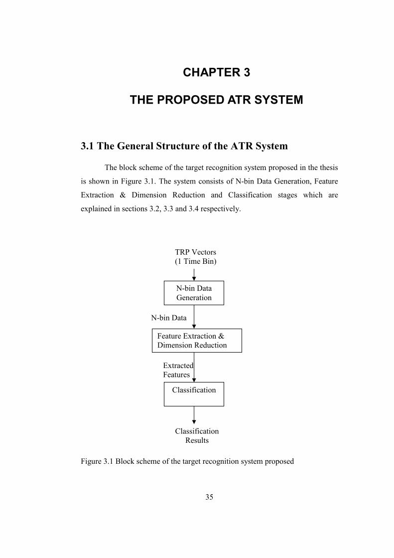
The block scheme of the target recognition system proposed in the thesis

is shown in Figure 3.1. The system consists of N-bin Data Generation, Feature

Extraction & Dimension Reduction and Classification stages which are

explained in sections 3.2, 3.3 and 3.4 respectively.

Figure 3.1 Block scheme of the target recognition system proposed

N-bin Data Generation

TRP Vectors (1 Time Bin)

Feature Extraction & Dimension Reduction

Classification

N-bin Data

Extracted Features

Classification Results

36

3.2 N-bin Data Generation

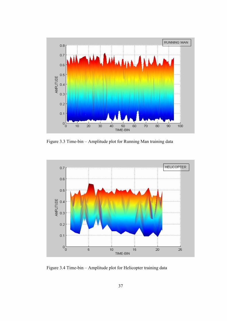
Some target classes have repetitions in time in their TRP vectors. To see

these repetitions in time visually, 3-D plots of TRP vectors of target training

classes were given in the figures from Figure 2.3 to Figure 2.9.

From the figures we can observe that TRP vectors of vehicles (car, truck,

bus) are homogenic in time while target classes such as walking man, running

man and helicopter have different vectors which repeat itself in time. To see

these repetitions in detail furtherly 2-D time-bin – amplitude plots for walking

man, running man and helicopter targets are shown below in Figure 3.2 to

Figure 3.4. These plots are the projections of the 3-D plots in Figure 2.8, Figure

2.9 and Figure 2.7 into amplitude and time-bin axes. One of the main goals of

this thesis is to take into consideration these repetitions in time in order to

enhance classification performance.

Figure 3.2 Time-bin – Amplitude plot for Walking Man training data

37

Figure 3.3 Time-bin – Amplitude plot for Running Man training data

Figure 3.4 Time-bin – Amplitude plot for Helicopter training data

38

To take these repetitions into consideration, successive TRP vectors in

time of a target can be concatenated and presented to the feature extraction part

of the target recognition system. The N-bin Data Generation part of the target

recognition system just concatenates previous N-1 TRP vectors with the current

TRP vector and outputs this as the N time-bin sample.

3.3 Feature Extraction & Dimension Reduction

The second part of the target recognition system is feature extraction and

dimension reduction part. PCA, LDA, ICA, NMF methods are used

alternatively for feature extraction. Before applying LDA, ICA and NMF

methods, we used PCA for dimension reduction. Data dimension is reduced with

PCA to 32 before applying these algorihms. Feature extraction part is shown in

Figure 3.5. After the feature extraction step not all the features of the samples

are fed to the classifier, they are further reduced to proper dimension.

Figure 3.5 Feature Extraction & Dimension Reduction of the target recognition

system

PCA

LDA NMF ICA

Dimension Reduction

N-bin Data

Extracted Features

Feature Extraction & Dimension Reduction

39

3.4 Classification

K-Nearest Neighbor and Support Vector Machine classifiers are used at the

classification stage of the pattern recognition system. Multi-Layer Perceptron

classifier is not used in classification because for target classes which have less

training samples than other classes (tank and helicopter), poor classification

performance results are obtained. KNN classifier is coded in MATLAB and we

used an SVM tool that we found from the internet Spider (2006).

Figure 3.6 Classification stage of the pattern recognition system

3.5 Hierarchical Classification

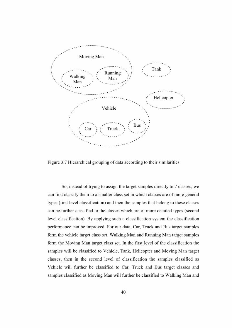
Observing the training TRP vectors shown in Figure 2.3 to Figure 2.9,

we see that some target classes have similar vectors compared to the other

classes. While Car, Truck and Bus TRP vectors are similar to each other and

make one group, the Walking Man and Running Man TRP vectors make another

group. This grouping is shown schematically in Figure 3.7

KNN

SVM

Extracted Features

Classification Results

Classification

40

Moving Man

Tank

Helicopter

Running Man Walking

Man

Vehicle

Car Truck Bus

Figure 3.7 Hierarchical grouping of data according to their similarities

So, instead of trying to assign the target samples directly to 7 classes, we

can first classify them to a smaller class set in which classes are of more general

types (first level classification) and then the samples that belong to these classes

can be further classified to the classes which are of more detailed types (second

level classification). By applying such a classification system the classification

performance can be improved. For our data, Car, Truck and Bus target samples

form the vehicle target class set. Walking Man and Running Man target samples

form the Moving Man target class set. In the first level of the classification the

samples will be classified to Vehicle, Tank, Helicopter and Moving Man target

classes, then in the second level of classification the samples classified as

Vehicle will further be classified to Car, Truck and Bus target classes and

samples classified as Moving Man will further be classified to Walking Man and

41

Running Man target classes. The overall hierarchical classification system for

our target samples is shown in Figure 3.8.

Figure 3.8 Hierarchical target recognition system

Feature Extraction-1

Classifier-1

Vehicle Tank Helicopter Moving Man

Feature Extraction-2.1

Classifier-2.1

Feature Extraction-2.2

Classifier-2.2

Car Truck

Bus

Walking Man

Running Man

TRP Vectors

Tank Helicopter

First Level Classification

Second Level Classification

42

The Feature Extraction steps shown in Figure 3.8 can be PCA, LDA,

ICA or NMF as before we used in Section 3.3 and the Classifier steps can ve

SVM or KNN similarly as in Section 3.4. Vehicle, Tank, Helicopter and Moving

Man target train and test samples are fed to the Feature Extraction-1 step.

Feature Extraction-1 uses vehicle, tank, helicopter and moving man classes as

base classes. Classifier-1 is also trained with extracted features of the training

samples of these classes. After Classifier-1, all target test samples are classified

to vehicle, tank, helicopter and moving man target classes.

TRP vectors of target test samples classified as Vehicle are then

classified as Car, Truck, Bus after Feature Extraction-2.1 and Classifier-2.1

steps. Feature Extraction-2.1 step uses Car, Truck and Bus base classes.

Classifier-2.1 is trained with the extracted features of target train samples

belonging to the mentioned classes.

TRP vectors of target test samples classified as Moving Man are then

classified as Walking Man and Running Man after Feature Extraction-2.2 and

Classifier-2.2 steps. Feature Extraction-2.2 uses Walking Man and Running

Man as base classes. Classifier-2.2 is trained with the extracted features of target

train samples belonging to the mentioned classes.

The khat result tables and recognition rates of hierarchical classification

for various time-bin and principal component values are presented in Chapter 4.

43

3.6 Clustering and Classification Performance Analysis

To evaluate the performance of target recognition system shown in

Figure 3.1, Clustering Quality Evaluations and Classification Performance

Evaluations metrics are applied which are described in 3.6.1 and 3.6.2

respectively.

3.6.1 Clustering Quality Evaluation

Before observing the overall target recognition system classification

performance, we used simply the PCA method for 1 time-bin, 5 time-bin and 10

time-bin data in order to see the affect of repetitions in time. In our normalized

data set, a single time bin contains 63 data points in the frequency domain. So,

data dimensions for 1 bin data, 5 bin data and 10 bin data are 63, 315 and 630

respectively. In the dimension reduction step we reduced the size of extracted

features to 2 for visual examination. The separation of target classes for train

and test data with respect to these 2 extracted features is shown in Chapter 4.

Observing the affect of using repetitions in time visually by using 2-D

plots of the 2-dimensional extracted features gives us an intuition on how the

samples are distribured over the feature space when different numbers of bins

are used. However expressing it mathematically is a better way. For this purpose

we used the clustering quality metrics in (2.3) and (2.7). After N-bin Data

Generation and Feature Extraction & Dimension Reduction steps, we calculated

the values of these clustering quality metrics on the feature vectors obtained.

Clustering quality values are calculated for various time-bin data and for various

numbers of principal components (By the number principal components we

refer to the dimension of feature vectors after the N-bin Data Generation and

Feature Extraction & Dimension Reduction steps.). Values calculated according

to the metric in (2.3) are presented in Chapter 4.

44

3.6.2 Classification Performance Evaluation

By feeding our test TRP vectors to the target recognition system shown

in Figure 3.1 and which is trained with our training TRP vectors, we obtained

class-to-class confusion matrices. To express the classification performance as a

single value, KHAT classification performance metric is used, which is

described in section 2.6. Class-to-class confusion matrices are input to the

KHAT function and KHAT function returns a single value that represents the

classification performance. A higher value represents a better classification.

Maximum value of KHAT is 1 which means that there are no misclassifications.

KHAT values and Recognition Rates for different number of time bins and

number of principal components are presented in Chapter 4.

45

CHAPTER 4

EXPERIMENTAL RESULTS

In this chapter clustering quality results and classification performance

results which were explained in Chapter 3 are presented.

4.1 Clustering Quality Results

To see the effects of using repetitions in the TRP vectors before performing all

of the target recognition system steps, we applied PCA feature extraction

method to 1, 5 and 10 time-bin data for target training and test data sets. When

applying PCA to training and test data sets, the coefficients calculated for the

training data set are used. After applying PCA, we presented the 2-D plots of the

first two principal components having the largest eigen values through Figure

4.1 to Figure 4.6.

Figure 4.1 Target clusters of train data set for 1 bin data with PCA reduced

components.

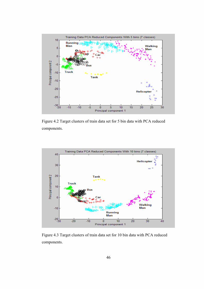
46


components.


components.

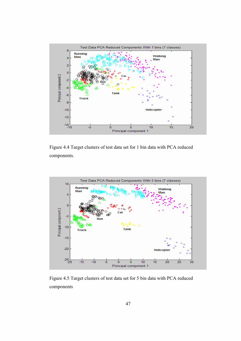
47

Figure 4.4 Target clusters of test data set for 1 bin data with PCA reduced

components.


components

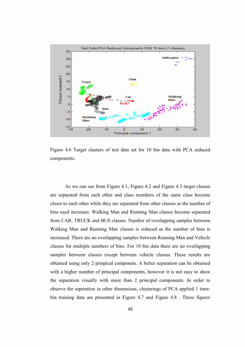
48


components.

As we can see from Figure 4.1, Figure 4.2 and Figure 4.3 target classes

are separated from each other and class members of the same class become

closer to each other while they are separated from other classes as the number of

bins used increases. Walking Man and Running Man classes become separated

from CAR, TRUCK and BUS classes. Number of overlapping samples between

Walking Man and Running Man classes is reduced as the number of bins is

increased. There are no overlapping samples between Running Man and Vehicle

classes for multiple numbers of bins. For 10 bin data there are no overlapping

samples between classes except between vehicle classes. These results are

obtained using only 2 prinpical componets. A better separation can be obtained

with a higher number of principal components, however it is not easy to show

the separation visually with more than 2 principal components. In order to

observe the seperation in other dimensions, clusterings of PCA applied 1 time-

bin training data are presented in Figure 4.7 and Figure 4.8 . These figures

49

-10 -5 0 5 10 15-8

-6

-4

-2

0

2

4

6Training Data PCA Reduced Components With 1 bins (7 classes)

Principal Component 1

Principal Component 3 Truck

Car

Helicopter

Walking

Man

Running

Man

Bus

Tank

-14 -12 -10 -8 -6 -4 -2 0 2 4 6-8

-6

-4

-2

0

2

4




Helicopter

Tank

Bus

Walking

Man

Running

Man

Car

Truck

present the clusterings with respect to first-third and second-third principal

components.

Figure 4.7 Target clusters of PCA applied training data set for 1 bin data with

respect to first and third principal components


respect to second and third principal components

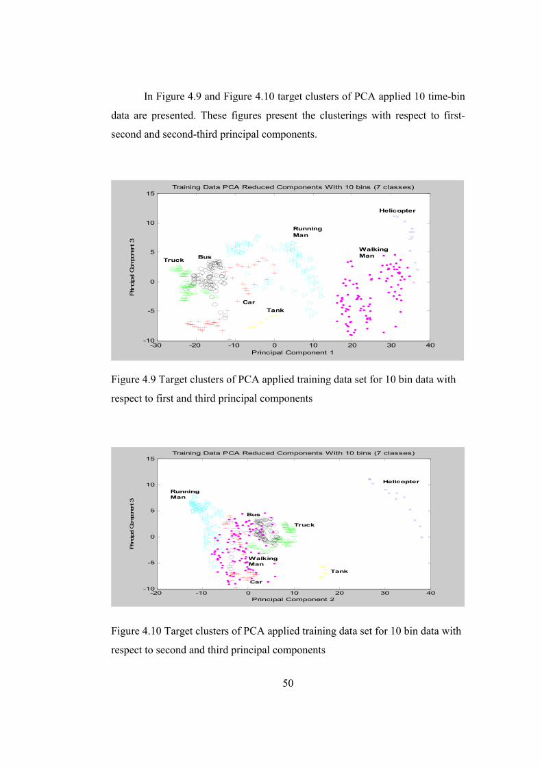
50

-20 -10 0 10 20 30 40-10

-5

0

5

10




Helicopter

Running

Man

Car

Tank

Truck

Walking

Man

Bus

-30 -20 -10 0 10 20 30 40-10

-5

0

5

10




Running

Man

Walking

Man

Helicopter

Tank

TruckBus

Car

In Figure 4.9 and Figure 4.10 target clusters of PCA applied 10 time-bin

data are presented. These figures present the clusterings with respect to first-

second and second-third principal components.


respect to first and third principal components


respect to second and third principal components

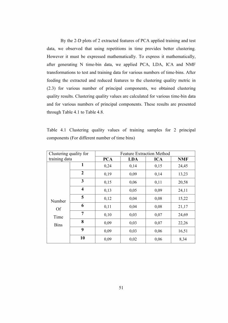
51

By the 2-D plots of 2 extracted features of PCA applied training and test

data, we observed that using repetitions in time provides better clustering.

However it must be expressed mathematically. To express it mathematically,

after generating N time-bin data, we applied PCA, LDA, ICA and NMF

transformations to test and training data for various numbers of time-bins. After

feeding the extracted and reduced features to the clustering quality metric in

(2.3) for various number of principal components, we obtained clustering

quality results. Clustering quality values are calculated for various time-bin data

and for various numbers of principal components. These results are presented

through Table 4.1 to Table 4.8.


components (For different number of time bins)

Feature Extraction Method Clustering quality for

training data PCA LDA ICA NMF 1 0,24 0,14 0,15 24,45

2 0,19 0,09 0,14 13,23

3 0,15 0,06 0,11 20,58

4 0,13 0,05 0,09 24,11

5 0,12 0,04 0,08 15,22

6 0,11 0,04 0,08 21,17

7 0,10 0,03 0,07 24,69

8 0,09 0,03 0,07 22,26

9 0,09 0,03 0,06 16,51

Number

Of

Time

Bins

10 0,09 0,02 0,06 8,34

52

Table 4.2 Clustering quality values of test samples for 2 principal components

Feature Extraction Method Clustering quality for test data PCA LDA ICA NMF

1 0,31 0,19 0,20 21,51

2 0,25 0,11 0,18 15,54

3 0,22 0,09 0,15 17,31

4 0,19 0,07 0,13 27,12

5 0,17 0,06 0,12 15,32

6 0,16 0,05 0,11 27,15

7 0,15 0,04 0,11 20,49

8 0,14 0,04 0,11 19,99

9 0,14 0,04 0,10 16,56

Number

Of

Time

Bins

10 0,14 0,03 0,10 8,72


components



2 0,23 0,11 0,13 11,89

3 0,19 0,09 0,11 12,15

4 0,17 0,07 0,09 22,43

5 0,16 0,06 0,08 17,81

6 0,15 0,05 0,08 11,34

7 0,14 0,04 0,07 17,88

8 0,12 0,04 0,07 13,16

9 0,12 0,04 0,06 12,82

Number

Of

Time

Bins

10 0,11 0,03 0,06 9,89

53



test data PCA LDA ICA NMF 1 0,35 0,22 0,21 13,18

2 0,28 0,16 0,18 11,09

3 0,24 0,12 0,15 11,27

4 0,22 0,10 0,14 17,20

5 0,21 0,08 0,12 17,40

6 0,20 0,07 0,12 10,08

7 0,18 0,06 0,11 18,69

8 0,17 0,06 0,11 11,32

9 0,16 0,05 0,10 12,10

Number

Of

Time

Bins

10 0,15 0,05 0,10 10,33


components

Feature Extraction Method Clustering quality for training data PCA LDA ICA NMF

1 0,35 0,17 0,16 18,80

2 0,28 0,15 0,13 19,69

3 0,24 0,11 0,11 13,10

4 0,22 0,09 0,09 18,12

5 0,20 0,08 0,08 13,49

6 0,18 0,07 0,07 15,16

7 0,17 0,06 0,07 10,95

8 0,16 0,05 0,07 15,65

9 0,15 0,05 0,06 11,14

Number

Of

Time

Bins

10 0,14 0,04 0,06 9,68

54


Feature Extraction Method Clustering quality for test data PCA LDA ICA NMF

1 0,39 0,27 0,21 13,48

2 0,33 0,21 0,18 21,17

3 0,29 0,15 0,15 11,51

4 0,27 0,12 0,13 15,01

5 0,25 0,10 0,13 12,14

6 0,23 0,08 0,11 12,01

7 0,22 0,07 0,11 10,73

8 0,21 0,07 0,11 16,48

9 0,20 0,06 0,10 12,16

Number

Of

Time

Bins

10 0,19 0,06 0,10 9,77


components



2 0,31 0,17 0,13 13,90

3 0,26 0,13 0,10 16,40

4 0,24 0,11 0,09 12,71

5 0,23 0,09 0,08 11,03

6 0,22 0,08 0,07 13,45

7 0,20 0,07 0,07 9,91

8 0,19 0,06 0,07 11,81

9 0,19 0,06 0,06 12,07

Number

Of

Time

Bins

10 0,18 0,05 0,06 11,85

55



test data PCA LDA ICA NMF 1 0,41 0,31 0,21 12,56

2 0,35 0,24 0,18 13,92

3 0,31 0,18 0,15 13,86

4 0,30 0,14 0,13 12,22

5 0,28 0,12 0,12 10,71

6 0,27 0,10 0,11 11,96

7 0,26 0,09 0,11 10,49

8 0,25 0,08 0,10 12,00

9 0,24 0,07 0,10 13,11

Number

Of

Time

Bins

10 0,23 0,07 0,10 11,53

Due to the clustering quality description in (2.3), a smaller value

represents a better clustering quality. As we can see from Table 4.1 to Table 4.8,

increasing the number of time-bins provides a better clustering quality for all

feature extraction methods. Among the feature extraction algorithms applied,

LDA provides the best clustering quality and NMF provides the worst clustering

quality. As an example, for Training Data of 10 time-bins which is reduced to 5

principal components with feature extraction, we get 11.53, 0.18, 0.06 and 0.05

clustering quality values for NMF, PCA, ICA and LDA respectively. However,

this does not mean that in our target recognition system best classification

results will be obtained when LDA is used at the feature extraction stage. These

results just mean that best geometrical separation is obtained with LDA and

worst geometrical separation is obtained by NMF. For NMF clustering quality

can be increased by increasing the number of principal components.

56

Increasing the number of principal components does not change the

clustering quality values of ICA. Intuitively, ICA can be regarded as the best

method in extracting the most significant and meaningful part of the data with

minimum number of principal components. For other methods the clustering

quality value depends on the number of principal components taken. The

dependence of the clustering quality on the number of principal components can

be regarded as a disadvantage.

4.2 Classification Performance Results

In this section, classification performance results of target recognition

system in Figure 3.1 are given. Our classification performance metric KHAT is

explained in section 2.6. KHAT is a derivation that takes misclassifications into

consideration. We also give the Average Recognition Rate results as a

performance metric, which is the average of the correct classification rates for

each class. The KHAT and Average Recognition Rate results are given in Table

4.9 through table 4.25. Regarding the four feature extraction methods (PCA,

LDA, ICA and NMF) and two classification methods (SVM, KNN) used, there

are 8 configurations of our target recognition system. By configuration, we refer

the feature extraction method and classification method used. These

configurations are PCA+KNN, PCA+SVM, LDA+KNN, LDA+SVM,

ICA+KNN, ICA+SVM, NMF+KNN, NMF+SVM. For example PCA+KNN

means that we use PCA at feature extraction stage of our target recognition

system and KNN at the classifier stage of our target recognition system. The

configurations used are given at the upper left hand corner of the tables. Also for

each type of configuration, minimum, maximum and average value of the table

are given below the table.

Since W and H matrices in (2.18) and (2.19) are intialized to random

values and updated with equations (2.18) and (2.19), NMF can give different

classification performances for different experiments with the same sample

57

training and test data set. In order to obtain reliable classification results with

NMF, average of classification performances of 10 experiments with different

random initial values are obtained for the configurations in which NMF is used

in the feature extraction step.

58

Tab

le 4

.9 K

hat

valu

es f

or c

onfu

sion

mat

rice

s of

PC

A a

nd K

NN

app

lied

on

test

dat

a fo

r di

ffer

ent

num

ber

of t

ime-

bins

and

dif

fere

nt

num

ber

of p

rinc

ipal

com

pone

nts.

Bes

t K

hat

Val

ue =

0.9

2, W

orst

Kha

t V

alue

= 0

.69,

Ave

rage

Kha

t V

alue

= 0

.89

Num

ber

Of

Pri

ncip

al C

ompo

nent

s K

hat

Res

ults

PC

A +

KN

N

2 3

4 5

6 7

8 9

10

11

12

13

14

15

1 0,

69

0,81

0,

86

0,84

0,

84

0,86

0,

87

0,88

0,

88

0,88

0,

88

0,89

0,

89

0,88

2 0,

75

0,86

0,

86

0,85

0,

86

0,86

0,

88

0,88

0,

88

0,88

0,

90

0,90

0,

90

0,90

3 0,

78

0,90

0,

87

0,87

0,

88

0,88

0,

88

0,89

0,

89

0,90

0,

89

0,90

0,

90

0,90

4 0,

80

0,87

0,

90

0,89

0,

88

0,89

0,

89

0,90

0,

91

0,91

0,

91

0,91

0,

91

0,91

5 0,

82

0,88

0,

91

0,89

0,

88

0,88

0,

88

0,91

0,

91

0,91

0,

91

0,92

0,92

0,92

6 0,

82

0,88

0,92

0,

89

0,89

0,

89

0,91

0,

90

0,91

0,

91

0,91

0,

91

0,92

0,92

7 0,

81

0,87

0,92

0,

90

0,90

0,

90

0,92

0,

91

0,91

0,

91

0,91

0,92

0,92

0,92

8 0,

82

0,89

0,

89

0,92

0,

91

0,90

0,

91

0,91

0,

91

0,91

0,92

0,92

0,92

0,92

9 0,

79

0,88

0,

88

0,92

0,92

0,

91

0,92

0,

91

0,92

0,

91

0,91

0,92

0,92

0,92

Num

ber

Of

Tim

e

Bin

s

10

0,81

0,

87

0,89

0,

91

0,91

0,

90

0,90

0,

90

0,91

0,

91

0,91

0,92

0,

91

0,91

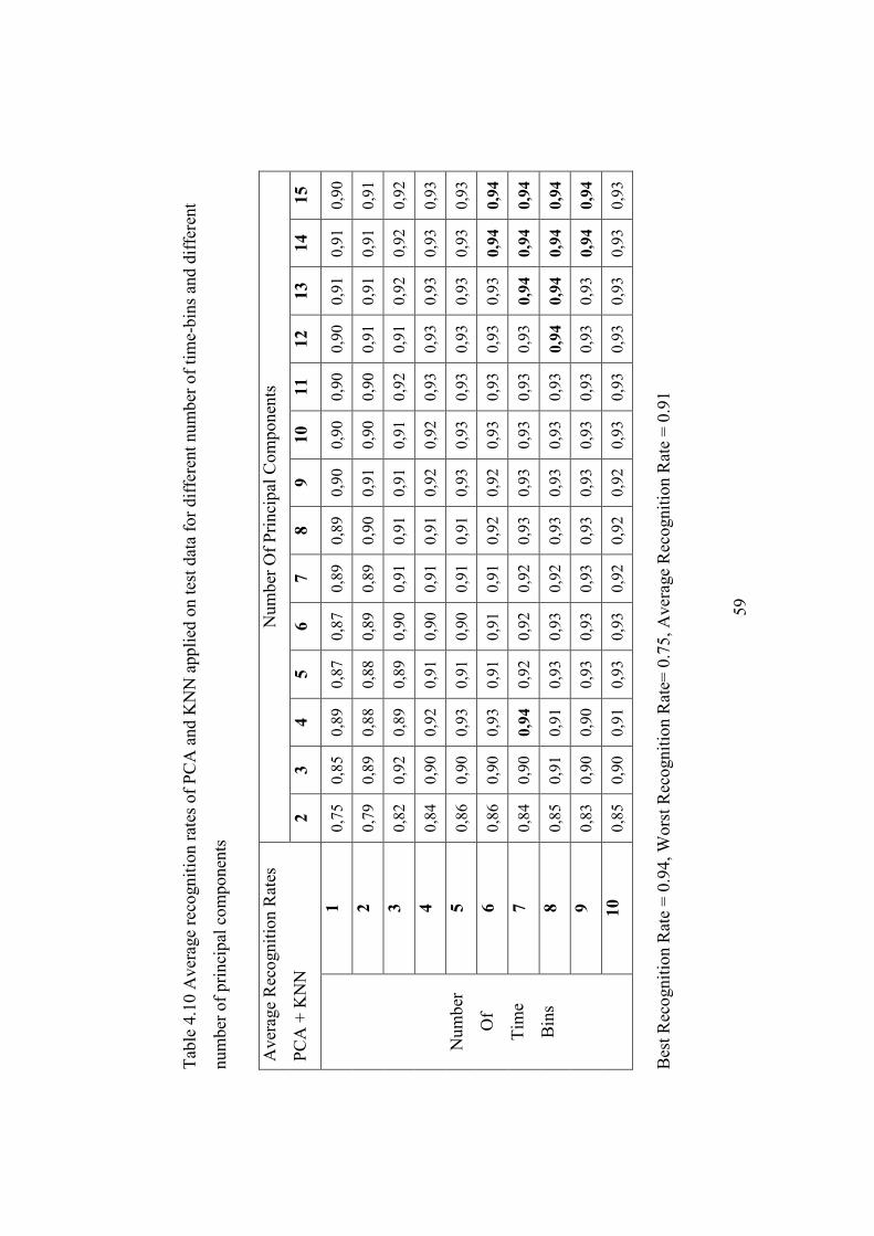
59

Tab

le 4

.10

Ave

rage

rec

ogni

tion

rat

es o

f P

CA

and

KN

N a

ppli

ed o

n te

st d

ata

for

diff

eren

t nu

mbe

r of

tim

e-bi

ns a

nd d

iffe

rent

num

ber

of p

rinc

ipal

com

pone

nts

Bes

t R

ecog

niti

on R

ate

= 0

.94,

Wor

st R

ecog

niti

on R

ate=

0.7

5, A

vera

ge R

ecog

niti

on R

ate

= 0

.91

Num

ber

Of

Pri

ncip

al C

ompo

nent

s A

vera

ge R

ecog

niti

on R

ates

PC

A +

KN

N

2 3

4 5

6 7

8 9

10

11

12

13

14

15

1 0,

75

0,85

0,

89

0,87

0,

87

0,89

0,

89

0,90

0,

90

0,90

0,

90

0,91

0,

91

0,90

2 0,

79

0,89

0,

88

0,88

0,

89

0,89

0,

90

0,91

0,

90

0,90

0,

91

0,91

0,

91

0,91

3 0,

82

0,92

0,

89

0,89

0,

90

0,91

0,

91

0,91

0,

91

0,92

0,

91

0,92

0,

92

0,92

4 0,

84

0,90

0,

92

0,91

0,

90

0,91

0,

91

0,92

0,

92

0,93

0,

93

0,93

0,

93

0,93

5 0,

86

0,90

0,

93

0,91

0,

90

0,91

0,

91

0,93

0,

93

0,93

0,

93

0,93

0,

93

0,93

6 0,

86

0,90

0,

93

0,91

0,

91

0,91

0,

92

0,92

0,

93

0,93

0,

93

0,93

0,94

0,94

7 0,

84

0,90

0,94

0,

92

0,92

0,

92

0,93

0,

93

0,93

0,

93

0,93

0,94

0,94

0,94

8 0,

85

0,91

0,

91

0,93

0,

93

0,92

0,

93

0,93

0,

93

0,93

0,94

0,94

0,94

0,94

9 0,

83

0,90

0,

90

0,93

0,

93

0,93

0,

93

0,93

0,

93

0,93

0,

93

0,93

0,94

0,94

Num

ber

Of

Tim

e

Bin

s

10

0,85

0,

90

0,91

0,

93

0,93

0,

92

0,92

0,

92

0,93

0,

93

0,93

0,

93

0,93

0,

93

60

Tab

le 4

.11

Kha

t va

lues

for

con

fusi

on m

atri

ces

of P

CA

and

SV

M a

ppli

ed o

n te

st d

ata

N

umbe

r O

f P

rinc

ipal

Com

pone

nts

Kha

t R

esul

ts

PC

A +

SV

M

2 3

4 5

6 7

8 9

10

11

12

13

14

15

1 0,

62

0,73

0,

78

0,83

0,

82

0,85

0,87

0,87

0,87

0,87

0,87

0,

86

0,86

0,

86

2 0,

64

0,81

0,

82

0,83

0,

81

0,82

0,

80

0,79

0,

79

0,79

0,

79

0,79

0,

76

0,76

3 0,

63

0,81

0,

86

0,85

0,

82

0,80

0,

78

0,75

0,

72

0,70

0,

71

0,71

0,

69

0,67

4 0,

68

0,79

0,87

0,

82

0,80

0,

75

0,71

0,

66

0,66

0,

64

0,63

0,

62

0,61

0,

61

5 0,

61

0,77

0,

84

0,78

0,

75

0,70

0,

67

0,63

0,

62

0,59

0,

58

0,56

0,

55

0,54

6 0,

61

0,71

0,

81

0,75

0,

72

0,68

0,

65

0,60

0,

57

0,55

0,

54

0,53

0,

51

0,50

7 0,

61

0,74

0,

80

0,70

0,

68

0,63

0,

61

0,56

0,

54

0,53

0,

50

0,47

0,

45

0,44

8 0,

66

0,75

0,

74

0,68

0,

63

0,61

0,

56

0,54

0,

48

0,45

0,

43

0,42

0,

41

0,38

9 0,

63

0,76

0,

69

0,68

0,

61

0,57

0,

51

0,47

0,

41

0,41

0,

39

0,37

0,

35

0,34

Num

ber

Of

Tim

e

Bin

s

10

0,53

0,

77

0,70

0,

66

0,58

0,

53

0,46

0,

38

0,35

0,

34

0,33

0,

31

0,31

0,

29

Bes

t K

hat

Val

ue =

0.8

7, W

orst

Kha

t V

alue

= 0

.29,

Ave

rage

Kha

t V

alue

= 0

.65

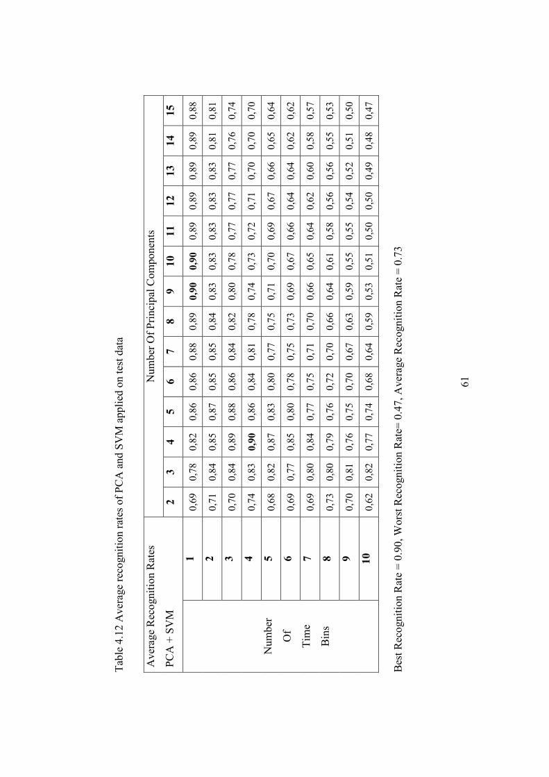
61

Tab

le 4

.12

Ave

rage

rec

ogni

tion

rat

es o

f P

CA

and

SV

M a

ppli

ed o

n te

st d

ata

N

umbe

r O

f P

rinc

ipal

Com

pone

nts

Ave

rage

Rec

ogni

tion

Rat

es

PC

A +

SV

M

2 3

4 5

6 7

8 9

10

11

12

13

14

15

1 0,

69

0,78

0,

82

0,86

0,

86

0,88

0,

89

0,90

0,90

0,

89

0,89

0,

89

0,89

0,

88

2 0,

71

0,84

0,

85

0,87

0,

85

0,85

0,

84

0,83

0,

83

0,83

0,

83

0,83

0,

81

0,81

3 0,

70

0,84

0,

89

0,88

0,

86

0,84

0,

82

0,80

0,

78

0,77

0,

77

0,77

0,

76

0,74

4 0,

74

0,83

0,90

0,

86

0,84

0,

81

0,78

0,

74

0,73

0,

72

0,71

0,

70

0,70

0,

70

5 0,

68

0,82

0,

87

0,83

0,

80

0,77

0,

75

0,71

0,

70

0,69

0,

67

0,66

0,

65

0,64

6 0,

69

0,77

0,

85

0,80

0,

78

0,75

0,

73

0,69

0,

67

0,66

0,

64

0,64

0,

62

0,62

7 0,

69

0,80

0,

84

0,77

0,

75

0,71

0,

70

0,66

0,

65

0,64

0,

62

0,60

0,

58

0,57

8 0,

73

0,80

0,

79

0,76

0,

72

0,70

0,

66

0,64

0,

61

0,58

0,

56

0,56

0,

55

0,53

9 0,

70

0,81

0,

76

0,75

0,

70

0,67

0,

63

0,59

0,

55

0,55

0,

54

0,52

0,

51

0,50

Num

ber

Of

Tim

e

Bin

s

10

0,62

0,

82

0,77

0,

74

0,68

0,

64

0,59

0,

53

0,51

0,

50

0,50

0,

49

0,48

0,

47

Bes

t R

ecog

niti

on R

ate

= 0

.90,

Wor

st R

ecog

niti

on R

ate=

0.4

7, A

vera

ge R

ecog

niti

on R

ate

= 0

.73

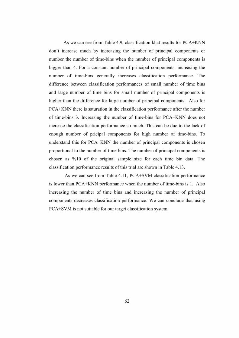
62

As we can see from Table 4.9, classification khat results for PCA+KNN

don’t increase much by increasing the number of principal components or

number the number of time-bins when the number of principal components is

bigger than 4. For a constant number of principal components, increasing the

number of time-bins generally increases classification performance. The

difference between classification performances of small number of time bins

and large number of time bins for small number of principal components is

higher than the difference for large number of principal components. Also for

PCA+KNN there is saturation in the classification performance after the number

of time-bins 3. Increasing the number of time-bins for PCA+KNN does not

increase the classification performance so much. This can be due to the lack of

enough number of pricipal components for high number of time-bins. To

understand this for PCA+KNN the number of principal components is chosen

proportional to the number of time bins. The number of principal components is

chosen as %10 of the original sample size for each time bin data. The

classification performance results of this trial are shown in Table 4.13.

As we can see from Table 4.11, PCA+SVM classification performance

is lower than PCA+KNN performance when the number of time-bins is 1. Also

increasing the number of time bins and increasing the number of principal

components decreases classification performance. We can conclude that using

PCA+SVM is not suitable for our target classification system.

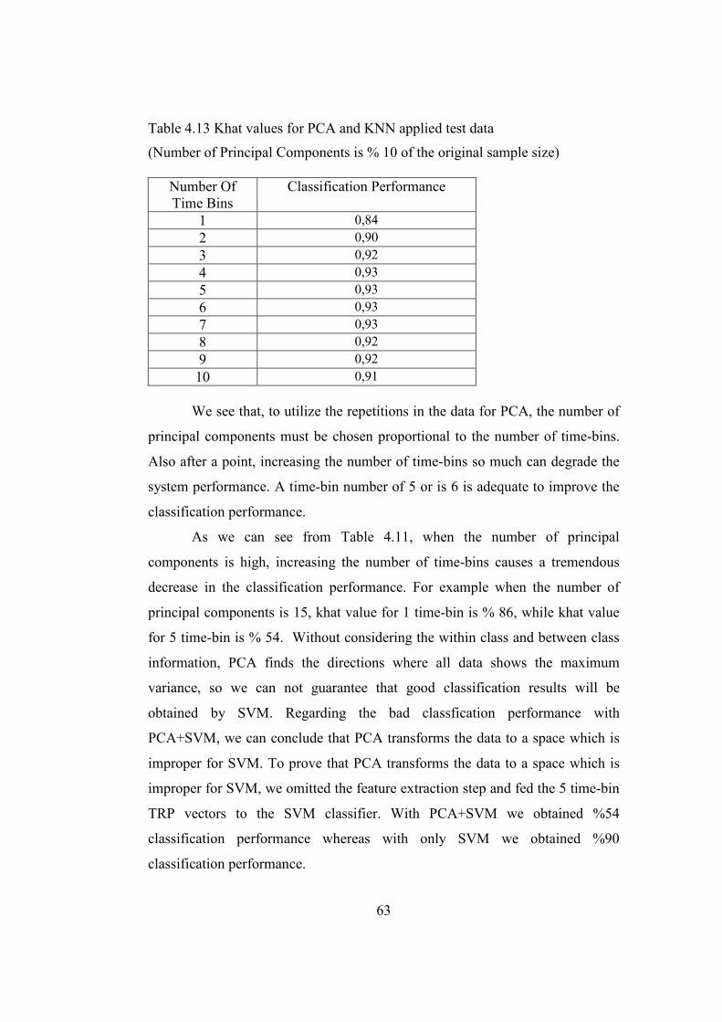
63

Table 4.13 Khat values for PCA and KNN applied test data

(Number of Principal Components is % 10 of the original sample size)

Number Of Time Bins

Classification Performance

1 0,84

2 0,90

3 0,92

4 0,93

5 0,93

6 0,93

7 0,93

8 0,92

9 0,92

10 0,91

We see that, to utilize the repetitions in the data for PCA, the number of

principal components must be chosen proportional to the number of time-bins.

Also after a point, increasing the number of time-bins so much can degrade the

system performance. A time-bin number of 5 or is 6 is adequate to improve the


As we can see from Table 4.11, when the number of principal

components is high, increasing the number of time-bins causes a tremendous

decrease in the classification performance. For example when the number of

principal components is 15, khat value for 1 time-bin is % 86, while khat value

for 5 time-bin is % 54. Without considering the within class and between class

information, PCA finds the directions where all data shows the maximum

variance, so we can not guarantee that good classification results will be

obtained by SVM. Regarding the bad classfication performance with

PCA+SVM, we can conclude that PCA transforms the data to a space which is

improper for SVM. To prove that PCA transforms the data to a space which is

improper for SVM, we omitted the feature extraction step and fed the 5 time-bin

TRP vectors to the SVM classifier. With PCA+SVM we obtained %54

classification performance whereas with only SVM we obtained %90


64

Tab

le 4

.14

Kha

t va

lues

of

LD

A a

nd K

NN

app

lied

on

test

dat

a

N

umbe

r O

f P

rinc

ipal

Com

pone

nts

Kha

t R

esul

ts

LD

A +

KN

N

2 3

4 5

6 7

8 9

10

11

12

13

14

15

1 0,

53

0,71

0,

79

0,78

0,

80

0,79

0,

79

0,80

0,

79

0,78

0,

79

0,80

0,

81

0,81

2 0,

67

0,73

0,

79

0,76

0,

83

0,84

0,

84

0,85

0,

86

0,85

0,

85

0,85

0,

85

0,85

3 0,

76

0,77

0,

80

0,76

0,

83

0,84

0,

84

0,85

0,

85

0,85

0,

84

0,84

0,

84

0,85

4 0,

67

0,75

0,

76

0,82

0,

87

0,87

0,

87

0,87

0,

86

0,86

0,

86

0,87

0,

87

0,86

5 0,

60

0,70

0,

79

0,82

0,

89

0,89

0,

89

0,90

0,

90

0,90

0,

90

0,90

0,

91

0,90

6 0,

67

0,74

0,

84

0,86

0,

92

0,91

0,

91

0,91

0,

91

0,91

0,

92

0,92

0,

92

0,92

7 0,

63

0,77

0,

82

0,87

0,

93

0,92

0,

92

0,93

0,

93

0,93

0,

93

0,93

0,

93

0,93

8 0,

76

0,82

0,

85

0,91

0,

92

0,92

0,

92

0,92

0,

92

0,92

0,

92

0,92

0,

92

0,92

9 0,

78

0,84

0,

87

0,92

0,

93

0,93

0,

92

0,93

0,

93

0,93

0,

92

0,93

0,

92

0,92

Num

ber

Of

Tim

e

Bin

s

10

0,81

0,

87

0,89

0,

93

0,93

0,

93

0,93

0,

93

0,93

0,

93

0,93

0,

93

0,94

0,

93

Bes

t K

hat

Val

ue =

0.9

4, W

orst

Kha

t V

alue

= 0

.53,

Ave

rage

Kha

t V

alue

= 0

.86

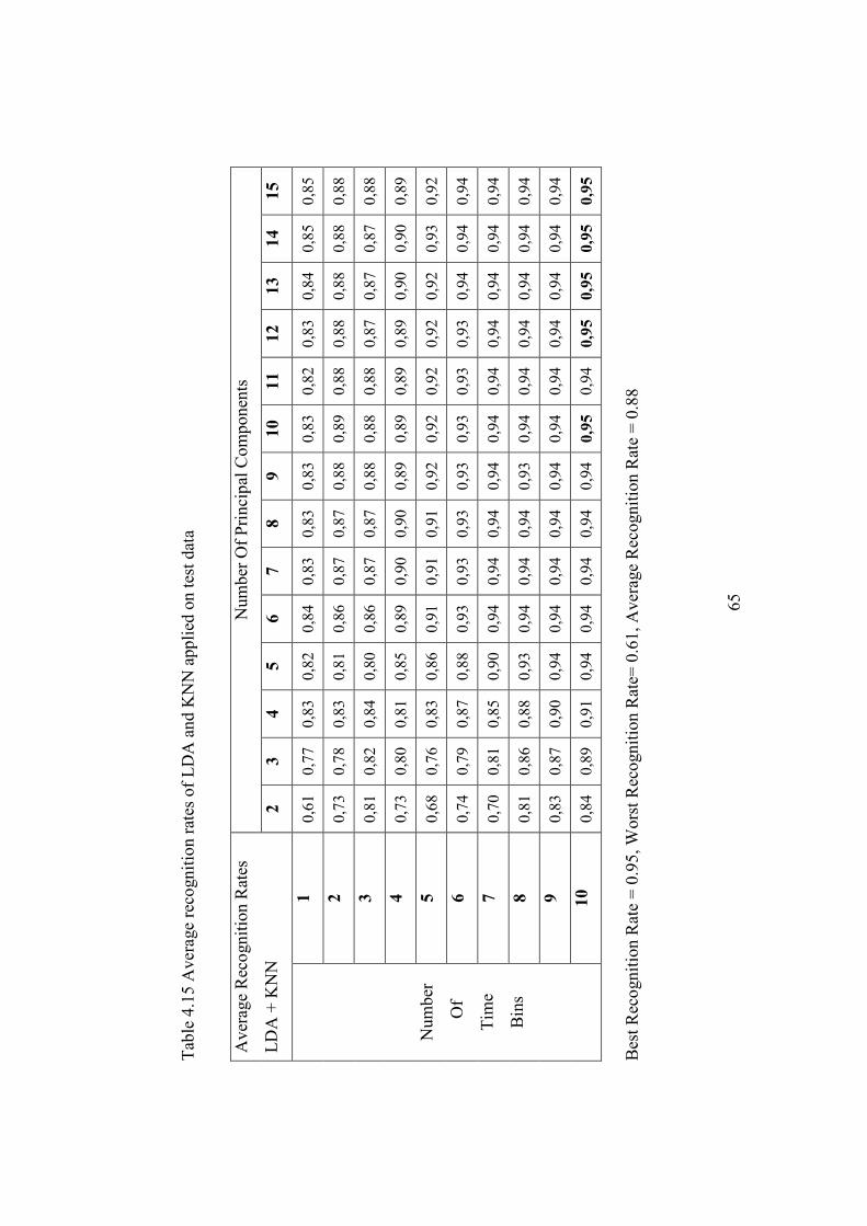
65

Tab

le 4

.15

Ave

rage

rec

ogni

tion

rat

es o

f L

DA

and

KN

N a

ppli

ed o

n te

st d

ata

Bes

t R

ecog

niti

on R

ate

= 0

.95,

Wor

st R

ecog

niti

on R

ate=

0.6

1, A

vera

ge R

ecog

niti

on R

ate

= 0

.88

Num

ber

Of

Pri

ncip

al C

ompo

nent

s A

vera

ge R

ecog

niti

on R

ates

LD

A +

KN

N

2 3

4 5

6 7

8 9

10

11

12

13

14

15

1 0,

61

0,77

0,

83

0,82

0,

84

0,83

0,

83

0,83

0,

83

0,82

0,

83

0,84

0,

85

0,85

2 0,

73

0,78

0,

83

0,81

0,

86

0,87

0,

87

0,88

0,

89

0,88

0,

88

0,88

0,

88

0,88

3 0,

81

0,82

0,

84

0,80

0,

86

0,87

0,

87

0,88

0,

88

0,88

0,

87

0,87

0,

87

0,88

4 0,

73

0,80

0,

81

0,85

0,

89

0,90

0,

90

0,89

0,

89

0,89

0,

89

0,90

0,

90

0,89

5 0,

68

0,76

0,

83

0,86

0,

91

0,91

0,

91

0,92

0,

92

0,92

0,

92

0,92

0,

93

0,92

6 0,

74

0,79

0,

87

0,88

0,

93

0,93

0,

93

0,93

0,

93

0,93

0,

93

0,94

0,

94

0,94

7 0,

70

0,81

0,

85

0,90

0,

94

0,94

0,

94

0,94

0,

94

0,94

0,

94

0,94

0,

94

0,94

8 0,

81

0,86

0,

88

0,93

0,

94

0,94

0,

94

0,93

0,

94

0,94

0,

94

0,94

0,

94

0,94

9 0,

83

0,87

0,

90

0,94

0,

94

0,94

0,

94

0,94

0,

94

0,94

0,

94

0,94

0,

94

0,94

Num

ber

O

f

Tim

e

Bin

s

10

0,84

0,

89

0,91

0,

94

0,94

0,

94

0,94

0,

94

0,95

0,

94

0,95

0,95

0,95

0,95

66

Tab

le 4

.16

Kha

t va

lues

of

LD

A a

nd S

VM

app

lied

on

test

dat

a

Num

ber

Of

Pri

ncip

al C

ompo

nent

s K

hat

Res

ults

LD

A +

SV

M

2 3

4 5

6 7

8 9

10

11

12

13

14

15

1 0,

52

0,57

0,

61

0,61

0,

71

0,68

0,

65

0,65

0,

69

0,67

0,

70

0,72

0,

76

0,75

2 0,

68

0,66

0,

71

0,67

0,

78

0,77

0,

80

0,76

0,

81

0,81

0,

82

0,82

0,

83

0,83

3 0,

74

0,70

0,

75

0,73

0,

73

0,75

0,

83

0,85

0,

82

0,83

0,

83

0,88

0,

86

0,88

4 0,

63

0,71

0,

60

0,83

0,

80

0,81

0,

81

0,85

0,

87

0,83

0,

82

0,86

0,

87

0,88

5 0,

62

0,67

0,

75

0,87

0,

92

0,89

0,

87

0,87

0,

89

0,89

0,

92

0,91

0,

92

0,92

6 0,

65

0,62

0,

76

0,89

0,

89

0,91

0,

90

0,91

0,

90

0,91

0,

91

0,93

0,

92

0,93

7 0,

61

0,79

0,

75

0,96

0,

95

0,96

0,

96

0,93

0,

93

0,94

0,

95

0,96

0,

96

0,96

8 0,

72

0,73

0,

78

0,93

0,

99

0,95

0,

95

0,94

0,

94

0,96

0,

97

0,97

0,

96

0,96

9 0,

69

0,78

0,

69

0,93

0,

93

0,94

0,

95

0,97

0,

97

0,96

0,98

0,98

0,98

0,98

Num

ber

Of

Tim

e

Bin

s

10

0,71

0,

78

0,87

0,

96

0,96

0,

93

0,95

0,

94

0,96

0,

96

0,96

0,

96

0,96

0,

96

Bes

t K

hat

Val

ue =

0.9

8, W

orst

Kha

t V

alue

= 0

.52,

Ave

rage

Kha

t V

alue

= 0

.84

67

Tab

le 4

.17

Ave

rage

rec

ogni

tion

rat

es o

f L

DA

and

SV

M a

ppli

ed o

n te

st d

ata

Bes

t R

ecog

niti

on R

ate

= 0

.98,

Wor

st R

ecog

niti

on R

ate=

0.6

1, A

vera

ge R

ecog

niti

on R

ate

= 0

.87

Num

ber

Of

Pri

ncip

al C

ompo

nent

s A

vera

ge R

ecog

niti

on R

ates

LD

A +

SV

M

2 3

4 5

6 7

8 9

10

11

12

13

14

15

1 0,

61

0,64

0,

68

0,69

0,

76

0,74

0,

71

0,72

0,

75

0,74

0,

76

0,77

0,

81

0,80

2 0,

74

0,72

0,

76

0,74

0,

83

0,81

0,

84

0,81

0,

84

0,84

0,

86

0,86

0,

86

0,86

3 0,

79

0,76

0,

80

0,78

0,

78

0,80

0,

86

0,88

0,

86

0,86

0,

86

0,90

0,

89

0,90

4 0,

70

0,77

0,

68

0,86

0,

83

0,85

0,

85

0,88

0,

90

0,86

0,

86

0,89

0,

90

0,90

5 0,

70

0,73

0,

80

0,90

0,

93

0,91

0,

89

0,89

0,

91

0,92

0,

93

0,93

0,

94

0,93

6 0,

71

0,69

0,

81

0,91

0,

91

0,93

0,

92

0,93

0,

92

0,93

0,

93

0,94

0,

94

0,94

7 0,

69

0,83

0,

80

0,97

0,

96

0,97

0,

97

0,94

0,

95

0,95

0,

96

0,97

0,

97

0,96

8 0,

77

0,78

0,

83

0,95

0,

99

0,96

0,

96

0,95

0,

95

0,97

0,

97

0,97

0,

97

0,97

9 0,

75

0,82

0,

75

0,94

0,

94

0,95

0,

96

0,97

0,

97

0,97

0,98

0,98

0,98

0,98

Num

ber

Of

Tim

e

Bin

s

10

0,77

0,

82

0,90

0,

97

0,97

0,

95

0,96

0,

96

0,97

0,

97

0,97

0,

97

0,97

0,

97

68

As we can see from Table 4.14, increasing the number of time bins for

LDA + KNN causes a tremendous change in the classsification performance.

When the number of principal components is 2, the classification performance is

% 53 for 1 time-bin data and classification performance is % 81 for 10 time-bin

data. When the number of principal components is 15, classification

performance is %81 for 1 time-bin data and classification performance is %93

for 10 time-bin data. Even a classification performance improvement of %12 is

obtained for large number of principal components by increasing the number of

time bins.

As we can see from Table 4.16, increasing the number of time-bins for

LDA+SVM also causes a tremendous change in the classification performance.

When the number of principal components is 2, the classification performances

for 1 time-bin data and for 10 time-bin data are %52 and %71. When the

number of principal components is 15, the classifications performances for 1

time-bin data and 10 time-bin data are %75 and %96 respectively. The

maximum classification performance obtained with LDA+SVM is %98 which

outperforms PCA+KNN. PCA+KNN classification performance is better for

small number of principal components and small number of time bins than

LDA+SVM, however LDA+SVM classification performance is much better

than PCA+KNN for large number of principal components and large number of

time bins.

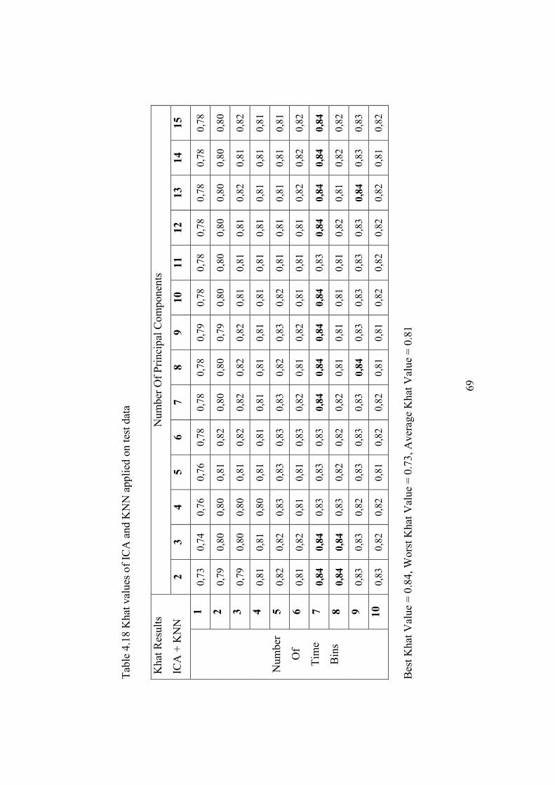
69

Tab

le 4

.18

Kha

t va

lues

of

ICA

and

KN

N a

ppli

ed o

n te

st d

ata

N

umbe

r O

f P

rinc

ipal

Com

pone

nts

Kha

t R

esul

ts

ICA

+ K

NN

2

3 4

5 6

7 8

9 10

11

12

13

14

15

1 0,

73

0,74

0,

76

0,76

0,

78

0,78

0,

78

0,79

0,

78

0,78

0,

78

0,78

0,

78

0,78

2 0,

79

0,80

0,

80

0,81

0,

82

0,80

0,

80

0,79

0,

80

0,80

0,

80

0,80

0,

80

0,80

3 0,

79

0,80

0,

80

0,81

0,

82

0,82

0,

82

0,82

0,

81

0,81

0,

81

0,82

0,

81

0,82

4 0,

81

0,81

0,

80

0,81

0,

81

0,81

0,

81

0,81

0,

81

0,81

0,

81

0,81

0,

81

0,81

5 0,

82

0,82

0,

83

0,83

0,

83

0,83

0,

82

0,83

0,

82

0,81

0,

81

0,81

0,

81

0,81

6 0,

81

0,82

0,

81

0,81

0,

83

0,82

0,

81

0,82

0,

81

0,81

0,

81

0,82

0,

82

0,82

7 0,84

0,84

0,

83

0,83

0,

83

0,84

0,84

0,84

0,84

0,

83

0,84

0,84

0,84

0,84

8 0,84

0,84

0,

83

0,82

0,

82

0,82

0,

81

0,81

0,

81

0,81

0,

82

0,81

0,

82

0,82

9 0,

83

0,83

0,

82

0,83

0,

83

0,83

0,84

0,

83

0,83

0,

83

0,83

0,84

0,

83

0,83

Num

ber

Of

Tim

e

Bin

s

10

0,83

0,

82

0,82

0,

81

0,82

0,

82

0,81

0,

81

0,82

0,

82

0,82

0,

82

0,81

0,

82

Bes

t K

hat

Val

ue =

0.8

4, W

orst

Kha

t V

alue

= 0

.73,

Ave

rage

Kha

t V

alue

= 0

.81

70

Tab

le 4

.19

Ave

rage

rec

ogni

tion

rat

es o

f IC

A a

nd K

NN

app

lied

on

test

dat

a

Bes

t R

ecog

niti

on R

ate

= 0

.87,

Wor

st R

ecog

niti

on R

ate=

0.7

8, A

vera

ge R

ecog

niti

on R

ate

= 0

.85

Num

ber

Of

Pri

ncip

al C

ompo

nent

s A

vera

ge R

ecog

niti

on R

ates

ICA

+ K

NN

2

3 4

5 6

7 8

9 10

11

12

13

14

15

1 0,

78

0,79

0,

80

0,80

0,

82

0,82

0,

82

0,83

0,

82

0,82

0,

82

0,82

0,

82

0,82

2 0,

83

0,84

0,

84

0,85

0,

85

0,84

0,

84

0,83

0,

83

0,84

0,

84

0,84

0,

84

0,84

3 0,

83

0,84

0,

84

0,85

0,

85

0,85

0,

85

0,85

0,

85

0,85

0,

85

0,85

0,

85

0,85

4 0,

84

0,85

0,

84

0,85

0,

85

0,85

0,

85

0,85

0,

85

0,85

0,

85

0,85

0,

85

0,85

5 0,

86

0,85

0,

86

0,87

0,87

0,

86

0,86

0,

86

0,86

0,

85

0,85

0,

85

0,85

0,

85

6 0,

85

0,85

0,

85

0,85

0,

86

0,86

0,

85

0,85

0,

85

0,85

0,

85

0,85

0,

85

0,85

7 0,87

0,87

0,

86

0,86

0,87

0,87

0,87

0,87

0,87

0,

86

0,87

0,87

0,87

0,87

8 0,87

0,87

0,

86

0,86

0,

85

0,86

0,

85

0,85

0,

85

0,85

0,

86

0,85

0,

85

0,86

9 0,87

0,

86

0,86

0,

86

0,86

0,

86

0,87

0,87

0,87

0,87

0,87

0,87

0,87

0,87

Num

ber

Of

Tim

e

Bin

s

10

0,86

0,

86

0,85

0,

85

0,85

0,

85

0,85

0,

85

0,85

0,

85

0,86

0,

85

0,85

0,

86

71

Tab

le 4

.20

Kha

t va

lues

of

ICA

and

SV

M a

ppli

ed o

n te

st d

ata

N

umbe

r O

f P

rinc

ipal

Com

pone

nts

Kha

t R

esul

ts

ICA

+ S

VM

2

3 4

5 6

7 8

9 10

11

12

13

14

15

1 0,

79

0,79

0,

82

0,82

0,

84

0,85

0,

85

0,83

0,

83

0,83

0,

82

0,83

0,

83

0,84

2 0,

79

0,81

0,

81

0,85

0,

85

0,87

0,

87

0,88

0,

88

0,87

0,

87

0,87

0,

86

0,86

3 0,

82

0,81

0,

81

0,85

0,

86

0,87

0,

88

0,89

0,

88

0,88

0,

88

0,89

0,

89

0,89

4 0,

84

0,84

0,

83

0,87

0,

88

0,89

0,

90

0,90

0,

89

0,88

0,

89

0,89

0,

88

0,88

5 0,

84

0,85

0,

86

0,88

0,

87

0,87

0,

88

0,88

0,

88

0,87

0,

87

0,88

0,

86

0,88

6 0,

82

0,82

0,

83

0,83

0,

84

0,84

0,

84

0,87

0,

87

0,88

0,

89

0,89

0,

89

0,88

7 0,

82

0,80

0,

81

0,85

0,

92

0,91

0,

90

0,89

0,

86

0,87

0,

90

0,89

0,

90

0,90

8 0,

81

0,82

0,

82

0,82

0,

86

0,89

0,

89

0,88

0,

91

0,90

0,

92

0,93

0,

92

0,93

9 0,

83

0,82

0,

82

0,80

0,

81

0,86

0,

85

0,89

0,

88

0,91

0,

92

0,93

0,

92

0,94

Num

ber

Of

Tim

e

Bin

s

10

0,83

0,

82

0,82

0,

80

0,83

0,

88

0,89

0,

90

0,94

0,

94

0,94

0,

94

0,96

0,97

Bes

t K

hat

Val

ue =

0.9

7, W

orst

Kha

t V

alue

= 0

.79,

Ave

rage

Kha

t V

alue

= 0

.87

72

Tab

le 4

.21

Ave

rage

rec

ogni

tion

rat

es o

f IC

A a

nd S

VM

app

lied

on

test

dat

a

N

umbe

r O

f P

rinc

ipal

Com

pone

nts

Ave

rage

Rec

ogni

tion

Rat

es

ICA

+ S

VM

2

3 4

5 6

7 8

9 10

11

12

13

14

15

1 0,

83

0,83

0,

86

0,86

0,

87

0,88

0,

88

0,86

0,

86

0,86

0,

86

0,86

0,

86

0,87

2 0,

83

0,85

0,

85

0,87

0,

88

0,89

0,

90

0,90

0,

90

0,90

0,

89

0,89

0,

89

0,89

3 0,

85

0,85

0,

85

0,88

0,

89

0,89

0,

90

0,91

0,

91

0,90

0,

90

0,91

0,

91

0,91

4 0,

87

0,87

0,

86

0,90

0,

90

0,91

0,

92

0,92

0,

91

0,91

0,

91

0,91

0,

90

0,90

5 0,

87

0,88

0,

88

0,90

0,

90

0,89

0,

90

0,91

0,

90

0,90

0,

90

0,90

0,

89

0,90

6 0,

86

0,85

0,

86

0,87

0,

87

0,87

0,

87

0,90

0,

90

0,91

0,

91

0,91

0,

91

0,90

7 0,

86

0,84

0,

84

0,88

0,

94

0,93

0,

92

0,91

0,

89

0,90

0,

92

0,91

0,

92

0,92

8 0,

85

0,86

0,

86

0,86

0,

89

0,91

0,

91

0,90

0,

93

0,92

0,

93

0,94

0,

93

0,95

9 0,

87

0,86

0,

86

0,84

0,

85

0,89

0,

88

0,91

0,

91

0,93

0,

94

0,94

0,

94

0,95

Num

ber

Of

Tim

e

Bin

s

10

0,86

0,

86

0,86

0,

84

0,86

0,

91

0,91

0,

92

0,95

0,

95

0,96

0,

95

0,97

0,97

Bes

t R

ecog

niti

on R

ate

= 0

.97,

Wor

st R

ecog

niti

on R

ate=

0.8

3, A

vera

ge R

ecog

niti

on R

ate

= 0

.89

73

As we can see from Table 4.18, for constant number of time bins the

classification performance of ICA+KNN does not change much by increasing

the number of principal components. When the number of principal components

is constant, a classification performance improvement of % 4 to % 10 is

obtained for different number of principal components. The classification

performance of ICA+KNN is satisfactory but could not compete with the

classification performance of LDA+SVM or LDA+KNN.

As we can see from the Table 4.20, the minimum classification

performance of ICA+SVM is %79. ICA+SVM outperforms LDA+SVM,

LDA+KNN and PCA+KNN in minimum classification performance.

Comparing to ICA+KNN, increasing the number of principal components

improves classification performance of ICA+SVM tremendously. When the

number of principal components is 2, the classification performances for 1 time-

bin data and 10 time-bin data are %79 and %83 respectively. When the number

of principal components is 15, the classification performances for 1 time-bin

data and 10 time-bin data are %84 and %97 respectively. The maximum

classification performance obtained with ICA+SVM is %97 which is very close

to the maximum classification performance of LDA+SVM of %98. Regarding

that the classification performance of LDA+SVM is not satisfactory enough for

small numbers of principal components and small number of time bins, we can

conclude that using ICA in the feature extraction stage and using SVM in the

classifier stage is the best choice for our target recognition system.

74

Tab

le 4

.22

Kha

t va

lues

of

NM

F a

nd K

NN

app

lied

on

test

dat

a

N

umbe

r O

f P

rinc

ipal

Com

pone

nts

Kha

t R

esul

ts

NM

F +

KN

N

2 3

4 5

6 7

8 9

10

11

12

13

14

15

1 0,

21

0,35

0,

55

0,59

0,

61

0,67

0,

71

0,71

0,

74

0,77

0,

76

0,78

0,

80

0,81

2 0,

29

0,45

0,

57

0,63

0,

69

0,72

0,

72

0,79

0,

76

0,78

0,

82

0,85

0,

85

0,86

3 0,

39

0,42

0,

48

0,68

0,

65

0,72

0,

77

0,76

0,

83

0,80

0,

86

0,85

0,

86

0,87

4 0,

33

0,43

0,

54

0,57

0,

66

0,75

0,

79

0,82

0,

83

0,81

0,

84

0,87

0,

87

0,87

5 0,

42

0,41

0,

69

0,64

0,

65

0,78

0,

80

0,81

0,

86

0,82

0,

87

0,87

0,

86

0,89

6 0,

46

0,50

0,

62

0,66

0,

61

0,76

0,

79

0,81

0,

85

0,84

0,

85

0,86

0,

86

0,88

7 0,

47

0,45

0,

50

0,69

0,

61

0,76

0,

78

0,80

0,

84

0,86

0,

85

0,87

0,89

0,89

8 0,

36

0,46

0,

56

0,59

0,

75

0,73

0,

76

0,78

0,

82

0,87

0,

87

0,86

0,

88

0,88

9 0,

30

0,56

0,

57

0,61

0,

75

0,74

0,

81

0,83

0,

83

0,84

0,

86

0,87

0,

88

0,88

Num

ber

Of

Tim

e

Bin

s

10

0,49

0,

52

0,55

0,

70

0,73

0,

72

0,82

0,

83

0,82

0,

84

0,86

0,

85

0,88

0,

88

Bes

t K

hat

Val

ue =

0.8

9, W

orst

Kha

t V

alue

= 0

.21,

Ave

rage

Kha

t V

alue

= 0

.72

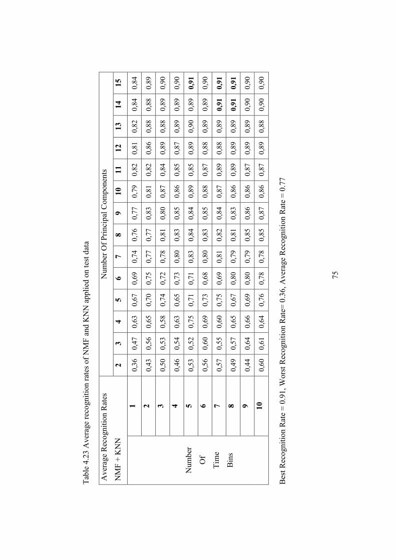
75

Tab

le 4

.23

Ave

rage

rec

ogni

tion

rat

es o

f N

MF

and

KN

N a

ppli

ed o

n te

st d

ata

Num

ber

Of

Pri

ncip

al C

ompo

nent

s A

vera

ge R

ecog

niti

on R

ates

NM

F +

KN

N

2 3

4 5

6 7

8 9

10

11

12

13

14

15

1 0,

36

0,47

0,

63

0,67

0,

69

0,74

0,

76

0,77

0,

79

0,82

0,

81

0,82

0,

84

0,84

2 0,

43

0,56

0,

65

0,70

0,

75

0,77

0,

77

0,83

0,

81

0,82

0,

86

0,88

0,

88

0,89

3 0,

50

0,53

0,

58

0,74

0,

72

0,78

0,

81

0,80

0,

87

0,84

0,

89

0,88

0,

89

0,90

4 0,

46

0,54

0,

63

0,65

0,

73

0,80

0,

83

0,85

0,

86

0,85

0,

87

0,89

0,

89

0,90

5 0,

53

0,52

0,

75

0,71

0,

71

0,83

0,

84

0,84

0,

89

0,85

0,

89

0,90

0,

89

0,91

6 0,

56

0,60

0,

69

0,73

0,

68

0,80

0,

83

0,85

0,

88

0,87

0,

88

0,89

0,

89

0,90

7 0,

57

0,55

0,

60

0,75

0,

69

0,81

0,

82

0,84

0,

87

0,89

0,

88

0,89

0,91

0,91

8 0,

49

0,57

0,

65

0,67

0,

80

0,79

0,

81

0,83

0,

86

0,89

0,

89

0,89

0,91

0,91

9 0,

44

0,64

0,

66

0,69

0,

80

0,79

0,

85

0,86

0,

86

0,87

0,

89

0,89

0,

90

0,90

Num

ber

Of

Tim

e

Bin

s

10

0,60

0,

61

0,64

0,

76

0,78

0,

78

0,85

0,

87

0,86

0,

87

0,89

0,

88

0,90

0,

90

Bes

t R

ecog

niti

on R

ate

= 0

.91,

Wor

st R

ecog

niti

on R

ate=

0.3

6, A

vera

ge R

ecog

niti

on R

ate

= 0

.77

76

Tab

le 4

.24

Kha

t va

lues

of

NM

F a

nd S

VM

app

lied

on

test

dat

a

N

umbe

r O

f P

rinc

ipal

Com

pone

nts

Kha

t R

esul

ts

NM

F +

SV

M

2 3

4 5

6 7

8 9

10

11

12

13

14

15

1 0,

33

0,40

0,

59

0,59

0,

62

0,69

0,

69

0,73

0,

77

0,75

0,

77

0,79

0,

79

0,80

2 0,

38

0,49

0,

62

0,63

0,

70

0,70

0,

73

0,78

0,

77

0,78

0,

83

0,87

0,

88

0,89

3 0,

41

0,49

0,

54

0,65

0,

68

0,70

0,

75

0,76

0,

84

0,81

0,

85

0,88

0,

89

0,89

4 0,

39

0,48

0,

53

0,64

0,

68

0,72

0,

78

0,80

0,

84

0,85

0,

84

0,88

0,

89

0,90

5 0,

43

0,48

0,

64

0,66

0,

68

0,76

0,

79

0,83

0,

84

0,85

0,

88

0,92

0,

91

0,93

6 0,

43

0,50

0,

64

0,66

0,

65

0,70

0,

81

0,80

0,

86

0,87

0,

89

0,92

0,

93

0,92

7 0,

45

0,53

0,

58

0,69

0,

67

0,76

0,

81

0,81

0,

85

0,85

0,

87

0,91

0,

92

0,93

8 0,

41

0,47

0,

61

0,60

0,

67

0,71

0,

75

0,77

0,

83

0,88

0,

90

0,91

0,

91

0,93

9 0,

36

0,55

0,

59

0,59

0,

72

0,72

0,

79

0,84

0,

85

0,87

0,

90

0,92

0,

94

0,97

Num

ber

Of

Tim

e

Bin

s

10

0,52

0,

53

0,54

0,

66

0,71

0,

78

0,81

0,

85

0,83

0,

86

0,90

0,

92

0,94

0,

95

Bes

t K

hat

Val

ue =

0.9

7, W

orst

Kha

t V

alue

= 0

.33,

Ave

rage

Kha

t V

alue

= 0

.74

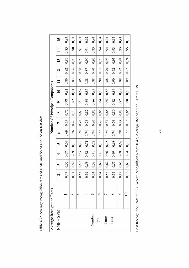
77

Tab

le 4

.25

Ave

rage

rec

ogni

tion

rat

es o

f N

MF

and

SV

M a

ppli

ed o

n te

st d

ata

N

umbe

r O

f P

rinc

ipal

Com

pone

nts

Ave

rage

Rec

ogni

tion

Rat

es

NM

F +

SV

M

2 3

4 5

6 7

8 9

10

11

12

13

14

15

1 0,

47

0,52

0,

67

0,67

0,

69

0,75

0,

75

0,78

0,

81

0,80

0,

82

0,83

0,

83

0,84

2 0,

51

0,59

0,

69

0,70

0,

76

0,76

0,

78

0,82

0,

81

0,83

0,

86

0,90

0,

90

0,91

3 0,

53

0,59

0,

63

0,72

0,

74

0,76

0,

80

0,81

0,

87

0,85

0,

88

0,90

0,

91

0,91

4 0,

51

0,58

0,

62

0,71

0,

74

0,78

0,

82

0,84

0,

87

0,88

0,

87

0,90

0,

91

0,92

5 0,

54

0,58

0,

71

0,72

0,

74

0,80

0,

83

0,86

0,

87

0,88

0,

90

0,93

0,

93

0,94

6 0,

54

0,60

0,

71

0,73

0,

72

0,76

0,

85

0,84

0,

88

0,90

0,

91

0,93

0,

94

0,94

7 0,

56

0,62

0,

66

0,75

0,

74

0,81

0,

85

0,85

0,

88

0,88

0,

90

0,93

0,

94

0,94

8 0,

54

0,57

0,

69

0,68

0,

74

0,76

0,

80

0,82

0,

86

0,90

0,

92

0,93

0,

93

0,95

9 0,

49

0,65

0,

68

0,68

0,

78

0,78

0,

83

0,87

0,

88

0,89

0,

92

0,94

0,

95

0,97

Num

ber

Of

Tim

e

Bin

s

10

0,62

0,

63

0,64

0,

73

0,77

0,

82

0,85

0,

88

0,86

0,

89

0,92

0,

94

0,95

0,

96

Bes

t R

ecog

niti

on R

ate

= 0

.97,

Wor

st R

ecog

niti

on R

ate=

0.4

7, A

vera

ge R

ecog

niti

on R

ate

= 0

.79

78

As we can see from Table 4.22 NMF+KNN does not provide us good

classification performance results for small numbers of principal components.

The number of principal components must be at least 5 to get a classification

performance of %70.

As we can see from Table 4.24, the classification performance of

NMF+SVM is better than classification performance of NMF+KNN. Like

NMF+KNN, NMF+SVM provides poor classification performance for small

number of time bins and small number of principal components. However, for

large values of principal components and time bins NMF+SVM provides good

performance. The maximum classification performance obtained with

NMF+SVM is %97. The classification performances of NMF+KNN and

NMF+SVM can be considered as the worst classification performances among

the feature extraction algoritms applied.

We can conclude that NMF is not good at extracting the significant

features of data. With ICA+SVM the classification performance is %79 with a

principal component value of 2 and time bin value of 1, however with

NMF+SVM the classification performance value is only %33 with the same

number of principal components and number of time-bins. Regarding Table

4.22, when the number of time bins 1, the classification performance increases

from %21 to %81 with the increase of the number of principal components from

2 to 15.

Despite taking average of 10 experiments with different random initial

values for NMF, there are some cases for which reliable classification

performance results can not be obtained. In Table 4.22, when the number of

principal components is 5, increasing the number of time bins can cause

fluctuations. For example khat value for 3 time-bins is %68, while khat value for

4 time-bins is %57. Also khat value for 9 time-bins is %61 and khat value for 10

time-bins is %70. This is due to the fact that NMF can give different results for

different iterations.

79

4.3 Hierarchical Classification Performance Results In this section the classification performance results for the hierarchical

target recognition system shown in Figure 3.8 are presented. Classification

performance results calculated are KHAT (2.11) and Average Recognition Rate

(2.12). Classification performance results are calculated for various numbers of

time-bins and various numbers of principal components. These results are

presented through Table 4.26 to Table 4.41.

80

Tab

le 4

.26

Kha

t va

lues

of

PC

A a

nd K

NN

app

lied

on

test

dat

a

Bes

t K

hat

Val

ue =

0.9

4, W

orst

Kha

t V

alue

= 0

.76,

Ave

rage

Kha

t V

alue

= 0

.90

Num

ber

Of

Pri

ncip

al C

ompo

nent

s K

hat

Res

ults

Hie

rarc

hica

l

PC

A +

KN

N

2 3

4 5

6 7

8 9

10

11

12

13

14

15

1 0,

76

0,82

0,

86

0,87

0,

86

0,89

0,

89

0,90

0,

89

0,88

0,

90

0,89

0,

89

0,89

2 0,

79

0,84

0,

87

0,89

0,

90

0,90

0,

90

0,90

0,

90

0,90

0,

90

0,90

0,

90

0,90

3 0,

79

0,86

0,

87

0,90

0,

91

0,91

0,

90

0,93

0,

92

0,91

0,

92

0,92

0,

93

0,92

4 0,

78

0,85

0,

87

0,87

0,

91

0,91

0,

91

0,92

0,94

0,

93

0,94

0,94

0,94

0,94

5 0,

77

0,86

0,

88

0,88

0,

92

0,92

0,

92

0,91

0,

92

0,93

0,

92

0,93

0,

93

0,93

6 0,

81

0,81

0,

87

0,87

0,

89

0,91

0,

91

0,91

0,

91

0,92

0,

92

0,93

0,

93

0,94

7 0,

83

0,82

0,

87

0,89

0,

89

0,93

0,

93

0,93

0,

92

0,93

0,94

0,

93

0,93

0,

93

8 0,

83

0,82

0,

88

0,91

0,

90

0,93

0,

92

0,92

0,

92

0,92

0,

92

0,93

0,

93

0,94

9 0,

83

0,87

0,

88

0,93

0,

93

0,94

0,

93

0,92

0,

92

0,92

0,

92

0,93

0,

93

0,93

Num

ber

Of

Tim

e

Bin

s

10

0,85

0,

89

0,88

0,

93

0,93

0,94

0,

93

0,93

0,

92

0,92

0,

92

0,93

0,

92

0,92

81

Tab

le 4

.27

Ave

rage

rec

ogni

tion

rat

es o

f P

CA

and

KN

N a

ppli

ed o

n te

st d

ata

Num

ber

Of

Pri

ncip

al C

ompo

nent

s A

vera

ge R

ecog

niti

on R

ates

Hie

rarc

hica

l

PC

A +

KN

N

2 3

4 5

6 7

8 9

10

11

12

13

14

15

1 0,

80

0,85

0,

88

0,90

0,

89

0,91

0,

91

0,92

0,

91

0,90

0,

92

0,91

0,

91

0,91

2 0,

83

0,87

0,

90

0,91

0,

92

0,92

0,

91

0,91

0,

92

0,92

0,

92

0,92

0,

91

0,92

3 0,

83

0,89

0,

90

0,92

0,

93

0,93

0,

92

0,95

0,

94

0,93

0,

93

0,94

0,

94

0,93

4 0,

82

0,88

0,

89

0,89

0,

93

0,93

0,

93

0,94

0,95

0,95

0,95

0,95

0,95

0,95

5 0,

81

0,88

0,

90

0,90

0,

93

0,93

0,

93

0,93

0,

93

0,94

0,

94

0,94

0,

94

0,95

6 0,

85

0,85

0,

90

0,90

0,

91

0,93

0,

93

0,93

0,

93

0,93

0,

94

0,94

0,

94

0,95

7 0,

87

0,85

0,

90

0,92

0,

91

0,94

0,

94

0,94

0,

94

0,94

0,95

0,95

0,95

0,95

8 0,

87

0,85

0,

90

0,93

0,

92

0,94

0,

94

0,94

0,

94

0,94

0,

94

0,94

0,

94

0,95

9 0,

86

0,90

0,

91

0,94

0,

94

0,95

0,

94

0,94

0,

94

0,94

0,

94

0,94

0,

94

0,95

Num

ber

Of

Tim

e

Bin

s

10

0,88

0,

92

0,91

0,95

0,95

0,95

0,95

0,95

0,

94

0,93

0,

94

0,94

0,

94

0,94

Bes

t R

ecog

niti

on R

ate

= 0

.95,

Wor

st R

ecog

niti

on R

ate=

0.8

0, A

vera

ge R

ecog

niti

on R

ate

= 0

.92

82

Tab

le 4

.28

Kha

t va

lues

of

PC

A a

nd S

VM

app

lied

on

test

dat

a

N

umbe

r O

f P

rinc

ipal

Com

pone

nts

Kha

t R

esul

ts

Hie

rarc

hica

l

PC

A +

SV

M

2 3

4 5

6 7

8 9

10

11

12

13

14

15

1 0,

66

0,71

0,

82

0,85

0,

84

0,85

0,

85

0,86

0,

84

0,83

0,

84

0,82

0,

81

0,81

2 0,

69

0,75

0,

82

0,84

0,

81

0,78

0,

76

0,71

0,

71

0,69

0,

67

0,66

0,

64

0,61

3 0,

70

0,76

0,

79

0,75

0,

71

0,68

0,

64

0,62

0,

59

0,54

0,

49

0,45

0,

42

0,38

4 0,

71

0,80

0,

75

0,69

0,

64

0,59

0,

52

0,46

0,

44

0,38

0,

34

0,32

0,

31

0,30

5 0,

67

0,76

0,

69

0,62

0,

56

0,47

0,

44

0,37

0,

33

0,30

0,

29

0,28

0,

28

0,27

6 0,

62

0,69

0,

64

0,55

0,

48

0,44

0,

40

0,33

0,

30

0,28

0,

28

0,26

0,

26

0,26

7 0,

72

0,66

0,

62

0,51

0,

45

0,41

0,

35

0,31

0,

29

0,27

0,

26

0,25

0,

25

0,24

8 0,

75

0,69

0,

57

0,46

0,

41

0,35

0,

32

0,28

0,

27

0,25

0,

25

0,24

0,

23

0,23

9 0,

73

0,71

0,

55

0,45

0,

38

0,34

0,

29

0,26

0,

24

0,24

0,

23

0,22

0,

22

0,21

Num

ber

Of

Tim

e

Bin

s

10

0,70

0,

68

0,53

0,

40

0,36

0,

32

0,28

0,

25

0,22

0,

21

0,21

0,

20

0,19

0,

19

Bes

t K

hat

Val

ue =

0.8

6, W

orst

Kha

t V

alue

= 0

.19,

Ave

rage

Kha

t V

alue

= 0

.50

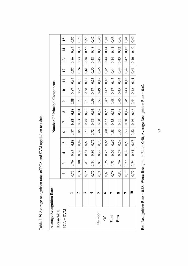
83

Tab

le 4

.29

Ave

rage

rec

ogni

tion

rat

es o

f P

CA

and

SV

M a

ppli

ed o

n te

st d

ata

Num

ber

Of

Pri

ncip

al C

ompo

nent

s A

vera

ge R

ecog

niti

on R

ates

Hie

rarc

hica

l

PC

A +

SV

M

2 3

4 5

6 7

8 9

10

11

12

13

14

15

1 0,

72

0,76

0,

85

0,88

0,

87

0,88

0,88

0,88

0,

87

0,87

0,

87

0,86

0,

85

0,85

2 0,

74

0,80

0,

86

0,87

0,

85

0,83

0,

81

0,77

0,

77

0,76

0,

74

0,73

0,

71

0,70

3 0,

75

0,81

0,

83

0,80

0,

77

0,75

0,

72

0,71

0,

68

0,64

0,

61

0,58

0,

56

0,53

4 0,

77

0,84

0,

80

0,75

0,

72

0,68

0,

63

0,59

0,

57

0,53

0,

50

0,48

0,

48

0,47

5 0,

74

0,81

0,

75

0,70

0,

66

0,60

0,

57

0,52

0,

49

0,47

0,

46

0,45

0,

45

0,45

6 0,

69

0,75

0,

72

0,65

0,

60

0,57

0,

55

0,49

0,

47

0,46

0,

45

0,44

0,

44

0,44

7 0,

78

0,73

0,

70

0,62

0,

58

0,55

0,

51

0,48

0,

47

0,45

0,

44

0,44

0,

44

0,43

8 0,

80

0,76

0,

67

0,59

0,

55

0,51

0,

48

0,46

0,

45

0,44

0,

44

0,43

0,

42

0,42

9 0,

78

0,77

0,

66

0,58

0,

53

0,50

0,

47

0,45

0,

43

0,43

0,

42

0,42

0,

42

0,41

Num

ber

Of

Tim

e

Bin

s

10

0,77

0,

74

0,64

0,

55

0,52

0,

49

0,46

0,

44

0,42

0,

41

0,41

0,

40

0,40

0,

40

Bes

t R

ecog

niti

on R

ate

= 0

.88,

Wor

st R

ecog

niti

on R

ate=

0.4

0, A

vera

ge R

ecog

niti

on R

ate

= 0

.62

84

Tab

le 4

.30

Kha

t va

lues

of

LD

A a

nd K

NN

app

lied

on

test

dat

a

N

umbe

r O

f P

rinc

ipal

Com

pone

nts

Kha

t R

esul

ts

Hie

rarc

hica

l

LD

A +

KN

N

2 3

4 5

6 7

8 9

10

11

12

13

14

15

1 0,

69

0,73

0,

70

0,70

0,

70

0,73

0,

74

0,75

0,

76

0,76

0,

74

0,76

0,

79

0,79

2 0,

78

0,79

0,

79

0,80

0,

80

0,82

0,

81

0,81

0,

80

0,80

0,

80

0,83

0,

81

0,82

3 0,

81

0,83

0,

83

0,82

0,

81

0,82

0,

81

0,82

0,

84

0,83

0,

84

0,84

0,

85

0,85

4 0,

86

0,88

0,

89

0,88

0,

89

0,88

0,

89

0,89

0,

89

0,89

0,

90

0,91

0,

90

0,89

5 0,

91

0,93

0,

92

0,92

0,

92

0,92

0,

92

0,92

0,

92

0,91

0,

91

0,92

0,

92

0,92

6 0,

94

0,94

0,

95

0,95

0,

95

0,95

0,

95

0,95

0,

94

0,94

0,

94

0,94

0,

94

0,94

7 0,

93

0,94

0,

94

0,94

0,

94

0,93

0,

94

0,94

0,

95

0,95

0,

95

0,95

0,

94

0,94

8 0,

93

0,95

0,

96

0,97

0,

96

0,97

0,

97

0,97

0,

97

0,97

0,

97

0,97

0,

96

0,97

9 0,

95

0,96

0,

97

0,97

0,98

0,

97

0,97

0,

97

0,97

0,98

0,98

0,98

0,98

0,98

Num

ber

Of

Tim

e

Bin

s

10

0,96

0,

96

0,96

0,

96

0,96

0,

96

0,95

0,

95

0,95

0,

95

0,96

0,

96

0,95

0,

96

Bes

t K

hat

Val

ue =

0.9

8, W

orst

Kha

t V

alue

= 0

.69,

Ave

rage

Kha

t V

alue

= 0

.90

85

Tab

le 4

.31

Ave

rage

rec

ogni

tion

rat

es o

f L

DA

and

KN

N a

ppli

ed o

n te

st d

ata

Num

ber

Of

Pri

ncip

al C

ompo

nent

s A

vera

ge R

ecog

niti

on R

ates

Hie

rarc

hica

l

LD

A +

KN

N

2 3

4 5

6 7

8 9

10

11

12

13

14

15

1 0,

75

0,78

0,

76

0,76

0,

76

0,78

0,

79

0,79

0,

80

0,81

0,

79

0,80

0,

83

0,83

2 0,

82

0,83

0,

83

0,83

0,

83

0,85

0,

84

0,85

0,

84

0,84

0,

83

0,86

0,

85

0,85

3 0,

85

0,86

0,

86

0,86

0,

85

0,85

0,

85

0,85

0,

87

0,86

0,

87

0,87

0,

88

0,88

4 0,

89

0,90

0,

91

0,90

0,

91

0,90

0,

91

0,91

0,

91

0,91

0,

92

0,92

0,

92

0,91

5 0,

93

0,94

0,

94

0,94

0,

94

0,93

0,

94

0,93

0,

93

0,93

0,

93

0,94

0,

94

0,94

6 0,

96

0,96

0,

96

0,96

0,

96

0,96

0,

96

0,96

0,

95

0,96

0,

95

0,95

0,

95

0,95

7 0,

95

0,95

0,

95

0,95

0,

95

0,95

0,

95

0,95

0,

96

0,96

0,

96

0,96

0,

95

0,95

8 0,

94

0,96

0,

97

0,97

0,

97

0,97

0,

97

0,98

0,98

0,98

0,

97

0,97

0,

97

0,97

9 0,

96

0,97

0,98

0,98

0,98

0,98

0,98

0,98

0,98

0,98

0,98

0,98

0,98

0,98

Num

ber

Of

Tim

e

Bin

s

10

0,97

0,

97

0,97

0,

97

0,97

0,

97

0,96

0,

96

0,96

0,

96

0,97

0,

97

0,96

0,

97

Bes

t R

ecog

niti

on R

ate

= 0

.98,

Wor

st R

ecog

niti

on R

ate=

0.7

5, A

vera

ge R

ecog

niti

on R

ate

= 0

.92

86

Tab

le 4

.32

Kha

t va

lues

of

LD

A a

nd S

VM

app

lied

on

test

dat

a

N

umbe

r O

f P

rinc

ipal

Com

pone

nts

Kha

t R

esul

ts

Hie

rarc

hica

l

LD

A +

SV

M

2 3

4 5

6 7

8 9

10

11

12

13

14

15

1 0,

67

0,72

0,

71

0,64

0,

64

0,66

0,

69

0,70

0,

72

0,71

0,

72

0,73

0,

73

0,73

2 0,

72

0,77

0,

77

0,78

0,

77

0,79

0,

77

0,81

0,

80

0,81

0,

82

0,83

0,

83

0,81

3 0,

75

0,80

0,

81

0,81

0,

81

0,80

0,

80

0,79

0,

81

0,81

0,

82

0,81

0,

81

0,82

4 0,

87

0,90

0,

88

0,88

0,

89

0,88

0,

87

0,87

0,

85

0,85

0,

84

0,85

0,

85

0,85

5 0,

92

0,93

0,

93

0,93

0,

91

0,91

0,

92

0,91

0,

91

0,92

0,

91

0,90

0,

90

0,89

6 0,

92

0,93

0,

93

0,93

0,

94

0,93

0,

94

0,94

0,

92

0,91

0,

91

0,92

0,

92

0,92

7 0,

94

0,94

0,

94

0,94

0,

94

0,93

0,

93

0,94

0,

93

0,92

0,

91

0,90

0,

91

0,90

8 0,

93

0,95

0,

94

0,95

0,

94

0,94

0,

93

0,93

0,

93

0,93

0,

93

0,93

0,

93

0,93

9 0,

93

0,96

0,97

0,97

0,

96

0,95

0,

93

0,94

0,

94

0,94

0,

94

0,94

0,

94

0,93

Num

ber

Of

Tim

e

Bin

s

10

0,94

0,

96

0,95

0,

95

0,94

0,

94

0,94

0,

94

0,93

0,

93

0,93

0,

93

0,93

0,

93

Bes

t K

hat

Val

ue =

0.9

7, W

orst

Kha

t V

alue

= 0

.64,

Ave

rage

Kha

t V

alue

= 0

.87

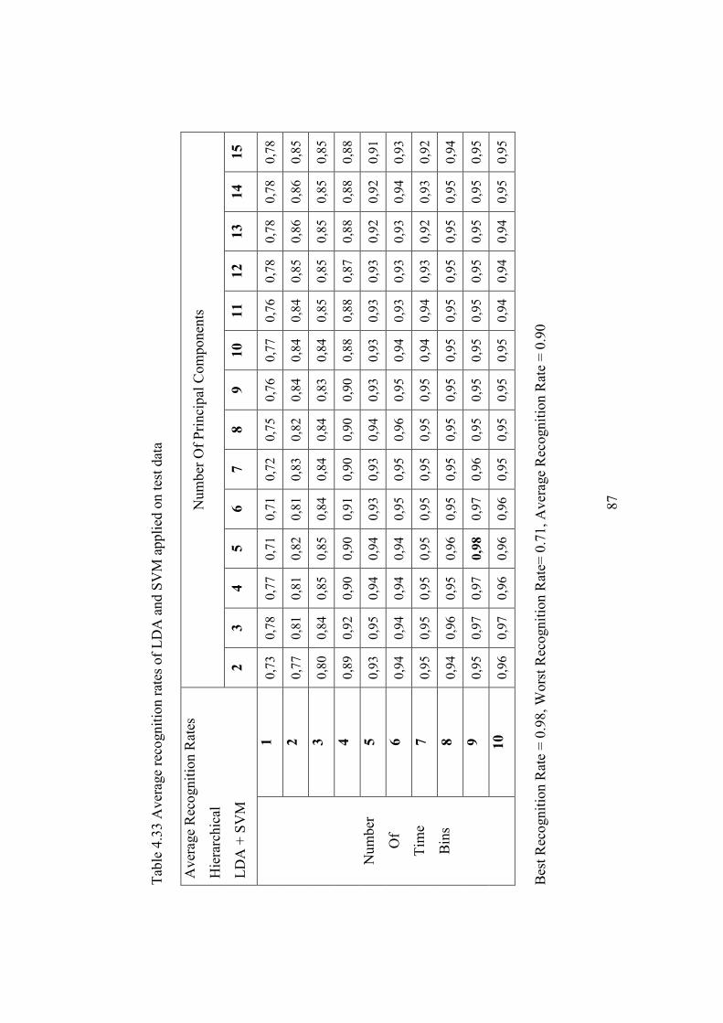
87

Tab

le 4

.33

Ave

rage

rec

ogni

tion

rat

es o

f L

DA

and

SV

M a

ppli

ed o

n te

st d

ata

Num

ber

Of

Pri

ncip

al C

ompo

nent

s A

vera

ge R

ecog

niti

on R

ates

Hie

rarc

hica

l

LD

A +

SV

M

2 3

4 5

6 7

8 9

10

11

12

13

14

15

1 0,

73

0,78

0,

77

0,71

0,

71

0,72

0,

75

0,76

0,

77

0,76

0,

78

0,78

0,

78

0,78

2 0,

77

0,81

0,

81

0,82

0,

81

0,83

0,

82

0,84

0,

84

0,84

0,

85

0,86

0,

86

0,85

3 0,

80

0,84

0,

85

0,85

0,

84

0,84

0,

84

0,83

0,

84

0,85

0,

85

0,85

0,

85

0,85

4 0,

89

0,92

0,

90

0,90

0,

91

0,90

0,

90

0,90

0,

88

0,88

0,

87

0,88

0,

88

0,88

5 0,

93

0,95

0,

94

0,94

0,

93

0,93

0,

94

0,93

0,

93

0,93

0,

93

0,92

0,

92

0,91

6 0,

94

0,94

0,

94

0,94

0,

95

0,95

0,

96

0,95

0,

94

0,93

0,

93

0,93

0,

94

0,93

7 0,

95

0,95

0,

95

0,95

0,

95

0,95

0,

95

0,95

0,

94

0,94

0,

93

0,92

0,

93

0,92

8 0,

94

0,96

0,

95

0,96

0,

95

0,95

0,

95

0,95

0,

95

0,95

0,

95

0,95

0,

95

0,94

9 0,

95

0,97

0,

97

0,98

0,

97

0,96

0,

95

0,95

0,

95

0,95

0,

95

0,95

0,

95

0,95

Num

ber

Of

Tim

e

Bin

s

10

0,96

0,

97

0,96

0,

96

0,96

0,

95

0,95

0,

95

0,95

0,

94

0,94

0,

94

0,95

0,

95

Bes

t R

ecog

niti

on R

ate

= 0

.98,

Wor

st R

ecog

niti

on R

ate=

0.7

1, A

vera

ge R

ecog

niti

on R

ate

= 0

.90

88

Tab

le 4

.34

Kha

t va

lues

of

ICA

and

KN

N a

ppli

ed o

n te

st d

ata

Num

ber

Of

Pri

ncip

al C

ompo

nent

s K

hat

Res

ults

Hie

rarc

hica

l

ICA

+ K

NN

2

3 4

5 6

7 8

9 10

11

12

13

14

15

1 0,

74

0,77

0,

80

0,80

0,

80

0,80

0,

80

0,81

0,

81

0,80

0,

81

0,81

0,

81

0,81

2 0,

75

0,82

0,

83

0,84

0,

85

0,85

0,

86

0,85

0,

84

0,84

0,

84

0,84

0,

84

0,84

3 0,

77

0,81

0,

81

0,83

0,

85

0,84

0,

85

0,85

0,

85

0,86

0,

86

0,85

0,

85

0,85

4 0,

78

0,82

0,

81

0,82

0,

83

0,83

0,

82

0,83

0,

83

0,83

0,

84

0,84

0,

84

0,85

5 0,

80

0,83

0,

84

0,85

0,

86

0,86

0,

85

0,86

0,

85

0,85

0,

85

0,85

0,

85

0,86

6 0,

82

0,83

0,

83

0,84

0,

85

0,85

0,

85

0,86

0,

86

0,85

0,

85

0,85

0,

86

0,86

7 0,

82

0,85

0,

85

0,86

0,

85

0,85

0,

86

0,86

0,87

0,

86

0,86

0,

86

0,87

0,

86

8 0,

84

0,85

0,

82

0,84

0,

83

0,83

0,

83

0,84

0,

83

0,85

0,

85

0,85

0,

85

0,86

9 0,

84

0,85

0,

86

0,86

0,

85

0,84

0,

85

0,85

0,87

0,87

0,87

0,87

0,87

0,87

Num

ber

Of

Tim

e

Bin

s

10

0,84

0,

86

0,84

0,

84

0,84

0,

83

0,83

0,

83

0,85

0,

85

0,85

0,

86

0,86

0,

86

Bes

t K

hat

Val

ue =

0.8

7, W

orst

Kha

t V

alue

= 0

.74,

Ave

rage

Kha

t V

alue

= 0

.84

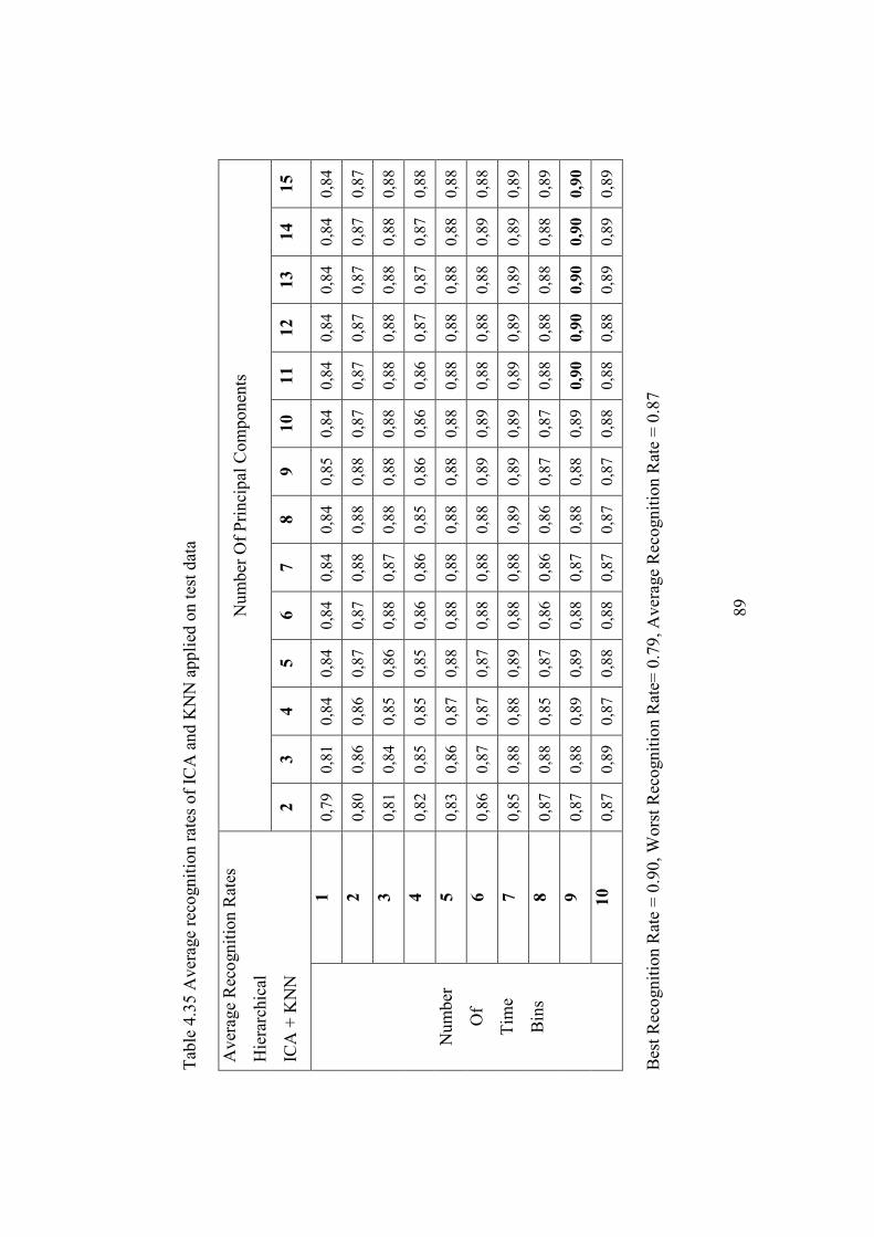
89

Tab

le 4

.35

Ave

rage

rec

ogni

tion

rat

es o

f IC

A a

nd K

NN

app

lied

on

test

dat

a

Num

ber

Of

Pri

ncip

al C

ompo

nent

s A

vera

ge R

ecog

niti

on R

ates

Hie

rarc

hica

l

ICA

+ K

NN

2

3 4

5 6

7 8

9 10

11

12

13

14

15

1 0,

79

0,81

0,

84

0,84

0,

84

0,84

0,

84

0,85

0,

84

0,84

0,

84

0,84

0,

84

0,84

2 0,

80

0,86

0,

86

0,87

0,

87

0,88

0,

88

0,88

0,

87

0,87

0,

87

0,87

0,

87

0,87

3 0,

81

0,84

0,

85

0,86

0,

88

0,87

0,

88

0,88

0,

88

0,88

0,

88

0,88

0,

88

0,88

4 0,

82

0,85

0,

85

0,85

0,

86

0,86

0,

85

0,86

0,

86

0,86

0,

87

0,87

0,

87

0,88

5 0,

83

0,86

0,

87

0,88

0,

88

0,88

0,

88

0,88

0,

88

0,88

0,

88

0,88

0,

88

0,88

6 0,

86

0,87

0,

87

0,87

0,

88

0,88

0,

88

0,89

0,

89

0,88

0,

88

0,88

0,

89

0,88

7 0,

85

0,88

0,

88

0,89

0,

88

0,88

0,

89

0,89

0,

89

0,89

0,

89

0,89

0,

89

0,89

8 0,

87

0,88

0,

85

0,87

0,

86

0,86

0,

86

0,87

0,

87

0,88

0,

88

0,88

0,

88

0,89

9 0,

87

0,88

0,

89

0,89

0,

88

0,87

0,

88

0,88

0,

89

0,90

0,90

0,90

0,90

0,90

Num

ber

Of

Tim

e

Bin

s

10

0,87

0,

89

0,87

0,

88

0,88

0,

87

0,87

0,

87

0,88

0,

88

0,88

0,

89

0,89

0,

89

Bes

t R

ecog

niti

on R

ate

= 0

.90,

Wor

st R

ecog

niti

on R

ate=

0.7

9, A

vera

ge R

ecog

niti

on R

ate

= 0

.87

90

Tab

le 4

.36

Kha

t va

lues

of

ICA

and

SV

M a

ppli

ed o

n te

st d

ata

Num

ber

Of

Pri

ncip

al C

ompo

nent

s K

hat

Res

ults

Hie

rarc

hica

l

ICA

+ S

VM

2

3 4

5 6

7 8

9 10

11

12

13

14

15

1 0,

73

0,74

0,

82

0,85

0,

87

0,85

0,

87

0,86

0,

86

0,86

0,

87

0,87

0,

86

0,87

2 0,

73

0,78

0,

82

0,81

0,

86

0,84

0,

85

0,88

0,

88

0,89

0,

90

0,90

0,

88

0,85

3 0,

78

0,83

0,

79

0,85

0,

85

0,88

0,

88

0,90

0,

88

0,88

0,

90

0,90

0,

90

0,91

4 0,

78

0,82

0,

82

0,79

0,

83

0,84

0,

88

0,90

0,

90

0,90

0,

90

0,90

0,

90

0,90

5 0,

77

0,80

0,

80

0,81

0,

84

0,88

0,

91

0,90

0,

91

0,90

0,

90

0,91

0,

91

0,91

6 0,

79

0,81

0,

80

0,80

0,

88

0,90

0,

91

0,91

0,

91

0,88

0,

88

0,89

0,

89

0,89

7 0,

77

0,79

0,

81

0,85

0,

87

0,87

0,

88

0,90

0,

91

0,90

0,

90

0,90

0,

90

0,90

8 0,

81

0,85

0,

83

0,84

0,

88

0,89

0,

90

0,89

0,

90

0,91

0,

90

0,89

0,

89

0,89

9 0,

86

0,87

0,

89

0,90

0,

93

0,92

0,

91

0,91

0,

89

0,89

0,

90

0,88

0,

90

0,92

Num

ber

Of

Tim

e

Bin

s

10

0,82

0,

87

0,90

0,

92

0,93

0,94

0,

93

0,90

0,

90

0,91

0,

90

0,91

0,

91

0,92

Bes

t K

hat

Val

ue =

0.9

4, W

orst

Kha

t V

alue

= 0

.73,

Ave

rage

Kha

t V

alue

= 0

.87

91

Tab

le 4

.37

Ave

rage

rec

ogni

tion

rat

es o

f IC

A a

nd S

VM

app

lied

on

test

dat

a

Num

ber

Of

Pri

ncip

al C

ompo

nent

s A

vera

ge R

ecog

niti

on R

ates

Hie

rarc

hica

l

ICA

+ S

VM

2

3 4

5 6

7 8

9 10

11

12

13

14

15

1 0,

78

0,79

0,

85

0,88

0,

89

0,88

0,

89

0,89

0,

89

0,89

0,

89

0,89

0,

89

0,89

2 0,

78

0,82

0,

85

0,84

0,

89

0,87

0,

87

0,90

0,

90

0,91

0,

92

0,92

0,

90

0,88

3 0,

82

0,86

0,

83

0,88

0,

87

0,90

0,

91

0,92

0,

90

0,91

0,

92

0,92

0,

92

0,93

4 0,

82

0,85

0,

86

0,83

0,

86

0,87

0,

90

0,92

0,

92

0,92

0,

92

0,92

0,

92

0,92

5 0,

82

0,84

0,

83

0,85

0,

87

0,90

0,

93

0,92

0,

93

0,92

0,

92

0,93

0,

92

0,93

6 0,

83

0,85

0,

84

0,84

0,

90

0,92

0,

93

0,93

0,

93

0,90

0,

90

0,91

0,

91

0,91

7 0,

82

0,83

0,

84

0,88

0,

89

0,89

0,

90

0,92

0,

93

0,92

0,

92

0,92

0,

92

0,92

8 0,

84

0,88

0,

87

0,87

0,

90

0,92

0,

92

0,91

0,

92

0,92

0,

92

0,91

0,

91

0,91

9 0,

88

0,89

0,

91

0,92

0,

94

0,93

0,

93

0,93

0,

92

0,91

0,

92

0,90

0,

92

0,94

Num

ber

Of

Tim

e

Bin

s

10

0,85

0,

90

0,92

0,

93

0,94

0,95

0,95

0,

92

0,92

0,

93

0,92

0,

93

0,93

0,

94

Bes

t R

ecog

niti

on R

ate

= 0

.95,

Wor

st R

ecog

niti

on R

ate=

0.7

8, A

vera

ge R

ecog

niti

on R

ate

= 0

.89

92

Tab

le 4

.38

Kha

t va

lues

of

NM

F a

nd K

NN

app

lied

on

test

dat

a

Num

ber

Of

Pri

ncip

al C

ompo

nent

s K

hat

Res

ults

Hie

rarc

hica

l

NM

F +

KN

N

2 3

4 5

6 7

8 9

10

11

12

13

14

15

1 0,

36

0,36

0,

50

0,53

0,

62

0,68

0,

72

0,71

0,

76

0,80

0,

72

0,79

0,

80

0,81

2 0,

25

0,31

0,

50

0,58

0,

68

0,66

0,

70

0,77

0,

80

0,81

0,

84

0,82

0,

86

0,88

3 0,

49

0,47

0,

55

0,61

0,

73

0,73

0,

76

0,81

0,

83

0,77

0,

86

0,86

0,

87

0,90

4 0,

30

0,54

0,

64

0,70

0,

65

0,67

0,

77

0,78

0,

78

0,80

0,

87

0,85

0,

88

0,89

5 0,

30

0,45

0,

57

0,61

0,

65

0,76

0,

80

0,84

0,

79

0,84

0,

87

0,87

0,

90

0,91

6 0,

27

0,47

0,

59

0,68

0,

77

0,73

0,

76

0,85

0,

82

0,81

0,

87

0,86

0,

89

0,90

7 0,

36

0,43

0,

58

0,63

0,

70

0,77

0,

80

0,78

0,

85

0,82

0,

87

0,89

0,

89

0,90

8 0,

36

0,49

0,

54

0,58

0,

70

0,74

0,

76

0,83

0,

84

0,88

0,

91

0,89

0,

90

0,92

9 0,

38

0,50

0,

60

0,75

0,

65

0,73

0,

82

0,83

0,

86

0,89

0,

88

0,88

0,

91

0,92

Num

ber

Of

Tim

e

Bin

s

10

0,42

0,

42

0,76

0,

68

0,75

0,

75

0,81

0,

80

0,82

0,

88

0,87

0,

89

0,92

0,94

Bes

t K

hat

Val

ue =

0.9

4, W

orst

Kha

t V

alue

= 0

.25,

Ave

rage

Kha

t V

alue

= 0

.72

93

Tab

le 4

.39

Ave

rage

rec

ogni

tion

rat

es o

f N

MF

and

KN

N a

ppli

ed o

n te

st d

ata

Num

ber

Of

Pri

ncip

al C

ompo

nent

s A

vera

ge R

ecog

niti

on R

ates

Hie

rarc

hica

l

NM

F +

KN

N

2 3

4 5

6 7

8 9

10

11

12

13

14

15

1 0,

48

0,48

0,

60

0,62

0,

69

0,74

0,

77

0,77

0,

81

0,84

0,

78

0,83

0,

84

0,85

2 0,

39

0,44

0,

60

0,66

0,

74

0,72

0,

75

0,81

0,

84

0,85

0,

87

0,86

0,

89

0,90

3 0,

59

0,57

0,

64

0,68

0,

78

0,78

0,

80

0,85

0,

87

0,82

0,

89

0,89

0,

90

0,92

4 0,

43

0,63

0,

71

0,76

0,

72

0,73

0,

81

0,83

0,

82

0,84

0,

89

0,88

0,

90

0,91

5 0,

44

0,56

0,

65

0,68

0,

71

0,81

0,

84

0,87

0,

83

0,87

0,

90

0,90

0,

92

0,93

6 0,

41

0,57

0,

67

0,75

0,

82

0,79

0,

81

0,88

0,

86

0,85

0,

89

0,88

0,

91

0,92

7 0,

49

0,54

0,

66

0,70

0,

76

0,82

0,

84

0,83

0,

88

0,85

0,

89

0,91

0,

91

0,92

8 0,

49

0,60

0,

63

0,66

0,

76

0,79

0,

81

0,87

0,

88

0,91

0,

93

0,91

0,

92

0,94

9 0,

51

0,60

0,

68

0,80

0,

72

0,78

0,

86

0,86

0,

88

0,91

0,

91

0,90

0,

93

0,93

Num

ber

Of

Tim

e

Bin

s

10

0,54

0,

53

0,81

0,

74

0,80

0,

80

0,85

0,

84

0,85

0,

91

0,90

0,

91

0,94

0,95

Bes

t R

ecog

niti

on R

ate

= 0

.95,

Wor

st R

ecog

niti

on R

ate=

0.3

9, A

vera

ge R

ecog

niti

on R

ate

= 0

.78

94

Tab

le 4

.40

Kha

t va

lues

of

NM

F a

nd S

VM

app

lied

on

test

dat

a

Num

ber

Of

Pri

ncip

al C

ompo

nent

s K

hat

Res

ults

Hie

rarc

hica

l

NM

F +

SV

M

2 3

4 5

6 7

8 9

10

11

12

13

14

15

1 0,

31

0,49

0,

52

0,57

0,

62

0,65

0,

67

0,68

0,

74

0,74

0,

74

0,76

0,

76

0,77

2 0,

33

0,43

0,

51

0,58

0,

65

0,65

0,

73

0,78

0,

79

0,81

0,

84

0,88

0,

90

0,90

3 0,

45

0,45

0,

48

0,56

0,

63

0,67

0,

72

0,78

0,

82

0,83

0,

85

0,89

0,

90

0,91

4 0,

38

0,44

0,

50

0,63

0,

66

0,68

0,

78

0,80

0,

82

0,84

0,

89

0,88

0,

92

0,92

5 0,

33

0,47

0,

52

0,57

0,

61

0,72

0,

77

0,79

0,

82

0,84

0,

87

0,90

0,

90

0,90

6 0,

36

0,48

0,

54

0,63

0,

71

0,67

0,

72

0,82

0,

84

0,87

0,

88

0,89

0,

91

0,92

7 0,

33

0,40

0,

56

0,56

0,

69

0,73

0,

78

0,81

0,

86

0,87

0,

89

0,91

0,

90

0,91

8 0,

40

0,42

0,

48

0,54

0,

63

0,72

0,

78

0,81

0,

84

0,88

0,

91

0,93

0,

92

0,92

9 0,

38

0,46

0,

52

0,55

0,

61

0,75

0,

82

0,82

0,

86

0,89

0,

91

0,92

0,

92

0,92

Num

ber

Of

Tim

e

Bin

s

10

0,34

0,

41

0,51

0,

58

0,69

0,

73

0,80

0,

80

0,83

0,

89

0,88

0,

90

0,92

0,

91

Bes

t K

hat

Val

ue =

0.9

3, W

orst

Kha

t V

alue

= 0

.31,

Ave

rage

Kha

t V

alue

= 0

.71

95

Tab

le 4

.41

Ave

rage

rec

ogni

tion

rat

es o

f N

MF

and

SV

M a

ppli

ed o

n te

st d

ata

Num

ber

Of

Pri

ncip

al C

ompo

nent

s A

vera

ge R

ecog

niti

on R

ates

Hie

rarc

hica

l

NM

F +

SV

M

2 3

4 5

6 7

8 9

10

11

12

13

14

15

1 0,

45

0,59

0,

62

0,65

0,

69

0,72

0,

73

0,74

0,

79

0,79

0,

79

0,80

0,

81

0,81

2 0,

47

0,54

0,

60

0,66

0,

72

0,71

0,

78

0,82

0,

83

0,85

0,

87

0,90

0,

92

0,92

3 0,

56

0,56

0,

58

0,64

0,

70

0,74

0,

78

0,82

0,

85

0,86

0,

88

0,91

0,

92

0,93

4 0,

50

0,55

0,

60

0,70

0,

73

0,75

0,

82

0,84

0,

85

0,87

0,

91

0,90

0,

93

0,94

5 0,

46

0,57

0,

61

0,65

0,

69

0,77

0,

81

0,83

0,

85

0,87

0,

90

0,92

0,

92

0,92

6 0,

49

0,58

0,

63

0,70

0,

77

0,74

0,

77

0,86

0,

87

0,90

0,

90

0,92

0,

93

0,93

7 0,

47

0,51

0,

64

0,65

0,

75

0,78

0,

83

0,85

0,

89

0,90

0,

91

0,92

0,

92

0,93

8 0,

52

0,54

0,

58

0,63

0,

70

0,77

0,

82

0,85

0,

88

0,91

0,

93

0,94

0,94

0,94

9 0,

50

0,57

0,

62

0,65

0,

69

0,80

0,

85

0,86

0,

89

0,91

0,

93

0,94

0,

93

0,94

Num

ber

Of

Tim

e

Bin

s

10

0,48

0,

53

0,61

0,

66

0,76

0,

79

0,84

0,

84

0,86

0,

91

0,91

0,

92

0,93

0,

93

Bes

t R

ecog

niti

on R

ate

= 0

.94,

Wor

st R

ecog

niti

on R

ate=

0.4

5, A

vera

ge R

ecog

niti

on R

ate

= 0

.77

96

Observing the classification performance tables of normal classification and

hierarchical classification, we can conclude that hierarchical classification does

not provide classification performance improvement for all feature extraction

and classification methods. Hierarchical classification improves classification

performance around %3-4 for LDA+KNN and LDA+SVM. Hierarchical

classification does not improve performance for PCA+SVM, ICA+SVM,

NMF+KNN, NMF+SVM. We can conclude that hierarchical classification does

not improve performance when SVM or NMF is used. Also a classification

performance improvement of %2 is obtained for PCA+KNN, ICA+KNN.

Hierarchical classification improves performance when KNN is used.

4.4 Confusion Matrices

Khat values and average recognition rates for different number of time-

bins and principal components were given through Table 4.9 to Table 4.25 for

normal classification. Observing these tables we can see that best classification

results are obtained with LDA+SVM and ICA+SVM. From Table 4.17, we see

that an average recognition rate of %98 is obtained with LDA+SVM when the

number of time bins is 9 and number of principal components is 12. The

recognition rate obtained with LDA+SVM is %76, when the number of time

bins is 1 and number of principal components is 12. To see the performance

improvement by increasing the number of time-bins, confusion matrices for

these two cases are given in Table 4.42 and Table 4.43 .

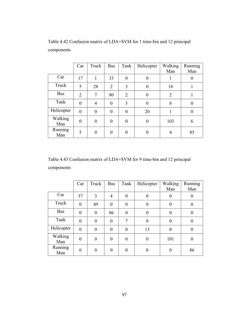
97


components

Car Truck Bus Tank Helicopter Walking

Man Running

Man Car 17 1 33 0 0 1 0

Truck 5 28 2 3 0 18 1

Bus 2 7 80 2 0 2 1

Tank 0 4 0 3 0 8 0

Helicopter 0 0 0 0 20 1 0

Walking Man

0 0 0 0 0 103 6

Running Man

5 0 0 0 0 4 85


components


Man Running

Man Car 37 3 4 0 0 0 0

Truck 0 49 0 0 0 0 0

Bus 0 0 86 0 0 0 0

Tank 0 0 0 7 0 0 0


Walking Man

0 0 0 0 0 101 0

Running Man

0 0 0 0 0 0 86

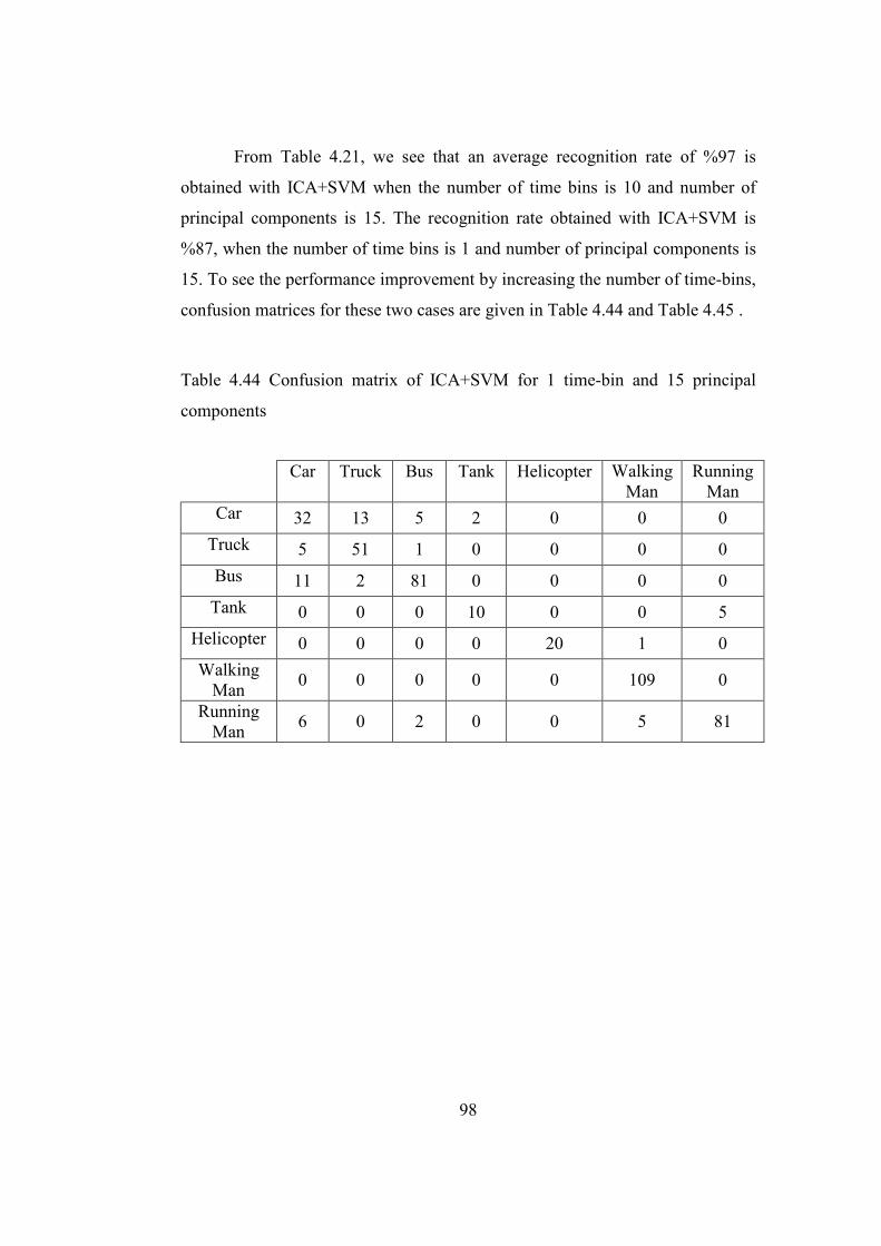
98

From Table 4.21, we see that an average recognition rate of %97 is

obtained with ICA+SVM when the number of time bins is 10 and number of

principal components is 15. The recognition rate obtained with ICA+SVM is

%87, when the number of time bins is 1 and number of principal components is

15. To see the performance improvement by increasing the number of time-bins,

confusion matrices for these two cases are given in Table 4.44 and Table 4.45 .

Table 4.44 Confusion matrix of ICA+SVM for 1 time-bin and 15 principal

components


Man Running

Man Car 32 13 5 2 0 0 0

Truck 5 51 1 0 0 0 0

Bus 11 2 81 0 0 0 0

Tank 0 0 0 10 0 0 5


Walking Man

0 0 0 0 0 109 0

Running Man

6 0 2 0 0 5 81

99

Table 4.45 Confusion matrix of ICA+SVM for 10 time-bins and 15 principal

components


Man Running

Man Car 37 0 6 0 0 0 0

Truck 0 47 1 0 0 0 0

Bus 0 0 83 2 0 0 0

Tank 0 0 0 6 0 0 0


Walking Man

0 0 0 0 0 100 0

Running Man

3 0 1 0 0 0 81

4.5 Classification Performance Summary

The summary of the classification performance results is given in Table 4.42.

This summary table contains the best, worst and average classification

performances of the tables Table 4.9 through Table 4.41.

10

0

Tab

le 4

.46

Sum

mar

y of

cla

ssif

icat

ion

perf

orm

ance

tab

les

Normal Classification

Hierarchical Classification

KHAT

VALUE

RECOGNITIO

N

RATE

KHAT

VALUE

RECOGNITIO

N

RATE

CLASSIFIC

ATIO

N

FEATURE

EXTRACTIO

N

Best

Worst

Average

Best

Worst

Average

Best

Worst

Average

Best

Worst

Average

PC

A

0.92

0.

69

0.89

0.

94

0.75

0.

91

0.94

0.

76

0.90

0.

95

0.80

0.

92

LD

A

0.94

0.

53

0.86

0.

95

0.61

0.

88

0.98

0.

69

0.90

0.

98

0.75

0.

92

ICA

0.

84

0.73

0.

81

0.87

0.

78

0.85

0.

87

0.74

0.

84

0.90

0.

79

0.87

KNN

NM

F

0.89

0.

21

0.72

0.

91

0.36

0.

77

0.94

0.

25

0.72

0.

95

0.39

0.

78

PC

A

0.87

0.

29

0.65

0.

90

0.47

0.

73

0.86

0.

19

0.50

0.

88

0.40

0.

62

LD

A

0.98

0.

52

0.84

0.

98

0.61

0.

87

0.97

0.

64

0.87

0.

98

0.71

0.

90

ICA

0.

97

0.79

0.

87

0.97

0.

83

0.89

0.

94

0.73

0.

87

0.95

0.

78

0.89

SVM

NM

F

0.97

0.

33

0.74

0.

97

0.47

0.

79

0.93

0.

31

0.71

0.

94

0.45

0.

77

101

CHAPTER 5

CONCLUSION

In this thesis improving the classification performance of the target recognition

system designed in Erdogan (2002) is studied. Classification performance

improvement is done by the following methods:

• Utilizing the repetitions in time in the TRP vectors of some target classes

(walking man, running man and helicopter).

• Using different feature extraction (PCA, LDA, ICA and NMF) and

classifier (KNN, SVM) combinations.

• Hierarchical Classification.

We observed that best classification performance results are obtained

with LDA+SVM and ICA+SVM. ICA+SVM provides a minimum recognition

rate of %83 and maximum recognition rate of %97. Also maximum recognition

rate of LDA+SVM is %98, however ICA+SVM outperforms LDA+SVM at

minimum recognition performance, the minimum recognition rate for

LDA+SVM is %61. For all feature extraction and classification method

combinations increasing the number of time bins also increases classification

performance except PCA+SVM. For higher number of time bins and principal

components NMF+KNN and NMF+SVM provides good classification

performance (maximum recognition rates of %90 and %96 respectively),

however NMF performance is not good for small number of time bins and

principal components. Also NMF is not real time implementable; it takes too

much time to extract features. Among the feature extraction methods ICA is the

most useful one to extract the important features of the input data with the

minimum number of principal components. A recognition rate of %83 is

102

obtained when the number of time bins is 1 and the number of principal

components is 2. Also SVM provides better performance than KNN.

Hierarchical classification does not improve classification performance

except LDA method. But this improvement becomes insignificant when the

number of principal components is high. When the number of principal

components is 2 and number of time bins is 1, LDA+SVM provides a

recognition rate of %61 for normal classification and %73 for hierarchical

classification. When the number of principal components is 2 and number of

time bins is 10, LDA+SVM provides a classification performance of %77 for

normal classification and % 96 for hierarchical classification. Hierarchical

classfication can be used to increase the performance of LDA, but there is no

need to use such a method for ICA since hierarchical classification makes our

target recognition system more complex.

Future research may consider the optimal target recognition system in

which each type of misclassification brings different costs to the system. Since

the radar used is a military radar, the classification of a car target as running

man is more dangerous than classifying a walking man target as running man.

The future work can study on a target recognition system which will minimize

such dangerous misclassifications. Also multiple target situations are not

handled in the thesis, they can be considered at a future work.

103

REFERENCES

[1] Bilik I., Tabrikian J. and Cohen A., “Target Classification Using Gaussian Mixture Model for Ground Surveillance Doppler Radar”, in IEEE International Radar Conference, 2005, pp. 910-915.

[2] Bullard B. D. and Dowdy P. C., “Pulse Doppler Signature of a Rotary

Wing Aircraft”, IEEE AES Systems Magazine, 1991. [3] Castalez P.F., “Neural Networks in Defense Applications”, in IEEE

International Conference On Neural Networks, 1988, pp. 473-480. [4] Chen V.C., “Analysis of Radar Micro-Doppler Signature with Time-

Frequency Transform”, in Proceedings of the Tenth IEEE Workshop on

Statistical Signal and Array Processing, 2000, pp. 463-466. [5] Erdogan A., ”Doppler Radar Target Recognition by Neural Networks”,

Doctorate Thesis, Metu Computer Vision and Intelligent Systems Laboratory, 2002.

[6] Hyvarinen A., “Survey On Independent Component Analysis”, Neural

Computing Surveys, pp. 94-128, 1999. [7] Jianjun H., Jingxiong H. and Weixin X., “Target Classification by

Conventional Radar”, in Proceedings of CIE International Conference

on Radar, 1996, pp. 204-207. [8] Lathauwer L., “An Introduction to Independent Component Analysis”,

Journal of Chemometrics 2000, pp. 123-149, 2000. [9] Lei J. and Lu C., “Target Classification Based on Micro-Doppler Radar

Signatures”, in IEEE International Radar Conference, 2005. [10] Madrid J.J.M., Corredera J.R.C. and Vela G.M., “A Neural Network

Approach to Doppler-Based Target Classification”, in Radar 92.

International Conference, 1992, pp. 450-453.

104

[11] McConaghy T., Leung H., Bossé E., and Varadan V, “Classification of Audio Radar Signals Using Radial Basis Function Neural Networks”, IEEE Transactions on Instrumentation and Measurement, vol. 52, issue: 6, pp. 1771- 1779, 2003.

[12] Richards M.A., Fundamentals of Radar Signal Processing, McGraw-

Hill, 2005. [13] Schweitzer H., “Utilizing Scatter for Pixel Subspace Selection”, in

Proceedings of the Seventh IEEE International Conference on Computer

Vision, 1999, pp. 1111-1116.

[14] Shan S. and Cao B., “Extended Fisherface for Face Recognition from a Single Image per Person”, in IEEE Internatonal Symposium on Circuits

ad Systems, 2002, vol. 2, pp. 81-84.

[15] Shlens J., “A Tutorial on Principal Component Analysis”, December 2005. , http://www.snl.salk.edu/~shlens/pub/notes/pca.pdf , Last accessed 26 June 2008.

[16] Skolnik M.I., Introduction to Radar Systems, McGraw-Hill, 2001.

[17] Spider Support Vector Machine Tool, July 2006, Version 1.7, http://www.kyb.tuebingen.mpg.de/bs/people/spider/, Last accessed 26 June 2008.

[18] Stimson G.W., Introduction to Airborne Radar, SciTech Publishing Inc, 1998.

[19] Stove A.G. and Sykes S.R, “A Doppler Based Automatic Target Classifier for a Battlefield Surveillance Radar”, in RADAR 2002, 2002, pp. 419-423.

[20] Üstün B., 3-D Face Recognition, Master Thesis, Metu Computer Vision and Intelligent Systems Laboratory, 2007

[21] Vasilescu M.A.O., “Multilinear Independent Component Analysis”, in IEEE Computer Society Conference on Computer Vision and Pattern

Recognition, 2005.

[22] Weixiang L. and Nanning Z., “Non-negative Matrix Factorization and Its Applications in Pattern Recognition”, Chinese Science Bulletin 2006, vol. 21, no: 17-18, 2006.

105

[23] Wilkinson G.G., “Results and Implications of a Study of Fifteen Years of Satellite Image Classification Experiments”, IEEE Transactions on

Geoscience and Remote Sensing, pp. 433-440, 2005.

[24] Xue Y. and Tong C.S., “A Modified Non-negative Matrix Factorization Algorithm for Face Recognition”, in The 18

th International Conference

on Pattern Recognition, 2006.

[25] Yoon S., Kim B. and Kim Y., “Helicopter Classification Using Time-Frequency Analysis”, Electronic Letters, pp. 1871-1872, 2000.

[26] Zardoshti M, Wheeler B.C., Badie K. and Hashemi R., “Evaluation of EMG Features for Movement Control of Prostheses”, 1993, http://www.ieeexplore.ieee.org/iel4/86/10234/00481972.pdf, Last accessed 26 June 2008.

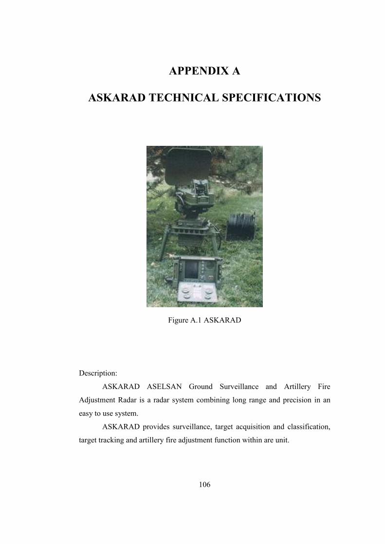
106

APPENDIX A

ASKARAD TECHNICAL SPECIFICATIONS

Figure A.1 ASKARAD

Description:

ASKARAD ASELSAN Ground Surveillance and Artillery Fire

Adjustment Radar is a radar system combining long range and precision in an

easy to use system.

ASKARAD provides surveillance, target acquisition and classification,

target tracking and artillery fire adjustment function within are unit.

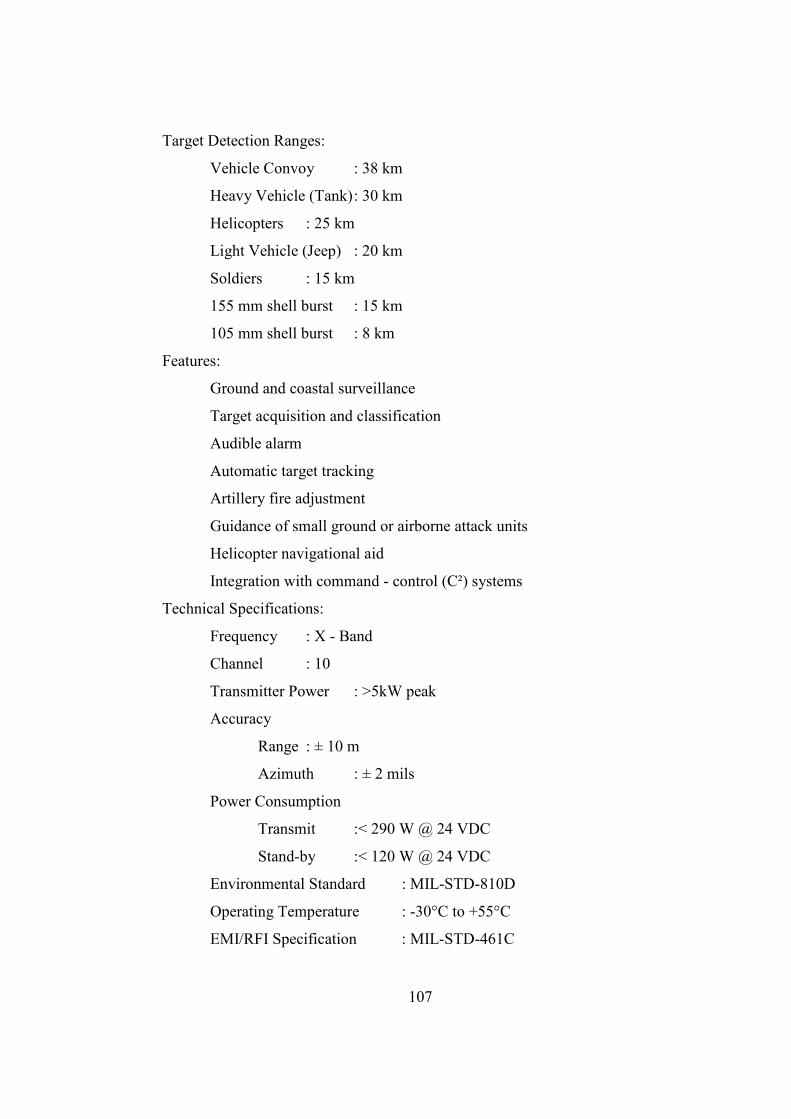
107

Target Detection Ranges:

Vehicle Convoy : 38 km

Heavy Vehicle (Tank) : 30 km

Helicopters : 25 km

Light Vehicle (Jeep) : 20 km

Soldiers : 15 km

155 mm shell burst : 15 km

105 mm shell burst : 8 km

Features:

Ground and coastal surveillance

Target acquisition and classification

Audible alarm

Automatic target tracking

Artillery fire adjustment

Guidance of small ground or airborne attack units

Helicopter navigational aid

Integration with command - control (C²) systems

Technical Specifications:

Frequency : X - Band

Channel : 10

Transmitter Power : >5kW peak

Accuracy

Range : ± 10 m

Azimuth : ± 2 mils

Power Consumption

Transmit :< 290 W @ 24 VDC

Stand-by :< 120 W @ 24 VDC

Environmental Standard : MIL-STD-810D

Operating Temperature : -30°C to +55°C

EMI/RFI Specification : MIL-STD-461C

Documents

DOPPLER RADAR DATA PROCESSING AND … · kullanılan radar doppler tabanlı bir kara gözetleme radarıdır. Hedef tipleri ise araba, kamyon, ... APPENDIX A ASKARAD TECHNICAL SPECIFICATIONS