Embed Size (px)
Citation preview

Trends and cycles in the Euro area: how
much heterogeneity and should we worry
about it?
Domenico Giannone
DGR-ECB, Universite Libre de Bruxelles
(ECARES)
Lucrezia Reichlin
DGR-ECB and CEPR
Fourth Macroeconomic Policy Research Workshopon Nominal Exchange rates and the real economy,
Budapest 29-30 September 2005
1

Old and recent debate
Before the EMU: optimal currency area debate (hetero-geneity)
After 6 years: have things changed?
This paper look at the issue from a narrow perspective
• analyze output differentials within EMU in the lastthirty years: levels, growth, recessions
• ask whether heterogeneous dynamics is generatedby national/idiosyncratic shocks or heterogeneousresponse to Euro-wide shock
• ask whether Euro-wide shocks should be interpretedas world (US) shocks
• ask whether consumption correlations conditionalon output have changed over the last years (risksharing)
2
Four Findings
1. Asymmetries in output per capita (whatever
the concept) between the Euro area countries
have remained roughly the same in the last
thirty years (+ similar to asymmetries within
the US)
2. Asymmetries mainly explained by small but
persistent idiosyncratic shocks while the bulk
of output fluctuation are explained by a com-
mon shock
3. The common shock can be interpreted as
a US shock that affects the Euro area with a
lag and generates a Euro cycle that is more
persistent but less volatile than the US’s.
4. Risk-sharing within the Euro area has in-
creased since the early 1990s.
3
STEP 1: Look at levels of output per capita
Why?
It is what goes into people’s pockets
Define
yit ×100 log of real GDP per-capita of country
i in year t (PPP adjusted).
gapit = yi
t − yEUt : percentage deviation of real
GDP per-capita of country i from Euro
Area.
Measure of asymmetry 1: gapit
4
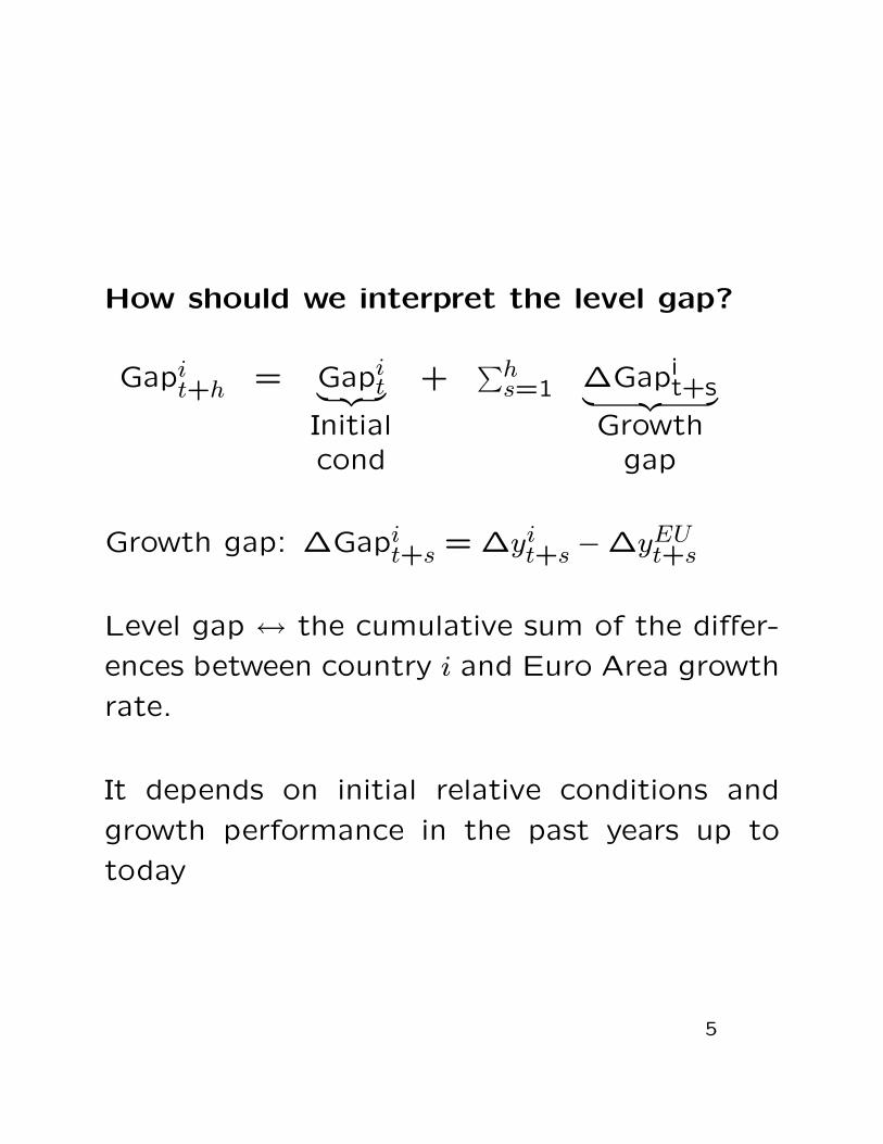
How should we interpret the level gap?
Gapit+h = Gapi
t︸ ︷︷ ︸ +∑h
s=1 ∆Gapit+s︸ ︷︷ ︸
Initial Growthcond gap
Growth gap: ∆Gapit+s = ∆yi
t+s −∆yEUt+s
Level gap ↔ the cumulative sum of the differ-
ences between country i and Euro Area growth
rate.
It depends on initial relative conditions and
growth performance in the past years up to
today
5

Questions
1. How large are the asymmetries?
2. How do they evolve over time?
3. Do the differences in growth rates (growth
gap) cancel out over time (the last 30 years)
or are they persistent?
4. Clubs or convergence?
Table + Plots
6
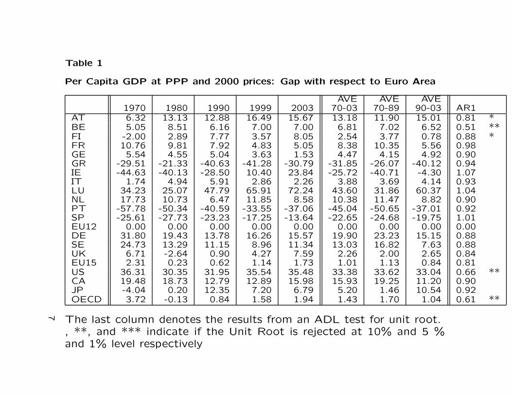
Table 1
Per Capita GDP at PPP and 2000 prices: Gap with respect to Euro Area
AVE AVE AVE1970 1980 1990 1999 2003 70-03 70-89 90-03 AR1
AT 6.32 13.13 12.88 16.49 15.67 13.18 11.90 15.01 0.81 *BE 5.05 8.51 6.16 7.00 7.00 6.81 7.02 6.52 0.51 **FI -2.00 2.89 7.77 3.57 8.05 2.54 3.77 0.78 0.88 *FR 10.76 9.81 7.92 4.83 5.05 8.38 10.35 5.56 0.98GE 5.54 4.55 5.04 3.63 1.53 4.47 4.15 4.92 0.90GR -29.51 -21.33 -40.63 -41.28 -30.79 -31.85 -26.07 -40.12 0.94IE -44.63 -40.13 -28.50 10.40 23.84 -25.72 -40.71 -4.30 1.07IT 1.74 4.94 5.91 2.86 2.26 3.88 3.69 4.14 0.93LU 34.23 25.07 47.79 65.91 72.24 43.60 31.86 60.37 1.04NL 17.73 10.73 6.47 11.85 8.58 10.38 11.47 8.82 0.90PT -57.78 -50.34 -40.59 -33.55 -37.06 -45.04 -50.65 -37.01 0.92SP -25.61 -27.73 -23.23 -17.25 -13.64 -22.65 -24.68 -19.75 1.01EU12 0.00 0.00 0.00 0.00 0.00 0.00 0.00 0.00 0.00DE 31.80 19.43 13.78 16.26 15.57 19.90 23.23 15.15 0.88SE 24.73 13.29 11.15 8.96 11.34 13.03 16.82 7.63 0.88UK 6.71 -2.64 0.90 4.27 7.59 2.26 2.00 2.65 0.84EU15 2.31 0.23 0.62 1.14 1.73 1.01 1.13 0.84 0.81US 36.31 30.35 31.95 35.54 35.48 33.38 33.62 33.04 0.66 **CA 19.48 18.73 12.79 12.89 15.98 15.93 19.25 11.20 0.90JP -4.04 0.20 12.35 7.20 6.79 5.20 1.46 10.54 0.92OECD 3.72 -0.13 0.84 1.58 1.94 1.43 1.70 1.04 0.61 **
The last column denotes the results from an ADL test for unit root., **, and *** indicate if the Unit Root is rejected at 10% and 5 %and 1% level respectively
7
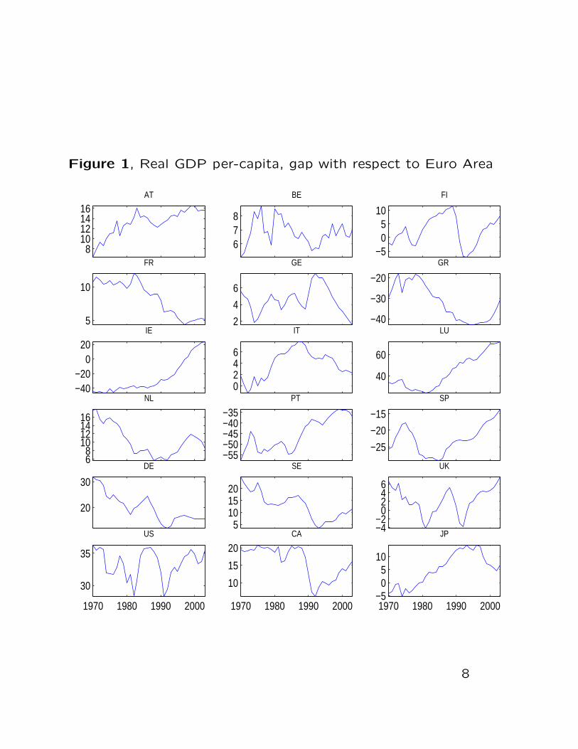
Figure 1, Real GDP per-capita, gap with respect to Euro Area
810121416
AT
678
BE
−505
10
FI
5
10
FR
2
4
6
GE
−40
−30
−20
GR
−40−20
020
IE
0246
IT
40
60
LU
68
10121416
NL
−55−50−45−40−35
PT
−25
−20
−15
SP
20
30
DE
5101520
SE
−4−2
0246
UK
1970 1980 1990 2000
30
35
US
1970 1980 1990 2000
10
15
20CA
1970 1980 1990 2000−5
05
10
JP
8
Results
1. The gap of Euro Area countries are persistent / non-stationary → no clear tendency of convergence towarda common level of income (no common trend)
Exceptions: Spain and Ireland (convergence?)
No sign of changes recently [impossible to detect givenpersistency]
2. The gap between US as a whole and EMU aggregateis less persistent / stationary → US citizen have been onaverage in the three decades 33% richer than Europeansand the gap has been fluctuating around this value
9

Is the lack of common trend between Euro
countries and Euro aggregate explained by
convergence dynamics?
The Literature:
Harvey, 2005: Rich countries stay close to
average and poor countries (Greece, Portu-
gal, Spain) converged to a low level of out-
put around 30% below average [Ireland is an
exception]
Our point:
These predictions are difficult and unreliable
since gaps are very persistent, hence their long
run behavior is difficult to predict
For example, looking at the last few years there
appears to be a tendency for the Spanish gap
to close, contrary to what predicted by Harvey
10
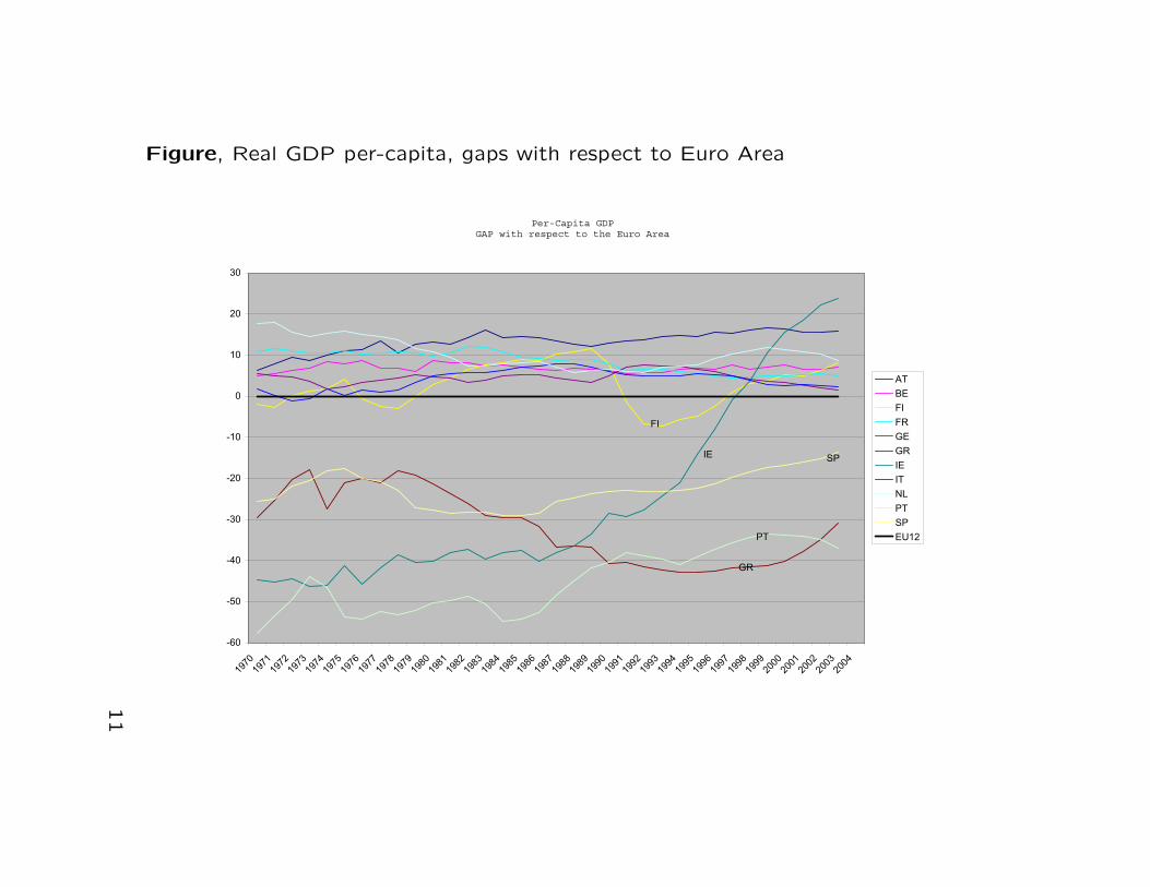
Figure, Real GDP per-capita, gaps with respect to Euro Area
Per-Capita GDPGAP with respect to the Euro Area
FI
GR
IE
PT
SP
-60
-50
-40
-30
-20
-10
0
10
20
30
1970
1971
1972
1973
1974
1975
1976
1977
1978
1979
1980
1981
1982
1983
1984
1985
1986
1987
1988
1989
1990
1991
1992
1993
1994
1995
1996
1997
1998
1999
2000
2001
2002
2003
2004
AT
BE
FI
FR
GE
GR
IE
IT
NL
PT
SP
EU12
11
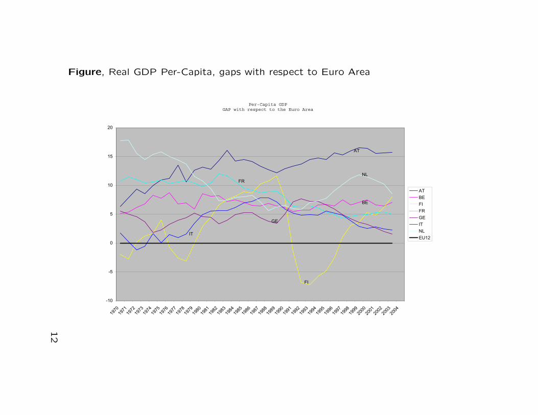
Figure, Real GDP Per-Capita, gaps with respect to Euro Area
Per-Capita GDPGAP with respect to the Euro Area
AT
BE
FI
FR
GE
IT
NL
-10
-5
0
5
10
15
20
1970
1971
1972
1973
1974
1975
1976
1977
1978
1979
1980
1981
1982
1983
1984
1985
1986
1987
1988
1989
1990
1991
1992
1993
1994
1995
1996
1997
1998
1999
2000
2001
2002
2003
2004
AT
BE
FI
FR
GE
IT
NL
EU12
12
STEP 2: Cyclical asymmetry: outptut per
capita
Measures of asymmetry 2: growth rates
How large is the growth rate gap?
Var(∆yit −∆yEU
t )
Cfr. Figure
13
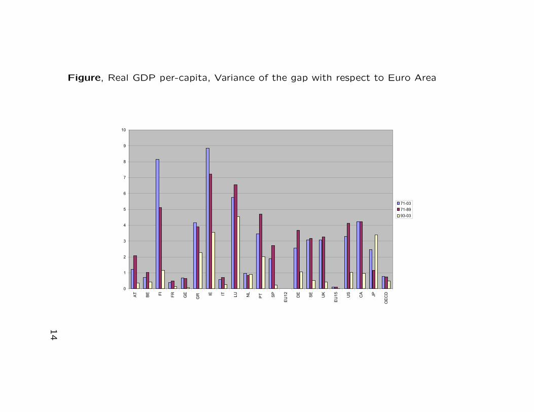
Figure, Real GDP per-capita, Variance of the gap with respect to Euro Area
0
1
2
3
4
5
6
7
8
9
10
AT
BE FI
FR
GE
GR IE IT LU
NL
PT
SP
EU
12
DE
SE
UK
EU
15
US
CA
JP
OE
CD
71-03
71-89
93-03
14
• Decrease in asymmetry? NO!!
- Need to control for size of output fluctuations
Var(∆yit)
cfr. Figure
15
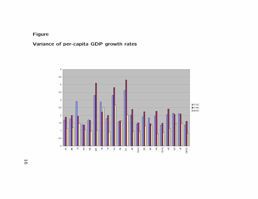
Figure
Variance of per-capita GDP growth rates
0
0.5
1
1.5
2
2.5
3
3.5
4
4.5
5
AT
BE FI
FR
GE
GR IE IT LU
NL
PT
SP
EU
12
DE
SE
UK
EU
15
US
CA
JP
OE
CD
71-03
71-89
93-03
16

• Variance has decreased everywhere
=⇒ The“great moderation” is a worldwide phe-
nomenon
eg. Stock and Watson, huge literature...
17

Controlling for the great moderation
How correlated if growth growth of country i
with the Euro area?
Corr(∆yit,∆yEU
t )
cfr. Figure
18
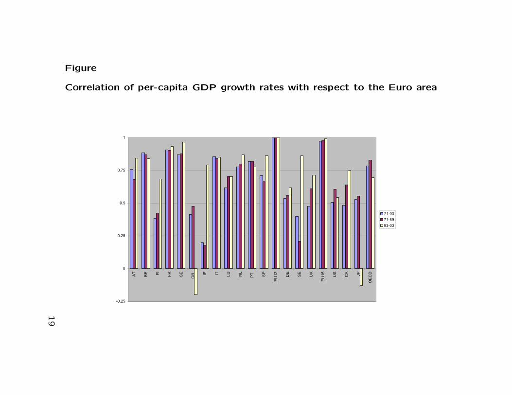
Figure
Correlation of per-capita GDP growth rates with respect to the Euro area
-0.25
0
0.25
0.5
0.75
1A
T
BE FI
FR
GE
GR IE IT LU
NL
PT SP
EU
12
DE
SE
UK
EU
15
US
CA
JP
OE
CD
71-03
71-89
93-03
19

Comments
• Cyclical comovement is high and stable within
the Euro Area and between Euro area and the
rest of the world...
⇒ Stability: Stock and Watson
⇒ Large world business cycle: Kose et al.,
Canova et al., Montfort et al., Artis and coau-
thors, Madrid Conference ...
• Comovement is higher within Euro area than
between the Euro area and the rest of the
world.
Euro area cycle? See later...
Remark
Asymmetry 1 (levels) vs Asymmetry 2 (cycle)
See later20

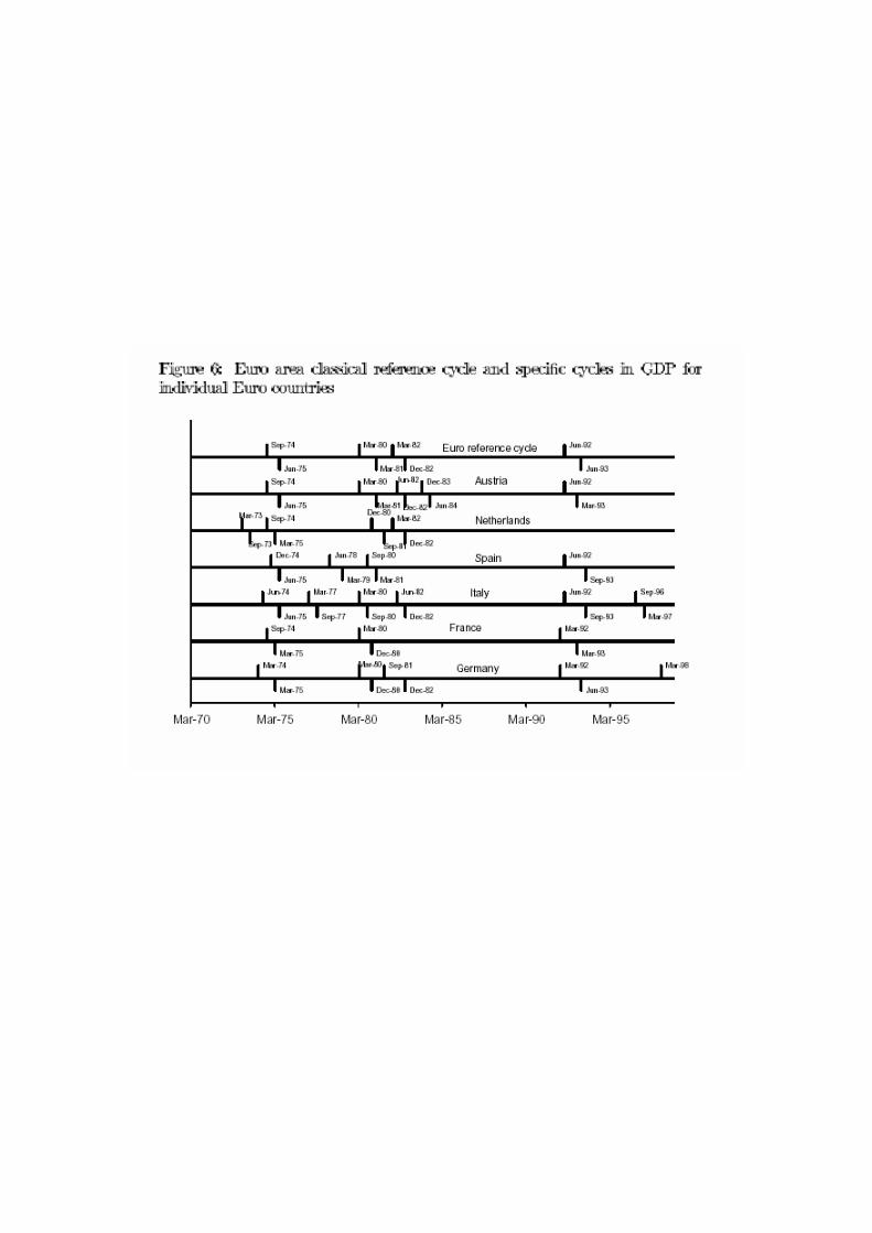
STEP 2: Cyclical asymmetry output per capita
Measure of asymmetry 3: recessions
cfr. Harding and Pagan dating
=⇒ Cycles are very synchronized, within the
Euro area
For EU and Rest of the World see later
21

Summary
• Great moderation
⇒ Worldwide phenomenon
• Cyclical asymmetry: small and stable whitin
the Euro area and between the Euro area and
the Rest of the World
• Higher comovement within the Euro area:
Euro area cycle different from world cycle?
• Asymmetries in levels are small but persis-
tent: they do not cancel out as time passes
by...
22
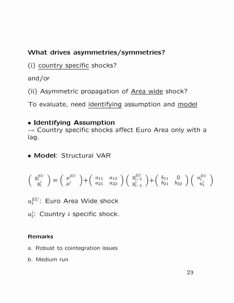
What drives asymmetries/symmetries?
(i) country specific shocks?
and/or
(ii) Asymmetric propagation of Area wide shock?
To evaluate, need identifying assumption and model
• Identifying Assumption→ Country specific shocks affect Euro Area only with alag.
• Model: Structural VAR
(yEU
tyi
t
)=(
µEU
µi
)+(
a11 a12a21 a22
)(yEU
t−1yi
t−1
)+(
b11 0b21 b22
)(uEU
tui
t
)uEU
t : Euro Area Wide shock
uit: Country i specific shock.
Remarks
a. Robust to cointegration issues
b. Medium run
23
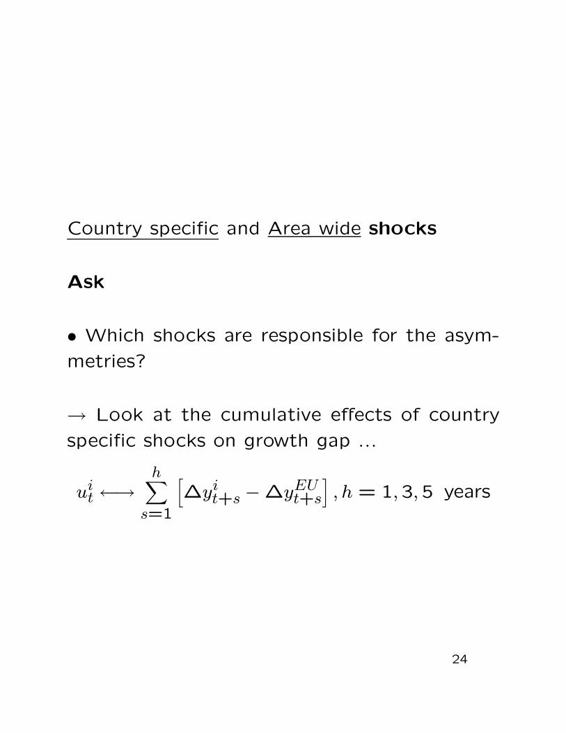
Country specific and Area wide shocks
Ask
• Which shocks are responsible for the asym-
metries?
→ Look at the cumulative effects of country
specific shocks on growth gap ...
uit←→
h∑s=1
[∆yi
t+s −∆yEUt+s
], h = 1,3,5 years
24
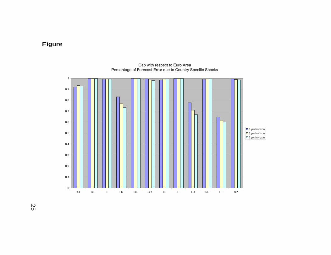
Figure
Gap with respect to Euro Area
Percentage of Forecast Error due to Country Specific Shocks
0
0.1
0.2
0.3
0.4
0.5
0.6
0.7
0.8
0.9
1
AT BE FI FR GE GR IE IT LU NL PT SP
0 yrs horizon
3 yrs horizon
5 yrs horizon
25

Country specific and Area wide shocks
Ask
• Which shocks are responsible for the asym-
metries?
Answer
Gap is mainly explained by country specific shocks
at all horizons
26
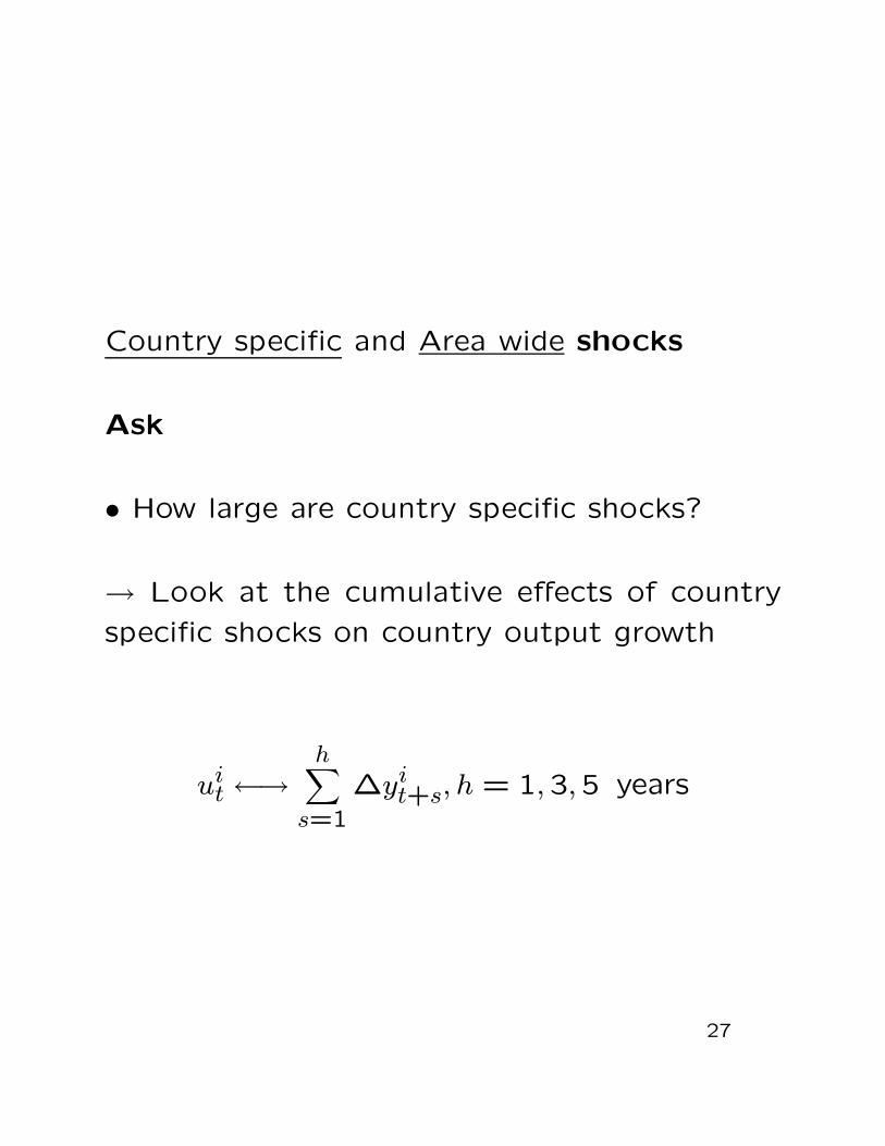
Country specific and Area wide shocks
Ask
• How large are country specific shocks?
→ Look at the cumulative effects of country
specific shocks on country output growth
uit ←→
h∑s=1
∆yit+s, h = 1,3,5 years
27
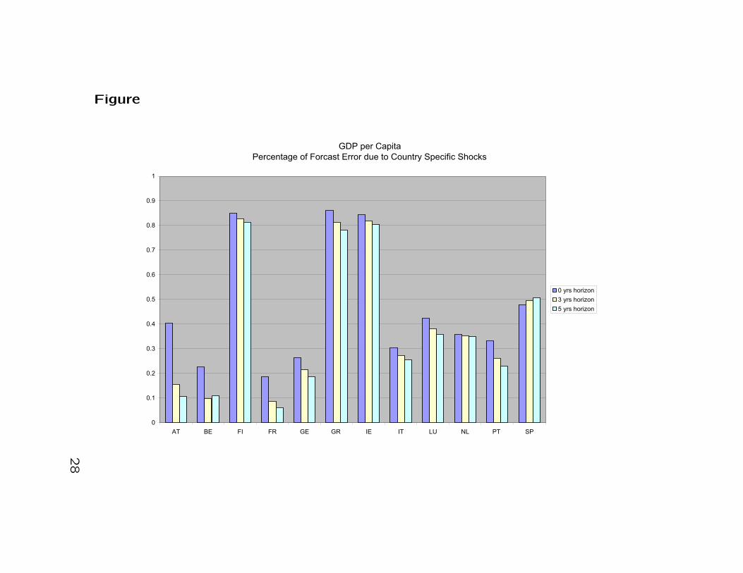
Figure
GDP per Capita
Percentage of Forcast Error due to Country Specific Shocks
0
0.1
0.2
0.3
0.4
0.5
0.6
0.7
0.8
0.9
1
AT BE FI FR GE GR IE IT LU NL PT SP
0 yrs horizon
3 yrs horizon
5 yrs horizon
28

Country specific and Area wide shocks
Ask
• How large are country specific shocks?
Answer
• Output fluctuations yit are mainly explained
by Area wide shocks at all horizons
• Country specific shocks: small + persistent
29
Country specific and Area wide shocks
• Counterfactuals: what would have correla-
tion been if no country specific shocks?
30
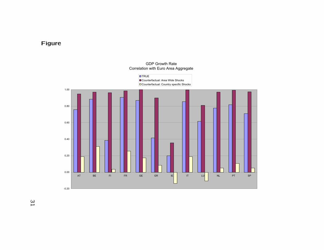
Figure
GDP Growth Rate
Correlation with Euro Area Aggregate
-0.20
0.00
0.20
0.40
0.60
0.80
1.00
AT BE FI FR GE GR IE IT LU NL PT SP
TRUE
Counterfactual: Area Wide Shocks
Counterfactual: Country specific Shocks
31
Country specific and Area wide shocks
• Counterfactuals: what would have correla-
tion been if no country specific shocks?
Answer
• correlations would have been quite high and
stable if there had been only area-wide shocks!!
=⇒ Area wide shocks progate similarly across
Euro area countries...
32
Results: Summary
• a) Idiosyncratic shocks have large effects on the gap→ correlations would have been quite high and stable ifthere had been only area-wide shocks!!
• b) Most of the fluctuations of output are due to areawide shocksExceptions are Greece, Finland, Ireland. Spain is halfway (convergence and country specific shocks!!!)
• c) Country specific shocks have large and quite per-sistent effect on the gap: they generate persistent dif-ferences across countries
Implications
→ Although small, national factors have persistent ef-fects
→ Common Euro area shocks account for the bulk ofbusiness cycle fluctuations
33

What is a reasonable benchmark?: US re-
gions
Compute the same measures...
• Use Personal Income
Remark since we use Personal Income we over-
estimate similarities across US regions.
34
Levels
STEP 1: Look at levels of Income
Define
yit ×100 log of real per-capita Personal Income
of region i in year t (PPP adjusted).
gapit = yi
t − yUSt : percentage deviation of real
Income per-capita of region i from US ag-
gregate.
35

US regions
New England NEMideast MEGreat Lakes GLPlains PLSoutheast SESouthwest SWRocky Mountain RMFar West FW
36
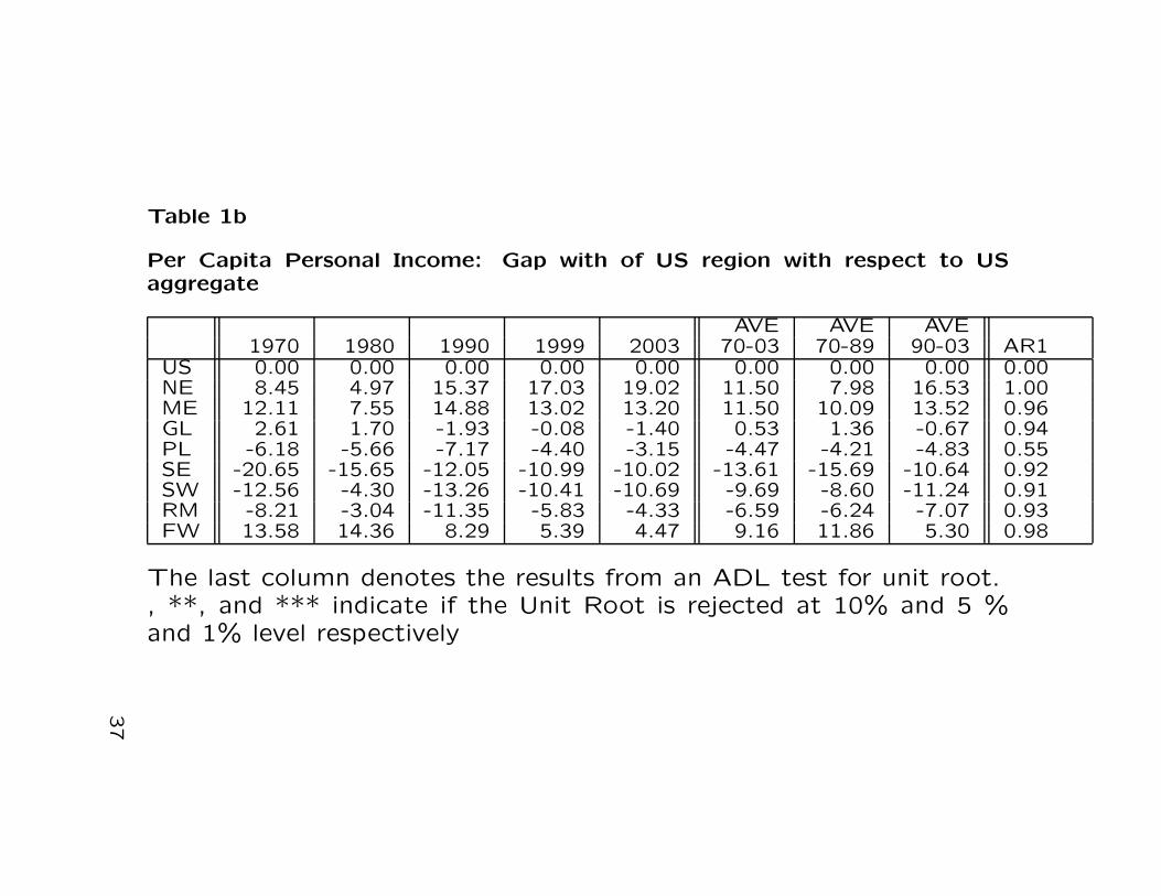
Table 1b
Per Capita Personal Income: Gap with of US region with respect to USaggregate
AVE AVE AVE1970 1980 1990 1999 2003 70-03 70-89 90-03 AR1
US 0.00 0.00 0.00 0.00 0.00 0.00 0.00 0.00 0.00NE 8.45 4.97 15.37 17.03 19.02 11.50 7.98 16.53 1.00ME 12.11 7.55 14.88 13.02 13.20 11.50 10.09 13.52 0.96GL 2.61 1.70 -1.93 -0.08 -1.40 0.53 1.36 -0.67 0.94PL -6.18 -5.66 -7.17 -4.40 -3.15 -4.47 -4.21 -4.83 0.55SE -20.65 -15.65 -12.05 -10.99 -10.02 -13.61 -15.69 -10.64 0.92SW -12.56 -4.30 -13.26 -10.41 -10.69 -9.69 -8.60 -11.24 0.91RM -8.21 -3.04 -11.35 -5.83 -4.33 -6.59 -6.24 -7.07 0.93FW 13.58 14.36 8.29 5.39 4.47 9.16 11.86 5.30 0.98
The last column denotes the results from an ADL test for unit root., **, and *** indicate if the Unit Root is rejected at 10% and 5 %and 1% level respectively
37
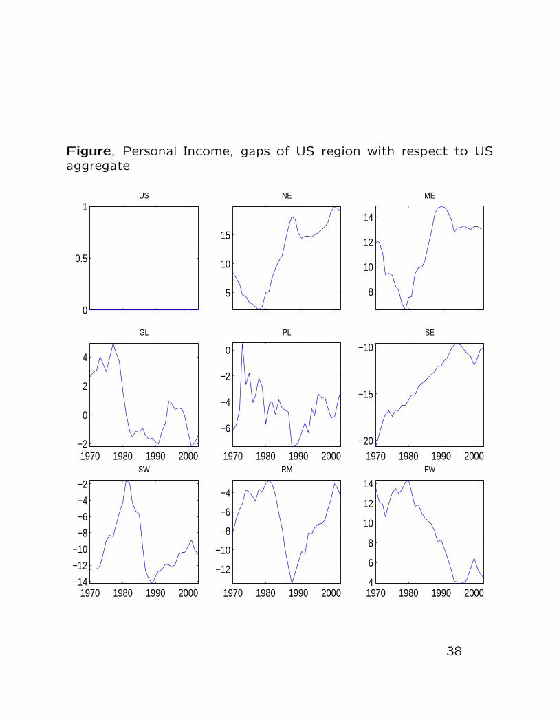
Figure, Personal Income, gaps of US region with respect to USaggregate
0
0.5
1US
5
10
15
NE
8
10
12
14
ME
1970 1980 1990 2000−2
0
2
4
GL
1970 1980 1990 2000
−6
−4
−2
0
PL
1970 1980 1990 2000−20
−15
−10
SE
1970 1980 1990 2000−14
−12
−10
−8
−6
−4
−2
SW
1970 1980 1990 2000
−12
−10
−8
−6
−4
RM
1970 1980 1990 20004
6
8
10
12
14FW
38
Comments
Gaps in the US are as persistent as those
within EMU and there is no common trend
amongst regions...
US regions do not share a common trend with
Europe while the US aggregate does!!!
39
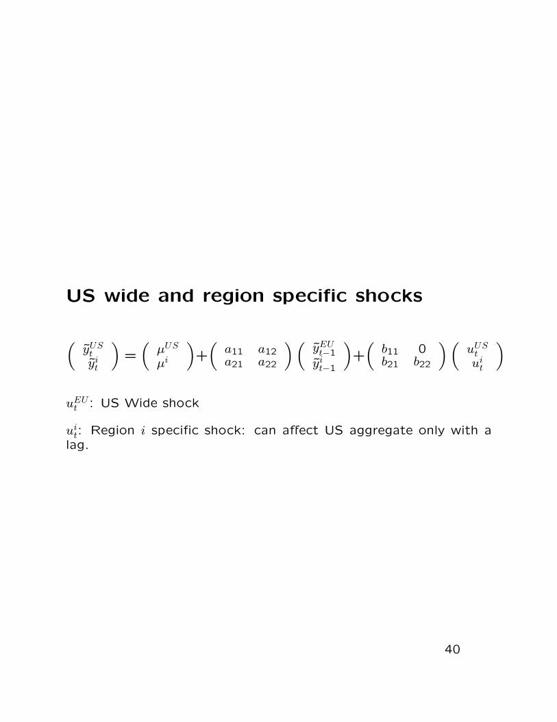
US wide and region specific shocks
(yUS
tyi
t
)=(
µUS
µi
)+(
a11 a12a21 a22
)(yEU
t−1yi
t−1
)+(
b11 0b21 b22
)(uUS
tui
t
)uEU
t : US Wide shock
uit: Region i specific shock: can affect US aggregate only with a
lag.
40
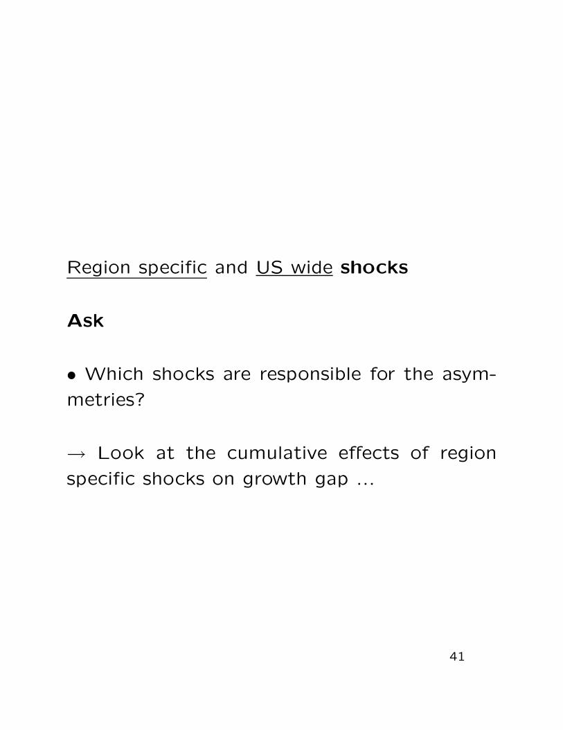
Region specific and US wide shocks
Ask
• Which shocks are responsible for the asym-
metries?
→ Look at the cumulative effects of region
specific shocks on growth gap ...
41
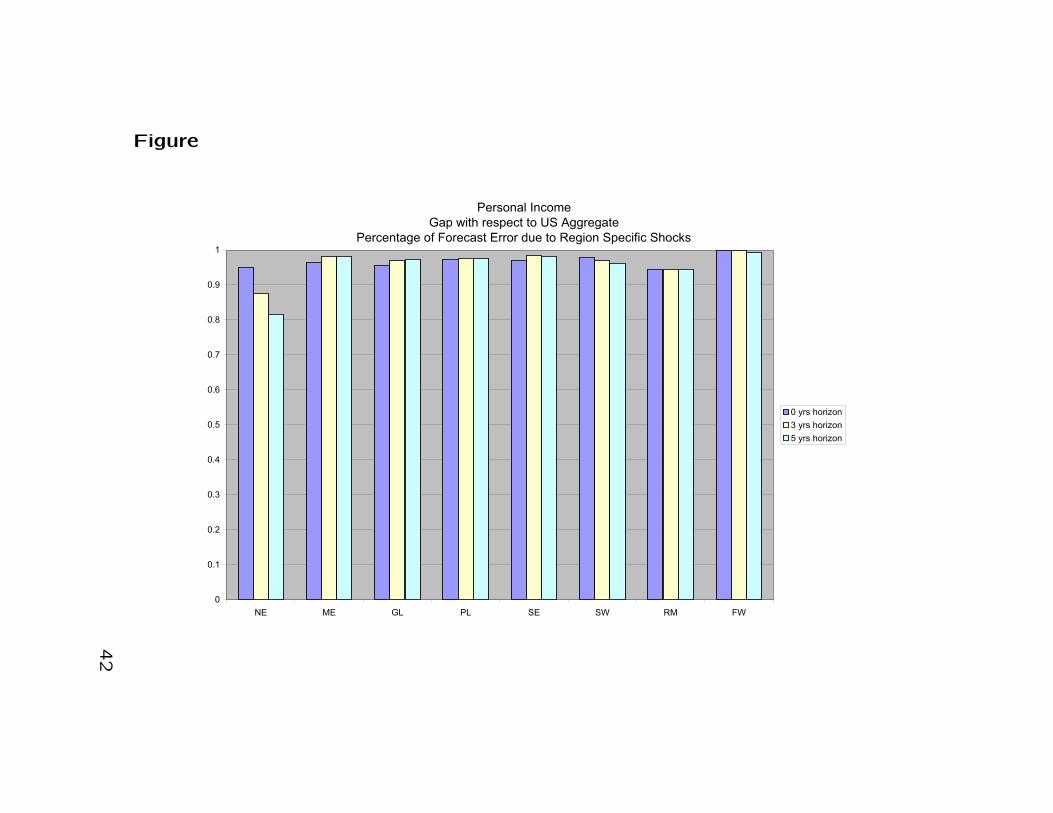
Figure
Personal Income
Gap with respect to US Aggregate
Percentage of Forecast Error due to Region Specific Shocks
0
0.1
0.2
0.3
0.4
0.5
0.6
0.7
0.8
0.9
1
NE ME GL PL SE SW RM FW
0 yrs horizon
3 yrs horizon
5 yrs horizon
42

Region specific and US wide shocks
Ask
• Which shocks are responsible for the asym-
metries?
Answer
Gap is mainly explained by region specific shocks
at all horizons
43
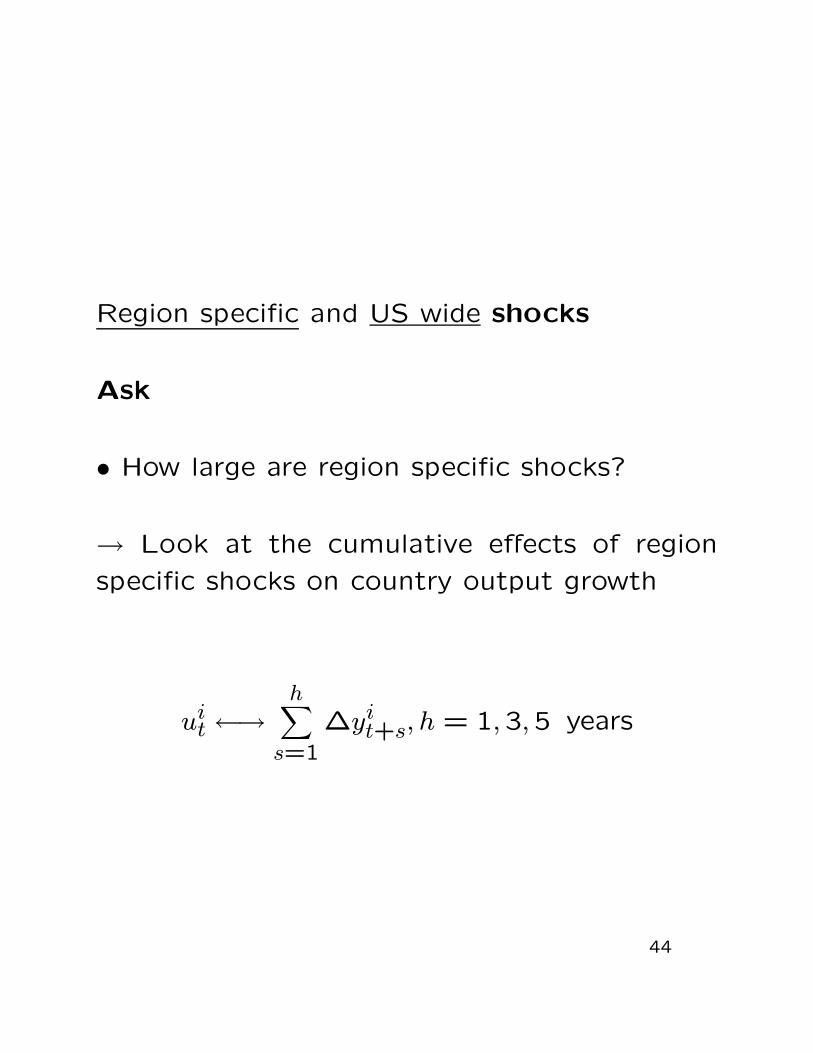
Region specific and US wide shocks
Ask
• How large are region specific shocks?
→ Look at the cumulative effects of region
specific shocks on country output growth
uit ←→
h∑s=1
∆yit+s, h = 1,3,5 years
44
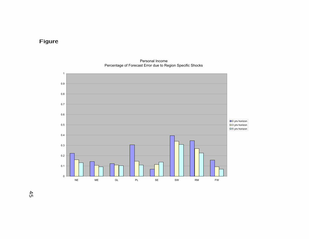
Figure
Personal Income
Percentage of Forecast Error due to Region Specific Shocks
0
0.1
0.2
0.3
0.4
0.5
0.6
0.7
0.8
0.9
1
NE ME GL PL SE SW RM FW
0 yrs horizon
3 yrs horizon
5 yrs horizon
45

Region specific and US wide shocks
Ask
• How large are region specific shocks?
Answer
• Output fluctuations yit are mainly explained
by US wide shocks at all horizons
• Region specific shocks: small + persistent
46
Region specific and US wide shocks
• Counterfactuals: what would have correla-
tion been if no region specific shocks?
47
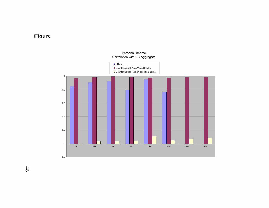
Figure
Personal Income
Correlation with US Aggregate
-0.2
0
0.2
0.4
0.6
0.8
1
NE ME GL PL SE SW RM FW
TRUE
Counterfactual: Area Wide Shocks
Counterfactual: Region specific Shocks
48
Region specific and US wide shocks
• Counterfactuals: what would have correla-
tion been if no region specific shocks?
Answer
• correlations would have been quite high and
stable if there had been only US-wide shocks!!
=⇒ US wide shocks progate similarly across
US regions ...
49

Summary
Results are similar to the core of the Euro
Area.
• Region specific shocks are small on output
and are responsible of persistent gap
• US wide shocks generate similar region spe-
cific dynamic: do not generate asymmetries
Remember since we use Personal Income we
overestimate similarities across US regions.
50
Is the common Euro shock in fact global?
→ characterize differences between the US and
the Euro area as a whole
(Giannone and Reichlin, 2005)
• Evidence on real GDP
(Not in per-capita terms following the dating
conventions...)
History of classical (level) cycles is broadly sim-
ilar
51
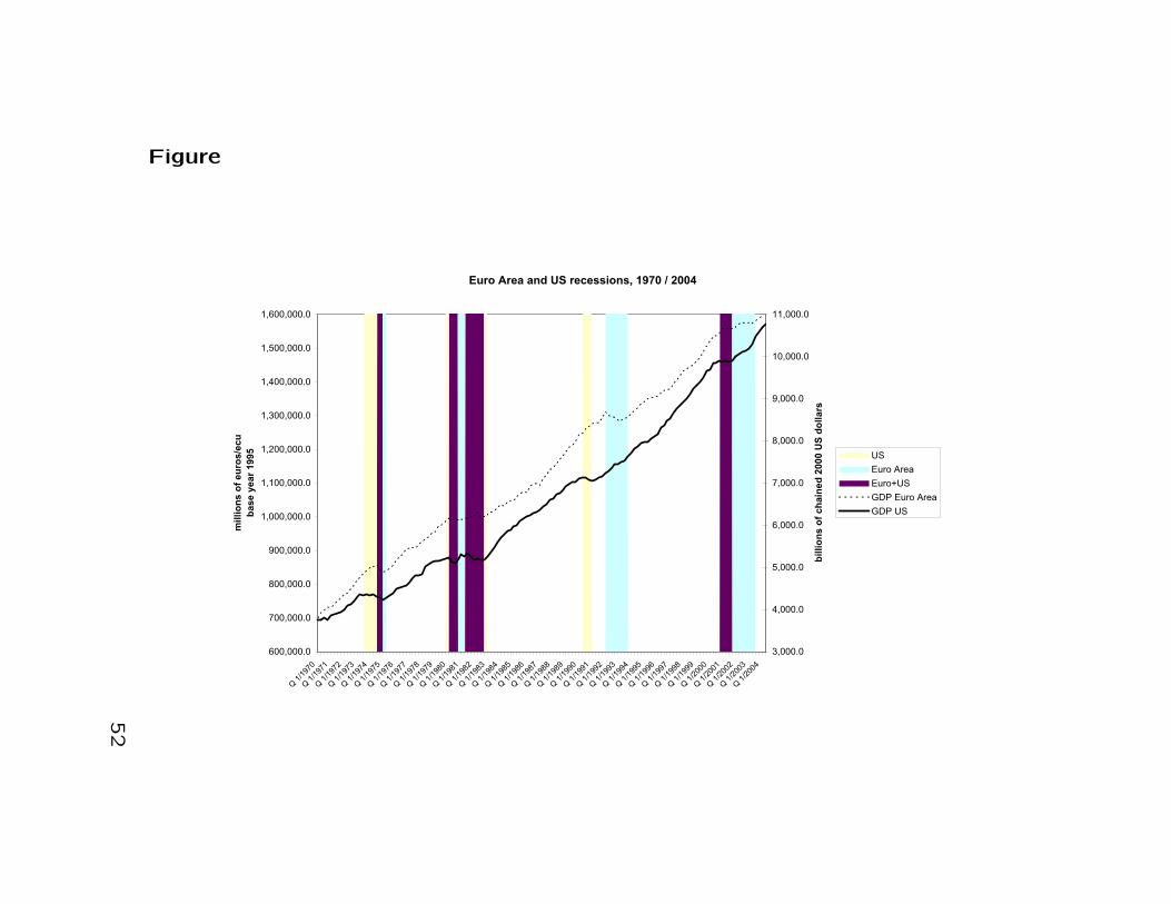
Figure
Euro Area and US recessions, 1970 / 2004
600,000.0
700,000.0
800,000.0
900,000.0
1,000,000.0
1,100,000.0
1,200,000.0
1,300,000.0
1,400,000.0
1,500,000.0
1,600,000.0
Q 1
/197
0Q
1/1
971
Q 1
/197
2Q
1/1
973
Q 1
/197
4Q
1/1
975
Q 1
/197
6Q
1/1
977
Q 1
/197
8Q
1/1
979
Q 1
/198
0Q
1/1
981
Q 1
/198
2Q
1/1
983
Q 1
/198
4Q
1/1
985
Q 1
/198
6Q
1/1
987
Q 1
/198
8Q
1/1
989
Q 1
/199
0Q
1/1
991
Q 1
/199
2Q
1/1
993
Q 1
/199
4Q
1/1
995
Q 1
/199
6Q
1/1
997
Q 1
/199
8Q
1/1
999
Q 1
/200
0Q
1/2
001
Q 1
/200
2Q
1/2
003
Q 1
/200
4
mil
lio
ns o
f eu
ros/e
cu
base y
ear
1995
3,000.0
4,000.0
5,000.0
6,000.0
7,000.0
8,000.0
9,000.0
10,000.0
11,000.0
bil
lio
ns
of
ch
ain
ed
20
00
US
do
lla
rs
US
Euro Area
Euro+US
GDP Euro Area
GDP US
52
However, differences:
1. Cycles in the US have larger amplitude and
shorter duration → GDP growth is less smooth
and less persistent.
2. They tend to lead the Euro area.
Table BC statistics
53

Business Cycle StatisticsUS Euro Area
peak to trough amplitude -0.5658 -0.2433(-0.6294) (-0.4979)
trough to peak amplitude 0.9445 0.7653(0.9589) (0.6254)
peak to trough duration 3.4000 5.3333(3.4000) (2.5000)
trough to peak duration 23.25 29(23.500) (35.00)
n. of recessions 5.00 3.00(5.00) (4.00)
Concordance Index 0.8593(0.8222)
The business cycle statistics corresponding to the NBERand CEPR dating are in bold. We show in parenthesesthe same statistics, produced by the Bry-Boschan Dat-ing Algorithm.
54

Growth cycle characteristics are rather differ-
ent
55

Euro cycle is smoother than the US cycle
(more persistent)
Variance of the growth rate of output
and of the HP trendUS Euro Area
var(∆y) 4.16 2.05var(∆HP) 0.01 0.09
var(∆HP )var(∆y) ∗ 100 .03% 4.22%
56
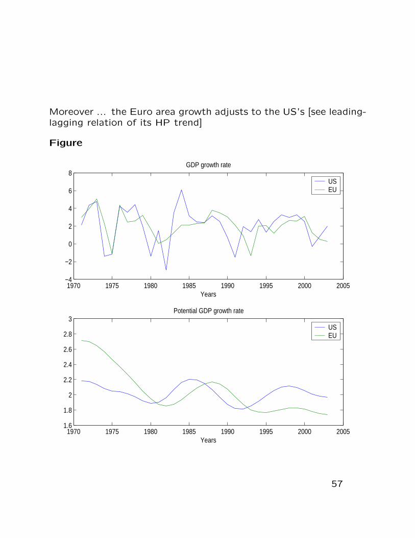
Moreover ... the Euro area growth adjusts to the US’s [see leading-lagging relation of its HP trend]
Figure
1970 1975 1980 1985 1990 1995 2000 2005−4
−2
0
2
4
6
8GDP growth rate
Years
1970 1975 1980 1985 1990 1995 2000 20051.6
1.8
2
2.2
2.4
2.6
2.8
3Potential GDP growth rate
Years
USEU
USEU
57
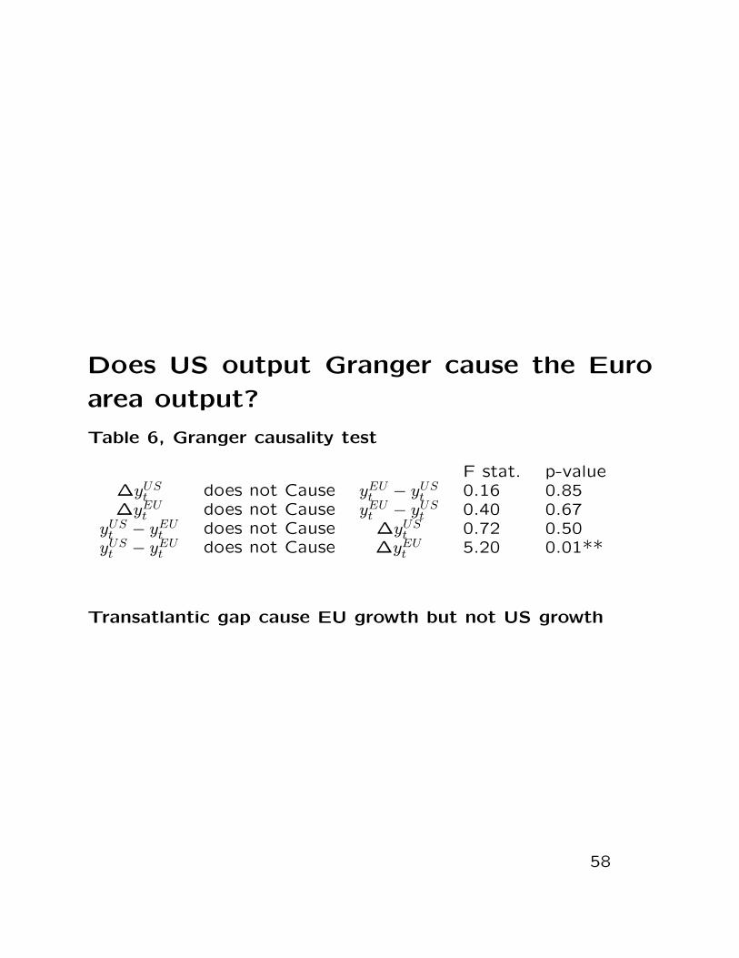
Does US output Granger cause the Euro
area output?
Table 6, Granger causality test
F stat. p-value∆yUS
t does not Cause yEUt − yUS
t 0.16 0.85∆yEU
t does not Cause yEUt − yUS
t 0.40 0.67yUS
t − yEUt does not Cause ∆yUS
t 0.72 0.50yUS
t − yEUt does not Cause ∆yEU
t 5.20 0.01**
Transatlantic gap cause EU growth but not US growth
58
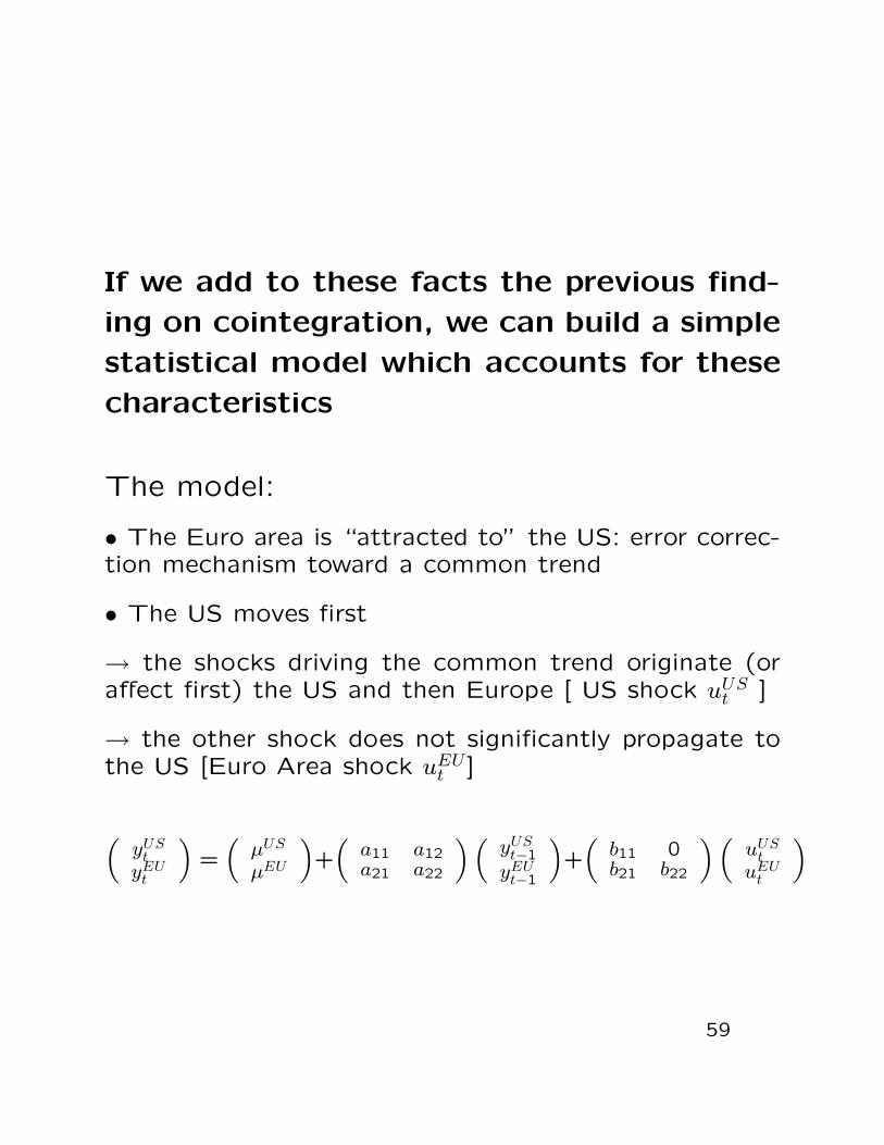
If we add to these facts the previous find-
ing on cointegration, we can build a simple
statistical model which accounts for these
characteristics
The model:
• The Euro area is “attracted to” the US: error correc-tion mechanism toward a common trend
• The US moves first
→ the shocks driving the common trend originate (oraffect first) the US and then Europe [ US shock uUS
t ]
→ the other shock does not significantly propagate tothe US [Euro Area shock uEU
t ]
(yUS
tyEU
t
)=(
µUS
µEU
)+(
a11 a12a21 a22
)(yUS
t−1yEU
t−1
)+(
b11 0b21 b22
)(uUS
tuEU
t
)
59
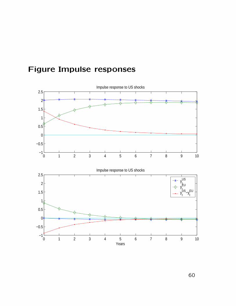
Figure Impulse responses
0 1 2 3 4 5 6 7 8 9 10−1
−0.5
0
0.5
1
1.5
2
2.5Impulse response to US shocks
0 1 2 3 4 5 6 7 8 9 10−1
−0.5
0
0.5
1
1.5
2
2.5Impulse response to US shocks
Years
ytUS
ytEU
ytUS−y
tEU
60
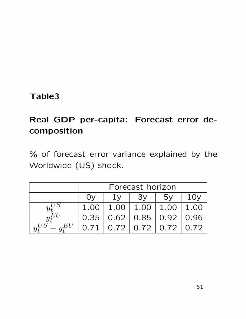
Table3
Real GDP per-capita: Forecast error de-
composition
% of forecast error variance explained by the
Worldwide (US) shock.
Forecast horizon0y 1y 3y 5y 10y
yUSt 1.00 1.00 1.00 1.00 1.00
yEUt 0.35 0.62 0.85 0.92 0.96
yUSt − yEU
t 0.71 0.72 0.72 0.72 0.72
61
Impulse response and variance decomposi-
tions
• After a worldwide shock, the US adjusts im-
mediately while Europe reacts slowly reaching
the steady state after 10 years.
• Euro Area specific shocks are very small and
transitory.
Counterfactual I
What would have the gap been if there had
only been worldwide shocks, and no Euro spe-
cific shocks?
62

Figure The Gap
1970 1975 1980 1985 1990 1995 2000 200528
29
30
31
32
33
34
35
36
37
Gap between US and Euro Area: ytUS−y
tEU
Remark
Recessions: Gap ↓
Expansions: Gap ↑
63
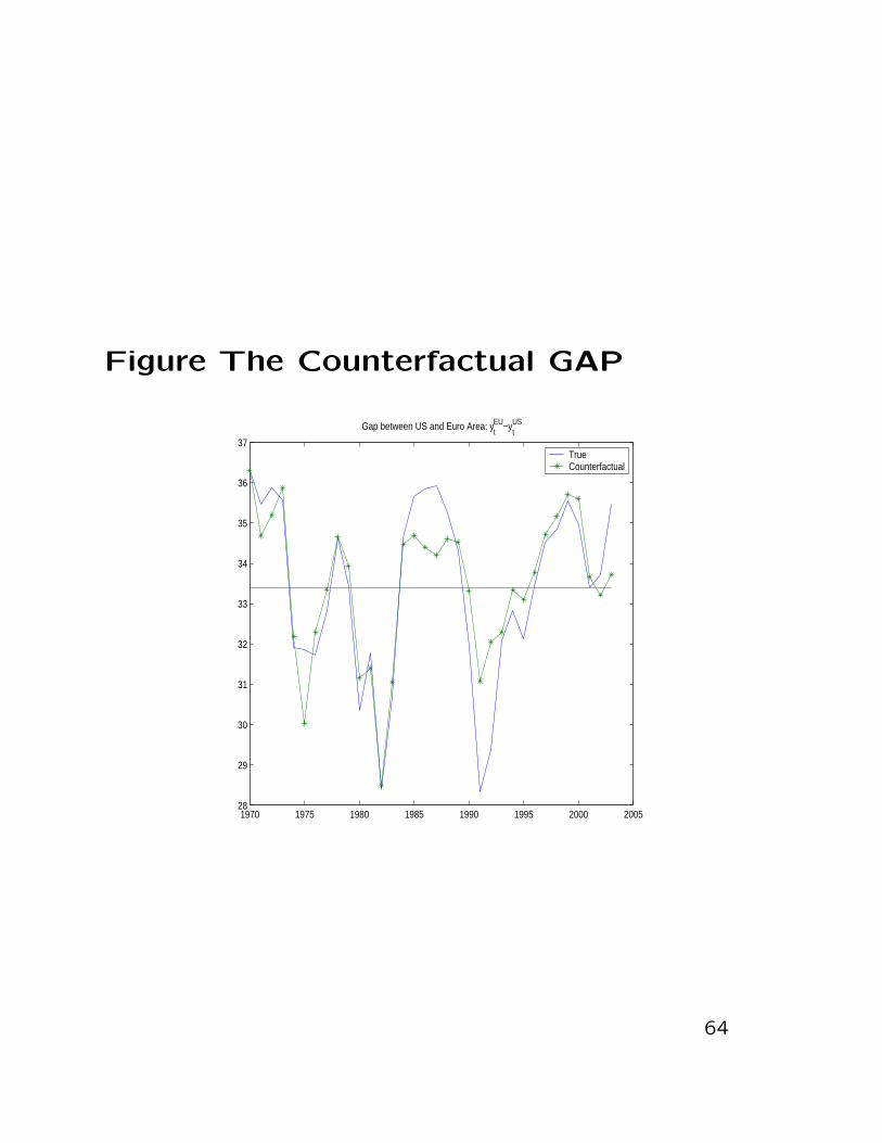
Figure The Counterfactual GAP
1970 1975 1980 1985 1990 1995 2000 200528
29
30
31
32
33
34
35
36
37
Gap between US and Euro Area: ytEU−y
tUS
TrueCounterfactual
64
Results
• The world wide shock explains most of the fluctuationsof the gap.
• During recessions, the gap tends to close since Europereacts slowly to the worldwide shock. The gap opensduring the expansions. In the middle of the cycle itreaches its maximum, but then Europe starts cachingup.
• The Euro area shock reduced the gap during the USrecession of the 1990s [German Unification]. However,the Euro area shock only postponed the European re-cession. Apart for this episode, the recent period isvery much in line with past experience (the variance ofEuropean specific shocks has not increased)
• There is a specific Euro Area cycle, which is differentfrom the US cycle because of the different propagationmechanism (qualification of Canova et al., 2003)
• Euro specific shocks are small
Conjecture/Implication :
In 2003 there were Euro Area specific forces drivingdown output.
However, accordingly to past experience these should betransitory.
65

Business cycle asymmetries and risk sharingshould we care about synchronization?
Theory: no clear prediction
a) Integration
- a1) increase risk sharing through financial market→ countries’s need to diversify as insurance againstrisk decreases → can specialize → more asymme-tries ↑(Asdrubali, Sorensen and Yosha, 1996)
- a2) faster and stronger transmission of shock(country specific, Euro wide and Global)→ less asymmetries ↓
b) common policy and monetary union:
- b1) countries cannot counterbalance country spe-cific shocks→ more asymmetries ↑- b2) countries face same policy shocks→ less asymmetries ↓
66
Evidence on risk sharing:
Sorensen and Yosha, 1999: less risk sharing in
Europe than in the US
Asdrubali, Sorensen and Yosha, 2004:
- Risk sharing through financial market has in-
crease in the last decade thanks to financial
integration
- Specialization show a tendency to increase
Here we do some of (corrected) ASY’s calcu-
lations on our data
67
Measuring risk sharing, I
ASY, 1996 and 1999 on sample 1970-2004
Define:
cit ×100 log of real individual consumption of
country i in year t (PPP adjusted).
∆h(cit − cEU
t ) = αt + βt∆h(yit − yEU
t ) + vt
∆h: h-th differences 1− Lh
βt: amount of risk not insured, percentage of
variance of GDP that is smoothed out through
capital market, credit market, transfers and fis-
cal...
Estimate βt by OLS regression.
68
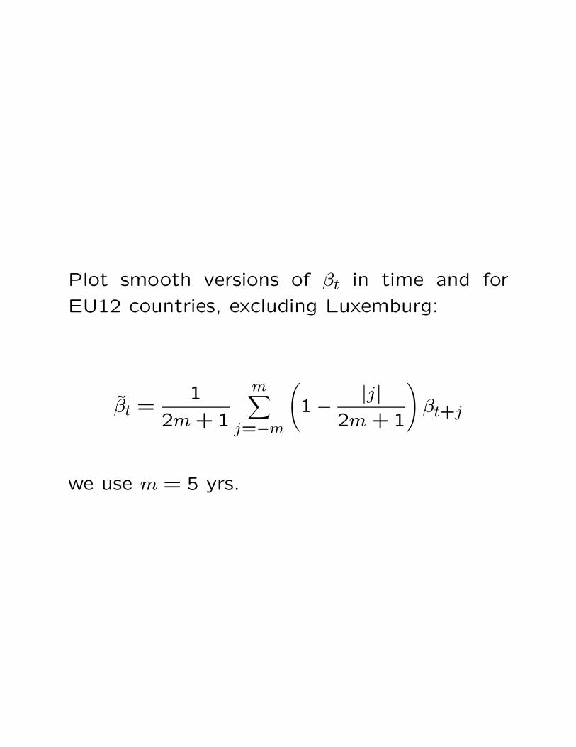
Plot smooth versions of βt in time and for
EU12 countries, excluding Luxemburg:
βt =1
2m + 1
m∑j=−m
(1− |j|
2m + 1
)βt+j
we use m = 5 yrs.
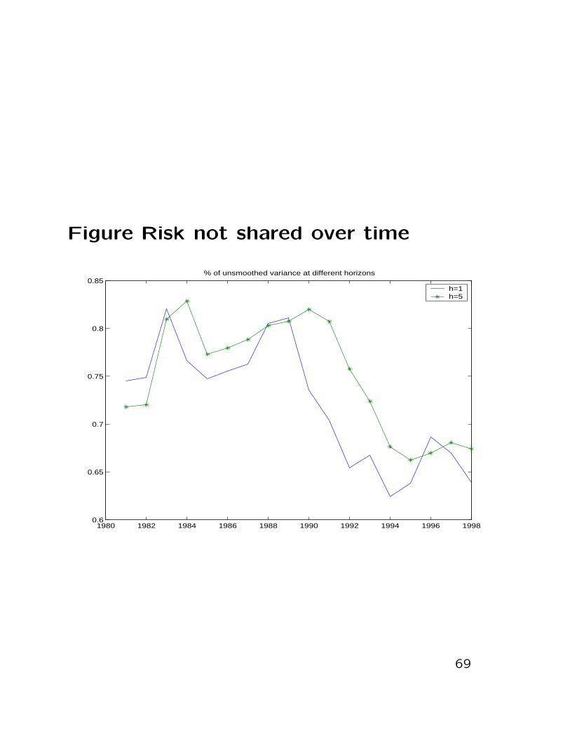
Figure Risk not shared over time
1980 1982 1984 1986 1988 1990 1992 1994 1996 19980.6
0.65
0.7
0.75
0.8
0.85% of unsmoothed variance at different horizons
h=1h=5
69

Result
Risk sharing goes up in the 90’s
70
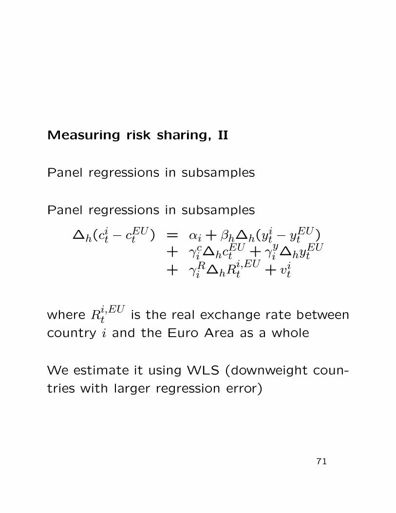
Measuring risk sharing, II
Panel regressions in subsamples
Panel regressions in subsamples
∆h(cit − cEU
t ) = αi + βh∆h(yit − yEU
t )+ γc
i∆hcEUt + γ
yi ∆hyEU
t
+ γRi ∆hR
i,EUt + vi
t
where Ri,EUt is the real exchange rate between
country i and the Euro Area as a whole
We estimate it using WLS (downweight coun-
tries with larger regression error)
71
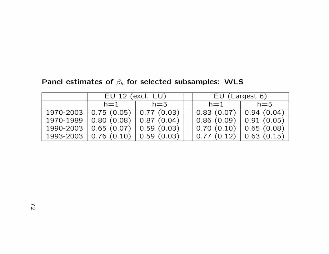
Panel estimates of βh for selected subsamples: WLS
EU 12 (excl. LU) EU (Largest 6)h=1 h=5 h=1 h=5
1970-2003 0.75 (0.05) 0.77 (0.03) 0.83 (0.07) 0.94 (0.04)1970-1989 0.80 (0.08) 0.87 (0.04) 0.86 (0.09) 0.91 (0.05)1990-2003 0.65 (0.07) 0.59 (0.03) 0.70 (0.10) 0.65 (0.08)1993-2003 0.76 (0.10) 0.59 (0.03) 0.77 (0.12) 0.63 (0.15)
72
Results
Risk sharing has increased in the last decade.
The increase is particularly strong at long hori-
zons
→ increased the ability of countries to smooth
persistent shocks to output.
Integration is working and we should care less
than before about asymmetries in output...
73
Conclusions
• If we look at output correlations from an
historical perspective, it is business as usual:
Differences between Euro countries levels of
activity are persistent, but recessions and ex-
pansions are synchronized [same as in the US]
• Euro area countries share certain common
characteristics and although they move with
the US in the long-run, the characteristics of
the Euro cycle are different than the US (it
lags, it is more persistence, it is less volatile)
• Risk sharing within the Euro area has in-
creased since the early 1990s
74


![[Lezione di Giuseppe Giannone aprile 2009] - slide della lezione](https://img.dokumen.tips/doc/110x75/586650fb1a28abd75a8d48da/lezione-di-giuseppe-giannone-aprile-2009-slide-della-lezione.jpg)