Does Vertical Integration Decrease Prices?

Evidence from the Paramount Antitrust Case of 1948

Ricard Gil∗

Johns Hopkins Carey Business School

November 2011

Abstract

I empirically examine the impact of the 1948 Paramount antitrust case on ticket prices using a

unique data set collected from Variety magazine issues between 1945 and 1955. With weekly movie

theater information on prices, revenues and theater ownership for an unbalanced panel of 393 theaters

located in 26 different metropolitan areas, I find evidence consistent with Spengler’s (1950) prediction

that vertical integration lowers prices through the elimination of double-marginalization. My results

show that vertically integrated theaters charged lower prices and sold more admission tickets than non-

vertically integrated theaters. I also find that the rate at which prices increased in theaters were slower

before vertical separation than it was after separation. A back of the envelope calculation suggests

that losses in consumer surplus due to the Supreme Court resolution and the corresponding sale of

theater holdings by Paramount and seven other companies were sizable.

∗This paper benefitted from discussions with Heski Bar-Isaac and Liran Einav as well as comments from seminar and

conference participants at ISNIE - Stanford, Universitat de Barcelona, UC-Santa Cruz and MIT. Joe Cook and Susan Van

Loon provided supreme research assistance for this project. The usual disclaimer applies.

1

1 Introduction

Understanding the impact of the organization of production is a central topic in Economics. Aside

from Adam Smith’s description of the internal organization of pin factories, many consider the

seminal work of Coase (1937) as the starting point of a literature that was later followed and

extended by a number of theories such as transaction cost economics (Williamson, 1975 and 1985;

Klein, Crawford and Alchian, 1978), property rights (Grossman and Hart, 1986; Hart and Moore,

1990; Hart, 1995), incentive-based theories (Holmstrom and Milgrom, 1991 and 1994) and post-

adaptation theories (Simon, 1951; Baker, Gibbons and Murphy, 2002). Despite this wide range of

theories and different approaches to this question, the empirical literature in this field has been

dwarfed and is lacking to support and test existing theoretical predictions (Lafontaine and Slade,

2007). Therefore, the contribution of this paper is to further the understanding of the impact

of vertical integration by documenting differences in performance between integrated and non-

integrated theaters in the US between 1945 and 1955.

This exercise should be of interest to economists in different fields but in particular to those

in organizational economics, industrial organization and antitrust policy for three main reasons.

First, in 1948 the US Supreme Court determined in the antitrust case of US vs. Paramount that

Paramount and seven others were forbidden to use bundling and other clauses that restrained com-

petition in the studio and exhibition market, as well as forced to sell the bulk of their theater

branches (only Paramount, RKO, Warner Bros., Fox and MGM owned theaters out of the eight

studios involved in the actual case). The latter part of the ruling represents an unprecedented

opportunity to examine the changes in economic performance due to an exogenous change in orga-

nizational form as the empirical literature in organizational economics suffers of pervasive problems

of endogeneity, spurious correlations and reverse causality.

A second reason why the empirical results in this paper should be of interest is the significance

of the implications of my findings for antitrust policy design. FTC and Department of Justice have

recommended in the past to break up firms charged with abuse of market power into several units

as a solution to their corresponding antitrust case. Examples of these are the Standard Oil case

of 1911 and the AT&T case of 1982 as well as the preliminary sentence of the relatively recent

Microsoft sentence in 2000. This paper provides micro-evidence (at the theater level) of the impact

of this type of sentence in economic performance and therefore helps policy makers design and

apply better policies in future antitrust cases of similar characteristics.

The third and final reason is that Spengler (1950), one of the most influential papers in industrial

economics, has its origin in the empirical setting studied here. Spengler argued that while horizontal

2

integration may increase prices and lower welfare, vertical integration may actually decrease prices

and increase welfare through the elimination of double-marginalization. Therefore, antitrust policy

should not rule against all types of integration and focus in discouraging horizontal integration.

While this applies to many industries, Spengler was inspired by the US vs. Paramount antitrust

case. Therefore, this paper provides empirical evidence on the empirical setting that motivated the

first empirical prediction of the impact of vertical integration on prices and double-marginalization.

In summary, this paper empirically examines the impact of the Supreme Court ruling on movie

theater ticket prices in the US versus Paramount antitrust case where Paramount and seven other

studios were accused of using their market power to prevent entry in movie production and dis-

tribution through movie bundling and vertical integration in movie exhibition. After a number

of appeals at lower level courts, the Supreme Court mandated in 1948 that Paramount and the

other studios to sell up to 50% of their theater holding in the US and stop movie bundling. This

paper uses the exogenous vertical separation of movie theaters mandated by the Supreme Court

to investigate the impact of vertical integration on economic performance and movie ticket prices.

In particular, I empirically explore whether theaters that were once vertically integrated had lower

prices than independent theaters before and after the Supreme Court sentence in 1948. Following

Spengler’s predictions, this decrease in prices should come along with an increase in quantity and

an increase in consumer surplus and welfare.

For this purpose, I use a new and unique data set collected from old issues of Variety (a

specialized movie industry trade magazine) edited between January 3rd of 1945 and December

28th of 1955. This data set provides weekly movie theater information on prices, revenues and

theater ownership for a sample of roughly 400 theaters located in 26 different metropolitan areas

in the US. The high frequency of the data allows me to control by city, year and theater fixed

effects while focusing on changes in price, movie receipts and admission sales before and after

the change in theater vertical structure due to the Paramount decree. I also complement these

data with information from other sources that provide information on the number of screens of

most theaters in my data set (from a website named cinematreasures.com), on the introduction of

television (Gentzkow, 2006) and on the city level theater market concentration (Movie Yearbook

issues between 1945 and 1955).

In the end, the data for this paper contains roughly 143,000 observations at the movie, theater

and week level. A result that comes from simple observation of the data is that most theaters

offered double programming (two or more within a week) and uniform pricing across movies and

weeks within a theater was the rule (contrary to what is stated in the literature). For this reason, I

collapse the data at the theater and week level for most of the empirical section below and therefore

3

end up working with almost 107,000 observations. This is far more data and variation than utilized

in most papers that have previously examined the aftermath of this antitrust case. Therefore, and

taking the limitations of the data into account, I offer both cross-sectional estimates and within-

theater before-after estimates of the impact of vertical disintegration on movie ticket prices and

theater revenues and admissions.

The cross-sectional results suggest that vertically integrated theaters sold their tickets at lower

prices than non-integrated theaters both when considering evening shows and matinee prices. Con-

sequently, integrated theaters sold more admission tickets and collected higher revenues even after

controlling for size differences. The before-and-after estimates that exploit variation in prices within

theaters show a slightly different result and yet similar in spirit. First, the data show that inte-

grated theaters did not experience an immediate increase in prices once they became non-integrated.

Second, integrated theaters increased prices at lower rates than non-integrated theaters but they

increased prices at faster rates after separating from their parent studios than theaters that were

always non-integrated. These results are similar for both evening and matinee prices. Contrary to

cross-sectional results, admissions and tickets did not go down at different rates for integrated and

non-integrated theaters after separation. After dropping observations polluted by measurement

error, I offer some evidence that revenues of integrated theaters decreased at faster rates than those

of non-integrated although they started at higher rates.

I also provide evidence at the movie, theater and week level and find similar results to those

provided with the data at the theater-week level. I find that integrated theater post lower ticket

prices and that their prices do not change whenever showing a movie distributed by other studios.

If anything, I find robust results that movies distributed by integrated studios sell at lower ticket

prices regardless of who owns the movie theater where they are showing. This suggests that even

after vertical disintegration major studios would still contract with theaters that charged low prices

as a way to deal with double-marginalization and escape high prices.

Finally, I also estimate logit demand and price sensitivity taking advantage of rich variation in

movie programming across theaters, cities and weeks. My estimates are very similar to those of

Davis (2006) but given the low prices of over 60 years ago the implied elasticities range between 0.45

and 0.75. Given these and my reduced-form results, the change in organizational form increased

prices 10% over five years (in excess to what they would have increased). That would diminish

attendance by 4.5% to 7.5% on average aside from the increase competition from television and

the alleged change in movie quality. Although it is difficult to quantify social welfare since I have

no theater cost information available, it is easy to see that consumer welfare clearly went down as

a result.

4

Given the importance of the Paramount case, this is obviously not the only empirical study

offering evidence on the aftermath of the Supreme Court ruling on this instance. Whitney (1955)

was the first to analyze the aftermath and impact of the Paramount case through a number of

interviews with industry practitioners. He notes that the impact in supply may have increased

quality but also increased prices leaving the net effect on consumers ambiguous. This case also

inspired several studies of bundling and its consequences such as Kenney and Klein (1983 and

2000) as well as Hanssen (2000). More recently, others such as De Vany (2004) and coauthors

have investigated the effect of the case by looking at the impact on market stock values, among

other dimensions, and found that the case had no effect on firm’s profits. While researching the

uniform pricing practices in the movie-theater industry, Orbach and Einav (2007) argue that the

resolution of the case restrained pricing practices in this industry. Gil (2008), not the author of

this paper, investigated the legal standing of the antitrust case while focusing on the relevance of

minimum pricing clauses and their anticompetitive consequences for the motion picture industry.

Finally, the two papers that are closer to my paper here are perhaps Hanssen (2010) and Silver

(2010). While the former argues that studios vertically integrated into exhibition to implement a

sustainable collusive agreement that would favor each other’s movies screenings, the latter explores

the impact of the vertical separation of theaters on movie production using historical data and finds

that ticket prices were unaffected by the Paramount case and that, if anything, larger transaction

costs diminished total surplus in this industry beyond potential gains in consumer surplus. This

paper contributes to this literature by exploring a long unbalanced panel data set at the theater

level and therefore answering questions that previously were only explored with aggregate and more

time concentrated data.

The empirical contribution of this paper differs from those of others and my own previous work

in two ways. On one hand, many others have studied the impact of vertical integration on prices

as a way to finding out whether vertical integration affects outcomes through lower costs or higher

productivity. Recent examples of this literature are Hastings and Gilbert (2005) and Hortacsu

and Syverson (2007). While the former examines the effect of vertical integration on gasoline

pricing in California finding a positive correlation between vertical integration and wholesale pricing,

the latter paper investigates the effect of vertical integration on prices in the cement and ready-

mixed concrete industry and finds that prices fall and quantities rise when markets become more

integrated. Hortacsu and Syverson (2007) interpret their results as an increase in productivity due

to a more efficient use of logistics for larger and vertically integrated firms in these industries. My

paper explores the relation between vertical integration and prices in a setting where improvements

on productivity are unlikely and therefore the increase in prices after vertical separation must come

5

from the emergence of a double mark-up.

On the other hand, my own previous work has examined related topics. In particular, Gil (2010)

examines the empirical relation between movie characteristics and vertical integration at the studio

level between 1940 and 1960 finding that the Paramount case decreased the number of movies

produced by studios, increase the duration of movies and increased the number of coproductions in

the industry. Gil (2009) explored the impact of vertical integration in the Spanish movie industry

and found that integrated theaters show their movies longer than non-integrated theaters and that

integrated distributors are more likely to distribute movies of more uncertain performance. This

paper adds to my previous work in that I can answer more directly the question of how vertical

separation (integration) affects consumer surplus as the data allows for theater level variation in

prices and organizational form during a time when price uniformity across theaters was not the

norm.

The remainder of the paper is organized as follows. The next section describes the institutional

details and contracting practices surrounding the Paramount antitrust case and it describes the data

collected and used in the paper. Section 3 presents a simplified version of the model in Spengler

(1950) using revenue-sharing contracts between distributors and exhibitors and provides testable

implications. Section 4 shows reduced form results of the impact of vertical integration on ticket

prices, admissions and box office revenues as well as providing robustness checks using variation at

the movie and theater level. Section 5 estimates a simple logit demand model and provides back

of the envelope calculations using implications from the previous reduced form results. Finally,

section 6 concludes.

2 Institutional Details and Data Description

This section describes institutional detail around the 1948 Paramount antitrust case. Before that,

let me describe the agents that are relevant to the case. This industry is mainly composed by

three types of agents: producing studios, distributors and exhibitors. Studios produce movies and

solve coordination problems between all agents involved in production, from directors to producers

passing through script writers and acting casts. Movie distributors are those agents that serve as

intermediaries between studios and exhibitors as they receive movies from the former and deliver

them to the latter. Finally, exhibitors own theaters that play movies provided by distributors and

sell admission tickets to viewers.

The incentives driving actions of these agents are not providing a conflict of interest between

studios and distributors as they both benefit from higher revenues from the movies, but they are

6

in conflict with the incentives of theaters. It is important to note that during the period of analy-

sis there were no ancillary markets such as DVD sales or TV markets (television audiences were

just developing at that stage). Therefore the main conflict of interest between theaters and stu-

dios/distributors were the incentives to cut the run length of movies too short (from the studio

perspective) and increasing audience turnover through high admission prices and increasing rev-

enues from the theaters’ concession stands. Since ancillary markets did not exist, all three agents

made their living out of the box of revenues collected at theaters. This made control over theater

actions more important than what it is nowadays.

2.1 Contractual Environment

Following one of the worst years for Hollywood, the Department of Justice filed suit against Para-

mount Pictures and seven others: Warner Bros., MGM, RKO, Fox, Columbia, Universal and United

Artists. The decision of filing suit came after the independent “Snow White” was the great winner

of the Academy Awards in 1938 and a feeling emerged that big movie studios were using their size

and market power to cut in quality while preserving their number of showings.1

The Department of Justice accused the defendants of restraint of trade through three main

points. First, the use of block booking and blind bidding to assure marketing their movies and

limit entry by independent studios. Second, the use of their own theater branches to gain market

power in the theater market. Third, and finally, they were accused of colluding among them to

drive out of business other studios and other exhibitors. The accusations, and therefore potential

penalties, were targeting two different groups of studios. On one end, there were the five majors that

owned production, distribution and exhibition (Paramount, Warner Bros., Fox, MGM and RKO)

and on the other side, there were the three minors (Columbia, Universal and United Artists) that

only owned production and distribution. The former group was subject to all three accusations,

while the latter was only accused of block booking and blind bidding.

Given the difference in stakes, the big five rushed in 1940 to negotiate a decree with the Depart-

ment of Justice according to which they would be able to keep their theater divisions but would

renounce to the use of block booking and blind bidding together with other contractual practices.

The only condition was that the three minors had to sign this decree as well by 1942. As the

three minors did not own theaters and relied mainly in the contractual practices under scrutiny,

Columbia and Universal failed to sign the decree within the deadline. As a result, the case was

reopened and taken to court in 1945. At this time, the studios could not hide behind the state

1Coincidentally, 1939 left one of the best vintages in motion picture history with pieces such as “Gone with the

Wind” and “Wuthering Heights.”

7

of the economy as this was booming after the war (1946 is a historical record in admission tickets

sold). Instead, the studios claimed that the demand overseas was weak at that point (Europe was

under reconstruction after World War II).2 These arguments were not convincing enough for the

Department of Justice and in 1946 the New York District Court ruled against the studios and

banned bundling as well as other contractual practices but allowed the five majors to keep their

theater branches.

The ruling did not satisfy any of the parts involved in the case and both the plaintiff and

defendants decided to appeal to the Supreme Court. After a round of appeal, in 1948 the Supreme

Court ruled against the studios and decided not only to ban bundling but also to force the vertical

separation of theaters from the five majors. After that, the case went back to the New York District

Court for confirmation while the Supreme Court encouraged the eight defendants to sign a decree

and save millions in legal fees as the case could go on for much longer. The New York District

Court confirmed the sentence by the Supreme Court and therefore the defendants proceeded to

sign the second decree.

2.1.1 The Aftermath of the Paramount Case

After the sentence was confirmed, the three minors were resigned to abandon block booking and

blind bidding practices as well as other vertical restrictions included in their distribution contracts.

This same resignation did not take place among the big five studios whom, for the most part,

decided to fight to keep their theater branches. And so different rounds of negotiations started

between the five majors and the Department of Justice to save their respective asset holdings in

the exhibition market.

The first of the five to sign the Paramount decree was RKO in December of 1948. Howard Hughes

was the owner of RKO by then and saw through the Paramount decree a way to level competition

with the other four majors since RKO was the smallest of all five studios. Therefore by agreeing

immediately (December 31st 1948) and signing the Paramount decree, Hughes was looking for a

rapid institutionalization of the Supreme Court ruling. Despite this, the actual divestiture of RKO

theaters did not occur until two years later in December of 1950 when the RKO Theater Company

spun off from RKO pictures.

Paramount followed RKO shortly after signing the decree in December of 1949. It differed

from RKO in that it immediately spun off its theater holdings from the Balaban and Katz theater

2Surprisingly enough, there was no mention at any given point of the introduction of television as potential source

of competition.

8

divisions and grouping all other theaters into the United Paramount Theaters company. Paramount

had started investing in the flourishing TV industry and, if convicted in the Paramount case, it may

have been prohibited from owning interests in other vertically related media industries. Paramount

identified the potential losses of continuing the ongoing litigation process and decided to sign the

decree and not delay any longer the separation from its theatrical divisions.

Not much later Warner Bros. and Fox signed the decree in 1951 but, similarly to RKO, they

did not separate from their theater branches until 1953. Warner Bros. named its theater division

Stanley Warner Corporation and Fox named its Fox National Theaters. Finally, Loew’s theaters

that had acquired MGM earlier (the only case of backward integration among the five majors) signed

the decree in 1954 and spun off the MGM studios from Loew’s theaters. The vertical separation of

MGM theaters was slightly more complex than other studios’ as MGM had developed a number of

interlocking arrangements with other exhibition companies that took five years to undo.

In short, the resolution and aftermath of the Paramount antitrust case changed completely

the organization and structure of transactions in the distribution and exhibition motion picture

industries. On the one hand, arms’ length transactions became regulated as block booking and blind

bidding became prohibited. Studios were now forced to distribute and contract their movies one

by one increasing transaction and search costs for both distributors and exhibitors and disallowing

all kinds of risk sharing across movies within studio cohort of movies. In return, this new way of

organizing transactions would increase competition between studios through the increase in studio

entry, and therefore benefit final consumers by an improvement in movie quality. On the other

hand, the case also changed (increased) the number of market transactions as it banned vertical

integration of studios and distribution into exhibition. This increased the studios’ exposure to

risk at the production stage, while decreased market power concentration in the theater market

hopefully benefitting consumer surplus through lower prices and theater entry increasing variety of

choices for final consumers.

In the end, this case left a quasi-natural experiment where firms (studios in this setting) were

forced to changed the way they organized transactions from within the firm to market transactions

and doing so at different points in time. This represents a unique opportunity to further our

understanding of the effect of vertical integration (or vertical separation) on economic outcomes

and in particular here on prices.

2.2 Data Description

In this paper, I use a unique data set with movie theater information contained in old Variety

magazine issues published between January 3rd 1945 and December 28th 1955. The resulting data

9

set of this collection effort contains weekly movie theater information for a total of 393 theaters in

26 different cities. As the number of theaters and cities changes week by week, the data set is an

unbalanced panel data set for which I offer a summary in Table 1. The end of each row offers the

total number of theaters for each city that Variety offered information. It is easy to conclude that

even though there is turnover of theaters there is also a lot of repetition in reporting which allows

this paper to exploit high frequency panel data. See also that Variety reported information on 23

cities in each one of the years in the sample and only three other cities appear only for one year

(Columbus, OH; Birmingham, AL; and, Lincoln, NE).3

Figures 1A and 1B show how Variety displayed the information in its weekly issues. The

magazine reported information on a sample of movie theaters within a sample of cities that aimed

to provide the big picture of the status of the movie industry and attendance in the US. Let us

remember that television was only starting to develop in those years and therefore Variety was

the main provider of such information in an integrated manner. For each of the theaters reported,

Variety provided information on the theater capacity, admission prices for matinees and evening

shows as well as theater ownership. Aside from the theater specific information, the publication also

contained information on the movie or movies playing in that theater, the studio that produced the

movie, the number of weeks that the movie had been playing in that theater as well as whether the

movie was a rerun and an estimate of the weekly box office of the movie theater. Finally, Variety

also provided the same information on the movies screened during the previous week. In this paper,

I use this information instead of the current week information because the revenue numbers are

more accurate than the within week reported projections.

Tables 2, 3 and 4 provide a closer view of the data for the cities of Boston, San Francisco and

New York respectively. Each one of these tables list the theaters that appeared in Variety over the

11 years covered in the sample specifying for any given years the number of weeks that information

is reported.4 The tables also note in yellow what theaters, and during what years, were owned by

studios. Therefore, these tables show that there is a substantial amount of variation in vertical

integration across and within theaters. This makes for an excellent setting to study the relation

between vertical integration and theater performance.

Overall I end with 143,200 movie/theater/week observations. Contrary to general belief in pre-

vious literature, theaters did not charge different prices for different movies and therefore theaters

showing several movies at the same time would charge the same price for all movies and for differ-

3They also offered information for a limited number of weeks for Toronto and Montreal in Canada, and London

in the UK. As this paper only focuses in the US, I leave that information out of the analysis.4As some theaters changed names during this time period, I was able to recover that information from cinema-

treasures.com and include it in the table with green color.

10

ent movies showing in different weeks. Given that uniform pricing was a spread-out practice and

that the goal of this paper is to investigate the impact of organizational form on prices, I collapse

the data to the theater/week level leaving 106,702 observations for the main part of the empirical

analysis in this paper. Figure 2 shows weekly admission prices for evening and matinee shows for

Radio City Music Hall in New York City between January of 1945 and December of 1955. It is easy

to see that despite the increase in prices over a span of 11 years the theater kept prices constant

as well over large periods of time,5 and therefore it makes sense to collapse the data at the theater

and week level for the empirical analysis below.

Variety offers no information regarding the number of screens operated by each theater. The

fact that some theaters regularly screen 2, 3 or 4 movies in a week seems to indicate that there

may exist differences in the number of screens across theaters and therefore it became imperative

to complement the data set with this information as this may translate in differences in costs that

are passed on to prices. For this reason, I looked for each theater listed in Variety in the website

www.cinematreasures.com which documents the existence and characteristics of old theaters.6 As

most theaters do not exist any longer, the information is gathered through contributions from

individuals that attended the movie theater back in the day or that are related to previous owners.

Most testimonials provide information on when a theater was rebuilt and increased its number of

screens as well as reseated to fit more or less people. Given this information, I am able to collect

and check information on the number of screens and seats during the period of time of my sample.

It is also important to highlight that during this time period television was introduced in the US

spreading quickly across cities and states to reach over 80% of US households in 1960. This event

provides a source of exogenous variation in competition faced by theaters in most cases creating exit

despite strategic considerations (Takahashi, 2011). It is useful then, before presenting summary

statistics and proceeding with the empirical analysis, to understand the kind of variation in TV

adoption as exogenous source of theater competition.

The top of Figure 5 depicts the evolution of the percentage of US households with a TV set

between 1940 and 1960. As described above, almost no households owned a TV prior to 1945 and

this percentage spiked shortly after up to near 90% by 1960. As for my sample, Table 5 provides

the year of TV introduction for all cities and markets in my data set according to Gentzkow (2006).

It is easy to conclude that bigger cities were early adopters (NYC, Chicago, LA and Washington

DC) and smaller cities were late adopters (Portland, OR, and Lincoln, NE). The bottom of Figure

5 I chose Radio City Music Hall in New York City because Variety reported prices for this theater for every week

during the 11 years I collected data for.6This website has also been used by Takahashi (2011).

11

5 displays then the cumulative population in our sample that is exposed to the introduction of

television (according to data in Table 5) and shows a striking resemblance with the top of Figure

5. Therefore it is fair to assume that theaters in my sample of cities follow a similar pattern to the

US as a whole in this regard.

I proceed in Table 6 to report summary statistics for the main variables used in this paper.

First of all, note that 61% of observations belong to theaters that at some point were owned by

a studio even though only 34% belong to theaters actually owned by studios. See then that the

average evening price is $1 but that value goes from 0.25 to 3.6 and that theaters that were ever

integrated charged on average (across cities and years) $0.007 more than independent theaters.

The average price for a matinee show is $0.59 where integrated theaters charge 0.034 less than non-

integrated theaters. On average, theaters collected $14,232 and sold 14,349 tickets while having

only one screen and 1,575 seats per screen. It appears that theaters ever integrated have the same

number of screens than non-integrated theaters, but had more seats and therefore collected higher

box office revenues and sold more tickets than non-integrated. Finally, the empirical analysis also

includes variables that measure the number of years since TV was introduced in a market and the

Hirschman-Herfindhal Index (HHI hereafter) using theater counts by theater circuit and city. It

turns out that independent theaters are located in more concentrated markets and markets that

adopted television earlier than theaters that were ever integrated.

Note that a complication from the data is that in the second half of the period Variety started

reporting information within cities in movie theater groups that charged the same admission prices

and showed the same movies. This created problems of seat capacity and revenue reporting as

seats were reported jointly and average movie theater revenues across theaters were reported. I

address the first issue by fixing the number of seats within the lifetime of a theater.7 Since I cannot

directly address the second issue, I coded up when and where joint revenue reporting takes place

and I provide robustness checks without this set of observations.

Table 7 provides summary statistics at the theater/movie/week level for those variables that

have variation at that frequency. See for example that theaters that were ever integrated showing

movies of the studio that owned them represent 18% of all 143,200 observations while a total of 15%

are from integrated theater showing movies from studios that currently own them. These data also

shows that theaters that were ever integrated showed more movies from the big five studios and

less movies from the three minors than independent theaters. Within the subsample of theaters

ever integrated, these theaters showed more movies from the big five and less from the minors when

7Reports in www.cinematreasures.com seem to indicate that reseatings and theater restructuring never changed

drastically the number of seats of a theater.

12

they were in fact integrated.

As time variation is relevant in this project, I present the evolution of the main variables of

interest across years in Table 6. Figure 3 displays yearly averages for revenues, and evening and

matinee shows admission prices as well as the share of integrated movie theaters in the sample.

It is easy to see that both evening show and matinee prices increase between 1945 and 1955 from

0.8 and 0.4 to 1.3 and 0.8 respectively. Similarly, the share of integrated theaters in the sample

starts at 60% (as large cities are overrepresented in the data) in 1945 and goes down to 0% in 1955.

Finally average reported revenues go down from almost $16,000 to barely $14,000. As I compute

admission tickets as the ratio between revenues and evening shows prices, it is easy to see that

admission ticket sales will go down more sharply than revenues given the rapid increase in prices

observed in the data.

Figure 4 shows the evolution of prices, revenues and admission tickets for independent and ever

integrated theaters. The top graph in Figure 4 shows how evening and matinee shows changed

during this period of time. If anything it is easy to see that there is almost no difference in matinee

prices across theater types while evening prices for theaters ever integrated seem to have increased

faster than those of independent theaters. The bottom graph displays box office revenues (solid line)

and admissions sold (dashed line) by theater type. Aside from theaters that were ever integrated

selling more admissions and collecting higher revenues, there does not appear to be any difference

in how these lines evolve over time according to these graph.

Despite the clear unconditional negative relation between integration and prices in the cross-

section (Figure 3) and the apparent similarities in trends over time (Figure 4), some of these are due

to compositional changes in the sample as the theaters reported by Variety changed across weeks

and years. Therefore, the empirical analysis below takes into account this and rely on within market

and within theater variation across time to estimate the relation between prices and organizational

form.

3 Revisiting Spengler’s Theoretical Framework

In this section I adapt the model of Spengler (1950) to the case of revenue sharing between upstream

and downstream non-integrated firms. As I show below, the model results in exactly the same

implications as the original paper.

13

3.1 A Model of Double-Marginalization with Revenue Sharing

Let me model the interaction between an upstream producer and a downstream retailer . Simi-

larly to Spengler (1950), the downstream retailer faces a linear demand function () = − .

Following institutional features explained above, I assume that the cost function of the upstream

producer and downstream retailer are such that () = and () = + respectively.

When upstream and downstream firms are not integrated, they split revenues using revenue sharing

contracts such that the upstream producer keeps percentage of the revenues and by default the

downstream retailer keeps 1− percentage.

I first consider the case when upstream and downstream producers are not integrated. Given

the assumptions above, the downstream retailer maximizes profits such that

max(1− )(− )−−

which yields

=−

1−2

and

=+

1−2

.

Taking this into consideration, the upstream producer problem is

max

()()−

such that

() =−

1−2

,

() =+

1−2

,

and

(1− ) ()()−()− ≥ 0.

Taking FOC, ∗ is the value that solves

2

23 − 3

2

22 + (

32

2+

2

2)+ (

2

2− 2

2) = 0

and such that 0 ∗ 1.

14

Let me now consider the case when upstream and downstream agents are integrated. In this

case, the integrated firm maximizes profits such that

max(− )−− −

and solving FOC I find that

=−

2

and

=+

2.

When comparing and with and , it is easy to show that and

for any 0 ∗ 1.

3.2 Testable Implications

The model (as Spengler’s original paper) above provides two testable implications:

• The model predicts that vertically integrated retailers will charge lower prices than non-integrated retailers ceteris paribus. Therefore, a theater will charge higher prices when going from

integrated to disintegrated.

• The previous decrease in prices also suggests that non-integrated retailers will sell less unitsthan integrated retailers ceteris paribus.

Finally, a third implication that I can evaluate with the data at hand suggests that a change

from integration to non-integration is associated with a decrease in consumer surplus ceteris paribus.

In the next section, I take these implications to the data.

4 Empirical Evidence

In this section, I first test the direct implications of the model by empirically analyzing the relation

between prices, revenues and tickets sales, and vertical integration at the theater level. I also provide

robustness checks by dropping observations with severe measurement error in revenue reporting as

well as repeating the cross-sectional analysis at the theater, movie and week level.

I leave for the following section the estimation of movie theater demand and I make “back of

the envelope” calculations on the loss of admissions due to the increase in prices associated with

the wave of disintegration in the US movie theater industry.

15

4.1 Higher prices, Lower Revenues?

To establish the empirical relation between outcomes (prices, quantities and revenues) and vertical

integration, I first run OLS regressions with the following specifications,

= 0 + 1_ + 2 + 3 + + + (1)

and

ln() = 0 + 1_ + 2 + 3+

+4_ ∗ + 5 ∗ + 6 + + + (2)

where stands for the left hand side variables in the empirical analysis (evening prices, matinee

prices, ticket admissions and box office revenues) by theater , city , week and year . I use the

first specification above to estimate cross-sectional differences, while I use the second specification to

estimate differences in changes in prices over time. Right hand side variables in the first specification

are a dummy variable _ that takes value 1 if theater in city was ever integrated

and 0 otherwise, a dummy variable that takes value 1 if theater in city is integrated

in week of year and 0 otherwise, and theater and time-varying characteristics such as

the number of screens and seats per screen at theater , the number of years since television was

introduced in market and the HHI for market in year as well as city and year fixed effects

to capture city and year specific unobservables correlated with pricing decisions at the theater

level. The second specification varies from the first one in that the dependent variable is in logs

and the independent variables include a time trend variable (week, month or year) and its

corresponding interactions with the dummies described above _ and . This

second specification also includes theater and year fixed effects.

In Table 8 I show results of running OLS regressions for specifications 1 (columns 1 to 3) and 2

(columns 4 to 6) of evening prices on the independent variables detailed above. Results in column

1 show no statistical relation between prices and integration across years and cities as it was clear

in Figure 4. In column 2 I introduce city fixed effects to account for variation across cities and

I find that theaters when integrated charge 4 cents less than independent theaters. There is no

apparent difference between prices of theaters ever integrated and independent theaters. Column

3 introduces city and year fixed effects and shows a difference of again roughly 4 cents between

integrated and independent theaters. Note that a difference in mark-up of around 4% (the average

price charged in the sample is $1) is a fairly reasonable estimate for savings due to the elimination

of double-marginalization and therefore these seem fairly plausible results.

16

This first three specifications also include controls for the number of screens and the capacity

per screen, but these appear to be statistically insignificant. Evening prices are also positively

correlated with the number of years since television was introduced in a market and negatively

correlated (if anything) with market concentration.

The second set of specifications in Table 8, columns 4 to 6, uses ln[_] as dependent

variable as well as time trends and interactions with the different organizational form dummies used

previously. I start with column 4 where I include theater and year fixed effects together with a within

year week trend named (taking values between 1 and 53) interacted with _

and dummies. Results show that prices of independent theaters within a year go up at a

weekly rate of 0.0004% and that this differs from those theaters ever integrated (0.0011%) and

those in fact integrated (0.0007%). In other words, theaters that are ever integrated increase prices

at a faster rate than independent theaters, but the former increase prices at a slower rate when

are in fact integrated. Columns 5 and 6 introduce month-year and year trends respectively. The

results in these two columns are consistent with those in column 4. Let us focus on the results of

column 6. Within the lifetime of a theater, evening prices went up on average at a yearly rate of

2.4%. Theaters that were ever integrated increased prices at almost 2% faster than other theaters,

but while integrated their prices grew as slowly as 0.4% slower than theaters that were independent

all along. If anything, the number of years since introduction of television is positively correlated

with evening prices while HHI has no statistical significance.

In summary, the results in Table 8 show that when comparing integrated and non-integrated

theaters in the cross-section within a city and week integrated theaters charged 4 cents less (4%

less) than independent theaters. When comparing changes in prices over time, this table shows

that integrated theaters increased prices 0.4% slower than independent theaters and after becoming

independent their prices increased at a rate 2.1% faster than before and 1.7% faster than theaters

that were independent all along.

Table 9 repeats the same exercise with matinee prices and find similar results. Column 1 shows

no statistical relation between vertical integration and matinee prices. If anything the number of

screens and the capacity per screen are negatively correlated with matinee prices, and the number of

years since television introduction is positively correlated with prices. In columns 2 and 3 I introduce

city and city/year fixed effects respectively. The results there show that theaters that were ever

integrated charged 4 cents less than theaters that were independent all along but these theaters did

not seem to charge statistically significant lower prices when they were in fact integrated. As in

Table 8, columns 4 to 6 use the [_] as dependent variables and week, month and

year time trends respectively with organizational forms interactions in the right hand side as well

17

as theater fixed effects. The results are similar across specifications in that all three indicate that

even though theaters that were ever integrated increased prices at a faster rate than independent

theaters, when integrated these theaters increased prices at lower rates than independent theaters.

Therefore, the results for evening shows and matinee shows prices are very similar.

In Table 10 I examine the relation between admission tickets sold and vertical integration with

the same specifications as in Table 8 and 9. It is important to note here that Admissions (tickets

sold) is measured with noise as this is the result of dividing reported revenue (rounded up or down

by Variety most of the time) by the reported evening show price (even though matinee shows

must have had positive attendance). Having this caveat in mind, the cross-sectional regressions

in columns 1 to 3 show that integrated theaters sold more tickets only when they were in fact

integrated and not after becoming independent theaters. These specifications also show that the

number of screens and capacity per screen is positively correlated with admissions sales and that

every year since TV introduction was associated with up to 800 weekly attendees less. Theaters

in more concentrated markets were also selling less tickets. Columns 4 to 6 (as in the previous

two tables) use [] as dependent variable and introduces week, month and year time

trends respectively. Interestingly enough there is no difference in decrease rates in admissions

between integrated and independent theaters.

Finally, Table 11 repeats the same exercise with weekly box office revenues per theater as depen-

dent variable. The cross-sectional results here show no difference in revenues between integrated

and independent theaters. Similarly to results in Table 10, theater size is positively correlated with

revenues and HHI is negatively correlated with revenues. Columns 4 to 6 show again that there is

no difference in revenue decay rates across theaters of different organizational forms.

In summary, the results here indicate that integrated theaters charged lower prices for evening

and matinee shows and that this practice translated into more tickets sold but no difference in box

office revenues. I also found that theaters increase prices at a slower rate when they are integrated

than after becoming independent and at slower rate than theaters that were independent all along.

4.1.1 Robustness Checks

In this section I provide two additional empirical exercises that look into how sensitive the results

are to the idiosyncrasies of the data. First I take into account the fact that Variety was jointly

reporting revenues of theaters that showed the same movies and charged the same prices within

a city and week. This joint reporting practice clearly introduces noise and therefore may tilt the

initial results towards statistical insignificance.

18

Table 12 addresses this problem by dropping all observations from cities and weeks that jointly

reported revenues. Columns 1 to 6 repeat the analysis in Table 10 using and []

as dependent variables. If anything, theaters that were ever integrated appeared to have faster

decay rates than independent theaters but this result is not robust to the use of different time

trends. Columns 7 to 12 repeat the analysis in Table 11 using __ and

[__] as dependent variables. There are no significant changes in speci-

fications 7 to 9, but columns 10 to 12 show that box office revenues decreased faster when theaters

were in fact integrated than before changing to independent.

The second robustness check that I implement is to run the same cross-sectional specifications

from Tables 8 to 11 taking as observation the movie-theater-week triad as unit of analysis while

accounting for whether the movie on screen is distributed by the same studio that owns the theater.

I show results of this exercise in Table 13 from columns 1 to 12 for Evening Price, Matinee Price,

Admissions per Movie and Box Office per Movie (I divide total admissions and box office by the

number of movies screened in a given week and theater) as dependent variables.

Columns 2 and 3 show that integrated theaters charge around 3 cents less than independent

theaters. Most importantly, columns 1 to 3 show that movies from the five majors and three minors

are screened in theaters with lower prices (4 cents lower). Not surprisingly due to uniform pricing

practices (see again Figure 2), whether an integrated theater showed a movie distributed by its

own studio did not affect prices. All other results and correlations are the same as in the original

Table 8. Columns 4 to 6 repeat the exercise with _ as dependent variable. I find

that, similarly to Table 9, that theaters that were ever integrated charged 3 cents lower prices than

independent theaters regardless of the movie screened or whether they are currently integrated.

The results in these specifications also show that, just like in columns 1 to 3, movies from the

eight studios implicated in the antitrust case are more likely to screen in theaters that charge lower

matinee prices (2 cents lower). Other results are similar to those in Table 9.

Finally, columns 7 to 12 repeat the same exercise with__ and___

These specifications show that integrated theaters sell more admission tickets and collect more rev-

enues than independent theaters even after accounting for whether the movie is distributed by a

big studio. These theaters did not seem to collect higher revenues when they screened movies of

their own studio. All other results are in line with those in Tables 10 and 11.

The results in Table 13 seem to suggest two main channels for the negative relation between

vertical relation and prices. First, integrated theaters operate at lower cost and that translates

into lower prices which then drives up admission sales regardless of the studio of the movie playing.

Second, the fact that movies from integrated studios (all eight of them) sell at lower prices than

19

movies from other studios seems to suggest that these studios were concerned with high prices and

therefore actively looked for outlets where prices were indeed lower.

5 Demand Estimation

To estimate the impact of the Paramount antitrust case resolution on attendance, I must first

estimate movie demand. Let me assume that a given consumer obtains utility if watching

movie in theater located in city during week of year . This utility then can be written

down as

= + + + + +

where is the utility derived from consuming movie , is the utility derived from consuming

any movie in theater located in city , is the disutility associated with every dollar paid in price

, is a seasonal component of demand, is the unobserved market specific demand

shock for movie in city , and is the traditional logit error specific to consumer and

movie in a given theater and period . For simplicity, I can rewrite this expression in terms

of the mean utility of movie in theater in week such that

= + .

The outside option here would be not watching any movie and therefore derive utility

0 = 0 + 0

where 0 is the mean utility of not watching a movie in city and week , and 0 is a random

logit error specific to the outside option in city and week .

Following standard results after integrating over the logit errors, the share of attendance for

movie in theater in week will be

=

1 +

X=1

20

and the share of people that chose the outside option would be

0 =1

1 +

X=1

.

Applying logs as in Berry (1994),we have that

ln()− ln(0) = + + + + .

Then if I had attendance for all theaters in all the observed cities, I could simply run OLS on

this specification implementing movie-city fixed effects or using an instrument for price that was

correlated with price and uncorrelated with movie-market specific demand shocks.

Unfortunately, I only observe a subset of theaters within a city for any given week. This prevents

me from both observing weekly total movie theater attendance and potentially the size of the outside

option. To solve this, I assume that each inhabitant in a given city is going to the movies at most

once a week and therefore the maximum attendance in a given week and city is its population.

This allows me right away to compute the market share of each one of the observed theaters. To

address the fact that I do not observe the complete set of choices available to consumers, I rely

on the use of city/week fixed effects (to proxy for (0)) following the spirit of the matching

estimator proposed by Fox (2007) and its applications.8

In the end, I run OLS regressions such as

ln() = + + + + , (3)

where are variables that vary across theaters and cities and that I eventually substitute

for city/year/week fixed effects. This fixed effect is specially important to control for ln(0) as

this varies across cities but does not within a city and specific week. Specifications also introduce

movie and theater fixed effects to control for unobservables that may be correlated with prices and

therefore bias my estimates of .

On that note, the main source of concern is the unobservable , a demand shock specific to a

movie and market match. One would think that theaters would change prices accordingly to these

movie/market specific shocks and therefore standard OLS regressions would yield biased estimates.

This is not an issue here precisely because of the uniform pricing practice that kept prices constant

8See Bajari, Fox and Ryan (2008) for an application to cellular demand estimation. Conlon and Mortimer (2011)

are also concerned with this issue, even though here I follow more closely the approach in Fox (2007).

21

regardless of the movies played in a theater. Despite that, I address this issue by introducing

movie/city/year/week fixed effects and also by instrumenting Evening Price with Matinee Price.

The fixed effect controls for the specific shock in demand for a movie in a determinate city and

therefore takes account of that correlation. The instrument is correlated with Evening Price and

more importantly is a good proxy for cost per ticket at the theater level as discounted prices tend

to be closer to average cost.

Table 14 displays results of estimating specification (3) above. See in column 1 that without

introducing any fixed effect the price coefficient is around −13. Columns 2 to 7 include theater,city, year/week and movie fixed effects yielding very similar coefficients that range between −045and −053. Finally, columns 8 and 9 introduce movie/city/year/week fixed effects to control formovie/city demand differences and find estimates that are much higher of −058 and −079. Sta-tistical significance is at 10% at best in these last two specifications which is explained by the fact

that Variety barely ever reported on the performance of a movie in more than one theater within

one city (no variation) or, when it did in the last few years, it reported jointly (measurement error).

The last three columns in Table 14 (columns 10 to 12) report estimates of instrumenting Evening

Price with Matinee Price. Column 10, as in column 1, includes no fixed effects and provides a large

price coefficient estimate of −145 while columns 11 and 12 introduce city, theater and year/weekfixed effects and provide much similar estimates with previous columns of −059 and −037. Otherresults in this table suggest that larger theaters had larger market shares and that theaters located

in early TV adopting markets and less concentrated markets had higher market shares.

In summary, the price coefficient estimates range between −037 and −079 which are verysimilar estimates to those in Davis (2006). The difference here with that study is that implied

elasticities in this sample are around −032 and −075 due to the fact that the average EveningPrice in the data is $1 while prices in Davis (2006) are substantially higher. If anything, the implied

elasticities range between −003 and −3 across all weekly theater observations and they grew overtime on average, larger theaters being more elastic than smaller theaters. With these numbers in

mind and taking into account (Table 8) that in a period of 5 years after vertical separation theaters

ever integrated increased prices 10% faster than otherwise, this means that theater attendance in

theaters previously owned by studios decreased by between 3.2% and 7.5% faster than otherwise

due to the increase in prices caused by the aftermath of the paramount decree.

Given this back-of-the-envelope calculation and taking into account that on average theaters

that were ever integrated collected close to $16,600 a week, the impact on welfare of the vertical

separation for a theater owned by a studio before 1948 and five years down the road is approximately

between $500 and $1,200 per week and therefore between $26,000 and $60,000 a year. This is

22

indicative of a lower bound of the impact of the antitrust case sentence on consumer surplus and

welfare in an individual theater basis. Given that De Vany (2004) and coauthors find no effect on

studio profits (no effect in stock market prices), it must be then that all effect was concentrated in

a decrease in consumer surplus of at least $26,000 a year per theater affected.

6 Concluding Remarks

This paper empirically estimates the impact of the 1948 Supreme Court decree in the US vs.

Paramount antitrust case on movie ticket prices, admissions and box office revenues. After several

years of litigation and appeals, the Supreme Court mandated the eight largest studios in the US to

stop bundling practices and to sell the bulk of their theatrical divisions. As a result, an econometric

study of the impact of such judiciary resolution represents a unique opportunity to study the effect

of vertical integration on performance measures such as prices, sales and revenues.

Aside from the intellectual value of the research question, this study is also valuable in that the

Paramount case is one of the largest and most important cases in US antitrust history and therefore

understanding the ultimate consequences of its resolution is key for future antitrust policy design.

In particular, this case is among the few (together with the Standard Oil case of 1911 and the

AT&T case of 1982) where antitrust authorities requested to break up firms under scrutiny. This

type of sentence is not free of huge transaction and reorganization costs on the firm’s side and it is

therefore important to know their consequences on outcomes to evaluate the benefits and costs of

such policies. This paper attempts to do so by exploring the impact of mandated vertical separation

at the theater level in the 1948 Paramount antitrust case.

My empirical findings show that integrated theaters charged 4 cents less for evening shows on

average than independent theaters and that these charged the same prices after becoming inde-

pendent. I also find that theaters that were ever integrated charged 4 cents lower for matinee

shows regardless of whether they were in fact integrated at the time. More importantly, integrated

theaters increased their prices (both evening and matinee prices) over time at slower rates than

independent theaters and increased prices much faster after becoming independent. Other results

suggest that even though integrated theaters sold more admission tickets and collected more rev-

enues than independent theaters, there was no difference in the rate at which sales and revenues

decreased across theaters of different organizational forms. These findings are robust to different

specifications and checks implemented in the paper.

Finally, I estimate demand using the fact that, even though theaters charged uniform prices

across movies, different theaters charged different prices within a city. The estimates of price

23

sensitivity parameters are consistent with those in the literature although implied elasticities are

lower than in previous studies. These estimates show that five years down the road the lower bound

of the loss in welfare due to vertical separation and the faster increase in prices is quite sizable,

between 3.2% and 7.5% of movie attendance. These estimates speak again about the importance of

antitrust policy and the need for careful decision making when assessing cases of abuse of market

power as in some occasions sentences might make matters worse.

In future research I will investigate the impact of the Paramount case sentence on other dimen-

sions that are important to determine its final impact on economic outcomes. On one hand, the

vertical disintegration that took place in the US movie industry had an effect on the type of movies

that were showing in theaters and the length of their runs in theaters. On the other hand, the loss

of their theatrical divisions shaped the profitability of movie production and changed the types of

movies that were produced. Therefore, future work should examine the relation between vertical

integration and product development and product placement using as framework the Paramount

antitrust case. These are important sources of consumer surplus and society welfare and therefore

it is important to know how vertical integration shapes those channels of firm decision making.

Doing so will contribute to the vertical integration literature and our understanding of how and

why the organization of a firm matters.

24

References

[1] Bajari, Patrick, Jeremy Fox, and Stephen Ryan. 2008. “Evaluating Wireless Carrier Consol-

idation Using Semiparametric Demand Estimation,” Quantitative Marketing and Economics,

Vol. 6, No. 4, pp. 299—338.

[2] Baker, George, Robert Gibbons, and Kevin J. Murphy. 2002. “Relational Contracts and the

Theory of the Firm,” Quarterly Journal of Economics, Vol. 117, pp. 39-83.

[3] Coase, Ronald. 1937. “The Nature of the Firm,” Economica, Vol. 4, pp. 386-405.

[4] Conlon, Christian, and Julie Mortimer. 2011. “Demand Estimation Under Incomplete Product

Availability,” mimeograph.

[5] Davis, Peter. 2006. “Spatial competition in retail markets: movie theaters,” RAND Journal of

Economics, Vol. 37, No. 4, pp. 964—982.

[6] De Vany, Arthur. 2004. Hollywood Economics. Routledge, New York, NY.

[7] Fox, Jeremy. 2007. “Semiparametric Estimation of Multinomial Discrete Choice Models Using

a Subset of Choices,” RAND Journal of Economics, Vol. 38, No. 4, pp. 1002—1019.

[8] Gentzkow, Matthew. 2006. “Television and Voter Turnout,” Quarterly Journal of Economics,

Vol. 121, No. 3.

[9] Gil, Alexandra. 2008. “Breaking the Studios: Antitrust and the Motion Picture Industry,”

New York University Journal of Law and Liberty, Vol. 3, pp. 83-123.

[10] Gil, Ricard. 2009. “Revenue Sharing Distortions and Vertical Integration in the Movie Indus-

try,” Journal of Law, Economics, and Organization, Vol. 25, No. 2, pp. 579-610.

[11] Gil, Ricard. 2010. “An empirical investigation of the Paramount antitrust case,” Applied Eco-

nomics, Vol. 42, No. 2, pp. 171-183.

[12] Grossman, Sanford, and Oliver Hart. 1986. “The Costs and Benefits of Ownership: A Theory

of Vertical and Lateral Integration,” Journal of Political Economy, Vol. 94, No. 2, pp. 691-719.

[13] Hanssen, F. Andrew. 2000. “The Block Booking of Films Reexamined,” Journal of Law and

Economics, Vol. 43, No. 2, pp. 395-426.

[14] Hanssen, F. Andrew. 2010. “Vertical Integration During The Hollywood Studio Era,” Journal

of Law and Economics, Vol. 53, No. 3, pp. 519-543.

25

[15] Hart, Oliver. 1995. Firms, Contracts, and Financial Structure. Oxford: Clarendon Press.

[16] Hart, Oliver, and John Moore. 1990. “Property Rights and the Nature of the Firm,” Journal

of Political Economy, Vol. 98, pp. 1119-58.

[17] Hastings, Justine, and Richard Gilbert. 2005. “Vertical Integration in Gasoline Supply: An

Empirical Test of Raising Rivals’ Costs,” Journal of Industrial Economics.

[18] Holmstrom, Bengt, and Paul Milgrom. 1991. “Multitask Principal-Agent Analyses: Incentive

Contracts, Asset Ownership, and Job Design,” Journal of Law, Economics and Organization,

Vol. 7, pp. 24-52.

[19] Holmstrom, Bengt, and Paul Milgrom. 1994. “The Firm as an Incentive System,” American

Economic Review, Vol. 84, pp. 972-91.

[20] Hortacsu, Ali, and Chad Syverson. 2007. “Cementing Relationships: Vertical Integration,

Foreclosure, Productivity, and Prices,” Journal of Political Economy, Vol. 115, No. 2, pp.

250-301.

[21] Kenney, Roy, and Benjamin Klein, B. 1983. “The Economics of Block Booking,” Journal of

Law and Economics, Vol. 26, No. 3, pp. 497-540.

[22] Kenney, Roy, and Benjamin Klein, B. 2000. “How Block Booking Facilitated Self-Enforcing

Film Contracts,” Journal of Law & Economics, Vol. 43, No. 2, pp. 427-35.

[23] Klein, Benjamin, Robert Crawford, and Armen Alchian. 1978. “Vertical Integration, Appro-

priable Rents and the Competitive Contracting Process,” Journal of Law and Economics, Vol.

21, pp. 297-326.

[24] Lafontaine, Francine, and Margaret Slade. 2007. “Vertical Integration and Firm Boundaries:

The Evidence,” Journal of Economic Literature, Vol. 45, No. 3, pp. 631-687.

[25] Silver, Gregory Mead. 2010. “Economic Effects of Vertical Disintegration: The American Mo-

tion Picture Industry, 1945 to 1955,” London School of Economics Economic History Depart-

ment Working Paper No. 149/10.

[26] Simon, Herbert. 1951. “A Formal Theory of the Employment Relationship,” Econometrica,

Vol. 19, pp. 293-305.

[27] Spengler, Joseph. 1950. “Vertical Integration and Antitrust Policy,” Journal of Political Econ-

omy, Vol. 58, No. 4, pp. 347-352.

26

[28] Takahashi, Yuya. 2011. “Estimating a War of Attrition: The Case of the US Movie Theater

Industry,” mimeograph.

[29] Whitney, Simon N. 1955. “The Impact of Antitrust Laws: Vertical Disintegration in the Motion

Picture Industry,” American Economic Review, Vol. 45, No. 2, pp. 491-98.

[30] Williamson, Oliver. 1975. Markets and Hierarchies: Analysis and Antitrust Implications. New

York, NY: Free Press.

[31] Williamson, Oliver. 1985. The Economic Institutions of Capitalism. New York, NY: Free Press.

27

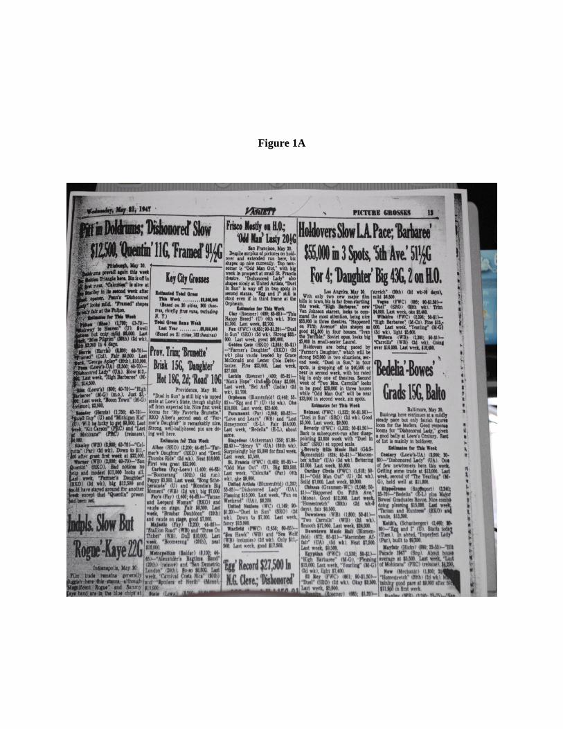
Figure 1A

 

 

 

 

Figure 1B

Publication Date City

 

 

Theater name (Theater’s Owner) (Seat Capacity; Price Range)

 

 

“Movie” (Distributor), $ Box Office Revenue

 

Figure 2

.51

1.5

22

.53

Mo

vie

Tic

ket P

rice

0 200 400 600Week 1945 - 1955

Radio City Music Hall Ticket Prices Between 1945 and 1955

Figure 3

Figure 4

Figure 5

020

40

60

80

TV

satu

ratio

n

1940 1945 1950 1955 1960Year

% US Homes with TV 1940-1959

Table 1. City and Year Structure of Data Set

City 1945 1946 1947 1948 1949 1950 1951 1952 1953 1954 1955 Theaters Total

Baltimore, MD 8 9 8 8 8 7 8 9 9 10 10 12Birmingham, AL 0 0 0 0 0 0 5 0 0 0 0 5Boston, MA 12 15 17 15 13 12 12 12 14 13 13 22Buffalo, NY 5 6 6 6 6 5 5 5 7 6 6 7Chicago, IL 11 11 13 14 15 14 12 12 16 16 16 21Cincinnati, OH 9 8 8 7 8 7 8 6 6 6 5 13Cleveland, OH 7 7 9 8 7 8 10 8 8 8 7 11Columbus, OH 4 0 0 0 0 0 0 0 0 0 0 4Denver, CO 9 9 11 10 14 11 11 12 12 11 14 23Detroit, MI 8 8 9 9 7 7 8 6 9 9 9 12Indianapolis, IN 5 5 5 5 5 5 5 5 5 5 5 5Kansas City, MO 7 7 11 9 11 10 12 14 13 13 12 18Lincoln, NE 0 5 0 0 0 0 0 0 0 0 0 5Los Angeles, CA 27 31 38 36 39 33 33 28 33 34 32 55Louisville, KY 7 7 8 8 8 4 5 5 4 4 4 8Minneapolis, MN 9 10 12 12 11 10 9 10 9 8 8 12New York, NY 18 21 26 25 21 21 24 26 27 28 24 42Omaha, NE 5 5 5 5 6 5 5 5 4 4 7 8Philadelphia, PA 11 11 13 13 14 13 12 13 13 12 13 17Pittsburgh, PA 8 7 8 7 7 8 6 6 6 6 7 12Portland, OR 8 8 9 9 9 6 7 9 9 8 6 11Providence, RI 8 7 7 7 7 7 6 5 5 5 4 8Saint Louis, MO 6 6 10 8 9 6 8 9 8 9 10 13San Francisco, CA 8 10 15 16 13 14 11 11 13 14 13 19Seattle, WA 11 10 11 11 10 9 9 10 9 9 8 12Washington, DC 6 8 10 11 11 11 9 10 10 10 11 18

Theaters/Year 217 231 269 259 259 233 240 236 249 248 244 393Cities/Year 24 24 23 23 23 23 24 23 23 23 23 26

Note: This table indicates the number of theaters per city and year for which the data set used in this paper

has information.

Table 2. Boston Panel Data Set with Vertical integration in Yellow

Theaters 1945 1946 1947 1948 1949 1950 1951 1952 1953 1954 1955 Total # Weeks

Astor - - 5 52 38 49 52 51 51 51 50 349Beacon Hill - - - 3 - 16 18 41 17 44 49 188Boston 51 50 50 52 51 46 52 52 45 51 26 526Cinerama - - - - - - - - - - 21 21Center - - 4 - - - - - - - - 4Esquire - 34 33 6 12 1 - - 4 - - 90Exeter - 1 27 50 15 - 16 49 51 51 47 307Fenway 51 50 50 51 50 52 52 53 51 45 49 554Kenmore - - 18 16 - - - - - - 28 62Majestic 43 37 25 5 11 - 19 1 6 8 - 155Mayflower - - - - 26 8 - - 3 - 12 49Memorial 51 48 48 52 50 52 52 53 51 51 49 11Modern - - 11 - - - - - - - - 557Metropolitan 50 50 49 51 51 51 52 53 51 51 50 559Normandi 1 - - - - - - - - - - 1Old South 8 12 11 3 - - - - - - - 34Olympia - 1 - - - - - - - - - 1Pilgrim - - - - 19 12 - 6 12 36 18 103Orpheum 51 49 50 52 51 49 52 52 51 51 47 555Paramount 50 49 50 52 51 52 52 53 51 50 45 555Scoltay - 1 - - - - - - - - - 1State 50 50 50 52 51 50 52 52 50 51 49 557Tremont 18 41 5 - - - - - - - - 64Translux 50 49 46 6 - - 1 - - 2 - 154

Note: Every cell contains the number of weeks for which information on givent theater was reported.Yellow color indicates vertically integrated theater, white color otherwise.Green color indicates different names to a same theater (according to Cinematreasures.com).

Table 3. San Francisco Panel Data Set with Vertical Integration in Yellow

Theaters 1945 1946 1947 1948 1949 1950 1951 1952 1953 1954 1955 Total # Weeks

Bridge - - - - - - - - 9 32 39 80Center - - 12 3 - - - - - - - 15Cinema - - - - - - - - 1 - - 1Clay - - 31 30 33 43 34 46 44 35 40 336Esquire - 2 17 43 32 6 - - 4 4 - 108Fox 45 45 50 49 47 50 48 53 48 49 50 534Geary - - - 2 - 5 - - - - - 7Golden Gate 46 45 48 49 47 50 48 53 48 49 49 532Guild - - 17 1 - - - - - - - 18Larkin - - 26 34 14 42 30 31 33 40 45 295Orpheum 38 44 49 49 47 50 48 53 40 49 50 517Paramount 46 44 50 49 47 50 48 53 48 49 50 534Rio - - - - - - - - - - 22 22St. Francis 46 40 38 49 47 50 48 53 48 48 50 517Stagedoor - 5 47 36 41 42 46 50 47 47 48 409State 45 44 23 45 10 2 - - - 5 - 174United Artists 38 43 50 49 47 50 48 53 48 49 50 525United Nations - - 39 46 10 4 - - - - - 99Vogue - - - - - - 32 29 39 42 44 186Warfield 45 45 50 49 46 50 48 52 48 48 49 530

Note: Every cell contains the number of weeks for which information on givent theater was reported.Yellow color indicates vertically integrated theater, white color otherwise.

Table 4. New York City Panel Data Structure with Vertical Integration in Yellow

Theaters 1945 1946 1947 1948 1949 1950 1951 1952 1953 1954 1955 Total # Weeks

Ambassador 13 1 5 25 1 7 ‐ ‐ ‐ ‐ ‐ 52

Astor 51 51 52 52 50 48 52 53 48 51 51 559

Baronet ‐ ‐ ‐ ‐ ‐ ‐ ‐ 13 49 49 42 153

Beekman ‐ ‐ ‐ ‐ ‐ ‐ ‐ 14 3 ‐ ‐ 17

Bijou ‐ ‐ 10 31 51 51 49 11 17 10 ‐ 230

Broadway ‐ ‐ 27 ‐ ‐ ‐ ‐ 12 21 6 ‐ 66

Capitol 52 51 52 52 51 52 52 52 51 51 51 567

Criterion 52 50 52 52 51 52 52 53 51 50 51 566

Elysee ‐ ‐ ‐ 8 ‐ ‐ ‐ ‐ ‐ ‐ ‐ 8

Embassy ‐ ‐ ‐ ‐ ‐ 2 ‐ ‐ ‐ 1 ‐ 3

Fine Arts ‐ ‐ ‐ ‐ ‐ ‐ 10 53 51 51 51 216

Fulton ‐ ‐ 6 2 2 ‐ ‐ ‐ ‐ ‐ ‐ 10

Globe 49 50 51 52 51 52 52 49 50 51 49 556

Golden ‐ 15 19 15 ‐ ‐ 7 ‐ ‐ ‐ ‐ 56

Gotham 52 51 52 14 20 ‐ ‐ ‐ ‐ ‐ ‐ 189

Guild ‐ ‐ ‐ ‐ ‐ ‐ ‐ 14 37 49 51 151

Holiday ‐ ‐ ‐ ‐ ‐ ‐ 18 14 48 32 ‐ 112

Hollywood 52 51 32 ‐ ‐ ‐ ‐ ‐ ‐ ‐ ‐ 135

Little Carnegie ‐ ‐ 16 18 ‐ ‐ ‐ ‐ ‐ 23 40 97

Mayfair ‐ 1 17 52 51 52 52 52 51 50 51 429

New York ‐ ‐ ‐ ‐ ‐ ‐ ‐ ‐ 4 5 ‐ 9

Normandie ‐ ‐ ‐ ‐ ‐ ‐ ‐ 47 39 48 49 183

Palace 52 51 52 51 49 52 40 34 43 48 49 521

Paramount 52 51 52 52 51 52 52 53 51 51 51 568

Paris ‐ ‐ ‐ ‐ ‐ ‐ 14 52 51 51 51 219

Park Avenue ‐ ‐ 48 32 50 37 39 44 ‐ ‐ ‐ 250

Plaza ‐ ‐ ‐ ‐ ‐ ‐ ‐ ‐ ‐ ‐ 17 17

Radio City Music Hall 52 51 51 52 51 52 52 52 50 51 51 565

Republic 16 15 ‐ ‐ ‐ ‐ ‐ ‐ ‐ ‐ ‐ 31

Rialto 52 51 52 52 51 48 8 15 11 ‐ ‐ 340

Rivoli 52 51 51 52 51 52 42 41 50 31 19 492

Roxy 52 51 52 52 51 51 52 50 48 51 50 560

State 52 51 52 52 51 51 52 53 51 51 50 566

Strand 52 51 52 52 49 52 22 ‐ ‐ ‐ ‐ 330

Sutton ‐ ‐ 16 17 36 52 52 53 48 47 51 372

Trans‐Lux 52nd Street ‐ ‐ ‐ ‐ ‐ 6 52 53 51 51 51 264

Trans‐Lux 60th Street ‐ ‐ ‐ ‐ 1 44 45 53 51 48 2 244

Uptown ‐ 1 ‐ ‐ ‐ ‐ ‐ ‐ ‐ ‐ ‐ 1

Victoria 52 51 52 35 50 52 52 52 51 51 51 549

Warner ‐ ‐ 19 20 ‐ ‐ 25 20 29 51 51 215

Winter Garden 11 51 52 38 ‐ ‐ ‐ ‐ ‐ ‐ ‐ 152

World ‐ ‐ ‐ ‐ ‐ ‐ ‐ ‐ ‐ ‐ 6 6

Note: Every cell contains the number of weeks for which information on givent theater was reported.Yellow color indicates vertically integrated theater, white color otherwise.

Table 5. Year of TV Introduction Across Cities in Sample

Year of TV Introduction Cities Cum Cities Cum Pop (as of 1950)

1945 ‐ 0 0

1946New York City, Chicago, Philadelphia, Los Angeles, 

Washington DC5 16357060

1947 Detroit, Saint Louis 7 19063424

1948 Baltimore, Cleveland, Boston, Buffalo, Minneapolis, Cincinnati 13 23335232

1949San Francisco, Pittsburgh, Seattle, Indianapolis, Louisville, 

Omaha, Providence, Columbus, Birmingham22 27579054

1950 Kansas City 23 28035676

1951 ‐ 23 28035676

1952 Denver 24 28451462

1953 Portland, Lincoln 26 28923974

1954 ‐ 26 28923974

1955 ‐ 26 28923974

Table 6. General Summary Statistics and by Organizational Form

Theater Ever Integ? DifferenceVariable Obs Mean Std. Dev. Min Max ==1 ==0 (==0) - (==1)

Evening Price 106702 1.00 0.40 0.25 3.6 0.999 0.991 -0.0070.002 0.002 0.003

Matinee Price 106702 0.59 0.23 0.09 2.4 0.579 0.613 0.0340.001 0.001 0.001

Theater Integ? 106702 0.34 0.48 0 1 0.568 0 -0.5680.002 0 0.002

Theater Ever Integ? 106702 0.61 0.49 0 1 - - -- - -

Box Office Revenues 106665 14232.33 15616.90 300 850000 16622.10 10559.57 -6062.5369.37 53.09 96.07

Tickets Sold 106665 14349.25 11981.30 300 894737 16304.99 11343.54 -4961.4547.69 54.18 73.52

Years Since TV Intro 106702 2.90 2.86 0 9 2.87 2.95 0.080.01 0.01 0.02

HHI 106702 989.70 1114.55 89.4438 10000 837.51 1223.55 386.03(by theater number) 3.05 7.13 6.88

No. Screens 393 1.03 0.23 1 3 1.03 1.04 0.010.02 0.02 0.02

Capacity per Screen 393 1575.08 1053.15 115 5945 2049.98 1209.28 -840.7083.47 57.81 98.51

Note: This table presents summary statistics of all variables used in this paper. See that variables that do not vary across time (number of screens and capacity per screen) have summary statistics at the theater level.The second part of the table provides summary statistics by whether the theater was EVER vertically integrated and the last column. calculates differences across the two groups of theaters.Numbers in smaller font size are standard errors for the averages at the group level and differences.

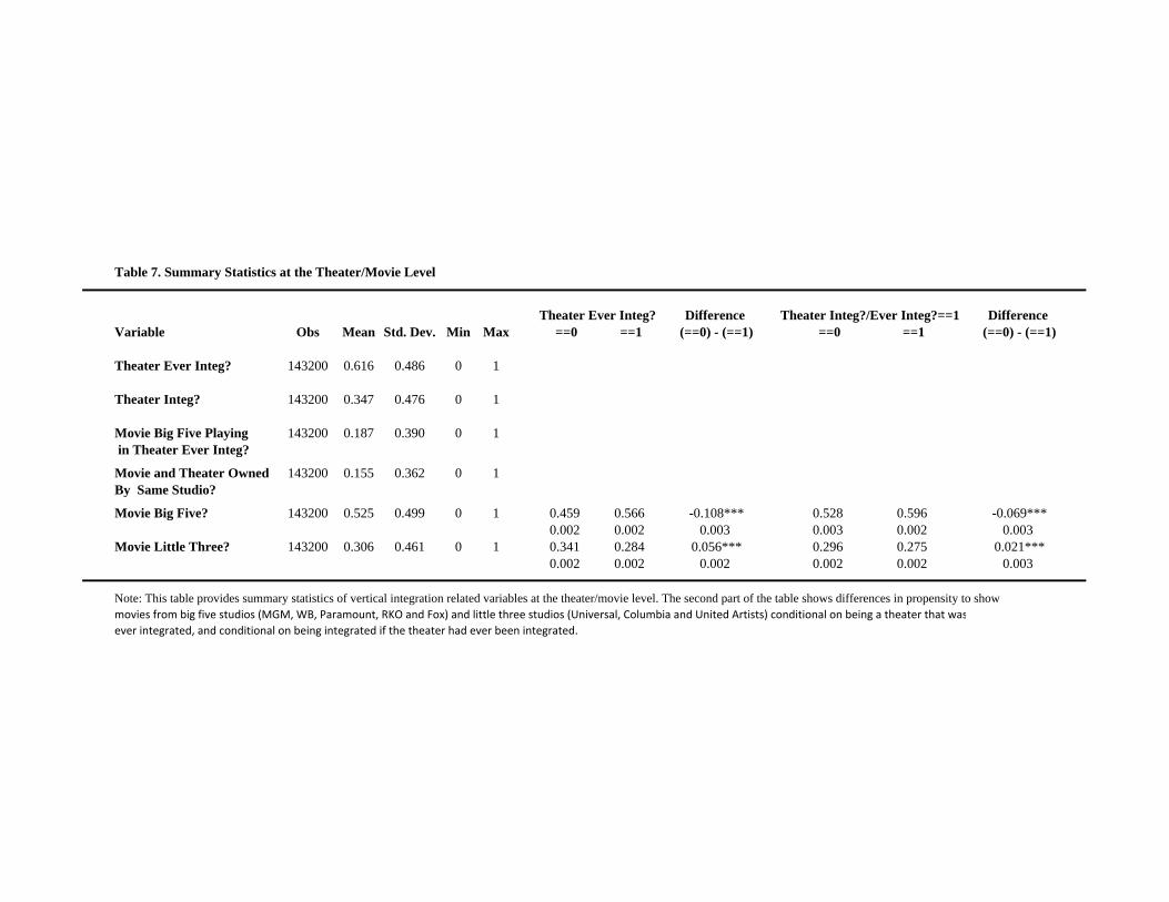
Table 7. Summary Statistics at the Theater/Movie Level

Theater Ever Integ? Difference Theater Integ?/Ever Integ?==1 DifferenceVariable Obs Mean Std. Dev. Min Max ==0 ==1 (==0) - (==1) ==0 ==1 (==0) - (==1)

Theater Ever Integ? 143200 0.616 0.486 0 1

Theater Integ? 143200 0.347 0.476 0 1

Movie Big Five Playing 143200 0.187 0.390 0 1 in Theater Ever Integ?

Movie and Theater Owned 143200 0.155 0.362 0 1By Same Studio?

Movie Big Five? 143200 0.525 0.499 0 1 0.459 0.566 -0.108*** 0.528 0.596 -0.069***0.002 0.002 0.003 0.003 0.002 0.003

Movie Little Three? 143200 0.306 0.461 0 1 0.341 0.284 0.056*** 0.296 0.275 0.021***0.002 0.002 0.002 0.002 0.002 0.003

Note: This table provides summary statistics of vertical integration related variables at the theater/movie level. The second part of the table shows differences in propensity to showmovies from big five studios (MGM, WB, Paramount, RKO and Fox) and little three studios (Universal, Columbia and United Artists) conditional on being a theater that was

ever integrated, and conditional on being integrated if the theater had ever been integrated.

Table 8. Vertical Integration and Evening Prices

(1) (2) (3) (4) (5) (6)

Dep Var Evening Price ln [Evening Price]

Theater Ever Integ? -0.010 0.009 0.009(0.038) (0.032) (0.031)

Theater Integ? 0.000 -0.042** -0.038** 0.006 0.133*** 0.140***(0.029) (0.018) (0.018) (0.015) (0.039) (0.041)

No Screens -0.027 -0.024 -0.021(0.032) (0.028) (0.028)

Capacity per Screen 0.00001 0.00001 0.00001(0.00001) (0.00001) (0.00001)

Years TV Intro 0.072*** 0.052*** 0.031*** 0.006 0.014*** 0.015***(0.005) (0.004) (0.007) (0.004) (0.004) (0.004)

HHI -0.00005*** -0.00001 -0.00001 -0.000002 -0.000001 -0.000001(0.00001) (0.00001) (0.00001) (0.00001) (0.00001) (0.00001)

Theater Ever Integ?*YearWeek 0.0007***(0.0001)

Theater Integ?*YearWeek -0.0004**(0.0001)

YearWeek 0.0004***(0.0001)

Theater Ever Integ?*YearMonth 0.0015***(0.0001)

Theater Integ?*YearMonth -0.0018***(0.0001)

YearMonth 0.0021***(0.0001)

Theater Ever Integ?*Year 0.0169***(0.006)

Theater Integ?*Year -0.0211*** (0.005)

Year 0.0243***(0.004)

Constant 0.849*** 0.864*** 0.827*** -0.251*** -0.317*** -0.330***(0.076) (0.051) (0.053) (0.012) (0.024) (0.025)

City FE No Yes Yes No No NoYear FE No No Yes Yes No NoTheater FE No No No Yes Yes Yes

Observations 106,702 106,702 106,702 106,702 106,702 106,702R-squared 0.26 0.51 0.53 0.77 0.77 0.77

Note: This table regress Evening Price and its natural logarithm on vertical integration variables.Robust standard errors in parentheses, clustered at the theater level. *** p<0.01, ** p<0.05, * p<0.1

Table 9 Vertical Integration and Matinee PricesTable 9. Vertical Integration and Matinee Prices

(1) (2) (3) (4) (5) (6)

Dep Var Matinee Price ln [Matinee Price]

Theater Ever Integ? -0.016 -0.041*** -0.043***(0.020) (0.015) (0.015)

Theater Integ? 0.001 -0.002 0.007 0.031* 0.181*** 0.192***(0.013) (0.010) (0.009) (0.017) (0.035) (0.037)

No Screens -0.051** -0.027 -0.025(0.021) (0.017) (0.016)

Capacity per Screen -0.00002** -0.00001*** -0.00001***(0.00001) (0.00001) (0.00001)

Years TV Intro 0.041*** 0.036*** 0.0002 -0.020*** 0.003 0.003(0.002) (0.002) (0.004) (0.005) (0.005) (0.005)

HHI 0.00001 0.00001* 0.000006* 0.00001** 0.00001 0.00001(0.00001) (0.00001) (0.00004) (0.000001) (0.00001) (0.00001)

Theater Ever Integ?*YearWeek 0.0006***(0.0001)

Theater Integ?*YearWeek -0.0006***(0.0001)

YearWeek 0.0007***(0.0001)

Theater Ever Integ?*YearMonth 0.001**(0.001)

Theater Integ?*YearMonth -0.003***(0.001)

YearMonth 0.004***(0.001)

Theater Ever Integ?*Year 0.014**(0.007)

Theater Integ?*Year -0.029***(0.005)

Year 0.047***(0.005)

Constant 0.567*** 0.561*** 0.528*** -0.847*** -0.941*** -0.964***(0.037) (0.027) (0.025) (0.016) (0.023) (0.025)

City FE No Yes Yes No No NoYear FE No No Yes Yes No NoTheater FE No No No Yes Yes Yes

Observations 106,702 106,702 106,702 106,702 106,702 106,702R d 0 28 0 51 0 54 0 78 0 76 0 76R-squared 0.28 0.51 0.54 0.78 0.76 0.76

Note: This table regress Matinee Price and its natural logarithm on vertical integration variables.Robust standard errors in parentheses, clustered at the theater level. *** p<0.01, ** p<0.05, * p<0.1

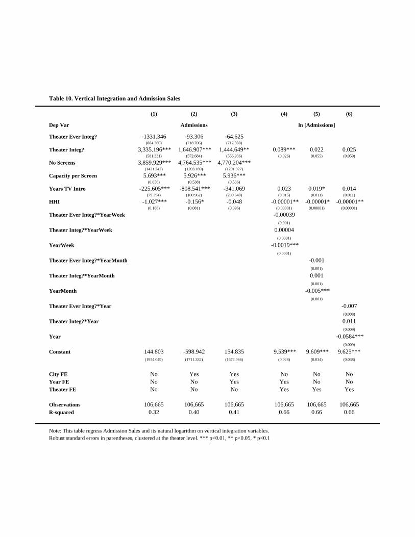
Table 10. Vertical Integration and Admission Sales

(1) (2) (3) (4) (5) (6)

Dep Var Admissions ln [Admissions]

Theater Ever Integ? -1331.346 -93.306 -64.625(884.360) (718.706) (717.988)

Theater Integ? 3,335.196*** 1,646.907*** 1,444.649** 0.089*** 0.022 0.025(581.331) (572.684) (566.936) (0.026) (0.055) (0.059)

No Screens 3,859.929*** 4,764.535*** 4,770.204***(1431.242) (1203.189) (1201.927)

Capacity per Screen 5.693*** 5.926*** 5.936***(0.656) (0.538) (0.536)

Years TV Intro -225.605*** -808.541*** -341.069 0.023 0.019* 0.014(79.394) (100.962) (280.640) (0.015) (0.011) (0.011)

HHI -1.027*** -0.156* -0.048 -0.00001** -0.00001* -0.00001**(0.188) (0.081) (0.096) (0.00001) (0.00001) (0.00001)

Theater Ever Integ?*YearWeek -0.00039(0.001)

Theater Integ?*YearWeek 0.00004(0.0001)

YearWeek -0.0019***(0.0001)

Theater Ever Integ?*YearMonth -0.001(0.001)

Theater Integ?*YearMonth 0.001(0.001)

YearMonth -0.005***(0.001)

Theater Ever Integ?*Year -0.007(0.008)

Theater Integ?*Year 0.011(0.009)

Year -0.0584***(0.009)

Constant 144.803 -598.942 154.835 9.539*** 9.609*** 9.625***(1954.049) (1711.332) (1672.066) (0.028) (0.034) (0.038)

City FE No Yes Yes No No NoYear FE No No Yes Yes No NoTheater FE No No No Yes Yes Yes

Observations 106,665 106,665 106,665 106,665 106,665 106,665R-squared 0.32 0.40 0.41 0.66 0.66 0.66

Note: This table regress Admission Sales and its natural logarithm on vertical integration variables.Robust standard errors in parentheses, clustered at the theater level. *** p<0.01, ** p<0.05, * p<0.1

Table 11. Vertical Integration and Box Office RevenuesTable 11. Vertical Integration and Box Office Revenues

(1) (2) (3) (4) (5) (6)

Dep Var Box Office Revenues ln [Box Office Revenues]

Theater Ever Integ? -1263.64 424.11 450.08(1220.86) (1008.56) (1006.50)

Theater Integ? 2,921.71*** 565.24 455.85 0.094*** 0.155*** 0.165***(848.05) (779.37) (785.64) (0.03) (0.06) (0.06)

N S 4 676 69** 6 197 46*** 6 231 92***No Screens 4,676.69** 6,197.46*** 6,231.92***(1825.51) (1846.27) (1856.40)

Capacity per Screen 7.16*** 7.62*** 7.63***(1.79) (1.50) (1.50)

Years TV Intro 780.06*** -163.66 -22.81 0.029* 0.032*** 0.029***(155.98) (106.17) (257.27) (0.02) (0.01) (0.01)

HHI -1.87*** -0.17* -0.19* -0.00002** -0.00001* -0.00001**(0.46) (0.09) (0.11) (0.00001) (0.00001) (0.00001)

Theater Ever Integ?*YearWeek 0.000256(0 001)(0.001)

Theater Integ?*YearWeek -0.00037(0.001)

YearWeek -0.0015***(0.0001)

Theater Ever Integ?*YearMonth 0.000811(0.001)

Theater Integ?*YearMonth -0.000797(0 001)(0.001)

YearMonth -0.0031***(0.001)

Theater Ever Integ?*Year 0.010(0.008)

Theater Integ?*Year -0.010(0.009)

Year -0.034***(0 009)(0.009)

Constant -5769.790072 -7415.93* -7590.68* 9.289*** 9.292*** 9.294***(4,352.24) (4,028.56) (4,136.70) (0.029) (0.035) (0.039)

City FE No Yes Yes No No NoYear FE No No Yes Yes No NoTheater FE No No No Yes Yes Yes

Observations 106,665 106,665 106,665 106,665 106,665 106,665R d 0 28 0 46 0 46 0 68 0 68 0 68R-squared 0.28 0.46 0.46 0.68 0.68 0.68

Note: This table regress Box Office Revenues and its natural logarithm on vertical integration variables.Robust standard errors in parentheses, clustered at the theater level. *** p<0.01, ** p<0.05, * p<0.1

Table 12. Vertical Integration, Admissions Sales and Box Office Revenues After Dropping Observations with Joint Reporting

(1) (2) (3) (4) (5) (6) (7) (8) (9) (10) (11) (12)( ) ( ) ( ) ( ) ( ) ( ) ( ) ( ) ( ) ( ) ( ) ( )

Dep Var Admissions ln [Admissions] Box Office Revenues ln [Box Office Revenues]

Theater Ever Integ? -1971.41** -506.14 -450.59 -1781.08 22.96 93.36(940.71) (754.21) (754.80) (1312.28) (1067.99) (1062.58)

Theater Integ? 2,644.71*** 1,071.56* 829.66 0.07*** 0.06 0.07 2,271.69** -126.80 -326.74 0.08*** 0.20*** 0.22***(631.96) (609.81) (614.62) (0.03) (0.05) (0.05) (948.33) (904.00) (924.81) (0.03) (0.05) (0.06)

No Screens 3,827.73** 4,581.07*** 4,604.37*** 4,540.80** 6,113.88*** 6,161.17***(1550 70) (1289 33) (1290 71) (1800 83) (1937 74) (1950 11)(1550.70) (1289.33) (1290.71) (1800.83) (1937.74) (1950.11)

Capacity per Screen 6.08*** 6.16*** 6.18*** 7.50*** 7.89*** 7.93***(0.68) (0.55) (0.54) (1.86) (1.57) (1.58)

Years TV Intro -331.66*** -1030.59*** -957.99*** -0.019 -0.008 -0.013 692.48*** -369.06*** -575.56** -0.011 0.008 0.004(82.10) (107.75) (274.73) (0.012) (0.009) (0.009) (177.57) (113.79) (263.98) (0.012) (0.008) (0.009)

HHI -1.02*** -0.13 -0.03 -0.00001** -0.00001** -0.00001** -1.88*** -0.15 -0.17 -0.00002** -0.00001** -0.00001**(0.20) (0.08) (0.10) (0.00001) (0.00001) (0.00001) (0.49) (0.10) (0.12) (0.00001) (0.00001) (0.00001)

Theater Ever Integ?*YearWeek -0.0003 0.0003(0 001) (0 001)(0.001) (0.001)

Theater Integ?*YearWeek -0.0002 -0.0006*(0.001) (0.000)

YearWeek -0.0018*** -0.0014***(0.001) (0.001)

Theater Ever Integ?*YearMonth -0.0011* 0.000451(0.001) (0.001)

Theater Integ?*YearMonth -0.0005 -0.0022***(0 001) (0 001)(0.001) (0.001)

YearMonth -0.0037*** -0.0017***(0.001) (0.001)

Theater Ever Integ?*Year -0.012 0.0059(0.008) (0.009)

Theater Integ?*Year -0.007 -0.0268***(0.007) (0.008)

Year -0.0397*** -0.0166**(0 008) (0 008)(0.008) (0.008)

Constant -199.304 -494.853 314.51 9.561*** 9.582*** 9.587*** -5938.884 -7537.355* -7638.24* 9.299*** 9.256*** 9.249***(2066.942) (1778.108) (1,743.06) (0.024) (0.030) (0.033) (4516.646) (4240.929) (4,337.21) (0.026) (0.033) (0.037)

City FE No Yes Yes No No No No Yes Yes No No NoYear FE No No Yes Yes No No No No Yes Yes No NoTheater FE No No No Yes Yes Yes No No No Yes Yes Yes

Observations 97,089 97,089 97,089 97,089 97,089 97,089 97,089 97,089 97,089 97,089 97,089 97,089R-squared 0.36 0.45 0.46 0.71 0.71 0.71 0.30 0.49 0.49 0.73 0.72 0.72R squared 0.36 0.45 0.46 0.71 0.71 0.71 0.30 0.49 0.49 0.73 0.72 0.72

Note: This table regresses Admissions Sales and Box Office Revenues (and their) natural logarithm on vertical integration variables. I drop observations from cities and years with joint reporting.Robust standard errors in parentheses, clustered at the theater level. *** p<0.01, ** p<0.05, * p<0.1

Table 13. Cross-Sectional Analysis at the Theater-Movie LevelTable 13. Cross-Sectional Analysis at the Theater-Movie Level

(1) (2) (3) (4) (5) (6) (7) (8) (9) (10) (11) (12)

Dep Var Evening Price Matinee Price Admissions per Movie Box Office per Movie

Theater Ever Integ? -0.004 0.016 0.013 -0.010 -0.028* -0.033** -1244.92* -420.65 -357.16 -1102.33 78.17 111.97(0.034) (0.028) (0.027) (0.020) (0.014) (0.014) (733.39) (654.24) (652.48) (999.14) (884.48) (883.13)

Theater Integ? 0.009 -0.030* -0.024 -0.001 -0.007 0.004 3251.46*** 1534.30*** 1288.27** 3279.94*** 1051.58* 919.21(0.025) (0.016) (0.015) (0.013) (0.010) (0.009) (538.99) (532.61) (518.96) (731.49) (597.17) (591.17)

Theater Integ, Studio Movie? -0.003 0.006 -0.001 0.022 0.017 0.007 378.79 1150.82 1190.13 -4.02 799.05 807.53(0.042) (0.025) (0.024) (0.017) (0.011) (0.011) (979.70) (841.84) (829.65) (1297.01) (797.40) (787.76)

Theater Ever Integ, Studio Movie? 0.010 -0.021 -0.016 -0.014 -0.012 -0.005 15.25 -1223.49 -1205.86 -76.49 -1765.03 -1734.82(0.048) (0.028) (0.027) (0.015) (0.010) (0.010) (894.49) (812.54) (793.51) (2084.97) (1769.42) (1767.76)

Movie Big Five? -0.049** -0.045** -0.042** -0.027*** -0.018** -0.017** 1240.27*** 1203.09*** 1133.50*** 1401.99** 1328.69** 1303.30**(0.023) (0.021) (0.020) (0.010) (0.008) (0.008) (340.87) (259.21) (251.84) (680.66) (526.87) (527.31)

Movie Little Three? -0.036 -0.038* -0.037* -0.019** -0.015* -0.016* 295.39 114.95 90.13 8.10 -236.95 -242.38Movie Little Three? 0.036 0.038 0.037 0.019 0.015 0.016 295.39 114.95 90.13 8.10 236.95 242.38(0.022) (0.021) (0.020) (0.010) (0.009) (0.009) (223.86) (204.36) (203.43) (311.53) (278.17) (276.26)

No Screens -0.030 -0.016 -0.012 -0.055*** -0.021* -0.019 3414.67*** 4182.90*** 4188.53*** 3918.89*** 5355.54*** 5391.84***(0.028) (0.021) (0.022) (0.018) (0.013) (0.013) (1236.73) (1097.61) (1090.90) (1471.87) (1535.73) (1541.09)

Capacity per Screen 0.00000 0.00001 0.00001 -0.00001* -0.00001** -0.00001** 4.81*** 5.18*** 5.19*** 5.73*** 6.45*** 6.46***(0.00001) (0.00001) (0.00001) (0.00001) (0.00001) (0.00001) (0.59) (0.52) (0.52) (1.51) (1.35) (1.35)

Years TV Intro 0.068*** 0.047*** 0.025*** 0.040*** 0.035*** -0.002 -113.69 -705.71*** -131.26 760.09*** -142.77 117.35(0.004) (0.003) (0.005) (0.002) (0.002) (0.003) (83.91) (94.56) (252.63) (150.29) (95.97) (229.32)

HHI 0 00004*** 0 00001 0 00001 0 000004 0 000005* 0 00001* 0 93*** 0 18** 0 08 1 61*** 0 18** 0 17**HHI -0.00004*** -0.00001 -0.00001 0.000004 0.000005* 0.00001* -0.93*** -0.18** -0.08 -1.61*** -0.18** -0.17**(0.00001) (0.00001) (0.00001) (0.00001) (0.000001) (0.000001) (0.17) (0.07) (0.09) (0.40) (0.08) (0.09)

Constant 0.88*** 0.87*** 0.83*** 0.57*** 0.55*** 0.52*** 95.43 -325.33 632.08 -4654.75 -6239.21 -6221.45(0.07) (0.05) (0.05) (0.03) (0.02) (0.02) (1804.47) (1669.85) (1634.07) (3936.92) (3817.49) (3910.98)

City FE No Yes Yes No Yes Yes No Yes Yes No Yes YesYear FE No No Yes No No Yes No No Yes No No Yes

Observations 143,200 143,200 143,200 143,200 143,200 143,200 143,153 143,153 143,153 143,153 143,153 143,153Observations 143,200 143,200 143,200 143,200 143,200 143,200 143,153 143,153 143,153 143,153 143,153 143,153R-squared 0.27 0.53 0.54 0.29 0.53 0.56 0.27 0.35 0.36 0.24 0.41 0.41

Note: This table shows cross-sectional OLS regressions for all four outcome variables using data at the theater-movie level. There are four new variables in this table that have not appeared before in the empirical analysis:i) "Theater Integ, Studio Movie?" equals 1 if integrated theater at a given point in time shows a movie of that same studio, and 0 otherwise.ii) "Theater Ever Integ, Studio Movie?" equals 1 if integrated theater ever shows a movie of the same studio that at some point owned that theater, and 0 otherwise.iii) "Movie Big Five?" equals 1 if movie was produced by one of the big five studios, RKO, Paramount, Fox, MGM or Warner Brothers, and 0 otherwise.iv) "Movie Little Three?" equals 1 if movie was produced by Columbia, Universal or United Artists, and 0 otherwise.Robust standard errors in parentheses, clustered at the theater level. *** p<0.01, ** p<0.05, * p<0.1.

Table 14. Demand Estimation for Movies

(1) (2) (3) (4) (5) (6) (7) (8) (9) (10) (11) (12)

OLS OLS OLS OLS OLS OLS OLS OLS OLS 2SLS 2SLS 2SLS

Evening Price -1.298*** -0.469*** -0.453*** -0.447*** -0.455*** -0.530*** -0.513*** -0.580 -0.798* -1.455*** -0.593*** -0.374***(0.106) (0.050) (0.05) (0.05) (0.05) (0.067) (0.041) (0.690) (0.496) (0.164) (0.069) (0.056)

No. Screens 0.311** 0.295** 0.246** 0.289 0.308*** 0.293**(0.099) (0.121) (0.111) (0.313) (0.097) (0.120)

Capacity per Screen 0.0004*** 0.0004*** 0.0003*** 0.0003 0.0004*** 0.0004***(0.0001) (0.0001) (0.0001) (0.0010) (0.0001) (0.0001)

Y TV I t 0 087*** 0 044*** 0 045*** 0 051*** 0 039** 0 052*** 0 076*** 0 047*** 0 050***Years TV Intro -0.087*** -0.044*** 0.045*** 0.051*** 0.039** 0.052*** -0.076*** 0.047*** 0.050***(0.009) (0.005) (0.017) (0.016) (0.015) (0.015) (0.012) (0.016) (0.015)

HHI 0.00004** -0.00003*** -0.00003*** -0.00002*** -0.00002 -0.00002*** 0.00003* -0.00003*** -0.00002***(0.00002) (0.00001) (0.00001) (0.00001) (0.00001) (0.00001) (0.00001) (0.00001) (0.00001)

Constant -4.208*** -3.939*** -5.363*** -3.858*** -4.716*** -4.364*** -3.248*** -4.915*** -4.104*** -4.079*** -4.918*** -3.596***(0.189) (0.044) (0.178) (0.055) (0.051) (0.186) (0.065) (0.822) (0.514) (0.218) (0.180) (0.054)

Theater FE No Yes No Yes Yes No Yes No Yes No No YesTheater FE No Yes No Yes Yes No Yes No Yes No No YesCity FE No No Yes No No Yes No No No No Yes NoYear/Week FE No No Yes Yes No Yes Yes No No No Yes YesCity/Year/Week FE No No No No Yes No No No No No No NoMovie FE No No No No No Yes Yes No No No No NoMovie/City/Year/Week FE No No No No No No No Yes Yes No No No

Observations 138,465 138,465 138,465 138,465 138,465 138,465 138,465 138,465 138,465 138,465 138,465 138,465, , , , , , , , , , , ,R-squared 0.49 0.82 0.75 0.83 0.86 0.796 0.854 0.98 0.99 0.49 0.75 0.83

Note: The dependent variable is natural logarithm of market share of a movie in a given city and week, that is, admission sales divided by city population.The last three columns show 2SLS regressions where I use Matinee Price as an instrument for Evening Price.Robust standard errors in parentheses, clustered at the theater level. *** p<0.01, ** p<0.05, * p<0.1.