1

Bundling and Complementarity

Thierno Diallo1

January 2005

Abstract

We analyze bundling incentives in markets where products are composed of two complementary components (e.g. hardware and software). One of the components is monopolized and the other is sold by a duopoly. We assume quality differentiation between components, and we develop a model of quality competition à la Mussa and Rosen (1978). We demonstrate that the monopolist’s bundling decision depends on the quality of the component where he faces competition. We show that: (i) if the monopolist’s component has a higher quality than the competitor’s, then the monopolist prefers not to bundle (separate selling); and (ii) if the quality of monopolist’s component is lower than the competitor’s, then the monopolist prefers bundling. Thus, the monopolist’s incentive not to bundle is related to narrowing of market for its monopolized component with bundling. We also consider a dynamic game where firms compete in two-stages (quality and price) and determine the subgame perfect Nash equilibrium. Finally, we discuss antitrust implications of these findings. Keywords: bundling, complementarity, quality, social welfare, antitrust. JEL Classification: L14, L15, L40, L41, L42

1I am indebted to Abraham Hollander and Lars Ehlers for continued guidance and encouragements. All errors are of course my own. Correspondence : Thierno Diallo, département de sciences économiques, Université de Montréal, C.P. 6128, succursale Centre-ville, Montréal QC H3C 3J7, Canada, email : thierno.diallo@umontreal.ca

2

I. Introduction I.1 Overview

Many products are consumed in combination with other products to form a complete

system of products that cannot be consumed separately. E.g., a computer system can be

decomposed into a basic unit and a monitor, a stereo system is an amplifier and a speaker,

a computer is composed of hardware and software. But products can be sold and

purchased either separately or as packages. Selling as packages can be achieved either by

technical bundling, i.e. by making one component compatible only with components sold

by the same firm or by engaging in tied selling.

A component is incompatible with components sold by other firms’, if it cannot be

assembled with them to form a usable system. The economic consequence of

compatibility versus incompatibility have been examined by Chou and Shy (1989),

Matutes and Regibeau (1989) for the case where each component is sold by an

independent firm. Matutes and Regibeau (1988), Economides (1989, 1991), and Einhorn

(1992) have looked at the case where each firm supplied all the components necessary to

form the complete system. Economides (1991) proved that for firms supplying all

components necessary to form a usable system, compatibility is profitable if the relative

increase in the demand for the systems when making components compatible exceeds the

number of complementary components supplied by other firms2. A standard result of this

literature is that compatibility increases industry demand and profits.

Tied selling or tying restrictions are of two types: requirement tie-ins and bundling.

Under requirement tie-ins the seller of product A requires all purchasers of A also to

purchase all their requirements of product B from him. Under a bundling arrangement or

package tie-ins the seller offers two or more products in fixed combination as a single

2 Formally, Economides (1991) considers a model where the market for one component (say market A ) is a duopoly, and the other (say market B ) is monopolistically competitive. He shows that when the addition of a new variety of B leads to little or no increase in the demand for the system AB , the profits of a firm of type- A are higher under incompatibility and they will choose this regime. By contrast, when the addition of a new variety of B increases the demand for the system AB , the profits of a firm of type- A are higher under compatibility. The profitability of compatibility depends on its capacity to increase the demand for A .

3

package. The difference between these two types of tying is that, in the case of bundling

the price of B is not separately stated but is bundled into the price of A .

A producer who makes its components incompatible with components produced by

others or engages in technical bundling imposes a de facto3 tie. In this paper, we are

interested in bundling. To rule out technical bundling, we assume a compatible world.

Thus, selling as packages is achieved only by bundling. We analyze bundling incentives

in markets where products are composed of two complementary components (e.g.

hardware and software) in the context of vertical product differentiation. One of the

components is monopolized and the other is sold by a duopoly. We ask what is the

monopolist’s best selling strategy between separate selling and bundling? What are the

consequences for welfare? To answer these questions, we review first the literature on

bundling and then we solve a model of quality competition for systems composed of two

complementary components.

I.2 The Bundling Literature

Three reasons are given in the literature to explain bundling. The traditional explanation

for bundling is that it achieves better price discrimination by a monopolist [Stigler

(1968), Adams and Yellen (1976), Schmalensee (1984), and McAfee, McMillan and

Whinston (1989)]. Usually, a firm has to charge one price to all consumers. In these cases

heterogeneity in consumers’ valuations frustrates the seller’s ability to capture consumer

surplus. Bundling reduces consumers’ heterogeneities in reservation prices and captures

the maximum of their surplus. Stigler’s analysis and Adams and Yellen (1976) are based

on stylized examples with a discrete number of customers. In these examples, the

reservation values of the components of the bundle are negatively correlated. Bundling

serves much the same purpose as price discrimination. Schmalensee (1984) considers the

entire class of Gaussian demands and shows that bundling also helps to reduce the

effective dispersion of reservation values and thereby makes it possible for the seller to

3 See Tirole (1988)

4

extract a greater fraction of the potential surplus even if demands are uncorrelated and

possibly positively correlated.

The second reason for bundling is the leveraging of market power that exists in one

market into another market, i.e. the use of monopoly power position in one market to

exclude rivals, deter entry or foreclose competition in others markets [Burstein (1960),

Blair (1978), Schmalensee (1982)]. As noted by Burstein (1960), firms can raise profits

by bundling goods that are complementary. Burstein has argued that a firm with a

monopoly over one good could monopolize another by selling them in conjunction with

each other. If it did so, a firm seeking to compete in the market for the bundled good

would be foreclosed from selling to all those who received the bundled good in

conjunction with their purchase of the bundling good. This theory has come under heavy

attack from the Chicago School [Director and Levi (1956), Posner (1976), Bork (1978)].

They argued that if a monopolist does employ tying or bundling, his motivation cannot be

leverage. The reason is that there is only one monopoly profit that can be extracted. Also,

they defended the fact that bundling could provide convenience for customer and lower

transaction cost. Whinston (1990) and Nalebuff (2004) re-examined the role of bundling

as an entry deterrent. Whinston (1990) presents a series of models in which he first makes

the assumption in which bundling does not increase profits and then alters the assumption

slightly so that it does. He shows that the Chicago School's criticism of leveraging

monopoly power from one market (say market A ) to another (say market B ) applies only

if market B is perfectly competitive. With this latter assumption he proves that the use of

leverage to affect the market B is actually impossible. However, when the monopolized

product A is no longer essential for all uses of product B , he shows that in the presence

of scale economies, bundling can be an effective and profitable strategy to alter market

structure by making continued operation unprofitable for bundled good rivals and

eventually induce them to exit. Due to the scale economies, an entrant would need to

attain sufficiently scale to survive in the market of B . Bundling can foreclose the entrant

from sales to be the difference between making entry profitable an unprofitable. In these

cases, bundling can increase the profits of the monopolist of A and harm consumers.

5

The third reason is that bundling leads to reduce costs by enabling economies of scope in

production and distribution to be achieved. Salinger (1995) recognizes that cost synergies

from bundling are most valuable when consumer valuations are positively correlated.

Focusing on the case of pure bundling, Salinger introduces the role of cost savings to

interact with demand effects and proposes a graphical analysis of the economic properties

of bundling. Thus, if most consumers would buy both (or neither) A and B when sold

separately, then any cost savings from selling them together will create an incentive for a

monopolist to sell bundled products when valuations are positively correlated.

Finally, we conclude this review of literature with the specific cases of complementary

and systems goods [Whinston (1990), Matutes and Regibeau (1992) and Economides

(1993)]. Here, price discrimination plays a minor role because the goods are highly

positively correlated in value and now there is more than one seller in the market

(oligopoly markets). For these specific cases, a standard result is that bundling is

dominated by separate selling. There is also no clear cut about welfare implications of

bundling in these studies. Whinston (1990) demonstrates that separate selling is more

profitable than pure bundling for a firm which is monopolist in A and faces a competitor

in B when consumers’ demands are for the system made by A and B . He shows that if a

commitment to bundling causes the competitor in B of the monopolist of A to be

inactive, the latter can do no worse and possibly better by committing to separate selling

(Proposition 3). This is because if the competitor is inactive, this reduces the sales of A .

Matutes and Regibeau (1992) and Economides (1993) extend the basic framework of

monopoly bundling to a duopoly setting, with horizontally differentiated components.

Here competition is between fully integrated firms, where each firm produces all

components necessary to form a system. Matutes and Regibeau (1992), show that if two

firms sell compatible components, then bundling is dominated by separate selling. This

result comes from two effects. For example, if we consider that two components ( A

and B ) are available, the first effect is that under compatibility separate selling increases

the number of systems that can be assembled from two ( AA and BB ) to four

( AA , AB , BA , BB ). This enables some consumers to obtain a system that is closer to

their ideal specification, and then industry demand is larger without bundling. The second

6

effect relates to the fact that separate selling softens price competition. The intuition is

that in a compatible world with separate selling a decrease in the price of one firm’s

component increases the demand for its own system, as well as for the mixed system

(system composed by different firms' components). However, the greater demand for the

mixed system reduces the demand for the firm’s second component. While with

bundling, if a firm lowers the price of one component, it attracts additional consumers for

its two components; cutting the price of one component increases equally the demand for

both components in the system. It follows that a firms’ price-cutting incentives are lower

with separate selling than with bundling.

I.3 Approach in this paper

This paper extends the literature on bundling in a number of ways. First, it considers

quality differences in system components with consumers’ taste à la Mussa and Rosen

(1978). Specifically, we study a market for systems composed of two complementary

components where we assume the unit cost increasing in quality and variable in

production4. One of the components is sold by a firm that has a monopoly in that

component; the other is sold by the same firm as well as by one other firm. Consumers

derive utility only from using one unit of the monopolized component in combination

with one unit of the other component.

Second, it answers the question how the introduction of quality affects the bundling

decision of a firm that is a monopolist for product A and faces a single competitor in

market for product B . We prove that the monopolist’s bundling decision depends on the

quality level of the component produced by two firms. We demonstrate that the

monopolist of A earns higher profits by selling A and B separately than selling the

system AB as bundle when its product B is of higher quality than that of its rival. On the

4 Quality differences in system components and consumers taste has been considered also by Einhorn (1992) and Economides and Lehr (1994). The former uses the model of quality differentiation of Gabszewicz and Thisse (1979) to analyze compatibility of systems’ components and find that profits are higher when components are fully compatible. The latter use the framework of Mussa and Rosen (1978) to study the quality choice of complete systems under many types of market structures with quadratic fixed cost of quality improvement. They do not find any equilibrium in quality in a similar market situation. In this paper by contrast, the unit cost is increasing in quality and variable in production. We find results that are qualitatively different and more general. As noted by Crampes and Hollander (1995), this specification of variable cost increasing in quality appears as the empirically more relevant case.

7

other hand if the monopolist’s product B has the lower quality, then the bundling

strategy yields more profits than separated selling. The intuitions for these results are

quite simple and similar to those of Economides (1991). The profitability of separate

selling depends on the relative increase in the demand for A compared to the losses

incurred due to competition faced in B . Separate selling leads to a considerable increase

in the demand for A through sales with B when the monopolist produces the higher

quality of B . Conversely, separate selling brings no increase in the demand for A when

the monopolist produces the lower quality of B . These results extend Whinston (1990)

and Matutes and Regibeau (1992), when firms’ components are vertically differentiated.

Also, in contrast to these studies, we demonstrate that bundling reduces social welfare.

Third, it considers the question how the decision to sell components separately or to

bundle affects quality choice. We model a two stages game. In the first stage, firms

choose qualities and determine whether they sell separately or bundle. In the second stage

they set prices. We find the set of equilibrium quality and pricing decisions for each firm

that are outcomes of the subgame perfect Nash equilibria. We show that a firm who is

monopolist in product A produces always the highest quality of product B and makes

more profits by selling A and B separately.

The plan of the paper is as follows. In section II, we present the model. In section III, we

determine the possible relevant selling strategies. In section IV, we study and compare

the separated selling strategy to the bundling strategy under different assumptions about

qualities of firms’ products. Also in this section, we perform a welfare analysis and we

investigate the endogenous case of quality choices with a quadratic cost function. Finally,

we give antirust implications of findings and conclude in section V.

II. The Model

There are two firms, denoted 1 and 2 and two products denoted A and B . Firm 1 sells the

products A and B , whereas firm 2 sells only product B . The product B comes in two

distinct levels of quality, high (H) and low (L). Quality means reliability. It is the

8

probability of not breaking down. Let Aα denote the probability that product A does not

breakdown. Similarly, let iBα denote the probability that product B of quality i not

breakdown, where { }LHi ,∈ . By assumptionLH BB αα > .

We simplify by assuming that A is produced at zero marginal cost with no fixed cost.

While B is produced at constant unit cost that depends on the probability of breakdown.

We assume the cost function to be of the form:

)(),( αα qcqC = ,

where q and α denote respectively the quantity of output and the probability that a

component does not breakdown5. Also, we assume that 0)(,0)(,0)( ≥′′≥′≥ ααα ccc for

allα . Convexity of the unit cost function implies forLH BB αα > , that:

0)()( >−LHHL BBBB cc αααα . (1)

Consumers derive utility only from using one unit of A in combination with one unit

of B . They can, however, combine A with any quality of B. Consumers are indexed byθ ,

where θ is uniformly distributed on ]1,0[ . When none of the component breakdown,

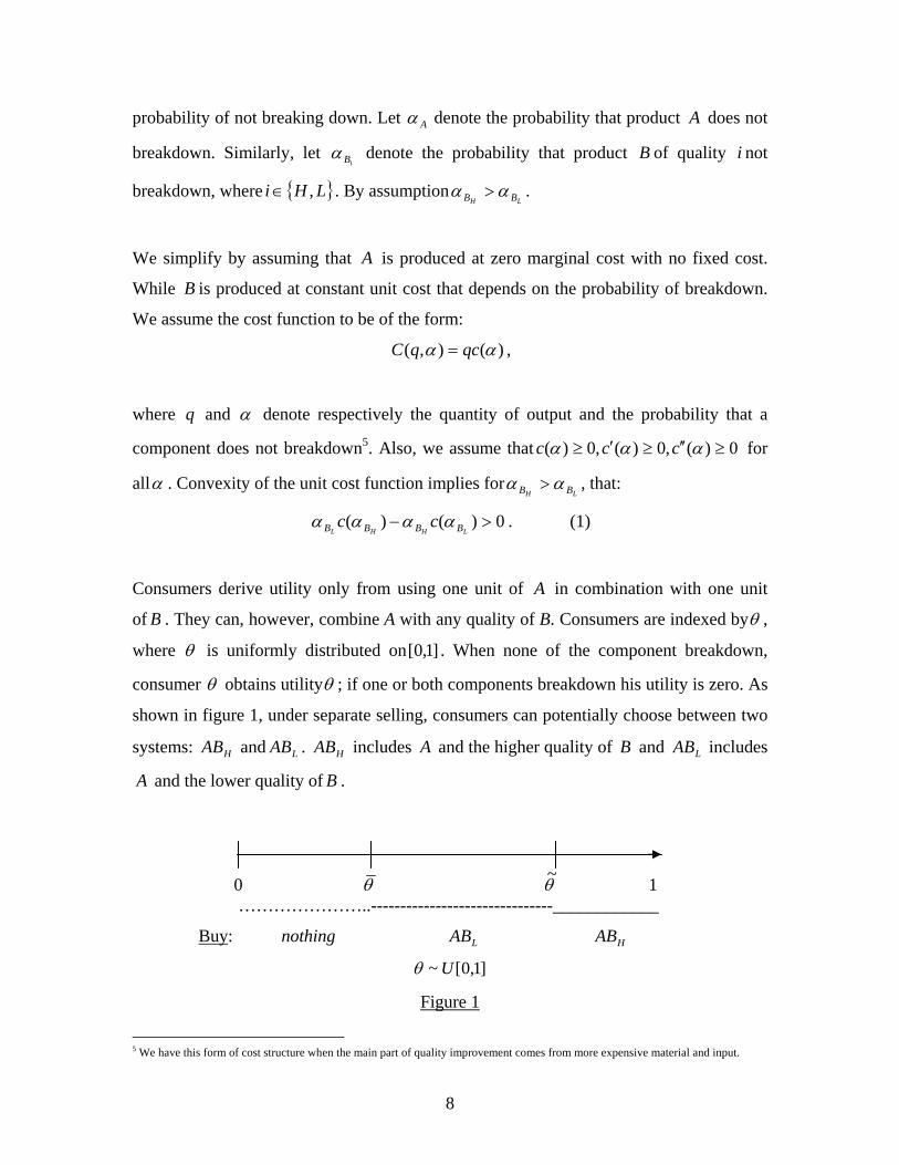
consumer θ obtains utilityθ ; if one or both components breakdown his utility is zero. As

shown in figure 1, under separate selling, consumers can potentially choose between two

systems: HAB and LAB . HAB includes A and the higher quality of B and LAB includes

A and the lower quality of B .

0 θ θ~ 1 …………………..-------------------------------____________

Buy: nothing LAB HAB

]1,0[~ Uθ

Figure 1

5 We have this form of cost structure when the main part of quality improvement comes from more expensive material and input.

9

We note byiABP , the price of the complete system iAB , { }LHi ,∈ . If the components of

the complete system are purchased individually, then the price of the complete system is

the sum of the individual components’ price )(iBA PP + . Else the price of the complete

system is the bundle priceiGP , where iG represents the bundle iAB , { }LHi ,∈ .

Consumers are assumed to be risk neutral. They maximize expected surplus. This means

that they choose the combination of reliabilities of A and B that maximizes:

ii ABBA P−θαα ,

{ }LHi ,∈ ,

where θααiBA , is the expected utility derived by consumers indexed θ from the quality i

of product B consumed with product A . We assume that the reliability of A

and iB , { }LHi ,∈ is common knowledge.

We indicate by θ~ the preference parameter of a consumer who is indifferent between

purchasing the higher quality system ( HAB ) and the lower quality system ( LAB ). The

consumer indexed θ is indifferent between purchasing the lower quality system ( LAB )

and not purchasing at all.

The demand function for each complete system depends on prices and breakdown

probabilities. To obtain the demands, we use the individual-rationality )(IR constraints

and the incentive constraints )(IC of each demand consumer. For the consumer who

purchases the higher quality system the following constraints are used:

0≥−HH ABBA Pθαα , )( HIR

LLHH ABBAABBA PP −≥− θααθαα . )(IC

10

For the one who purchases the lower quality system the individual rationality constraint

is:

0≥−LL ABBA Pθαα . )( LIR

This implies that)(

~

LH

LH

BBA

ABAB PPααα

θ−

−= . From the )( LIR constraint we derive:

L

L

BA

ABPαα

θ = .

If we denote by SHD , and S

LD the respective demands for HAB and LAB under separate

selling, we can write that:

θ~1−=SHD , and θθ −=

~SLD .

We consider in turn two cases. Case 1 is where firm 1 produces A and HB and firm 2

produces LB ; Case 2 is where firm 1 produces A and LB and firm 2 produces HB .

Without any further loss of generality, we set 1=Aα , i.e. we assume that A is produced

with perfect reliability.

III. Relevant Possible Selling Strategies

We assume that bundling is achieved costlessly. Since firm 1 produces the two

complementary components that form the complete system, it has five marketing

strategies. In case 1 (firm 1 produces A and HB and firm 2 produces LB ) these are:

(i) sell A and HB separately;

(ii) sell the bundle HAB only;

(iii) sell A and HB separately and sell the bundle HAB at a price lower than the

sum of individual prices (mixed bundling);6

6 According to Adam and Yellen (1976) the first three marketing strategies refer respectively to pure components strategy or separate selling strategy (S), pure bundling strategy (PB) and mixed bundling strategy (MB).

11

(iv) sell HB and the bundle HAB ;

(v) sell A and the bundle HAB .

The strategies (iv) and (v) are not relevant. Indeed, strategy (iv) is equivalent to strategy

(ii). The reason is that without A , HB alone has no value. Thus (iv) and (ii) yield only a

demand for HAB . This analysis applies equally to strategy (v), which is equivalent to

strategy (iii). Both strategies yield demands for A and HAB .

The remaining strategies to consider are: (i), (ii), and (iii). We show that strategy (iii) is

equivalent to strategy (i).

Proposition 1: Mixed bundling yields the same profits as separate selling.

Proof

Case 1 (firm 1 produces A and HB and firm 2 produces LB ): the profits of firm 1 under

separate selling are: SL

SA

SHB

SB

SA

S DPDcPPHH

+−+= )]([1 απ . (2)

Let MBGH

D and MBGH

P respectively denote the demand and the price for the bundle HAB .

Under mixed bundling profits are: MBL

MBA

MBHB

MBB

MBA

MBGB

MBG

MB DPDcPPDcPHHHHH

+−++−= )]([)]([1 ααπ . (3)

If SB

SA

MBG HH

PPP +≥ , clearly 0=MBGH

D . Therefore:

MBL

MBA

MBHB

MBB

MBA

MB DPDcPPHH

+−+= )]([1 απ and SMB11 ππ = .

If SB

SA

MBG HH

PPP +≤ , also 0=MBHD .Therefore:

MBL

MBA

MBGB

MBG

MB DPDcPHHH+−= )]([1 απ . (3*)

12

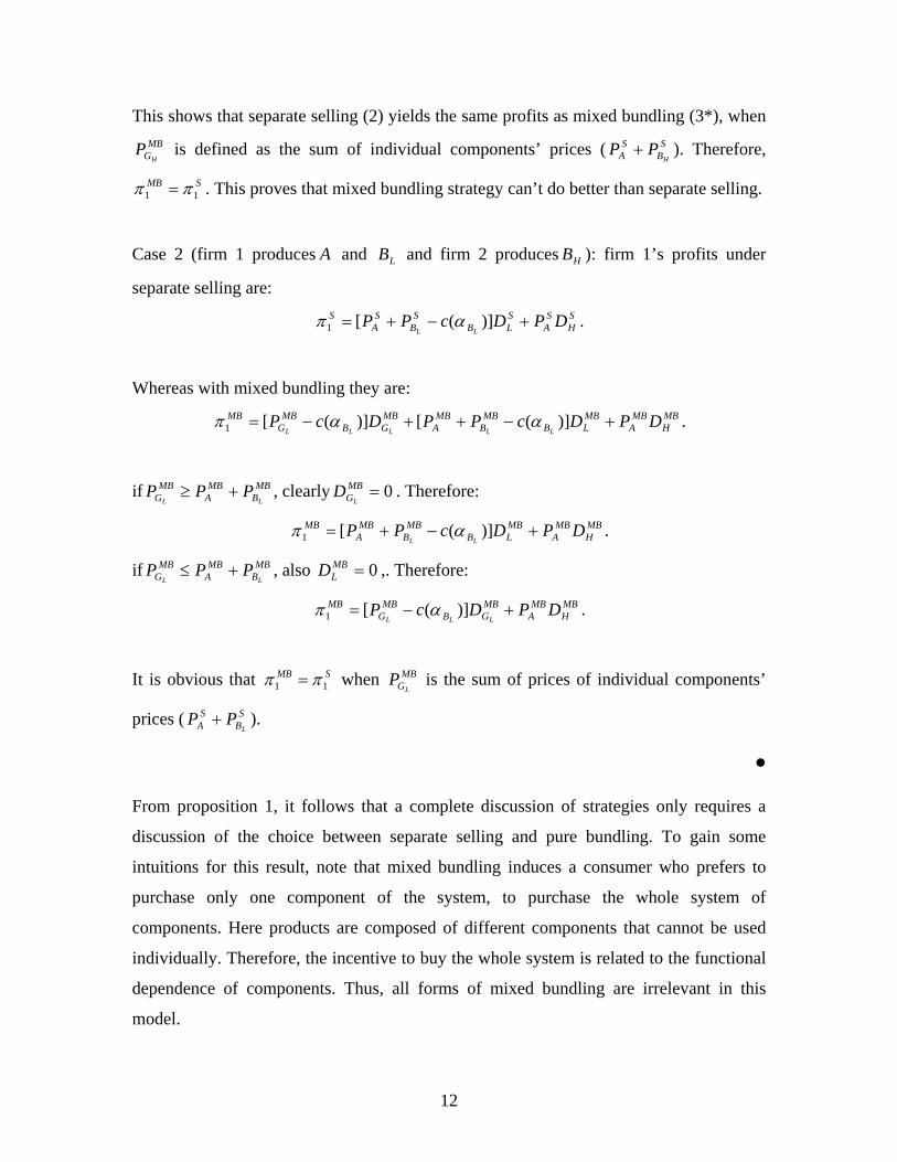
This shows that separate selling (2) yields the same profits as mixed bundling (3*), when MB

GHP is defined as the sum of individual components’ prices ( S

BS

A HPP + ). Therefore,

SMB11 ππ = . This proves that mixed bundling strategy can’t do better than separate selling.

Case 2 (firm 1 produces A and LB and firm 2 produces HB ): firm 1’s profits under

separate selling are: SH

SA

SLB

SB

SA

S DPDcPPLL

+−+= )]([1 απ .

Whereas with mixed bundling they are: MBH

MBA

MBLB

MBB

MBA

MBGB

MBG

MB DPDcPPDcPLLLLL

+−++−= )]([)]([1 ααπ .

if MBB

MBA

MBG LL

PPP +≥ , clearly 0=MBGL

D . Therefore:

MBH

MBA

MBLB

MBB

MBA

MB DPDcPPLL

+−+= )]([1 απ .

if MBB

MBA

MBG LL

PPP +≤ , also 0=MBLD ,. Therefore:

MBH

MBA

MBGB

MBG

MB DPDcPLLL+−= )]([1 απ .

It is obvious that SMB11 ππ = when MB

GLP is the sum of prices of individual components’

prices ( SB

SA L

PP + ).

•

From proposition 1, it follows that a complete discussion of strategies only requires a

discussion of the choice between separate selling and pure bundling. To gain some

intuitions for this result, note that mixed bundling induces a consumer who prefers to

purchase only one component of the system, to purchase the whole system of

components. Here products are composed of different components that cannot be used

individually. Therefore, the incentive to buy the whole system is related to the functional

dependence of components. Thus, all forms of mixed bundling are irrelevant in this

model.

13

IV. Choosing a Selling Strategy

We now characterize, for case 1 and case 2, the model’s equilibrium with separate

selling, and develop the comparison with that arising with bundling.

IV.1 Case 1: the producer of A also produces HB

Separate selling

When firm 1 sells A and HB separately, there are two available systems in the market,

HAB and LAB . Since the demands for HAB and LAB are HD , and LD respectively, the

profits under separate pricing are given for firm 1 by:

LAHBBAS DPDcPP

HH+−+= )]([1 απ , (2)

And for firm 2 by:

LBBS DcP

LL)]([2 απ −= . (4)

Firms choose prices to maximize their profits (2) and (4). We have the following first-

order conditions for firm 1:

0)]([1 =∂∂

+∂∂

−++=∂∂

A

LA

A

HBBAH

A

S

PDP

PDcPPD

P HHα

π ,

0)]([1 =∂∂

+∂∂

−++=∂∂

HH

HH

H B

LA

B

HBBAH

B

S

PD

PPD

cPPDP

απ .

And for firm 2:

0)]([2 =∂∂

−+=∂∂

L

LL

L B

LBBL

B

S

PD

cPDP

απ .

From these conditions, we obtain:

H

HLLHLH

B

BBBBBBSA

ccP

ααααααα

6)()(23 −−

= , (5)

14

H

HLHLHHLHL

B

BBBBBBBBBSBh

cccP

αααααααααα

6)(33)(2)(3)( 2+−++

= , (6)

H

LHHL

B

BBBBSBl

ccP

ααααα

3)(2)( +

= . (7)

By substituting these equilibrium prices back into profits functions, we obtain for each

firm the following level of profits:

SL

B

BBBBSH

BBS Dcc

Dc

H

HLLLHH ]6

)(2

)(2

[2

)(1 α

ααααααπ −−+

−= , (8)

SL

BBS Dc

LL

2)(

2

ααπ

−= . (9)

These results differ from the standard model of vertically differentiated duopoly. In our

model, firm 1 sells A to all consumers and sells HB to those with high reservation prices

for B . While firm 2 sells LB to consumers with low reservation prices for B . These

consumers also purchase A . Therefore the willingness of firm 1 to capture its rival’s

consumers is limited since it loses component A ’s consumers. Firm 1 prices its

components such that rival in market B cannot capture enough surplus of component B’s

consumers, then it extracts all remaining surplus in the market A , where it is monopoly.

Also, in contrast to a single integrated firm providing both components, firm 1 raises the

price of A and lowers the price of HB to induce firm 2 to lower the price of LB . Firm 1

does not engage in such practice to sell more of B , but instead to increase the demand

of A .

Pure bundling

Now assume that firm 1 bundles A and HB . Under this strategy no one purchases LB .

Therefore, this is a way to exclude firm 2 from the market. Only the system HAB is

available at priceHGP . Thus firm 1’s profits are:

15

HHH GBG

PB DcP ˆ)]([1 απ −= , (10)

where HGHD θ̂1ˆ −= , with

H

H

B

GH

Pα

θ =ˆ .

Hθ̂ represents the preference parameter of a consumer who is indifferent between

purchasing the bundle HAB and not purchasing.

The first- order condition is:

0ˆ

)]([ˆ1 =∂

∂−+=

∂∂

H

H

HHH

H G

GBGG

G

PB

PD

cPDP

απ .

The equilibrium price and profit are:

2)(

HH

H

BBPBG

cP

αα += , (11)

2

1 4)]([

H

HH

B

BBPB cα

ααπ

−= . (12)

Observe that the price of the bundle (11) is the sum of (5) and (6), which are the prices of

the individual components of the bundle when firm 1 sells its components separately. In

fact, the decision to bundle does not affect the systems’ prices given the qualities. The

intuition is that, there is no need to offer a discount to the consumers who purchase the

whole system from firm 1. The reasons are: (i) components are perfectly positively

correlated in value; and (ii) components are differentiated in quality.

Separate selling vs. pure bundling

To see whether separate selling or bundling is more profitable for firm 1, we must

compare (8) to (12).

Proposition 2: If the monopolist produces the higher quality version of B , then he earns

higher profits from separate selling than from bundling.

16

Proof

Under separate selling firm 1’s profits are:

)~()~1)](([)]([1 θθθααπ −+−−+=+−+= ABS

BS

ASL

SA

SHB

SB

SA

S PcPPDPDcPPHHHH

. (2)

While under bundling its profits are:

)ˆ1)](([ˆ)]([1 HBPB

GPBGB

PBG

PBHHHHH

cPDcP θααπ −−=−= . (10)

We can rewrite this latter function as:

)ˆ~)](([)~1)](([)ˆ1)](([1 HBPB

GBPB

GHBPB

GPB

HHHHHHcPcPcP θθαθαθαπ −−+−−=−−= . (10*)

Since PBG

SB

SA HH

PPP =+ , the first terms of (2) and (10*) are equal. Then to compare

S1π to PB

1π , we have just to compare the last term of (2), )~( θθ −SAP to the one of (10*),

)ˆ~)](([ HBPB

G HHcP θθα −− .When we compute these two terms, we find that the former can

be written as:

])(3

)()([)~(

LHL

LHHL

BBB

BBBBSA

SA

ccPP

ααααααα

θθ−

−=− .

While the latter is:

])(3

)()()][([)ˆ~)](([

LHH

LHHL

HHHHBBB

BBBBB

PBGHB

PBG

cccPcP

ααααααα

αθθα−

−−=−− .

Therefore separate selling is better than bundling if and only if:

)~( θθ −SAP > )ˆ~)](([ HB

PBG HH

cP θθα −−H

L

HHB

BB

PBG

SA cPP

αα

α )]([ −>⇔ .

As PBG

SB

SA HH

PPP =+ , we have:

)~( θθ −SAP > )ˆ~)](([ HB

PBG HH

cP θθα −− 03

)()(>

−⇔

L

LHHL

B

BBBB ccα

αααα.

Since 0)()( >−LHHL BBBB cc αααα , we have PBS

11 ππ > .

17

•

Bundling Buy: nothing HAB

--------------------------------------______________________

Hθ̂

0 θ θ~ 1 …………………..-------------------------------____________

Separate Selling Buy: nothing LAB HAB

]1,0[~ Uθ

Figure 2

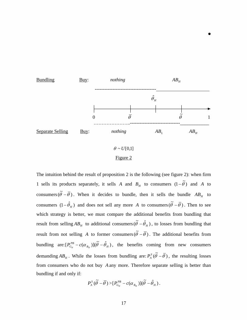
The intuition behind the result of proposition 2 is the following (see figure 2): when firm

1 sells its products separately, it sells A and HB to consumers )~1( θ− and A to

consumers )~( θθ − . When it decides to bundle, then it sells the bundle HAB to

consumers )ˆ1( Hθ− and does not sell any more A to consumers )~( θθ − . Then to see

which strategy is better, we must compare the additional benefits from bundling that

result from selling HAB to additional consumers )ˆ~( Hθθ − , to losses from bundling that

result from not selling A to former consumers )~( θθ − . The additional benefits from

bundling are: )ˆ~)](([ HBPB

G HHcP θθα −− , the benefits coming from new consumers

demanding HAB . While the losses from bundling are: )~( θθ −SAP , the resulting losses

from consumers who do not buy A any more. Therefore separate selling is better than

bundling if and only if:

)~( θθ −SAP > )ˆ~)](([ HB

PBG HH

cP θθα −− .

18

This is the case when the production cost is convex: 0)()( >−LHHL BBBB cc αααα . Here the

result of bundling is a narrowing of market since consumers )ˆ( θθ −H who bought the

system of lower quality dot not buy under bundling.

IV.2 Case 2: the producer of A also produces LB .

Separate selling

When firm 1 sells A and LB separately, the profits of firm 1 and firm 2 are respectively

given by:

HALBBAS DPDcPP

LL+−+= )]([1 απ , (13)

HBBS DcP

HH)]([2 απ −= . (14)

And equilibrium prices are:

6)()(22

LHLH BBBBSA

ccP

αααα −−+= , (15)

3)()(2

HLLH

H

BBBBSB

ccP

αααα +−+= , (16)

3)(2)(

LHLH

L

BBBBSB

ccP

αααα +−+= . (17)

We observe that the price of A is higher and the prices of HB and LB are lower compared

to the case where the monopolist produces HB . This comes to the fact that firm 1

increases the price of A to capture more surplus of consumers with high reservation

prices for system HAB . Therefore the prices of strategic substitute, HB and LB , decrease.

Here there is much more surplus to capture in the market of B .

By substituting (15), (16) and (17) into the profit functions (13) and (14), we obtain:

19

SL

BBSH

BBBBS Dc

Dcc

LLLLLH ]2

)([]

6)()(22

[1

ααααααπ

−+

−−+= , (18)

SH

BBS Dc

HH ]2

)([2

ααπ

−= . (19)

In comparison to case 1, we find that firm 1’s profits are lower while firm 2’s profits are

higher. This is because now firm 2 serves the high reservation price consumers of B ,

which is the most profitable segment of the market.

Pure bundling

If firm 1 bundles, its profits are:

LLL GBGPB DcP ˆ)]([1 απ −= , (20)

where LGLD θ̂1ˆ −= with

L

L

B

GL

Pα

θ =ˆ ,

where Lθ̂ is the preference parameter of a consumer indifferent between purchasing

bundle LAB and not purchasing.

Since there is compatibility, the consumers who desire to purchase the higher quality

system HAB , must purchase HB in addition to bundle LAB . They will do so if:

LLHLH GBBGB PPP −≥−− θαθα . (21)

If we denote by *Hθ , the preference parameter of an indifferent consumer between

purchasing HB in addition to the bundle LAB to form the higher quality bundle HAB and

the lower bundle LAB alone, we obtain from (21):

LH

H

BB

BH

Pαα

θ−

=* . (22)

Consequently the demand for the higher quality bundle HAB is:

** 1 HHD θ−= .

This gives firm 2’s profits as: *

2 )]([ HBBPB DcP

HHαπ −= . (23)

20

By maximizing (20) and (23) with respect to prices, one obtains:

2)(

LL

L

BBPBG

cP

αα += , (24)

2)(

HLH

H

BBBPBB

cP

ααα +−= . (25)

From (25), we can rewrite *Hθ as:

)(2)(

21*

LH

H

LH

H

BB

B

BB

PBB

H

cPαα

ααα

θ−

+=−

= . (26)

We have 10 * ≤≤ Hθ , i.e.:

)(1)(2

)(21

HLH

LH

HBBB

BB

B cc

ααααα

α≥−⇔≤

−+ . (27)

Condition (27) is the constraint for firm 2 to remain in the market. Firm 2 sells HB if and

only if the difference of reliability between HB and LB is greater than the unit production

cost of HB . Otherwise all consumers prefer to purchase the bundle of lower quality LAB

(i.e. nobody will purchase HB in addition). Equilibrium profits for firm 1 and firm 2 are

respectively:

2

1 4)]([

L

LL

B

BBPB cα

ααπ

−= , (28)

⎪⎩

⎪⎨⎧ ≥−

−

−−=

=

)()(4

)]([

0

2

2

2

HBLBHBLBHB

HBLBHBPB

PB

cifc

else

ααααα

αααπ

π

Separate selling vs. pure bundling

The ranking of profits for the monopolist (firm 1) is summarized in the following

proposition.

21

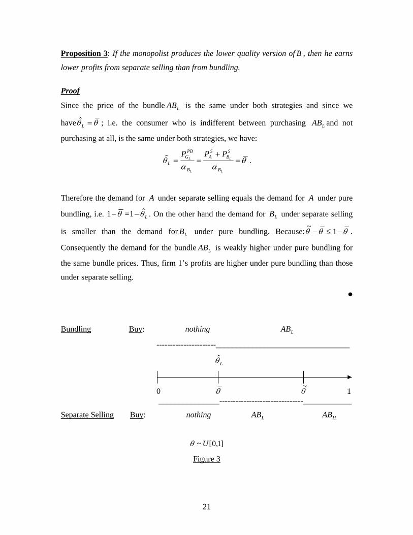
Proposition 3: If the monopolist produces the lower quality version of B , then he earns

lower profits from separate selling than from bundling.

Proof

Since the price of the bundle LAB is the same under both strategies and since we

have θθ =Lˆ ; i.e. the consumer who is indifferent between purchasing LAB and not

purchasing at all, is the same under both strategies, we have:

θαα

θ =+

==L

L

L

L

B

SB

SA

B

PBG

L

PPPˆ .

Therefore the demand for A under separate selling equals the demand for A under pure

bundling, i.e. θ−1 = Lθ̂1− . On the other hand the demand for LB under separate selling

is smaller than the demand for LB under pure bundling. Because: ≤−θθ~ θ−1 .

Consequently the demand for the bundle LAB is weakly higher under pure bundling for

the same bundle prices. Thus, firm 1’s profits are higher under pure bundling than those

under separate selling.

•

Bundling Buy: nothing LAB

----------------------_________________________________

Lθ̂

0 θ θ~ 1 _______________-------------------------------____________

Separate Selling Buy: nothing LAB HAB

]1,0[~ Uθ

Figure 3

22

For proposition 3, the intuition is simple (see figure 3). The price of the bundle is the

same under both regimes and demands under pure bundling are greater than demands

under separate selling. Therefore for firm 1, bundling is better than separate selling. We

found a case where bundling is a profitable strategy and can lead to foreclosure and

exclusion of the rival from the market.

To sum up, firm 1 who is monopolist on A never finds it worthwhile to bundle in order

to reduce the level of competition in market for B when the result of bundling is a

narrowing of market for its monopolized component. The reason lies in the fact that since

the monopolized product A is essential for all uses of products B ( HB and LB ), the

monopolist can benefit from competition in B through sales of its monopolized

product A with separate selling. This is the case when the monopolist of A

produces HB .Therefore he prefers separate selling over bundling. On the other hand when

the monopolist of A produces LB , separate selling brings no increase in the demand for

its monopolized product A and even reduces the demand for its product LB through

competition with HB . Therefore, separate selling is dominated by bundling.

Corollary 1: The monopolist will sell its products separately if and only if its product B

has the higher quality.

Whinston (1990) and Matutes and Regibeau (1992) stated that if firms sell compatible

components, then bundling is dominated by separate selling. The set up of Whinston

(1990) is same as here except that: (i) he considers the case of technical bundling; and (ii)

he does not consider products differentiated in quality. In the model of Matutes and

Regibeau (1992), no firm has a monopoly over either component and products are

horizontally differentiated. Therefore our results cannot be directly compared to their

results. However, our results extend theirs to the case where components are vertically

differentiated.7’8

7 Our results are also in contrast to Choi (2003) who demonstrated in asymmetric information setting that a monopolist will choose to bundle a product of established quality to one of unknown quality by consumers only if for the latter the monopolist produces a quality higher than rivals’.

23

IV.3 Welfare Analysis

Now let us see how consumers’ surplus and social welfare are affected by bundling

decision. When firm 1 sells its components separately, consumers’ surplus denoted by SCS is:

θθαθθαθ

θθ

dPdPCS SABB

SABB

SLLHH)()(

~1

~−+−= ∫∫ .

While the social welfare denote by SSW is: SSSS CSSW 21 ππ ++= .

When bundling is allowed consumers’ surplus )( PBCS is:

∫ −=1

ˆ

)(i

iidPCS PB

GBPBi

θ

θθα )ˆ1(2

)ˆ1( 2

iPB

GBi

iiP θα

θ−−

−= , { }LHi ,∈ .

And the social welfare )( PBSW is: PBPBPB

iPB

i CSSW 21 ππ ++= , { }LHi ,∈ .

Proposition 4: Consumers’ surplus and social welfare are always higher under separate

selling than under pure bundling.

Proof

Intuitively for case 1 (firm 1 produces A and HB , whereas firm 2 produces LB ), pure

bundling increases the number of consumers of HAB from )~1( θ− to )ˆ1( Hθ− and

eliminates )~( θθ − of consumers of LAB (see figure 2). Therefore, consumers’ surplus

under pure bundling is greater than under separate selling if and only if the additional

surplus obtained by new consumers of HAB , )ˆ~( Hθθ − when consuming the higher quality

under bundling (rather than the lower quality under separate selling) is lower than the

8 Remark that when costs of quality improvement are fixed, the result is easily deductible. The monopolist chooses bundling such to foreclose its competitor in B . Indeed, as proved by Diallo (2004), for symmetrical distribution of consumers’ taste for quality, the monopolist prefers to produce only one variety of a system when costs of quality improvement are fixed. So he would like to eliminate the others varieties from the market.

24

losses of surplus of consumers )~( θθ − who do not consume LAB under pure bundling.

Formally we have PBH

S CSCS ≥ if:

∫∫ −≥−−−θ

θ

θ

θ

θθαθθαα~~

ˆ

)()]()[( dPdPP SABB

SAB

PBGBB LL

H

LHLH. (29)

After computation we obtain the following condition for (29) to be true:

0)( 2 ≥− SABB

PBGB LLHH

PP αα .

Thus, consumers’ surplus is higher under separate selling than under pure bundling. Since

this is also true for firms’ profits, this is true for social welfare.

For case 2 (firm 1 produces A and LB , whereas firm 2 produces HB ), the result is

straightforward. Indeed by bundling, )~1( θ− consumers purchase LAB instead of HAB .

This reduces the surplus of these consumers who had higher surplus with HAB . At the

same time, the surplus of consumers )~( θθ − does not change since prices and qualities

are identical (see figure 3). Consequently consumer surplus decreases under bundling.

Also, under bundling firm 2’s losses (not to sell HB ) exceed firm 1’s additional benefits

(sell more LB ). Since firms’ profits also decrease under bundling, immediately social

welfare also decrease under bundling.

•

IV.4 Numerical Application with Endogenous Quality Choice

We consider now a game where firms compete in two-stages. In the first stage, the

monopolist chooses its marketing strategy (bundling or not) and the two firms

simultaneously choose their quality levels. In the second they concurrently determine

prices- given the qualities and strategy already chosen- and produce the output which

25

satisfies consumers’ demands. A solution of this game consists of a set of equilibrium

quality and pricing decisions for each firm. We focus on subgame perfect Nash

equilibria. We also assume that the marginal cost of production is quadratic, i.e.:

2)()(

2αα =c .

Since quality is endogenous both firms may choose the same quality for B . If firm 1 does

not bundle then Bertrand competition leads to a unique equilibrium where prices equal

unit cost. Hence, both firms make zero profits. Therefore, firm 2 produces a

component B differentiated in quality from firm 1’s under separate selling and bundling.

From the previous results we know that the only certain equilibrium with two active firms

is where firm 1 produces the higher quality of B . In that situation it sells its components

separately (otherwise it bundles its components and this can exclude firm 2). Then the

profits are given by (2) for firm 1 and by (4) for firm 2. With a quadratic cost function,

we rewrite these profits as:

LAHB

BAS DPDPP H

H+−+= ]

2)(

[2

1

απ , (30)

LB

BS DP L

L]

2)(

[2

2

απ −= . (31)

For any given pair of reliability, maximizing (30) and (31) with respect to prices, gives

the following equilibrium prices:

12)(26 2

HLLL BBBBSAP

αααα −−= , (32)

12)(36)(26 22

HHLLHH

H

BBBBBBSBP

αααααα ++−+= , (33)

6)2(

HLL

L

BBBSBP

ααα += . (34)

By the first derivatives in quality, we observe that SAP is decreasing in

HBα and

increasing inLBα , S

BhP is increasing in HBα and decreasing in

LBα and SBL

P is increasing in

26

HBα andLBα . These variations suggest that for firm 1 to induce firm 2 to lower the price

of LB , it must choose HBα as close as possible to

LBα . Also, we know that SBL

P is

increasing inLBα ; this implies that the quality dispersion (difference of qualities) will be

lower under this market structure compared to the traditional model of duopoly in a

Mussa and Rosen (1978) framework.

We look now for the solution of the quality game. Firms choose their quality

specification to maximize their profits (30) and (31). By substituting the equilibrium

prices (32), (33), and (34) back into profit functions, and maximizing these latter

functions with respect to qualities, we get a nonlinear system of equations

of ),(LH BB αα which is solved numerically to obtain the following Bα s:

710102.0=SBH

α , (35)

35505.0=SBL

α . (36)

Equilibrium prices and profits for separated selling are therefore:

1355.0=SAP ; 3456.0=S

BHP ; 08404.0=S

BLP

076329.01 =Sπ ; 002486.02 =Sπ .

Expressions (35) and (36) give the pair of candidate equilibrium qualities. The second

derivatives with respect to qualities given the equilibrium qualities are negative:

02139.0)( 71010.02

12

≤−=∂∂

=LB

HB

S

ααπ and 00394.0

)( 35505.022

2

≤−=∂∂

=LB

LB

S

ααπ .

However, that shows only that (35) and (36) represent a local maximum. This is not

enough to ensure we have found a Nash equilibrium. To be sure that our candidate

maximum is indeed an equilibrium we also have to check first that firm 2 has no

incentive to “leapfrog” firm 1 and itself produce the highest quality and second that firm

1 makes more profits as a monopolist in A and a duopolist producing HB than as a

monopolist in both markets A and B .

27

If firm 2 produces its component B at a quality level above the one of firm 1, we know

that the best strategy of firm 1 would be bundling. We show that in this case firm 2

makes zero or less profits than before “leapfrogging”. After “leapfrogging” firm 1 profits

are given by:

LLL GBGPB DcP ˆ)]([1 απ −= . (37)

After optimization of (37), we obtain easily the following results for equilibrium quality,

price and profits:

6666.0=PBBL

α ; 44444.0=PBGL

P ; 07407.01 =PBπ .

Since 1π is concave in quality, by showing that 0)( 21

2

<∂∂

Bαπ , is a sufficient condition for

6666.0=PBBα being a global maximum. That is the case since 01

)( 6666.021

2

≤−=∂∂

=BhBh

S

ααπ .

For firm 2, its profits are:

⎪⎪⎩

⎪⎪⎨

⎧≥−

−

−−=

=

)38(2

)()(4

]2

)([

0

222

2

2

HBLBHB

LBHB

HBLBHB

PB

PB

if

else

ααα

αα

ααα

π

π

Under the constraints:LH BB αα ≥≥1 and 6666.0=PB

BLα , there is no solution PB

BHα which

satisfies 2

)( 2PBBPB

BPBB

H

LH

ααα ≥− for the maximization of (38) with respect to qualities.

Therefore, we have 02 =PBπ .

Now we must check whether firm 1 makes more profits as a duopolist producing HB

than as a monopolist in B . It is straightforward that firm 1’s profits under separate selling

are higher than those under bundling since:

076329.01 =Sπ PB107407.0 π=> .

28

Corollary 2: The monopolist will always produce the higher quality of B in a dynamic

game.

Thus, the outcome of the subgame perfect Nash equilibrium is such that firm 1 selects SBH

α equals to 710102.0 , and firm 2 selects SBL

α equals to 35505.0 .9 SBL

α is half of SBH

α

and their difference equals to 35505.0 . When we determine quality choice in a standard

model of duopoly in a Mussa and Rosen (1978) framework, we obtain that DBH

α equals to

8195.0 and DBL

α equals to 3987.0 ; their difference equals to 4208.0 .

Since 4208.0 is greater than 35505.0 , immediately we deduce that the spread of

component B quality in our market structure outcome is too low relative to the standard

profit maximization duopoly outcome. The reason is that the monopolist want to extract

more surplus in market A from intensifying price competition in market B. He achieves

that by not differentiate its component B from rival’s. Consequently, quality

differentiation in market B between the firms is tighter and price competition is

intensified.

V. Antitrust Implications and Conclusion

We analyzed bundling incentives in markets where products are composed of two

complementary components. One of the components is monopolized and the other is sold

by a duopoly. We assumed quality differentiation between components. We developed a

model of quality competition and we demonstrated the monopolist’s bundling decision

depends on the quality level of the component where he faces competition. We proved

that if the monopolist’s component has a quality higher than the competitor’s then the

monopolist prefers not to bundle. On the other hand if the quality of this component is

9 When we compute consumers’ surplus and social welfare under both marketing strategies, we find that:

038165.0=SCS ; 03703.0=PBCS ; 117.0=SSW ; 111.0=PBSW

As proved in the preceding section, consumers’ surplus and social welfare are higher under separate selling than pure bundling.

29

lower than the competitor’s then the monopolist prefers bundling. For the monopolist the

incentive not to bundle is related to market extensions for its monopolized component.

He chooses the marketing strategy which helps to achieve this goal. Consequently it may

appear a possible exclusion or foreclosure of competitor. Thus, we showed that this is an

exclusionary bundling. However, when we look for the subgame perfect Nash

equilibrium, we found that the monopolist chooses to produce the higher quality of the

complementary product and separate selling is its best strategy.

The results of this paper, which show that bundling could be anticompetitive can be used

to asses a proper legal rule regarding bundling in market for complementary components

when quality matters. For example in the Microsoft litigation courts have had to

determine whether it was lawful for Microsoft to bundle its Internet Explorer browser

with Windows operating system. Since Microsoft is almost a monopoly in the personal

computer operating system, faces competition in the browser market essentially from

Netscape and both products are complementary, this case fits appropriately our model if

we consider the two web browsers to be quality differentiated. Absent the possibility that

the complementary component, Netscape Navigator might later in the future become a

substitute to Windows, the presence of network externality, and predatory pricing, our

results suggest that the bundling strategy adopted by Microsoft implies that Internet

Explorer is of lower quality than Netscape Navigator and that Microsoft leverage its

market power from the operating system market to the web browser market.

In most of the studies on bundling there is no clear cut about welfare effects of bundling.

We found that the welfare effects of bundling are clearly negative. This establishes that

an efficiency presumption of bundling in markets where products are composed of two

strictly complementary components, with market power in one component is

unwarranted. This suggests a prohibition per se of bundling in these types of markets.

In an imperfect and asymmetric information world, bundling may also be a signal for bad

quality of the monopolist’s complementary product. It is worthwhile to note that the

results of this paper must be interpreted under the following simplifications: we ignored

30

positive demand externalities (or network externalities) and we assumed no cost savings

result from bundling. Network externalities will increase the profitability of separate

selling, while cost savings that result from economy of scope in distribution will increase

the profitability of bundling. Finally, for future research, it will be interesting to look at

the case where each firm supplied all the components necessary to form the complete

system.

References

Adams, W. James. and Yellen, Janet L., 1976, “Commodity Bundling and the Burden

of Monopoly,” Quarterly Journal of Economics, 90, 475 –98.

Director, A. and Levi, Edward, 1956, “Law and the Future: Trade Regulation,” North-

western University Law Review, 51, 281 –96.

Bork, Robert H., 1978, “The Antitrust Paradox,” New York: Basic Books.

Burstein, Meyer L., 1960, “The economics of Tie-in Sales,” Review of Economics and

Statistics, February, 42, 68-73.

Carbajo, J., De Meza, D. and Seidman, DJ., 1990, “A strategic motivation for

commodity bundling,” Journal of Industrial Economics, 38, 458-486.

Chou, C., and Oz. Shy, 1990, “Network Effects Without Network Externalities,”

International Journal of Industrial Organization, 8, 259-270.

Choi, J, Pil, 2003, “Bundling new products with old to signal quality, with application to

The sequencing of new products,” International Journal of Industrial

Organization, 21, 1179-1200.

Crampes, Claude and Abraham Hollander, 1995, “Duopoly and quality standards,”

European Economic Review, 39, 71-82.

Diallo, Thierno, 2004, “Horizontal Mergers, Quality Choice, and Welfare,” mimeo,

Université de Montréal.

Economides, Nicholas, 1989, “Desirability of Compatibility in the Absence of Network

Externalities,” American Economic Review, 79, 747-789.

Economides, Nicholas, 1991, “Compatibility and Market Structure,” Discussion Paper

Stern School of Business, N.Y.U.

31

Economides, Nicholas, 1993, “Mixed Bundling in Duopoly. Stern School of Business,”

working paper, Stern School of Business, N.Y.U.

Economides, Nicholas and William Lehr, 1994, “The Quality of Complex Systems and

Industry Structure,” in William Lehr (ed.), Quality and Reliability of

Telecommunications Infrastructure, Lawrence Erlbaum, Hillsdale.

Einhorn, Michael A., 1992, “Mix and Match Compatibility with Vertical Product

Dimensions,” The Rand Journal of Economics, 23, 535-547.

Gabszewicz J.J and J.-F. Thisse, 1979, “Price Competition, Quality, and Income

Disparities,” Journal of Economic Theory, 20, 340-359.

Matutes, Carmen and Regibeau, Pierre, 1992, “Compatibility and Bundling of

Complementary Goods in a Duopoly,” Journal of Industrial Economics, 40,37-54.

McAfee .R. Preston, McMillan, John, and Whinston, Michael D, 1989, “Multiproduct

Monopoly, Commodity Bundling, and Correlation of Values,” Quarterly Journal

of Economics, 84, 271 –284.

Mussa, Michael and Sherwin Rosen, 1978, “Monopoly and Product Quality,” Journal

of Economic Theory, 18, 301-317.

Nalebuff, Barry, 2004, “Bundling As En Entry Barrier,” Quarterly Journal of

Economics, 104, 371 –84.

Posner, Richard A., 1976, “Antitrust Law: An Economic Perspective,” Chicago:

University of Chicago Press.

Salinger, Michael A., 1995, “A Graphical Analysis of Bundling,” Journal of Business,

68, 85 –98.

Schmalensee, Richard, 1982, “Commodity Bundling by Single-Product Monopolies,”

Journal of Law and Economics, 25, 67 –71.

Schmalensee, Richard, 1984, “Gaussian Demand and Commodity Bundling,” Journal of

Business, 57, 58 –73.

Tirole, Jean, 1988, “The Theory of Industrial Organization,” The MIT Press.

Stigler, Georges. J, 1968, “A Note on Block Booking,” In G.J Stigler, ed., The Theory

of Industry, Chicago: University of Chicago Press.

Whinston, Michael .D., 1990, “Tying Foreclosure, and Exclusion,” American Economic

Review 80, 837 –59.