Embed Size (px)
Citation preview

Does the term structure of corporate interest
rates predict business cycle turning points?
Jordan Fixler
Senior Thesis
Advisor: Ben Eden

Abstract
The Treasury Yield Curve has been a very accurate leading economic indicator
for the past 60 years—though normally sloping upward, it has inverted prior to every
recession in that time period with only two false alarms. Even in those two cases, marked
slowdowns in economic activity followed the inversions within the standard time period
of four to six quarters. Despite the consistency, economists have not developed a widely
accepted theory as to how this term structure of interest rates is able to predict business
cycle turning points. This paper looks at term structures derived from corporate interest
rates in an effort to compare them to that of the Treasury, with the hopes of shedding
some light on their predictive ability. Through the use of various regressions, the paper
finds that corporate interest rates are not as successful at predicting recession as Treasury
interest rates. The paper then hypothesizes that the reasoning for this difference has to do
with the government’s role in the Treasury security market and/or Treasury securities’
“risk-free” designation.

Table of Contents
1 Introduction.......................................................................................................................1
1.1 The Yield Curve.........................................................................................................1
1.2 Corporate Debt...........................................................................................................4
2 Characteristics of Bonds ...................................................................................................5
2.1 Bond Pricing and Markets .........................................................................................5
2.2 Bond Theories............................................................................................................7
2.3 Theoretical Basis for Thesis.......................................................................................9
3 Data .................................................................................................................................11
3.1 Bond Data ................................................................................................................11
3.2 Recession Data.........................................................................................................13
4 Empirical Implementation ..............................................................................................15
4.1 Ordinary Least Squares Regression .........................................................................15
4.2 Multiple Regression .................................................................................................17
4.3 Probit Regression .....................................................................................................19
5 Conclusion ......................................................................................................................20
5.1 Discussion of Results...............................................................................................20
5.2 Direction for Further Research ................................................................................23
Bibliography……….…………………………………………………………………..25
“Predicting the future has always fascinated humans, and economic forecasting doubles
the interest by adding a chance to turn profit.”
- Joseph Haubrich, Federal Reserve Bank of Cleveland1
1 Haubrich, Joseph. “Does the Yield Curve Signal Recession?” Federal Reserve Bank of
Cleveland. Pg. 1.
1
1 Introduction
1.1 The Yield Curve
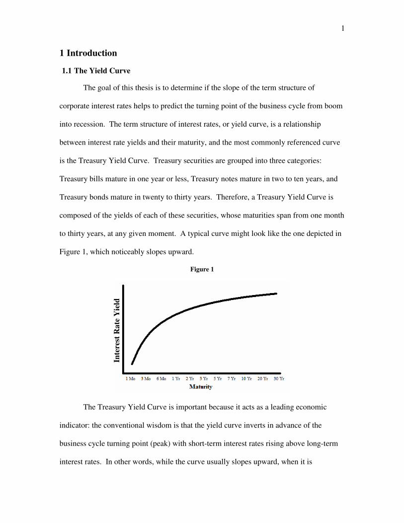
The goal of this thesis is to determine if the slope of the term structure of
corporate interest rates helps to predict the turning point of the business cycle from boom
into recession. The term structure of interest rates, or yield curve, is a relationship
between interest rate yields and their maturity, and the most commonly referenced curve
is the Treasury Yield Curve. Treasury securities are grouped into three categories:
Treasury bills mature in one year or less, Treasury notes mature in two to ten years, and
Treasury bonds mature in twenty to thirty years. Therefore, a Treasury Yield Curve is
composed of the yields of each of these securities, whose maturities span from one month
to thirty years, at any given moment. A typical curve might look like the one depicted in
Figure 1, which noticeably slopes upward.
Figure 1
The Treasury Yield Curve is important because it acts as a leading economic
indicator: the conventional wisdom is that the yield curve inverts in advance of the
business cycle turning point (peak) with short-term interest rates rising above long-term
interest rates. In other words, while the curve usually slopes upward, when it is
Inte
rest
Ra
te Y
ield

2
downward sloping, or “inverted,” a recession generally begins sometime in the following
four to six quarters.2 For example, Figure 2 is a snapshot of the inverted Treasury Yield
Curve as of August 19,2006, which preceded by five quarters the recession beginning in
December 2007 (as defined by the National Bureau of Economic Research3). Figure 3
bears out the historical relationship between yield curve inversions, as measured by the
spread between the ten year Treasury bill and three month Treasury note rates, and the
quarterly percent change in Gross Domestic Product, as measured by the Bureau of
Economic Analysis. This spread, and the ten year to two year spread, are the most
common measures of the shape of the yield curve, and an inversion is defined as a spread
less than or equal to zero. Figure 3 shows that since 1960, the Treasury Yield Curve has
inverted eight times, and seven of those times a recession followed. The exception, an
inversion in 1966, was still followed by a “credit crunch” and decline in production later
that year.
Figure 2
Yield curve. Source: Bloomberg. Accessed 11/9/09 at
http://www.econbrowser.com/archives/2006/08/the_yield_curve_1.html
2 Estrella, Arturo. “The Yield Curve as a Leading Indicator: Frequently Asked
Questions.” October 2005. Pg. 2. 3 National Bureau of Economic Research. Determination of the December 2007 Peak in
Economic Activity. http://www.nber.org/cycles/dec2008.pdf

3
Figure 3
Yield Curve vs Real GDP Growth
-15.00
-10.00
-5.00
0.00
5.00
10.00
15.00
20.00
Apr-
53
Apr-
56
Apr-
59
Apr-
62
Apr-
65
Apr-
68
Apr-
71
Apr-
74
Apr-
77
Apr-
80
Apr-
83
Apr-
86
Apr-
89
Apr-
92
Apr-
95
Apr-
98
Apr-
01
Apr-
04
Apr-
07
Date
Pe
rce
nt
Ten Year Minus Three
Month Treasury Spread
Quarterly % Change in
GDP
Two questions arise upon reviewing this data: what is the significance of an
economic leading indicator, and why is the curve proved to be such an accurate one? To
the first question, the forecasting power of the yield curve is of interest to those in the
fields of economics, finance, and perhaps even psychology. The ability to predict
oncoming recessions would be beneficial to the field of economics in that fiscal and
monetary policy are more effective the sooner they are implemented, and conceivably
could be used to avoid recessions or lower their negative impact. Those in finance would
welcome an accurate, well understood predictor for business cycles so that they could
better time their investments and earn higher profits. Psychologists would be interested
in the aspect of market expectations, which is the basis for the most widely accepted
theory that explains the Treasury Yield Curve’s behavior. The second question remains
to be unanswered, and while this paper does not seek to answer it outright, it does seek to
4
add research to the debate. This paper will explore what is known about the Treasury
Yield Curve, and will try to determine if a yield curve derived from corporate interest
rates share the same power of prediction.
1.2 Corporate Debt
Corporate bonds defer from the standardized securities issued by the Treasury
Department in that they are issued by thousands of businesses with varying levels of
financial health. Therefore, corporate bonds are categorized not just by maturity
(corporate paper refers to issued debt with a maturity of 270 days or less), but also by
grades issued by ratings agencies such as Moody’s and Fitch, who analyze each
company’s health. Grades of Aaa and AAA, respectively, are the highest and mean the
associated bonds are considered the least risky, and thus generally have the lowest
interest rate.
The most important difference between Treasury and corporate debt, and the basis
for this paper, is that the corporate debt market is free from direct government influence.
Treasury security yields are affected in the primary market through the Treasury
Department’s decision of how much debt to issue at a given time, and what its maturity
will be. As part of the United States government, these decisions are influenced by
budgeting issues, but also perhaps by government initiatives to influence interest rates.
Similarly, the Federal Reserve purchases and sells Treasury securities explicitly with the
intent of influencing interest rates, so as to properly manage economic growth and
stability. That the government does not buy or sell in the primary or secondary corporate
bond market means that it ought to be a more pure form of market expectations, which as

5
previously mentioned, is the basis for the most widely accepted theory explaining the
behavior of the Treasury Yield Curve, and will be explained in the next section.
2 Characteristics of Bonds
2.1 Bond Pricing and Markets
Before moving forward, it will be useful to discuss different characteristics of
bonds, beginning with how they are priced. Bond prices are determined in a similar
fashion to most other assets—as a function of supply and demand. Suppliers issue bonds
in order to borrow money from investors, who cumulatively make up demand in a given
bond market. What is unique about the bond market is that the most relevant and often
quoted characteristic of a bond is not the price, but the interest rate. Bond prices are a
function of, and inversely related to, the interest rate, as seen in Figure 4.
Figure 4
http://www.oswego.edu/~edunne/image45.gif
Generally speaking, there are two types of bonds. Zero-coupon bonds, such as
Treasury bills are purchased at a given value and the investor is repaid a redemption
value at the end of the maturity period. The interest rate, or yield to maturity, is the rate

6
which equates the two values for the given time period. Coupon bonds, such as Treasury
notes or bonds, are also purchased at a given value and pay a redemption value at the end
of the maturity period, but also pay interest (coupon payments) in between, often two
times a year. The yield to maturity is the interest rate (not the coupon rate) that equates
all payments with the purchasing value. The differences in bond structure can be seen in
the following equations:
Zero-Coupon ( ) investment oflength
rateinterest 1
Value RedemptionPrice
+=
Coupon
Bondinvestment oflength
investment oflength
0 period time rate)interest (1
Value Redemption
rate)interest (1
PaymentCoupon Price
++
+= ∑
There are several common factors that drive supply and demand in the bond
market. Increases in investor wealth, the expected return on bonds, and the liquidity of
bonds relative to other assets result in an increase in demand. The additional wealth
means investors have more to invest, while the increased expected return and liquidity
make bonds a more attractive investment. Increases in the expected interest rate,
inflation rate, and riskiness of bonds relative to other assets decrease the demand for
bonds. Higher interest and inflation rates lower the expected return for bonds, while
added risk makes bonds a less attractive investment. On the supply side, expected
increases in economic output and inflation increase the supply of bonds, as do higher
government deficits. Economic growth yields profitable investment opportunities that
businesses want to raise money for, while inflation lowers the real cost of raising that
debt. Higher deficits lead to more bonds being issued in order to bridge budget gaps.
7
2.2 Bond Theories
Joseph Haubrich, a vice president at the Federal Reserve Bank of Cleveland,
wrote that “economists do not currently have a well-accepted theory of why the yield
curve predicts future economic growth4.” However, there are noticeable repeated
behaviors by the curve and established theories that help to explain this behavior and the
curve’s underlying components. One observation is that interest rates on bonds of
different maturities tend to move together over time. For example, if the Federal Reserve
raises the short-term interest rate target, the entire Treasury Yield Curve is likely to shift
upward, not just the short-maturity end. This can be explained by the Expectations
Theory of the term structure of interest rates, which states that the interest rate on a long-
term bond will equal an average of short-term interest rates that the market expects to
occur over the life of the long-term bond. The assumption that this theory relies on is that
bonds of different maturities are perfect substitutes in the eyes of investors, and thus the
expected returns on those bonds must be equal. Historically, if short-term rates rise,
future rates are more likely to be higher, and thus the Expectations Theory explains why
rates move together.
The Expectations Theory also explains another observation that characterizes the
Treasury Yield Curve: when short-term rates are low, the curve is more likely to slope
upward, while when they are high, the curve is more likely to slope downward. These
characteristics are a result of the market expecting low or high rates to move to a more
moderate level in the future. Intuitively, low rates are probably the result of the Federal
Reserve having a low Discount Rate and/or Federal Funds target, which often occur when
4 Haubrich, Joseph. “Does the Yield Curve Signal Recession?” Federal Reserve Bank of
Cleveland. Pg. 3.

8
the economy needs stimulating through monetary policy. Interest rates that are left too
low for too long can lead to asset bubbles or inflationary environments however, and
therefore the market expects rates to be raised in the future. Conversely, high short-term
rates are probably the result of the Federal Reserve targeting high inflation (and the
market demanding high interest payments to account for rampant inflation), but these
rates will slow down economic output and thus the market expects a return to lower rates
in the future.
A third observation is that the Treasury Yield Curve nearly always slopes upward,
except in the case of recession. Utilizing the Expectations Theory, this would mean that
interest rates are more likely to rise in the future rather than fall, whereas in reality either
is just as likely. The Segmented Markets Theory looks at the markets for bonds of
different maturities as completely separate, and thus pricing of a long-term bond is
independent of a short-term bond. The markets are segmented because investors are
assumed to have a personal preferential holding period. For example, an investor who
needs funding in three years would only be interested in the markets for bonds with
maturities of three years or less. Due to this segmentation, bonds are priced based on the
supply and demand for that specific maturity range, and generally the demand for short-
term bonds is higher than for long-term bonds. As a result, prices for short-term bonds
are higher and interest rates are lower.
All three observations are true, and yet only when the two defined theories are
combined are they all explainable. The Segmented Markets Theory, which by definition
separates the bond market by maturity, cannot explain why interest rates tend to move
together, or why the curve tends to slope upward when short-term rates are high, and vice

9
versa. The Liquidity Premium Theory and Preferred Habitat Theory, however, do indeed
explain all three observations, and draw from the two other theories. The Liquidity
Premium Theory builds on the Expectations Theory, in that it considers bonds of
different maturities as substitutes, but not perfect substitutes since long-term bonds carry
a higher interest rate risk. Therefore, to account for that increase in risk, long-term rates
are based not only on expectation of future rates, but also have an added “liquidity
premium.” The Preferred Habitat Theory states a similar conclusion through slightly
different reasoning, assuming investors prefer short-term bonds due to increased liquidity
and decreased interest rate risk. Therefore, they are only willing to hold long-term bonds
if the interest rate is higher in order to entice them to do so. Both of these theories
explain why interest rates move together, why the shape of the curve is often dependent
on the short-term interest rate, and also why long-term rates are almost always higher
than short-term rates.
2.3 Theoretical Basis for Thesis
Considering the specific aspects of supply and demand and the behavioral
theories, the aforementioned differences between the Treasury and corporate bond
markets can now be expanded upon. In the Treasury market, demand consists of both
private investors as well as the Federal Reserve. While private investors represent market
expectations, the Federal Reserve acts with a separate agenda since it buys or sells the
securities with the goal of manipulating the market to achieve a target rate. The Federal
Reserve has its own expectations about the economy, but acts with enough buying power
(and by making statements to the press) to perhaps change those expectations. On the
supply side, the Treasury Department issues the securities in the primary market, and

10
both government agencies and private investors may be active in the secondary market.
The Treasury Department’s reasons for issuing varying levels of securities can be related
to the budget, or might be coordinated with the Federal Reserve to achieve some target
interest rate. These government interferences all complicate the idea of the role of
expectations being the driving force behind the yield curve. However, in the corporate
bond market, the demand side is composed of private investors (or perhaps government
agencies, pensions, etc. who act independent of fiscal and monetary policy goals), while
the supply side is composed of businesses raising capital. Thus, the entire market is
made up of those who are interested in obtaining profit, and the effects of future interest
rates, inflation rates, and market cycles.
If expectations play a role in every theory that explain the yield curve behavior,
then it is logical to believe that the reason the Treasury Yield Curve predicts recession is
that the market expects it. These expectations should then manifest themselves in the
corporate yield curve, which should then also predict recession with the same
consistency. If it does not, then this would support the notion that the government
intervention in the Treasury security market plays a role in shaping the yield curve such
that it inverts prior to a recession. For example, perhaps having a better understanding of
the economy than the market and anticipating a recession, the Federal Reserve buys more
Treasury securities to inject money into the economy, increasing demand and driving up
prices for mid- or long-term bonds. Interest rates for these securities would as a result be
lower, and the yield curve may then invert. Another example might be that, also in
anticipation of a recession, the Treasury Department issues less mid- and long-term
bonds in order to keep money in the economy, and this decline in supply raises prices and

11
lowers interest rates, causing the yield curve to invert. Of course there are many other
ways the government might influence the Treasury Yield Curve, and if the corporate
yield curve does not act in a similar fashion, the evidence will lend credence to that idea.
3 Data
This paper is not the first to look at other interest rates’ relationship with business
cycles, though Treasury securities are the most commonly observed due to their
convenience. Treasury data is available for many maturities and in a consistent format
dating back to at least 1950 through the Federal Reserve, and also lacks the credit risk
premium that many other rates contain, since Treasuries are often considered “risk-free.”
Other risk-free rates, such as the short term lending Federal Funds rate, have been looked
at, but while they act as an accurate predictor of recession during some time periods, they
are much less so in others. Interest rates such as swap and corporate generally have
limited availability and also lack much historical depth5.
3.1 Bond Data
Despite the scarcity of historical corporate rates, enough data was found in order
to generate a basic comparison between the predictive ability of corporate and Treasury
rates. The first data set, which contains the most historical depth, is from the Historical
Statistics of the United States Millennial Edition Online, provided by Cambridge
University. Compiling data from the National Bureau of Economic Research,
unpublished data from the investment firm of Scudder, Stevens, and Clark, and the book
A History of Interest Rates, this data set provides yearly high-grade corporate yields
5 Estrella, Arturo. “The Yield Curve as a Leading Indicator: Frequently Asked
Questions.” October 2005. Pg. 4.

12
dating back to 1900 (until 1975) for maturities of 1, 5, 10, 20, and 30 years. However,
given that the Treasury relationship is only bared out in the post-war period, beginning
after 1950, this range was applied to this data as well. Similarly, given the restrictions in
the availability of maturities, the relevant spread was calculated as the 10 year to 1 year
spread. It has been noted that most term spreads are highly correlated, and thus the actual
maturities used are not that important as long as they are far apart from one another. The
ten-year to three-month spread used for the Treasuries would tend to be larger than the
ten-year to one-year spread used for these corporate rates, and thus would only invert a
bit later6.
Unfortunately, given that data sets of corporate yields with such longevity are so
hard to find, other data sets were needed to piece together in order to extend from 1975 to
2009. While unable to find data for the 1975-1995 period, Standard and Poor provides
corporate interest rate data beginning in 1996. This data is organized into 1, 3, 5, 10, 15,
and 20 years to maturity, and extends through 2002. However, given the date range for
the following data set, only data for the years 1996-1999 were used. Also, to maintain
consistency with the Historical Statistics data, a ten-year to one-year spread calculated
using AAA (high grade) bonds was utilized for the analysis.
The final data set used was provided by Bank of America Merrill Lynch, and
spans from 2000-2009. The data is provided in ranges of maturities, the useful ones
being those with 1-3 years until maturity, 7-10 years to maturity, and 10-15 years to
maturity. To calculate the relevant spread, an average of the rates from the 7-10 and 10-
6 Estrella, Arturo. “The Yield Curve as a Leading Indicator: Frequently Asked
Questions.” October 2005. Pg. 5.

13
15 year maturity ranges was used, and the 1-3 maturity range spread was subtracted from
it.
Though the data sets’ time periods fit nicely in order to piece together one large
data set, inconsistencies between those which overlapped demonstrated the need to
normalize each one. For example, a fourth data set provided by Bloomberg, spanning
from 2002-2009, was compared to that provided by Standard and Poor and Bank of
America Merrill Lynch. In October 2002, the Bloomberg average 1 year yield was .4%
lower than that of Standard and Poor, and .3% lower for the 10 year maturity. Similarly,
the average 1-3 year yield provided by Bank of America Merrill Lynch was 2.12%
greater than the 1 year provided by Bloomberg (in part due to the inclusion of 2 and 3
year yields), while the average 10 year maturity was 1.5% larger. Though the Bloomberg
data set was not included since the time period of its data was contained within the Bank
of America Merrill Lynch set (which had more longevity), it was useful as a consistency
check.
The result of these inconsistencies was to normalize every data set by dividing
each value by its average, before running the regressions. Analysis was conducted on the
normalized data, but also on a discreet variable constructed based on this data. In the
latter case, the normalized data was converted such that if the value was less than 100%,
it was valued as a 1, whereas if the data was greater than or equal to 100%, it was valued
as a zero. This created an additional way to analyze the data, where the spread is
determined to be above or below it’s average, correlating to how the yield curve is shaped
compared to its average shape.
3.2 Recession Data

14
Regarding the occurrence of recession, various methods were attempted before
settling on the creation of a discreet dummy variable, valued at 1 in the incidence of
recession, and 0 otherwise. The time periods for a given recession were defined by the
National Bureau of Economic Research, which designate business cycle expansions and
contractions. Though the start and end points are defined as a specific month, the
analysis was done on a yearly basis, and thus a year was defined as a recession for only
those years in which the recession was most present. For example, the most recent
recession began in December 2007 and is expected to have ended in July 2009 (recession
dates are generally determined with a substantial lag), and thus would generate the value
of 1 for both the years 2008 and 2009. The recession values were then lagged by one
year before calculating regressions, so that the relationship defined by the regression
would be properly measured as predictive.
The original analysis was done on a monthly basis, and recession values were
lagged four, five, and six quarters (12, 15, and 18 months) in order to observe similar
relationships to those previously identified with the Treasury securities. However, the
regression framework was flawed in that it was mistakenly identifying the relationship
between how long the yield curve was inverted and how long the following recession
lasted. The targeted relationship considered whether or not a recession occurred, given a
yield curve inversion. For example, when the corporate yield curve became flat/inverted
in September 2000, the following 2001 recession can be considered predicted. It does not
matter that the curve maintained a similar shape for the next four months before
steepening, through the monthly regression takes this into account. Similarly, the 2001
recession began in March, but regarding whether or not it was predicted, it is irrelevant

15
that the recession lasted until November—this too, however, was accounted for in the
regression. As a result, the spread data was annualized in addition to being normalized,
so that it properly aligned with the recession data and did not take into account the length
of the yield curve inversion.
4 Empirical Implementation
For this paper, interest rates of various maturities were collected and a yield
spread (long-term rates minus short-term rates) was computed. This spread was then
used as an independent variable in an attempt to account for the dependent variable, the
business cycle turning point. In order to test this relationship, three different types of
regressions were run on the data. The first was an ordinary least squares regression,
which was run twice—once using the continuous, normalized spread and recession
dummy variable described in the previous section, and the other using the discreet spread
variable and the spread and the dummy recession variable. The second was a multiple
regression, which looked at the relationship from a slightly different standpoint by
determining if using both the corporate and Treasury spread as independent variables
improved the model’s ability to account for recession. Lastly, a Probit regression, a type
of binary response model, was calculated to better deal with the recession variable, since
it is a binary dependent variable.
4.1 Ordinary Least Squares Regression
The model that was test appears as follows:
The relationship between the Treasury spread and occurrence of recession is an
established one, and was demonstrated visually in Figure 3. In order to test for a
ε++= − 1)(t1t 0 SpreadBBRecession

16
relationship between the corporate spread and recession, the Treasury relationship first
has to be quantified. In the first iteration, the Spread variable consisted of normalized,
annual, ten year to 3 month Treasury spreads, and Recession as the dummy variable.
Then, to compare the Treasury data to the corporate data, the Recession variable
remained the same, while the Spread variable consisted of normalized, annual, ten year to
one year corporate spreads. The results are summarized in Table 1, and show that, as
expected both B1 coefficients are negative, but that the Treasury model is a much better
fit to the data. A negative B1 coefficient means that a decrease in the spread (when the
yield curve is flatter or perhaps inverted) correlates to an increase in the occurrence of
recession. However, using the R-squared variable as a measure of fit, the Treasury model
explains 21.5% of the variance in the data, whereas the corporate model only explains
3.5% of the variance in the data. Additionally, only the B1 coefficient for the Treasury
model is statistically significant.
Table 1
Continuous Treasury Data R-Squared = 21.5%
Variable Coefficients Standard Error t Stat P-value
Intercept 0.461574817 0.081072128 5.693384732 5.26413E-07
Spread -0.252619693 0.065620279 -3.849719869 0.000315242
Continuous Corporate Data R-Squared = 3.5%
Variable Coefficients Standard Error t Stat P-value
Intercept 0.319274373 0.093886238 3.400651473 0.00177495
Spread -0.061894798 0.056603672 -1.093476736 0.282102613

17
In the second iteration, the Spread variable consists of a binary independent
variable—0 if the spread was above it’s average (implying an upward sloping yield
curve) and 1 if the spread was below it’s average. This time, the B1 coefficients were
positive, because of the way the dummy variables were assigned. In other words, a
negative slope (where the variable equals 1) correlates to the occurrence of recessions, as
would be expected. Similar to the first iteration, the Treasury model was a much better
fit to the data, explaining 14.5% of the variance, whereas the corporate model explained
only 10%. The corporate B1 coefficient is also once again less consistent than that of the
Treasury, only statistically significant at the 10% level. The rest of the results are
displayed in Table 2.
Table 2
Discreet Treasury Data R-Squared = 14.5%
Variable Coefficients Standard Error t Stat P-value
Intercept 0.04 0.077252708 0.517781202 0.606725805
Spread 0.31483871 0.103830962 3.032223754 0.003724913
Discreet Corporate Data R-Squared = 10%
Variable Coefficients Standard Error t Stat P-value
Intercept 0.076923077 0.118400234 0.649686866 0.520391572
Spread 0.286713287 0.149339689 1.919873335 0.063553093
4.2 Multiple Regression
The multiple regression model used was as follows:

18
This model sought to test whether the corporate spread was a sufficient independent
variable in predicting the occurrence of recession, or whether the addition of the Treasury
spread would increase the model’s accuracy. The expectation is that B1 will be positive,
as it was in the ordinary least squares regressions, and thus the variable of interest
becomes B2. If it is 0, then this implies that the corporate spread is indeed sufficient for
predicting recession. However, given that it was positive (and statistically significant) as
seen in Table 3, this means that preferred prediction model utilizes Treasury spreads.
The same conclusion can be obtained by looking at a similar regression model:
Here the question is posed in an opposite fashion: is the Treasury spread sufficient
information to predict recession, or does the addition of corporate spreads increase the
predictive ability. Though B2 is positive, implying that corporate spreads are helpful, the
value is statistically significant, leading to the same conclusion: Treasury spreads are
good at predicting recession, while corporate spreads add no value.
Table 3
Treasury R-Squared = 11.5%
Variable Estimate Standard Error t Stat P-value
(Intercept) 0.43674 0.11509 3.79500 0.00060
Treasury Spread -0.22257 0.10789 -2.06300 0.04710
Treasury-Corporate 0.02003 0.05946 0.337 0.7383
)(BRecession 1)-(t1)-(t21)-(t10t govspreadcorpspreadBcorpspreadB −++=
)(Recession 1)-(t1)-(t1)-(t0t corpspreadgovspreadBgovspreadBB 21 −++=

19
Corporate R-Squared = 11.5%
Variable Estimate Standard Error t Stat P-value
(Intercept) 0.43670 0.11510 3.79500 0.00060
Corporate Spread -0.22260 0.10790 -2.06300 0.04710
Corporate-Treasury 0.2025 0.117 1.732 0.0927
4.3 Probit Regression
The probit regression model used for analysis looks like this:
where G is the standard normal cumulative distribution function, with normal density.
This equation considers the probability that a recession has occurred, given the spread,
using the normal CDF to derive that probability. This model was run with both the
Treasury data and the corporate data, and the results are displayed in Table 4,
respectively. However, the coefficients are interpreted differently than in the linear
regressions: for example, for the Treasury data, the Z-score for a spread of 0 is about .09,
meaning that for each point of increase in the spread, the Z-score is decreased by -
1.20758. For the corporate data, the Z-score for a spread of 0 is about -.41, meaning that
for each point of increase in the spread, the Z-score is decreased by -.32230. Perhaps the
most important statistic is the measure of fit—the chi-square value. For the Treasury
data, this value is 14.81263, corresponding to a p-value of .000063, which means that the
model as a whole fits significantly better than the null model with just an intercept. By
)()|( 1)-(t101)-(tt spreadBBGspreadoccurredrecessionP +==

20
contrast, for the corporate data, the chi-square of 1.719115 with a p-value of .1288121
means that the model as a whole does not fit significantly better than the null model with
just an intercept. Essentially, the model adequately fits the Treasury data, but the same
cannot be said for the corporate data.
Table 4
Treasury
Variable Estimate Standard Error z value Pr(>|z|)
(Intercept) 0.08566 0.30863 0.27800 0.78136
Spread -1.20758 0.38921 -3.10300 0.00192
Corporate
Variable Estimate Standard Error z value Pr(>|z|)
(Intercept) -0.41360 0.30880 -1.34000 0.18000
Spread -0.32230 0.28770 -1.12000 0.26300
5 Conclusion
5.1 Discussion of Results
In each of the regression models, the results demonstrate that the ability of debt
yields to predict recession applies only to Treasury securities and not corporate securities.
This implies that government intervention in the Treasury market is a significant factor in
why the relationship exists at all. Perhaps it is true that the Federal Reserve buys more
Treasury securities, or that that the Treasury Department issues less when anticipating a
recession. In turn, this implies that though a government agency sees an oncoming

21
recession, it fails to prevent it—yet it could also be that the intensity of these recessions is
mitigated, and that without such anticipation, they would be much worse. Proving such
theories would be quite difficult.
Another explanation though remains, and is the result of the following
observation: sometimes corporate spreads have appeared to move opposite the Treasury
spread when it was approaching zero, or when it was rebounding from it. Figure 5
depicts this relationship: when the Treasury spread begins its descent in late April and
early May 1996, the corporate spreads, especially those ten years or greater, noticeably
move in the opposite direction. Similarly, in late 1997 when the economy was booming,
the Treasury spread jumps upwards while the corporate spreads shift in an opposite
fashion.
Figure 5
Standard and Poor AAA
-1
0
1
2
3
4
5
2/2
0/1
99
6
4/2
0/1
99
6
6/2
0/1
99
6
8/2
0/1
99
6
10
/20
/19
96
12
/20
/19
96
2/2
0/1
99
7
4/2
0/1
99
7
6/2
0/1
99
7
8/2
0/1
99
7
10
/20
/19
97
12
/20
/19
97
2/2
0/1
99
8
4/2
0/1
99
8
6/2
0/1
99
8
Date
Sp
rea
d
Five Year Spread Ten Year Spread 15 Year Spread
20 Year Spread 25 Year Spread T 10-3mo
The explanation from this observation focuses on the “risk-free” characteristic of
the Treasury securities, and not the involvement of government in the markets. If both

22
the Treasury and corporate debt yields are considered the results of market expectations
about future interest rates, this observation makes perfect sense. In expecting a recession
in the near future, investors partake in the “flight to safety,” changing their holdings from
all types of asset classes to the riskless Treasury market, something that occurred so
much so in the latest recession that some talked of a “Treasury bubble.” This explains, at
least in part, why the Treasury spread declines. In the corporate debt markets, some of
those same investors have sold their holdings in order to purchase the Treasury securities,
while businesses issue less in order to stabilize their balance sheets while anticipating less
opportunity for growth during the expected recession. Also, investors that do partake in
the corporate debt market demand higher interest rates on their securities, because of the
increased default risk that will occur during the recession (businesses are more likely to
default in times of economic hardship). This explains why the corporate spread would
initially jump when the Treasury spread declines, and helps explain the discrepancy
between the spreads’ respective abilities to predict recession. A similar explanation holds
for when the Treasury spread jumps while corporate spreads fall: with robust economic
growth, there is less of a demand for Treasury securities because widespread risk-
aversion does not characterize the market atmosphere. The Treasury Department must
offer higher interest rates to entice investors, whereas businesses may offer relatively
lower rates to investors who no longer fear default.
Another observation from Figure 5 is that, despite the different directions taken
by the AAA and Treasury debt noted above, for the most part the two move together. In
fact, the Pearson correlation coefficient between the corporate ten year spread and the
Treasury spread is .827, indicating a strong positive correlation. One way to interpret this

23
is to view AAA corporate interest rates as the sum of Treasury interest rates and some
additional noise—which is composed of default risk and perhaps tracking delay, among
other factors. After all, Treasury rates are carefully watched and are also considered the
base point for risk-free interest rates for any given time period. Therefore it is easy to
understand that, in terms of the multiple regression, corporate spreads are likely to add
only a little, if any, predictive ability to the Treasury spread. In terms of the other
regressions, the Treasury spread is a better predictor of recession than the corporate
spreads.
5.2 Direction for Further Research
The Treasury Yield Curve is one of the most prominent leading economic
indicators used today, and while its ability to predict recession has been repeatedly
observed, no clear, widely accepted rationale exists for why this is so. According to the
analysis conducted for this paper, the relationship between corporate yield curves and
recession does not appear as convincingly, thus implying that the reason the Treasury
curve is such an accurate predictor has something to do with either the existence of
government intervention in the Treasury security market, or the securities’ status as risk-
free. Despite this conclusion, clearly much remains to be done in the way of researching
this topic, especially by using more sophisticated econometric methods. Specifically, one
important improvement would be the construction of a regression model that adequately
handles the four to six quarter lag period, so that one specific lag period (in this case, four
quarters) need not be settled upon.
Of course one of the main flaws of the analysis conducted in this paper was a lack
of corporate debt yield data. It appears that data with a much greater frequency, and with

24
more historical depth, is available despite being quite costly to the purchaser. Future
analysis should definitely include this data, should the funding be obtainable.
Lastly, given the discussion about different risk factors between the Treasury and
corporate securities, future research should also analyze the variation of risk premiums in
relation to recessions, as this might provide insight as to whether the theory explained
earlier had any validity.
25
Bibliography
Bank of America Merrill Lynch. Corporate Bond Index Data. 17 November 2009.
Bloomberg. Fair Value Bond Index Data. 17 July 2009.
Carter, Susan B., et al. Historical Statistics of the United States. Millenial Edition Online.
Cambridge University Press. Accessed 15 April 2009.
http://hsus.cambridge.org/HSUSWeb/toc/hsusHome.do
Chinn, Menzie. “Econbrowser: The yield curve: Mid-August 2006.” Econbrowser.com.
Econbrowser, 19 August 2006. Accessed 9 November 2009.
http://www.econbrowser.com/archives/2006/08/the_yield_curve_1.html
Estrella, Arturo. “The Yield Curve as a Leading Indicator: Frequently Asked Questions.”
October 2005.
Federal Reserve Economic Data (FRED). Interest Rates Data. Federal Reserve Bank of
St. Louis. http://research.stlouisfed.org/fred2/categories/22
Haubrich, Joseph. “Does the Yield Curve Signal Recession?” Economic Commentary. 15
April 2006: Federal Reserve Bank of Cleveland.
Mishkin, Frederic S. The Economics of Money, Banking and Financial Markets. Reading:
Addison Wesley, 2006. Print.
National Bureau of Economic Research. Determination of the December 2007 Peak in
Economic Activity. http://www.nber.org/cycles/dec2008.pdf
Standard and Poor. Corporate Bond Index Data. 17 November 2009.


