1

Does the Likely Demographics of Affordable Housing Justify “NIMBY”ism?

Robert W. Wassmer* and Imaez Wahid

Department of Public Policy and Administration

California State University, Sacramento

Sacramento, California 95819-6081

*Contact Author Information:

rwassme@csus.edu

(916) 278-6304

January 7, 2017

Abstract

California’s high housing demand, combined with a lack of new housing supply to meet this

demand, has resulted in its home prices being some of the highest in the nation. A reason often

cited for the lack of new affordable housing is NIMBYism (not in my back yard) due to existing

homeowners’ fear that proximity to affordable housing reduces their property values. Using a

hedonic regression analysis of home prices from Sacramento County (CA), we find that an

increase in less than high school educated, poor (and lower income level households), and

household size within the Census Tract that a house sits in, lowers its sales price. This is

straightforward evidence of the need for California, and states in similar positions, to take

seriously the claim put forth by NIMBY groups as they consider policy interventions to address

housing affordability. With this understanding, we conclude with possible policy interventions

to consider.

Keywords

NIMBY, Housing Affordability, Public Policy

Bios

Robert Wassmer is Professor and Acting Chairperson in the Department of Public Policy and

Administration at California State University, Sacramento that offers the Master in Public Policy

and Administration (MPPA). Rob also is the Director of the department’s Master in Urban Land

Development (MSULD) program. He teaches courses in applied microeconomics and public

policy, urban economics and public policy, education policy, benefit/cost analysis, regression

analysis, and state and local public finance.

Imaez Wahid earned his MPPA degree at California State University, Sacramento in the spring

of 2018. Imaez completed his master’s thesis on the same subject as this paper. He works as a

Governmental Program Analyst at the California Department of Housing and Community

Development.

2

Introduction

High housing demand, combined with a stagnant housing supply, has resulted in California being

one of the most expensive places to call home. In the first quarter of 2017, the median price of

homes sold in the State was $497,000, or about 50 percent higher than the national average of

$322,000.1 According to the California Association of Realtors, to qualify for a 30-year

mortgage on this median priced home requires a minimum annual household income of

$102,000. Only about a third of the State’s households in 2017 earned at least this amount.

Even worse are similar figures reported for the San Francisco Bay Area where the median sales

price of a home in early 2017 was $1.3 million, resulting in only about 13 percent of the area’s

households earning the minimum qualifying annual income of $267,000 for a 30-year mortgage

on such a home value.

Addressing the lack of affordable housing is especially important for California due to

the sizeable percentage of its households earning below the poverty level, and the burden this

places on them (Harkness and Newman, 2010). In his report on the consequences of California’s

prohibitive housing cost, Taylor (2016b) concluded that the State’s residents are four times more

likely than the typical American to live in overcrowded homes, endure a longer commute time,

and still spend a greater portion of their income on housing. The California Housing Forum

(2016) and Taylor (2016a) point out that California’s housing affordability concerns – which

many have labeled a “crisis” – are in part the result of the failure of the State and its local

governments to enforce existing policies designed to increase the construction of affordable

housing (Lewis, 2010; and Ramsey-Musolf, 2016). The reluctance of a jurisdiction to build

1 Values drawn from CA Association of Realtors ( http://www.car.org/marketdata/data/countysalesactivity ) and

Census Bureau ( https://www.census.gov/construction/nrs/pdf/uspricemon.pdf ).

3

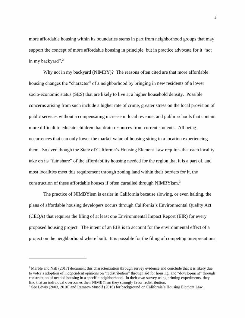
more affordable housing within its boundaries stems in part from neighborhood groups that may

support the concept of more affordable housing in principle, but in practice advocate for it “not

in my backyard”.2

Why not in my backyard (NIMBY)? The reasons often cited are that more affordable

housing changes the “character” of a neighborhood by bringing in new residents of a lower

socio-economic status (SES) that are likely to live at a higher household density. Possible

concerns arising from such include a higher rate of crime, greater stress on the local provision of

public services without a compensating increase in local revenue, and public schools that contain

more difficult to educate children that drain resources from current students. All being

occurrences that can only lower the market value of housing siting in a location experiencing

them. So even though the State of California’s Housing Element Law requires that each locality

take on its “fair share” of the affordability housing needed for the region that it is a part of, and

most localities meet this requirement through zoning land within their borders for it, the

construction of these affordable houses if often curtailed through NIMBYism.3

The practice of NIMBYism is easier in California because slowing, or even halting, the

plans of affordable housing developers occurs through California’s Environmental Quality Act

(CEQA) that requires the filing of at least one Environmental Impact Report (EIR) for every

proposed housing project. The intent of an EIR is to account for the environmental effect of a

project on the neighborhood where built. It is possible for the filing of competing interpretations

2 Marble and Nall (2017) document this characterization through survey evidence and conclude that it is likely due

to voter’s adoption of independent opinions on “redistribution” through aid for housing, and “development” through

construction of needed housing in a specific neighborhood. In their own survey using priming experiments, they

find that an individual overcomes their NIMBYism they strongly favor redistribution. 3 See Lewis (2003, 2010) and Ramsey-Musolf (2016) for background on California’s Housing Element Law.

4

of this by the developer in favor of it, and neighborhood groups opposed to it. EIRs are thus

subject to a lengthy review process, public comment, and if opposing findings, court

interpretation. NIMBYs often take this opportunity to commission an unfavorable EIR for an

affordable housing project for the economic reason of not wanting to lower residential property

values cited earlier, but often cloaked in the language of generating congestion and changing the

character of the neighborhood.

Hernandez, Friedman, and DeHerrera (2015) analyze 600 CEQA lawsuits filed between

2010 and 2012 in California and conclude that nearly 80 percent of these cases are the result of

local groups opposed to affordable infill housing development consisting of multi-unit, high-

density housing projects. Residential NIMBYism in California, utilizing the challenge offered

through an unfavorable EIR, as allowed through CEQA, has successfully prevented affordable

housing development projects from coming to fruition. For even if the positive findings of an

affordable housing development’s EIR that satisfy California’s CEQA are ultimately valid; the

threat of a prolonged challenge to them, and the cost born by the developer if it materializes;

discourages the construction of affordable housing in the State.

To deal with the tactic of using the California Environmental Quality Act to slow the

supply of affordable housing in California, Governor Brown proposed in 2016 an “As of Right”

amendment to CEQA that would have severely restricted the capacity to challenge a developer’s

proposal to build affordable housing that met all local residential building codes. This faced

resistance on multiple fronts, including: (1) environmental groups who saw it as undermining

CEQA’s intent, (2) jurisdictions that saw it as a threat to “local control” of land use, and (3)

NIMBYs who feared the loss of a tool they found effective at keeping affordable housing out of

their neighborhoods. Governor Brown’s original proposed amendment to CEQA never made it

5

out of the Legislature. But in late 2017, a diluted version of it became law (Kimberlin, 2017).

Even so, many fear this will not do enough to curtail the effects of NIMBYism on the

construction of affordable housing in the State.

To better understand the concerns of NIMBYs regarding the proximity of affordable

housing to their own residence, we desire to measure whether the greater intensity of affordable

housing in a neighborhood reduces the selling price of homes experiencing it. But measures of

greater or less affordable housing in a neighborhood are not easy to come by. As noted above, it

is not so much that existing homeowners dislike an inexpensive home in of itself, but instead fear

the lower socio-economic status (SES) and higher household density of the residents expected to

occupy it. Understanding this, we use a hedonic regression analysis of the selling price of homes

to determine the influence of poverty (or greater percentages of people in lower income

households), low educational attainment, and greater average household size. We do this using a

late 2013 data set from Sacramento County, California on the sales price of homes and their

characteristics. We choose data from 2013 because this year represents the middle of the

American Community Service (ACS) data compiled from the five years between 2011 and 2015

of the relevant characteristics of a Census Tract. We desire to offer evidence that confirms or

denies the fears of NIMBYs regarding residential property values. It is also important to place

the magnitude of these fears in perspective.

We divide the remainder of this paper into four sections. First, we offer a brief review of

empirical studies that measure the effect of greater affordable housing, and/or the characteristics

of its residents, on the value of homes in a neighborhood. Then we offer an overview of our

hedonic regression analysis and the data used to conduct it. The next section includes the

findings of our study. We follow that with a section covering the thoughts of others on

6

NIMBYism, the policy relevance of our findings, and what these findings imply for California

and other states with affordable housing concerns that can be (at least partially) blamed on

NIMBYism. We conclude with a brief description of a possible policy intervention.

Previous Literature

Early regression studies (Nourse, 1963; and DeSalvo, 1974) of the effects of affordable/public

housing construction found no effect, or even a positive effect, on nearby property values. Guy,

Hysom, and Ruth (1985) believe this due to inadequate regression techniques, and remedied it

through a more appropriate hedonic regression analysis of the effect of distance to affordable

townhouse clusters in Fairfax County (VA). They find that a shorter distance to any of these

units lowered the selling price of a home. Lee, Culhane, and Wachter (1999) continued this line

of inquiry using Philadelphia data to test the influence of proximity to distinct types of federally

assisted housing units between 1989 and 1991 on home price. After controlling for housing

characteristics, neighborhood demographics, and neighborhood amenities, they discover that

proximity to scattered-site public housing and units rented with Section-8 vouchers exert

negative influences. Relevant to our analysis, in the Lee, Culhane, and Wachter study there was

no account for the possible endogeneity of neighborhood demographics and the presence of

federally assisted housing. Even so, they did find that a higher percentage African American,

Latino, and poverty in a neighborhood reduced home prices; while, a higher median household

income drove prices up.

Green, Malpezzi, and Seah (2002) examine the impact of the proximity of housing

subsidized through Section 42, federal low-income housing tax credits (LIHTC), on sales value

of a home. They use the hedonic regression method of only looking at repeat sales data set that

allows for the control of causal variables that are unique to a specific house. They record results

7

from regressions that include and exclude the neighborhood’s poverty rate, income levels,

marriage rate, and education levels. Using data gathered from Milwaukee (WI), Green,

Malpezzi, and Seah find that the further a residential property’s distance from Section 42

housing, the greater its rate of appreciation; however, they found no influence from affordable

housing proximity using similar data from Madison (WI). Woo, Joh, and Van Zandt (2016)

study the influence of LIHTC housing on the sales price of neighboring properties using 1996 to

2007 sales data from both Charlotte (NC) and Cleveland (OH). They find that proximity to a

LIHTC property exerts a negative (positive) effect on home sales price in Charlotte (Cleveland)

that also varies by a neighborhood’s income composition. Dillman, Horn, and Verrilli (2017)

conclude with similar findings of the production of LIHTC housing in distressed (higher

opportunity) neighborhoods exerting a positive (negative) effect on nearly home values with

many forms of impact heterogeneity found.

Nguyen (2005) provides a review of 10 “first wave” studies conducted between 1963 and

1985 on whether presence of housing affordability affects property values, and the seven “second

wave” studies conducted on the same issue between 1993 and 2001. According to her

classification, first wave studies used some form of matching methodology and often lacked the

rigor necessary to trust the findings. While second wave studies relied upon the sales price of a

home and hedonic regression methodology to try and tease out the desired influence. First wave

studies predominantly found a positive to zero influence of affordable housing on neighboring

home values. Second wave studies offered more mixed results, but she summarizes their

findings as: (1) when negative effects exist they are small, (2) characteristics of affordable

housing and neighborhood composition matter, and (3) more hedonic regression studies needed

to reach a consensus on true effects.

8

The main lesson acquired through this literature review is that previous attempts to

measure the influence of the presence of affordable housing indicate only a minimal negative

effect on neighboring property values. However, only a few studies used socio-economic

characteristics of occupant characteristics as explanatory variables. And when used, they are

often in addition to measures of the degree of affordable housing. This likely generates the

concern of endogeneity that we avoid by only including SES measures in a Census Tract that are

likely to be of greatest concern to a NIMBY, and not a measure of the amount of affordable

housing itself.

Hedonic Regression Model and Data Used

The purpose of this study is to examine the consequences of characteristics of the population that

are more likely to inhabit affordable housing, on the selling price of single-family residential

properties in the same Census Tract. To do this, we use Realtor generated Multiple Listing

Service (MLS) data from late 2013 for Sacramento County. For perspective, Figure 1 offers a

map of Sacramento County and the Census Tracts located within it. Neighborhood

characteristics come from Census Tract data collected through the American Community Survey

over the five years between 2011 and 2015 (the most recent available). The general form of the

hedonic regression model is:

Selling Pricei = f (Property Characteristicsi, Selling Characteristicsi, Neighborhood

Characteristicsi) (1),

where;

Property Characteristicsi = f (Home Square Feeti, Lot Square Feeti, Years Oldi, Garage

Spacesi, Bedroomsi, Half Bathsi, Full Bathsi, Shaker Roof Dummyi, Tile Roof

Dummyi, Slate Roof Dummyi, Metal Roof Dummyi, Wood Roof Dummyi,

Foundation Raised Dummyi, Foundation Concrete Slab Dummyi, Foundation

Concrete Raised Slab Dummyi, Two-House Dummyi, Half-Plex Dummyi, Condo

Dummyi, Pool Dummyi, Fireplacesi, Stucco Dummyi, One Story Dummyi) (2),

9

Selling Characteristicsi = f (Days on Marketi, Short Sale Dummyi, Foreclosure Dummyi,

Tenant Occupied Dummyi, HUD dummyi, HOA Dummyi, HOA Duesi, FHAA

Financing Dummyi, VA Financing Dummyi, Cash Finance Dummyi, CC&R

Dummyi, November Sold Dummyi, December Sold Dummyi) (3),

Neighborhood Characteristics = f (Household Sizei, % Education Less Than HSi,

Poverty Ratei or [% Income Less $14Ki, % Income $15K-24Ki, % Income $25K-

$34Ki, % Income $35K-$49Ki, % Income $75K-$99Ki, % Income $100-$200Ki,

% Income $200K Plusi], Set of 235 Census Block Group Dummies for

Sacramento Countyi) (4).

As well established in previous hedonic-based regression research on what determines

the selling price of a house, it is necessary to account for the characteristics of the property itself.

While it is apparent that an increase in the square feet of the home and the lot it sits on,

influences the selling price of a house, factors such as the structural characteristics of the home

and years old are also likely to matter. Furthermore, it is desirable to account for observable

characteristics of the home sale that could affect what the buyer is willing to pay for it, and/or

what the seller is willing to accept. This includes the number of days that home on the market,

how financed, whether a distressed sale, if home owner association present, and the month sold.

Controlling for the characteristics of the property, along with its selling characteristics,

allows for an accurate determination of the independent influence of the relevant neighborhood

characteristics by Census Tract contained within equation (4). Neighborhood characteristics

include the average household size, a measure of the lowest educational achievement, and

poverty rate. As an alternative to the extreme of just looking for the influence of poverty rate, a

second regression examines the influences of greater percentages of different household income

categories in the Census Tract that the house sits in. We exclude a middle category of $50K to

$74K that includes the 2013 median household income in Sacramento County.

Insert Figure 1 Here

10

To control for possible unobservable neighborhood characteristics that affect the value of

a home, it is not possible to include a set of Census Tract dummies for Sacramento County

because of perfect collinearity with the SES measures assigned by Census Tract. Instead, we

include a set of Census Block Group Dummies that do not perfectly overlap with the county’s

Census Tracts.4 Table 1 offers the descriptive statistics for all the variables in this hedonic

regression study.

Insert Table 1 Here

Using the above regression model and the data just described, we estimate regressions

with the various functional forms of linear-linear, log-linear, and log-log.5 As with previous

hedonic regression analyses of the type done here, we find the log-linear functional form most

appropriate due to it exhibiting a greater percentage of statistically significant relationships. For

the explanatory variables not initially found to exert a statistically-significant influence on the

selling price of a home, we tried adding a squared value to see if an accounting for the negative

or positive effect of a variable in the log-linear form, at an increasing or decreasing rate,

generated a statistically significant finding. Depending on the specific regression, this was the

case for Lot Size, Years Old, Bedrooms, and Homeowner Association Dues. The advantage of

using the log-linear form is that the calculated regression coefficients represent the expected

decimal percentage change in the selling price of a home given a one-unit change in the

respective explanatory variable. The regression findings are in Table 2.

Insert Table 2 here

4 Census Block Groups are divisions of Census Tracts that generally contain between 600 and 3,000 people. Each

census tract contains at least one Block Group, but larger Census Tracts can contain more than one Block Group. 5 The names of these forms first refer to whether the dependent variable is in its normal or transformed natural log

form, and second refer to whether the same done for explanatory variables where possible.

11

Multicollinearity is often an econometric issue in a regression of this type. We looked for

its presence through Variance Inflation Factors (VIFs) exhibiting a value greater than five. For

regression specifications one and two, except for VIFs calculated for explanatory variables that

included their squared values, this only occurred for the three measures of foundation. Since the

foundation measures all exerted a statistically-significant influence on selling price, such

multicollinearity is not a concern. The Breusch-Pagan / Cook-Weisberg test for

heteroskedasticity indicated its presence with greater than 99 percent certainty. As described by

Cameron and Miller (2015), we dealt with the potential bias this yields in the standard errors

calculated for regression coefficients, by using cluster-robust standard errors based on the 55 Zip

Codes in Sacramento County that the housing sale data drawn from. Cameron and Miller (2015)

suggest it best to cluster over the largest group possible, while still maintaining an “adequate”

number of groups. Thus, our choice of zip codes, as opposed to Census Block Groups or Tracts

which are smaller in geographic presence.

Regarding the hedonic regression results recorded in Table 2 for property characteristics,

there were no real surprises as compared to what found in the previous literature. A one-

thousand-foot increase in a home’s square feet raises its price by a little over 30 percent. The

equivalent finding for the lot’s square feet varies by specification. In specification one, as a

home ages, its selling price first declines and then rises. Greater full and half baths in a home

also increase its value. Though interestingly, when holding square feet of a home constant, more

bedrooms initially add value, but at a decreasing rate. This is likely because of homeowner

preference for an open floor plan. Type of roof appears to make no difference to a home’s

selling price. The presence of any of the foundation types measured here, adds about a 30

percent increase in value, relative to the base category of no foundation. While if the

12

characteristics of the house accounted for in a data point pertains to two houses on a lot instead

of one, the price is about 20 percent higher. If these characteristics apply to one-story home,

instead of any other alternative, the home sells for about 8 to 9 percent more. A half-plex or

condominium, with the same characteristics, respectively gets about 15 and 37 percent less on

the market. The presence of a pool adds slight value (about 3 percent), while each fireplace

yields about a 6.5 percent increase in a home’s selling price.

Turning to the circumstances that a home sold under, the longer on the market, the less it

probably sells for. Though this was only the case in specification one that recorded about a 10

percent decrease in price after being on the market for one thousand days. A distressed home

sale, not surprisingly, reduces its resale value. Respectively, a short sale home, one in

foreclosure (Real Estate Owned), or a HUD sale (previously financed under an FHA loan, but

foreclosed upon), respectively sold for -16.2 percent, -9.5 percent, and -15.6 percent less than a

non-distressed home sale. As compared to conventional financing, a home purchased with cash

sold for about 13 percent less, while only in specification one did a home financed with an

FHAA loan sell for more. A home falling under a home owner association agreement (HOA)

sold for between 14 and 15 percent less than one without, but this tempered by the amount of

activity in the HOA (as measured by dues) exerting a positive effect on sale value at a decreasing

rate. While only in specification two did a home sold in December of 2013 fetch more than one

sold in October of the same year.

Of primary interest are the regression results recorded under Neighborhood

Characteristics in Table 2. Recall that these measure characteristics within the Census Tract of a

sold home that are expected to change if more affordable housing built there (and to be of

concern to NIMBYs). For instance, if the average household size rises by 0.53 persons (or a

13

one-standard deviation increase from the average household size of 2.84 recorded in Table 1),

the expectation is that the sales price of a home decreases by about -8.1 percent (0.53 x -0.153)

using the result in specification one (accounting only for poverty rate), and decrease by around -

11.1 percent (0.53 x -0.210) if using the result in specification two (accounting for all household

income groups). Furthermore, if the percentage of residents over age 25 with less than a high

school diploma rises by 10.16 percentage points (or one standard deviation from the mean of

13.39 recorded in Table 2), specification one indicates an expected decline in home sales value

of around -8.9 percent (10.16 x -0.00873). While specification two yields the smaller decline of

nearly -4.0 percent (10.16 x -0.00394).

The above simulations are for changes in household characteristics expected to rise if

more affordable housing built in a Census Tract. A more direct account of these expected effects

is to simulate a change in either poverty rate (as measured in specification one), or various

household income classes different than the one that contains the median home value in

Sacramento County (as measured in specification two). The poverty rate across Sacramento’s

309 Census Tracts used here varies widely from none, to just over half the population.

Specification one indicates that a one percentage point in a Census Tract’s poverty rate results in

about a -0.72 percent reduction in the sales price of a home within it. While a 10.87 percentage

point increase in a Census Tract’s poverty rate (or a one standard deviation change) results in

around an expected -7.8 percentage decrease in a home’s sales price within that Census Tract.

Hedonic regression specification two in Table 1, takes the alternative approach of

excluding the Census Tract’s poverty rate, and instead looks at the influences of percentage of

population living in the Census collected categories of household income relative to the collected

category ($50K to $74K) that includes the 2013 median household income in Sacramento

14

County of $52,980.6 This yields clear evidence that replacing a Sacramento County median

income household with a lower (higher) income household in a Census Tract, decrease

(increases) the market value of a home sold in that Census Tract. If one-percentage point of the

category containing median income households replaced with a one-percentage point increase in

household income categories of less than $14K, or $14K to $24K; the sales price falls by about a

half percent. Alternatively, if one-percentage point of the category containing median income

households replaced with a one-percentage point increase in household income category $100K

to $200K, the sales price increases by about 0.4 percent. If this decrease in median income

household category is the result of an equivalent one-percentage point increase in the highest

income households of $200K plus, the sales price of a home in the Census Tract where it

occurred rises by about 1.4 percent.

Perhaps it easier to understand these predicted changes in the selling price of a home

when put in dollar values. We do this in Table 3 for the expected change in the value of

Sacramento County’s median value home sales price in this 2013 data set of $240,000, by

simulating a one standard deviation change in the respective variables listed in the table’s first

column.

Insert Table 3 Here

Table 3 offers the expected magnitude of the dollar changes predicted by the hedonic

regression results recorded in Table 2. Recall that specification one only accounts for a rise in

the Census Tract’s poverty rate, while specification two accounts for the possibility of changes in

different household income categories. Also, note that these values can be cumulative. If a

6 See https://fred.stlouisfed.org/series/MHICA06067A052NCEN .

15

Census Tract experiences one standard deviation changes in the person size of its average

household, the percentage of its population less than high school educated, and poverty rate; the

expected decline in the $240,000 median home sales price would be -$58,188, or about a 25

percent decline.

Relevant from Table 3 is the positive influences of sales price of a home when the

household income category of $50K to $74K declines, and replaced by the higher-end

categories. The regression findings forecast that raising the $100K to $200K ($200K Plus)

category by its respective standard deviation across all Sacramento County in a typical Census

Tract, raises the $240,000 median home sales prices by $12,586 ($16,440). This represents

percentage increases of 5.2 (6.9) percent. Thus, it should not be a surprise that a homeowner is

resistant to bringing in housing affordable to those at the lowest end of the income distribution,

and likely to be much more favorable to bringing in those at the highest ends.

Conclusion

The primary intent of this study is to examine the effects of increased housing size, lower

educational achievement, and lower household income level (characteristics expected to increase

if greater affordable housing) in a Census Tract in an urban California County on the selling

price of a house within the tract. We believe that this study offers important findings relevant to

the policy debate occurring in California, and other parts of the United States, regarding how to

best address housing affordability. For as Rohne (2017) describes, many consider the lack of

housing affordability in the United States a “crisis” that extends well beyond California. In the

remainder of this concluding section, we discuss the important findings from this study, explain

the policy lessons learned from the results, and offer a response to the policy questions raised in

the introduction.

16

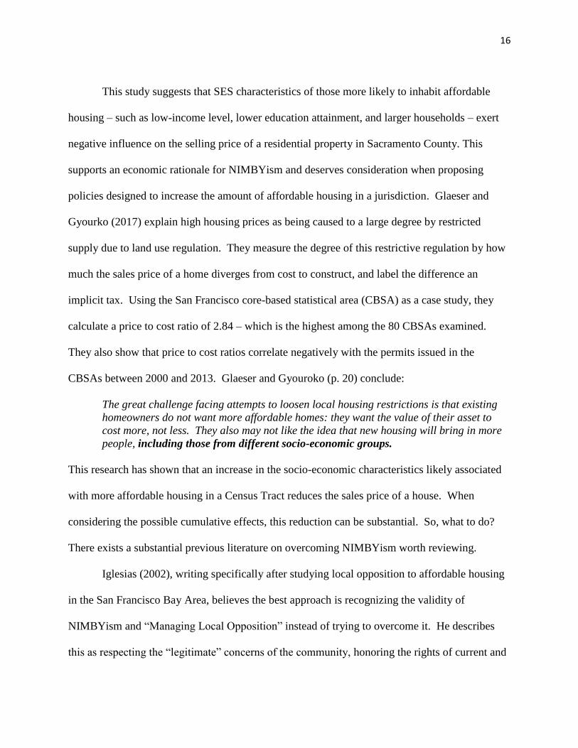
This study suggests that SES characteristics of those more likely to inhabit affordable

housing – such as low-income level, lower education attainment, and larger households – exert

negative influence on the selling price of a residential property in Sacramento County. This

supports an economic rationale for NIMBYism and deserves consideration when proposing

policies designed to increase the amount of affordable housing in a jurisdiction. Glaeser and

Gyourko (2017) explain high housing prices as being caused to a large degree by restricted

supply due to land use regulation. They measure the degree of this restrictive regulation by how

much the sales price of a home diverges from cost to construct, and label the difference an

implicit tax. Using the San Francisco core-based statistical area (CBSA) as a case study, they

calculate a price to cost ratio of 2.84 – which is the highest among the 80 CBSAs examined.

They also show that price to cost ratios correlate negatively with the permits issued in the

CBSAs between 2000 and 2013. Glaeser and Gyouroko (p. 20) conclude:

The great challenge facing attempts to loosen local housing restrictions is that existing

homeowners do not want more affordable homes: they want the value of their asset to

cost more, not less. They also may not like the idea that new housing will bring in more

people, including those from different socio-economic groups.

This research has shown that an increase in the socio-economic characteristics likely associated

with more affordable housing in a Census Tract reduces the sales price of a house. When

considering the possible cumulative effects, this reduction can be substantial. So, what to do?

There exists a substantial previous literature on overcoming NIMBYism worth reviewing.

Iglesias (2002), writing specifically after studying local opposition to affordable housing

in the San Francisco Bay Area, believes the best approach is recognizing the validity of

NIMBYism and “Managing Local Opposition” instead of trying to overcome it. He describes

this as respecting the “legitimate” concerns of the community, honoring the rights of current and

17

prospective residents, and advancing the prospects for future affordable housing. Scally and

Tighe (2015) note that it is particularly difficult to achieve equity and fairness in housing

opportunities when NIMBYism prevails in “democratic” planning processes that override these

considerations in favor of the self-interest of current residents. After surveying the previous

planning literature on locally unwanted land uses (LULUs) that drive NIMBYism, Schively

(2007) offers five mechanisms to overcome opposition: risk communication, consensus building,

empowerment, institutions, and compensation. Of interest here is her suggestion of an auction-

based mechanism for minimizing the compensation often needed to voluntarily site a necessary

LULU. But as she also notes, a consideration of using compensation is rare due to the politics of

placing equity (morality) at the forefront, which greatly diminishes the consideration of

monetary efficiency (incentives).

Hermansson (2007), writing on the ethics of LULU conflicts, questions the prevailing

attitude that NIMBYism is egotistic and irrational. Such a judgement rests on the questionable

assumption of weighting the benefits against the costs of a LULU to all impacted by it, and

instead not giving greater weight to those more directly impacted by it. Consider the scenario

she posits where a jurisdiction has zoned vacant property next to a homeowner as the site of an

“affordable housing” subdivision that will reduce the homeowner’s sales value. The homeowner

believes more affordable housing is good for society, but raises opposition to it being near her

own property. A label applied by some to individuals expressing such NIMBYism is “morally

bankrupt”. But as Hermansson points out, consider someone who declines to participate in a

medical experiment whose findings benefit society, but put the patient’s health at risk. Society,

in general, does not consider the lack of participation in such an experiment as morally lacking.

Instead, society takes the position that only volunteers should participate, and in some instances,

18

volunteers are entitled to some form of compensation for the costs imposed upon them for

participation.

To the best of our knowledge, jurisdictions in the United States rarely use compensation

to overcome NIMBY objections to greater affordable housing. Weisberg (2007) describes New

York City’s “fair-share” approach to the siting of affordable housing as involving four steps: (1)

an agreement that status quo unacceptable. (2) a participatory and open process to all

stakeholders that admits past mistakes, (3) an overall goal of geographic fairness, and (4) the

necessity keeping multiple options open. Within this approach, New York City has recognized

the potential cost to a neighborhood of locating more affordable housing there and sometimes

provides non-monetary compensation in the form of neighborhood improvements and/or tax

reductions. California has chosen to instead employ a set of “Anti-NIMBY Tools” (Rawson,

2006) centered around its statewide Housing Element Law that every jurisdiction must plan/zone

for its fair share of affordable housing necessary for the region it is part of. Though, as noted

earlier, the achievement of this affordable housing element is difficult due to local NIMBYism

and the California Environmental Quality Act (CEQA) that permits the slowdown/stoppage of its

construction if “environmental” concerns raised.

Thus, California has taken the tact of increasing laws and subsidies to encourage

affordable housing. The most recent of these occurring in a flurry of new legislation passed in

the fall of 2017. As described by Kimberlin (2017), these include: (1) a streamlined local review

process for some proposed affordable housing projects (Senate Bill [SB] 35), (2) creation of

Workforce Housing Opportunity Zones and Housing Sustainability Districts designated for

expedited development (SB 540 and Assembly Bill [AB] 73), (3) requirement that housing

element satisfaction only allowed if land has “realistic” chance of affordable development (AB

19

1397), continuous update of housing elements (SB 166), requirement for expanded analysis of

constraints on development (AB 879), and further review of housing element satisfaction with

“possibility” of reporting violations to State Attorney General (AB 72); and (4) increase burden

proof to reject housing development based on CEQA (SB 167) and requires the court to give

greater deference to housing developers in CEQA decisions (AB 1515). Even so, most do not

think that these legislative tweaks are enough to overcome California’s shortage of affordable

housing (LAO, 2016b).

Perhaps it is time for California to consider the possibility of compensation. Wassmer

(2005) earlier broached this subject by suggesting the allowance for jurisdictions most adverse to

building their state-mandated portion of regional affordable housing, compensating another

jurisdiction for doing it instead. Given that California has since embraced the market practice of

“cap-and-trade” as the preferred method of achieving its ambitious greenhouse gas (GHG)

emission goals, why not consider a version of this to overcome the pervasive NIMBYism that

exists in the siting of affordable housing? The analogy to a desired one-third statewide reduction

in GHGs, being the desire within a region that every jurisdiction satisfy its Housing Element

requirement of one-third of its housing becoming affordable to low-income residents in the

region. Under cap-and-trade for GHG reduction, the realization is explicit that it is not efficient

to require every GHG generator in the state to adhere to a one-third cut. Instead, what occurs is

the imposition of a mandate on each GHG generator to cut its emissions by one third by a certain

date in the future. Those generators not wishing to meet the mandate can buy the right to emit

more from another emitter, who would then need to emit even less. Economists recognize this as

a more efficient way of reaching the same overall goal.

20

As applied to achieving a housing affordability goal in a region, consider a jurisdiction

seeking to satisfy its one-third affordable housing element, but facing extreme resistance from

NIMBYs saying that it imposes too high a cost to do so. Under a cap-and-trade scheme, the

local policymaker could approach another jurisdiction in the region and asks how much

compensation they would need to take on an additional amount of affordable housing. Those

expecting a greater drop in home value due to affordable housing, would pay those jurisdictions

expecting to experience less. And the payment could then compensate the homeowners who

subsequently had the affordable housing placed in their backyard. A market transaction, that if it

occurs, leaves everyone better off.

Of course, cries of inequity are likely to arise because social justice norms stipulate that

every jurisdiction take on its fair share of the region’s affordable housing. Accordingly, a

compromise could be the allowance for only trading away a limited percentage (say half) of a

jurisdiction’s affordable housing element. A further equity-based safeguard could be that trade

can only occur among jurisdictions in a region if the trading jurisdictions exhibit a similar SES

profile, and are of similar distance to major employment centers. Furthermore, such a cap-and-

trade scheme would only work if also accompanied with a stepped-up increase of enforcement at

the state level of the affordable housing element for each jurisdiction. Resistance to this

increased enforcement – which is now prevalent in California under the mantra of “local control”

– should be less if cap-and-trade allowed. Jurisdictions, and the politicians that represent them,

have a market-based alternative to accepting further affordable housing that is under their local

control. Though it will cost their constituents dollars to reduce the amount of affordable housing

built in a jurisdiction, the affordable housing is built elsewhere in the region, and the jurisdiction

taking on this additional amount of affordable housing are remunerated to do so. And as shown

21

in this analysis, jurisdictions taking on more than their fair share of affordable housing are right

to ask for payment to do so.

References

Albright L., Derickson, E. S., & Massey, D. S. (2013). Do Affordable Housing Projects

Harm Suburban Communities? Crime, Property Values, and Taxes in Mount Laurel, NJ. City

and Community, 12(2), 89-112.

Bair, E., & Fitzgerald, J. M. (2005). Hedonic Estimation and Policy Significance of the

Impact of HOPE VI on Neighborhood Property Values. Review of Policy Research, 22(6), 771-

786.

California Housing Forum. (2016). 2016 California Housing Forum Key Findings

Report. Retrieved 1/7/2018 from https://caanet.org/app/uploads/2016/12/CA-Housing-Forum-

Key-Findings-Report_FINAL.pdf.

Cameron, C. & Douglas M. (2015). A Practitioner’s Guide to Cluster-Robust Inference.

Journal of Human Resources, 50(2), 317-372.

Collins, J. (2017, May 1). Housing Crisis’ Tops State’s Legislative Agenda This Year. The

Orange County Register. Retrieved 1/7/2018 from http://www.ocregister.com/2017/05/01/housing-

crisis-tops-states-legislative-agenda-this-year/.

DeSalvo, J.S. (1974). Neighborhood Upgrading Effects of Middle-Income Housing

Projects in New York City. Journal of Urban Economics, 1(3), 269-277.

Dillman, K., Horn, K., & Verrilli, A. (2017). The What, Where, and When of Place-

Based Housing Policy’s Neighborhood Effects, Housing Policy Debate, 27(22), 282-305.

Dillon, L. (2017, January 3). California's Housing Affordability Problems 'As Bad as

They've Ever Been In The State's History,' Housing Director Says. The Los Angeles Times.

Retrieved 1/7/2018 from http://www.latimes.com/politics/essential/la-pol-ca-essential-politics-

updates-california-housing-affordability-1483490282-htmlstory.html.

Galster, G. C., Cutsinger J. M., & Malega R. (2006). The Social Cost of Concentrated

Poverty: Externalities to Neighboring Households and Poverty Owners and the Dynamics of

Decline. Joint Center for Housing Studies of Harvard University. Retrieved 1/7/2018 from

http://www.jchs.harvard.edu/research/publications/social-costs-concentrated-poverty-

externalities-neighboring-households-and.

Glaeser, E., & Gyourko, J. (2017). The Economic Implication of Housing Supply.

National Bureau of Economic Research. Working Paper #w23833. Retrieved 1/7/2018 from

https://papers.ssrn.com/sol3/papers.cfm?abstract_id=3038661.

22

Green, R. K., Malpezzi, S., & Seah, K. Y. (2002). Low Income Housing Tax Credit

Housing Developments and Property Values. The Center for Urban Land Economics Research.

The University of Wisconsin. Retrieved 1/7/2018 from http://medinamn.us/wp-

content/uploads/2014/04/Low-Income-Housing-Tax-Credit-Housing-Developments-and-

Property-Values-UW-Study.pdf.

Guy, D. C., Hysom J. L., & Ruth, S.R. (1985). The Effects of Subsidized Housing on

Values of Adjacent Housing. Real Estate Economics 13(4), 378-387.

Harkness, J. & Newman, S. J. (2005). Housing Affordability and Children’s Well bEing:

Evidence from the National Survey of American Families, Housing Policy Debate, 16(2), 223-

255.

Hermansson, H. (2007). The Ethics of NIMBY Conflicts. Ethics Theory and Moral

Practice, 10(1), 23-34.

Hernandez, J., Friedman, D., DeHerrera, S. (2015). In the Name of Environment. How

Litigation Abuse Under the California Environmental Quality Act Undermines California’s

Environmental, Social Equity and Economic Priorities – and Proposed Reforms to Protect the

Environment from CEQA Litigation Abuse. Law Firm of Harold and Knight. Retrieved 1/7/2018

from http://issuu.com/hollandknight/docs/ceqa_litigation_abuseissuu?e=16627326/14197714.

Iglesias, T. (2002). Managing Local Opposition to Affordable Housing: A New Approach

to NIMBY. Journal of Affordable Housing & Community Development Law,12(1), 78-122.

Kimberlin, S. (2017). Understanding the Recently Enacted 2017 State Legislative

Housing Package. California Budget and Policy Center. Retrieved 1/7/2018 from

http://calbudgetcenter.org/blog/understanding-recently-enacted-2017-state-legislative-housing-

package/.

Lee, C., Culhane, D. P., & Wachter, S. M. (1999). The Differential Impact of Federally

Assisted Housing Programs on Nearby Property Values: A Philadelphia Case Study. Housing

Policy Debate 10(2), 75-93.

Lewis, P. (2003). California’s Housing Element Law: The Issue of Local

Noncompliance. Public Policy Institute of California. Retrieved 1/7/2018 from

http://www.ppic.org/content/pubs/report/R_203PLR.pdf.

Lewis, P. (2005). Can State Review of Local Planning Increase Housing Production?,

Housing Policy Debate, 16(2), 173-200.

Marble, W. & Nall, C. (2017). Beyond “NIMBYism”: Why American’s Support

Affordable Housing, But Oppose Local Housing Development, Working Paper, Department of

23

Political Science, Stanford University. Retrieved 1/72018 from

http://www.nallresearch.com/research.html.

Nguyen, M. T. (2005). Does Affordable Housing Detrimentally Affect Property Values?

A Review of the Literature. Journal of Planning Literature, 20(1), 15-26.

Nourse, H. O. (1963). The Effects of Public Housing on Property Values in St. Louis.

Land Economics 39(4), 433-441.

Pendall, R. (1999). Opposition to Housing: NIMBY and Beyond. Urban Affairs Review.

35(1).

Ramsey-Musolf, D. (2016). Evaluating California’s Housing Element Law, Housing

Equity, and Housing Production (1990–2007). Journal of Housing Policy Debate, 26(3), 488-

516.

Rawson, M. (2006). California Affordable Housing Law Project: Anti-NIMBY Tools.

California Department of Housing and Community Development. California Housing Law

Project. Retrieved 1/7/2018 from http://www.housingadvocates.org/docs/antinimbytools.pdf.

Rohe, W. (2017). Tackling the Housing Affordability Crisis, Housing Policy Debate,

27(3), 490-494.

Scally C.P., & Tighe, R.J. (2015). Democracy in Action?: NIMBY as Impediment to

Equitable Affordable Housing Siting. Journal of Housing Studies, 30(5), 749-769.

Schively, C. (2007). Understanding the NIMBY and LULU Phenomena: Reassessing Our

Knowledge Base and Informing Future Research. Journal of Planning Literature, 21(3), 255-

266.

Taylor, M. (2016a). Considering Changes to Streamline Local Housing Approvals.

California Office of Legislative Analyst, May 18. Retrieved 1/7/2018, from

http://www.lao.ca.gov/reports/2016/3470/Streamline-Local-Housing-Approvals.pdf.

Taylor, M. (2016b). Perspectives on Helping Low-Income Californians Afford Housing.

California Office of Legislative Analyst, February 9. Retrieved 1/7/2018 from

http://www.lao.ca.gov/Reports/2016/3345/Low-Income-Housing-020816.pdf.

Wassmer, R. (2005). An Economic View of the Causes as Well as the Costs and Some of

the Benefits of Urban Spatial Segregation. In D. Varady (Ed.), Desegregating the City: Ghettos,

Enclaves, and Inequality (pp.158-175). Albany NY: State University of New York Press.

Weisberg, B. (2007). One City’s Approach to NIMBY How New York City Developed a

Fair Share Siting Process. Journal of the American Planning Association, 59(2), 93-97.

24

Woo, A., Joh, K. & Zandt, S. V. (2015). Unpacking the Impacts of the Low-Income

Housing Tax Credit Programs on Nearby Property Values. Sage Urban Studies, 53(12), 2488-

2510.

25

Figure 1: Map of 2010 Census Tracts in Sacramento County, CA

26

Table 1: Descriptive Statistics

(4,101 Observations)

Variable Mean Std. Dev. Minimum Maximum

Dependent Variable

Selling Price 265,315 154,065 27,500 2,795,000 Property

Characteristics

Home Square Feet 1,647.06 670.73 320 7537 Lot Square Feet 201,694.70 7,167,885.07 0 2.97e+08 Years Old 35.18 21.78 0 123 Garage Spaces 1.80 0.88 0 10 Bedrooms 3.29 0.88 1 9 Full Baths 1.99 0.64 1 7 Half Baths 0.21 0.41 0 3 Shaker Roof Dummy 0.05 0.21 0 1 Tile Roof Dummy 0.30 0.46 0 1 Slate Roof Dummy 0.002 0.04 0 1 Metal Roof Dummy 0.008 0.09 0 1 Wood Roof Dummy 0.015 0.12 0 1 Foundation Raised

Dummy

0.26 0.44 0 1 Found Concrete Slab

Dummy DummyDummy

0.70 0.46 0 1 Fo Conc Raised Slab

Dummy

0.04 0.20 0 1 Two-House Dummy 0.008 0.08 0 1 Half-Plex Dummy 0.02 0.14 0 1 Condo Dummy 0.07 0.26 0 1 Pool Dummy 0.22 0.41 0 1 Fireplaces 0.83 0.54 0 4 Stucco Dummy 0.43 0.50 0 1 One-Story Dummy 0.71 0.45 0 1 Selling Characteristics

Days on Market 84.62 70.54 4 901 Short Sale Dummy 0.12 0.32 0 1 Foreclosure Dummy 0.06 0.23 0 1 Tenant Occupied Dummy 0.11 0.31 0 1 HUD Dummy 0.02 0.15 0 1 HOA Dummy 0.19 0.40 0 1 HOA Annual Dues 35.96 123.80 0 5,500 FHAA Financing

Dummy

0.21 0.41 0 1 VA Financing Dummy 0.05 0.22 0 1 Cash Financing Dummy 0.23 0.42 0 1 CC&R Dummy 0.85 0.36 0 1 November Sold Dummy 0.30 0.46 0 1 December Sold Dummy 0.33 0.47 0 1 Neighborhood

Characteristics

Average Household Size 2.84 0.53 1.3 4.21 % Education Less Than

HS School Grad

13.39 10.16 0 51.70 Poverty Rate 15.97 10.87 0 59.40 % Income Less Than

$14k

10.61 7.58 0 43.4

27

% Income $15K-$24K 9.07 5.50 0 35.9 % Income $25K-$34K 9.34 4.69 0 23.8 % Income $35K-$49K 13.12 5.60 1.1 29.6 % Income $75-$99K 13.67 5.48 1 30.1 % Income $100K-$200K 21.21 11.70 1.5 59.3 % Income $200K Plus 4.96 4.93 0 27.0

Table 2: Regression Results Using Log of Selling Price as Dependent Variable^

(4,101 Observations, Clustered [on 55 Zip Codes] Robust Stand Errors Used)

Explanatory Variable# Specification One~ Specification Two

Property Characteristics

Home Square Feet (1,000s) 0.347***

0.304***

Lot Square Feet (1,000s) 0.00000401** -0.0000000102 Lot Square Feet Squared -1.43e-11** - Years Old -0.0116*** -0.0103*** Years Old Squared 0.000116*** 0.000103*** Garage Spaces 0.0394*** 0.0391*** Bedrooms 0.214*** 0.227*** Bedrooms Squared -0.0305*** -0.0310*** Full Baths 0.0567*** 0.0615*** Half Baths 0.0465*** 0.0469*** Shaker Roof Dummy 0.0361 0.00660 Tile Roof Dummy 0.0100 -0.0119 Slate Roof Dummy 0.0350 -0.00132 Metal Roof Dummy 0.0310 -0.00484 Wood Roof Dummy+ 0.0289 0.00601 Foundation Raised Dummy 0.352*** 0.325*** Foundation Concrete Slab

Dummy

0.261*** 0.252*** Found Conc Raised Slab

Dummy++

0.297*** 0.277*** Two-House Dummy 0.201*** 0.179*** Half-Plex Dummy -0.150*** -0.151*** Condo Dummy -0.396*** -0.363*** Pool Dummy 0.0288** 0.0365** Fireplaces 0.0646*** 0.0616*** Stucco Dummy -0.000197 0.00226 One-Story Dummy 0.0920*** 0.0823*** Selling Characteristics

Days on Market -0.000103* -0.0000854 Short Sale Dummy -0.162*** -0.160*** Foreclosure Dummy -0.0947*** -0.0924*** Tenant Occupied Dummy -0.0604*** -0.0653*** HUD Dummy -0.156*** -0.142*** HOA Dummy -0.167*** -0.169*** HOA Annual Dues (1,000s) 0.514*** 0.346***

28

HOA Annual Dues Squared

(1,000s)

-0.0920*** -0.0544*** FHAA Financing Dummy 0.207** -0.0116 VA Financing Dummy -0.00650 0.00326 Cash Financing Dummy+++ -0.134*** -0.127*** CC&R Dummy 0.000368 0.00204 November Sold Dummy 0.00165 0.00199 December Sold Dummy++++ 0.0119 0.0129* Neighborhood Characteristics Average Household Size -0.153*** -0.226*** % Education Less Than HS

School Grad

-0.00873*** -0.00355* Poverty Rate -0.00715*** - % Income Less Than $14K -

-0.00496* % Income $15-$24K - -0.00470*** % Income $25-$34K - -0.00110 % Income $35-$49K - -0.000849 % Income $75-$99K - -0.000311 % Income $100-$200K - 0.00437** % Income $200K Plus+++++ - 0.0137***

R-Squared 0.848 0.865

^ Data on home selling price and characteristics drawn from all residential home sales in

Sacramento County, CA in last quarter of 2013. Neighborhood characteristics drawn from 2011-

2015 American Community Survey.

#We also include a set of 234 dummy variables representing each of the Census Block Groups in

Sacramento County for which a home sold under the period of observation. The results not

recorded here.

~Each cell contains the calculated regression coefficient which represents the expected

percentage change in home sales price (in decimal form) from a one-unit change in the

respective explanatory variable.

***Indicates statistical significance from zero in a two-tailed test at the 99% or greater

confidence level; ** 95-99 confidence level; and * 90-95 confidence level.

+Composition Roof is the excluded category. ++No Foundation is the excluded category.

+++Conventional Financing is the excluded category. ++++October Sold is the excluded

category. +++++% Income 50-74K is the excluded category.

29

Table 3: Expected Dollar Change in 2013 Market Value ($240K) Home in Sacramento

County from Given Change in Neighborhood Characteristic that May Change After

Greater Affordable Housing in Census Tract

Neighborhood Characteristic Specification One Specification Two

Average Household Size

(mean of 2.84)

rises one standard deviation of 0.5 persons

-$18,360^

-$27,120

% Education Less Than HS

(mean of 13.39)

rises one standard deviation of 10 percentage

points

-$20,952

-$8,520

Poverty Rate

(mean of 15.97)

rises one standard deviation of 11 percentage

points

-$18,876

-

% Income Less than $14K

(mean of 5.45)

Rises one standard deviation of eight percentage

points

-

-$9,024

% Income $14K to $24K

(mean of 9.07)

Rises one standard deviation of six percentage

points

-

-$6,768

% Income $100K to $200K

(mean of 21.21)

Rises one standard deviation of 12 percentage

points

-

$12,586

% Income $200K Plus

(mean of 4.96)

Rises one standard deviation of five percentage

points

-

$16,440

^Calculated as (0.5 Persons x -0.153 Regression Coefficient) x $240,000 median home value.