UNIVERSITY OF VAASA FACULTY OF BUSINESS STUDIES

DEPARTMENT OF ACCOUNTING AND FINANCE

Vilhelm Bengs

DOES THE ‘FITNESS’ OF A FIRM AFFECT ITS INVESTMENT BEHAVIOR? EVIDENCE FROM GERMAN MARKET

Master’s thesis in Accounting and Finance

VAASA 2016

brought to you by COREView metadata, citation and similar papers at core.ac.uk

provided by Osuva

1

TABLE OF CONTENTS Page 1. INTRODUCTION 9 2. LITERATURE REVIEW 12

2.1. The neoclassical q-theory of investment 12

2.2. Imperfect markets approach 17

2.3. The evolutionary approach 22 3. THEORETICAL BACKGROUND 28

3.1. A frictionless economy 28

3.2. Market imperfections and the theory of investment 32

3.2.1. Heterogeneous capital and information asymmetries 32

3.2.2. Agency problems in the theory of investment 37

3.3 The Evolutionary theory 39 4. DATA AND METHODOLOGY 43

4.1. Data 43

4.2. Methodology 50

5. EMPIRICAL RESULTS 53

5.1. Empirical results of the full and subsamples 53

5.2 Robustness of the results 59

2

3

6. CONCLUSION 61 REFERENCES 63 APPENDIX 68

4

5

LIST OF FIGURES AND TABLES

FIGURES Figure 1. The hierarchy of finance model with no debt finance. Figure 2. The hierarchy of finance model with debt finance. Figure 3. There exists an interest rate which maximizes the expected return to the bank. Figure 4. Determination of the market equilibrium. Figure 5. Relative competitive advantage. Figure 6. Different circumstances in the economy. Figure 7. Subsample classification. Figure 8. CDAX index. TABLES Table 1. Extracted variables. Table 2. Descriptive statistics of key variables. Table 3. Descriptive statistics of unmodified key variables. Table 4. Descriptive statistics of total assets and debt to equity ratios for full and subsamples. Table 5. Industry classification and average number of observations in each industry and variable. Table 6. Empirical results of the full sample. Table 7. Empirical results of subsamples with capital expenditures as the dependent variable. Table 8. Empirical results of subsamples with R&D as the dependent variable. Table 9. Empirical results of the full sample, without industry adjusting.

6

7

UNIVERSITY OF VAASA Faculty of Business Studies Author: Anders Vilhelm Bengs

Topic of the thesis: Does the ‘fitness’ of a firm affect its investment

behavior? Evidence from German market

Name of the supervisor: Jussi Nikkinen Degree: Master of Science in Economics and Business

Administration

Department: Department of Accounting and Finance

Major Subject: Finance

Year of Entering the University: 2010

Year of Completing the Thesis: 2016 Pages: 69

ABSTRACT

This thesis examines the evolutionary firm-level investment theory. The theory states that firm behavior is not driven by profit maximization in an equilibrium economy. Rather, the economy is a dynamic environment, where firms strive to survive and grow. Firms which encompass vital skills will grow and overtake larger market shares, while weaker firms deteriorate and, eventually, exit the market.

The purpose of this study is to empirically examine if ‘fitter’ firms invest more compared to ‘weaker’ firms. Three measures of firm ‘fitness’ is used, industry adjusted cash flow, return on investment and return on assets and two measures of investment, capital expenditures and research & development expenses. The data covers eleven years of observations spanning from 2004 to 2014 and consists of listed German firms. The full sample is divided into three subsamples: Pre-crisis, crisis and post-crisis period in order to examine the effects of a business cycle. The most reliable results are obtained from the full sample and by using capital expenditures as the dependent variable. The results in this sample are convincing; firms which belong to the upper quartile, measured by the three proxies of fitness, seem to invest more compared to firms belonging to the lowest quartile.

The results of the full and subsamples regressed on R&D expenditures are peculiar. These findings are contradictory to findings, where capital expenditures is used as the dependent variable. A plausible explanation to this phenomenon may rest on insufficient observations in regards to reliable results. Thus, a knowledge gap for future research is left open, both for examining the effects of firm-level R&D behavior and, especially, how the evolutionary theory fits small firms.

KEYWORDS: Evolutionary theory, firm-level investment, financial constraints, capital heterogeneity.

8

9

1. INTRODUCTION

Allocation of resources to productive firms is an essential process in any market-driven economy. Thus, a solid understanding of investment from a microeconomic perspective is important. During the 1960’s the first groundbreaking firm-level investment theories were introduced by Jorgenson 1963 and Tobin 1969. According to these theories, firm-level investment is linked to the aggregated demand of capital in the economy, which on the other hand is determined by the market conditions in the economy. The Cobb-Douglas production function was the underlying theory on which firm-level investment theories were built; Hayashi (1982) combined Tobin’s (1969) q-theory and the neoclassical production function theory into one flawless mathematical formula, defining the optimal firm-level rate of investment. However, Hayashi’s (1982) model, and Tobin’s q-theory assumes perfect market conditions, which rarely, if never hold in the real world of business. In the late 1980’s the availability of firm-level data increased and the theoretical models could be tested empirically. As it turned out, the q-theory, failed in many empirical tests (Audretsch & Elston 2002; Fazzari, Hubbard & Petersen 1988a; Gilchrist & Himmelberg 1995). This resulted in an ongoing debate among academics whether the q-theory is only valid in a frictionless economy or if the actual problem was in measuring q correctly (Barnett & Sakellaris 1998: Erickson & Whited 2000: Gomes 2001)? The theory states that the q-value (market value/book value) should be equal to one (Coad 2010; Yoshikawa 1980). In the absence of information asymmetries investors are able to assess each firms net present value and, therefore, correctly price all shares. Hence, if the q-value is greater than one, it means that these firms have a high demand for their products or services. Thus, if the q-value exceeds one a firm should increase its production capacity, which requires capital. Eventually, q will be driven down to one, where the marginal productivity of capital equals the marginal cost of capital. On the other hand, if the q-value is below one, it signals inefficient usage of resources. Within those circumstances a firm would increase its profits by decreasing its production capacity, until the marginal productivity of capital equals the marginal cost of capital. However, these conclusions hold only if information is equally available to all actors, if markets are competitive, capital is homogenous and firms act rationally to maximize the value of shareholders.

10

Generally speaking, no frictions should exist in an economy, which could affect for some individuals, firms or institutions the price of input factors in the production function favorably or discriminatingly. (Coad 2010; Hayashi 1982; Tobin 1969; Yoshikawa 1980) It can be argued that in the presence of frictions, such as information asymmetries and capital heterogeneity in an economy, inevitably the q-theory fails to explain investment behavior due to violations of the underlying assumptions. Fazzari et al. (1988a) demonstrate that current financial performance, measured by cash flow, is significant in explaining firm-level investment. Their findings set in motion a vast amount of research, modifying the q-model and examining how financial constraints affect firm-level investment. In addition to the q-theory of investment and the imperfect market theory, an evolutionary approach has been developed (Coad 2010). The basic principle of the evolutionary approach is that firms are not able to act rationally in an uncertain world and even less capable of forecasting accurately future profits (Alchian 1950). In addition, an economy can never reach a state of equilibrium due to frictions. Therefore, an economy is under constant change caused by shocks, e.g. in prices or regulation. In comparison to the q-theory, the evolutionary approach accepts certain imperfections in the system. Hence, firms which are able to adapt have better chances of staying competitive. The fundamental idea in the evolutionary approach is established on Ronald Fisher’s (1930) findings in population genetics, according to which the fittest will survive. For example, Coad (2010) has conceptualized Fiseher’s (1930) theory into a firm-level investment theory. Succinctly described, a firm is able to invest and grow if it can maintain a level of ‘fitness’ greater than an average firm. A proxy of fitness can be measured as higher cash flow, return on investment or return on assets compared to industry peers. The purpose of this thesis is to empirically test the evolutionary theory in the German economy. More specifically, whether firms having higher industry adjusted cash flow, return on investment and return on assets show a positive impact on capital expenditures and research & development expenses. Thus, the following hypothesis is formulated and tested.

H1: fitter firms invest more compared to weaker firms.

11

The theoretical framework for the hypothesis is based on the idea that the economy is a dynamic environment, where some firms are better coped in recognizing profitable investment opportunities than others. These firms encompass unique skills, which have enhanced over time. Thus, firms strive to constantly improve their performance in order to maintain competitive, therefore, the ones that succeed will have a higher level of fitness. Some firms might be able to improve, however, not quicker or better than their competitors and, consequently, these firms are weaker. (Coad 2010; Metcalfe 1994) For some reason the evolutionary theory has not received wide attention in the academic community and has not, therefore, been thoroughly examined. A lot of effort has been taken on investigating, whether financial constraints affect firm-level investment from the scope of traditional investment models, such as the q-theory, and many modifications of it; instead of questioning the applicability of the traditional approaches and their underlying assumptions. To the best of my knowledge, the evolutionary theory has not been tested on German firms. Therefore, the results of this thesis will increase our knowledge of German firm-level investment behavior and, additionally, strengthens the theoretical applicability of the evolutionary theory in this specific economy. The remainder of this thesis is structured as follows: Chapter 2 introduces previous studies regarding firm-level investment. Chapter 3 discusses the theoretical background. In chapter 4 the data and methodology are discussed and in chapter 5 the empirical results are presented. Lastly, chapter 6 concludes and suggests areas for future research.

12

2. LITERATURE REVIEW

This section introduces essential firm-level investment literature. Coad (2010) classifies the literature into three different categories: the neoclassical q-theory, an imperfect markets approach and the evolutionary theory. The focus in this chapter is on how the theoretical frameworks have been applied, while the next chapter focuses on theoretical evolution of firm-level investment approaches. A clear distinction especially between the neoclassical q-theory and the imperfect markets approach is difficult to draw. In this thesis, the literature is mainly categorized based on the methodologies which have been used; if the q-theory has been the main method it is discussed under section 2.1. Although, the traditional neoclassical q-theory assumes a frictionless economy, many papers which are categorized under section 2.1. do not. Primarily, the categorization of the sub-sections is based on whether the study concludes that the q-theory can fully (if correctly measured) explain firm-level investment. However, if the conclusion follows that current financial performance, such as cash flow, may affect investment then these papers are described under section 2.2. Imperfect markets approach. Section 3.3. discusses the evolutionary approach.

2.1. The neoclassical q-theory of investment

The neoclassical q-theory of investment is built upon research papers, such as, Jorgenson (1963), Tobin (1969) and Hayashi (1982). Jorgenson (1968) argues that a firm maximizes its profits according to the Coubb-Douglas (1928) production function. Therefore, investment will be determined by the need of the aggregated level of capital in an economy, which on the other hand is determined by the market conditions at a specific point in time. These conditions change according to price, technology, demand and alike. Tobin (1969) proves how a single ratio, called q is able to capture a firms need of capital. He further argues that capital should be related to its replacement cost. A popularized calculation of Tobin’s q is the market value of a firm divided by the book value of assets (Coad 2010). Hayashi (1982) combines the neoclassical production function theory and Tobin’s q-value and proves mathematically how the q-value can be of use in the theory of investment. According to Hayashi (1982) the modified q-value (see section 3.1) is able to

13

explain a firms optimal rate of investment. However, Hayashi’s (1982) theory assumes perfect markets. The early empirical research on investment was limited on aggregated market data, which did not allow the researchers to analyze firm-level behavior. The results on aggregated data, such as Hayashi’s (1982) empirical analysis, show strong positive serial correlation in the error term. To summarize, it has proven considerably difficult for researchers to estimate accurately q. Extensive discussion throughout decades of investment literature has argued whether poor results are due to inaccurate measures of q, estimation techniques or due to market imperfections, or perhaps a combination of both. Schaller (1990) states that the q-theory has been unsatisfactory in empirical results. He considers the reason to be a misspecification of average q. More specifically, an upward bias in adjustment costs as well as market imperfections, which violates Hayashi’s (1982) conclusion of average and marginal q. Schaller (1990: 310) concludes that q is able to explain a rather small portion of the variation in investment. Additionally, the unexplained part is often highly serially correlated. The cause for this, according to Schaller (1990) originates from the aggregated data used in previous studies. To tackle the aggregation issue he examines 188 large publicly traded firms in the United States with data spanning over a long sample period, from 1951 to 1985. By using firm level-data Schaller (1990) was able to prove that serial correlation in the error term reduced significantly. He reasons that allowing firm-level heterogeneity in adjustment costs captures the divergence among firms in a more plausible way. Moreover, Schaller (1990) identifies that imperfect competition should be accounted for, although he is not able to distinguish between financially constrained firms and imperfect competition. Besides Schaller (1990), Erickson et al. (2000) investigates the misspecification of q-theory models. They contradict Fazzari et al. (1988a), article which shows that cash flow is a significant variable explaining investment. According to Erickson et al. (2000) the reason for cash flow being significant relies on the fact that q has been previously incorrectly measured. The authors examine 737 American manufacturing firms over a four year period between 1992 and 1995. They argue that by using a generalized method of moments (GMM) in the econometric applications captures the true nature of marginal q and removes the “noise” from measurement error. Additionally, Erickson et al. (2000) demonstrate that q still remains significant even after controlling for financially constrained firms. The authors choose firm size and bond ratings to describe financial strength. Erickson et al. (2000) consider small firms being financially constrained as they are more likely to face information asymmetries compared to large firms. Firms are

14

classified as small if they belong to the lowest 33 percent on each of the four year total asset distributions. This particular method of classification yielded in 217 constrained firms. Additionally, Erickson et al. (2000) considered firms being unconstrained if they had a Standard & Poors bond rating, this type of classification returned 459 constrained firms. Based on their results Erickson et al. (2000: 1050) argues that cash flow has no place in advanced investment theory. However, they point out that q-theory is not the “last word” as, for example, learning and capital heterogeneity are important characteristics defining firm investment decisions. Gomes (2001) finds similar results as Erickson et al. (2000). He uses an unbalanced panel data containing 12 321 American firm year observations from 1978 to 1988. Furthermore, Gomes (2001) summarizes the investment decision making process for a firm into three options; Firstly a firm has to decide whether to stay operative or exit the market. This decision should be based on a simple fact; if a firms expected profitability is below the market value of its assets the rational choice would be to liquidate the firm and exit. Secondly, if a firm chooses to stay, then the decision comes down on how much should be invested and, thirdly, how should the investment be funded. However, Gomes (2001) does not clearly specify how firms should choose the optimal level of investment if they choose to stay in the market. According to Gomes (2001) financing constraints affect firm behavior. Therefore, he focuses on examining how financing constraints affect cash flow as an independent variable in a neoclassical investment model. In order to examine the explanatory power of cash flow, Gomes (2001) created an artificial equilibrium economy on which he simulated different types of investment models. His final results were based on comparison, between the artificial and empirical data sets. Gomes (2001) claims that in his empirical data set cash flow remains a significant variable explaining investment. However, he continues that the true reason for this is in fact that investment decisions are nonlinear and by applying a linear equation in efforts to explain the phenomena will lead an econometrician to falsely accept cash flow as a significant variable. Gomes (2001) concludes by using his theoretical approach that cash flow is unable to explain investment. He adds, that a fully specified q-model captures financial constraints as these constraints should be incorporated into the market price of a company and, therefore, in q.

15

Barnett et al. (1998) examines nonlinear properties of investment in relation to q. They claim that q might have varied sensitivities to investment within different regimes. These regimes are specified according to firm level q values. Barnett et al. (1998) conducts their study on an unbalanced panel consisting of 1 561 firms. They use a method proposed by Hansen (1996) which allows estimating whether an unobserved variable is above or below a threshold value. (Barnett et al. 1998) Barnett et al. (1998) finds that the nonlinear approach results in higher sensitivity of q in relation to investment compared to the traditional linear approaches. Moreover, the sensitivity of q is s-shaped. Hence, low q values tend to increase the responsiveness to investment, also intermediate values increases and high q values tend to have a flat effect in relation to investment. Contrary to what Gomes (2001) argues, Barnett et al. (1998) concludes that, when a nonlinear estimation technique is used cash flow remains a significant variable. During 1990’s, a strand of literature using the Euler equation became popular in describing the investment process. Coad (2010) concludes that the Euler equation is ultimately derived from the same principles as the q-theories. However, the benefit in the approach is in not having to measure q, which has proven to remain a difficult task (Coad 2010: 207). Whited (1992) explores the Euler equation approach to overcome one of the violations of the q-theory, namely the one that presumes capital being homogenous. He considers access to funding to be heterogeneous among different firms. Whited (1992) based his analysis on data of 325 U.S. Manufacturing firms of which 286 are from the combined Compustat file and 39 from the OTC Compustat file. The time period spans from 1975 to 1986. Whited (1992) divides the firms into constrained and unconstrained firms with three indicators: firstly, high debt to asset ratios and secondly, high interest coverage ratios. Thirdly, he considers firms not having a bond rating to be constrained, as firms having a rating are more likely to have undergone a scrutinized evaluation. Therefore, information asymmetries are more unlikely among the rated firms. Whited (1992) concludes that by including financial constraints in the Euler equation substantially improves the model. He reasons that due to information asymmetries between firms and investors, especially small constrained firms are unable to obtain external finance to a reasonable price. Moreover, Whited (1992) finds supportive

16

evidence to his theory. Firms not participating in the corporate bond market show significant evidence on financial constraints affecting investment. Galeotti, Schiantarelli & Jaramillo (1994) examine small and large Italian manufacturing firms. They investigate if Italian firms are affected by financial constraints regarding investment. Galeotti et al. (1994: 124) include 3 039 small firms in their data set and 43 large firms. Since – the q-model requires observed market values the Euler equation is used to estimate constraints on small firms and the q-model in the large firm data set. Two issues are highlighted concerning the models: the unobservable variables and the endogeneity (correlation with the error term) of the independent variables. To overcome these issues, the authors state the error term to consist of two random components: a fixed, unobservable firm-specific effect and a pure white noise disturbance. Specifically, first differentiating and a moving average with a time lag of one are used to mitigate the unobserved effect and endogeneity. (Galeotti et al. 1994) Galeotti et al. 1994 demonstrate two main findings. Large firms are insensitive to cash flow while small firms are sensitive. The authors believe that large companies are less constrained, due to the fact that information asymmetries are small between investors and managers. Concurrently, small companies are more likely to have difficulties in obtaining external financing, which is proven by a statistically significant cash flow regressor. However, Galeotti et al. (1994) add that it is not surprising for large firms to show insignificance towards cash flow. The Findings reflect a relatively stable time period 1976–1986 and additionally, the concentrated ownership structure illustrates a significant role. (Galeotti et al. 1994) Bond & Meghir (1994a) also study the effects of financial constraints on investment behavior. Similarly to Whited (1992), Bond et al. (1994a) consider capital to be heterogenous for firms. Therefore, they choose to examine 626 listed UK manufacturing firms between 1971 and 1986. Their assumption is that external funding is more expensive than internal. In order to examine the relationship between internal and external funding they divide the companies into three regimes, which describes the firms desire to invest in relation to available sources of funding. Bond et al. (1994a) argue that share prices do not always capture true fundamental value of firms. Thus, the Euler equation which does not require market value, is a better choice for estimating firm-level investment than the q-model. They use a model in which both the current and the prospective years’ investment ratio is included. This type of approach

17

allows firms to be categorized in separete regimes during different years. These regimes are constructed by measuring a firms dividend payout policy. Regime one includes firms which pay high dividens compared to their usual dividend payout ratio and do not issue new shares. Regime two includes firms that, are considered to be unconstrained. Furthermore, the regression coefficients are compared between the two regimes. The empirical results show that the two regimes behave differently. The authors conclude that the investment ratio of U.K. firms is likely to be affected by the availability of internal finance, which supports the idea of hierarchical finance.

2.2. Imperfect markets approach

Better obtainability of firm-level data from the late 1980s onwards enabled more extensive empirical examination of investment theories (Schiantarelli 1996: 70). Hence, researchers challenged the traditional q-theory view with strict assumptions of – perfect competition and homogenous capital markets, which are required for the theory to be valid. The failure of empirical research to establish the investment model proposed by Hayashi (1982) led researchers to accept that imperfect markets might affect investment behavior. Fazzari et al. (1988a) examines how cash flow affects investment behavior. Despite contrary findings, (see e.g., Erickson et al. 2000), Fazzari et al. (1988a) became a much-cited milestone in the investment literature. Fazzari et al. (1988a) use data on U.S. manufacturing firms between 1970 and 1984. They analyze from several angles cash flow’s significance in explaining investment. Their core idea is to divide firms into three classes based on dividend payout ratios. Firms with the lowest ratios are considered to be immature and face financial constraints in obtaining external finance. On the other hand, class three contains firms with high dividend payout ratios and these firms are expected to face little or no constraints. Fazzari et al. (1988a) hypothesize that due to market imperfections cash flow should add significant explanatory power into the traditional q model. Market imperfections are mainly considered to stem from asymmetric information and bankruptcy costs. The authors argue that information asymmetries between a firm and potential investors cause an extra premium on external finance. This creates capital heterogeneity, which

18

presumable is more likely for firms in class one than for firms in class three. Furthermore, a firm taking additional loan increases bankruptcy costs as fixed charges rise and investors require a higher premium for the additional risk. Investors limit the excess loan taking of firms by including covenants in the loan contracts, which might further limit firms of issuing new loans, even in the event of a lucrative investment opportunity. Additionally, Fazzari et al. (1988a) highlight taxes, agency problems and transaction costs as possible frictions in the market. Furthermore, they consider information asymmetries to be highly relevant as an additional friction factor. (Fazzari et al. 1988a) Fazzari et al. (1988a) use the traditional q-theory approach, however, including cash flow. Their findings show that cash flow is significant in all three classes. This result was somewhat contradictory to the expected result regarding class three. However, the authors point out that stock markets are volatile and do not always represent fundamental value. Also, q might include measurement errors. Therefore, to assure result robustness, Fazzari et al. (1988a) run regressions with lagged q and, additionally, regressions using first and second differentiating. After robustness analyses cash flow remained significant in all three classes. Fazzari et al. (1988a) point out that, even though, cash flow shows significance in all three classes, notable differences exist among the firms. The firms that retained approximately all of their earnings showed greater sensitivity on cash flow to investment compared to firms that paid dividends. Gilchrist et al. (1995) extends the findings of Fazzari et al. (1988a) regarding investment models and the role of cash flow in these models. Moreover, Gilchrist et al. (1995) examines whether cash flow is plausible in explaining future investment opportunities for firms or financial constraints. The authors construct what they call “Fundamental Q” and test this model against the traditional q model. Fundamental Q is a more sophisticated version of the traditional q model proposed by Hayashi (1982). It includes the same basic principles – however, also including ratios of profit to capital and sales to capital ratios. According to Hayashi (1982) marginal q is equal to modified q, which is calculated by dividing future after tax net receipts (interpreted as market value) with the value of investment goods (book value). The benefit in Gilchrist et al. (1995) model is that it does not require market value. As the net present value of future profits are considered to be captured by profit and sales. Therefore, the model is applicable for unlisted firms. Gilchrist et al. (1995) include in their fundamental Q model cash flow, and reasons that if financial constraints are present, then cash flow should show significance. On the other

19

hand, in the absence of financial constraints cash flow should be insignificant. To capture dissimilarities between firms, the authors list several proxies capturing financial constraint. The proxies are: corporate bond issuance, bond rating, dividends and size. More specifically, a firm is considered to be financially constrained if the dividend payout ratio or size falls below the 25th percentile. Gilchrist et al. (1995) obtained 470 U.S. manufacturing firms from Standard & Poors Compustat data base after deleting firms involved in mergers and acquisitions. The data spans from 1979 to 1989. Noteworthy, is the fact that an additional 42 firms were deleted due to extreme values prior the estimation period in cash flow, investment, sales and Tobin’s q. In detail, for instance Tobin’s q is set to be between 0 and 10. The authors argue that the rule is set to reduce measurement error in computing q. The error can rise from large discrepancies between market and book value of debt, and because of large amounts of intangible assets on the balance sheet (Gilchrist et al. 1995). Gilchrist et al. (1995) compare the augmented fundamental Q model and the fundamental Q model excluding cash flow. Their findings show that unconstrained firms show insignificance for cash flow as for constrained firms cash flow is significant. The results amplify findings suggested by previous studies, such as Fazzari et al. (1988a). However, a difference remains among the unconstrained firms, where Fazzari et al. also demonstrate significance of cash flow. The authors conclude that the traditional q model is an erroneous proxy for investment opportunities (Gilchrist et al. 1995: 567). Audretsch et al. (2002) examine if German firms face financial constraints. The authors point out that the German financial system is in two ways highly different compared to the Anglo-Saxon model. Firstly, the German firms rely heavily on external finance provided by the banking sector. Secondly, bank representatives are often positioned in the supervisory boards of German firms. Considering these two characteristics the authors anticipate their findings to differ from the empirical studies made on U.S. and U.K. data. Audretsch et al. (2002) use a generalized method of moments regression, where the dependent variable is investment divided by the firms capital stock. The regression includes six independent variables, which are: investment, q-ratio, cash flow, sales, size and ownership concentration. Investment, cash flow and sales are scaled by the capital stock. Additionally, all variables are lagged by one year. Therefore, previous year’s investment is anticipated to affect current year’s investment. Firm size is measured as the natural logarithm of net sales. Furthermore, ownership concentration is divided into five

20

categories, the first category representing the highest degree of ownership, where one shareholder has more than 75% percent of the outstanding shares. The fourth category represents the second highest diversity in ownership and includes firms where two or three stockholders own more than 50% of the shares. The fifth category includes all other firms, which do not belong to any other category. The sample firms are also divided into four size categories based on the total number of employees, where number one represents the smallest firms and number five the largest firms. The final sample used by Audretsch et al. (2002) consists of 100 listed firms. The time interval covers 17 years from 1970 to 1986. They conclude that cash flow is significant on 8 out of the first 11 years. After 1981 only one year is significant in cash flow and only with a 10% significance level. Audretsch et al. (2002) reasons this being due to the increased competition in the banking sector in the 1980s, which eased the availability of finance. Furthermore, q was significant on 6 of the 17 years and ownership concentration remained insignificant throughout the sample. Interestingly, medium sized firms showed higher significance on cash flow compared to small and large firms. The authors argue that these firms are financially constrained, whereas large and small companies are not. They believe it is because of the special characteristics of the financial system in Germany, where funds are specifically channeled to small firms. Large firms on the other hand are able to raise funds by issuing new shares on the stock market. Bond, Elston, Mairesse & Mulkay (2003) study the effects of financial constraints on investment in Belgium, France, Germany and the United Kingdom. The purpose of their study is to compare the three continental European countries to the more market oriented financial system in U.K. The authors use two different methods: a GMM error-correction model and an Euler equation model. These two approaches are not examined as competing, rather as complementing measurement systems. Bond et al. (2003) use a panel data set which spans from 1978 to 1989. The Belgian panel represents 361, the French 1 365, the German 228 and the U.K. sample 571 firms, respectively. Firms which had less than 100 employees in the first sample year were excluded. Additionally, only manufacturing firms were examined. The authors hypothesize that firms operating in the three European countries were expected to be less or not at all financially constraint due to the characteristics of the banking system in these countries.

21

The empirical results confirm the hypothesis. The most significant differences are found between Belgium and U.K. The Cash flow variable is insignificant among Belgian firms and strongly significant for U.K. firms in the error-correction model. Additionally, the null hypothesis that no financial constraints are present was accepted for Belgium and rejected for U.K. Investment in French and German firms were sensitive to cash flow, however, significantly less than the U.K firms. The authors conclude that their results are robust and argue that U.K. firms are significantly more constrained than the firms of the other three European countries. In addition, they point out that cash flow could reflect expectations of future profits. However, the data showed no proof that cash flow could forecast future sales growth or profitability in their econometric tests. Nevertheless, considering the length of the sample period, the authors mention that it is a possibility that their results are revealing only temporary conditions in the respective countries rather than clear differences between the financial systems. (Bond et al. 2003) Lamont (1997) designed an event study based on the 1986 oil price decline in order to establish evidence on market imperfections. The research question is formulated to answer whether investment is reduced if cash flow or collateral value falls, even though investment opportunities are unchanged or higher. Lamont (1997) defines that companies that have business operations in both the oil and nonoil industry are well suited for his study. He reasons, that investment in the nonoil segments should not show any difference in investment behavior caused by the oil shock, in the absence of information asymmetries. He argues that if market imperfections do not exist then corporate segments should operate as separate units and finance their investments based on unit level internal and or external finance. Lamont (1997) gathers data from the Compustat data base. He sorts firms based on their two-digit SIC code (13) to isolate oil-dependent firms. He defines a firm of being oil-dependent when at least 25 percent of the firms cash flow is generated by the oil and gas extraction industry. To define oil-dependent and oil independent business segments Lamont (1997) evaluates the selected firms financial reports and examines the nonexistence of positive profits correlation with oil. The data selection process yielded in 26 suitable U.S. firms with available data on 1985 and 1986. Lamont’s (1997) findings show that cash flow and collateral value shortfalls affect investment negatively. However, Lamont (1997) is unable to conclusively establish underlying factors for this. He concludes that another possible explanation beyond asymmetric information and access to external capital markets can be overinvestment.

22

During high cash flow times firms might overinvest in poorly performing business segments. When cash flow decreased, e.g. because of the plummeting oil price, previously well performing oil segments stop subsidizing poorly performing segments. Lamont’s (1997) findings, nevertheless, suggest capital market imperfections, either by financing frictions or by agency problems. Additionally, Lamont (1997) points out that tax policy changes in U.S. during 1985 and 1986 could have caused bias in the results.

2.3. The evolutionary approach

As a result of contradictory evidence from empirical research regarding investment a new framework has been developed. The neoclassical q-theory of investment and imperfect markets approach are not realistic theories explaining investment behavior. Although, the solid theoretical framework behind these theories is acknowledged. They include a number of assumptions. Therefore, these models, namely the q-theory and the modifications of it, are a test of several assumptions and the hypothesis itself under investigation. (Coad 2010) While the imperfect markets approach is similar to the evolutionary theory, the interpretation of empirical results is very different. The imperfect markets approach explains the significance of current financial performance in investment by financial constraints and asymmetric information, whereas the evolutionary theory has a different view. In short, the evolutionary theory states that firms are not able to forecast future profits accurately with an infinite time horizon and therefore current financial performance affects investment decisions. The core idea behind the theory is that the ‘fittest’ firms will grow and survive and less skilled firms tend to maintain the same level of size or deteriorate and exit. Additionally, firms do not always behave rationally as a firms future course can be altered by luck or irrational human will. Therefore, only the firms which encompass vital skills will recognize profitable investment opportunities and should be better coped in attaining finance, than less skilled firms. (Coad 2010; Jovanovic 1982) Coad (2007) examines the evolutionary approach from an empirical perspective; he strives to find evidence in profit and growth correlations to support the idea of the growth of the fitter. Coad (2007) highlights four different elements affecting firm level investment behavior. The first one is – agency problems, where managers choose

23

unprofitable investments in order to grow the size of the company. This would cause a decrease in profits, even though growth is increasing. The second element is monopolistic markets; in this type of environment a firm could increase its profits by limiting output and growth. Thirdly, firms in specialized niche markets might not have opportunities to grow despite high profits. Lastly, firms concentrating on core competencies may be able to increase profits by selling off less profitable operations and therefore, increase profits by reducing the growth of the company. Coad (2007) use panel data on French manufacturing companies between 1996 and 2004. The data is provided by the French Statistical Office (INSEE). The pre-sample data set consists of 22 000 firms for each year. After deleting firms involved in mergers & acquisitions and entering and exiting firms for the time interval under investigation, the final sample consists of 8 405 firms. Coad (2007) justifies the deletion of exit and entry firms by stating that he wants to focus on internal organic growth. Coad (2007) recognizes the problem of endogeneity in his model. Therefore, he proposes that the most suitable econometric tool to cope with the issue is the system generalized method of moment’s methodology (GMM). In this methodology the difficulty of correlation of dependent variables with the error term can be solved if certain criteria are met. These conditions are: orthogonality between variables and their lagged levels, and no serial correlation of second order in the error terms. Coad (2007) finds correlation of the first order, however, not of the second order and hence considers the GMM method to be valid. Coad (2007) use three measures of growth as proxies for fitness, which are: operating surplus, sales and number of employees. He finds that sales is most correlated with the two others as number of employees is the one least correlated. However, he includes number of employees in his study as he considers it to be of importance for policy makers. Coad (2007) finds that two of the three variables (sales growth and operating surplus) are significant with a five percentage significance level. In detail, the sales variable is significant with a two and three year lag and operating surplus with a two year lag. In addition, Coad (2007) turns his regression the other way around and measures the effect of growth on profit rates using traditional OLS and fixed effects regressions. He rationalizes that the use of system GMM is not appropriate when growth is used as an independent variable because the rate of growth is too erratic. Both OLS and fixed effects regressions show a significant impact on profit. However, the 𝑅2 is lower than 17

24

percent. Coad (2007) controls for both industry and firm level fluctuations by including year and manufacturing sector dummies in the OLS regressions. According to Coad (2007) previous research has to a degree assumed a direct positive relationship between profits and growth. However, Coad (2007) points out that the empirical evidence is too weak to support this relationship. He suggests that it would be useful to consider the subsequent growth rate and firm profits entirely independent. Coad (2007) summarizes that if the economy actually improves over time, it is not because of providential selection of the ‘fittest’, instead through learning within the firm, which increases profitability over time. Additionally, Coad (2007) reasons that policy makers should not hesitate in believing that increasing corporate profit taxation should result in lower subsequent growth and investment. Nevertheless, he reminds that his results only support this indirectly. Botazzi, Secchi & Tamagni (2008) investigates empirically the evolutionary selection mechanism, according to which firm specific characteristics determines the future progress of a firm. Botazzi et al. (2008) concludes that the main difference between the neoclassical and evolutionary approaches is grounded on the acceptance of an equilibrium state of the economy. According to the neoclassical theory market disturbances, such as information asymmetries and capital constrains, causes the economy off balance from the equilibrium. The neoclassical empirical research suggests that these disturbances diminish when certain firm size is achieved and when market prices corrects themselves and the previous experiences enables firms to forecast future profits accurately. While the evolutionary approach suggests that firms always seek to grow by seeking for competitive advantages in complex firm level behavioral processes. Firms continuously develop their processes, which contributes to the natural selection process, where the most competitive firms will success and the least competitive will exit. These unique firm-level processes should be visible for researchers in terms of higher productivity, profits and growth. (Botazzi et al. 2008) To investigate the selection process of firms and whether exceedingly productive firms grow faster and are able to turn their success into a growing market share, Botazzi et al. (2008) examine Italian manufacturing and service industry firms. The authors argue that their exclusive data, containing firm specific credit ratings including non-public firms gives a good opportunity to examine on a large scale the selection process. Especially, it gives insight into small and medium sized firm behavior, which has not been thoroughly studied by previous research. (Botazzi et al. 2008)

25

Botazzi et al. (2008) have 14 to 17 thousand manufacturing and 10 to 13 thousand service firms in their data sample, which spans from 1998 to 2003. The sample excludes micro firms with only one employee as Botazzi et al. (2008) argue that these firms have very different properties than small and medium sized firms, which causes econometric issues. Additionally, a balanced panel data is constructed to measure input-output relations. This data set contains 6 636 manufacturing and 3 203 service industry firms. Both data sets are removed from a few outliers, which are considered to be the most extreme values, established by a joint probability distribution among all the variables used. The authors choose to use return on sales and return on investment as measures of profitability. (Botazzi et al. 2008) Botazzi et al. (2008) divide their data into three samples based on firms credit ratings. The grouping is: low, medium and high describing the overall financial health of the firm. The low sample includes firms having the smallest probability of default and firms classed as high have the highest probability of default, respectively. The authors, point out that the rating process has not been described in detail to them. The rating data was provided by Centrale dei Bilanci (CeBi). (Botazzi et al. 2008) Botazzi et al (2008) find that high risk firms tend to have lower profitability ratios (even negative) compared to medium risk firms. Also, low risk firms have higher profitability than medium risk firms. These findings are evident in both the manufacturing and service industry data. Surprisingly, in both industries- during the time period, some firms show high profitability in both low and medium groups. Botazzi et al. (2008) reason that these firms might be very innovative and young firms, which have been rated poorly due to their relatively short existence, consequently with scarce proof of good financial performance over time. The authors use their panel data set to investigate input and output relations. To identify more specific differences between the firms they include sectoral and rating dummies. The evidence suggests that productivity and profitability are positively and significantly correlated. However, profitability and productivity show a weak or no correlation to growth. Botazzi et al. (2008) conclude that their findings show weak support for the selection process of well performing firms. As these firms tend to focus on short-term opportunities in increasing profitability, which does not seem to shift into long-term planning in terms of increased growth. The authors summarize that their findings show that the overall firm competitiveness comprises unhidden factors, to a degree explained by behavioral disposition.

26

The firm-specific competitive advantage, involving complex structural interdependencies, has been recognized as a crucial part of a firms profitability and ultimately survival. One key factor is how well businesses are able sustain an innovative path and to produce new products and services that satisfy customers, and to do this, in an economically plausible way (Dosi & Grazzi 2006). Coad & Rao (2010) examines the interrelationships and dynamics between employment growth, sales growth, growth of profits and research & development (R&D) expenditure. Coad et al. (2010) also emphasize the importance of innovation for firms and to the society as a whole. The authors focus on the processes of R&D in growing and declining firms, as they consider this specific area to have reached too little attention in the previous literature. Coad et al. (2010) hypothesize that R&D is a process that evolves over time and consist largely of implicit knowledge. Hence, the accumulated knowledge is valuable and firms are reluctant to lose it by layoffs. Therefore, Coad et al. (2010) anticipate that during good times (of increased growth) R&D expenditures are increased, however, during declines firms are expected not to cut off radically in R&D due to the costly effects of losing valuable human resources. Coad et al. (2010) investigate 1 219 U.S. manufacturing firms between 1974 and 2004. The authors use the least absolute deviation (LAD) method, which is more robust to extreme observations. Year or industry dummies are not included as the authors consider them to be of limited use in their sample of detecting sectoral and temporal effects. However they split there sample into four subsamples by each decade under investigation, from 1970’s to the 21st century. Additionally, the effect of firm size is controlled by dividing the full sample into five subsamples based on the mean number of employees. Coad et al. (2010) find that employment and sales growth show robust results in explaining subsequent R&D expenditure growth. However, the reported 𝑅2 is quite low, ranging from roughly 10 percent to levels clearly below 10 percent. The authors conclude that results not directly associated with R&D behavior also emerged. They report that the sensitivity of both sales and employment growth has increased during the reported decades in relation to previous growth of profits. Coad et al (2010) argue that in light of their findings the notion of financial constraints seems to be weak. Strong evidence for associated effects on profit growth in subsequent growth of R&D expenditure was not found, when effects on sales and employment growth was controlled for. The most

27

valuable conclusions are made in the interpretation of firm behavior of R&D expenditure. Coad et al. (2010) summarize that in the event of increased sales and employment growth R&D expenditures are increased, however, in the event of declining growth firms try to maintain the same level on R&D expenditure. In terms of policy improvements Coad et al. (2010) suggests that policy makers should focus on removing obstacles on firm growth, as the results imply that firm growth is associated with subsequent increase in R&D expenditure. Rather than subsidizing directly R&D projects in profitable companies in the hope that these companies will reinvest their profits into new R&D projects.

28

3. THEORETICAL BACKGROUND

This chapter presents the evolution of firm-level investment theories. Three different paradigms are discussed: A frictionless economy, the imperfect markets and the evolutionary theory. These three paradigms are explained in a chronological order to the extent it is possible. Obviously, different paradigms blend into each other during overlapping periods. Nevertheless, some areas have been under special interest for researchers during different time periods. As is often the case, the most fundamental theories have been published decades ago, which have then been tested empirically by a large amount of consecutive research. One can argue that the investment theory has faced a fair amount of contradictory research and ideas, during the last five decades. The main purpose of this chapter is to show these theories objectively and to draw conclusions based on the literature. The remainder of this chapter is structured as follows: 3.1 introduce the concept of a frictionless economy and its applicability for the theory of investment, 3.2 shows how market imperfections affect investment and 3.3 familiarize the concept of the evolutionary theory.

3.1. A frictionless economy

In the early stages of investment theories two types of theoretical frameworks dominated the literature, the neoclassical theory and the q-theory. The neoclassical theory is mainly built upon the Cobb-Douglas production function, which, states that production is conditional to labor and capital (Cobb & Douglas 1928). Furthermore, a firm’s purpose is to maximize its value under the constraints defined by the production function. Essentially, the constraints are the current technology, labor and intermediate products for a certain price in a given point of time. Equation 1 below clarifies the production function (Pohjola 2009: 68).

29

(1) 𝑄 = 𝐹(𝐿, 𝐾,𝑀) Where Q is the amount of product produced, L stands for labor, K for capital and M for intermediate products used in the process of producing Q. One of the first investment models was introduced by Jorgenson in (1963). He argues that a firm’s investment actions can be determined by the optimal accumulation of capital. More specifically, he reasons that investment in the short-run depends on the demand of capital by firms. Hayashi (1982) criticizes Jorgenson’s (1963) theory. He argues that it is inconsistent in accordance to perfect competition and that the model is unable to explain the rate of investment. The second strand of early investment theories are built on Tobin’s (1969) article “A general equilibrium approach to monetary theory”. Tobin (1969) introduced a framework on how the financial side of the economy affects the real side of the economy, also how the dependencies between these two sides affect each other. Tobin (1969) argues that inputs on the financial side must reproduce the expected value on the real side of the economy. In particular interest to investment research was Tobin’s (1969) conclusion, which follows:

“The rate of investment — the speed at which investors wish to increase the capital stock — should be related, if to anything, to q, the value of capital relative to its replacement cost”.

In economic terms Tobin’s (1969) statement can be interpreted as follows: if a firm’s book value is 100 million and the market value is 150 million, it should cost 150 million for the firm to replace its investment goods. Hayashi (1982) combines the neoclassical production function approach and Tobin’s q-theory. Furthermore, he derives a model for the optimal rate of investment, based on the modified q value. The q value is in its simple form calculated as the market value of assets divided by the book value of assets (Coad 2010: 207). Hayashi (1982) defines marginal q and average q as follows:

30

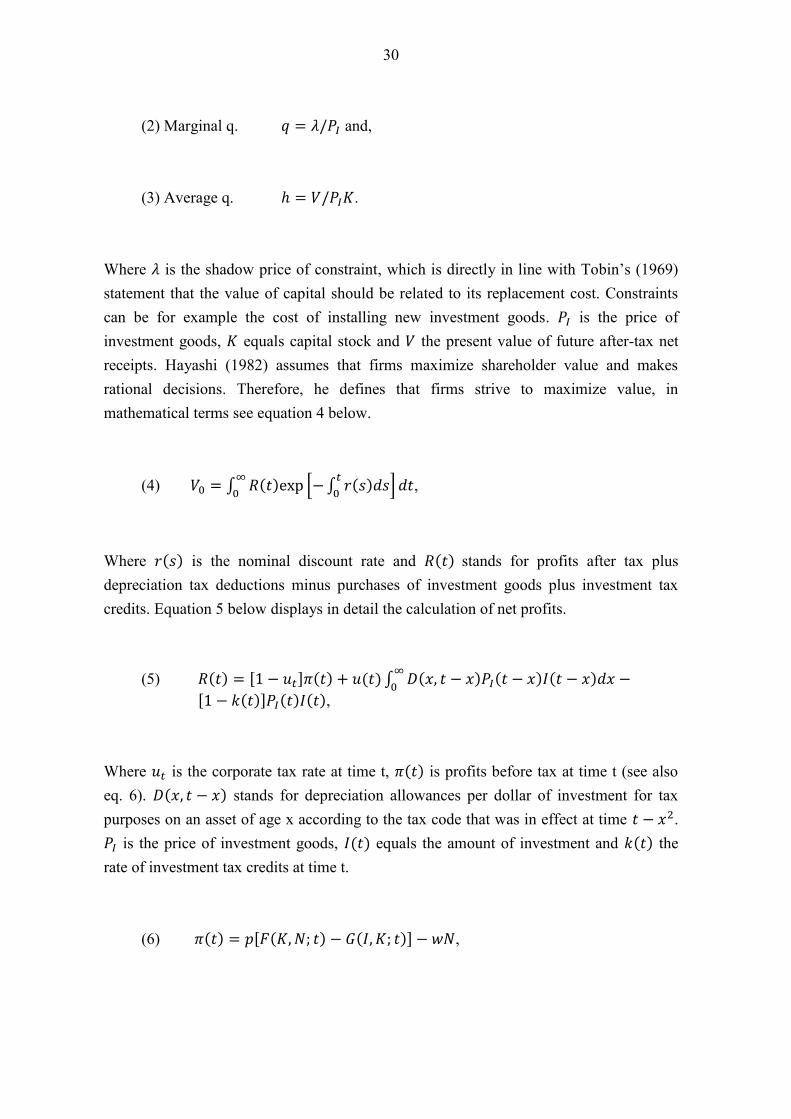
(2) Marginal q. 𝑞 = 𝜆/𝑃𝐼 and,

(3) Average q. ℎ = 𝑉/𝑃𝐼𝐾.

Where 𝜆 is the shadow price of constraint, which is directly in line with Tobin’s (1969) statement that the value of capital should be related to its replacement cost. Constraints can be for example the cost of installing new investment goods. 𝑃𝐼 is the price of investment goods, 𝐾 equals capital stock and 𝑉 the present value of future after-tax net receipts. Hayashi (1982) assumes that firms maximize shareholder value and makes rational decisions. Therefore, he defines that firms strive to maximize value, in mathematical terms see equation 4 below.

(4) 𝑉0 = ∫ 𝑅(𝑡)exp[−∫ 𝑟(𝑠)𝑑𝑠𝑡0 ]∞

0 𝑑𝑡,

Where 𝑟(𝑠) is the nominal discount rate and 𝑅(𝑡)stands for profits after tax plus depreciation tax deductions minus purchases of investment goods plus investment tax credits. Equation 5 below displays in detail the calculation of net profits.

(5) 𝑅(𝑡) = [1 − 𝑢𝑡]𝜋(𝑡) + 𝑢(𝑡) ∫ 𝐷(𝑥, 𝑡 − 𝑥)𝑃𝐼(𝑡 − 𝑥)𝐼(𝑡 − 𝑥)𝑑𝑥 −∞0

[1 − 𝑘(𝑡)]𝑃𝐼(𝑡)𝐼(𝑡), Where 𝑢𝑡 is the corporate tax rate at time t, 𝜋(𝑡) is profits before tax at time t (see also eq. 6). 𝐷(𝑥, 𝑡 − 𝑥) stands for depreciation allowances per dollar of investment for tax purposes on an asset of age x according to the tax code that was in effect at time 𝑡 − 𝑥2. 𝑃𝐼 is the price of investment goods, 𝐼(𝑡) equals the amount of investment and 𝑘(𝑡) the rate of investment tax credits at time t.

(6) 𝜋(𝑡) = 𝑝[𝐹(𝐾,𝑁; 𝑡) − 𝐺(𝐼, 𝐾; 𝑡)] − 𝑤𝑁,

31

Where 𝑝 is the price of the firms output, F is the production function, 𝐾 denotes the capital stock of which a detailed calculation is showed in equation 7. 𝑁 is the vector of input variable factors, e.g. labor and capital. 𝐺 denotes the installation function, which characterizes the cost of installing new investment goods and 𝑤 is the associated vector of input prices.

(7) �̇� = 𝜓(𝐼, 𝐾; 𝑡) − 𝛿𝐾, Where 𝜓 denotes the cost of installing new investment goods and 𝛿 the rate of physical depreciation. In order to simplify the mathematical formulae of value maximization Hayashi (1982) manipulates equation 4 and it reduces to equation 8.

(8) .𝑉(0) = ∫ [(1 − 𝑢)𝜋 − (1 − 𝑘 − 𝑧)𝑝𝐼𝐼]𝑒𝑥𝑝 (−∫ 𝑟𝑑𝑠𝑡0 ) 𝑑𝑡 +∞

0

∫ {𝑢(𝑡)[∫ 𝐷(𝑡 − 𝜐, 𝜐)𝑝𝐼(𝜐)𝐼(𝜐)𝑑𝜐]exp(−∫ 𝑟𝑑𝑠𝑡0 )0

−∞ } 𝑑𝑡∞0 ,

Where, 𝑧(𝑡) = ∫ 𝑢(𝑡 + 𝑥)𝐷(𝑥, 𝑡)exp[−∫ 𝑟(𝑡 + 𝑠)𝑑𝑠]𝑑𝑥𝑥0

∞0 .

After the lengthy derivation of equations 4-6 Hayashi (1982) states that a rational firm strives to maximize 𝑉(0). He takes the first order condition in relation to equation 7 with respect to I and N subject to equation 6. Hence, he concludes with equation 2 and 3, marginal and average q, respectively. Hayashi (1982) combines elegantly the production function and Tobin’s (1969) q-theory into one model, which determines the optimal investment rule, see equation 9. Hayashi (1982) points out that a firms demand curve and production function as well as expectations about future investment tax credits, that affects a firms investment decisions are assimilated into q.

(9) 𝐼 =∝ (𝑞,̃ 𝐾; 𝑡),

Where, 𝑞̃ = 𝑞(1−𝑘−𝑧)

.

32

For the definition of q see equation 2, ‘k’ is defined under equation 5 and the definition of ‘z’ under equation 8. Essentially, the idea is to calculate modified q in order to obtain alfa (∝) by an OLS regression and, therefore, be able to determine the optimal rate of investment defined in equation 9. However, marginal q and modified q are difficult to obtain; thus, Hayashi (1982) proves that marginal q and average q are the same. The equality holds only if four conditions are met: firms operate in perfectly competitive markets, capital is homogenous, investment decisions are made to maximize shareholder value and the production and installation functions are linear and homogenous (Coad 2010).

3.2. Market imperfections and the theory of investment

Hayashi’s (1982) mathematical formulae is flawless, however, the underlying assumptions are strict and rarely, if never holds in the real world. This section will underline how the theoretical framework has been improved in order to better reflect the market conditions faced by firms. Firstly, a discussion on how heterogeneous capital and information asymmetries affect firms and secondly, what kind of agency problems are related to investment.

3.2.1. Heterogeneous capital and information asymmetries

One of the four assumptions in Hayashi’s (1982) theory is that capital is homogeneous both within the firm and among different firms. In other words, if a firm recognizes a profitable investment opportunity and its retained revenues are not sufficient to cover the investment, the firm should be able to raise enough external capital to undertake the investment. Factors, such as, size or age of the firm should not matter. This is not, however, the case, see i.e. Fazzari et al. (1988a), Whited (1992), Galeotti et al. (1994). The ratio between equity and debt has been a subject of research over half a century. The theory of capital homogeneity origins from Modigliani & Miller’s (1958) theorem, according to which a firms capital structure is irrelevant. In perfect market conditions internal and external funds are perfect substitutes of each other. Kraus & Litzenbergerer (1973) introduced the trade-off theory, by which firms balance the ratio between debt and equity. The balancing process is a trade off between increased bankruptcy costs, which rise the more debt a firm bears, and between the larger tax shield increasing debt brings.

33

As in many countries interest rate expenses are tax deductible. Myers & Majluf (1984) introduced the pecking-order-theory according to which firms choose the form of finance based on the most convenient and cost efficient method. Therefore, firms choose to use retained earnings as the first option, after internal funds are exhausted the firm will switch to debt finance. After debt financing becomes costly due to increased bankruptcy costs the firm will choose to raise capital by issuing new shares. Myers (1984: 575) states that there is very little knowledge of corporate funding behavior and how these decisions affect the value of the firm. Leland (1998: 1213) argues that researchers have not been able to explain the behavior of firms on the theoretical foundations of capital structure. Therefore, it would be indecent to advice firms on the optimal capital structure. Furthermore, a large amount of investment literature base their findings on financial constraints on Kraus & Litzenbergs (1973) and Myers & Majluf (1984) theories of capital heterogeneity. Bond & Meghir (1994b) show how capital heterogeneity affects firm investment decisions. To comprehend the investment process under heterogenous capital markets consider a firm with two options: using internal funding or issuing new shares. Figure 1 below illustrates this relationship. (Bond et al. 1994b: 5)

Figure 1. The hierarchy of finance model with no debt finance, (Source: Bond & et al. 1994b: 5).

34

In figure 1 rR denotes the cost of finance from retained earnings and rN the cost of finance from new share issues. 𝐷1𝑎𝑛𝑑𝐷3 describes available investment opportunities to the firm and 𝐼 ̅the maximum level of investment, which can be financed through internal sources. 𝐷1 describes those firms that can fund all of their investment projects by using internal funding. On the other hand 𝐷3 illustrates firms whoms investment projects rate of return is high enough to compensate for the cost of issuing new shares, these firms can also undertake all of their desired projects and are, therefore, not considered to be financially constrained. Furthermore, firms facing investment opportunities described by 𝐷2 consume all their internal funds on accessible investment projects. However, some of the projects are not available as internal funds are insufficient to fund these projects and external funding is too expensive. These firms are considered financially constrained as the rate of return is not high enough to compensate for the cost of issuing new shares. To further elaborate the investment process under different sources of funding, see figure 2 below. (Bond & et al. 1994b: 6–8)

Figure 2. The hierarchy of finance model with debt finance, (Source: Bond & et al. 1994b: 8). As in figure 1 also in figure 2 firms facing investment opportunities 𝐷1 and 𝐷3 are considered unconstrained. Note that these firms do not necessarily spend all available internal funds. They might use debt financing and also pay dividends. For example a firm being in regime 𝐷1 can pay dividends and also issue a corporate bond. The advantage of using debt financing arises from the tax shield the firm will gain, if interest paid on debt

35

is tax deductible. Moreover, firms being in regime 𝐷2 have an additional possibility to firms described in figure 1. Even though these firms have investment opportunities yielding a return somewhere between rR and rN, which is not high enough to cover the costs of issuing new shares, it is possible for these firms to borrow in order to fund investments. However, the disadvantage for firms in regime 𝐷2 is that investors require higher interest rates on additional debt due to increasing probability of default as future profits are expected to be lower for these firms compared to firms in regime 𝐷3. (Bond & et al. 1994b: 4-8) The underlying problem related to financial constraints is considered to be information asymmetries. Whited (1992) describes that firms might be unable or unwilling to disclose important information regarding their investment opportunities. The consequence is that investors overrate the riskiness of investments and require higher premiums. Hence, a wedge between the demand and supply of finance arises. Stiglitz & Weiss (1981) argues that credit does not reach an equilibrium state in the economy due to information asymmetries between lenders and borrowers. The authors present a theoretical framework for their statement. They argue that banks practice adverse selection in order to maximize their profit. Therefore, supply never meets demand. The primary reason for adverse selection is due to the difficulties of properly evaluating lenders. Moreover, the authors stipulate that with perfect and costless information available at all times, no credit rationing would occur. According to Stiglitz et al. (1981) an optimal level of interest exists, where the bank can maximize its profits. Nevertheless, it is only optimal for banks, not for lenders. Figure 3 below demonstrates this.

36

Figure 3. There exists an interest rate which maximizes the expected return to the bank, (Source: Stiglitz et al. 1981: 394). Figure 3 demonstrates that a banks profits decrease in the case of an increasing interest rate. Stiglitz et al (1981) argue that, naturally, different borrowers have different probabilities of default. However, by increasing interest rates only borrowers undertaking riskier projects would apply for a loan, therefore, the increased probability of default in the pool of lenders would decrease the expected return for the bank. Figure 4 illustrates this relationship more closely.

Figure 4. Determination of the market equilibrium, (Source: Stiglitz et al. 1981: 397).

37

In figure 4 𝐿𝑠 denotes loan supply and 𝐿𝐷 loan demand. �̅� stand for the expected return to the bank per dollar loaned and �̂�∗ for the optimal interest rate to maximize the return for the bank. 𝑟𝑚 describes the equilibrium interest rate, �̂� the return on each loan and 𝑍 the excess demand for funds. In figure 4 the upper right quadrant is of special interest. As can be seen a market equilibrium exists at interest rate 𝑟𝑚, where the demand and supply meet. However, banks set the rate at �̂�∗ to maximize their profits. 𝑍 represents the unfortunate lenders who will not be granted a loan even though they would be willing to pay a higher interest rate. Stiglizt & Weiss (1981) argues that a banks competitive equilibrium entails credit rationing, which practically means that even though 𝑟𝑚 would be higher than �̂�∗, not all applicants will be granted a loan. Additionally, the authors argue that collateral does not mitigate credit rationing. They show that by a simple case of two groups of lenders. They assume the wealthy group is willing to take up the most risky projects as they can bear the loss in case of failure, the low wealth group is assumed to be risk averse. Increasing collateral requirements for the low wealth group would increase the banks return. However, a point exists where the higher collateral requirements would drop out individuals from the risk averse low wealth group and switch the weight of the loan portfolio towards riskier individuals. Stiglitz et al. (1891) proves how the positive effects of increasing collateral is offset by the negative effects by a simple two project example, for more details see Stiglitz et al (1981: 402). Financial constraints are harmful for the economy as productive investments, with positive net present value, are forgone due to insufficient finance. This results in lower aggregated production, than could otherwise be produced. Therefore, governments have launched different types of policy interventions to mitigate the issue. For discussion on policy recommendations see i.e. Coad et al. (2010), Fazzari, et al. (1988b), Guariglia (2008) and Hu & Scihiantarelli (1998). 3.2.2. Agency problems in the theory of investment

The principal-agent problem arises when a conflict of interest develops between shareholders (principal) and the chief executive officer (agent). The conflict evolves, mainly due to different desired levels of risk between the two parties. In order to harmonize the desired levels of risk, different types of incentive programs are set in place, such as a stock option plan and alike. (Fama 1980; Pohjola 2009: 67)

38

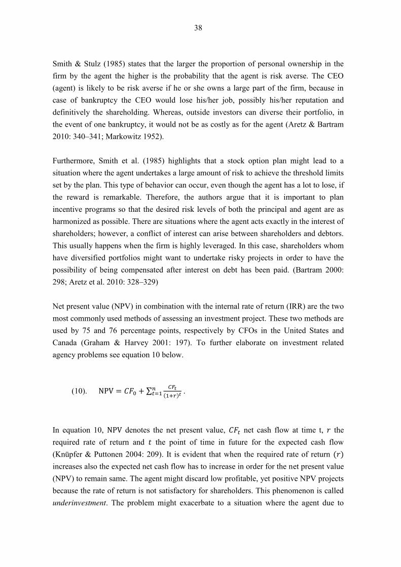
Smith & Stulz (1985) states that the larger the proportion of personal ownership in the firm by the agent the higher is the probability that the agent is risk averse. The CEO (agent) is likely to be risk averse if he or she owns a large part of the firm, because in case of bankruptcy the CEO would lose his/her job, possibly his/her reputation and definitively the shareholding. Whereas, outside investors can diverse their portfolio, in the event of one bankruptcy, it would not be as costly as for the agent (Aretz & Bartram 2010: 340–341; Markowitz 1952). Furthermore, Smith et al. (1985) highlights that a stock option plan might lead to a situation where the agent undertakes a large amount of risk to achieve the threshold limits set by the plan. This type of behavior can occur, even though the agent has a lot to lose, if the reward is remarkable. Therefore, the authors argue that it is important to plan incentive programs so that the desired risk levels of both the principal and agent are as harmonized as possible. There are situations where the agent acts exactly in the interest of shareholders; however, a conflict of interest can arise between shareholders and debtors. This usually happens when the firm is highly leveraged. In this case, shareholders whom have diversified portfolios might want to undertake risky projects in order to have the possibility of being compensated after interest on debt has been paid. (Bartram 2000: 298; Aretz et al. 2010: 328–329) Net present value (NPV) in combination with the internal rate of return (IRR) are the two most commonly used methods of assessing an investment project. These two methods are used by 75 and 76 percentage points, respectively by CFOs in the United States and Canada (Graham & Harvey 2001: 197). To further elaborate on investment related agency problems see equation 10 below.

(10). NPV = 𝐶𝐹0 + ∑ 𝐶𝐹𝑡(1+𝑟)𝑡

𝑛𝑡=1 .

In equation 10, NPV denotes the net present value, 𝐶𝐹𝑡 net cash flow at time t, 𝑟 the required rate of return and 𝑡 the point of time in future for the expected cash flow (Knüpfer & Puttonen 2004: 209). It is evident that when the required rate of return (𝑟) increases also the expected net cash flow has to increase in order for the net present value (NPV) to remain same. The agent might discard low profitable, yet positive NPV projects because the rate of return is not satisfactory for shareholders. This phenomenon is called underinvestment. The problem might exacerbate to a situation where the agent due to

39

self-interest or on behalf of the interest of shareholders discard positive NPV projects and accept negative NPV projects. This is called asset substitution or for a risk shifting problem. Debtors usually recognize the opportunistic behavior and require a higher interest rate on corporate bonds and/or covenants. A typical covenant can be for example that a firm is not allowed to exceed a certain debt to equity ratio. (MacMinn 1987: 672; Aretz et al. 2010: 328–329) Smithson, Smith & Wilford (1995) conclude that by hedging it is possible to reduce or eliminate underinvestment and the risk shifting problem. By a practical example they demonstrate that if a firm wants to increase the amount of debt and still maintain their credibility among debtors the firm should commit to hedge against interest rate risk. This allows the firm to take full advantage of additional debt in form of an increased tax shield and at the same time avoid increased bankruptcy costs and underinvestment.

3.3 The Evolutionary theory

The theoretical framework for the evolutionary theory of investment is built upon Ronald Fisher’s (1930) conclusions of population genetics. An implementation of a biological theory into economic literature has its roots in the idea of the survival of the ‘fittest’. Also, criticism towards the fundamental principle of rationality of individuals and firms is an essential part of the evolutionary theory. One to point out the irrationality to expect rationality among firms was Alchian (1950). He argued that in the state of uncertainty of the future, firms are unable to act in accordance with the prevailing assumptions that firms always seek to maximize profit under perfect information and well established expectations of future profits. Therefore, a natural selection of firms exists, where random chance plays a crucial role. Alchian (1950) argues that in a certain economic environment some firms have relative advantage compared to others; however, the environment can change and shift the advantageous position to another group of firms. He underlines that adaptability to changes is important as well as being able to imitate best practices of successful firms in order make positive profits and to survive. Moreover, the importance of Alchian’s (1950) study is considered to be the alternative interpretation of firm behavior compared to the mainstream literature, where rationality and perfect information are assumed.

40

The evolutionary theory has been conceptualized among others by Coad (2010). He shows how Fishers (1930) theory works in the economic context. He argues that firms choose their level of investment based on current financial performance, because of the inability to forecast accurately future profits. Equation 11 below clarifies the evolutionary approach to investment. (11) 𝛿𝑥𝑖 = 𝛼𝑥𝑖(𝐹𝑖 − �̅�), Where 𝛿 denotes the variation in the infinitesimal interval 𝑡, 𝑡 + 𝛿𝑡 and 𝑥𝑖 is a measure of fixed assets, firm size, or market share of firm 𝑖 in a population of competing firms. 𝐹𝑖 is the level of fitness of firm 𝑖, measured as relative performance or relative productivity and �̅� is the average fitness in the population. (Coad 2010: 210) Some evident conclusions can be drawn from equation 11. If a firm is able to maintain a level of fitness (𝐹𝑖) above the average firm (�̅�) in the population, then the firm will grow and increase its market share (Coad 2010: 210). Fitness can be proxied by for example profits or relative productivity. If a firm is operating in a competitive market and does not have a unique product or service, however it has more efficient production processes, obviously it will have a relative advantage over the average firm in the population. Jovanovic (1982) argues that firms are not necessarily efficient from the beginning; instead they learn to improve their efficiency overtime. Some firms survive the learning path and some do not and are, therefore, forced to exit. However, it does not mean that a firm can reach a mature face where the improving has come to its end. Actually, it is the opposite, if one considers Alcihan’s (1950) theory of a constantly changing environment where firms are forced to adapt to changing conditions, a firm can never reach a mature state. It is an infinite ongoing process. Metcalfe (1994) develops a detailed and comprehensive framework for the evolutionary concept. He states that the dynamic selection process in terms of increasing returns is a co-dynamic system with the aggregated increase in the growth of the economy. Metcalfe (1994) argues that the properties of a stationary equilibrium economy are irrelevant. Of actual importance is the process of a dynamic change and the understanding of the underlying factors contributing to change. Metcalfe (1994) shows how the selective process under competition yields increasing returns overtime for firms with superior

41

behavior. He demonstrates by a simple example of two competing firms, under various conditions, how the Fisher’s principle drives the dynamic process to improving the economy overtime, see figure 5. However, he adds, that the selection process is not under all circumstances improving the economy, see figure 6.

Figure 5. Relative competitive advantage. (Source: Metcalfe 1994:340).

Figure 6. Different circumstances in the economy. (Source: Metcalfe 1994:341).

42

In figure 5 and 6 ℎ𝑖 denotes unit cost and 𝑠𝐼 market share. In figure 5 two competing firms operate on the same market with fixed industry level output. Firm ones improving production process is illustrated by the dashed line. What can be seen from figure 5 is that firm one will increase its market share on the expense of firm two. The only way firm two can stay in the market is if the product price is higher than ℎ2. This is of course, unlikely unless the demand is higher than what can be supplied. In the long run firm one is able to invest with an increasing speed in new machinery and overtake a larger market share from firm two. In a more realistic economy with several participants, the price should converge to ℎ1, unless market circumstances create a lock, where superior technology is unable to transcend inferior technology. Metcalfe (1994) Figure 6 describes a situation where the selection process can lead to use of inferior technology. If firm one is not able to capture the critical market share of 𝑠1∗ the selection process will lead to competitive advantage of firm two, which use low-grade technology. This type of economy is reflected by exceptionally strong economies of scale. The selection effect is outweighed by the scale effects on unit cost levels. If firm one is entering the market, and it requires extensive investments to reach the critical market share of 𝑠1∗ Metcalfe (1994) argues that public subsidies may be the only way of establishing the superior technology. To summarize the evolutionary theory; some contradictory points have been made by Metcalfe (1994) and Coad (2010) regarding financial constraints. Coad (2010) argues that firms incorporating vital skills to survive in a competitive market are better in recognizing profitable investment opportunities and are also better coped in obtaining finance for their projects than less skilled firms. However, in the light of Metcalfe (1994) description of exceptionally strong economies of scale, it could be argued that firms do face financial constraints, and government subsidies would be justified. Nevertheless, a common understanding among Alchian (1950), Coad (2010), Hopenhayn (1992), Jovanovic (1982) and Metcalfe (1994) is that firm behavior is not driven by an optimization of maximizing profits in an economy of equilibrium. Rather, the economy is a dynamic environment, where firms strive to survive and grow.

43

4. DATA AND METHODOLOGY

A vast amount of research has been conducted both using Tobin’s q and cash flow explaining investment. Additionally, previous literature has focused on finding the correct measure of q and in recognizing financial constraints. Over decades of investment research three paradigms have evolved, the q-theory, the imperfect markets approach and the evolutionary theory. The imperfect markets approach has recognized cash flow as a meaningful explanatory variable. However, contradictory empirical evidence in q and cash flow as explanatory variables has been reported. More recent work such as Botazzi et al. (2008) and Coad (2007; 2010) have questioned the underlying assumptions of the q-theory and examined investment from a different perspective. This chapter outlines the data and methodology which are used in the empirical part. The source of the data and the selection process are thoroughly revised. Furthermore, a discussion on the quality and suitability of the data for the empirical part is presented. Numerous investment studies have been conducted on U.S. data. Therefore, an emphasis on European data, focusing on the German economy is considered to be of importance.

4.1. Data

The data is obtained from Thomson Reuters Worldscope database. The initial sample contains 2 317 listed German firms. The data includes eleven years of observations from 2004 to 2014. Twelve different variables are extracted for all firms; the variables are presented in table 1. Firms with SIC codes between 60 and 67 are excluded. These firms are finance, insurance and real-estate firms. After controlling for SIC codes (60–67) and for sufficient observations on all the variables the remaining sample consists of an unbalanced panel of 779 firms.

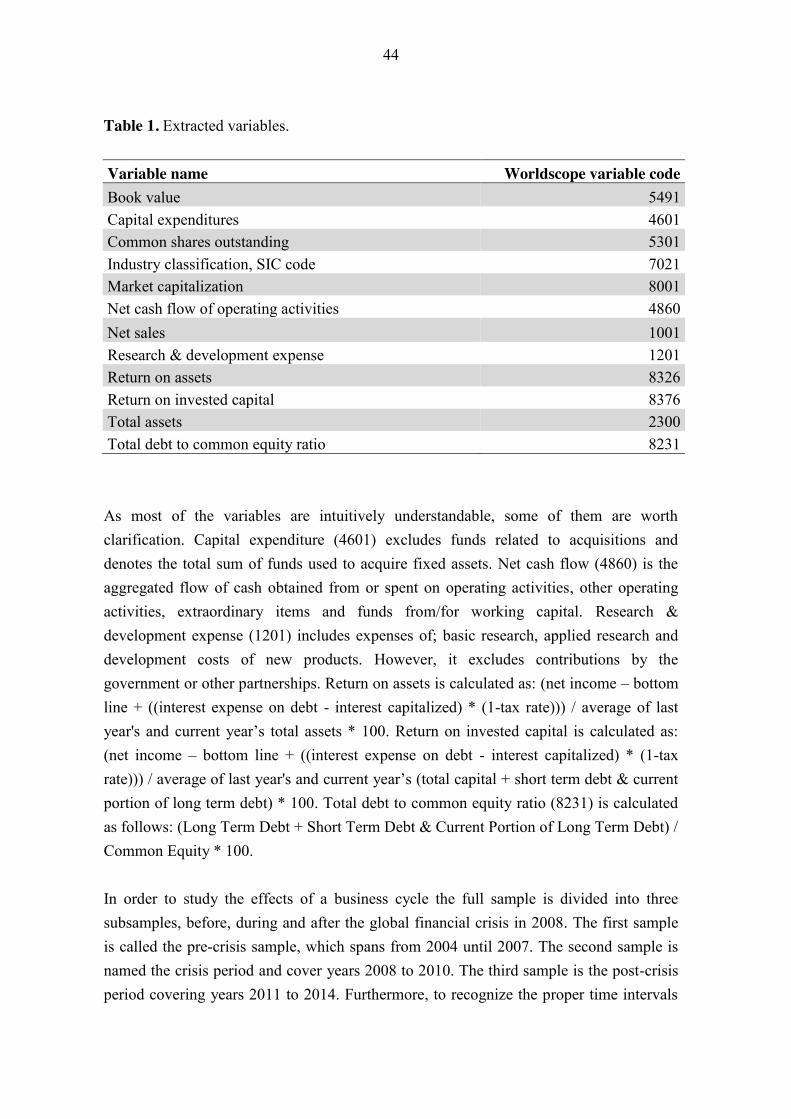
44

Table 1. Extracted variables. Variable name Worldscope variable code Book value 5491 Capital expenditures 4601 Common shares outstanding 5301 Industry classification, SIC code 7021 Market capitalization 8001 Net cash flow of operating activities 4860 Net sales 1001 Research & development expense 1201 Return on assets 8326 Return on invested capital 8376 Total assets 2300 Total debt to common equity ratio 8231 As most of the variables are intuitively understandable, some of them are worth clarification. Capital expenditure (4601) excludes funds related to acquisitions and denotes the total sum of funds used to acquire fixed assets. Net cash flow (4860) is the aggregated flow of cash obtained from or spent on operating activities, other operating activities, extraordinary items and funds from/for working capital. Research & development expense (1201) includes expenses of; basic research, applied research and development costs of new products. However, it excludes contributions by the government or other partnerships. Return on assets is calculated as: (net income – bottom line + ((interest expense on debt - interest capitalized) * (1-tax rate))) / average of last year's and current year’s total assets * 100. Return on invested capital is calculated as: (net income – bottom line + ((interest expense on debt - interest capitalized) * (1-tax rate))) / average of last year's and current year’s (total capital + short term debt & current portion of long term debt) * 100. Total debt to common equity ratio (8231) is calculated as follows: (Long Term Debt + Short Term Debt & Current Portion of Long Term Debt) / Common Equity * 100. In order to study the effects of a business cycle the full sample is divided into three subsamples, before, during and after the global financial crisis in 2008. The first sample is called the pre-crisis sample, which spans from 2004 until 2007. The second sample is named the crisis period and cover years 2008 to 2010. The third sample is the post-crisis period covering years 2011 to 2014. Furthermore, to recognize the proper time intervals

45

the implied volatility VDAX risk measure is used. The underlying stock index for VDAX is DAX30 and is, therefore, well suited to measure investor sentiment regarding German firms.

For a non-professional implied volatility can be difficult to understand only by interpreting the definition. In finance volatility describes the standard deviation around an instrument’s price changes in a given time period, for instance one year. Implied refers in this context to an obtained volatility value derived from an option-pricing model, such as the Black-Scholes (1973) and Merton (1973) model, where instead of price, volatility is the unknown factor. By inputting the current market price into the model it yields the implied volatility. Hence, it describes the expected volatility of market participants and is also defined as the ’market fear gauge’ (Whaley 2000).

Because the sample firms are listed, VDAX should be a good indicator of current uncertainty faced by the firms. Therefore, it can be considered to be a valid indicator of determining different phases of the business cycle. In addition to VDAX, support for the time interval selection process is drawn from the CDAX index, which represents all the listed firms on the Frankfurt stock exchange. Figure 7 presents VDAX values from 2005 until 2014 and the corresponding subsample selection criteria. The pre- and post-crisis samples are both four years long, and the crisis period covers three years. It is not, however, clear when the crisis period can be considered to be over. As can be seen from figure 7, in 2011 a fairly high peak of VDAX has been recorded. Though, the peak is significantly lower than the one recorded in 2008. Therefore, year 2011 is included in the post-crisis period.

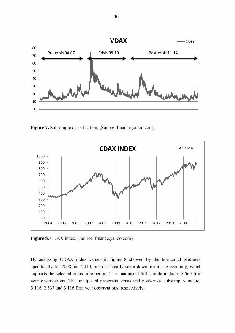
46

Figure 7. Subsample classification, (Source: finance.yahoo.com).

Figure 8. CDAX index, (Source: finance.yahoo.com). By analyzing CDAX index values in figure 8 showed by the horizontal gridlines, specifically for 2008 and 2010, one can clearly see a downturn in the economy, which supports the selected crisis time period. The unadjusted full sample includes 8 569 firm year observations. The unadjusted pre-crisis, crisis and post-crisis subsamples include 3 116, 2 337 and 3 116 firm year observations, respectively.

0

10

20

30

40

50

60

70

80

VDAX Close

Pre-crisis 04-07 Crisis 08-10 Post-crisis 11-14

0

100

200

300

400

500

600

700

800

900

1000

2004 2005 2006 2007 2008 2009 2010 2011 2012 2013 2014

CDAX INDEX Adj Close

47

Table 2. Descriptive statistics of key variables. No industry adjusting CF ROA ROI Q Panel A: full sample 04-14 Mean 0.04 2.47 4.10 2.39 Median 0.06 4.11 6.28 1.68 Maximum 0.38 20.59 33.23 20.74 Minimum -0.75 -35.06 -56.16 0.30 Std. Dev. 0.16 9.43 14.53 2.35 Observations 6112 5986 5912 5866

Panel B: pre-crisis 04-07 Mean 0.03 3.11 5.49 2.67

Median 0.06 4.48 7.20 1.92 Maximum 0.42 21.48 43.18 19.52 Minimum -0.65 -33.15 -50.28 0.38 Std. Dev. 0.16 9.28 14.72 2.44 Observations 2345 2355 2330 2259

Panel C: crisis 08-10 Mean 0.03 1.62 2.92 2.17

Median 0.06 3.78 5.65 1.44 Maximum 0.60 19.85 30.54 27.57 Minimum -5.32 -39.64 -58.74 0.26 Std. Dev. 0.29 10.36 15.17 2.65 Observations 1804 1719 1693 1727

Panel D: post-crisis 11-14 Mean 0.04 2.40 3.53 2.29

Median 0.06 4.08 6.12 1.63 Maximum 0.36 19.26 29.30 16.83 Minimum -0.81 -33.74 -61.34 0.29 Std. Dev. 0.16 8.85 14.16 2.10 Observations 1963 1914 1891 1880 Notes: Cash flow (CF) is scaled by each firms total assets. Table 2 shows descriptive statistics on industry adjusted cash flow, return on assets, return on investment and the debt to equity ratios for the full and subsamples. All the key variables include outliers. Furthermore, some extreme values are identified in the cash flow variable. However, it is not obvious whether these extreme values are due to calculation errors in the database or because of some abnormal events in the firms.

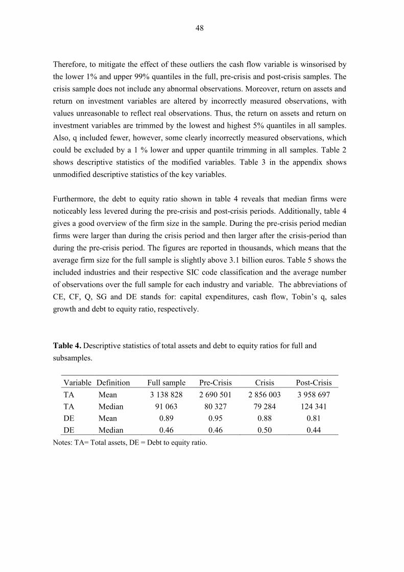
48

Therefore, to mitigate the effect of these outliers the cash flow variable is winsorised by the lower 1% and upper 99% quantiles in the full, pre-crisis and post-crisis samples. The crisis sample does not include any abnormal observations. Moreover, return on assets and return on investment variables are altered by incorrectly measured observations, with values unreasonable to reflect real observations. Thus, the return on assets and return on investment variables are trimmed by the lowest and highest 5% quantiles in all samples. Also, q included fewer, however, some clearly incorrectly measured observations, which could be excluded by a 1 % lower and upper quantile trimming in all samples. Table 2 shows descriptive statistics of the modified variables. Table 3 in the appendix shows unmodified descriptive statistics of the key variables. Furthermore, the debt to equity ratio shown in table 4 reveals that median firms were noticeably less levered during the pre-crisis and post-crisis periods. Additionally, table 4 gives a good overview of the firm size in the sample. During the pre-crisis period median firms were larger than during the crisis period and then larger after the crisis-period than during the pre-crisis period. The figures are reported in thousands, which means that the average firm size for the full sample is slightly above 3.1 billion euros. Table 5 shows the included industries and their respective SIC code classification and the average number of observations over the full sample for each industry and variable. The abbreviations of CE, CF, Q, SG and DE stands for: capital expenditures, cash flow, Tobin’s q, sales growth and debt to equity ratio, respectively. Table 4. Descriptive statistics of total assets and debt to equity ratios for full and subsamples.

Variable Definition Full sample Pre-Crisis Crisis Post-Crisis TA Mean 3 138 828 2 690 501 2 856 003 3 958 697 TA Median 91 063 80 327 79 284 124 341 DE Mean 0.89 0.95 0.88 0.81 DE Median 0.46 0.46 0.50 0.44

Notes: TA= Total assets, DE = Debt to equity ratio.

49

Table 5. Industry classification and average number of observations in each industry and variable.

SIC Description CE R&D CF ROI ROA Q SG DE 10-14 Mining 10 5 11 12 12 10 10 12 15-17 Construction 14 5 13 15 16 14 15 16 20-39 Manufacturing 285 171 284 305 308 276 299 298 40-49 Trans. & Pub. utilities 47 12 48 51 51 47 51 50 50-51 Wholesale Trade 16 4 17 18 19 17 18 18 52-59 Retail Trade 19 2 19 19 20 18 20 20 70-89 Services 157 65 162 177 179 162 173 169

Total 549 265 555 597 605 544 587 582

Notes: Trans. & Pub. utilities = Transportation & public utilities. The sample contains a fair amount of German firms from a wide variety of industries, gathered from a trustworthy database. Finance, insurance and real-estate firms are excluded from the sample due to the peculiar nature of these business areas. The sample period covers an economic decline, which gives a good opportunity to study the effects of a business cycle. Although, the change from a downward trend to an upward trend is a transitionary phase without a distinct date, the subsamples should capture the variations adequately. The variation in leverage ratios and total assets supports the selected time periods for the subsamples. The sample does not account for mergers and acquisitions (M&A), and neither for entries or exits. However, considering the amount of firms and observations M&A’s should not affect the outcome of the results. Additionally, exits and entries are considered a natural part of the evolutionary theory and, therefore, excluding them would impair the sample rather than improve it. Overall the diverse sample, covering eleven years is well suited to examine the evolutionary theory of investment. However, taking into account the large size of the sample firms, no conclusions of small firm behavior can be made based on this data. Additionally, the manufacturing and services sectors accounts for the majority of the total number of observations.

50

4.2. Methodology

The methodology in this thesis is based on theoretical work conducted among others by Alchian (1950), Jovanovic (1982), Metcalfe (1994) and Coad (2010). The basic principle lays in Fishers (1930) evolutionary approach, which has been formalized into an investment framework (see equation 11). The core idea is to test the theory of the selection process in the German economy. Furthermore, if weaker firms invest less compared to fitter firms? Three different proxies of firm fitness are constructed by industry adjusting each firms yearly cash flow, return on assets and return on investment to the industry median. This captures the competitive angle in an economy and takes also into account the diversity of different industries. By deducting the median value based on the two digit SIC codes, describes how high or low the three variables are compared to industry peers. Furthermore, two types of dependent variables for investment are used: Capital expenditures and research & development expenses. Additionally, three control variables are used in all regressions: Tobin’s q, sales growth and the debt to equity ratio. The purpose of the two latter variables is to capture the impact of growth and leverage. Tobin’s q is included to estimate whether the traditional q-theory has any explanatory power. In order to examine whether fitter firms invest more compared to weaker firms, three groups are constructed by dividing the three proxies of fitness into separate quantiles: low, medium and high. Observations in the lowest group include industry adjusted values < 25th quantile, the medium group include observations > 25th and < 75th quantile, and the highest group include observations > 75th quantile. Equations 12 to 17 describe different binary panel least square regressions measuring the impact of industry adjusted cash flow, industry adjusted return on assets and industry adjusted return on investment on capital expenditures and research & development expenses.

(12). 𝐶𝐸 = α + 𝛽1𝐷𝐿𝑂𝑊 + 𝛽2𝐷𝐻𝐼𝐺𝐻 + 𝛽3𝑄 + 𝛽4𝑆𝐺 + 𝛽5𝐷𝐸 + 𝜀𝑖𝑡.

(13). 𝐶𝐸 = α + 𝛽1𝐷𝐿𝑂𝑊 + 𝛽2𝐷𝑀𝐸𝐷 + 𝛽3𝑄 + 𝛽4𝑆𝐺 + 𝛽5𝐷𝐸 + 𝜀𝑖𝑡.

(14). 𝐶𝐸 = α + 𝛽1𝐷𝑀𝐸𝐷 + 𝛽2𝐷𝐻𝐼𝐺𝐻 + 𝛽3𝑄 + 𝛽4𝑆𝐺 + 𝛽5𝐷𝐸 + 𝜀𝑖𝑡.

51

(15). 𝑅&𝐷 = α + 𝛽1𝐷𝐿𝑂𝑊 + 𝛽2𝐷𝐻𝐼𝐺𝐻 + 𝛽3𝑄 + 𝛽4𝑆𝐺 + 𝛽5𝐷𝐸 + 𝜀𝑖𝑡.

(16). 𝑅&𝐷 = α + 𝛽1𝐷𝐿𝑂𝑊 + 𝛽2𝐷𝑀𝐸𝐷 + 𝛽3𝑄 + 𝛽4𝑆𝐺 + 𝛽5𝐷𝐸 + 𝜀𝑖𝑡.

(17). 𝑅&𝐷 = α + 𝛽1𝐷𝑀𝐸𝐷 + 𝛽2𝐷𝐻𝐼𝐺𝐻 + 𝛽3𝑄 + 𝛽4𝑆𝐺 + 𝛽5𝐷𝐸 + 𝜀𝑖𝑡. In equations 12 to 17 𝐶𝐸 and 𝑅&𝐷 denotes capital expenditures and research & development expenses, respectively, which are scaled by the firms total assets in order to eliminate the highly different levels of observations caused by the size of the firms. 𝐷𝐿𝑂𝑊, 𝐷𝑀𝐸𝐷, and 𝐷𝐻𝐼𝐺𝐻 represents dummy groups, which are referred to as group 1 to 3, respectively, describing industry adjusted cash flow, ROA or ROI at time 𝑡0 or 𝑡−1. Equations 12 to 17 include three control variables. The 𝑄 value controls for the traditional investment theory, according to which investment is related to the replacement cost of capital. Q is calculated by dividing the market value per share with the book value per share. 𝑆𝐺 denotes sales growth is calculated by subtracting the current year sales from the previous year sales and by dividing it by the previous year sales. Total annual sales figures are obtained for 2003 in order to calculate the sales growth for year 2004. Moreover, sales growth affects the level of cash flow and could, therefore, have an impact on investment. For example, Fazzari et al. (1988a), finds sales growth as a significant factor in their study. Contrary to the Modigliani & Miller (1958) theorem, the capital structure of firms is not irrelevant. Highly leveraged firms suffer from bankruptcy costs and agency problems (see Aretz et al. 2010 and MacMinn 1987). To control for leverage the debt to equity ratio, denoted as 𝐷𝐸, is included in the model. This study strives to test whether fitter firms, which encompass unique skills, are able to invest more compare to weaker firms. Three proxies of fitness are used and two dependent variables measuring investment. The following hypothesis is formulated to test the relationship between fitter and weaker firms.

𝐻1:𝛽1 = 𝛽2.

52

Hypothesis 1 is tested by running models 12 to 17, and if the variables are significant they will additionally be tested by the wald-test. Furthermore, if only one of the variables is significant and of correct sign hypothesis 2 will be tested.

𝐻2:𝛽j = 0. It can be argued that it is reasonable to admit that the strict assumptions regarding the q-theory of investment cannot be fulfilled. Furthermore, to assume that firms are able to accurately forecast future profits with an infinite time horizon is not realistic. Thus, the evolutionary approach does not assume firms to be fully aware of all possible investment opportunities and to be able to evaluate precisely the net present value of these opportunities. Moreover, firms enhance over time their internal evaluation processes and become better in recognizing profitable investment opportunities. Consequently, fitter firms should have higher cash flow and higher profitability ratios compared to their industry peers. Thus, these firms are expected to be able to invest more compared to weaker firms.

53

5. EMPIRICAL RESULTS

The empirical results in this thesis were obtained by applying the methodologies covered in the previous chapter. Firstly, results of the full sample are presented and secondly, of the subsamples. Lastly, a discussion on the robustness of the results is included.

5.1. Empirical results of the full and subsamples

Table 6 describes the empirical results of the full sample. Both independent variables, capital and R&D -expenditures are presented along with the key explanatory variables. Interestingly, the findings are contradictory, although, the independent variables are expected to respond similarly to the predicted variables. In panel 1 Industry adjusted cash flow is of correct sign in all models when it is regressed on capital expenditures. Models 1 to 3 all confirm that firms with higher cash flow compared to their industry peers have a positive impact on capital expenditures. Model 2 displays strongest evidence for this relationship. Firms being in low and medium groups invest less compared to firms with excessive cash flow compared to their industry peers. The same relationship is also confirmed when industry adjusted cash flow is lagged by one year. However, the coefficients are smaller and less significant compared to current industry adjusted cash flow. Hypothesis 2 can be rejected in all models with industry adjusted cash flow as the explanatory variable with a 5% significance level. Low and medium groups in model 2 are not statistically different from each other, meaning that these two groups are both investing less than group 3. However, the lowest group is not investing less than the medium group, even though the coefficients show slightly different values. In panel 1 Industry adjusted return on assets and return on investment show similar behavior as industry adjusted cash flow. However, these two variables are only significant when regressed with a one year lag. This is expected, as cash flow has primarily been recorded, in previous studies, to be significant in measuring current financial performance on investment.

54

Table 6. Empirical results of the full sample. Full sample 2004-2014 Lag t-1 Model 1 Model 2 Model 3 Model 4 Model 5 Model 6

Dependent variable: Capital expenditures/total assets.

Panel 1: Independent variables.

Low CF -0.002 -0.006***

-0.001 -0.004 Medium CF

-0.004*** 0.001

-0.002* 0.003

High CF 0.005***

0.006*** 0.005**

0.007***

Low ROA -0.000 -0.002

-0.002 -0.007*** Medium ROA

-0.001 0.000

-0.005*** 0.001

High ROA 0.002

0.003 0.005***

0.007***

Low ROI 0.000 -0.000

-0.002* -0.009*** Medium ROI

-0.002 -0.001

-0.006** 0.003*

High ROI 0.001

0.001 0.007***

0.009***

Dependent variable: R&D expenditures/total assets. Panel 2: Independent variables.

Low CF 0.008*** 0.009***

0.006** 0.008*** Medium CF

0.001 -0.008***

0.002 -0.006**

High CF -0.001

-0.009*** -0.002

-0.008***

Low ROA 0.011*** 0.010***

0.006*** 0.010*** Medium ROA

0.003*** -0.005***

0.004*** -0.004***

High ROA -0.003***

-0.008*** -0.003***

-0.006***

Low ROI 0.010*** 0.010***

0.009*** 0.012*** Medium ROI

0.002 -0.08***

0.003 -0.009***

High ROI -0.002**

-0.010*** -0.003

-0.011***

Notes: *, **, *** = 10, 5 and 1% significance levels, respectively. Fixed cross-section and period effects and coef. covariance method = White cross-section. The independent variables are industry adjusted by deducting the industry median value by the 2 digit SIC codes. Regressions in panel 2 are of reduced rank.

55

In panel 1 and model 5 for industry adjusted return on assets, hypothesis one cannot be rejected, however, hypothesis two can be rejected for both low and medium groups with a 1 % significance level. Very similar results are obtained in panel 1 for industry adjusted return on investment; the significant variables are in the lagged models 4 to 6. Again, firms having lower industry adjusted return on investment compared to their industry peers are able to invest less compared to firms belonging to group three. Hypothesis one is not supported by model 4, implying that firms belonging to group 1 invest less compared to the medium group and firms in group 3 invest more compared to the medium group. Additionally, hypothesis one is rejected in models 5 and 6 with 10 % and 1 % significance levels, respectively. Furthermore, the control variables remain mainly insignificant or of very small magnitude, when being statistically significant. Furthermore, the results in panel 1 show strong evidence that firms being fitter in form of having higher cash flow, return on assets and return on investment compared to their industry peers are able to invest more compared to weaker firms. Not only do these firms invest more, it seems that firms being in group one has a negative impact on capital expenditures. These findings support strongly the evolutionary theory, where fitter firms are able to grow and invest more, whereas, weaker firms are deteriorating. Results in panel 2 measuring the three proxies of fitness on R&D expenditures contradict the findings in panel 1. The high and medium groups are statistically significant and of negative sign. Implying that firms, which have an excessive cash flow position compared to their industry peers or higher return on assets and return on investment seem to have a negative impact on R&D expenditures. These findings are aberrant, as previous research conducted e.g. by Himmelberg & Petersen (1994), finds that R&D is related to internal funding, therefore, one could expect excessive cash flow to be positively correlated with R&D expenditures. It is, however, possible that the sample period in this study might have a peculiar effect on the results. Brown, Fazzari & Petersen (2009) studied the 1990s R&D boom in U.S. Their results reveal that a significant portion of the aggregated R&D expenditures are contributed by young high-tech firms. The authors conclude that financial systems play an important role in the growth of an economy. Market-driven economies such as the U.S. were able to provide a substantial amount of funding for young high-tech firms through stock exchanges, whereas bank-driven economies such as Germany and France, failed to do so. At least in the same extent as in the U.S. (Brown et al. 2009)

56

High-tech firms in this thesis does account only for a small portion compared to the total number of firms. Brown et al. (2009) findings show that financial variables such as cash flow did not show statistically or economically significant coefficients for mature firms outside the high-tech industry. Considering Brown et al. (2009) findings, the sample period under investigation and the character of the firms in this thesis, it could provide an explanation for the negative effect of the financial variables regressed on R&D. It is possible, that Germany has faced a similar, however, smaller trend in R&D as the one recorded in U.S. The sample period in this thesis begins, when Brown et al. (2009) considers the R&D boom to have plummeted. One explanation could be that firms have reduced their R&D expenditures compared to pre-2004 levels during the time period used in this study and, therefore, the results provided in table 6 show a negative effect on the proxies for firm fitness. These interpretations are, however, vague and cannot be confirmed. Additionally, it does not explain why fitter firms seem to have a negative impact on R&D expenditures.

57

Table 7. Empirical results of subsamples with capital expenditures as the dependent variable.

Panel Independent variables Model 1 Model 2 Model 3 3 Pre-crisis

Low CF 0.003 0.002

Medium CF

-0.002 -0.003

High CF 0.002

-0.002

Low ROA 0.002 0.001

Medium ROA

-0.001 -0.002

High ROA 0.001

-0.001

Low ROI -0.000 0.001

Medium ROI

-0.002 -0.002**

High ROI -0.002*

-0.001

4 Crisis

Low CF -0.004** -0.006

Medium CF

-0.002 0.004**

High CF 0.002

0.006

Low ROA 0.007** 0.006***

Medium ROA

-0.001 -0.007**

High ROA 0.001

-0.006***

Low ROI 0.005 0.009***

Medium ROI

0.004 -0.005

High ROI -0.004

-0.009***

5 Post-crisis

Low CF -0.003*** -0.010*** Medium CF

-0.007** 0.003***

High CF 0.007**

0.010***

Low ROA -0.002 -0.003*

Medium ROA

0.001 0.002

High ROA 0.001

0.003*

Low ROI -0.002 -0.003**

Medium ROI

-0.001* 0.002***

High ROI 0.001

0.003**

58

Table 8. Empirical results of subsamples with R&D as the dependent variable.

Panel Independent variables Model 1 Model 2 Model 3 6 Pre-crisis

Low CF 0.002 0.001

Medium CF

-0.001 -0.002

High CF 0.001

-0.001

Low ROA 0.009*** 0.008***

Medium ROA

0.000 -0.008***

High ROA -0.000

-0.008***

Low ROI 0.008*** 0.01***

Medium ROI

0.002 -0.008***

High ROI -0.002

-0.01***

7 Crisis

Low CF 0.002 0.011***

Medium CF

0.008*** -0.002

High CF -0.008***

-0.010***

Low ROA 0.011*** 0.013***

Medium ROA

0.002*** -0.011***

High ROA -0.002***

-0.013***

Low ROI 0.011*** 0.014***

Medium ROI

0.003*** -0.011***

High ROI -0.003***

-0.014***

8 Post-crisis

Low CF 0.000 -0.002

Medium CF

-0.002 -0.000

High CF 0.002

0.002

Low ROA 0.002 0.005**

Medium ROA

0.005* -0.000

High ROA -0.005**

-0.005**

Low ROI 0.002 0.005**

Medium ROI

0.003 -0.002**

High ROI -0.001

-0.005**

59

Notes for table 7 and 8: *, **, *** = 10, 5 and 1% significance levels, respectively. Fixed cross-section and period effects and coef. covariance method = White cross-section. The independent variables are industry adjusted by deducting the industry median value by the 2 digit SIC codes. All regressions in panel 3 to 8 are of reduced rank.

Based on table 7 and panel 3 it can be observed that the pre-crisis period has almost no significant coefficients. Only models 1 and 3 with industry adjusted return on investment as the explanatory variable shows statistically significant coefficients, however, with incorrect signs. Panel 4 and 5 regarding industry adjusted cash flow, confirms the same pattern as in the full sample. Firms with higher cash flow compared to their industry peers have a positive impact on capital expenditures. Hypothesis one can be rejected with a 5% significance level in models 1 and 3 in panel 4. The post-crisis period shows the strongest evidence for the argument that fitter firms invest more compared to weaker firms. In panel 5 hypothesis one can be rejected for all models with industry adjusted cash flow as the explanatory variable. Model 1 and 2 can be rejected with a 1% significance level and model 3 with a 5% significance level. In table 7 industry adjusted return on assets and return on investment are generally confirming the same findings as with industry adjusted cash flow, except during the crisis period, when the signs are reversed. Table 8 displays the results for the subsamples using R&D expenditures as the dependent variable. Industry adjusted cash flow is insignificant in both the pre-crisis period and post-crisis period. During the crisis period the coefficients are significant, however, of incorrect sign. Industry adjusted return on assets and return on investment show stronger significance in panels 6 to 8; these variables are also negative for firms belonging to group 3.

5.2 Robustness of the results

The results in panel one can be considered robust, as enough observations for reliable results are obtained also for the lagged models. However, it should be reminded that the majority of the observations are from two sectors, manufacturing and services. Therefore, the results should mainly be interpreted as findings within these two sectors.

60

The most plausible explanation for the three proxies of firm fitness responding negatively to R&D expenditures is the lack of sufficient observations. The regressions including R&D expenditures as the dependent variable in the full sample include observations between 435 and 440 for the unlagged models; all of these regressions are of reduced rank. Practically, it means that the results are unreliable. In comparison, when regressing capital expenditures on the three different proxies of fitness the observations vary between 726 and 730 for the unlagged models and between 708 and 716 for the lagged models in the full sample. The subsamples should, therefore, be considered as indicative and as a framework for future research with richer data. Furthermore, in the appendix table 9 presents the results of the full sample, using capital expenditures as the dependent variable and the independent variables without industry adjustments. These results are similar compared to panel 1. The results suggest that Tobin’s q, measured as the market value divided by the book value per share, does not explain capital expenditures. It can be argued, that this is due to an unsophisticated way of calculating q. In any case, the results strongly imply that cash flow, lagged- return on assets and investment has a positive effect on capital expenditures, for firms belonging to the upper quartile in the three financial variables.

61

6. CONCLUSION

To conclude, the research community agrees that Tobin’s (1969) findings were a groundbreaking theoretical framework for the firm-level investment puzzle. It was followed by Hayashi’s (1982) article combining the Cobb-Douglas production function and Tobin’s (1969) q-theory. With the lack of large firm-specific data bases in the early 1980’s firm-level investment could not be empirically tested on large data sets at that time. Hence, the q-theory remained as a prevailing theoretical concept. The evolution of information technology changed this, setting forth a debate of the theoretical concepts. Measuring q, accurately, revealed to be a difficult task, and many empirical tests failed to provide support for the theory. Fazzari et al. (1988) laid out a new field for numerous subsequent papers examining the effects of imperfect markets on firm-level investment. An ongoing era of contradictory views became the new reality for researchers. In this thesis the evolutionary branch of firm-level investment theory is tested empirically. According to the evolutionary theory, firms which encompass unique skills are better coped in identifying lucrative business opportunities. These firms are, therefore, able to overtake larger market shares and grow in size. Firms, which have below average business skills and do not survive the learning phase, will deteriorate and exit the market. The core theoretical background in this thesis is, especially, grounded on Alchian (1950), Coad (2010) and Fisher’s (1930) papers. Three proxies of fitness are established by industry adjusting each firms cash flow, return on assets and return on investment. These three independent variables are tested on two dependent variables, capital expenditures and R&D expenditures, which are scaled by the firms total assets. Furthermore, the most reliable empirical results were obtained using capital expenditures as the dependent variable. The results suggests that firms with higher cash flow, return on assets and return on investment compared to their industry peers have a positive impact on capital expenditures. While firms with lower proxies of fitness, have a negative impact on capital expenditures. In the light of these findings, it can be said that the selection process, where fitter firms grow and weaker firms decline, takes place among publicly traded firms in Germany.

62

It should be noted, that this thesis does not directly test whether financial constraints affect firm growth in the bank-driven German economy. Coad (2010) argues that according to the evolutionary theory firms are eternally ‘financially constrained’ as firms always seek to grow. Furthermore, to the best of my knowledge, it has not yet been scientifically researched how the evolutionary theory fits small German firms. Small firms can be expected to have more obstacles in raising capital compared to large publicly traded companies. Therefore, small firms could be financially constrained and forced to exit the market, even though they have the adequate skills to grow. Hence, the evolutionary theory should be examined in future research by using data on small firms. In this thesis, the specific components of relative competitiveness have not been under examination. The components can be for example, zero-leverage or hedging against interest rate risk or commodity risk. Based on this thesis, the focus should switch from using models assuming perfect market conditions, to a more in-depth understanding of relative competitiveness. This type of research might get better results by interviewing key persons in different firms. Perhaps in the future, a combination of both quantitative and qualitative research would yield the best results.

63

REFERENCES

Alchian, Armen A. (1950). Evolution and Economic Theory. Journal of Political Economy 58:3, 211–221.

Audretsch, David B. & Julie Ann Elston (2002). Does firm size matter? Evidence on the

impact of liquidity constraints on firm investment behavior in Germany. International Journal of Industrial Organization 20:1, 1–17.

Aretz, Kevin & Bartram, Söhnke M. (2010). Corporate Hedging and Shareholder Value.

The Journal of Financial Research 33:4, 317–371. Barnett, Steven A. & Plutarchos Sakellaris (1998). Nonlinear response of firm investment

to Q: Testing a model of convex and non-convex adjustment costs. Journal of Monetary Economics 42:2, 261–288.

Bartram, Söhnke M. (2000). Corporate Risk Management as a Lever for Shareholder

Value Creation. Financial Markets, Institutions & Instruments 9:5, 279–324. Black, Fischer and Myron Scholes (1973). The pricing of options and corporate

liabilities. The Journal of Political Economy 81:3, 637–654. Bond, Stephen & Costas, Meghir (1994a). Dynamic Investment Models and the Firm’s

Financial Policy. Review of Economic Studies 61:2, 197–222. Bond, Stephen & Costas, Meghir (1994b). Financial Constraints and Company

Investment. Fiscal Studies 15:2, 1–18. Bond, Stephen, Julie Ann Elston, Jacques Mairesse & Benoît Mulkay (2003). Financial

factors and investment in Belgium, France, Germany, and the United Kingdom: A comparison using company panel data. The Review of Economics and Statistics 85:1, 153–165.

Botazzi, Giulio, Angelo Secchi & Federico Tamagni (2008). Productivity, profitability

and financial performance. Industrial and Corporate Change 17:4, 711–751.

64

Brown, James R. Steven M. Fazzari & Bruce C. Petersen (2008). Financing Innovation

and Growth: Cash Flow, External Equity and the 1990s R&D Boom. Journal of Finance 64:1, 151–185.

Coad, Alex (2007). Testing the principle of ‘growth of the fitter’: The relationship

between profits and firm growth. Structural Change and Economic Dynamics 18:3, 370–386.

Coad, Alex (2010). Neoclassical vs evolutionary theories of financial constraints:

Critique and prospectus. Structural Change and Economic Dynamics 21:3, 206–218.

Coad, Alex & Rekha Rao (2010). Firm growth and R&D expenditure. Economics of

Innovation and New Technology 19:2, 127–145. Cobb, Charles W. & Paul H. Douglas (1928). A Theory of Production. The American

Economic Review 18:1, 139 –165. Dosi, Giovanni & Marco Grazzi (2006). Technologies as problem-solving procedures and

technologies as input-output relations: some perspectives on the theory of production. Industrial and Corporate Change 15:1, 173–202.

Erickson, Timothy & Toni M. Whited (2000). Measurement Error and the Relationhship

between Investment and q. Journal of Political Economy 108:5, 1027–1056. Fama, Eugene F. (1980). Agency Problems and the Theory of the Firm. Journal of

Political Economy 88:2, 288–307. Fazzari, Steven M., R. Glenn Hubbard & Bruce C. Petersen (1988a). Financing

Constraints and Corporate Investment. Brookings Papers on Economic Activity 1:1, 141–206.

Fazzari, Steven M., R. Glenn Hubbard & Bruce C. Petersen (1988b). Investment,

Financing Decisions, and Tax Policy. The American Economic Review 78:2, 200–205.

65

Fisher, R.A. (1930). The Genetical Theory of Natural Selection. 1 edition. Oxford: Clarendon Press. 308 p. ISBN: does not exist.

Galeotti, Marzio, Fabio Schiantarelli & Fidel Jaramillo (1994). Investment decisions and

the role of debt, liquid assets and cash flow: evidence from Italian panel data. Applied Financial Economics 4:2, 121–132.

Gilchrist, Simon & Charles P. Himmelberg (1995) Evidence on the role of cash flow for

investment. Journal of Monetary Economics 36:3 541–572. Gomes, Joao F. (2001). Financing Investment. The American Economic Review 91:5,

1263–1285. Graham J.R. & C. R. Harvey (2001). The theory and practice of corporate finance:

evidence from the field. Journal of Financial Economics 60:2 187–243. Guariglia, Alessandra (2008). Internal financial constraints, external financial constraints,

and investment choice: Evidence from a panel of UK firms. Journal of Banking & Finance 32:9, 1795–1809.

Hansen, Bruce E. (1996). Inference when a nuisance parameter is not identified under the

null hypothesis. Econometrica 64:2, 413–430. Hayashi, Fumio (1982). Marginal q and Average q: A Neoclassical Interpretation.

Econometrica 50:1, 213–224. Himmelber, Charles P. & Bruce C. Petersen (1994). R&D and internal finance: A panel

study of small firms in high-tech industries. The Review of Economics and Statistics 76:1, 38–51.

Hopenhayn, Hugo A. (1992). Entry, exit, and firm dynamics in long run equilibrium.

Econometrica 60:5, 1127–1150. Hu, Xiaoqiang, Fabio, Schiantarelli (1998). Investment and capital market imperfections:

A switching regression approach using U.S. Firm panel data. The Review of Economics and Statistics 80:3, 466–479.

66

Jorgenson, Dale W. (1963). Theory and Investment Behavior. The American Economic Review 53:2, 247–259.

Jovanovic, Boyan (1982). Selection and the Evolution of Industry. Econometrica 50:3,

649–670. Knüpfer, Samuli & Puttonen, Vesa (2004). Moderni rahoitus. 3 edition. Juva: WS

Bookwell Oy. 244 p. ISBN 978-951-0-33995-4. Kraus, Alan & Litzenbergerer Robert H. (1973). A State-Preference Model of Optimal

Financial Leverage The Journal of Finance 28:4, 911–922. Lamont, Owen (1997). Cash Flow and Investment: Evidence from Internal Capital

Markets. The Journal of Finance 52:1, 83–109. MacMinn, Richard D. (1987). Insurance and Corporate Risk Management. Journal of

Risk & Insurance 54:4 658–677. Markowitz, Harry (1952). Portfolio Selection. The Journal of Finance 7:1, 77–91. Merton, Robert C. (1973). Theory of rational option pricing. Bell Journal of Economics

and Management Science 4:1, 141-183. Metcalfe, J.S. (1994). Competition, Fisher’s principle and increasing returns in the

selection process. Journal of Evolutionary Economics 4:4, 327–346. Modigliani, Franco & Miller, Merton (1958). The Cost Of Capital, Corporation Finance

and the Theory of Investment. The American Economic Review 48:3, 261–297. Myers, Stewart C. (1984). The Capital Structure Puzzle. The Journal of Finance 39:3,

575–592. Myers, Stewart C. & Majluf, Nicholas S. (1984). Corporate Financing and Investment

Decisions when Firms have Information that Investors do not have. Journal of Financial Economics 13:2, 187–221.

67

Pohjola, Matti (2009). Taloustieteen oppikirja. 2 edition. Helsinki: WSOY Oppimateriaalit Oy. 264 p. ISBN 978-951-0-34550-4.

Schaller, Huntley (1990). A re-examination of the q theory for investment using U.S. firm

data. Journal of Applied Econometrics 5:4, 309–325. Schiantarelli, Fabio (1996). Financial constraints and investment: Methodological issues

and international evidence. Oxford Review of Economic Policy 12:2, 70–89. Smith, Clifford W. Stulz, René M. (1985) The Determinants of Firms’ Hedging Policies.

The Journal of Financial and Quantitative Analysis 20:4, 391–405. Smithson, Charles W. Smith, Jr. Clifford W. & Wilford, Sykes D (1995). Managing

Financial Risk: A Guide to Derivative Products, Financial Engineering, and Value Maximization. 1. edition. The United States: R.R. Donnelley & Sons Company. 538 p. ISBN 0-7863-0008-6.

Stiglitz, Joseph E. & Andrew, Weiss (1981). Credit Rationing in Markets with Imperfect

Information. The American Economic Review 71:3, 393–410. Tobin, James (1969). A general equilibrium approach to monetary theory. Journal of

money, credit and banking 1:1, 15–29. Whaley, Robert A. (2000). The Investor Fear Gauge. The Journal of Portfolio

Management 26:3, 12-17. Whited, Toni M. (1992). Debt, Liquidity Constraints, and Corporate Investment:

Evidence from Panel Data. The Journal of Finance 47:4, 1425–1460. Yahoo Finance (2016). CDAX index gesamt (^cdaxx). ). [online] [cited 2016-02-05].

Available from Internet: <URL: http://finance.yahoo.com/q?s=^CDAXX>. Yahoo Finance (2016). Deutsche Boers VDAX (^vdax). [online] [cited 2016-02-05].

Available from Internet: <URL: http://finance.yahoo.com/q?s=^VDAX>.

Yoshikawa, Hiroshi (1980). On the “q” Theory of Investment. The American Economic Review 70:4, 739–743.

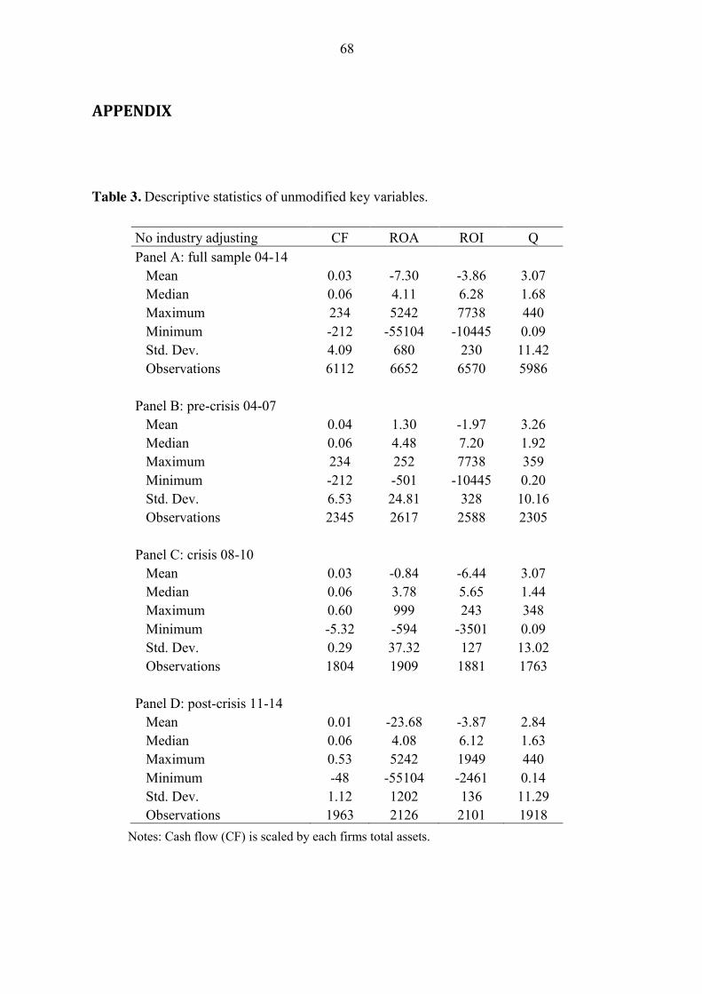
68

APPENDIX

Table 3. Descriptive statistics of unmodified key variables.

No industry adjusting CF ROA ROI Q Panel A: full sample 04-14 Mean 0.03 -7.30 -3.86 3.07 Median 0.06 4.11 6.28 1.68 Maximum 234 5242 7738 440 Minimum -212 -55104 -10445 0.09 Std. Dev. 4.09 680 230 11.42 Observations 6112 6652 6570 5986

Panel B: pre-crisis 04-07 Mean 0.04 1.30 -1.97 3.26

Median 0.06 4.48 7.20 1.92 Maximum 234 252 7738 359 Minimum -212 -501 -10445 0.20 Std. Dev. 6.53 24.81 328 10.16 Observations 2345 2617 2588 2305

Panel C: crisis 08-10 Mean 0.03 -0.84 -6.44 3.07

Median 0.06 3.78 5.65 1.44 Maximum 0.60 999 243 348 Minimum -5.32 -594 -3501 0.09 Std. Dev. 0.29 37.32 127 13.02 Observations 1804 1909 1881 1763

Panel D: post-crisis 11-14 Mean 0.01 -23.68 -3.87 2.84

Median 0.06 4.08 6.12 1.63 Maximum 0.53 5242 1949 440 Minimum -48 -55104 -2461 0.14 Std. Dev. 1.12 1202 136 11.29 Observations 1963 2126 2101 1918

Notes: Cash flow (CF) is scaled by each firms total assets.

69

Table 9. Empirical results of the full sample, without industry adjusting. Full sample 2004-2014 Lag t-1 Model 1 Model 2 Model 3 Model 4 Model 5 Model 6

Dependent variable: Capital expenditures/total assets.

Panel 9: independent variables.

Low CF -0.002* -0.007***

-0.001 -0.006** Medium CF

-0.005*** 0.002*

-0.005*** 0.001

High CF 0.005***

0.007*** 0.005***

0.006**

Low ROA -0.001 -0.003

-0.002 -0.007*** Medium ROA

-0.002 0.001

-0.005*** 0.002

High ROA 0.002

0.003 0.005***

0.007***

Low ROI -0.002 -0.004**

-0.004** -0.008*** Medium ROI

-0.002 0.001

-0.005*** 0.001

High ROI 0.002

0.002 0.005***

0.006***

Notes: *, **, *** = 10, 5 and 1% significance levels, respectively. Fixed cross-section and period effects and coef. covariance method = White cross-section. Tobin’s q is not presented here due to near zero impact on the dependent variable.