Embed Size (px)
Citation preview

Does income growth improve diet diversity in China?
Dung Doan
Crawford School of Public Policy
Australian National University
Selected Paper prepared for presentation at the 58th
AARES Annual Conference, Port Macquarie,
New South Wales, 4-7 February 2014
This paper has been independently reviewed and is published by the Australian Agricultural and
Resource Economics Society on the AgEcon Search website at http://ageconsearch.umn.edu/,
University of Minnesota, 1994 Buford Avenue, St Paul MN
Published 2014
Acknowledgements: I wish to acknowledge Prof. Bruce Chapman and Prof. Trevor Breusch for
their valuable guidance and extensive discussions throughout the process of this work. I am also
grateful to Dr. Annie Wei for her helpful advices on earlier versions of this paper. This research
uses data from the China Health and Nutrition Survey (CHNS). I thank the National Institute of
Nutrition and Food Safety, China Center for Disease Control and Prevention, and Carolina
Population Center, the University of North Carolina at Chapel Hill, for the CHNS data
collection.
Copyright 2014 by Dung Doan. All rights reserved. Readers may make verbatim copies of this
document for non-commercial purposes by any means, provided that this copyright notice
appears on all such copies.

Does income growth improve diet diversity in China?
Abstract
Recent studies on income and nutrition suggest that income growth plays either a small or even a
negative role in influencing diet quality in China, especially for low income households. Such
arguments cast doubt on the conventional reliance on income as a policy tool to improve public
health through better diets. They, however, have been drawn mostly from analysis of income
effect on nutrient intakes and diet adequacy. No research has been done on how income affects
diet diversity in China, despite its unambiguous health benefits. This paper tests if income
growth improves diet diversity, and, thus, can enhance public health in China, using data from
the China Health and Nutrition Survey 2004-2009. For the first time, potential endogeneity of
income, most likely due to omitted variables, is addressed in the estimation of income effect on
diet diversity by instrumental variables. This study finds that, regardless of estimation methods,
income effect is significant and positive, but diminishes along the income distribution and over
time. When endogeneity of income is controlled in 2SLS estimation, estimated income effect is
considerably larger than the corresponding OLS estimate. OLS regression shows that education
has significant and positive effects on diet diversity, with larger effects at higher education
levels. Nevertheless, education effects diminish in terms of both magnitude and statistical
significance in the 2SLS estimation. The stark differences between OLS and 2SLS estimates
suggest that it is important to account for endogeneity of income. The OLS estimation seemingly
understates income effects and overstates education effects. It, therefore, might mislead resource
allocation in designing food and health policies.
JEL code: I10, I15, D12, C12
Key words: nutrition, diet diversity, health economics, income, endogeneity

1
I. Introduction
Nutrition research has revealed a structural shift in food consumption patterns in developing
countries over the last few decades. Consumers have shifted away from diets of varying
nutritional qualities based on local grains, vegetables, and fruits toward diets higher in edible oil
and animal-source foods yet less diversified in nutrients and lower in fiber. This so-called
nutrition transition, or convergence to the ‘Western’ diet, is leading to significant increases in
non-communicable diseases and substantial changes in disease patterns of the population.
Obesity risks are shifting to the poor (Popkin 2004; Popkin & Gordon-Larsen 2004; Caballero
2005). Stroke, hypertension, and other diet-related chronic diseases are increasing in both
relative and absolute terms as causes of mortality and morbidity (Popkin et al. 2001, p.3).
Empirical evidence has also warned that increasing income does not necessarily improve diet
balance (Du et al. 2004) and adequacy (Banerjee & Duflo 2011), especially for low-income
people.
These warnings related to the detrimental health effects of changing diet as income rises
seemingly contradicts conventional food and nutrition policies. Resources allocated to alleviate
dietary problems, particularly through income-based programs or price subsidies, have often
been justified by the conventional wisdom that calorie and nutrient deficiencies are largely a
consequence of low income. If income growth in developing countries deteriorates diet quality
and adversely affects the population’s health, how should diet-related health issues be addressed?
The question of practical interest becomes, How much (if at all) increasing income enhances or
lowers diet quality, and consequently, public health? And is there any other policy instrument
that can improve diet quality? However, diet quality is a multi-dimensional, encompassing
adequacy, variety, moderation and overall balance of various nutrients. An answer to these
policy questions, thus, might depend on the aspect of diet quality being investigated.
An ample body of research on nutrition, health, and labor market outcomes has been devoted to
examining the relationship between income and diet adequacy. On the one hand, where hunger
and nutrient deficiencies are the most daunting dietary problems, assessing the income impact on
nutrient and/or food consumption quantity remains relevant and important. On the other hand,
the nutrition transition that many developing economies have been facing is characterized not by
a shortage of foods, but by a structural shift in patterns of food consumption. This requires that
the income-diet relationship is examined from angles other than diet adequacy. One prominent
candidate is diet diversity.
Economic studies on diversity of food consumption1, however, have been confined mostly in
explaining the demand for diversity by consumer theories. Little has been explored about what
income effects on diet variety mean in (i) understanding diet issues associated with income
growth and (ii) mitigating their adverse effects on health.
China presents a dynamic and academically attractive case of nutrition transition. Its rapid
economic growth in the last three decades has brought significant improvements in income and
living standard, as well as widening inequality across the country. Like many other emerging
1 In this paper, the terms diet variety, diet diversity, and food consumption diversity are used interchangeably.

2
economies, China has been experiencing the nutrition transition in the last two decades, and there
is evidence that the transition is accelerating. Some studies have found evidence that rising
income in China does not solve some key micronutrient deficiencies (Liu & Shankar 2007) but
increases consumption of high-fat low-fiber foods (Du et al. 2004, p. 1512). However, little has
been known about changes in diet diversity in this country. The sheer size of China’s population,
the pressing demand to maintain its economic competitiveness through higher labor quality, and
the neck-breaking pace in which things have been happening there requires a better
understanding of how much income determines changes in the structure and quality of the
Chinese diet.
Inspired by this gap in the literature, this paper tests the hypothesis that income growth improves
diet diversity, and, hence, can offset detrimental effects of the nutrition transition on health in
China during the period from 2004 to 2009. This study also explores the role of another key
policy instrument – education – in determining diet diversity. By investigating the effects of
these two instruments, this policy-oriented research will hopefully shed lights on how
government can influence diet diversity through income- and education-based programs. Using
data from the China Health and Nutrition Survey, the study constructs a measure of diet diversity
from the number of food groups consumed. It then addresses the potential issue of endogeneity
of income by two-stage least square (2SLS) estimation method.
The contribution of this study is threefold. First, it provides new insights into the changes in diet
quality as income rises in China. Proving positive and significant income effect on diet variety,
this study argues that net income effect on diet quality, and, consequently, net effect on health, is
not as negative as documented in the existing literature. This finding re-emphasizes the role of
income in improving diet-related utility and labor health. The paper also takes the literature one
step further by dissecting the analysis by region and shows that income effect is stronger in rural
areas.
Second, this is the first study that addresses the potential issue of endogeneity in the link between
income and diet variety by instrumental variables. To the best of the author’s knowledge,
potential endogeneity of income has been neglected by the existing empirical works on diet
diversity, though some research has taken into account the endogeneity of total calorie intake
(Drescher et al. 2009) and nutrition information (Variyam et al. 1998). This research argues that
the existence of income endogeneity might be qualitatively debatable. The Durbin-Wu-Hausman
test, however, detects its presence in the examined data. Estimates from OLS and 2SLS methods
show stark differences and indicate that OLS method might underestimate income effects while
overestimate education effect on diet diversity.
Third, this study has an advantage over the existing empirical studies in term of data quality. It
uses individual food consumption data, instead of household food expenditure, and, thus, avoids
aggregation errors of household level data in measuring individual consumption. The data
employed are also the most up-to-date nutritional data available for China. The nutrition
transition in China has been documented commencing as early as the early 1990s (Popkin et al.
2001). Yet the time frame of the empirical literature on changes in dietary consumption in China
has not reached beyond the year 2001. Rapid economic and demographic changes in this country
and evidence of inconstant income elasticities of nutrition consumption (Du et al. 2004)

3
discourage from making inference about the current situation from results of the 1990s. This
study attempts to bridge this gap by situating our analysis in the most recent period 2004-2009.
The remainder of this paper is organized as follows. Section 2 provides a critical review of
empirical research on income effects on dietary consumption behaviors, highlighting knowledge
gaps where this study hopes to fill in. Section 3 describes the data set and points out the
advantage of better data quality over existing empirical studies. Econometric models and
rationales for variables used in this study are presented in Section 4. Section 5 analyses
estimation results, and compares and contrasts them with existing evidence in the literature.
Section 6 concludes with some policy implications and suggestions for further research.
II. Literature review
The empirical studies on income as a determinant of dietary consumption can be broadly
categorized based on their dependent variables and how they analyze consumption. One
category, which is substantially more common, is devoted to explaining income effects on
consumption quantity of calorie, nutrients, and foods. The other investigates the role of income
on consumption patterns, including composition and relative share of different nutrients and
foods.
2.1 Income effects on dietary consumption – calorie, nutrient, and food
A conventional belief is that low energy and nutrient intakes are largely a consequence of low
income. However, the literature has not reached a conclusive agreement on the extent that
income drives calorie and nutrient consumptions. An overarching analysis by Strauss and
Thomas (1995) reviews 34 empirical papers and finds that estimated income elasticities of
calorie intake range from 0.01 to 1.18. They explain some of this wide range by methodological
differences. Estimated elasticities that are calculated indirectly from food demand equations tend
to be higher (ranging from 0.51 to 1.18) whereas direct estimates from calorie demand equations
tend to be considerably smaller (ranging from 0.56 to 0.01). An earlier study by Behrman and
Deolalikar (1987) had also made the same remark about the two approaches to estimate nutrient
elasticities with respect to household expenditure or income. The authors then argue that “the
direct estimates probably lead to better, though still possible upwardly biased, estimates” (p.
496).
Methodological differences, however, do not fully account for variations in income elasticity
estimates. Many studies have found a concave relationship between income and calorie
consumption, such as Pitt (1983), Chernichovsky and Meesook (1984), Garcia and Pinstrup-
Andersen (1987), Sahn (1988) and Ravallion (1990). Calorie elasticity with respect to income or
expenditure is found to be positive at low calorie intake levels and then flatten out at about 2,400
calories per capita per day (Strauss & Thomas, 1995, p.1903). Intuitively, calorie intakes are
likely to respond positively to income among the poor, but as income rises the elasticity will
decline, possibly to zero, or even become negative at high enough income levels.
More recent studies indeed find a negative association between income and calorie consumption,
i.e., as household income increases, people eat less. An example is Subramanian (2001), who

4
finds consumption of cereals, the cheapest and highest source of calorie, declines as income
increases in India. Banerjee and Duflo (2011) further argue that people do not always rationally
increase their food consumption as they have more money or as the real price of these foods fall.
The authors argue that even the money that people do spend on food is not spent to maximize the
intake of calorie or micronutrients. This article stresses that the poor or near poor might derive
utility from food and other non-food consumption differently from what standard economic
theories predict, and that many poor people are not hungry enough to seize every opportunity to
eat more.
The relationship between income and nutrient consumption is even more complicated. Various
researchers, such as Strauss and Thomas (1990), Subramanian and Deaton (1996), and again,
Banerjee and Duflo (2011), suggest that among poor urban households, when income rises,
getting more calories was not a priority, getting tastier foods was. The higher valued foods,
however, do not necessarily have higher nutrient content. Furthermore, income effects vary
across nutrients. For example, Skoufias et al. (2009) estimate income elasticity for various macro
and micro nutrients in rural Mexico and find mixed results. They obtain positive income
elasticities for fat, vitamin A and C, calcium, and iron, which have the largest deficiency in their
sample. Nonetheless, for the poorest households, “deficiency of total energy, protein, and zinc is
not accompanied by positive income elasticity” (p.657).
As we navigate the broad literature on income effects on dietary consumption, two important
points come to our attention. First, the widely varied estimates of income elasticities of calorie
and nutrient intakes caution against any generalization about both the direction and the
magnitude of income effects on household dietary consumption. The relationship might be either
positive or negative and the extent of income effect varies considerably across nutrients and
countries of interest. Second, examining dietary consumption at the nutrient level might not
suffice to inform about changes in diet quality, amidst the structural shift in consumption
patterns associated with income growth. Economic studies that aim to understand the role of
income in driving diet quality through changes in nutrient consumption, thus, have an intrinsic
shortcoming embedded in their dependent variables.
The majority of empirical studies on the causal link between income and dietary behaviours use
either the quantity of foods and/or nutrients consumed, or its log, or food expenditures as a
measure of the dietary consumption. Particularly, household per capita food expenditure has long
been employed to estimate income elasticities by authors such as Pitt (1983), Behrman &
Deolalikar (1987), and Sahn (1988). Another variable widely used in estimating responsiveness
of food consumption to household income and prices is log of food consumption. See, for
instance, Guo et al. (1999) and Du et al. (2004). At the nutrient level, log of calorie intake has
been used as the dependent variables in works by Ravallion (1990), Strauss & Thomas (1990),
Skoufias (2002), and Meng et al. (2007). Others have chosen to examine log of macronutrients,
namely fat, protein, and carbohydrate, and essential micronutrient intakes, such as iron and
vitamins. Examples of these studies include Liu & Shankar (2007), Mangyo (2008), and
Skoufias et al. (2009).
Using log of consumption quantity as the dependent variable is easy to interpret the estimated
coefficients. The coefficient of log of income then is simply the income elasticity of the food or

5
nutrient consumption. Similarly, elasticities of food expenditure with respect to income can be
easily drawn from demand equation using food expenditure as the dependent variable. These
conventional dietary variables remain important in studying how income or other policy
variables such as education and subsidies can improve social welfare through household meals,
especially in the context of subsistence economies where hunger and nutrient deficiencies are
serious issues.
Nutrient intakes, however, reveal limited information about diet quality and associated health
consequences. Higher level of calorie intake does not necessarily bring along higher health
benefit if the pre-existing level of calorie consumption is already adequate. As argued in
Skoufias et al. (2009), a significantly positive relationship between calorie and income does not
necessarily imply a higher consumption of essential nutrients since a higher income may simply
results in households buying more food with higher calorie density but low nutrient content, such
as instant foods and fast foods. In fact, marked shifts toward diets with higher energy density
have been documented in many developing countries. See, for example, Popkin et al. (2001) and
Popkin (2004). A similar argument applies when income elasticity for calorie is close to zero. As
household income falls, calorie consumption might be maintained through substitution between
and within food groups while the consumption of important nutrients may decrease drastically as
household consumes less meat, egg, vegetables and milk. Vitamin and micronutrient deficiency,
therefore, can exist as a condition independent of calorie adequacy (Subramanian 2001).
Moreover, a surplus of some nutrients such as fat and salt, through excessive consumption of
highly processed foods, can be even more harmful to health than a deficit of such nutrients.
Investigating consumption of calorie and individual nutrients, thus, provide only a partial
understanding about structural changes in diet quality and diet-related issues accompanying the
nutrition transition.
At the food level, how consumption responses to income changes depends on the food of
interest. Income is found to significantly decrease starchy foods and meat consumption, yet
increase milk consumption among Portuguese men (Moreira & Padrao 2004, p. 7). The same
study also finds that income changes do not affect consumption of vegetables, fruits, and fish. A
more recent paper by Ecker and Wain (2008) finds similar results in Malawi. The authors show
that income responsiveness is high for starchy foods, but relatively low for vegetables and fruits.
They observe the highest expenditure elasticities in animal-source foods and meal complements
such as cooking oil, sugar, and beverages (p. 22).
Changes in food consumption quantity reveal partly how composition of the diet evolves and
thus, partly fill the gap left by studies on nutrient intakes. Nevertheless, it is important to note
that more of a particular food group guarantees neither positive nor negative impact on health. It
depends on existing health and nutrition conditions of the individuals. It will be useful, hence, to
investigate a less ambiguous indicator of diet quality, more of which is synonymous with
beneficial impact on health.
2.2 Income effects on diet variety
Diet variety deserves attention for two reasons: well-grounded, unambiguous beneficial effect on
health and direct positive effect on utility. Amid the structural shift in diet patterns in developing
countries, diet diversity becomes even more relevant in indicating a healthy diet.

6
The variety of food consumption has been studied as one dimension of consumer demand for
diversity from both macroeconomics perspectives (such as trade, industrial organization) and
microeconomics perspectives (such as consumption behavior). Most relevant to this paper is
microeconomic theories explaining a preference for variety to an individual's consumption
behavior. As Weiss (2011) points out, we might distinguish two different approaches that explain
why consumers purchase a variety of products: “representative consumer models” and
“characteristics models” (p. 5). While “representative consumer models” derive a demand for
variety at the level of individual consumer, “characteristics models” typically explain it at the
market level. The traditional “representative consumer models” approach, which is more relevant
to the present study, views food diversity as a specific feature of the utility function. A
representative consumer maximizes his/her utility subject to a budget constraint. Differences in
the preference for variety are reflected in the curvature of the indifference curves and are
expressed in terms of the relative quantity of each product in the consumption basket (Weiss
2011, pp. 5-6).
It is beyond the scope of this study to review all those models in detail. But a notable model
often used as a theoretical background for empirical studies on food diversity is the hierarchic
demand systems suggested by Jackson (1984). Jackson introduces a hierarchy of purchase in
which only a subset of all goods available is actually consumed. Higher income allows additional
goods to enter the consumption bundle, forming a systematic relationship between income and
consumption diversity. As argued by Weiss (2011), however, theories often fall short in fully
explain consumer demand for variety due to various factors, often unobserved, that influence
consumption decisions. This is where empirical studies come into the picture. A brief summary
of relevant empirical works on income effect on diet diversity is presented in Table 1.

Table 1: Empirical studies that look at income effect on diet variety
Author Country Measure of diet
diversity
Food
grouping
Food
measurement
unit
Estimation
method Main findings
Drescher &
Goddard
(2011)
Canada Berry index 176 food
groups
food
expenditure
OLS and quantile
regression
Positive log-log relationship between income and diet variety. OLS
estimates: a 1% increase in real household annual income leads to
about 12.7% increase in the Berry index. Quantile regression shows
significantly different effects of independent variables across
quantiles. A 1% increase in income results in an increase of 8.3% to
24.6% in the Berry index. Education is not included in the regression
model.
Drescher et
al. (2009) Germany
Berry index;
Healthy Food
Diversity (HFD)
index
133 food
groups
no. of food
portions
OLS and 2SLS, IV
for total calorie
intake
Positive and significant linear income effect. An increase of 1000
Euro in household adult-equivalent monthly per capita income
results in an increase of 0.030 and 0.038 unit in the HFD and Berry
index, respectively. Positive education effect.
Drescher &
Goddard
(2008a)
Canada
Berry index;
count of food
items
176 food
groups
food
expenditure OLS
Significant concave quadratic relationship between income and food
diversity. At the sample mean, an increase of 1000 Canadian dollars
in annual household income per capita increases diet diversity by
0.115 food groups in 2001. Food prices, education and household
size are not included in estimation models.
Drescher &
Goddard
(2008b)
Canada
Canadian
Healthy Food
Diversity index
176 food
groups
food
expenditure OLS
Positive semi-log relationship between income and the Canadian HFD
index. Estimated coefficient of log of annual household income per
capita ranges from 0.015-0.046, depending on models and food
guides used. That is, when household income per capita doubles, the
index value increases by 0.015-0.046 units. Positive and increasing
education effect.
Theil & Weiss
(2003) Germany
Berry index;
Entropy index
149 food
groups,
excluding
fruit and
vegetables
food
expenditure OLS
Significant linear positive income effect. A 1000 DM increase in
household monthly income leads to an increase of 0.03 and 0.02
units in the Berry and Entropy index, respectively. Schooling of the
household's principle wage earner has almost insignificant effect.
Out of seven education levels, only the lowest and 3rd
lowest
education level had lower diversity as compared to the highest level.

8
Moon et al.
(2002) Bulgaria
Count of food
items; Entropy
index
102 food
items food weight
Negative binomial
II for count
measure, OLS for
Entropy index
Consumer preference for food variety exhibited difference patterns
depending on the length of time allowed for measuring
consumption. Positive and significant linear income and education
effects regardless of the length of time period allowed for
consumption and measure of diversity. Coefficients of household
income ranges from 0.019-0.041 for count measure. However,
factorial income and education variables were treated as continuous.
Hoddinott &
Yohannes
(2002)
10
developing
countries
Count of food
items
varies across
10 datasets food weight OLS
Diet diversity is positively associated with change in household per
capita consumption and household per capita caloric availability. The
results are independent of the methods used to estimation methods
nor of the methods used to collect the dietary data (24 hrs vs. 7-day
recall periods), although the magnitude of the impact differs. Approx.
0.65-1.11% change in household per capita consumption given a 1%
change in diet diversity.
Lee & Brown
(1989) USA
Berry index;
Entropy index
19 food
groups
food
expenditure OLS
Positive effect of total food expenditure and food stamp income on
diversity. Household expenditure was modeled in log form. Marginal
impact at the sample mean of 1 additional dollar of household
fortnightly food expenditure is 0.0021 and 0.0003 for entropy and
Berry, respectively.
Lee (1987) USA Count of food
items
153 food
groups food weight
OLS, Negative
binomial II,
Poisson
Positive linear income effect on diet diversity, regardless of
estimation method. One additional dollar of household weekly food
expenditure results in an increase of 0.0071, 0.0053, and 0.0074 food
groups consumed in the OLS, Poisson and negative binomial II
estimation, respectively.
Theil & Finke
(1983)
30
countries
Herfindahl
index; Entropy
index
various food
expenditure
Maximum
likelihood
estimation
Significant positive income effect. Elasticity of the Entropy index with
respect to real per capita income ranges from 0.058 in the richest
country (USA) to 0.441 in the poorest (India).

The empirical literature on food diversity has been consistent in proving positive income effects
on diet variety. In a multi-country analysis, Hoddinott and Yohannes (2002) use data from 10
developing countries and test whether household diet diversity was associated with household
per capita consumption, a proxy for household income, and household per capita calorie
availability. Their results show that on average a 1% increase in diet diversity results in a 1%
increase in per capita consumption. Another study by Moon et al. (2002) finds positive linear
income effect on diet diversity in Bulgaria, but magnitude varies depending on the reference
period that diversity is measured. The authors emphasize that the length of reference period
allowed for consumption is an important element in measuring the demand for food variety.
Studies in developed countries have also found similar results. Thiel and Weiss (2003), for
example, suggest that variety of German household food consumption linearly increases with
income. Demographic factors such as numbers of children, residential location, and employment
status of the housekeeping person are also significant in explaining diet diversity in their sample.
More recent works by Drescher and Goddard (2008, 2011) examine household diet diversity in
Canada and show evidences of a concave relationship between income and diet variety2.
These studies, however, were mainly motivated by a curiosity about consumer preferences and
decisions. Though some acknowledged health benefits of food diversity, diet diversity was often
analyzed as one dimension of consumer demand for diversity. Hardly any study has been
conducted with an explicit ex-ante focus on policy implication from diet diversity’s determinants
in light of the nutrition transition and its associated public health issues. A rare exception is
Drescher et al. (2009). Finding positive income and education effect, and significant roles of
behavioral variables, Drescher and colleagues explicitly suggest considering knowledge, age,
and willingness to pay for healthy food when promoting healthy eating.
Another shortcoming of the existing literature is their econometric estimation. Given diversity as
a feature of utility and the traditional diminishing marginal return, it is simplistic to assume a
linear correlation between income and diversity, as done in Moon et al. (2002), Thiel & Weiss
(2003), and Drescher (2009). (In fact, Moon et al. use categorical income data yet treat it as a
continuous variable in their regression analysis.) Drescher and Goddard (2011), though allowing
for non-linearity, fail to take into account education effect. Neither did the aforementioned
papers address potential inverse causality in the link between income and diet diversity.
2.3 Income effects on dietary consumption and diet quality in China
Empirical research on the income-diet relationship in China has been consistent with the broader
literature in terms of focusing on level of food and nutrient consumption. This body of research
has also examined the structural shift of food consumption patterns, such as changes in
consumption of animal-origin foods and grains. Among the most prominent studies on the
income-diet relationship in China are Guo et al. (2000) and Du et al. (2004). Estimating income
elasticities for a range of foods in China, Guo et al. (2000) conclude that income elasticities for
more luxurious foods increased significantly from 1989 to 1993, while less superior foods
became more inferior over this period. Similarly, Du et al. (2004) argue that important changes
2 Drescher and Goddard (2008a) suggest a concave quadratic relationship, while their more recent work in 2011
supports a semi-log relationship between income and diet diversity.

10
in income effects took place between 1989 and 1997, with the changes varying considerably by
income groups. The authors warn that “these shifts in income effects indicate that increased
income might have affected diets and body composition in a detrimental manner to health, with
those in low-income groups having the largest increase in harmful effects due to highest income
elasticities” (p. 1505).
At the nutrient level, Liu and Shankar (2007) model the determinants of the intakes of vitamin A
and D and test whether rising income will likely help overcome these two micro nutrition
deficiencies. Their results show a statistically significant but relatively small positive income
effect on both nutrient intakes. The local availability of milk is seen to have a strong positive
effect on intakes of both micronutrients. The paper then suggests that rather than relying on
increasing income, food policies like school milk programs might be more effective in stamping
out these vitamin deficiencies.
These results, together with other varying empirical results on the relationship between income
and nutrition intake, question the conventional reliance on rising income to improve diet-related
welfare in China. If rising income not only fails to improve diet quality, but might also
deteriorate it, income growth is likely to reverse or at least dampen the achievement in public
health thanks to hunger eradication. However, as discussed in earlier sub-section, the question of
how much (if any) rising income improves diet quality in China deserves to be examined with a
better and less ambiguous indicator of diet quality.
Moreover, to the best of the author’s knowledge, there is still no empirical literature investigating
the role of socioeconomic factors as a determinant of diet diversity in China. Evidences of a
positive association between income and diet diversity in other countries encourage this paper to
test if a relationship between income and diet variety exists in China, and if it does, what form it
takes. I will also take the literature one step further by dissecting the analysis by geographic
regions. This exercise will help determine if marginal effects of socioeconomic factors varies
across population subgroups.
III. Data and variables
3.1 Data
This study employs data at individual, household and community levels from the China Health
and Nutrition Surveys (CHNS). The survey is an on-going longitudinal collaborative work
between the Center of Population at the University of North Carolina at Chapel Hill and the
Institute of Nutrition and Food Safety, Chinese Center for Disease Control and Prevention. The
CHNS is one of the few datasets from developing countries that have information on individual
food consumption and nutrient intakes over time, making it particularly suitable for examining
the nutrition transition and household dietary behaviors.
The CHNS uses a multi-stage, randomized cluster design to survey approximately 3,800
households in nine provinces in China. The provinces are Guangxi, Guizhou, Heilongjiang,
Henan, Hubei, Hunan, Jiangsu, Liaoning, and Shandong. See Appendix 1 for a map of the
surveyed provinces. The survey’s sample, nevertheless, has no sampling weights and is not

11
representative at either province or national level. To control for multistage sampling and an
array of multilevel modeling issues, this paper utilizes various levels of control, as discussed in
more details in Section 3.2.
The sample is disaggregated into five administrative levels: (i) province, (ii) urban and rural, (iii)
city and county, (iv) urban/suburban and town/village, and (v) household. Counties and cities in
the provinces are stratified by income (low, middle, and high) and a weighted sampling was used
to randomly select four counties and two cities in each province. The provincial capital and a
lower income city were selected when feasible. Villages and townships within the counties and
urban and suburban neighborhoods within the cities were selected randomly. In each community,
20 households were randomly selected and all household members were surveyed. Since 2000,
the survey framework has contained 216 primary sampling units, consisting of 36 urban
neighborhoods, 36 suburban neighborhoods, 36 towns, and 108 villages.
The dataset used in this paper is taken from three waves of the CHNS: 2004, 2006, and 2009.
With a strong focus on the labor force, this paper limits the sample to 11,146 adults (18-60 years
old) from 4,506 households, among which 3,891 individuals were interviewed in all three waves.
After accounting for missing data, the actual regression sample size for the 3 years is 5,182,
4,971, and 5,010 observations, respectively. Geographical distribution of the sample is displayed
in Figures 1 and 2.
Figure 1: Rural-urban distribution of dataset
34% 34% 33%39% 38% 40%
66% 66% 67%61% 62% 60%
0%
10%
20%
30%
40%
50%
60%
70%
80%
90%
100%
2004 2006 2009 2004 2006 2009
Rural
Urban
Survey sample Regression sample

12
Figure 2: Geographical distribution of dataset
The detailed records of individual food consumption from the CHNS provide this paper an
advantage over studies using household level data. Household food expenditure or food
consumption data neglect the intra-household distribution of food and thus, impose aggregation
errors in measuring individual consumption (Ecker & Wain 2008, p. 14). Besides, nutrient
requirements and recommendations are defined for individuals of particular gender and age.
Nutritional implication from household level data, thus, must be applied with caution to any
specific demographic population groups by age or gender, which in many cases is of special
interest.
0%
10%
20%
30%
40%
50%
60%
70%
80%
90%
100%
2004 2006 2009
Survey sample
Guizhou
Guangxi
Hunan
Hubei
Henan
Shandong
Jiangsu
Heilongjiang
Liaoning
0%
10%
20%
30%
40%
50%
60%
70%
80%
90%
100%
2004 2006 2009
Regression sample
Guizhou
Guangxi
Hunan
Hubei
Henan
Shandong
Jiangsu
Heilongjiang
Liaoning

13
3.2 Variables
3.2.1 Dependent variables
As mentioned in earlier sections, this paper investigates the relationship between income and diet
quality in China from the angle of diet diversity. Two major reasons justify the usage of diet
diversity as an indicator of diet quality. First, the essential role of diet variety in maintaining
good health is well-grounded and unambiguous in both the nutrition literature (Ruel 2002) and
governmental nutrition policies. Improving the variety of food consumption across and within
food groups is the first recommendation in most official dietary guidelines, including the Dietary
Guidelines for Australian Adults (NHMRC 2003), Dietary Guidelines for Americans (USDA &
USDHHS 2010), Dietary Guidelines for Chinese Residents 2007 and the Chinese Food Guide
Pagoda 2007 (Ge 2011). Measures of diet variety have also been used as a component in various
diet quality scores, such as the DQI Revised by Haines et al. (1999), INFH-UNC-CH DQI by
Stookey et al. (2000), and DQI - International by Kim et al. (2003). Second, nutrition studies in
developing countries have validated a positive relationship between dietary variety and nutrient
adequacy3. Thus, diet variety is not only an informative indicator of diet quality, but could also
be “a useful indicator of household food security” (Ruel 2002, p. iii; Ruel 2003).
Having justified the usage of diet variety as a dependent variable based on its health benefits, this
paper closely follows the nutrition literature in measuring diet variety. Diet diversity is often
measured using a simple count of foods or food groups over a reference period, but several foods
grouping and classification systems have been used (Ruel 2002). To generate a measure of diet
variety applicable to the Chinese diet, this study follows the Diet Quality Index – International
developed by Kim et al. (2003) and constructs our variety variable as follows. A well-diversified
diet should consist of foods from all 5 broad food groups: grain, meat, vegetable, fruits, and
diary. Although individual food items can be categorized according to different degrees of
aggregation, these 5 broad food groups capture the main sources of important nutrients required
for a healthy body.
The dietary section of the CHNS records individual’s food intake on a 24-hour-recall basis for
three consecutive days for each survey year. Food items are assigned into one of the five selected
broad food groups based on the classification in the Chinese Food Composition Table (Yang et
al. 2004, 2009). Diet variety then is measured as the average daily number of food groups
consumed by an individual. Following Stookey et al. (2000), a food group is counted if its daily
consumption quantity is larger than 25 grams. This amount is deemed to be nutritionally
meaningful. Our diet variety variable is, thus, on a range from 1 to 5.
3 Ruel (2003) provides a careful review of studies that validate diet diversity against nutrient adequacy, child
nutritional status and growth.

14
Table 2: Distribution of dependent variable
Count of food groups consumed 2004 2006 2009
Frequency
1 2 2 1
2 502 316 174
3 1,753 1,573 1,253
4 2,298 2,241 2,352
5 627 838 1,230
Total 5,182 4,971 5,010
Mean 3.52 3.68 3.85
Std. Dev. 0.81 0.81 0.79
As can be seen in Table 3, diet diversity is relatively concentrated around its mean and increases
over time. Though the concentration of the variable might raise some concerns, the regression
results presented in later sections suggest that the data have enough variation to generate
significant estimated relationships.
It should be noted that alternative measures have been used in the economics literature. Popular
alternatives include the Berry index (or the Simpson index) (Berry 1971; Lee & Brown 1989;
Drescher & Goddard 2008, 2011; Theil & Weiss 2003), the Entropy index (Lee & Brown 1989;
Moon et al. 2002; Theil & Weiss 2003), and the Healthy Food Diversity Index (Drescher et al.
2007, 2009). A less popular measure is the Hirschman-Herfindahl index, used by Theil and
Finke (1983). These measures take into account the relative share of each food group consumed
within the total food consumption, while a count measure does not.
Despite this advantage, they are ruled out for two reasons. First, their values are difficult to
interpret in absolute terms. This imposes a challenge for policy making when we are concerned
about policy implication from estimated effects of policy instruments like income and education.
Second, the more popular Berry index and Entropy index only measure the degree of
consumption diversity but does not reflect health benefits of diet diversity. These two indexes are
higher when a larger number of foods are eaten in equal shares. From a nutritional perspective,
nonetheless, foods should be consumed according to recommended quantities and relative
shares, not in equal share. In this sense, these indexes are not better than a count measure in
terms of capturing health aspects of a diversified diet.
Probably the only diversity measure that attempts to incorporate the health value of a food basket
is the Healthy Food Diversity index proposed by Drescher et al. (2007). Building on the Berry
index, the authors introduced a health factor for each food group based on the food pyramid of
the German Nutrition Society. This pyramid, unfortunately, is hardly applicable to the Chinese
diet. It illustrates dietary recommendations for the German population, which has very different
cuisines, food availability, and biophysical conditions from its Chinese counterpart. Moreover,
the health factors are calculated by multiplying the quantitative and qualitative dimensions of the
recommended foods. These “graphically depicted qualitative dimensions” in the pyramid are
quantified by assigning a percentage value to each food group (Drescher et al. 2009, p. 686). In a
later study, the authors note that such “explicit valuation of foods is an own interpretation of the

15
German Food guidelines” (Drescher et al. 2009, p. 686). The health factors used to calculate the
Healthy Food Diversity index, thus, may be ad-hoc.
3.2.2 Independent variables
A key explanatory variable in our study is real annual household income per capita, inflated to
2009 price. Household income per capita has been adjusted for the adult equivalence scale to
account for differences in consumption of household resources by members of different ages.
This paper employs the modified OECD adult equivalent scale. The first adult in a household is
counted as 1, each of the other adults as 0.7, and each of the children younger than 18 years old
as 0.5. Summary statistics of household income in Table 4 show considerable inequality across
provinces. Mean income of the poorest one is about 50%, 46%, and 55% of that of the richest in
2004, 2006, and 2009, respectively. Although income rise is rapid by international standard in all
provinces, the specific growth rate varies. The highest annual accumulated rate between 2004
and 2009 is observed in Hubei (16.4%) and lowest in Jiangsu (4.8%).
Other explanatory variables likely to affect food consumption include community- and
household-specific characteristics as well as individual demographic information. At the
community level, province dummy and rural dummy variables are modeled in order to control
for differences in dietary tradition, general lifestyle, and food availability across regions.
Potential price effects are taken into account by controlling for food prices at community level.
The model includes prices of rice, pork, fish, cabbage, tofu, apple, and soy oil, as representatives
of grain, meat, vegetables, bean products, fruits, and edible oils, respectively. All price variables
are in log form and measured in Yuan.
A household-specific characteristic that might influence food consumption is household size.
Again, this variable is adjusted to the modified OECD adult equivalent scale. Adjusted
household size is then the adjusted number of household members.
Education is conventionally modeled in demand equations as an indicator of knowledge and,
thus, is expected to affect consumer’s behaviors. In the context of this study, education of an
individual is expected to determine his/her food consumption decisions. In order to allow for a
flexible relationship between education and diet variety, the highest level of education attainment
is categorized into 6 groups: no formal education, primary school, secondary school, high school,
vocational training, and university and higher. This ordered factorial variable will be able to
capture impact of having a higher level of education on diet variety, without imposing a rigid and
possibly controversial relationship between years of schooling and the dependent variable.
Other relevant individual demographic variables4 include age, gender, and daily average food
consumption, measured in kilograms. The daily average quantity of food consumed will help
control for the changes in number of food items consumed as quantity of food intake changes.
Occupation, though, might reflect variation in lifestyle and dietary habits, is highly correlated
with education and at least partly with household income, and thus, is not included in this model.
Summary statistics for all explanatory variables are shown in Table 4.
4 Since more than 88% of our sample belongs to the Han ethnic group, leading to little contrast in the data, we do
not include ethnicity in our model.

16
Table 3: Summary statistics of independent variables
Variables 2004 2006 2009
Mean Std. Dev. Mean Std. Dev. Mean Std. Dev.
Age 42.00 10.77 42.87 10.68 43.31 11.02
Gender (% of female) 52.1%
52.3%
52.2%
Household size 3.47 1.25 3.58 1.38 3.48 1.35
Education
Years of schooling 8.68 3.90 8.64 4.23 9.02 4.05
No education 11.2%
15.4%
12.6%
Primary school 21.6%
17.5%
15.5%
Secondary school 36.7%
35.8%
39.3%
High school 17.2%
16.6%
16.5%
Vocational training 8.2%
7.9%
8.8%
University and higher 5.1%
6.9%
7.3%
Real annual household adult-equivalent per capita income(2009 Yuan)
Overall 10,033 9,547 11,436 16,396 16,215 21,658
Liaoning 10,837 10,287 12,712 11,864 16,245 17,633
Heilongjiang 10,261 9,274 12,029 14,338 16,750 19,680
Jiangsu 15,880 12,037 14,244 14,681 19,610 17,695
Shandong 8,617 7,852 13,315 27,232 17,106 23,641
Henan 6,720 6,136 9,126 11,458 12,568 15,555
Hubei 7,854 8,017 11,386 25,796 14,983 22,393
Hunan 10,252 9,534 11,758 14,862 17,596 32,049
Guangxi 8,546 7,169 7,184 5,564 13,155 17,567
Guizhou 8,521 8,706 9,785 11,047 16,459 19,249
Prices (Yuan per kg / liter)
Rice 1.27 0.21 1.38 0.23 1.66 0.68
Pork 7.12 1.27 5.93 1.15 9.18 1.43
Fish 4.77 4.13 4.10 0.96 5.08 1.40
Cabbage 0.67 2.45 0.83 1.42 1.01 0.83
Tofu 2.53 1.52 2.28 1.04 3.33 1.49
Apple 1.37 0.73 1.88 0.76 2.44 0.90
Soy oil 4.09 1.41 3.81 1.30 5.04 1.90
17
IV. OLS models and estimated results
4.1 OLS models
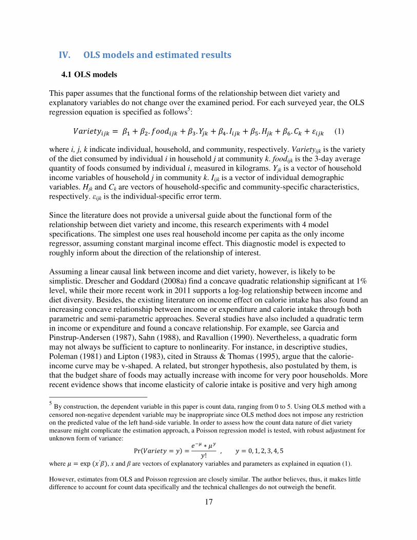
This paper assumes that the functional forms of the relationship between diet variety and
explanatory variables do not change over the examined period. For each surveyed year, the OLS
regression equation is specified as follows5:
�������� � � � �. ����� � �. � � �. �� � �. � � �. � � �� (1)
where i, j, k indicate individual, household, and community, respectively. Varietyijk is the variety
of the diet consumed by individual i in household j at community k. foodijk is the 3-day average
quantity of foods consumed by individual i, measured in kilograms. Yjk is a vector of household
income variables of household j in community k. Iijk is a vector of individual demographic
variables. Hjk and Ck are vectors of household-specific and community-specific characteristics,
respectively. εijk is the individual-specific error term.
Since the literature does not provide a universal guide about the functional form of the
relationship between diet variety and income, this research experiments with 4 model
specifications. The simplest one uses real household income per capita as the only income
regressor, assuming constant marginal income effect. This diagnostic model is expected to
roughly inform about the direction of the relationship of interest.
Assuming a linear causal link between income and diet variety, however, is likely to be
simplistic. Drescher and Goddard (2008a) find a concave quadratic relationship significant at 1%
level, while their more recent work in 2011 supports a log-log relationship between income and
diet diversity. Besides, the existing literature on income effect on calorie intake has also found an
increasing concave relationship between income or expenditure and calorie intake through both
parametric and semi-parametric approaches. Several studies have also included a quadratic term
in income or expenditure and found a concave relationship. For example, see Garcia and
Pinstrup-Andersen (1987), Sahn (1988), and Ravallion (1990). Nevertheless, a quadratic form
may not always be sufficient to capture to nonlinearity. For instance, in descriptive studies,
Poleman (1981) and Lipton (1983), cited in Strauss & Thomas (1995), argue that the calorie-
income curve may be v-shaped. A related, but stronger hypothesis, also postulated by them, is
that the budget share of foods may actually increase with income for very poor households. More
recent evidence shows that income elasticity of calorie intake is positive and very high among
5 By construction, the dependent variable in this paper is count data, ranging from 0 to 5. Using OLS method with a
censored non-negative dependent variable may be inappropriate since OLS method does not impose any restriction
on the predicted value of the left hand-side variable. In order to assess how the count data nature of diet variety
measure might complicate the estimation approach, a Poisson regression model is tested, with robust adjustment for
unknown form of variance:
Pr ������� � �! � �"# $ %&
�! , � � 0, 1, 2, 3, 4, 5
where % � exp 2 ′ !, x and β are vectors of explanatory variables and parameters as explained in equation (1).
However, estimates from OLS and Poisson regression are closely similar. The author believes, thus, it makes little
difference to account for count data specifically and the technical challenges do not outweigh the benefit.

18
poor households, but the curve flats out when calorie consumption reaches about 2400 kcal/day
(Strauss & Thomas, 1995). These empirical findings hint that the present relationship between
diet diversity and income might display similar nonlinearity.
These possibilities are tested by models 2 and 3. The second and third specifications model
quadratic and semi-log relationship between income and diet variety, respectively. Of course,
quadratic and semi-log are only basic ways of dealing with nonlinearity. The last specification
uses income quintiles to avoid imposing a rigid function of nonlinearity yet still allow for
variation in income effects across income groups.
Statistical software STATA, version 11.0, is used to clean the datasets and implement all
analyses. The empirical analysis begins by formally testing the presence of heteroskedasticity by
the Breusch-Pagan test across all years and model specifications. The test statistics strongly
reject the presence of constant variance of the error term and hence, justify the employment of
the robust option in estimating coefficient variance.
4.2 OLS estimates: Income effects
OLS estimated coefficients of real household income per capita are presented in Table 1 for all
four model specifications. For brevity, the full set of OLS estimated results is provided in
Appendix 2. Standard errors in this appendix and elsewhere in this paper are all robust to
heteroskedasticity.
Table 4: OLS estimated coefficients of real household income per capita
Model Variable 2004 2006 2009
1 Income 0.078*** 0.013* 0.009**
2 Income 0.189*** 0.083*** 0.031***
Income squared -0.022*** -0.005*** -0.001***
3 Log of income 0.090*** 0.067*** 0.039***
4
Quintile 2 0.092*** 0.103*** 0.036
Quintile 3 0.157*** 0.191*** 0.062*
Quintile 4 0.237*** 0.253*** 0.045
Quintile 5 0.307*** 0.274*** 0.151***
* p < 0.10, ** p < 0.05, *** p < 0.01
The “diagnostic” model 1 suggests that household per capita income has a positive, yet
decreasing impact on diet variety over the examined period. The estimated coefficients of
income decline in terms of both magnitude and statistical significance over time.
Model 2 reveals a concave quadratic relationship significant at 1% level between diet variety and
income. This result dictates that as income increases, diet variety will be improved at a
diminishing rate until it reaches a maximal point, from which onwards, diet variety will fall.
However, holding all other explanatory variables in the model constant, the maximal point of
diet variety is achieved at an annual household income per capita of 42.6, 91.2, and 138.6

19
thousands Yuan in 2004, 2006, and 2009, respectively. These optimal levels of income are well
above the mean income of the richest quintile in their respective years. Only 3.05, 2.64, and
2.30% of the regression sample have income higher than these optional values in the three
respective years. In other words, income of the majority of examined sample is still low enough
to guarantee an improvement in diet variety as it rises. Although the exact magnitude of
income’s marginal effect depends on the level of household income, this finding supports our
intuitive expectation that higher earnings allows for a broader consumption basket, and thus, a
more diversified diet.
The exceptionally high values of optimal income levels, relative to most of the income
distribution, also raise a caution. The concave quadratic relationship, though statistically
significant, might be due to some outliers that have extremely high income yet relatively lower
diet variety than those with lower income and similar non-income characteristics. These few
observations give grounds for suspecting that the true relationship between income and diet
variety might be positive and concave, but not necessarily quadratic. This suspicion is further
enforced by previous empirical works. As discussed in the previous section, the literature has
suggested that a quadratic form may not always be sufficient to capture nonlinearity in income
effects.
Turning to the hypothesis of a semi-log relationship between income and diet diversity, this
study finds that income effect flattens in 2009. The coefficient of log of income is simply the
marginal change in diet variety as income doubles. In 2004, when annual household income per
head is doubled, diet variety increases by approximately 0.09 food groups. The figure drops to
0.04 food groups in 2009. This pattern of decreasing income effect seems to follow the same line
of findings in models 1 and 2.
Comparison between the quadratic and semi-log specifications is made by calculating marginal
income effect at different points along the income distribution. Figure 3 below presents the
estimated marginal change in diet variety as real household income per capita rises by 1000
Yuans (approximately USD146). The marginal effect is computed at six different points: the
sample mean and the mean of each income quintile. On average, the estimated marginal effect at
the sample mean is higher in the quadratic model. The semi-log model yields a steeper slope at
the lowest income quintile, yet flats out faster as income increases.

20
Figure 3: Estimated marginal impact of 1000 additional Yuan at mean income
Differences in categorizing food items and measuring diversity make it hard to compare
magnitude of the present estimated coefficients with existing evidences. Nevertheless, all three
models above produce consistent estimates with those of earlier studies in terms of sign and
statistical significance, namely a positive linear income effect found by Moon et al. (2002), Theil
and Weiss (2003), and Drescher et al. (2009), a concave quadratic income-diversity relationship
in Drescher and Goddard (2008), and a log-log relationship in Drescher and Goddard (2011). See
Table 6 below for a rough comparison of this research and existing empirical results. A more
detailed summary of these studies is displayed in Table 1.
More importantly, the tested non-linear relationships both suggest that diet variety of low-
income people is more responsive to income changes than that of the rich. Income programs,
thus, provide a straightforward channel to promote healthy eating among this vulnerable group.
Table 5: Comparison of OLS estimated income effect with existing empirical results
Model Relationship Estimated marginal impact of 1000 additional Yuans/Dollars/Euros
This study Existing studies
1 Linear 0.0014- 0.0085 food
groups
• 0.019-0.041 food groups (Moon et al. 2002) – income
measured as a factorial variable, food group ranges f
• 0.02-0.03 units of Berry and Entropy index, respectively (Theil
& Weiss 2003) – income measured in Deutsche Mark
• 0.030-0.038 units of HFD index (Drescher et al. 2009) – income
measured in Euro
2 Quadratic 0.0039-0.0104 food
groups
• 0.080-0.138 food groups – income measured in Canadian
dollar (Drescher & Goddard 2008a)
0.00
0.01
0.02
0.03
0.04
0.05
0.06
0.07
Sample mean Quintile 1 Quintile 2 Quintile 3 Quintile 4 Quintile 5
2004_quadratic 2006_quadratic 2009_quadratic
2004_semi log 2006_semi log 2009_semi log

21
3 Semi-log 0.0015-0.0055 food
groups
• 0.0013-0.0014 units of Canadian HFD index (Drescher &
Goddard 2008b) – income measured in Canadian dollar
Releasing the rigid functional forms above, model 4 estimates impact of being in the second,
third, fourth, and fifth quintile relative to being in the poorest one. Its results, shown in the last
panel of Table 5, corroborate that there is a positive link between income and diet variety, yet
income effects vary across income groups. Compared to the poorest 20% of the sample, the diet
of the richer quintiles contains approximately 0.1 to 0.3 more food groups in 2004 and 2006. The
relative differences among the quintiles, however, seem to narrow over time. In 2009, only the
richest quintile has a better diet in terms of variety than the base quintile, tested at 1% level.
Again, this proves a diminishing role of income in influencing diet diversity over time.
Going beyond analysis within each survey year, we are particularly interested in how the income
effect evolves across the three cross sections. As shown in Table 5 and Figure 3, despite their
different functional forms, all models show that estimated income coefficients fall over the
examined period.
Two important points arise as we focus on the decrease in marginal income effects over time.
First, these changes can be partly explained by the underlying income growth. Ceteris paribus, a
higher income level in a later year indicates a shift to the right along the relationship function,
i.e. to the flatter portion of the curve. Thus, even if the relationship remains unchanged over
time, income growth leads to lower income marginal effect on diet variety. The relative changes
in income effects are consistent with the income growth rates of the two periods 2004-2006 and
2006-2009. Income marginal impact drops relatively less during 2004-2006 than during 2006-
2009. This is matched by a lower growth rate of mean household income per capita during the
earlier period (8.6% per annum) as compared to 11.9% in the later. Second, the slope of the
estimated relationship declines, causing lower marginal income effects over the examined
period. A possible explanation for this lies in the nature of the data. Assume the true relationship
is concave and remains constant over time. The observed sample, however, move towards the
right tail of the income distribution. In other words, the sample contains more observations on
the flatter section of the true relationship. Linear estimation, which is based on the observed data,
then detects flatter slope and yields smaller estimated coefficients.
To compare the above specifications, model selection criteria AIC and BIC are employed. As
can be seen in Appendix 2, the semi-log model (model 3) yields the lowest AIC and BIC values,
and thus, should be preferred among the tested specifications. Henceforth, we will interpret
estimated coefficients of the remaining explanatory variables from this model

22
4.3 OLS estimates: Education effects
Table 6: OLS estimated coefficients of education
Education level 2004 2006 2009
Primary 0.122*** 0.026 0.113***
Secondary 0.258*** 0.192*** 0.165***
High school 0.398*** 0.300*** 0.255***
Vocational training 0.587*** 0.492*** 0.387***
University & above 0.572*** 0.398*** 0.405***
* p < 0.10, ** p < 0.05, *** p < 0.01
Table 8 displays estimates of coefficients of five education levels from model 3, as compared to
the base group (no education). Except individuals with only primary school education in 2006,
formally educated consumers consistently have higher diet diversity than the base group, who
had no formal schooling, across the three examined years. Generally, the higher the education
attainment, the larger the difference in diet diversity as compared to the base group. Although the
estimated coefficient for vocational training is slightly higher than that for university education
in 2004 and 2006, they are not significantly different from each other even at 10% level (F
statistics=0.10, p-value=0.76). This monotonic pattern of positive and increasing impacts of
education on diet variety is not surprising. Better educated people are likely to be more
knowledgeable and/or more concerned about health and nutritional balance. So on average, they
make better informed food consumption decisions. The positive role of education and knowledge
in influencing food choices has also been detected earlier in OLS estimation by Variyam et al.
(1998), Moon et al. (2002), and Drescher et al. (2009), among others.
Interestingly, the coefficients of education attainments appear to fall over time. Keep in mind
that these are the relative differences in diet variety between individuals with some education and
the base group. These narrowing gaps between formally educated and uneducated consumers
suggests that education might no longer as effective in improving diet diversity in 2006 and 2009
as it used to be in 2004. Probably more available information or changes in life style make diet
of people with formal education not much more diversified than that of the base group as it used
to be. Still, vocational training and tertiary education remain important in supporting healthy
food consumption. A university graduate or vocational training graduate on average consumes
about 0.4 more food groups per day than an individual without any education. That difference is
about half of the standard deviation of diet diversity in each surveyed year.
4.4 OLS estimates: Effects of community factors
Given the vast geographical coverage of the sample, we expect local fixed effects to play an
important role in shaping how diversified the diet is. Liaoning is used as the base province. As
shown in Table 8 below, individuals from all provinces, except Jiangsu, consistently have lower
diet diversity than their counterparts in Liaoning, tested at 1% level.

23
Table 7: OLS estimated coefficients of community factors
Community variables 2004 2006 2009
Province
Heilongjiang -0.481*** -0.251*** -0.457***
Jiangsu -0.054 -0.082* -0.507***
Shandong -0.159*** -0.355*** -0.295***
Henan -0.399*** -0.568*** -0.672***
Hubei -0.379*** -0.604*** -0.727***
Hunan -0.289*** -0.254*** -0.633***
Guangxi -0.577*** -0.667*** -0.569***
Guizhou -0.253*** -0.233*** -0.558***
Rural -0.356*** -0.195*** -0.251***
* p < 0.10, ** p < 0.05, *** p < 0.01
Judging from the magnitude of the estimates of the provincial dummies, the relative differences
among the estimates appear to follow neither the income variation across the provinces nor their
geographical neighborhood. For example, Heilongjiang had significantly lower diet diversity
than the omitted province, which had similar a mean income level in all 3 years. Similarly,
Hubei’s mean annual income in 2006 is 11,386 Yuan per capita, very similar to its neighbour
Hunan (11,758 Yuan); yet the coefficient for Hubei is more similar to that for Guangxi, the
poorest province of the year (7,186 Yuan per capita). The two neighboring coastal provinces
Shandong and Jiangsu do not seem similar, either.
This observation suggests that the provincial dummies are likely to have captured impacts of
non-income factors among the surveyed provinces. Those factors could be anything, but mostly
unobserved, such as: culture and lifestyle, taste, food availability, cuisine, weather, etc.
Individuals living in rural areas have a less diversified diet on average than their urban
counterparts. This could be attributed to a narrower range of foods available in rural areas. Food
choice of rural residents might be constrained by the foods produced locally and/or shortage of
non-traditional food such as milk and dairy products, which makes their diet less diversified.
V. 2SLS models and estimated results
5.1 2SLS models
An important issue which needs to be addressed, yet has been neglected by the literature, in
modeling the relationship between diet variety and income is potential endogeneity. The causal
link between income and diet diversity might be mutual. Diet variety, by promoting good health,
could positively affect labor income through higher labor supply and/or higher productivity. On
the other hand, higher income allows for a larger consumption basket and thus, might have a
positive impact on diet variety. In this case, the OLS estimated income effect will be biased
upward and the bias may be higher for low income earners.

24
Similar concerns about endogeneity of income have played a prominent role in the literature
about income effect on nutrient intakes. Current nutrient intakes might raise labor supply and/or
productivity, especially for jobs that require heavy physical effort. In a comprehensive review of
this literature, Strauss and Thomas (1995) state that ‘… as well as endogeneity of income or
expenditure, and the validity of instruments are all very important concerns’ (p.1901). The same
research also discusses the reverse relationship between nutrients and, more generally health, on
income. The authors then stress that ‘correlation between any component of income (such as
wages or labor supply) and measure of health that depend on current behavior could reflect
causality in either direction’ (p. 1911). Empirical studies on the responsiveness of nutrient
intakes to income have also paid special attention to controlling for inverse causality. Example
includes Berhman and Deolalikar (1987), Bouis and Haddad (1992), and Skoufias et al. (2009).
If we believe in such inverse causality, the same logic could be applied to the correlation
between income and diet diversity. In the context of this study, however, the presence of
simultaneity is debatable. Diet variety, through nutrition effect on labor supply and productivity,
may take a considerable time before it can influence income, while current income is very likely
to directly impact current diet. Besides, if a household member does not contribute to the
household’s income through his/her labor supply, her dietary changes will have no effect on
household income per capita. So if past and current diet varieties are not correlated, simultaneity
is not present in equation (1).
Over and above concerns with simultaneity, endogeneity in this study is more likely to arise from
omitted variables. Many unobserved factors could influence food choices and diet variety, such
as taste, physical activity level, health condition, and consumer’s perception about the social
image that their foods project. For example, rich people might prefer to consume more expensive
foods to prove their social status. It is also possible that taste for work and lifestyle is correlated
with taste for food consumption. People with a strong preference for a lavish lifestyle might be
more motivated to work harder and earn higher incomes. They may also have a jaded palate and
choose to consume a more restrictive range of foods. However, the sign of the omitted variable
bias in this case is not clear. It depends on (i) the sign of the coefficient of the omitted variable in
the true model, and (ii) the correlation between the omitted variable and the remaining variables
in the estimated model6.
Assuming the absence of mutual causality, the OLS estimated income effect is conditional on
only observed variables included in the model. That estimate captures both the “true” income
effect, which influences diet diversity solely through higher purchasing power, and indirect
effects through income of omitted factors that correlate with income. In this sense, the “true”
income effect is the effect often expected from income-based policies, such as cash transfer
schemes or food coupons. Such programs effectively increase the disposable income of the
6 Wooldridge (2006) provides a useful discussion on the omitted variable bias in two simple cases, where the
estimated model has only one and two regressors, respectively (pp. 95-99). Suppose the true model is
� � 3�. 2� � 3�. 2� � 4� 3"�. 2"� � 3 . 2 � � 3!
yet the estimated model omit xk :
� � 5�. 2� � 5�. 2� � 4� 5"�. 2"� � 6 4!
It is easy to see that 78 � 79 � 3. :� where γi is the estimated coefficient of xi in the auxiliary regression of xk on x1,
x2, … xk-1. The omitted variable bias will be 3 . :� (i=1, 2, …, k-1)

25
targeted population, while keeping all other factors constant. From a policy maker’s point of
view, therefore, it is more important to know the marginal effect of income that is conditional on
both observed and unobserved variables. The OLS estimates, unfortunately, fails to distinguish
the “true” income effect and the indirect effect of unobserved variables.
In the presence of endogeneity, OLS estimator of equation (1) will be inconsistent and biased.
Thus, even though the existence of endogeneity of income is controversial, it deserves to be
addressed. As far as the author knows, this study is the first to do so by using instruments for
household income and estimate equation (1) by 2SLS method. The existence of endogeneity will
be formally tested. Estimates from OLS and 2SLS methods will be compared in later sections.
The choice of a valid instrument is always a complicated task. Ideally, we want an instrumental
variable that is correlated with household income per capita but not with diet variety or
unobserved factors that influence diet variety. The literature on income effects on dietary intakes
has used a wide variety of instruments for household income or expenditure. Examples include
but are not limited to non-labor income, factors associated with permanent income such as farm
size, schooling of household head (Behrman & Deolalikar 1987), non-food expenditure and
count of household assets (Skoufias et al. 2009), and rainfall (Behrman & Deolalikar 1987;
Mangyo 2008).
Given the available data in the CHNS, this study uses count of household durable assets and tries
3 different sets of instruments for household income per capita. The first set (IV1) is only the
total number of durable assets owned by the household. The second one (IV2) includes the
numbers of car, color TV, fan, and computer, individually. The third set (IV3) consists of the
numbers of car, microwave, and camera7, individually. The stock of durables is effectively a
measure of wealth and is informative about household income. In a static model current
productivity and/or labor supply should be unaffected by wealth, so it may be a valid instrument
(Strauss & Thomas 1995). A priori this study assumes that the only possible link between stock
of durables and diet variety is through income, i.e. there is no causal relationship between
number of durable assets and how diversified household members’ food consumption is. This
implicitly means we reject the possibility that there is any correlation through substitution effect
between food expenditure and durable asset expenditures. The two later sets of instruments over-
identify the model, and thus, their validity can be formally tested. The issue of weak instrument
will also be statistically tested at a later stage.
The first stage equation is specified as follow:
log �>?�@�!� � :� � :�. ��� � :�. ����� � :�. �� � :�. � � :�. � � 6� (2)
where IVijk is the vector of instruments for household j in community k, foodịk, Iịk, Hjk, Ck are the
same set of exogeneous variables used in the main estimating equation (1), vijk is the individual
specific error that could reflect unobserved tastes or consumption habits.
7 IV3 was selected after a process of trial and error to find a set of instruments that pass the validity test for all 3
examined years.

26
2SLS regression on equation (1) using equation (2) as the first-stage equation provides a
consistent estimator, as long as the chosen instruments and εijk are not correlated. The 2SLS
estimation is conducted by the command ivregress8 2sls with option vce(robust) to correct for
heteroskedasticity.
The statistical preference toward a semi-log relationship between income and diet variety, as
suggested by the OLS analysis, serves as a reference point to conduct the 2SLS estimation.
Starting with model 3, log of real household income per capita is instrumented by the three
aforementioned sets of instruments. The study will consequently compare the 2SLS estimates
with their counterparts from model 3.
5.2 First stage regression results – Instruments’ validity and relevance
For brevity, the full first stage regression is shown in Appendix 3. Table 9 below contains results
of the validity test whenever the endogenous variable is over-identified, the Durbin-Wu-
Hausman test of endogeneity, and tests of weak instruments, respectively.
Table 8: First-stage regression statistics
IV 1 IV 2 IV 3
2004 2006 2009 2004 2006 2009 2004 2006 2009
Validity
χ2 na. na. na. 2.77 5.52 1.56 3.27 0.387 0.23
p-value na. na. na. 0.428 0.137 0.669 0.195 0.824 0.890
Endogeneity
F-value 54.9 28.8 19.3 17.4 17.6 57.4 57.6 1.88 59.8
prob>F 0.000 0.000 0.000 0.000 0.000 0.000 0.000 0.171 0.000
Relevance
F-stat for IV 537.6 406.8 338.7 56.3 51.6 61.0 78.2 45.7 74.0
prob >F 0.000 0.000 0.000 0.000 0.000 0.000 0.000 0.000 0.000
Adjusted R2
0.304 0.272 0.202 0.265 0.232 0.184 0.260 0.219 0.183
Partial R2
0.095 0.091 0.069 0.048 0.044 0.049 0.042 0.031 0.046
Critical value for 5% size
distortion of Wald test 16.4 16.4 16.4 24.6 24.6 24.6 22.30 22.30 22.30
Validity
The essential condition for consistency of IV estimates is that instruments are uncorrelated with
the error term εijk in equation (1). Although no test is possible in the just-identified case, the
Hansen-Sargen9 test can check the validity of the two over-identifying instruments, IV2 and IV3.
8 As noted in Cameron and Trivedi (p. 183, 2010), ivregress is the updated and significantly enhanced version of
ivreg and incorporates several features of the user-written ivreg2 command. 9 The starting point of the test is the fitted value of the objective function after optimal GMM:
AB 3C � D1E B� F G 3CHIJ . K3"�. L1E IH � F G !M which is a matrix-weighted quadratic form in IH � F G !, where S is an estimate of ��� E"N
OIH�! , Z is the vector
of instruments, y is the dependent variable and X is the vector of explanatory variables and parameters (Cameron &
Trivedi 2010, p.191). Under the null hypothesis that all instruments are valid, AB 3C has an asymptotic χ2 distribution

27
As displayed in the second panel of Table 9, the test statistics (χ2) fails to reject the null
hypothesis that all instruments are valid even at 10% significance level in all cases. This appears
to exclude the possible problem of invalid instruments10
.
Endogeneity
Providing that the chosen instruments are valid, the Durbin-Wu-Hausman (DHW) test formally
verifies the existence of endogeneity in equation (1). The test results strongly reject the null
hypothesis that income is exogenous (p-value=0.000 in almost all cases, except in 2006 under
IV3). These test results render the OLS estimates presented in previous section biased and
inconsistent. They also suggest a case for using instruments for household income in order to
obtain consistent estimated coefficients in equation (1).
Relevance
Although IV estimators are consistent given valid instruments, they can be much less efficient
than the OLS estimators and have finite-sample distribution that differs drastically from the
asymptotic distribution. Weak instruments, loosely defined as those weakly correlated with the
instrumented variable, greatly magnify these problems (Cameron & Trivedi 2009, p. 103).
This study investigates the concern for weak instruments through several measures. First, the
first-stage estimation shows that all the chosen instruments, as expected, have a positive and
significant relationship with household income. The gross correlations of instruments with
income, presented in Table 10, are relatively low. This might lead to substantial efficiency loss in
2SLS estimation as compared to OLS estimation. But the correlations are not so low as to
immediately flag a problem of weak instruments.
Table 9: Correlation of endogenous variable with instruments
Correlation with log of real household income per capita 2004 2006 2009
Total number of durable assets 0.388 0.315 0.235
No. of cars 0.081 0.074 0.099
No. of color TVs 0.241 0.186 0.103
No. of fan 0.088 0.008 0.021
No. of microwaves 0.352 0.286 0.280
No. of computers 0.194 0.232 0.231
Another diagnostic measure is the F statistic for the joint significance of the instruments in the
first-stage regression. These F-values, displayed in the last panel of Table 9, are all considerably
larger than 10, a widely used threshold suggested by Staiger and Stock (1997) that indicates
weak instruments. Cameron and Trivedi (2010), however, warn that this rule of thumb is ad-hoc
with degrees of freedom equal to the number of over-identifying restrictions. Rejection of the null hypothesis, thus,
is interpreted as indicating that at least one of the instruments is invalid. 10
As noted in Cameron and Trivedi (2010), failure to reject the null hypothesis in the Hansen-Sargen test can have
power in directions other than guaranteeing that all instruments are valid. It is possible that rejection “indicates that
the model Xβ for the conditional mean is mis-specified” (p.191).

28
and may not be sufficiently conservative when there are many over-identifying restrictions
(p.196). To be prudent, this study follows the procedure proposed by Stock and Yogo (2002) and
formally tests the null hypothesis that the instruments are weak against the alternative that they
are strong. Stock and Yogo’s test addresses the concern that weak instruments can lead to size
distortion of the Wald test on the significance of the endogenous regressor in equation (1) in
finite samples. With only one endogenous variable, the test statistic is the aforementioned F
statistic for the joint significance of instruments in the first-stage regression. As can be seen in
the last panel of Table 9, all F values are well above the critical values for a 5% maximal size
distortion, thus, strongly rejecting the null hypothesis. These measures thus suggest that weak
instrument problem is negligible in the present estimation.
5.3 2SLS estimates: Income effects
Table 10: 2SLS estimated income coefficients
Model Variable 2004 2006 2009
3 (OLS) Log of income 0.090*** 0.067*** 0.039***
5 (IV1) Log of income 0.587*** 0.277*** 0.386***
6 (IV2) Log of income 0.623*** 0.233*** 0.382***
7 (IV3) Log of income 0.501*** 0.137*** 0.384***
* p < 0.10, ** p < 0.05, *** p < 0.01
The first panel of Table 11 above presents OLS estimated coefficients of log of income, the
second 2SLS estimates using the three sets of instruments, respectively. The most striking
pattern arising is that the 2SLS estimated income effects are considerably larger than the
corresponding OLS estimates. The estimated coefficients under IV1 are approximately 6.5, 4.1,
and 10.0 times higher than their OLS counterparts in 2004, 2006, and 2009, respectively.
Since this is the first time income is instrumented in modelling the relationship between income
and diet diversity, there is no existing results to compare how much estimated coefficients of
income would change between OLS and 2SLS methods. The literature, however, does provide
some relative reference points. Variyam et al. (1998), for example, account for the endogeneity
of nutrition information variables when estimating their impacts on diet quality in the US. Their
estimated coefficients of both nutrient content knowledge and diet-health awareness under 2SLS
is about 6.4 times higher than corresponding OLS estimates (p. 12). In a related study by
Skoufias et al. (2009), household income is instrumented by number of household assets11
. Their
income elasticity of nutrient intakes display assorted changes between OLS and 2SLS methods.
The elasticity for energy intake drops from 0.44 to 0.101, for protein intake from 0.495 to -0.058
and becomes insignificant. In contrast, the income elasticity of vitamin A remains roughly the
same at 1.259 and 1.202. Meanwhile, elasticity of calcium intake increases from 0.78 to 0.96.
These existing results, though not directly compatible with the present findings, indicate that
11
Skoufias et al. also use non-food expenditure and locality median of per capita expenditure as instrument
variables for income. For better compatibility, however, this present study only considers their estimates under OLS
and 2SLS using number of household assets.

29
changes of estimated coefficients between OLS and 2SLS methods could be in any direction and
magnitude.
The increase in size of the estimated income effect under 2SLS appears to relate to the
diminishing of education effect under 2SLS, as shown in Table 13. The 2SLS education
coefficients are much smaller than their OLS counterparts; and education attainment levels are
jointly insignificant at 10% confidence level in 2009. At the same time, the first-stage estimates
in Appendix 3 show that education has a highly significant and positive association with income.
This partial correlation between income and education might be an explanation for the changes
of income effects between OLS and 2SLS methods. Due to this positive correlation, part of the
income effects was falsely attributed to education under OLS or much of the education effect on
diet variety occurs indirectly through income.
Another possible explanation is omitted variable bias. Many unobserved factors could influence
food choices and diet variety, such as taste, physical activity level, health condition, and
consumer’s perception about the social image that their foods project. For example, rich people
might prefer to consume more expensive foods to prove their social status. It is also possible that
taste for work and lifestyle is correlated with taste for food consumption. People with a strong
preference for a lavish lifestyle might be more motivated to work harder and earn higher
incomes. They may also be pickier about their diets and choose to consume a more restrictive
range of foods. However, the sign of the omitted variable bias in this case is not clear. It depends
on (i) the sign of the coefficient of the omitted variable in the true model, and (ii) the correlation
between the omitted variable and the remaining variables in the estimated model. Suppose a
preference for food diversity has a positive coefficient in the true model, its partial correlation
with income and education cause OLS estimated income effect to be biased downward, yet
estimated education effect upward.
Keep in mind that, under endogeneity, OLS estimates of income effect are biased and
inconsistent, though they fit initial expectation of a positive relationship. The much stronger
income effect under 2SLS method not only reassures but also re-emphasizes the potentials of
income-based policies in improving health through diversity of food consumption, especially
among low-income people.
Table 11: Estimated marginal impact of 1000 addition Yuan at mean income
2004 2006 2009
At Estimated increase in diet diversity
Sample mean income 1.83% 0.70% 0.67%
Mean income of quintile 1 13.77% 5.47% 6.58%
Mean income of quintile 2 4.51% 1.93% 1.60%
Mean income of quintile 3 2.59% 1.05% 0.96%
Mean income of quintile 4 1.52% 0.62% 0.59%
Mean income of quintile 5 0.65% 0.24% 0.24%
Estimated increase in diet diversity
when income doubles, as percentage
of sample mean diet diversity
16.67% 7.53% 10.03%

30
Setting aside the above difference, 2SLS estimates still follow two patterns observed in OLS
estimated results. First, income effect is consistently stronger among low income groups. As can
be seen in Table 12, marginal effect of 1000 additional Yuan at mean income of quintile 1 is
roughly 3 times higher than that of quintile 2, and more than 4 times higher than that of quintile
3. Second, the effect fades away over time. Figure 4 further illustrates both of these patterns. The
hierarchical positions of the three curves demonstrate the decline over time of income effect,
especially between 2004 and 2006. The curvature also indicates that when a certain income
threshold is achieved, the effect flats out. Combining with Table 12, it seems income effect starts
to flat out at around the 20th
percentile in 2004, while it already does so at around the 10th
percentile in 2006 and 2009.
Figure 4: 2SLS estimated marginal impact of 1000 additional Yuan
5.4 2SLS estimates: Education effects
OLS and 2SLS estimations do not differ only in estimated income coefficients, but also in
estimated education effects. OLS estimation of model3 shows a clear monotonic pattern of
education coefficients, with larger effects for higher education attainments. Although this pattern
is still largely maintained when income is treated as endogenous, the 2SLS estimated education
coefficients are remarkably smaller than their OLS counterparts, as displayed in Table 13.
This decrease in education effects between OLS and 2SLS, though seemingly surprising, is not
unheard of. Variyam et al. (1998), in their OLS estimation, find the same monotonic increasing
pattern of education effects on diet quality, measured by the Healthy Eating Index (p. 12).
Nevertheless, when nutrition information variables are instrumented in their 2SLS estimation,
most estimated effects of education are insignificant and do not correspond to the categorical
order of education attainments. Variyam et al.’s first-stage regression also shows education to
have a significant, positive, and increasing effect on the endogenous variables.
0.0
0.5
1.0
1.5
2.0
2.5
3.0
0 5 10 15 20
Ch
an
ge
in
die
t d
ive
rsit
y
Income percentile
2004
2006
2009

31
Table 12: 2SLS estimated education coefficients
Model Education level 2004 2006 2009
OLS
3
Primary 0.122*** 0.026 0.113***
Secondary 0.258*** 0.192*** 0.165***
High school 0.398*** 0.300*** 0.255***
Vocational training 0.587*** 0.492*** 0.387***
University & above 0.572*** 0.398*** 0.405***
p-value for education
restrictions p=0.000 p=0.000 p=0.000
2SLS
5 (IV1)
Primary 0.076* 0.006 0.042
Secondary 0.140*** 0.140*** 0.056
High school 0.186*** 0.218*** 0.062
Vocational training 0.213*** 0.343*** 0.145**
University & above 0.078 0.120*** 0.077
F-stat for education
restrictions 0.000 0.000 0.281
6 (IV2)
Primary 0.073 0.010 0.042
Secondary 0.132*** 0.151*** 0.057
High school 0.171*** 0.235*** 0.064
Vocational training 0.185** 0.374*** 0.148**
University & above 0.043 0.241*** 0.080
F-stat for education
restrictions 0.002 0.000 0.307
7 (IV3)
Primary 0.084** 0.019 0.042
Secondary 0.161*** 0.175*** 0.057
High school 0.223*** 0.273*** 0.063
Vocational training 0.277*** 0.443*** 0.147**
University & above 0.164* 0.333*** 0.079
F-stat for education
restrictions 0.000 0.000 0.304
As discussed in the previous subsection, omitted variable bias could be a cause of education
effect’s disappearance. The positive link between education and omitted factors that have an
increasing relationship with diet diversity causes OLS estimated education effect biased upward.
This phenomenon could also be explained, at least partly, by the steadily increasing effects of
higher education on income in the first-stage regression. Higher education might provide greater
access to information and higher information process efficiency, thus directly influencing healthy
food choices. At the same time, higher education of an individual may either result in higher
household income or be a result of higher household income. The present results suggest that

32
OLS estimates falsely attribute part of income effects to education, and that the role of education
in determining diet diversity appears to be mostly indirect and income-related.
5.5 2SLS estimates: Effects of demographic factors
Table 134: OLS and 2SLS estimated coefficients of demographics
Model Variables 2004 2006 2009
OLS
3
Female 0.116*** 0.177*** 0.152***
Age -0.002 -0.009 -0.005
Age squared (divided by 100) 0.004 0.012 0.005
Household size (adult equivalent) 0.038*** 0.026** 0.035**
2SLS
5 (IV1)
Female 0.113*** 0.180*** 0.152***
Age 0.005 -0.013* -0.007
Age squared (divided by 100) -0.007 0.017** 0.007
Household size (adult equivalent) 0.0428*** 0.018 0.035**
6 (IV2)
Female 0.114*** 0.177*** 0.153***
Age 0.005 -0.012* -0.007
Age squared (divided by 100) -0.008 0.016* 0.007
Household size (adult equivalent) 0.027* 0.021 0.034**
7 (IV3)
Female 0.122*** 0.186*** 0.152***
Age 0.004 -0.010 -0.007
Age squared (divided by 100) -0.005 0.014* 0.007
Household size (adult equivalent) 0.027* 0.001 0.035**
The estimated effects of gender, age, and household size are consistently between the two
estimation methods. Under OLS, daily diet of a female tends to have approximately 0.12-0.18
more food groups than that of a male. The impact of being a female persists under 2SLS, as
evidenced by similar estimates of 0.11-0.19. Likewise, age is expected to have a convex yet
insignificant association with diet diversity under both OLS and 2SLS, with roughly similar
estimated coefficients. On the contrary, the coefficient of household size changes noticeably
between OLS and 2SLS. OLS estimation shows that household size is significant in explaining
diet diversity of an individual. Having one extra household member in adult equivalence scale
increases diet variety by around 0.03-0.04 food groups. Under 2SLS, the coefficient of
household size remains positive with similar magnitude. Although the coefficient becomes
insignificant in 2006, this change is negligible. 2SLS estimates usually have larger standard
deviation than OLS estimates due to efficiency loss. Given similar point estimates, larger
standard deviation reduces the t-statistics and might render the estimates statistically
insignificant.

33
5.6 2SLS estimates: Effects of community factors
Table 145: OLS and 2SLS estimated coefficients of province dummies
Model Province 2004 2006 2009
OLS
3
Heilongjiang -0.481*** -0.251*** -0.457***
Jiangsu -0.054 -0.082* -0.507***
Shandong -0.159*** -0.355*** -0.295***
Henan -0.399*** -0.568*** -0.672***
Hubei -0.379*** -0.604*** -0.727***
Hunan -0.289*** -0.254*** -0.633***
Guangxi -0.577*** -0.667*** -0.569***
Guizhou -0.253*** -0.233*** -0.558***
2SLS
5 (IV1)
Heilongjiang -0.494*** -0.177*** -0.492***
Jiangsu -0.346*** -0.128*** -0.637***
Shandong -0.177*** -0.339*** -0.360***
Henan -0.311*** -0.520*** -0.575***
Hubei -0.263*** -0.505*** -0.709***
Hunan -0.118* -0.129** -0.627***
Guangxi -0.562*** -0.549*** -0.507***
Guizhou -0.088 -0.161*** -0.542***
6 (IV2)
Heilongjiang -0.495*** -0.192*** -0.492***
Jiangsu -0.367*** -0.119** -0.636***
Shandong -0.178*** -0.342*** -0.360***
Henan -0.305*** -0.530*** -0.576***
Hubei -0.255*** -0.526*** -0.709***
Hunan -0.106 -0.155** -0.627***
Guangxi -0.561*** -0.573*** -0.509***
Guizhou -0.076 -0.176*** -0.542***
7 (IV3)
Heilongjiang -0.492*** -0.226*** -0.492***
Jiangsu -0.296*** -0.097** -0.636***
Shandong -0.174*** -0.350*** -0.360***
Henan -0.326*** -0.552*** -0.575***
Hubei -0.284*** -0.571*** -0.709***
Hunan -0.148** -0.213*** -0.627***
Guangxi -0.565*** -0.628*** -0.508***
Guizhou -0.116* -0.209*** -0.542***

34
Table 156: OLS and 2SLS estimated rural effects
Model 2004 2006 2009
OLS
3 -0.356*** -0.195*** -0.251***
2SLS
5 -0.227*** -0.166*** -0.220***
6 -0.218*** -0.172*** -0.220***
7 -0.250*** -0.186*** -0.220***
* p < 0.10, ** p < 0.05, *** p < 0.01
Regional effects from the 2SLS estimation are in the same line with corresponding OLS
estimates in terms of sign, magnitude, and the pattern of changes overtime. Residents in
Liaoning still have a greater diet variety than those in other sampled provinces. However, the
relative differences among provinces are not robust between the two estimation methods and
remain puzzle.
Living in a rural area consistently imposes a penalty on diet variety as compared to living in an
urban area. The robustness of rural effects between the two estimation methods and across
surveyed years stresses the importance of regional fixed effects. The difference between
residential areas, thus, might help identify social sub-groups who are subject to bad diet and
should be targeted in food and health programs.
Separate regressions by urban and rural areas show that income effect is considerably stronger in
rural area, as can be seen in Table 17. This might be due to income inequality between urban and
rural areas. The rural residents on average have lower incomes than their urban counterparts.
They, thus, lie on the steeper section of the concave relationship between income and diet
diversity, where income effect is stronger. On the other hand, schooling education has stronger
effects among urban residents.

35
Table 167: 2SLS estimated income and education effects by urban and rural
2004 2006 2009
Model Variable Rural Urban Rural Urban Rural Urban
5 (IV1)
Log of income 0.7070*** 0.4609*** 0.3703*** 0.2477*** 0.4094*** 0.2895***
Primary 0.0799 0.1518* -0.0038 0.0139 0.0358 0.0963
Secondary 0.1403** 0.1903** 0.0901** 0.2045*** 0.0262 0.1286*
High school 0.1631** 0.2211*** 0.1628*** 0.2078*** 0.0369 0.1581*
Vocational training 0.2470*** 0.2365*** 0.3314*** 0.3185*** 0.1531* 0.2011**
University & above 0.1603 0.0940 0.1180 0.2247** 0.1088 0.2422**
6 (IV2)
Log of income 0.7233*** 0.5099*** 0.2765*** 0.2285*** 0.2675*** 0.2668***
Primary 0.0736 0.1327* 0.0083 0.0157 0.0485 0.1212
Secondary 0.1258** 0.1809** 0.1084** 0.2057*** 0.0686 0.1518**
High school 0.1457** 0.2021** 0.1962*** 0.2181*** 0.0954* 0.1940**
Vocational training 0.2280** 0.2080** 0.3860*** 0.3301*** 0.2263*** 0.2353**
University & above 0.1245 0.0534 0.2074* 0.2458** 0.1696* 0.2843**
7 (IV3)
Log of income 0.5907*** 0.5070*** 0.1302** 0.2462*** 0.2555*** 0.3414***
Primary 0.0808 0.1306 0.0225 0.0136 0.0528 0.0997
Secondary 0.1612*** 0.1815** 0.1367*** 0.1981*** 0.0755 0.1273
High school 0.1957*** 0.2080** 0.2514*** 0.2083*** 0.1040* 0.1377
Vocational training 0.3349*** 0.2110** 0.4868*** 0.3125*** 0.2358*** 0.1686*
University & above 0.2530* 0.0585 0.3460*** 0.2276** 0.1932** 0.1945*
* p < 0.10, ** p < 0.05, *** p < 0.01
VI. Conclusion
Recent empirical literature on nutrition intakes and income in China suggests that income growth
either plays a small or even a negative role in influencing diet quality in China, especially for
low income households. Such arguments cast doubt on the conventional reliance on income as a
policy tool to improve dietary consumption and tackle diet-related health issues. They, however,
have been drawn mostly from analysis of changes in level of nutrient intakes and income effects
on diet adequacy. Diet adequacy, however, is only one of several aspects of diet quality. On the
one hand, the existing evidence on increasing consumption of high-fat diets and continued
deficiencies of some micronutrients as income rises remains relevant and important. On the other
hand, they should not be over-generalized into a conclusion that overall diet quality deteriorates
when household income increases.
This study sheds new light on the current prospect of worsening diet quality and increasing risks
of diet-related diseases in China. It explores the influence of household income on diet variety,
an essential yet understudied aspect of diet quality. No matter which model specifications and
estimation methods are adopted, the estimation results show that higher income improves diet
variety. When endogeneity of income is controlled for, estimated income effect increases about

36
seven times. Income growth, hence, can at least partly offset harmful effects of the nutrition
transition on labor health. The current results also complement previous findings that income
positively affects diet diversity. More importantly, the income effect is found to be diminishing
along the income distribution. Low-income people, particularly those in the poorest quintile, will
benefit the most when household income increases. Their mean diet diversity is expected to
increase by around 5.5%-13.8% if their annual household income per capita rises by 1000 Yuan.
Together, these findings provide some reassurance that income growth remains important in
driving up dietary welfare amid the structural shift in nutrition intakes in China. Income-based
policies that aim to improve diet quality should target the poor, who are more vulnerable yet will
receive larger marginal benefit from income growth.
A somewhat surprising but critical finding is the small role of education in determining diet
variety. Simple OLS regression shows that education has a significant and positive effect on diet
diversity, with larger effect at higher education levels. However, when the endogeneity between
income and the dependent variable is addressed by 2SLS estimation, education effects diminish
in terms of both statistical significance and magnitude.
This research has placed a special focus on isolating true income effect (through higher
purchasing power) from indirect impacts of various omitted factors that associate with both
income and diet diversity through the 2SLS estimation. The stark difference between OLS and
2SLS estimates suggests that it is important to detect and address endogeneity in income, which
the existing literature has neglected. The OLS approach, as shown in this study, understates the
role of income and overstates education effects. Relying on OLS estimates, therefore, might
mislead resource allocation in designing food and health policies.
This paper also finds that residential area plays an important role in influencing diet diversity.
Urban residents also have a higher diet variety, probably because they might have a wider choice
of food thanks to larger food availability. Separate regressions by region also show that the effect
of income is stronger in rural areas, yet schooling education has stronger impacts on diversity of
food consumption in urban areas. As a result, more attention should be paid to the distinction
between urban and rural in designing and targeting policies that aim to tackle nutrition-related
issues.
It is important to note that various measures of diet variety have been employed in the literature.
Some measures, such as the Berry index and Entropy index, account for the distribution of each
consumed food in the total consumption, yet ignore health aspects of the food consumed. Count
measures, like the one used in this paper, though ignoring the relative share of each food item,
follows the nutrition literature more closely in reflecting the healthiness of a diversified diet.
Even among studies using count measures of food diversity, different cut-off points, groupings
of food items, and reference periods have been used. This limits generalization and compatibility
of the present results with existing empirical evidences. It is desirable to have further research on
how such results response to different measures of diversity, and if policy implications change
when one switches from one measure to another.

37
Appendixes
Appendix 1: Map of surveyed provinces
Source: Center of Population at the University of North Carolina at Chapel Hill, viewed 1 June
2012, <http://www.cpc.unc.edu/projects/china/proj_desc/chinamap >.
East SeaEast SeaEast SeaEast Sea

Appendix 2: OLS estimation results
Model (1)
(2)
(3)
(4)
2004 2006 2009
2004 2006 2009
2004 2006 2009
2004 2006 2009
Heilongjiang -0.4797*** -0.2709*** -0.4541***
-0.4815*** -0.2525*** -0.4535***
-0.4883*** -0.2430*** -0.4596***
-0.4806*** -0.2507*** -0.4571***
(0.0434) (0.0515) (0.0464)
(0.0434) (0.0514) (0.0464)
(0.0432) (0.0511) (0.0465)
(0.0433) (0.0513) (0.0463)
Jiangsu -0.0486 -0.0712 -0.4976***
-0.0645 -0.0782* -0.5044***
-0.0674 -0.0796* -0.5169***
-0.0541 -0.0815* -0.5065***
(0.0457) (0.0475) (0.0405)
(0.0458) (0.0473) (0.0405)
(0.0458) (0.0471) (0.0407)
(0.0459) (0.0472) (0.0404)
Shandong -0.1540*** -0.3644*** -0.2905***
-0.1516*** -0.3466*** -0.2937***
-0.1562*** -0.3442*** -0.3004***
-0.1591*** -0.3554*** -0.2954***
(0.0520) (0.0478) (0.0423)
(0.0519) (0.0477) (0.0423)
(0.0520) (0.0476) (0.0425)
(0.0519) (0.0478) (0.0422)
Henan -0.4072*** -0.5831*** -0.6804***
-0.3970*** -0.5764*** -0.6759***
-0.3929*** -0.5611*** -0.6789***
-0.3985*** -0.5678*** -0.6715***
(0.0517) (0.0506) (0.0421)
(0.0516) (0.0504) (0.0421)
(0.0516) (0.0499) (0.0422)
(0.0517) (0.0502) (0.0423)
Hubei -0.3836*** -0.6391*** -0.7297***
-0.3697*** -0.6069*** -0.7256***
-0.3767*** -0.5701*** -0.7334***
-0.3792*** -0.6037*** -0.7267***
(0.0463) (0.0699) (0.0460)
(0.0463) (0.0699) (0.0460)
(0.0461) (0.0695) (0.0460)
(0.0462) (0.0698) (0.0459)
Hunan -0.3044*** -0.2907*** -0.6353***
-0.2976*** -0.2636*** -0.6302***
-0.2897*** -0.2357*** -0.6335***
-0.2891*** -0.2536*** -0.6326***
(0.0480) (0.0587) (0.0452)
(0.0480) (0.0584) (0.0452)
(0.0479) (0.0587) (0.0452)
(0.0480) (0.0586) (0.0450)
Guangxi -0.5754*** -0.7018*** -0.5747***
-0.5760*** -0.6667*** -0.5660***
-0.5829*** -0.6350*** -0.5724***
-0.5771*** -0.6665*** -0.5689***
(0.0546) (0.0639) (0.0605)
(0.0543) (0.0638) (0.0607)
(0.0540) (0.0642) (0.0609)
(0.0541) (0.0639) (0.0606)
Guizhou -0.2589*** -0.2550*** -0.5601***
-0.2473*** -0.2399*** -0.5566***
-0.2514*** -0.2149*** -0.5659***
-0.2525*** -0.2333*** -0.5582***
(0.0511) (0.0490) (0.0550)
(0.0508) (0.0487) (0.0550)
(0.0506) (0.0487) (0.0555)
(0.0509) (0.0487) (0.0552)
Rural -0.3558*** -0.2023*** -0.2529***
-0.3451*** -0.1881*** -0.2481***
-0.3432*** -0.1921*** -0.2473***
-0.3560*** -0.1950*** -0.2506***
(0.0244) (0.0228) (0.0242)
(0.0245) (0.0227) (0.0243)
(0.0246) (0.0227) (0.0243)
(0.0244) (0.0226) (0.0242)
Log of real household
income per capita 0.0898*** 0.0673*** 0.0386***
(0.0136) (0.0104) (0.0111)
Real household
income per capita 0.0783*** 0.0126* 0.0090**
0.1885*** 0.0825*** 0.0305***
(0.0123) (0.0072) (0.0044)
(0.0232) (0.0110) (0.0089)
Square of real
household income
per capita
-0.0222*** -0.0045*** -0.0011***
(0.0040) (0.0006) (0.0003)
Income quintile 2
0.0915*** 0.1032*** 0.0358
(0.0355) (0.0349) (0.0353)
Income quintile 3
0.1568*** 0.1905*** 0.0621*
(0.0353) (0.0328) (0.0351)
Income quintile 4
0.2370*** 0.2532*** 0.0450
(0.0354) (0.0337) (0.0342)
Income quintile 5
0.3070*** 0.2739*** 0.1506***
(0.0375) (0.0350) (0.0356)
Primary school 0.1230*** 0.0315 0.1186***
0.1185*** 0.0238 0.1151***
0.1177*** 0.0233 0.1097***
0.1216*** 0.0259 0.1133***
(0.0392) (0.0378) (0.0394)
(0.0391) (0.0376) (0.0394)
(0.0391) (0.0375) (0.0393)
(0.0391) (0.0376) (0.0394)
Secondary school 0.2633*** 0.2063*** 0.1727***
0.2555*** 0.1951*** 0.1691***
0.2515*** 0.1806*** 0.1619***
0.2578*** 0.1923*** 0.1648***

39
(0.0380) (0.0331) (0.0351)
(0.0379) (0.0330) (0.0351)
(0.0379) (0.0330) (0.0350)
(0.0380) (0.0330) (0.0351)
High school 0.4113*** 0.3236*** 0.2693***
0.3940*** 0.3047*** 0.2608***
0.3864*** 0.2833*** 0.2508***
0.3983*** 0.3004*** 0.2547***
(0.0420) (0.0377) (0.0396)
(0.0421) (0.0375) (0.0397)
(0.0421) (0.0377) (0.0396)
(0.0423) (0.0376) (0.0397)
Vocational training 0.6037*** 0.5311*** 0.4063***
0.5819*** 0.4941*** 0.3963***
0.5693*** 0.4680*** 0.3806***
0.5870*** 0.4919*** 0.3868***
(0.0481) (0.0449) (0.0462)
(0.0481) (0.0450) (0.0462)
(0.0480) (0.0450) (0.0464)
(0.0483) (0.0450) (0.0464)
University & higher 0.5807*** 0.4454*** 0.4296***
0.5534*** 0.4097*** 0.4119***
0.5529*** 0.3768*** 0.3916***
0.5715*** 0.3984*** 0.4050***
(0.0575) (0.0498) (0.0504)
(0.0574) (0.0499) (0.0508)
(0.0570) (0.0507) (0.0512)
(0.0575) (0.0505) (0.0508)
Age -0.0024 -0.0074 -0.0047
-0.0022 -0.0076 -0.0047
-0.0026 -0.0087 -0.0055
-0.0020 -0.0085 -0.0049
(0.0068) (0.0069) (0.0069)
(0.0069) (0.0068) (0.0069)
(0.0069) (0.0068) (0.0069)
(0.0069) (0.0068) (0.0069)
Age squared
(divided by 100) 0.0049 0.0110 0.0048
0.0046 0.0111 0.0048
0.0049 0.0126 0.0056
0.0041 0.0124 0.0049
(0.0084) (0.0083) (0.0084)
(0.0084) (0.0083) (0.0084)
(0.0084) (0.0082) (0.0084)
(0.0084) (0.0083) (0.0084)
Female 0.1524*** 0.1932*** 0.1719***
0.1498*** 0.1913*** 0.1712***
0.1475*** 0.1891*** 0.1705***
0.1497*** 0.1899*** 0.1704***
(0.0204) (0.0203) (0.0207)
(0.0204) (0.0203) (0.0207)
(0.0203) (0.0202) (0.0207)
(0.0204) (0.0203) (0.0207)
Food consumption 0.5042*** 0.6876*** 0.5837***
0.4979*** 0.6758*** 0.5798***
0.4929*** 0.6631*** 0.5760***
0.4970*** 0.6698*** 0.5768***
(0.0296) (0.0271) (0.0298)
(0.0296) (0.0272) (0.0298)
(0.0296) (0.0272) (0.0298)
(0.0296) (0.0272) (0.0298)
Household size
(adult equivalent) -0.0292** -0.0221** -0.0281** -0.0260** -0.0148 -0.0252** -0.0238** -0.0088 -0.0211* -0.0274** -0.0122 -0.0245**
(0.0117) (0.0110) (0.0115)
(0.0117) (0.0110) (0.0116)
(0.0117) (0.0110) (0.0116)
(0.0117) (0.0110) (0.0115)
Rice price -0.0015 0.3499*** -0.0674
0.0014 0.3212*** -0.0643
-0.0006 0.3243*** -0.0614
0.0025 0.3305*** -0.0623
(0.0332) (0.0661) (0.0516)
(0.0330) (0.0657) (0.0515)
(0.0330) (0.0653) (0.0516)
(0.0329) (0.0654) (0.0513)
Pork price -0.0374 -0.0220 0.1889***
-0.0337 -0.0269 0.1860***
-0.0257 -0.0302 0.1830***
-0.0283 -0.0243 0.1848***
(0.0284) (0.0307) (0.0426)
(0.0283) (0.0305) (0.0427)
(0.0286) (0.0304) (0.0429)
(0.0284) (0.0305) (0.0427)
Fish price -0.1013*** -0.3035*** -0.1512***
-0.0941*** -0.2871*** -0.1489***
-0.0889** -0.2955*** -0.1461***
-0.0913** -0.3036*** -0.1428***
(0.0358) (0.0537) (0.0470)
(0.0360) (0.0532) (0.0470)
(0.0365) (0.0532) (0.0471)
(0.0363) (0.0534) (0.0472)
Cabbage price 0.0513*** -0.0043 0.1301***
0.0481*** -0.0038 0.1276***
0.0452*** -0.0073 0.1246***
0.0476*** -0.0054 0.1269***
(0.0143) (0.0177) (0.0206)
(0.0143) (0.0177) (0.0206)
(0.0143) (0.0177) (0.0206)
(0.0143) (0.0177) (0.0206)
Tofu price -0.1420*** -0.0296 -0.1391***
-0.1382*** -0.0337 -0.1403***
-0.1313*** -0.0135 -0.1391***
-0.1347*** -0.0281 -0.1382***
(0.0251) (0.0296) (0.0308)
(0.0253) (0.0295) (0.0308)
(0.0252) (0.0293) (0.0309)
(0.0252) (0.0294) (0.0308)
Apple price 0.0665** 0.0401 0.1413***
0.0659** 0.0149 0.1407***
0.0687** 0.0035 0.1458***
0.0630** 0.0141 0.1416***
(0.0316) (0.0463) (0.0379)
(0.0315) (0.0463) (0.0379)
(0.0315) (0.0462) (0.0379)
(0.0315) (0.0461) (0.0378)
Soy oil price 0.2755*** 0.1320*** 0.2809***
0.2723*** 0.1312*** 0.2780***
0.2631*** 0.1284*** 0.2773***
0.2633*** 0.1322*** 0.2830***
(0.0377) (0.0274) (0.0413)
(0.0374) (0.0273) (0.0413)
(0.0373) (0.0271) (0.0413)
(0.0375) (0.0272) (0.0412)
Constant 3.1689*** 3.4150*** 3.2393***
3.0802*** 3.3526*** 3.2187***
3.0469*** 3.2873*** 3.2167***
2.4347*** 2.8671*** 2.8973***
(0.1775) (0.1798) (0.2104)
(0.1777) (0.1790) (0.2106)
(0.1795) (0.1798) (0.2132)
(0.2104) (0.2021) (0.2361)
N 5182 4970 5010 5182 4970 5010 5182 4969 5006 5182 4970 5010
R-sq 0.281 0.302 0.228
0.286 0.308 0.229
0.287 0.313 0.231
0.284 0.308 0.230
Adj. R-sq 0.278 0.298 0.224
0.282 0.304 0.225
0.283 0.308 0.227
0.280 0.304 0.226
AIC 11,053 10,361 10,667
11,026 10,317 10,662
11,016 10,286 10,647
11,034 10,318 10,657
BIC 11,237 10,544 10,850
11,216 10,505 10,851
11,219 10,488 10,849
11,217 10,500 10,839
RMSE 0.7011 0.6843 0.6997
0.6992 0.6812 0.6993
0.6984 0.6791 0.6986
0.6998 0.6813 0.6989
Standard errors in parentheses, * p<0.10, ** p<0.05, *** p<0.01

40
Appendix 3: First-stage regression results
IV 1
IV 2
IV 3
2004 2006 2009
2004 2006 2009
2004 2006 2009
Asset 0.0653*** 0.0722*** 0.0594***
(0.0031) (0.0040) (0.0032)
Car
0.2272*** 0.2008** 0.2206***
0.2416*** 0.2600*** 0.2223***
(0.0416) (0.0937) (0.0662)
(0.0445) (0.0905) (0.0650)
Color TV
0.1830*** 0.2442*** 0.0984***
(0.0217) (0.0261) (0.0201)
Computer
0.1537*** 0.2672*** 0.2247***
0.1111*** 0.2599*** 0.2047***
(0.0372) (0.0361) (0.0255)
(0.0377) (0.0366) (0.0252)
Fan
0.0622*** 0.0206 0.0682***
(0.0106) (0.0136) (0.0106)
Microwave
0.4200*** 0.2521*** 0.3120***
(0.0328) (0.0380) (0.0350)
Heilongjiang 0.0949* -0.2360*** 0.1844***
0.0685 -0.2722*** 0.1434***
0.0480 -0.2974*** 0.1458***
(0.0511) (0.0568) (0.0548)
(0.0522) (0.0580) (0.0552)
(0.0521) (0.0583) (0.0550)
Jiangsu 0.2486*** -0.0736 0.0162
0.4132*** 0.1630** 0.1146**
0.4626*** 0.1730*** 0.1970***
(0.0511) (0.0612) (0.0569)
(0.0556) (0.0669) (0.0576)
(0.0502) (0.0598) (0.0549)
Shandong -0.1459** -0.2054*** -0.0628
-0.0554 -0.0818 0.0151
0.0154 -0.0893 0.0856
(0.0614) (0.0674) (0.0574)
(0.0637) (0.0701) (0.0573)
(0.0617) (0.0680) (0.0559)
Henan -0.2716*** -0.2684*** -0.4138***
-0.2541*** -0.1839*** -0.3956***
-0.1627** -0.2015*** -0.2700***
(0.0630) (0.0615) (0.0600)
(0.0646) (0.0646) (0.0617)
(0.0643) (0.0618) (0.0591)
Hubei -0.2791*** -0.4391*** -0.1533**
-0.3041*** -0.4033*** -0.1882***
-0.1848*** -0.3959*** -0.0283
(0.0531) (0.1036) (0.0632)
(0.0589) (0.1106) (0.0674)
(0.0548) (0.1055) (0.0634)
Hunan -0.4303*** -0.6075*** -0.1517**
-0.4420*** -0.5263*** -0.1902***
-0.3489*** -0.5271*** -0.0430
(0.0626) (0.0845) (0.0621)
(0.0667) (0.0936) (0.0676)
(0.0640) (0.0872) (0.0633)
Guangxi -0.0246 -0.5253*** -0.1984**
-0.0592 -0.5029*** -0.2695***
-0.0177 -0.5593*** -0.0928
(0.0703) (0.0843) (0.0829)
(0.0748) (0.0890) (0.0891)
(0.0733) (0.0851) (0.0840)
Guizhou -0.1543*** -0.1676*** 0.0358
-0.2698*** -0.2691*** -0.0316
-0.2568*** -0.3089*** 0.0051
(0.0573) (0.0650) (0.0833)
(0.0587) (0.0662) (0.0843)
(0.0597) (0.0668) (0.0840)
Rural -0.1286*** 0.0037 0.0208
-0.1810*** -0.0405 -0.0295
-0.1660*** -0.0433 0.0533
(0.0300) (0.0313) (0.0342)
(0.0307) (0.0315) (0.0347)
(0.0310) (0.0325) (0.0360)
Primary school 0.0230 0.0356 0.1465***
0.0486 0.0621 0.1725***
0.0636 0.0835 0.1678***
(0.0429) (0.0530) (0.0554)
(0.0438) (0.0540) (0.0558)
(0.0445) (0.0544) (0.0560)
Secondary school 0.0919** 0.0908* 0.2020***
0.1536*** 0.1715*** 0.2545***
0.1813*** 0.2032*** 0.2336***
(0.0426) (0.0506) (0.0495)
(0.0434) (0.0509) (0.0497)
(0.0438) (0.0510) (0.0500)
High school 0.1883*** 0.1491*** 0.3628***
0.3018*** 0.2748*** 0.4440***
0.3170*** 0.2916*** 0.4046***
(0.0484) (0.0547) (0.0549)
(0.0491) (0.0554) (0.0551)
(0.0495) (0.0558) (0.0558)

41
Vocational training 0.4332*** 0.3772*** 0.4331***
0.5924*** 0.5485*** 0.5186***
0.5848*** 0.5673*** 0.4564***
(0.0519) (0.0661) (0.0641)
(0.0521) (0.0653) (0.0644)
(0.0520) (0.0667) (0.0648)
University & higher 0.6292*** 0.5457*** 0.6777***
0.8257*** 0.7167*** 0.7658***
0.7577*** 0.7187*** 0.6729***
(0.0594) (0.0705) (0.0669)
(0.0593) (0.0696) (0.0680)
(0.0600) (0.0710) (0.0685)
Age -0.0165** 0.0213** 0.0107
-0.0098 0.0229** 0.0113
-0.0170** 0.0172* 0.0056
(0.0081) (0.0098) (0.0092)
(0.0084) (0.0099) (0.0095)
(0.0084) (0.0099) (0.0093)
Age squared
(divided by 100) 0.0240** -0.0272** -0.0099
0.0165 -0.0283** -0.0103
0.0259** -0.0210* -0.0042
(0.0099) (0.0119) (0.0112)
(0.0101) (0.0120) (0.0115)
(0.0102) (0.0121) (0.0114)
Female 0.0359 0.0190 0.0304
0.0528** 0.0387 0.0419
0.0520** 0.0402 0.0340
(0.0249) (0.0289) (0.0281)
(0.0255) (0.0294) (0.0284)
(0.0256) (0.0296) (0.0284)
Food consumption (kg) 0.1049*** 0.2573*** 0.2056***
0.1258*** 0.2741*** 0.2263***
0.1127*** 0.2832*** 0.2230***
(0.0338) (0.0331) (0.0351)
(0.0347) (0.0334) (0.0356)
(0.0348) (0.0339) (0.0357)
Household size
(adult equivalent) -0.2202*** -0.2878*** -0.2707***
-0.1960*** -0.2400*** -0.2306***
-0.1434*** -0.1896*** -0.1790***
(0.0149) (0.0167) (0.0152)
(0.0155) (0.0167) (0.0155)
(0.0146) (0.0163) (0.0144)
Rice price 0.0089 0.2640** -0.2357***
0.0010 0.3091*** -0.2804***
0.0078 0.3230*** -0.2706***
(0.0466) (0.1038) (0.0643)
(0.0479) (0.1078) (0.0668)
(0.0484) (0.1079) (0.0663)
Pork price -0.0551* 0.0396 0.0814*
-0.0465 0.0351 0.0962*
-0.0977*** 0.0320 0.1030**
(0.0333) (0.0445) (0.0494)
(0.0331) (0.0455) (0.0510)
(0.0333) (0.0453) (0.0519)
Fish price -0.2384*** 0.2270*** -0.3010***
-0.2313*** 0.1607* -0.2730***
-0.2196*** 0.1339 -0.2995***
(0.0449) (0.0823) (0.0612)
(0.0473) (0.0849) (0.0617)
(0.0487) (0.0850) (0.0621)
Cabbage price 0.0407*** -0.0086 0.0969***
0.0639*** 0.0033 0.1106***
0.0714*** 0.0075 0.1052***
(0.0151) (0.0245) (0.0254)
(0.0156) (0.0246) (0.0257)
(0.0155) (0.0249) (0.0258)
Tofu price -0.0525* 0.0104 -0.0266
-0.0332 -0.0152 -0.0177
-0.0633** -0.0205 -0.0245
(0.0282) (0.0414) (0.0386)
(0.0288) (0.0418) (0.0393)
(0.0292) (0.0420) (0.0391)
Apple price 0.1304*** 0.4012*** -0.1552***
0.1399*** 0.4089*** -0.1218**
0.1329*** 0.3970*** -0.1320***
(0.0376) (0.0672) (0.0497)
(0.0390) (0.0681) (0.0503)
(0.0386) (0.0681) (0.0500)
Soy oil price 0.1381*** -0.0177 0.0548
0.1371*** -0.0107 -0.0109
0.1988*** -0.0096 -0.0339
(0.0435) (0.0315) (0.0589)
(0.0453) (0.0315) (0.0594)
(0.0442) (0.0321) (0.0601)
Constant 9.3261*** 7.7936*** 9.1607***
9.2281*** 7.8365*** 9.2692***
9.4216*** 8.0998*** 9.4039***
(0.2111) (0.2661) (0.2740)
(0.2174) (0.2726) (0.2801)
(0.2169) (0.2715) (0.2807)
N 5182 4970 5010 5182 4970 5010 5182 4970 5010
R-sq 0.298 0.260 0.204
0.266 0.232 0.187
0.264 0.223 0.188
adj. R-sq 0.295 0.256 0.200
0.262 0.228 0.182
0.260 0.219 0.184
rmse 0.8295 0.9517 0.9257
0.8485 0.9695 0.9361
0.8497 0.9752 0.9352
F-stat 102.95 72.45 56.13 82.59 59.70 46.81 83.82 57.56 49.04
Prob >F 0.000 0.000 0.000 0.000 0.000 0.000 0.000 0.000 0.000

42
Appendix 4: 2SLS estimation results
IV 1
IV 2
IV 3
2004 2006 2009
2004 2006 2009
2004 2006 2009
Log of real household
income per capita 0.5871*** 0.2770*** 0.3862***
0.6231*** 0.2332*** 0.3823***
0.5010*** 0.1366*** 0.3836***
(0.0439) (0.0367) (0.0441)
(0.0653) (0.0454) (0.0541)
(0.0629) (0.0521) (0.0548)
Heilongjiang -0.4941*** -0.1768*** -0.4919***
-0.4951*** -0.1922*** -0.4915***
-0.4918*** -0.2263*** -0.4916***
(0.0511) (0.0536) (0.0501)
(0.0522) (0.0546) (0.0501)
(0.0489) (0.0547) (0.0503)
Jiangsu -0.3462*** -0.1287*** -0.6372***
-0.3673*** -0.1188** -0.6357***
-0.2956*** -0.0971** -0.6362***
(0.0565) (0.0488) (0.0468)
(0.0645) (0.0487) (0.0485)
(0.0609) (0.0481) (0.0490)
Shandong -0.1767*** -0.3388*** -0.3602***
-0.1779*** -0.3423*** -0.3595***
-0.1736*** -0.3499*** -0.3597***
(0.0596) (0.0506) (0.0465)
(0.0608) (0.0496) (0.0466)
(0.0571) (0.0484) (0.0468)
Henan -0.3110*** -0.5203*** -0.5746***
-0.3047*** -0.5302*** -0.5756***
-0.3262*** -0.5521*** -0.5753***
(0.0625) (0.0517) (0.0480)
(0.0644) (0.0517) (0.0489)
(0.0599) (0.0516) (0.0489)
Hubei -0.2634*** -0.5053*** -0.7091***
-0.2550*** -0.5259*** -0.7093***
-0.2835*** -0.5712*** -0.7092***
(0.0542) (0.0753) (0.0503)
(0.0558) (0.0753) (0.0502)
(0.0533) (0.0754) (0.0504)
Hunan -0.1182* -0.1294** -0.6273***
-0.1058 -0.1553** -0.6274***
-0.1478** -0.2125*** -0.6273***
(0.0622) (0.0651) (0.0488)
(0.0651) (0.0661) (0.0488)
(0.0602) (0.0673) (0.0488)
Guangxi -0.5622*** -0.5489*** -0.5080***
-0.5612*** -0.5734*** -0.5087***
-0.5648*** -0.6277*** -0.5084***
(0.0666) (0.0697) (0.0681)
(0.0681) (0.0700) (0.0683)
(0.0631) (0.0715) (0.0682)
Guizhou -0.0876 -0.1609*** -0.5416***
-0.0757 -0.1760*** -0.5418***
-0.1162* -0.2094*** -0.5418***
(0.0610) (0.0516) (0.0646)
(0.0634) (0.0517) (0.0644)
(0.0598) (0.0529) (0.0644)
Rural -0.2272*** -0.1663*** -0.2195***
-0.2178*** -0.1723*** -0.2199***
-0.2495*** -0.1855*** -0.2197***
(0.0309) (0.0238) (0.0277)
(0.0337) (0.0238) (0.0278)
(0.0318) (0.0236) (0.0280)
Primary school 0.0762* 0.0063 0.0416
0.0729 0.0104 0.0424
0.0840** 0.0194 0.0422
(0.0441) (0.0390) (0.0453)
(0.0451) (0.0384) (0.0456)
(0.0426) (0.0379) (0.0455)
Secondary school 0.1401*** 0.1399*** 0.0561
0.1316*** 0.1508*** 0.0573
0.1605*** 0.1750*** 0.0569
(0.0440) (0.0357) (0.0417)
(0.0460) (0.0357) (0.0427)
(0.0436) (0.0358) (0.0426)
High school 0.1863*** 0.2177*** 0.0619
0.1709*** 0.2350*** 0.0641
0.2230*** 0.2731*** 0.0633
(0.0515) (0.0420) (0.0500)
(0.0559) (0.0428) (0.0525)
(0.0523) (0.0431) (0.0528)
Vocational training 0.2125*** 0.3429*** 0.1450**
0.1853** 0.3740*** 0.1477**
0.2773*** 0.4427*** 0.1468**
(0.0625) (0.0534) (0.0608)
(0.0728) (0.0562) (0.0649)
(0.0699) (0.0581) (0.0645)
University & higher 0.0783 0.1996*** 0.0768
0.0425 0.2411*** 0.0804
0.1637* 0.3327*** 0.0792
(0.0773) (0.0640) (0.0691)
(0.0922) (0.0682) (0.0757)
(0.0887) (0.0712) (0.0758)
Age 0.0047 -0.0128* -0.0074
0.0052 -0.0119* -0.0073
0.0035 -0.0099 -0.0074
(0.0083) (0.0071) (0.0076)
(0.0085) (0.0070) (0.0076)
(0.0079) (0.0069) (0.0076)
Age squared
(divided by 100) -0.0074 0.0173** 0.0066
-0.0082 0.0162* 0.0066
-0.0054 0.0140* 0.0066
(0.0101) (0.0086) (0.0092)
(0.0104) (0.0085) (0.0091)
(0.0096) (0.0084) (0.0092)

43
Female 0.1158*** 0.1770*** 0.1521***
0.1133*** 0.1797*** 0.1523***
0.1216*** 0.1856*** 0.1523***
(0.0242) (0.0214) (0.0232)
(0.0250) (0.0211) (0.0232)
(0.0234) (0.0206) (0.0232)
Food consumption (kg) 0.4354*** 0.6048*** 0.4915***
0.4310*** 0.6184*** 0.4925***
0.4461*** 0.6483*** 0.4922***
(0.0350) (0.0307) (0.0337)
(0.0363) (0.0313) (0.0342)
(0.0342) (0.0316) (0.0339)
Household size
(adult equivalent) 0.0381*** 0.0263** 0.0353**
0.0428*** 0.0182 0.0346**
0.0268* 0.0005 0.0349**
(0.0147) (0.0127) (0.0146)
(0.0162) (0.0136) (0.0156)
(0.0154) (0.0140) (0.0154)
Rice price 0.0104 0.2403*** 0.0165
0.0109 0.2591*** 0.0157
0.0090 0.3007*** 0.0160
(0.0381) (0.0696) (0.0538)
(0.0391) (0.0691) (0.0543)
(0.0361) (0.0680) (0.0543)
Pork price -0.0098 -0.0318 0.1338***
-0.0084 -0.0303 0.1343***
-0.0130 -0.0268 0.1341***
(0.0309) (0.0316) (0.0477)
(0.0315) (0.0312) (0.0479)
(0.0298) (0.0305) (0.0478)
Fish price 0.0229 -0.3099*** -0.0581
0.0312 -0.3086*** -0.0591
0.0031 -0.3057*** -0.0588
(0.0482) (0.0561) (0.0520)
(0.0507) (0.0551) (0.0525)
(0.0471) (0.0536) (0.0526)
Cabbage price 0.0038 -0.0083 0.0921***
0.0006 -0.0076 0.0925***
0.0114 -0.0063 0.0924***
(0.0167) (0.0186) (0.0229)
(0.0175) (0.0182) (0.0230)
(0.0167) (0.0178) (0.0231)
Tofu price -0.1219*** -0.0316 -0.1429***
-0.1210*** -0.0308 -0.1429***
-0.1242*** -0.0293 -0.1429***
(0.0303) (0.0305) (0.0339)
(0.0308) (0.0300) (0.0339)
(0.0289) (0.0294) (0.0339)
Apple price -0.0243 -0.0806 0.1640***
-0.0306 -0.0608 0.1638***
-0.0092 -0.0172 0.1639***
(0.0381) (0.0510) (0.0413)
(0.0397) (0.0521) (0.0414)
(0.0372) (0.0527) (0.0414)
Soy oil price 0.1818*** 0.1313*** 0.2759***
0.1759*** 0.1315*** 0.2760***
0.1959*** 0.1319*** 0.2760***
(0.0435) (0.0277) (0.0461)
(0.0450) (0.0274) (0.0460)
(0.0420) (0.0271) (0.0461)
Constant -2.1833*** 1.1656*** -0.2502
-2.5181*** 1.5207*** -0.2151
-1.3837** 2.3048*** -0.2271
(0.4582) (0.3506) (0.4656)
(0.6461) (0.4069) (0.5445)
(0.6149) (0.4592) (0.5495)
N 5182 4970 5010
5182 4970 5010
5182 4970 5010
R-sq 0.012 0.243 0.055
. 0.267 0.059
0.098 0.301 0.057
Adj. R-sq 0.007 0.239 0.050
. 0.263 0.054
0.094 0.297 0.052
RMSE 0.8197 0.7103 0.7721
0.8365 0.6989 0.7706
0.7833 0.6828 0.7711
Standard errors in parentheses
* p<0.10, ** p<0.05, *** p<0.01

Reference
Banerjee, A and Duflo, E 2011, ‘More than 1 billion people are hungry in the world’, Foreign
Policy (online edition), May 2011. Available from:
http://www.foreignpolicy.com/articles/2011/04/25/more_than_1_billion_people_are_hungry_in_
the_world?hidecomments=yes
Behrman, J.R. and Deolalikar, A.B. (1987), ‘Will developing country nutrition improve with
income? A case study for rural South India’, Journal of Political Economy, 95 (3), 492-507.
Berry, C.H. (1971), ‘Corporate growth and diversification’, Journal of Law and Economics, 14,
371-383.
Caballero, B. (2005), ‘A nutrition paradox – underweight and obesity in developing countries’,
The New England Journal of Medicine, 352 (15), 1514-1516.
Cameron, A.C. and Trivedi, P.K. (2009), Microeconometrics – Methods and Applications.
Cambridge University Press, Cambridge.
–– 2010, Microeconometrics using Stata, revised edn. Stata Press, Texas.
Chernichovsky, D. and Meesook, O. (1984), Urban-rural food and nutrition consumption
patterns in Indonesia, World Bank Staff Working Paper No. 670. World Bank, Washington DC.
Drescher, L.S. and Goddard, E. (2008a), ‘Observing changes in Canadian demand for food
diversity over time’, paper presented to the American Agricultural Economics Association
Annual Meeting, Orlando, 27-29 July.
–– (2008b), ‘Comparing predictors of diet quality in Canada over time under consideration of
altering food guides’, Staff Paper No. 08-01, Department of Rural Economy, Faculty of
Agricultural, Life and Environmental Sciences, University of Alberta, Edmonton.
–– 2011, ‘Heterogeneous demand for food diversity: a quantile regression analysis’, paper
presented to the GEWISOLA Annual Conference, Halle, 28-30 September.
Drescher, L.S., Thiele, S. and Mensink, G.B.M. (2007), ‘A new index to measure health food
diversity better reflects healthy diet than traditional measures’, The Journal of Nutrition, 137,
647-651.
–– , Thiele, S., Roosen, J. and Mensink, G.B. (2009), ‘Consumer demand for health eating
considering diversity – an economic approach for German individuals’, International Journal of
Consumer Studies, 33, 684-696.
Du, S., Mroz, T.A., Zhai, F. and Popkin, B.M. (2004), ‘Rapid income growth adversely affects
diet quality in China – particularly for the poor’, Social Science and Medicine, 59, 1505-1515.
45
Ecker, O. and Qaim, M. (2008), ‘Income and price elasticities of food demand and nutrient
consumption in Malawi’, paper presented to the American Agricultural Economics Association
Annual Meeting, Orlando, 27-29 July.
Garcia, M. and Pinstrup-Andersen, P. (1987), ‘The pilot food price subsidy scheme in the
Philippines: its impact on income, food consumption and nutritional status’, International Food
Policy Research Institute Research Report No. 61. International Food Policy Research Institute,
Washington DC.
Ge, K. (2011), ‘The transition of Chinese dietary guidelines and the food guide pagoda’, Asia
Pacific Journal of Clinical Nutrition, 20 (3), 439-446.
Guo X., Popkin, B.M., Mroz, T.A. and Zhai, F. (1999), ‘Food price policy can favourably alter
macronutrient intake in China’, The Journal of Nutrition, 129, 994-1001.
–– , Mroz, T.A., Popkin, B.M. and Zhai, F. (2000), ‘Structural change in the impact of income
and food consumption in China, 1989-93’, Economic Development and Cultural Change, 48 (4),
737-760.
Haines, P.S., Siega-Riz, A.M. and Popkin, B.M. (1999), ‘The Diet Quality Index Revised: a
measurement instrument for populations’, Journal of the American Dietetic Association, 99, 697-
704.
Hoddinott, J. and Yohannes, Y. (2002), ‘Dietary diversity as a food security indicator’, Food and
Nutrition Technical Assistance Project (FANTA). Academy for Educational Development,
Washington DC.
Jackson, L.F. (1984). ‘Hierarchic demand and the Engel curve for variety’, Review of Economics
and Statistics, 66, 8-15.
Kim, S., Haines, P.S., Siega-riz, A.M. and Popkin, B.M. (2003), ‘The Diet Quality Index-
International (DQI-I) provides an effective tool for cross-national comparison of diet quality as
illustrated by China and the United States’, The Journal of Nutrition, 133, 3476-3484.
Lee, J.Y. and Brown, M.G. (1989), ‘Consumer demand for food diversity’, Southern Journal of
Agricultural Economics, December.
Liu, Y. and Shankar, B. (2007), ‘Will rising household incomes solve China’s micronutrient
deficiency problems?’, Economics Bulletin, 15 (10), 1-14.
Mangyo, E. 2008, ‘Who benefits more from higher household consumption? The intra-household
allocation of nutrients in China’, Journal of Development Economics, 86, 296-312.
Meng, X., Gong, X. and Wang Y. (2005), ‘Impact of income growth and economic reform on
nutrition intake in urban China: 1986-2000’, IZA Discussion Paper No. 1448. Institute for the
Study of Labour (IZA), Bonn.

46
Moon, W., Florkowski, W.J., Beuchat, L.R., Resurreccion, A.V., Paraskova, P., Jordanov, J. and
Chinnan, M.S. (2002), ‘Demand for food variety in an emerging market economy’, Applied
Economics, 34 (5), 573-581.
Moreira, P.A. and Padrao, P.D. (2004), ‘Educational and economic determinants of food intake
in Portuguese adults: a cross-sectional survey’, BMC Public Health, 4 (58).
National Health and Medical Research Council (2003), Dietary Guidelines for Australians.
Australian Department of Health and Ageing, Canberra.
NHMRC, see National Health and Medical Research Council
Pitt, M.M. (1983), ‘Food preferences and nutrition in rural Bangladesh’, Review of Economics
and Statistics, 65, 105-114.
Popkin, B.M. (2004), ‘The nutrition transition: an overview of world patterns of change’,
Nutrition Review, 62 (7), 140-143.
–– , Horton, S. and Kim, S. (2001), ‘The nutrition transition and prevention of diet-related
chronic diseases in Asia and the Pacific’, ABD Nutrition and Development Series No. 6. Asian
Development Bank, Manila.
–– and Gordon-Larsen, P. (2004), ‘The nutrition transition: worldwide obesity dynamics and
their determinants’, International Journal of Obesity, 28, 2-9.
Ravallion, M. (1990), ‘Income effects on under nutrition’, Economic Development and Cultural
Change, 38 (3), 489-515.
Ruel, M.T. (2002), ‘Is dietary diversity in indicator of food security or dietary quality? A review
of measurement issues and research needs’, FCND Discussion Paper No. 140. Food
Consumption and Nutrition Division, International Food Policy Research Institute, Washington
DC.
–– 2003, ‘Operationalizing dietary diversity: a review of measurement issues and research
priorities’, The Journal of Nutrition, 133, 3911-3926.
Sahn, D. (1988), ‘The effect of price and income changes in food-energy intake in Sri Lanka’,
Economic Development and Cultural Change, 36 (2), 315-340.
Staiger, D. and Stock, J.H. (1997), ‘Instrumental variables regression with weak instruments’,
Econometrica, 65, 557-586.
Stock, J.H. and Yogo, M. (2002), ‘Testing for weak instruments in linear IV regression’, NBER
Technical Working Paper 284. National Bureau of Economic Research, Cambridge, MA.

47
Stookey, J.D., Wang, Y., Ge, K., Lin, H. and Popkin, B.M. (2000), ‘Measuring diet quality in
China – the INFH-UNC-CH Diet Quality Index’, European Journal of Clinical Nutrition, 54,
811-821.
Strauss, J. and Thomas, D. (1990), ‘The shape of the calorie expenditure curve’, Economic
Growth Center Discussion Paper No. 595, Yale University.
––(1995), ‘Human resources: Empirical modelling of household and family decisions’, in
Berhman, J. and Srinivasan, T.N. (eds), Handbook of development economics, 3 (Part A), 1883-
2023.
Subramanian, A. (2001), ‘Are income-calorie elasticity’s really high in developing countries?
Some implications for nutrition and income’, paper presented to the IUSSP 24th
General
Population Conference, Salvadore, 18-24 August.
Subramanian, S. and Deaton, A. (1996), ‘The demand for food and calories’, Journal of Political
Economy, 104 (1), 133-162.
Theil, H. and Finke, R. (1983), ‘The consumer demand for diversity’, European Economic
Review, 23, 395-400.
Thiele, S. and Weiss, C. (2003), ‘Consumer demand for food diversity: evidence for Germany’,
Food Policy, 28, 99-115.
USDA, see US Department of Agriculture
USDHHS, see US Department of Health and Human Services
USDA and USDHHS (2010), Dietary Guidelines for Americans, 7th
edn. US Department of
Agriculture and US Department of Health and Human Services, Washington DC.
Variyam, J.N., Blaylock, J., Smallwood, D. and Basiotis, P.P. (1998), ‘USDA’s Healthy Eating
Index and nutrition information’, Economic Research Service, Technical Bulletin No. 1866. US
Department of Agriculture, Washington DC.
Weiss, C.R. (2011), ‘Consumer demand for food variety’, in Roosen, J., Lusk, J.L. and Shogren,
J.F. (eds), The Oxford Handbook of the Economics of Food Consumption and Policy. Oxford
University Press, Oxford.
Yang, Y., He, M. and Pan, X. (2004), China Food Composition Book 2. Peking University Press,
Beijing.
––, Wang, G. and Pan, X. (2009), China Food Composition Book 1. Peking University Press,
Beijing.
Woolridge, J. (2009), Introductory econometrics: A modern approach, 4th
edn. South-Western
College Publishing, Ohio.