Do Transparency Standards Improve Macroeconomic Forecasting?

Hui Tong*

Bank of England

November 20, 2004

Abstract

Since the Mexican and Asian crises, there has been a proliferation of international

initiatives, including an ambitious standard-setting agenda, to encourage banks, firms and

governments to disclose more information about their financial affairs. This paper studies

whether and how such transparency standards affect the information efficiency of

macroeconomic forecasts. I analyze a panel dataset of quarterly macroeconomic forecasts for

sixteen countries during the period 1996-2003. I find that disclosure standards have more

positive impacts on the accuracy of IMF forecasts than on that of private forecasts. I further find

that IMF forecasts are no longer encompassed by private forecasts after transparency standards’

implementation. To explain these findings, I then develop an information model that allows for

the correlation between the noisy terms in private and public signals. This model, together with

the analyses of institutional features of IMF operation, illustrates how public disclosure could

help IMF forecasts add something to the explanatory power of private forecasts.

JEL Classifications: F3, F4

* Bank of England, Threadneedle Street, London, EC2R 8AH, UK. Email: hui.tong@bankofengland.co.uk. Tel: +44-207-6015891. Fax: +44-207-6015080. I am particularly grateful to Barry Eichengreen for guidance, encouragement and patience. I would also like to thank Richard Lyons, Daniel McFadden, and Maurice Obstfeld for helpful comments. All remaining errors are mine. This paper represents the views of the author and should not be thought to represent those of the Bank of England.

1

1. Introduction

The 1990s saw a wave of initiatives, including an ambitious international standard-setting

agenda, designed to encourage banks, firms and governments to disclose more information about

their financial affairs. This movement gained traction following the 1997 Asian crisis, which

many analysts blamed at least partly on the opacity of financial, corporate and government

finances in the region (Goldstein 1998). The conclusion drawn by organizations like the

International Monetary Fund, the World Bank, and governments like those of the United States

and other G-7 members was that greater transparency was a key to reconciling international

capital mobility with financial stability.

A range of international initiatives followed. The IMF adopted the Special Data

Dissemination Standard (SDDS) for countries active on international financial markets. The

IMF and the World Bank established and undertook periodic Reviews of Standards and Codes

(ROSCs) to assess the adequacy of their members’ compliance with the growing proliferation of

international transparency standards. The Financial Stability Forum was created in 1999 at the

initiative of G7 group to further promote the promulgation of standards and codes. These

organizations all argued that standards would promote international financial stability by

facilitating better-informed lending and investment decisions, improving market integrity, and

reducing the risks of financial distress.

So far there have been twelve important standards and codes under three categories:

financial sector standards, market integrity standards, and transparency standards. Financial

sector standards touch banking supervision, securities, and insurance. Market integrity standards

2

concentrate on auditing and accounting. Transparency standards cover data transparency, fiscal

policy transparency and monetary policy transparency.

In this paper, I examine whether data transparency standards have their intended effects in

improving information efficiency. I focus on whether and how transparency standards affect

macroeconomic forecasting. I distinguish between private forecasts and those of international

organizations such as the IMF World Economic Outlook. I analyze a panel dataset on GDP

growth forecasts for sixteen countries during the period from 1996 to 2003. Transparency

standards are found to improve forecasts of private sectors and the IMF with larger impact on the

latter.

Forecast encompassing tests further suggest that private forecasts no longer encompass

IMF forecasts after standards’ implementation. Before the implementation, private forecasts

encompassed IMF forecasts, so the latter did not provide additional information that had not

been included in the former. However, after the implementation, IMF forecasts started to contain

useful information that has not been contained in private forecasts.

To explain these empirical findings, I then propose an information model that considers

the correlation between the noisy terms in private and public signals. Although public disclosure

could increase the accuracy more for IMF forecasts than for private forecasts, this alone does not

necessarily suggest that IMF forecasts will add anything to the explanatory power of private

forecasts. However, if standards’ implementation provides the IMF with additional private

information, or if the noisy term in public information is correlated with that in IMF’s private

information, then IMF forecasts could contain information that has not been included in private

forecasts.

3

The rest of the paper is organized as follows. I begin in this next section, with an overview

of data transparency standards, as well as potential correlations between transparency and

macroeconomic forecasting. I will distinguish forecasts by private sectors and international

organizations. Next, I describe the data and present empirical estimations and findings. I then

present an information model to explain empirical findings, and illustrate situations under which

IMF forecasts could be useful to private forecasts. Finally, a conclusion is provided.

2. Transparency and Forecasting

2.1. Transparency Standards The IMF designed data transparency standards. They have two components: the Special

Data Dissemination Standard (SDDS) and the General Data Dissemination System (GDDS). The

SDDS is designed to guide countries active in international capital markets. The SDDS sets

specific standards that must be observed by subscribing countries. SDDS-subscribing countries

commit themselves to publish data according to a standard format, and to explain their data

dissemination practices. However, the GDDS is open for all countries and much less prescriptive

and demanding. Instead, the GDDS provides recommendations for producing statistics, and

emphasize the progress over time toward higher quality data.1 In this paper, the emphasis is on

how data transparency affects macroeconomic forecasts. I concentrate on the SDDS because

SDDS-subscribing countries must follow disclosure practices required by the IMF, while GDDS-

subscribing countries are not required to.

The IMF has encouraged the subscription to the SDDS since April 1996. To date, there

have been fifty-seven subscribers. They commit to provide timely information to the IMF in

eighteen data categories covering four sectors of the economy: the real sector (such as national 1 For more information, see http://www.imf.org/external/standards/index.htm.

4

accounts and forward-looking indicators), the public sector (such as government revenue,

spending and debt), the financial sector (such as money supply, domestic credit, and interest

rates), and the external sector (such as international reserves and external debt).2 The SDDS

considers four dimensions of data dissemination: the comprehensiveness of the data (coverage,

periodicity, and timeliness), public access to this information, the integrity of the information

provided, and data quality.

2.2. How Transparency Affects Forecasting

The SDDS is designed to facilitate timely and accurate data distribution. But does it really

help in forecasting macroeconomic indicators? There could be several scenarios:

First, the SDDS might improve forecasting accuracy because it provides additional

information to forecasters. For example, subscribing countries provide more frequent updates on

government budget deficit so that forecasters can have timely information. Or for example,

private forecasters may not have information on a country’s foreign debt, such as the amount and

maturity breakdown. The public disclosure of the debt structure could in principle facilitate

private forecasters to forecast GDP and exchange rate, etc.

Secondly, the SDDS may not have effect on the forecasting. One possibility is that

forecasters do not incorporate the information from the SDDS into forecasting. There have been

concerns that the private sector is not familiar with the 12 key international standards and codes

mentioned earlier, let alone the incentives and abilities to use well the information from

2 For more details, see http://dsbb.imf.org/Applications/web/sddshome/.

5

transparency standards (Clark and Drage, 2000). In this paper, I focus on forecasts given by the

Economist Intelligence Unit (EIU), where analysts do refer to the information from the SDDS.3

Finally, the SDDS may decrease forecasting accuracy. One possibility is that the

information provided by the SDDS has large noise inside. For example, subscribing countries

need to publish quarterly data on GDP in time. Owning to many limitations, published data could

be very imprecise, which could hurt forecast accuracy. There has been literature on whether

preliminary GDP announcements are really news or just noise. Faust, Rogers and Wright (2003)

find that preliminary announcements are just noises sometimes. Another possibility is that the

availability of the public signal crowds out the incentive for collecting private information (Tong

2004). Moreover, the crowding-out effect could be large enough to reduce overall forecast

accuracy if there is strong herding behavior among private forecasters, where the public signal

serves as a focal point. One more possibility, as shown later in this paper, is that if the noisy term

in the public information is significantly and positively correlated with the noisy term in IMF’s

private information, then increased precision of public information could potentially decrease the

accuracy of IMF forecasts.

2.3. Two Types of Forecasters

For the forecasting of macroeconomic indicators, we have forecasts from international

organizations, such as the IMF’s World Economic Outlook (WEO), and the OECD’s Economic

Outlook. Since 1984, the biannual WEO has given projections for current-year’s GDP, consumer

price index and other macroeconomic indicators for all developed countries and most developing

countries. The WEO is based on IMF’s global assumptions and consultations with member

3 For example, in the August 1999 EIU’s country report for India, it said “Quarterly GDP figures, which were recently introduced in order to comply with the special data-dissemination standards introduced by the IMF, show that agricultural output grew by 13.7% year on year in the fourth quarter of 1998/99”.

6

countries. The OECD’s Economic Outlook is also twice a year, covering its 30 member

countries and selected developing countries. The Economic Outlook provides prediction for a

variety of macroeconomic indicators for up to two years.

In the meantime, we also have forecasts from private sectors, such as the Economist

Intelligence Unit (EIU), Consensus Economics, and investment banks. The private sector tends

to provide more frequent updates, usually quarterly or even monthly. The EIU studies each

country’s political, economic and policy trends, and provides country reports with forecasts to its

customers. Consensus Economics, on the contrary, does not have its own analyst group. Instead,

it surveys a group of outside experts and provides the mean and standard deviation of experts’

forecasts.

The participation of international organizations is an important feature of macroeconomic

forecasting, because international organizations are absent from the forecasting of

microeconomic variables, such as individual firms’ profits. Private forecasters may take into

account the forecasts of international organizations. For example, EIU forecasts frequently refer

to IMF forecasts. One explanation could be that the IMF has closer ties with governments and

may have access to some data that are not available to private forecasters. But the IMF may have

biased forecasts owing to certain political concerns. For example, the IMF tends to give too

optimistic forecasts to countries that are under reforms as required by IMF-supported policy

programs (Demasi 1996, and Beach, Schavey, and Isidro, 1999). Moreover, as stated in the

WEO, the IMF consults with member countries about its forecasts before publishing the WEO

(Batchelor 2000). Private forecasts are likely to recognize IMF’s political bias, and differ from

the IMF frequently on forecasts.

7

If a country implements the SDDS and publishes data timely and accurately, then the IMF

may get more accurate information from the government. So the IMF may be able to forecast

better. With SDDS implementation, macroeconomic data also becomes available to the public.

Then private forecasters may be able to forecast more accurately too. More importantly, private

forecasters may rely less on the WEO because macroeconomic data that are previously only

available to governments and international organizations become available now to the public.

However, private forecasters could also rely more on the WEO if IMF forecasts become more

accurate after SDDS implementation. So whether private forecasters would rely more on the

WEO after SDDS implementation essentially is an empirical question, which this paper will turn

to now.

3. Empirical Estimation

3.1. Data

To construct the SDDS implementation index, I rely on the dates when the IMF concludes

that a country meets all the requirements of the SDDS. Before that date, the index takes the value

of 0. After that date, the index takes the value of 1.4 SDDS implementation occurred mainly in

2000 and 2001. So far, there have been 57 countries that meet the requirements, and most

countries are developed countries and emerging markets.

Forecasts are from the WEO and EIU country reports. I use the WEO instead of the

OECD’s Economic Outlook in that the former has broad country coverage while the latter focus

mainly on OECD’s 30 member countries. The WEO is published usually in May and October,

4 Or one can focus on the implementation of certain specific SDDS requirements. For example, one can look at the disclosure of quarterly GDP. Some related information is in newspapers and IMF’s four reviews of the SDDS. Since the time series is short, information on a large number of countries needs collecting in order to employ a good cross-country analysis.

8

sometimes in April and September. EIU reports are available quarterly since 1996 for all

countries, and monthly since 1998 for major countries. One attractive feature of the EIU report is

that it uses the information from the SDDS, as stated in some EIU reports.5 Moreover, EIU

reports is a very important private forecasting source for developing countries. EIU country

reports cover around 200 countries. Each report examines and explains the issues shaping the

countries: the political scene, economic policy, domestic economy, foreign trades, etc. Its

detailed forecasts complement the analysis and pinpoint political and economic trends. EIU

reports have been heavily cited in leading business journals and newspapers. For example, the

Oct 31, 2003 issue of the Wall Street Journal (Eastern edition) wrote, “As the Economist

Intelligence Unit reported this week, ‘The government (Dominica Republic) has raised taxes in

order to close the fiscal gap, but it is unclear whether it will have the political will to cut

spending. After contracting by 3.2% in 2003, the economy will contract again in 2004, by 0.7%,

as inflation erodes real purchasing power, and high interest rates and a loss of confidence curb

investment.’” However, the EIU report series is relatively short (from 1996 till now). And it is

impossible to estimate the dispersion of forecasts among EIU analysts, since only a single

forecast number is provided in each report.

Among forecasted variables, this paper focuses on the real GDP growth rate because it is a

key variable covered in all macroeconomic forecasts.6 The actual real GDP growth rate is

collected from the World Bank’s World Development Indicators dataset. Because it is usually

difficult to forecast long-term growth, I focus on the projection of current year’s growth rate. For

example, I look at the projection of year 2001’s growth rate as reported in the May 2001 WEO.

5 See footnote 3. 6 Future work could be extended to consumer price index that also has broad coverage.

9

3.2. The SDDS and IMF Forecasts

I define the forecast error as the signed difference between actual and forecast:

itit ForecastActualErrorForecast −= ,

and the absolute forecast error as:

|| ititit ForecastActualErrorForecastAbsolute −= ,

for country and the forecast given at time t . A forecast is said to be more accurate when its

absolute forecast error is smaller.

i

I estimate the following model to examine how the SDDS affects forecast accuracy:

itititit uTimedifSDDSErrorForecastAbsolute +++= 210 ααα .

Timedif is the variable that measures the time difference from the forecasting month to

December. controls for the possibility that forecasts given in May are likely to be less

accurate than those given in October. is the shock term.

it

itTimedif

itu

The data sample is from 1996 to 2003, covering all countries that have subscribed to the

SDDS in this period. The 1st column of Table 1 reports an OLS regression. The 2nd column adds

to the OLS estimation with country dummies, as well as an additional explanatory variable:

absolute change in real GDP growth rate. If a forecast model is based on past information, then

forecast accuracy could be lower when real GDP changes more dramatically. That is to say,

forecast accuracy could be higher simply because of smaller surprise in the forecasted variable.

So I add this additional explanatory variable in the 2nd column. The first two columns show that

SDDS implementation significantly increases the forecast accuracy of the WEO.

The 3rd column presents the estimation with year dummies and country random effects. The

3rd column suggests the same effect for the SDDS (-0.30), though different from zero only at the

seven per cent significance level owning to the relatively large standard error. The 4th column is

10

similar to the 3rd column but with a much larger sample. All countries in the WEO are

examined, including those that have not subscribed to the SDDS. Another difference is that I

exclude extreme absolute forecast errors that are bigger than six per cent.7 With the doubled

sample size in the 4th column, the SDDS is found to have significant negative impact on absolute

forecast error. One concern with country random effect is that explanatory variables might be

correlated with random effects, which could bias the estimations. So I perform a Hausman type

specification test, which essentially compares random effect estimation and fix effect estimation.

The null hypothesis of no correlation can not be rejected with the p-value being 0.44. When the

assumption of no correlation is satisfied, random effect models tend to give more efficient

estimations (i.e. lower standard errors) than fixed effect models. So I present random effect

estimation in Table 1.

One might be concerned that the impact of timedif on forecast accuracy is nonlinear and that

the nonlinearity might effect the estimation for the SDDS. So based on the 4th column, I add

explanatory variables related to the nonlinearity of timedif: the square of timedif, the square root

of timedif, or the log of timedif. The nonlinearity turns out to be insignificant, and the estimated

coefficient for the SDDS remains essentially unchanged.

One might also be concerned that forecast errors within a given country-year pair might be

correlated. For example, both April and September 2002 WEO gave forecasts for Mexico’s

growth rate. Then the forecast error for April and September are likely to be correlated because

they both are affected by Mexico’s actual growth rate in 2002. To control for this correlation

within each country-year pair, I estimate a random country-year pair effect model, where

observable explanatory variables are SDDS implementation, Timedif, actual change in growth

rate, country dummies, and year dummies. The sample selection is the same as the 4th column 7 The exclusion alone decreases the sample size by four per cent.

11

and gives us 1273 observations. Because the WEO is published twice a year, we have 653

country-year pairs on which the random effect applies. The result is in the 5th column. Again,

SDDS implementation increases forecast accuracy significantly. I also run Hausman

specification test to see whether explanatory variables are correlated with random effects. The

null hypothesis of no correlation can not be rejected with the p-value being 0.54.

This result may seem surprising in that the SDDS was designed to enhance the provision of

information by governments to the public (to the markets), in order to strengthen market

discipline and cause fewer unpleasant shocks that might destabilize the market. Since the IMF

management and staff is able to collect inside governmental information through confidential

Article IV consultations with member countries, the public disclosure of governmental data

would not necessarily enhance the IMF's own forecasts. So it may not be very intuitive that

SDDS subscription in fact increases IMF forecast accuracy as well.

One explanation could be that when a country meets the requirements of the SDDS, it also

is forced to provide more accurate and/or more timely data to the IMF itself, with the result that

WEO forecasts become more accurate. Under Article IV of the IMF's Articles of Agreement, the

IMF holds bilateral discussions with members. Every year, a staff team visits a country, collects

economic and financial information, and discusses with officials the country's economic

developments and policies. After the visit, a report is prepared to form the basis for discussion by

the IMF’s Executive Board. However, the consultation is usually once per year. For example, the

IMF visited Tunisia for only two weeks from May 6-19 for year 2003’s Article IV

consultations.8 But the two issues of WEO for 2003 were published in April and September 2003

respectively. Then the quarterly disclosure of Tunisia’s macroeconomic indicators through the

SDDS could provide timely information for the WEO preparation. 8 http://www.imf.org/external/country/TUN/

12

There is another possibility. WEO forecasts might be biased by “political

considerations,” especially in the cases of countries that have programs with the Fund (programs

in whose success the Fund feels that it has a vested interest). It is possible that the disclosure of

more information through the SDDS makes it more difficult for the IMF to issue forecasts that it

knows are biased (but that it nonetheless would prefer to issue for the aforementioned political

reasons) because these are now blatantly inconsistent with the country's own public data releases.

To test this hypothesis, I added two additional explanatory variables to the 5th column: the IMF

program dummy and the IMF dummy interacted with SDDS implementation. To construct the

program dummy, I collect the total agreed amount of Stand-by Arrangements and the Extended

Fund Facility (EFF) from IMF’s International Financial Statistics dataset, and record the

program dummy as one for each country-year when the amount is not zero.9 The results are in

the sixth column of Table 1. One can see that even with the inclusion of IMF programs, SDDS

implementation still have positive impact on forecast accuracy at six per cent significance level.

One can also see that the IMF program dummy decreases forecast accuracy, and its effect does

not change dramatically after SDDS implementation.

3.3. The SDDS and EIU forecasts

This subsection examines how the SDDS affects EIU forecasts. The sample covers 15

countries and Hong Kong SAR from 1996 to 2003.10 These areas have implemented the SDDS

over time so we can perform the before-and-after analysis. In this sample, EIU forecasts are

quarterly. For example, for Argentina, EIU forecasts in February, June, September and

December were used for the year 1998. The dependent variable is the absolute forecast errors of

9 For more details on IMF lending, see http://www.imf.org/external/np/exr/facts/howlend.htm. 10 These 15countries are: Argentina, Brazil, Chile, Colombia, Hungary, Indonesia, Korea, Malaysia, Mexico, Peru, Philippines, Poland, Singapore, Thailand, and Turkey.

13

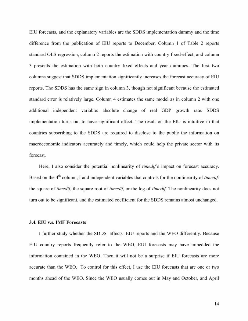
EIU forecasts, and the explanatory variables are the SDDS implementation dummy and the time

difference from the publication of EIU reports to December. Column 1 of Table 2 reports

standard OLS regression, column 2 reports the estimation with country fixed-effect, and column

3 presents the estimation with both country fixed effects and year dummies. The first two

columns suggest that SDDS implementation significantly increases the forecast accuracy of EIU

reports. The SDDS has the same sign in column 3, though not significant because the estimated

standard error is relatively large. Column 4 estimates the same model as in column 2 with one

additional independent variable: absolute change of real GDP growth rate. SDDS

implementation turns out to have significant effect. The result on the EIU is intuitive in that

countries subscribing to the SDDS are required to disclose to the public the information on

macroeconomic indicators accurately and timely, which could help the private sector with its

forecast.

Here, I also consider the potential nonlinearity of timedif’s impact on forecast accuracy.

Based on the 4th column, I add independent variables that controls for the nonlinearity of timedif:

the square of timedif, the square root of timedif, or the log of timedif. The nonlinearity does not

turn out to be significant, and the estimated coefficient for the SDDS remains almost unchanged.

3.4. EIU v.s. IMF Forecasts

I further study whether the SDDS affects EIU reports and the WEO differently. Because

EIU country reports frequently refer to the WEO, EIU forecasts may have imbedded the

information contained in the WEO. Then it will not be a surprise if EIU forecasts are more

accurate than the WEO. To control for this effect, I use the EIU forecasts that are one or two

months ahead of the WEO. Since the WEO usually comes out in May and October, and April

14

and September sometimes, the EIU forecasts employed will then be those in February, March,

April, July, August and September. When EIU reports and the WEO are published in the same

month, the EIU forecasts will be included in the estimation, as long as the EIU reports are

published ahead of the WEO.

Based on the above sample, I reexamine separately the effects of the SDDS on the WEO and

EIU reports. Table 3 shows that the SDDS has larger impact on the WEO than on EIU reports.

The impact of the SDDS on the EIU absolute forecast error is –0.56 (1st column), while its

impact on the WEO is higher at –0.71. During the sample period of 1996 to 2003, there were

some crisis periods, which decreased forecast accuracy significantly. I then exclude absolute

forecast errors that are bigger than four per cent. This shrinks the sample size by about nine per

cent. The new results are shown in the 3rd and 4th columns of Table 3. Again, the SDDS has

higher impact on the WEO than on EIU reports. The impact on the WEO is –0.37, while the

impact on EIU reports is only –0.16 and not significantly different from zero.

Table 4 presents the forecast accuracy of EIU reports and the WEO. Before SDDS

implementation, the average absolute forecast error across 16 countries and areas is 1.31 and

1.50 for EIU reports and the WEO respectively. So the WEO was especially inefficient, which is

consistent with Juhn and Loungani (2002).11 After SDDS implementation, the average decreases

to 1.10 and 1.07 for EIU reports and the WEO respectively. So before the SDDS, there is some

gap between EIU reports and the WEO, but SDDS implementation eliminates and if anything

reverses the gap.

11 They compare the WEO and Consensus Economics for the sample period 1989 to 1999, and find that the WEO is less accurate than Consensus Economics.

15

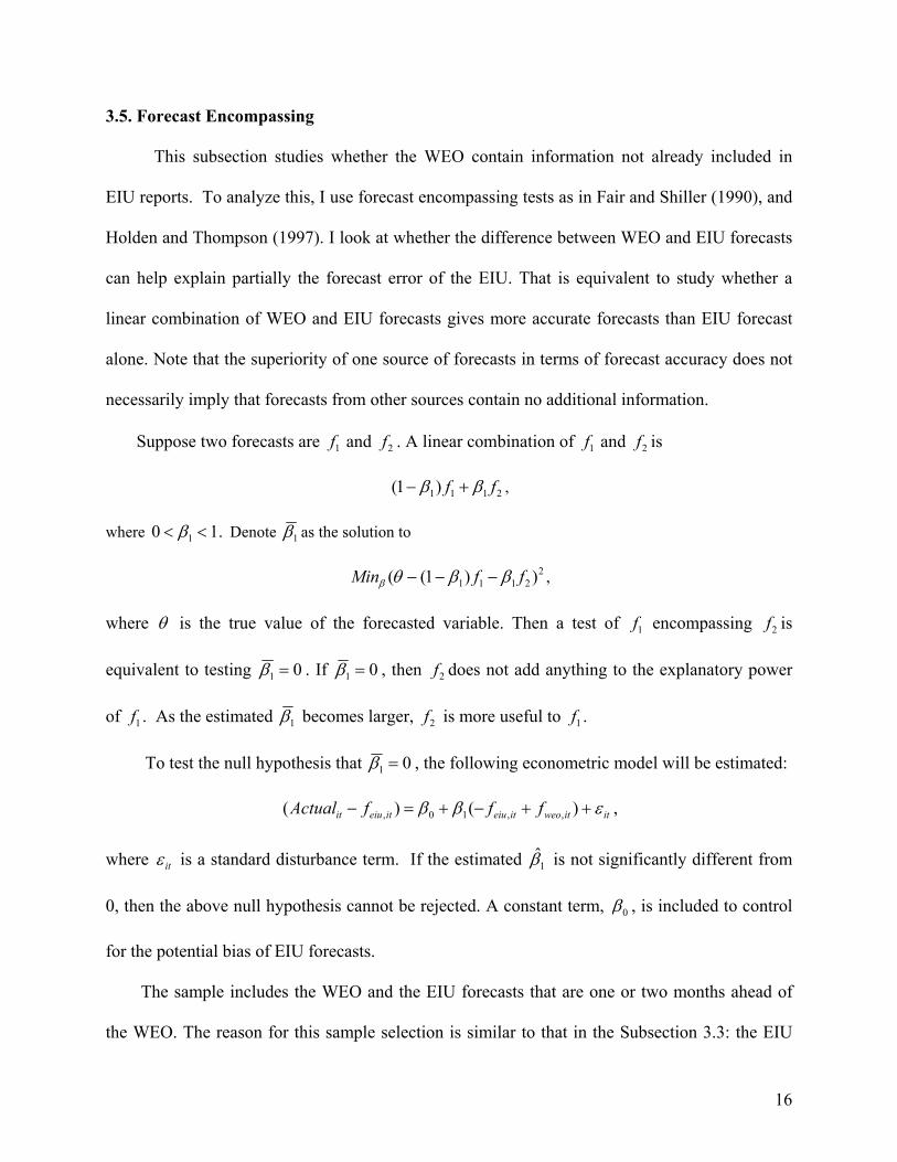
3.5. Forecast Encompassing

This subsection studies whether the WEO contain information not already included in

EIU reports. To analyze this, I use forecast encompassing tests as in Fair and Shiller (1990), and

Holden and Thompson (1997). I look at whether the difference between WEO and EIU forecasts

can help explain partially the forecast error of the EIU. That is equivalent to study whether a

linear combination of WEO and EIU forecasts gives more accurate forecasts than EIU forecast

alone. Note that the superiority of one source of forecasts in terms of forecast accuracy does not

necessarily imply that forecasts from other sources contain no additional information.

Suppose two forecasts are and . A linear combination of and is 1f 2f 1f 2f

2111)1( ff ββ +− ,

where .10 1 << β Denote 1β as the solution to

22111 ))1(( ffMin ββθβ −−− ,

where θ is the true value of the forecasted variable. Then a test of encompassing is

equivalent to testing

1f 2f

01 =β . If 01 =β , then does not add anything to the explanatory power

of . As the estimated

2f

1f 1β becomes larger, is more useful to . 2f 1f

To test the null hypothesis that 01 =β , the following econometric model will be estimated:

ititweoiteiuiteiuit fffActual εββ ++−+=− )()( ,,10, ,

where itε is a standard disturbance term. If the estimated is not significantly different from

0, then the above null hypothesis cannot be rejected. A constant term,

1̂β

0β , is included to control

for the potential bias of EIU forecasts.

The sample includes the WEO and the EIU forecasts that are one or two months ahead of

the WEO. The reason for this sample selection is similar to that in the Subsection 3.3: the EIU

16

forecasts published after the WEO may have imbedded the information from the WEO, and then

it is difficult to test whether the WEO is useful to EIU reports. Table 5 presents the

encompassing test. Before SDDS implementation, is 0.08, not significantly different from

zero (column 1). However, after SDDS implementation, becomes 0.45, significantly different

from zero at the 5% level (column 2). So after SDDS implementation, the WEO is no longer

encompassed by EIU reports.

1̂β

1̂β

Column 1 and 2 estimate the models separately for before and after SDDS implementation.

In column 3, I pool the before and the after together, and estimate the following model:

ititweoiteiuiteiuit ffSDDSSDDSfActual εββββ ++−+++=− ))(()( ,,3120, .

3β̂ , the impact of the SDDS on forecast encompassing, is large in value (0.36), but not

significantly different from zero. Probing deeper, forecast accuracy tend to be smaller during

financial crises. I then exclude extreme values owning to crises, and focus on the situations when

the absolute forecast error is less than four per cent.12 now becomes 0.45, significantly

different from zero at the 5 per cent level (column 4). So with the implementation of the SDDS,

the WEO is able to provide more information to EIU reports, but not during crisis periods.

3β̂

I find that both the IMF and the EIU missed financial crises and later-on economic

recovery. For example, both the WEO and EIU reports missed not only the 1998 financial crises

in Hong Kong, Korea, Malaysia and Thailand, but also the recovery in the second year. Even

after SDDS implementation, their ability of forecasting crises does not improve significantly. For

example, Argentina had a financial crisis in 2001. The May 2001 WEO forecast for Argentina

Real GDP growth rate was two per cent, and the April EIU forecast was 1.9 per cent. Both

significantly missed the coming crisis that caused the actual growth rate drop to be –4.4 per cent. 12 Recall that this shrinks the sample size by nine per cent.

17

So transparency does not necessarily provide better early warning of crises. Similarly, Argentina

had a recovery in 2003 with growth rate being 8.7 per cent. But in April 2003, both the EIU and

the IMF forecasted the growth rate being only three per cent. One possible explanation is that

their models for forecasting are linear, not suitable for forecasting extreme events such as crises.

Moreover, the current literature on crises, such as Obstfeld (1994), regards crises as a result of

multiple equilibria, which highlights the difficulty of forecasting crises.

I then look at the question the other way around, and examine whether the WEO

encompasses EIU forecasts. For this purpose, I use the EIU forecasts on the same month and

one-month after the WEO publication.13 The selected EIU reports thus will mainly be those

published in May, June, October and November. I focus on the situations when the absolute

forecast error is less than four per cent. The following econometric model is estimated:

ititeiuitweoitweoit fffActual εββ ++−+=− )()( ,,10, .

The estimated is significantly different from zero both before and after SDDS

implementation (column 1 and 2 of Table 6), so we reject the null hypothesis that the WEO

encompasses EIU forecasts. That is to say, EIU forecasts indeed can provide additional

information not contained in the WEO.

1̂β

This result is consistent with Juhn and Loungani (2002), who find that the WEO does not

encompass Consensus Economics. One explanation could be that EIU reports are published one-

month later than the WEO, thus EIU reports have additional information for that month that is

not inside the WEO. To check it, I further restrict the sample to where the WEO and EIU reports

are published in the same month. Again, I find that the WEO does not encompass EIU reports

13 Here I allow for same month sample because the WEO publication usually has one-month or two-month lags (Batchelor 2000).

18

(column 3 and 4 of Table 6).14 This suggests that private forecasts can provide valuable

information to international organizations.

4. Theoretical Model

In the above empirical estimations, there are two main findings:

• The SDDS increases the accuracy of the WEO more than that of EIU reports.

• Since SDDS implementation, combining the WEO and EIU reports will do significantly

better in forecasting than EIU reports alone.

I now develop an information model to reconcile these two findings. Note that the first

finding does not necessarily imply the second finding. It could well be the case that the

WEO has higher forecast accuracy but still contains no information that is not already inside

EIU reports. Moreover, both the EIU and the IMF have the same access to data disclosed by

the SDDS, which could make the second finding less likely to hold. However, I will show

that if the noisy term in public information from the SDDS is correlated with that in IMF’s

private information, then the WEO could potentially provide more information not already

in EIU reports. A contribution of the model here is that it provides a theoretical explanation

for the encompassing test, which has so far been largely presented as pure econometric

analyses. Furthermore, the model is the first one to explicitly analyze how the correlation

between public and private information affects the overall forecast accuracy.

14 Note that in column 4, is different from zero only at ten per cent significance level owing to relatively small

sample size. Still, is quite large at 0.69. 1̂β

1̂β

19

4.1. Basic Model

Suppose there are two agents, 2,1=i . Agent i receives both public information,

ηθ +=x , (1)

and private information,

ii uy +=θ . (2)

η is a normally distributed disturbance term, independent of the true fundamental value θ , with

mean zero and precision α (α =][

1ηVar

). is also normally distributed, independent of iu θ and

η , with mean zero and precision iγ ( iγ =]iVar[

1u

). Moreover, u and u are independent. 1 2 α and

iγ are known to agent i. I assume further that agent i only observe x and , but not . iy jy

Based on x and , agent i will form his or her forecast of iy θ according to the following

Bayesian updating rule as in Lyons (2001)15:

i

iii

yxfγαγα++

= . (3)

The variance of the forecast is if

i

if γα +=

1]var[ . (4)

Given the precision of private information ( iγ ), the marginal effect of public information

precision (α ) on is ]var[ if 2)(1

iγα +− .

The SDDS is assumed to affect only public information through simultaneous and free

disclosure of information to the public. The above formula for the marginal effect is consistent

15 See page 108 of Lyons (2001).

20

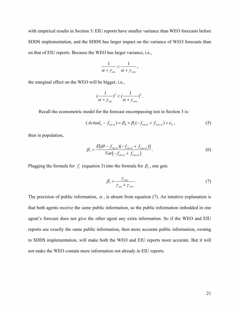
with empirical results in Section 3: EIU reports have smaller variance than WEO forecasts before

SDDS implementation, and the SDDS has larger impact on the variance of WEO forecasts than

on that of EIU reports. Because the WEO has larger variance, i.e.,

weoeiu γαγα +<

+11 ,

the marginal effect on the WEO will be bigger, i.e.,

22 )1()1(weoeiu γαγα +

<+

.

Recall the econometric model for the forecast encompassing test in Section 3 is:

ititweoiteiuiteiuit fffActual εββ ++−+=− )()( ,,10, , (5)

then in population,

][)])([(

,,

,,,1

itweoiteiu

itweoiteiuiteiu

ffVarfffE

+−+−−

=θ

β . (6)

Plugging the formula for (equation 3) into the formula for if 1β , one gets

weoeiu

weo

γγγβ+

=1 . (7)

The precision of public information, α , is absent from equation (7). An intuitive explanation is

that both agents receive the same public information, so the public information imbedded in one

agent’s forecast does not give the other agent any extra information. So if the WEO and EIU

reports use exactly the same public information, then more accurate public information, owning

to SDDS implementation, will make both the WEO and EIU reports more accurate. But it will

not make the WEO contain more information not already in EIU reports.

21

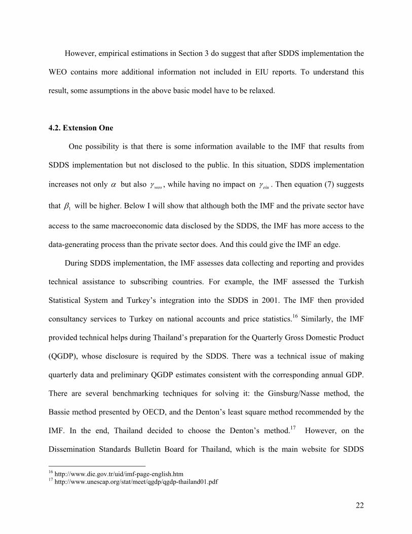
However, empirical estimations in Section 3 do suggest that after SDDS implementation the

WEO contains more additional information not included in EIU reports. To understand this

result, some assumptions in the above basic model have to be relaxed.

4.2. Extension One

One possibility is that there is some information available to the IMF that results from

SDDS implementation but not disclosed to the public. In this situation, SDDS implementation

increases not only α but also weoγ , while having no impact on eiuγ . Then equation (7) suggests

that 1β will be higher. Below I will show that although both the IMF and the private sector have

access to the same macroeconomic data disclosed by the SDDS, the IMF has more access to the

data-generating process than the private sector does. And this could give the IMF an edge.

During SDDS implementation, the IMF assesses data collecting and reporting and provides

technical assistance to subscribing countries. For example, the IMF assessed the Turkish

Statistical System and Turkey’s integration into the SDDS in 2001. The IMF then provided

consultancy services to Turkey on national accounts and price statistics.16 Similarly, the IMF

provided technical helps during Thailand’s preparation for the Quarterly Gross Domestic Product

(QGDP), whose disclosure is required by the SDDS. There was a technical issue of making

quarterly data and preliminary QGDP estimates consistent with the corresponding annual GDP.

There are several benchmarking techniques for solving it: the Ginsburg/Nasse method, the

Bassie method presented by OECD, and the Denton’s least square method recommended by the

IMF. In the end, Thailand decided to choose the Denton’s method.17 However, on the

Dissemination Standards Bulletin Board for Thailand, which is the main website for SDDS

16 http://www.die.gov.tr/uid/imf-page-english.htm 17 http://www.unescap.org/stat/meet/qgdp/qgdp-thailand01.pdf

22

disclosure, it only states “the revision of quarterly figures is calculated by using mathematical

technique so that the sum of four quarters must be equal to the annual estimate”, without

referring specifically to the Denton’s technique.18

So the IMF could have more influence and knowledge on the data-generating process than

the private sector, even though the data per se is disclosed to the public through the SDDS.19

Thus the IMF may be able to use the data more efficiently than private forecasters.

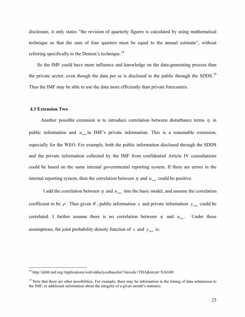
4.3 Extension Two

Another possible extension is to introduce correlation between disturbance terms η in

public information and in IMF’s private information. This is a reasonable extension,

especially for the WEO. For example, both the public information disclosed through the SDDS

and the private information collected by the IMF from confidential Article IV consultations

could be based on the same internal governmental reporting system. If there are errors in the

internal reporting system, then the correlation between

weou

η and could be positive. weou

I add the correlation between η and u into the basic model, and assume the correlation

coefficient to be

weo

ρ . Thus given θ , public information x and private information could be

correlated. I further assume there is no correlation between

weoy

η and . Under these

assumptions, the joint probability density function of

eiuu

x and is: weoy

18 http://dsbb.imf.org/Applications/web/sddsctycatbaselist/?strcode=THA&strcat=NAG00 19 Note that there are other possibilities. For example, there may be information in the timing of data submission to the IMF, or additional information about the integrity of a given month’s statistics.

23

,2)1(2

1exp

121),(

22

2

2

−+

−

−−

−−−

×−

=

weoweo

weo

u

weo

u

weo

u

weo

yyxx

yxf

σθ

σθ

σθρ

σθ

ρ

ρσπσ

ηη

η ( 8)

where ησ and weouσ are the standard errors of η and respectively. One can take the derivate

of the log of with respect to

weou

)weoy,(xf θ , and calculate the maximum likelihood estimator for

θ , , by setting the derivative equal to zero. The forecast of the WEO, , is always equal to

, which has the following form:

θ̂ weof

θ̂

.)(2

))(())((ˆ5.0

5.05.0

weoweo

weoweoweoweoweo

yxfαγργα

αγργαγραθ−+

−+−=≡ (9)

The forecast of the EIU, , is still the same as the one in the basic model: eiuf

eiu

eiueiueiu

yxfγαγα++

= . (10)

From equation (9), one can show that the variance of is: weof

5.0

2

)(21][

weoweoweofVar

αγργαρ

−+−

= . (11)

The sign of the derivative α∂

∂ ]var[ weof depends on the sign of . If the

correlation

)( 5.05.0 αργ −weo

ρ is negative, then is negative and )5.0α( 5.0ργ −weo 0]<

var[∂

∂α

weof , which means

higher precision of public information will increase IMF’s forecast accuracy.

However, when ρ is positive, it is more complicated. If (i.e., private

information is relatively imprecise), then

5.05.0 αργ <weo

0]var[<

∂∂

αweof , thus more public disclosure will

24

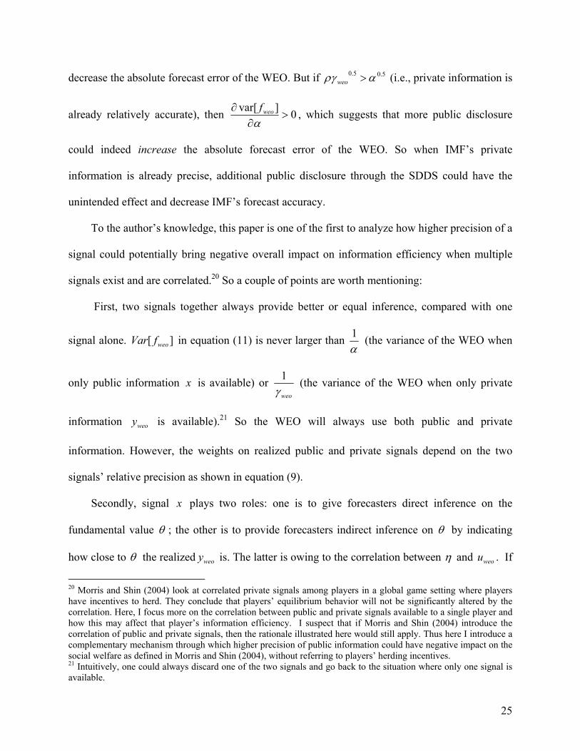
decrease the absolute forecast error of the WEO. But if (i.e., private information is

already relatively accurate), then

5.05.0 αργ >weo

0]var[>

∂∂

αweof , which suggests that more public disclosure

could indeed increase the absolute forecast error of the WEO. So when IMF’s private

information is already precise, additional public disclosure through the SDDS could have the

unintended effect and decrease IMF’s forecast accuracy.

α1

To the author’s knowledge, this paper is one of the first to analyze how higher precision of a

signal could potentially bring negative overall impact on information efficiency when multiple

signals exist and are correlated.20 So a couple of points are worth mentioning:

First, two signals together always provide better or equal inference, compared with one

signal alone. Var in equation (11) is never larger than ][ weof (the variance of the WEO when

only public information x is available) or weoγ1 (the variance of the WEO when only private

information is available).weoy 21 So the WEO will always use both public and private

information. However, the weights on realized public and private signals depend on the two

signals’ relative precision as shown in equation (9).

Secondly, signal x plays two roles: one is to give forecasters direct inference on the

fundamental value θ ; the other is to provide forecasters indirect inference on θ by indicating

how close to θ the realized is. The latter is owing to the correlation between weoy η and . If weou

20 Morris and Shin (2004) look at correlated private signals among players in a global game setting where players have incentives to herd. They conclude that players’ equilibrium behavior will not be significantly altered by the correlation. Here, I focus more on the correlation between public and private signals available to a single player and how this may affect that player’s information efficiency. I suspect that if Morris and Shin (2004) introduce the correlation of public and private signals, then the rationale illustrated here would still apply. Thus here I introduce a complementary mechanism through which higher precision of public information could have negative impact on the social welfare as defined in Morris and Shin (2004), without referring to players’ herding incentives. 21 Intuitively, one could always discard one of the two signals and go back to the situation where only one signal is available.

25

forecasters rely more on x ’s first role, then a positive weight will put on x in equation (9). In

the case where ][ηVar is extremely small, forecasters could just set the forecast equal to x .

However, if forecasters rely more on x ’s second role, then a negative weight might be put on x

in cases where ρ is positive.22 When , the weight on 5.05.0 α>weoργ x in equation (9) is negative,

which suggests that x ’s second role is the dominant one.

][η x

θ x θ

θ

5.05.0 α>weo x

x

]weo

1

ργ2

2−weo

As x becomes more precise (i.e., Var becomes smaller), could provide forecasters

more accurate direct inference on , because is fluctuating in a smaller band around .

However, at the same time, η becomes less capable of inferring , in that weou η has less variation

than before. That is to say, x is less capable of telling how close to the realized is. This

bears some analogy to traditional econometrical inference, where smaller variations in

explanatory variables tend to cause higher standard errors for estimated coefficients. The overall

effect of the higher precision of

weoy

x then depends on which one of the two effects dominates.

When , as shown earlier, ργ ’s second role is more important to forecasters. In

this case, because the higher precision of benefits x ’s first role and hurts its second role, the

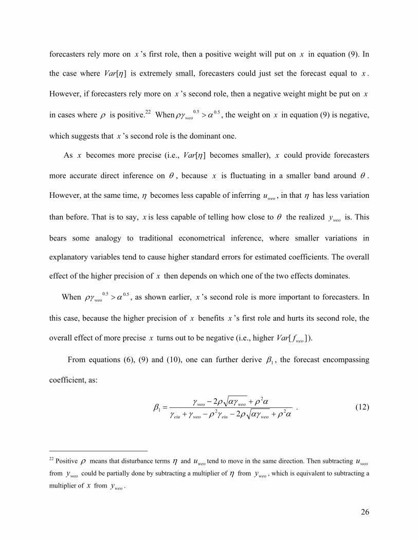
overall effect of more precise x turns out to be negative (i.e., higher Var ). [ f

From equations (6), (9) and (10), one can further derive β , the forecast encompassing

coefficient, as:

αραγργργγαραγ

β 2

2

1 2 +−−++

=weoeiuweoeiu

weo . (12)

22 Positive ρ means that disturbance terms η and tend to move in the same direction. Then subtracting u

from could be partially done by subtracting a multiplier of weou weo

weoy η from , which is equivalent to subtracting a

multiplier of weoy

x from . weoy

26

If the correlation coefficient ρ is zero, then we are back to equation (7) where the accuracy of

public information does not affect forecast encompassing at all. However, if ρ is different from

zero, then public information could affect forecast encompassing.

From equation (12), one can derive the derivative αβ∂∂ , whose sign depends on

. If (i.e., private information is relatively imprecise), then )( 5.05.0weoγρα − 5.05.0

weoγρα >αβ∂∂ >0,

and higher precision of public information from the SDDS will cause the WEO provide

additional information to the EIU.23 Thus, when , we have theoretical results that

are consistent with the empirical results in Section 3.

5.05.0weoγρα >

One can also think of other possible theoretical extensions that could support empirical

findings in Section 3. However, these extensions should be based on the real operating procedure

of the SDDS or the forecast-generating processes of the WEO and EIU reports as shown in the

above two extensions. As a future work, it will also be interesting to see which one of the two

extensions fits the real situation better. That is to say, whether it is the additional private

information or the correlation between public and private information that gives the IMF an

edge.

5. Conclusion

This paper studies how data transparency standards affect macroeconomic forecasts. I find

that the SDDS improves both the forecast accuracy of the WEO and EIU reports, with larger

23 Note that also implies , because the correlation coefficient 5.05.0

weoγρα > 5.05.0weoργα > ρ is between –1

and 1. When , as shown earlier, more accurate public information increases the forecast accuracy of the WEO.

5.05.0weoργα >

27

impact on the former. By applying encompassing tests, I further find that the WEO becomes

more informative to EIU reports after SDDS implementation. I then propose an information

model with correlated public and private signals to illustrate circumstances under which the

WEO could be more informative to EIU reports. If the process of SDDS implementation

provides the IMF with additional private information, or if the noisy term in public information

disclosed by the SDDS is correlated with that in IMF’s private information, then the SDDS could

cause the WEO to provide more information that has not been included in EIU reports.

28

Table 1. The Impact of the SDDS on the WEO

OLS (SDDS Countries)

OLS (SDDS Countries)

Random Country Effects (SDDS Countries)

Random Country Effects (All Countries)

Random Country-Year Pair Effects (All countries)

IMF Programs (All Countries)

1α (SDDS) -0.42 (0.10)

-0.47 (0.08)

-0.30 (0.17)

-0.28 (0.10)

-0.25 (0.12)

-0.24 (0.13)

2α (Timedif) 0.11 (0.02)

0.11 (0.02)

0.11 (0.02)

0.07 (0.01)

0.07 (0.01)

0.07 (0.01)

Absolute change in GDP growth rate

0.22 (0.02)

0.26 (0.02)

0.17 (0.01)

0.16 (0.02)

0.16 (0.02)

IMF program 0.33 (0.17)

IMF program interacted with SDDS

-0.13 (0.23)

Year 1997 0.32 (0.23)

0.33 (0.13)

0.38 (0.17)

0.34 (0.17)

Year 1998 0.13 (0.23)

0.10 (0.13)

0.15 (0.17)

0.15 (0.17)

Year 1999 0.31 (0.22)

0.28 (0.13)

0.31 (0.17)

0.29 (0.17)

Year 2000 0.13 (0.19)

0.28 (0.12)

0.31 (0.16)

0.28 (0.16)

Year 2001 0.16 (0.17)

0.13 (0.11)

0.13 (0.15)

0.17 (0.15)

Year 2002 0.01 (0.16)

0.12 (0.11)

0.06 (0.14)

0.05 (0.14)

Year 2003

Constant 0.87 (0.11)

0.48 (0.1)

0.16 (0.24)

0.61 (0.13)

-0.43 (1.01)

1.57 (1.00)

No. of observation

785 685 685 1273 1273 1249

R-squared 0.06 0.40 0.41

0.25 0.52 0.52

Note: Standard errors are in parentheses. Coefficients different from zero at 5% level are in bold.

29

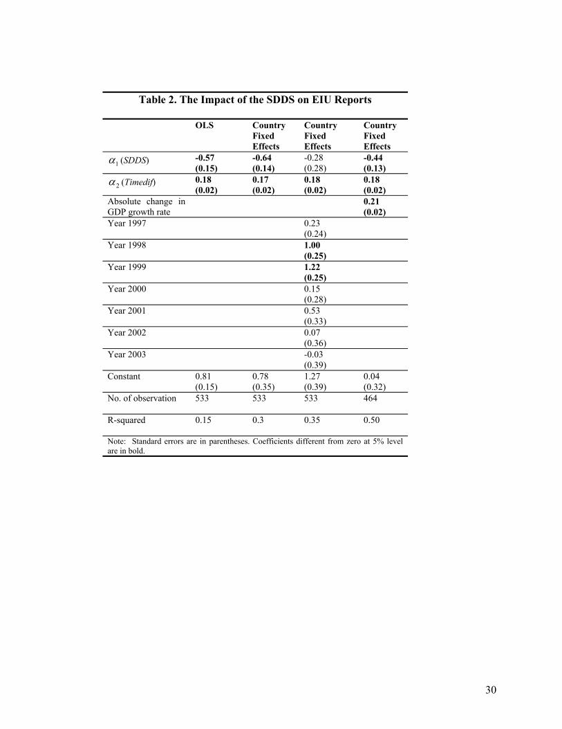
Table 2. The Impact of the SDDS on EIU Reports OLS Country

Fixed Effects

Country Fixed Effects

Country Fixed Effects

1α (SDDS) -0.57 (0.15)

-0.64 (0.14)

-0.28 (0.28)

-0.44 (0.13)

2α (Timedif) 0.18 (0.02)

0.17 (0.02)

0.18 (0.02)

0.18 (0.02)

Absolute change in GDP growth rate

0.21 (0.02)

Year 1997 0.23 (0.24)

Year 1998 1.00 (0.25)

Year 1999 1.22 (0.25)

Year 2000 0.15 (0.28)

Year 2001 0.53 (0.33)

Year 2002 0.07 (0.36)

Year 2003 -0.03 (0.39)

Constant 0.81 (0.15)

0.78 (0.35)

1.27 (0.39)

0.04 (0.32)

No. of observation 533

533 533 464

R-squared 0.15 0.3 0.35

0.50

Note: Standard errors are in parentheses. Coefficients different from zero at 5% level are in bold.

30

Table 3. Comparing SDDS’s Impact on EIU and IMF Forecasts

EIU Forecast

IMF Forecast

EIU Forecast

IMF Forecast

1α (SDDS) -0.56 (0.21)

-0.71 (0.23)

-0.16 (0.14)

-0.37 (0.17)

2α (timedif) 0.17 (0.04)

0.17 (0.05)

0.08 (0.03)

0.09 (0.03)

No. of observation 193

193 176 176

R-squared 0.31 0.30

0.28 0.25

Note: Standard errors are in parentheses. Coefficients different from zero at 5% level are in bold. Estimations cover 16 countries with country fixed-effect included. Columns 1 and 2 include extreme values. Columns 3 and 4 exclude extreme values.

31

Table 4. EIU vs. WEO Forecasts

EIU absolute forecast error (Mean)

WEO absolute forecast error (Mean)

Before the SDDS 1.31

1.50

After the SDDS 1.10 1.07

Note: Extreme forecast errors (lager than 4% in absolute sense) are excluded.

32

Table 5. Testing Whether EIU Reports Encompass the WEO

Before SDDS After SDDS Pooled Estimation No extreme value

0β -.37 (0.24)

0.15 (0.19)

-0.37 (0.21)

-.27 (0.15)

1β 0.08 (0.22)

0.45 (0.22)

0.08 (0.20)

0.02 (0.15)

2β 0.51 (0.31)

0.37 (0.22)

3β 0.36 (0.33)

0.45 (0.23)

No. of observations

110 95 205 189

R-squared 0.001 0.04 0.03 0.05

Note: standard errors are in the parentheses. Coefficients different from zero at 5% level are in bold.

33

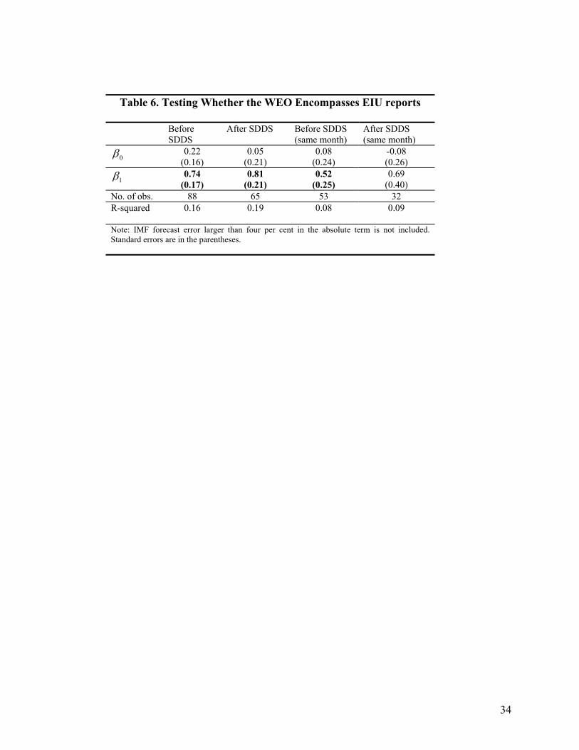
Table 6. Testing Whether the WEO Encompasses EIU reports

Before SDDS

After SDDS Before SDDS (same month)

After SDDS (same month)

0β 0.22 (0.16)

0.05 (0.21)

0.08 (0.24)

-0.08 (0.26)

1β 0.74 (0.17)

0.81 (0.21)

0.52 (0.25)

0.69 (0.40)

No. of obs. 88 65 53 32 R-squared 0.16 0.19

0.08 0.09

Note: IMF forecast error larger than four per cent in the absolute term is not included. Standard errors are in the parentheses.

34

35

References:

1. Artis, Michael J (1996), “How Accurate are the IMF's Short-Term Forecasts? Another Examination of the World Economic Outlook,” International Monetary Fund Working Paper: WP/96/89.

2. Balke, Nathan S and D'Ann Petersen (2002), “How Well Does the Beige Book Reflect Economic Activity? Evaluating Qualitative Information Quantitatively,” Journal of Money, Credit, and Banking 34, pp. 114--136

3. Barrionuevo, Jose M (1992), “A Simple Forecasting Accuracy Criterion under Rational Expectations: Evidence from the World Economic Growth Outlook and Time Series Models,” International Monetary Fund Working Paper: WP/92/48.

4. Batchelor, Roy (2000), “The IMF and OECD versus Consensus Forecasts,” London City University Business School Working Paper.

5. Batchelor, Roy and Pami Dua (1991), “Blue Chip Rationality Tests,” Journal of Money, Credit and Banking 23 (4), pp. 692-705.

6. Beach, William, Aaron B. Schavey, and Isabel M. Isidro (1999), “How Reliable Are IMF Economic Forecasts?” Heritage Foundation Center for Data Analysis Report #99-05.

7. Clark, Alastair and John Drage (2000), “International Standards and Codes,” Financial Stability Review, pp. 162--168.

8. Davies, Anthony and Kajal Lahiri (1995), “A New Framework for Analyzing Survey Forecasts Using Three-Dimensional Panel Data,” Journal of Econometrics 68(1), pp. 205--227.

9. De Masi, Paula (1996), “The Difficult Art of Economic Forecasting,” Finance and Development 33, pp. 29--31.

10. Faust, J., J.H Rogers, and J.H. Wright (2003), “News and Noise in G-7 GDP Announcements,” Working Paper No. 690, Board of Governors of the Federal Reserve System.

11. Fair, Ray, and Robert Shiller (1990), “Comparing Information in Forecast from Econometric Models,” American Economic Review 80 (3), pp. 375--389.

12. Gavin, William T and Rachel J Mandal (2001), “Forecasting Inflation and Growth: Do Private Forecasts Match Those of Policymakers?” Federal Reserve Bank of St. Louis Review 83(3), pp. 11-19.

13. Graham, John R. (1996), “Is a Group of Economists Better Than One? Than None?” Journal of Business 69 (2), pp. 193--232.

14. Juhn, Grace and Prakash Loungani (2002), “Further Cross-Country Evidence on the Accuracy of the Private Sector's Output Forecasts,” IMF Staff Papers 49(1), pp. 49--64.

15. Lyons, Richard (2001), The Microstructure Approach to Exchange Rates, the MIT Press. 16. Obstfeld, Maurice (1994), “The Logic of Currency Crises,” NBER Working Paper 4640. 17. Peterson, Steven P (2001), “Rational Bias in Yield Curve Forecasts,” Review of

Economics and Statistics 83(3), pp. 457--64. 18. Swidler, Steve, and David Ketcher (1990), “Economic Forecasts, Rationality, and the

Processing of New Information over Time,” Journal of Money, Credit and Banking 22 (1), pp. 65--76.