Do This to Decide to Continue or Drop Out

7/23/2019 Do This to Decide to Continue or Drop Out

http://slidepdf.com/reader/full/do-this-to-decide-to-continue-or-drop-out 1/31

1 - 31

ECON 2310

Intermediate Microeconomics

Algebra Review

This course does not require any calculus or “high level” mathematical techniques.

However, a comprehensive understanding of basic, elementary algebra and

complementary graphs is required. Although most of the mathematics used in this coursewill have been covered in highschool (grades 9, 10 and 11), it is important that you take

this review and preparation of algebra seriously. Many students never fully understand

the models used in economics simply because they lack a full understanding of the

simple mathematics underlying them. If you haven’t recently taken a course with a

substantial amount of algebra in it, you may have forgotten some of the basics.

So check out this algebra review. Do the Pre-Test to determine your current

level of understanding of relevant algebra and graphs. If it isn’t completely solid spend

some time on the learning modules. Then re-do the Pre-Test. If you are still having

some difficulty with the material you should get a textbook on elementary algebra or

perhaps an appropriate Schaum’s Outlines on Elementary Algebra and spend some timebecoming comfortable with the required mathematics. A review of relevant arithmetic

and algebra is also provided in the book Mathematics for Economics Student’s

Solutions Manual , by M. Hoy, J. Livernois, C. McKenna, R. Rees, and T. Stengos,

Addison Wesley Publishers, 1996, Chapter 1 Algebra and Arithmetic Reviews and

Self-tests (pages 1 to 26).



ECON*2310 Intermediate M1croeconomics Fall 2001

2 - 31

( x y)( x

y) (2 x

1)

( x

y )( y

2 xy

x

x)

3 x ( x y )

1

x

x

y

x

x

y

x y

x

y

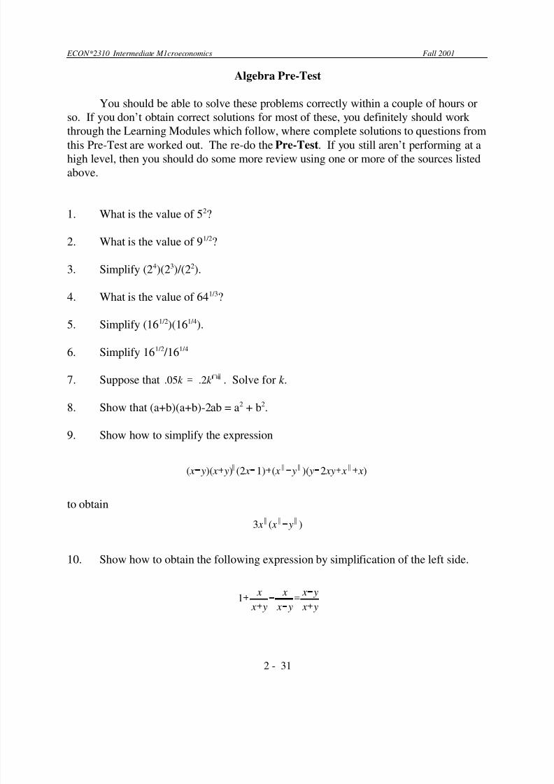
Algebra Pre-Test

You should be able to solve these problems correctly within a couple of hours or

so. If you don’t obtain correct solutions for most of these, you definitely should work

through the Learning Modules which follow, where complete solutions to questions from

this Pre-Test are worked out. The re-do the Pre-Test. If you still aren’t performing at a

high level, then you should do some more review using one or more of the sources listed

above.

1. What is the value of 52?

2. What is the value of 91/2?

3. Simplify (2

4

)(2

3

)/(2

2

).

4. What is the value of 641/3?

5. Simplify (161/2)(161/4).

6. Simplify 161/2 /161/4

7. Suppose that . Solve for k ..05k .2k

8. Show that (a+b)(a+b)-2ab = a

2

+ b

2

.

9. Show how to simplify the expression

to obtain

10. Show how to obtain the following expression by simplification of the left side.




3 - 31

11. Draw the graph of the function q=25-2p, placing q on the horizontal axis and p on

the vertical axis.

12. Draw the graph of the function q=-5+p, placing q on the horizontal axis and p onthe vertical axis.

13. Let Q=aL, a>0 a parameter, be a function representing the total product of labour.

Sketch this graph and illustrate the fact that a given increase in L (labour) always

leads to the same increase in Q (output) regardless of the initial level of L.

14. Sketch the graph for the function Q=10L1/2. Indicate the values of Q at L=1, L=4,

L=9 and illustrate the fact that increasing L has a lesser impact on increasing Q the

greater is the level of L.

15. Sketch the graph for the function Q=L2. Indicate the values of Q at L=1, L=4,

L=9 and illustrate the fact that increasing L has a greater impact on increasing Q

the greater is the level of L.

16. Draw the function for the equality 4x1 + x2 = 120, with x2 on the vertical axis and

x1 on the horizontal axis. Restrict x1 and x2 to be non-negative (i.e., x1

0 and x2

0). Shade in those points which satisfy the inequality 4x 1 + x2

120.

17. Find the partial equilibrium solution (demand = supply) for the following:

demand: q = 25 - 2p

supply: q = -5 + p

and illustrate with a graph.




4 - 31

Brief Solutions

1. 25

2. 3

3. 25 = 32

4. 4

5. 163/4 = 8

6. 161/4 = 2

7. k = 16. See Module 1: sections on Power Rules

8. See Module 1:Basic Arithmetic Operations, Including Powers, section on

Manipulating Expressions (Expand, Factor, Simplify, Solve).

9. See Module 1:Basic Arithmetic Operations, Including Powers, section on

Manipulating Expressions (Expand, Factor, Simplify, Solve).

10.. See Module 1:Basic Arithmetic Operations, Including Powers, section on

Division and Common Denominators.

11.




5 - 31

12.

NOTE: for more discussion of solutions to questions 10 and 11 see Module 2: Linear

Functions and Their Graphs

13.




6 - 31

14.

L 0 1 4 9

Q=10

L or

Q=10L1/2

0 1

0

20 30

Q - 1

0

2.6

8

1.7

2

We sketch this

function, Q=10

L below

15.




7 - 31

L 0 1 4 9

Q=L2 0 1 16 81

Q - 1 7 17

We sketch this function, Q=L2 on the next page.




8 - 31

NOTE: For more

details on the

solutions for questions 12, 13 and 14, see

Module 3: Simple

Nonlinear Functio

ns and Their

Graphs.

16. Rewrite the

equation as x2 = 120

- 4x1 makes this easy

to graph. Theregion that should

be shaded in represen

ts the set of points

which satisfy

the inequalit

y

4x1 + x2 120.

17.




9 - 31

NOTE: For more discussion of the solution to question 15 see Module 4: Functions and

Inequalities. For more discussion of the solution to question 16 see Module 5: Solving

Systems of Linear Equations.

Learning Modules




10 - 31

Note that these learning modules are not comprehensive reviews of the

mathematical topics addressed but rather are intended to be short reviews to help those

who have forgotten some of the basics that are essential to this course. When possible,

we use applications from economics that you have already learned in introductory

economics or ideas for which no economic’s background is required. If this reviewmaterial proves not to be sufficient for you, then you will need to take a more aggressive

approach to reviewing the mathematical background required for this course.

Module 1: Basic Arithmetic Operations, Including Powers

In this, and following modules, letters such as a, b, c, d, x, y, z are used to

represent real number values. Rules for manipulating expressions are generally given in

terms of “unspecified” numbers but we will usually provide specific examples with

specific numbers as well. These rules are used to manipulate and simplify or solve for

expressions.

Commutative Law of Addition: a+b = b+a

This law simply indicates that adding two numbers together gives the same answer

regardless of the order in which they are added. So, for example, 5+2=7 and also 2+5=7.

This law can be applied iteratively and so the addition of any number of terms is also

independent of the order of addition. Thus, a+b+c = a+c+b = c+a+b = c+b+a, etc. So,

for example, 8+6+(-4) = 10 as is 6+(-4)+8 = 10.

Commutative Law of Multiplication: ab = ba

This law simply indicates that multiplying two numbers together gives the same answer

regardless of the order in which they are multiplied. So, for example, 3×6=18 and also

6×3=18. As with the case for addition, this law can be applied iteratively and so the

multiplication of any number of terms is also independent of the order of multiplication.

Thus, a×b×c = a×c×b = c×a×b = c×b×a, etc. So, for example, 3×7×2 = 42 as is 2×3×7 =

42.

Associative Law: (a+b)(c+d)=ac+ad+bc+bd

This law can be illustrated in two steps:

Step 1 (a+b)(c+d) = a(c+d) + b(c+d)

Step 2 a(c+d) + b(c+d) = ac+ad+bc+bd




11 - 31

If there are more than two terms to be added in one of the brackets then the associative

law continues to apply, just iteratively. Thus, (a+b)(c+d+e) = (a+b)((c+d)+e) =

(a+b)(c+d)+(a+b)e = ac+ad+bc+bd+ae+be = ac+ad+ae+bc+bd+be. In words, to expand

this expression multiply the first element in the left hand bracket (a) by each of the

elements in the right hand bracket (c,d,e), adding all the results together (ac+ad+ae), andthen do the same with the second element in the left hand bracket (b) to get (bc+bd+be),

and then add all terms together.

You can check the associative law with a specific numerical example, such as

(5+2)(6+8) = (5×6)+(5×8)+(2×6)+(2×8) = 30+40+12+16 = 98, noting that (5+2)(6+8) =

(7)(14) = 98.

Powers and Roots

There are several useful rules for simplifying expressions involving powers

(exponents) and roots. Although you would profit from a more thorough review of

powers (see Mathematics for Economics Student’s Solutions Manual , by Hoy, et al.,pages 4 to 6) the following condensed review contains most of the operations you will

require.

The square of a number is obtained by multiplying the number by itself (e.g., the

square of 5 is just 5×5 = 25). The square root is the inverse operation - that is, finding

the square root of a number, z (often written z), is finding that number which, when

multiplied by itself, gives the result z (e.g., the square root of 9 is 3, written 9 = 3).

Since finding the square root of a number, z, is the inverse operation of finding the

square of a number, we also write

z as z1/2. The rationale for this notation is that ½ is

the inverse of the number 2. If we multiply a number by itself 3 times we indicate this as

z×z×z = z

3

and refer to the result as the cube of z. So, for example, the cube of 4 is 64and we can write 43 = 4×4×4 = 64. The number, which when multiplied by itself three

times gives the value of some original number, say y, is called the cube root of y. So, for

example, the cube root of 64 is 4. Since finding the cube root is the inverse operation of

finding the cube of a number we write the cube root of a number y as y1/3. Thus, we say

641/3 = 4.

The above operations of multiplying a number by itself two or three times can be

extended to any number of times, n, and so we use the notation zn to represent the result

of multiplying the number z by itself n times and y1/n represents the result of finding the

number which, when multiplied by itself n times will give the number y. That is:

z×z×z×...z×z = zn

and y1/n

×y1/n

×y1/n

×...×y1/n

×y1/n

= y , where in each case there are “nmultiplications.

The following rules of powers follow directly from these definitions:

Power Rule for Inversions: If ya = x, then x = y1/a (e.g., if y2 = x, then x =

y1/2)




12 - 31

sak 1/2 k

This result is not generally noted explicitly as a rule for powers since it is really just a

restatement of the inverse operation of taking powers (e.g., the relationship between

finding the square of a number or the inverse operation of finding the square root of a

number). However, it is so useful it is included here explicitly.

Power Rule for Multiplication: (ya)(yb) = ya+b

For example, (25 )(22) = 25+2 = 27 since (2×2×2×2×2)×(2×2) gives the result of 2 being

multiplied by itself 7 times.

Power Rule for Division: ya /yb = ya-b

For example, 25 /22 = 25-2 = 23 since (2×2×2×2×2)/(2×2) = 2×2×2.

The power rule for division applies even if a-b is a negative number with theconvention that y-n represents 1/yn. These rules also apply for non-integer values of the

exponents. Another useful convention is y0 = 1 for any number y. This makes sense

once you note that using the power rule for division implies ya /ya = ya-a = y0 = 1 for any

numbers y and a, y not zero.

An example using the power rules.

In Macroeconomics we study the topic of economic growth. A typical problem that the

student encounters is to determine the steady state per capita capital stock of an economy

given an exogenous savings rate, capital depreciation rate, and a production function.

The fundamental relationship used to find the steady state capital stock is given by

equating savings to depreciation or , where s is the savings rate, f(k) is the per capitals f (k )

k

production function, k the per capita capital stock, and is the capital depreciation rate. If

savings (addition to the capital stock as savings equals investment) equals depreciation (the

reduction in the capital stock) the net gain in capital is zero and we say the economy is in

a steady state (capital is unchanging).

Suppose the per capita production function is given by . When savings equalsak 1/2

depreciation the steady state capital stock can be found by solving for k in the equation

Using the power rule for division this equation can be rewritten as






14 - 31

( x y)( x y)2(2 x 1) ( x 2 y 2)( y 2 xy x 2

x)

( x

y)( x

y)2(2 x

1)

( x

y)( x

y)( y

2 xy

x 2

x)

( x y)( x y)[( x y)(2 x 1) ( y 2 xy x 2 x)]

( x y)( x y)[2 x 2 x 2 xy y y 2 xy x 2

x]

( x y)( x y)[3 x 2]

3 x 2( x 2

y 2)

expand it. For example, to simplify (a+b)(a+b)-2ab expand (a+b)(a+b) to get (a+b)(a+b)

= a2 + ab + ba + b2 = a2 + 2ab +b2, since ba=ab by the commutative law. Thus, we obtain

(a+b)(a+b)-2ab = a2 + 2ab +b2 - 2ab = a2 + b2. To simplify expressions it is sometime

better not to expand every sub-expression and then collect terms but rather to “artfully”

combine factoring and expanding. For example, to simplify the expression

note that x2-y2 = (x-y)(x+y) and so we can rewrite the above equation as

and so noting that (x-y)(x+y) represents a common factor in both sub-expressions we can

rewrite the equation as

Expanding and collecting terms in for that part of the expression in square brackets, [ ],

gives

which results in the expression

or

Knowing how to expand, factor and simplify expressions is indispensable in

solving equations for unknown values.

Division and Common Denominators

In some instances dividing fractions by finding the common denominator is a

trivial matter. For example, to find the result for we note that the two terms have1

2

1

4




15 - 31

1

2

2

7

5

8

(1×7×8)

(2×2×8)

(5×2×7)

(2×7×8)

56

32

70

112

158

112

79

56

ab

e f

(a× f )

(e×b)(b× f )

af

ebbf

1

x

x

y

x

x y

x y

x

y

1

x

x

y

x

x y

1( x

y)( x y)

x( x y) x( x

y)

( x

y)( x y)

( x 2 xy

xy y 2)

x 2 xy x 2 xy

( x

y)( x y)

common denominator 4, with and so we have = = = . Once one1

2

2

4

1

2

1

4

2

4

1

4

(2

1)

4

3

4

takes into consideration more complicated expressions appearing in the denominator one

needs to be a bit more methodical about this. For example, consider the following

simplification:

Notice that to compute expressions such as the above first find the common

denominator by multiplying together the denominators of each fraction in the series

(2×7×8) and then for each fraction we multiply the numerator by the values of the

denominators of the other fractions. The rule is easiest to see when using fractions which

are ratios of variable names, such as the following:

So, you can use this simple rule to obtain simplifications of expressions such as

To see how to obtain this result note that the common denominator for this expression is(x+y)(x-y) and so this expression can be expanded and then simplified as shown below.




16 - 31

Then just collect terms on the numerator and divide out the (x-y) part.




17 - 31

y

mx

b

x

y

m

b

m

Module 2: Linear Functions and Their Graphs

In economics we often use linear functions in examples and illustrations because

of their simplicity. Although actual relationships between economic variables often are

not linear, the use of linear functions as approximations is often useful and reasonable.It is important to realize that when using a general functional notation, such as

y=f(x) - where we say y is a function of x - or a specific linear notation, such as y= mx+b,

to describe a relationship between two variables, one must not presume any direction or

notion of causality such as “a change in x causes a change in y” although, in some

circumstances, this may be an appropriate interpretation. For example, if the relationship

is between x, the level of labour used as an input into production, and y, the level of

output produced, then the notion of causality does make sense with changes in the level

of x causing or resulting in changes in the level of y. In particular, if y=5x describes

some linear production function, with x representing the number of person-hours used

and y the number of units of some product produced, the it does make sense to think of “changes in x” causing “changes in y” according to the function y=5x. However, even

when there is a clear notion of causality we can still write the function equivalently as

x=0.2y [or x=(1/5)y] and note that in this form we are expressing the idea that for every y

units of output the firm wishes to produce it needs to employ x=0.2y units of input. This

would allow us to determine the labour costs for producing any given level of output y as

CL = wx = 0.2wy, where w is the cost per person hour of labour, and so we can write

CL(y) = 0.2wy as the “cost of labour” function.

As noted above, one general way to denote a linear function, for y=f(x), is to write

where m and b are constants.

Note that in the inverse form this same relationship can be written

It is often useful to write linear equations in both “direct” form and “inverse” form in

order to easily find the intercept terms which are helpful in plotting the graph of thefunction. For the case above, the y intercept (i.e., the value of y when x is zero) is b

while the x intercept (i.e., the value of x when y is zero) is -b/m. The term m represents

the slope of the linear function and the fact that this slope is the same regardless of the

choice of the value of x is the key property of a linear function. If m is a positive value

(m>0) that means the function has a positive slope while if m is a negative number (m<0)

that means the function has a negative slope. If m=0 then the value of y is the same




18 - 31

(y=b) for all values of x. Each of these cases is illustrated in the following graphs.

Note that in each case above we placed y on the vertical axis and x on the

horizontal axis. Although this is often the choice made any such choice is,

mathematically speaking, arbitrary.

In economics we consider the demand function as quantity demanded being a

function of price, and write q = f(p) (or qd = f(p), with the subscript d included sometimes

just to indicate that the quantity refers to demand and not supply). Thus, one might




19 - 31

expect that we would use the horizontal axis to measure price, p, and the vertical axis to

measure quantity, q. However, the convention is just the opposite. Thus, if given the

function q = 25-2p it is a good idea to also write it in its inverse form, p = 12.5-0.5q in

order to facilitate graphing the function with q on the horizontal axis and p on the

vertical axis. It is also useful to write out demand and supply functions (and many othersas well) in direct (or original) form and also the inverse form as this makes it very simple

to compute the intercepts and hence more easily draw the graph.

We draw the graph for the above mentioned example below. Note that, since

q = 25-2p or, in inverse form, p = 12.5-0.5q, the q-intercept is 25 while the p-intercept is

12.5. Since the function is linear the graph of the function can be drawn by simply

drawing a straight line which

connects the intercept points

(q,p)=(0,12.5) for the p-intercept

and (q,p) = (25,0) for the q-

intercept. The graph is illustratedbelow.

Since negative values for a price or a quantity are not meaningful, we often do notextend the demand function into the regions where q<0 or p<0. The p-intercept for

demand functions (12.5 in this example) is sometimes referred to as the choke price since

it is the (smallest) price at which quantity demanded becomes zero (i.e., demand is

choked off). The q-intercept value for demand functions (q=25 in this example) is the

quantity that would be demanded if price were zero.

Consider next an example of a linear supply function, also quantity being a




20 - 31

function of price. Suppose q=-5+p, so that the slope of the supply function is 1 and the

intercepts are q=-5 for the q intercept and p=5 for the p intercept. The p intercept is the

value of p when q=0 and so for this example we have that unless p exceeds the value of

5, output will be zero. Of course, according to the function when p is less than zero the

value of q is negative, but negative values can’t be produced by the firm and so that justmeans no output is

produce for p<5. The q

intercept of -5 is not really

meaningful in an economic

sense since negative

quantities can’t be produced.

So for any values of p

which induce values of q

which are negative, the

actual amount produced ispresumed to be zero. In fact,

the relevant parts of the

graphs for both demand and

supply functions are

those parts that lie in the

positive quadrant (i.e.,

where both p 0 and q 0).

The supply function q=-5+p, which can also be written in its inverse form, p=q+5,

is illustrated in the graph below.




21 - 31




22 - 31

Module 3: Simple Nonlinear Functions and Their Graphs

Although we often use linear functions for examples and illustrations in

economics, in this course we will also need to use some simple nonlinear functions. The

fact that linear functions have constant slopes is precisely why we cannot always usethem to illustrate important economic properties.

Consider, for example, a simple linear production function, Q=aL, with a>0 a

pararmeter, which describes the relationship between the amount of input labour (L) used

and the level of output produced (Q). Since we are considering variations in the level of

only one input, labour, this function is sometimes called the total product of labour

function and its graph the total product of labour curve. The implication, generally, is

that other inputs - and in particular capital or machinery - is held at some fixed level.

This makes sense in a short-run setting since one can employ existing workers more

intensively, through overtime, or hire new workers in a much shorter time period than

can one set up new production lines and factories. Linearity of the function means thatan increase in one unit of L leads to an increase in output in the amount of “a” units

regardless of the existing level of labour employed. This is illustrated in the following

graph.

Since the amount of capital (machinery) is fixed it makes sense that the amount of




23 - 31

extra output generated by adding more labour will depend on the existing amount of

labour employed. The more labour already using the fixed amount of machinery, the less

might be the added amount of output per additional unit of labour employed. If this is

the case, we would say that labour is subject to the law of diminishing marginal

productivity. Since the slope of a function indicates the rate at which the variable on thevertical axis rises (or falls for a negative sloped function) and a “flatter” function means

this rate is lower, then according to our above description of what might happen when

more labour is used we should expect the slope of the total product of labour curve to fall

as more labour is added. A function with this property is Q=10 L or Q=10L1/2. The

following table gives some values which can be used to plot this function. From the

table, it is also clear that adding an extra unit of labour indicates less and less of an

increase in output.

L 0 1 2 3 4 5 6 7 8 9 10

Q=

L 0 10 14.1 17.3 20 22.36 24.5 26.5 28.3 30 31.62

Q - 10 4.14 3.18 2.7 2.36 2.14 1.96 1.84 1.72 1.62

We sketch this function, Q=10 L, below.




24 - 31

We generally expect that with a fixed amount of machinery (capital), additional

amounts of labour will at least eventually lead to smaller amounts of additional output.

That is, the law of diminishing marginal productivity of labour will eventually apply.

However, it is certainly possible that at zero or low levels of existing labour beingemployed, additional amounts of labour will not add so much to output. It is quite

plausible that the number of machines along a production process could not be used very

productively until a certain threshold level of labour were employed since with small

numbers of workers there would be a lot of running around from machine to machine in

order to generate any output. So additional output from additional units of labour may

well be created at an increasing rate, rather than a diminishing rate, at least for low levels

of output.

Again, since the slope of a function indicates the rate at which the variable on the

vertical axis rises and a “steeper” function means this rate is higher, then according to our

above description of what might happen when more labour is used we should expect theslope of the total product of labour curve to rise (at least initially) as more labour is

added. A function with this property is Q=L2. The following table gives some values

which can be used to plot this function. From the table, it is also clear that adding an

extra unit of labour indicates less and less of an increase in output.

L 0 1 2 3 4 5 6 7 8 9 10

Q=L2 0 1 4 9 16 25 36 49 64 81 100

Q - 1 3 5 7 9 11 13 15 17 19

We sketch this function,

Q=L2 below.




25 - 31

A function which is increasing with the slope becoming flatter as one moves from

right to left, such as the function Q=10

L , isconcave

. A function which is increasingwith the slope becoming steeper, such as the function Q=L2, is convex. A function with a

constant slope, of course, is linear. It is, of course, possible that a function will have

some segments which are convex and concave, and also may include segments which are

linear. In particular, suppose we think about the total product of labour function, and its

graph, in light of our above discussion. A plausible scenario is that the shape of the total

product curve is convex for low levels of labour but that it becomes concave at levels of

labour sufficie

ntly high that the

law of diminis

hing marginal product

ivity applies.

Such a functio

n would have

the shape illustrat

ed in the graph

below.




26 - 31

The simplest function which has the above shape for its graph is a cubic function.

We won’t investigate further here how to determine the graph of a cubic function as suchspecific exercises are not so important in this course. However, you do need to

understand the meaning of convex and concave shapes of functions in a number of

contexts, most notably the total product of labour concept discussed here.




27 - 31

Module 4: Functions and Inequalities

The concepts of “lesser than”, “lesser than or equal to”, “greater than”, “greater

than or equal to”, are quite straightforward when applied to (real) numbers. If an

inequality statement includes the “equal to” part, it is called a strict inequality, while if itdoes not include equality, it is referred to as a weak inequality. Four examples, with

graphs relating to the real number line for each, are given below. Note that an open dot,

, means the number on the line is not included in the set, while a closed dot, , is

included.

x

5 (read “x is less

than or equal to 5"),

x < 2 (read “x is less

than 2"),

x -3 (read “x is

greater or less than-3"),

x > 8 (read “x is

greater than 8")

The above are sets of real numbers and these sets are drawn in a single dimension.In economics one important concept involving sets described by an equality relation is

the budget set for consumers. Given a certain income, or budget amount, we need to find

a convenient method of describing this graphically. Although a typical consumer selects

his/her consumption from a wide variety of goods, it turns out that much of the economic

intuition concerning this choice problem can be described by using the budget line and

corresponding budget set for two goods. Let x1 and x2 represent the consumption




28 - 31

x1, x

2such that p

1 x

1

p2 x

2

M

amounts for two commodities (good 1 and good 2, respectively) which can be purchased

at unit prices of p1 and p2 (respectively). Letting M represent the consumer’s income

level (or budget amount for these two goods) it turns out that one can describe the

consumer’s “budget set” by shading in all points (x1,x2) such satisfying the following

property:

For the specific example with p1 = 4, p2 = 1, M =120 is illustrated below.




29 - 31

Module 5: Solving Systems of Linear Equations

In this course you will need to be able to solve systems of linear equations. These

will involve only cases of two equations and two unknown values which is a relatively

straightforward procedure. In the majority of cases this technique is applied to the caseof finding equilibrium in demand-supply models. We have already discussed how to

graph linear demand and linear supply functions, so we continue with that example.

In the above examples we had:

Demand: q = 25-2p or, in its inverse form, p = 12.5-0.5q

Supply: q=-5+p, or, in its inverse form, p=q+5

There are several techniques for solving systems of linear equations. When there

are just two equations and two unknowns, the simplest method is to write one variable interms of the other variable in one of the two equations and then substitute out for that

variable in the other equation. This provide a solution for one of the two variables. One

can then substitute this solution into either of the equations to solve for the other

variable. This is particularly simple in demand-supply models since generally q is

written explicitly as a function of price in both equations. Thus, equilibrium price can be

solved determined by simply noting that quantity demanded = quantity supplied, which

eliminates our “q” variable as follows:

quantity demanded = quantity supplied implies 25-2p = -5+p

Thus, taking the “-2p” term to the right side of the equality and taking all numerical

values to the left side gives 30 = 3p or p = 10 as the equilibrium price, which we will

write here as pe. Substituting this value into either the demand or supply function gives

equilibrium quantity qe=5. (Note that since pe is found by setting quantity demanded

equal to quantity supplied it must be the case that one gets the same value when

determining quantity demanded or supplied at this price.) The following diagram

illustrates this solution.




30 - 31

Another Example: In Macroeconomics the IS-LM diagram is used to find the short run

equilibrium output level and real interest rate. The IS curve represents the interest rateand output pairs that equate planned and actual expenditure in the goods market (or

equivalently, the demand and supply of loanable funds). The LM curve represents the

interest rate and output pairs that equate the demand and supply of real money balances

in the money market.

Suppose that we are given the following information.

C = 250 + 0.8 [Y - T ]

I = 200 - 50r

( M / P)d = Y - 50r

where C is consumption, Y is output, T is taxes, I is investment, r is the real interest rate, and

M/P are real money balances. Let government spending, G, equal 210, and taxes, T , be equal to

200. Let the money supply, M , be 2000 and the price level, P, be 2. Y is income and r is the real

interest rate in percent.




Equilibrium in the goods market (the IS curve) is found by setting actual expenditures, Y , equal

to planned expenditure, C + I + G.

Y C I G 250 0.8[Y 200] 200 50r 210

Y 0.8Y 250 160 200 210 50r

0.2Y 500 50r

(The IS curve)Y 2500 250r or r 10 Y /250

Equilibrium in the money market is found by setting the supply of real money balances equal to

the demand for real money balances.

M P

S

20002

1000 Y 50r M P

D

so that (The LM curve)Y 1000 50r or r Y /50 20

Equating the IS and LM curve we can solve for the economy wide equilibrium values of r and Y .

Solving first for the equilibrium real interest rate we find that

2500 250r 1000 50r

1500 300r so that r 5

Substituting the value for the real interest rate into either the IS or LM equation gives the

equilibrium level of output.

(From IS equation)Y 2500 250r 2500 (250)(5) 2500 1250 1250

(From LM equation)Y 1000 50r 1000 (50)(5) 1000 250 1250

Documents

Do This to Decide to Continue or Drop Out