Embed Size (px)
Citation preview

1
Do Foreigners Cushion Native Jobs? The Case of European Regions in the 1990s1
MASSIMILIANO TANI University of New South Wales at the Australian Defence Force Academy
National Europe Centre Paper No. 67
Paper presented to conference entitled
The Challenges of Immigration and Integration in the European
Union and Australia,
18-20 February 2003, University of Sydney
1 I would like to thank Tim Hatton, Aki Kangasharju, and Tue Gorgens for valuable comments as well as participants to seminars at the Australian National University (RSSS Economics), the University of Canberra, and the EALE 2002. All errors are mine.

2
Abstract: This paper investigates whether foreign labour cushions native
employment during the phases of the economic cycle. The theoretical model, based on
the work of Blanchard and Katz (1992), assumes that foreigners supply labour with a
higher wage elasticity than natives. The empirical analysis, based on a panel of 161
European regions during 1988-1997, shows that following a labour demand shock the
variability of native employment growth is lower the higher the proportion of foreign
citizens in the local labour force. These results suggest that foreigners absorb some of
the effects of the shock, shielding natives from its full impact.
3
1 Introduction
Understanding how local labour markets adjust following a shock to labour demand has become more
relevant to the policymaker, particularly in an integrating world where barriers to labour mobility
across countries are rapidly decreasing. One aspect within this topic is to study whether foreigners
cushion native employment over the phases of the economic cycle. Foreigners can make a difference to
a locale’s response to a labour demand shock. For example, the additional labour supplied by
immigrants could relieve pressure on native labour at times of economic expansion, whilst out-
migrating foreigners during a recession could help maintain native job levels. This hypothesis is prima
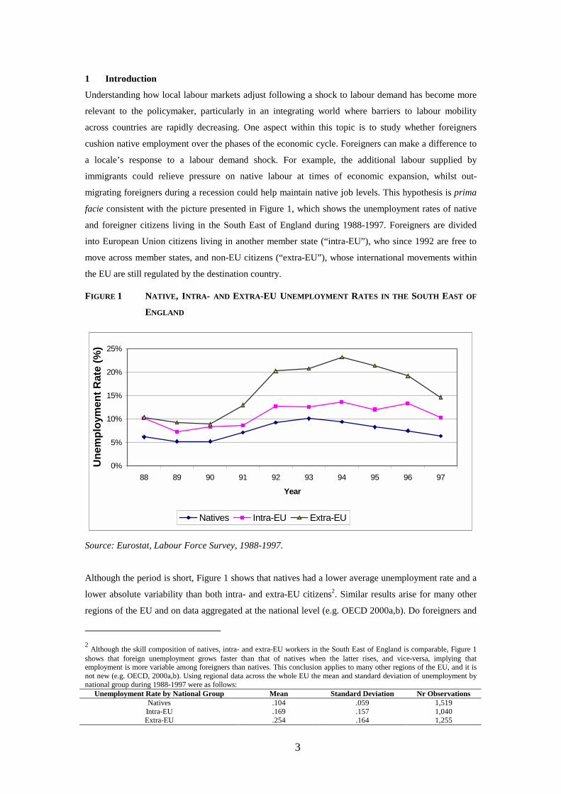
facie consistent with the picture presented in Figure 1, which shows the unemployment rates of native
and foreigner citizens living in the South East of England during 1988-1997. Foreigners are divided
into European Union citizens living in another member state (“intra-EU”), who since 1992 are free to
move across member states, and non-EU citizens (“extra-EU”), whose international movements within
the EU are still regulated by the destination country.
FIGURE 1 NATIVE, INTRA- AND EXTRA-EU UNEMPLOYMENT RATES IN THE SOUTH EAST OF
ENGLAND
0%
5%
10%
15%
20%
25%
88 89 90 91 92 93 94 95 96 97
Year
Une
mpl
oym
ent R
ate
(%)
Natives Intra-EU Extra-EU
Source: Eurostat, Labour Force Survey, 1988-1997.
Although the period is short, Figure 1 shows that natives had a lower average unemployment rate and a
lower absolute variability than both intra- and extra-EU citizens2. Similar results arise for many other
regions of the EU and on data aggregated at the national level (e.g. OECD 2000a,b). Do foreigners and
2 Although the skill composition of natives, intra- and extra-EU workers in the South East of England is comparable, Figure 1 shows that foreign unemployment grows faster than that of natives when the latter rises, and vice-versa, implying that employment is more variable among foreigners than natives. This conclusion applies to many other regions of the EU, and it is not new (e.g. OECD, 2000a,b). Using regional data across the whole EU the mean and standard deviation of unemployment by national group during 1988-1997 were as follows:
Unemployment Rate by National Group Mean Standard Deviation Nr Observations Natives .104 .059 1,519 Intra-EU .169 .157 1,040 Extra-EU .254 .164 1,255
4
hence policies favouring international migration, affect the level or the variability of native
employment?
This paper develops a theoretical model to address this question and presents some empirical results
using European regional data from Eurostat’s Labour Force Survey (LFS) for the period 1988-1997.
The paper is organised as follows. Section 2 briefly reviews the reference literature whilst section 3
develops a theoretical model. Section 4 presents the statistical model and the data used in the empirical
analysis, which is discussed in section 5. Section 6 concludes.
2 Foreign Workers and Local Labour Markets: A Brief Literature Review
The literature studying the effects of foreigners on native labour can be broadly divided in two. The
first group of studies focuses on individuals and it analyses the impact of immigrants on wages and
employment of native workers. These studies estimate functional models such as:
∆log wjit = ∆(F/N)it + ∆control variables (1)
where w refers to the wages of native person j in region i at time t, F and N indicate the number of
foreigners and natives in the same region and year, respectively. Equation (1) is generally estimated as
a pooled cross-section using data from censuses.
This literature finds small negative effects on wages and even smaller effects on employment (e.g.
Simon, 1989; Borjas, 1994). There are only few empirical studies based on European data3, which tend
to yield similar results (e.g. De New and Zimmermann, 1994; Dolado, Jimeno and Duce, 1996;
Gavosto, Venturini and Villosio, 1999).
As these studies estimate average individual responses to an inflow of immigrants, they focus on
specific aspects of a labour market’s reaction (e.g. change in wages or employment levels) rather its
overall response. However, they use the term migrant to mean either a foreign-born or an individual
holding a different citizenship from that of the country of residence, which is the definition applied in
this paper to purposely measure the labour market effect of international migrants.
In contrast, the second group of studies focuses on geographic areas and it often uses dynamic models
to estimate the impulse response function of a local labour market following a labour demand shock.
Many studies decompose the local labour markets’ response into changes in local employment and
participation rates, and in the working population4 exploiting the identity:
∆logEit = ∆log(E/L)it + ∆log(L/WP)it + ∆logWPit (2)
3 In the context of European migration, the few existing empirical studies reflect partly a limitation in the availability of data (particularly EU-wide data with comparable definitions across member states) and partly the characteristics of European labour markets. Across the EU the wage structure tends to be more rigid as it is often bargained and set nationally by unions. As a result, the impact of foreign immigration on wages is a priori expected to be limited (e.g. Pischke and Velling, 1996). 4 This is always true if the variables in (2) are measured in physical bodies (e.g. a rise in employment implies a change in the number of people). If the dependent variable is measured in efficiency units it is necessary to assume that the number of hours of labour supplied by each person is fixed.

5
where E is the number of employed in region i at time t, E/L is the employment rate, L/WP is the
participation rate and WP is the working population of the same region. Since most of the changes in
the working population are due to in- and out-migration rather than demographics, ∆logWP is typically
interpreted as a migration term.
US-based studies in this literature find that about two thirds of all jobs created in a locale go to
immigrants (see Bartik, 1993 for a summary). European studies reach mixed conclusions. At the
country level migration seems to be the principal adjustment mechanism through which a shock is
absorbed (Spain: Jimeno and Bentolila, 1998; Sweden: Fredriksson, 1999). In contrast, at the EU level
the shock seems to be mostly absorbed by changes in the participation rate and only later in time (3-4
years) by migration (Decressin and Fatas, 1995), though these results have been recently revisited
(Tani, 2003).
Although these studies use the unit of measure applied in this paper (regions), they use the word
migrant as a synonymous for newcomer with no distinction between a native from the same country or
someone born abroad. As a result, domestic and international migrants are indistinguishable, making it
impossible to carry out any analysis on the basis of citizenship. Nevertheless, the distinction between
native and foreign labour can be easily introduced in the theoretical framework of this literature, as
shown below.
3 A Theoretical Model of Local Labour Markets with Foreign Workers
The model developed in this section is based on the work of Blanchard and Katz (1992) but it departs
from it because it explicitly models labour supplied by people with different nationalities. Labour can
be supplied by either natives or foreigners from within (intra-EU) or outside the EU (extra-EU), who
differ only with respect to their wage elasticity of labour supply. By assumption natives supply labour
less elastically than foreigners as they may:
! have a more specific human capital than foreigners, or are more informed on available
employment opportunities, that better meets the demand of local firms (e.g. Chiswick, 1978);
! have better access to unemployment benefits and social security than foreigners, or native workers
may have been employed for a longer period of time than foreigners, so that foreign labour would
be cheaper to hire when firms raise employment and vice-versa (e.g. Chiswick and Hurst, 1996).
! not maximise their income potential for the skills they possess as they may face higher marginal
costs of migration than foreigners (e.g. Borjas, 2001).
There is some empirical evidence that immigrants supply labour more elastically than natives (e.g.
Borjas, 20015).
The remaining features of Blanchard and Katz (1992) are unchanged. The model represents a world
(the EU) composed of several regions, each producing a different bundle of goods under a constant
returns to scale technology. Labour and firms are perfectly mobile across regions in the long run, and
5 e.g. Borjas (2001) estimates the relative labour supply elasticity of new immigrants relative to natives is 1.3.

6
their mobility depends in part on the ‘attractiveness’ exerted by each region. Attractiveness is used in a
very general sense and includes all those characteristics that make labour and firms willing to locate in
a particular place. Hence, even with equal relative wages, regions can experience different net inflows
of labourers and firms because of their specific attractiveness.
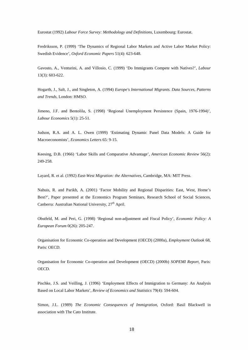
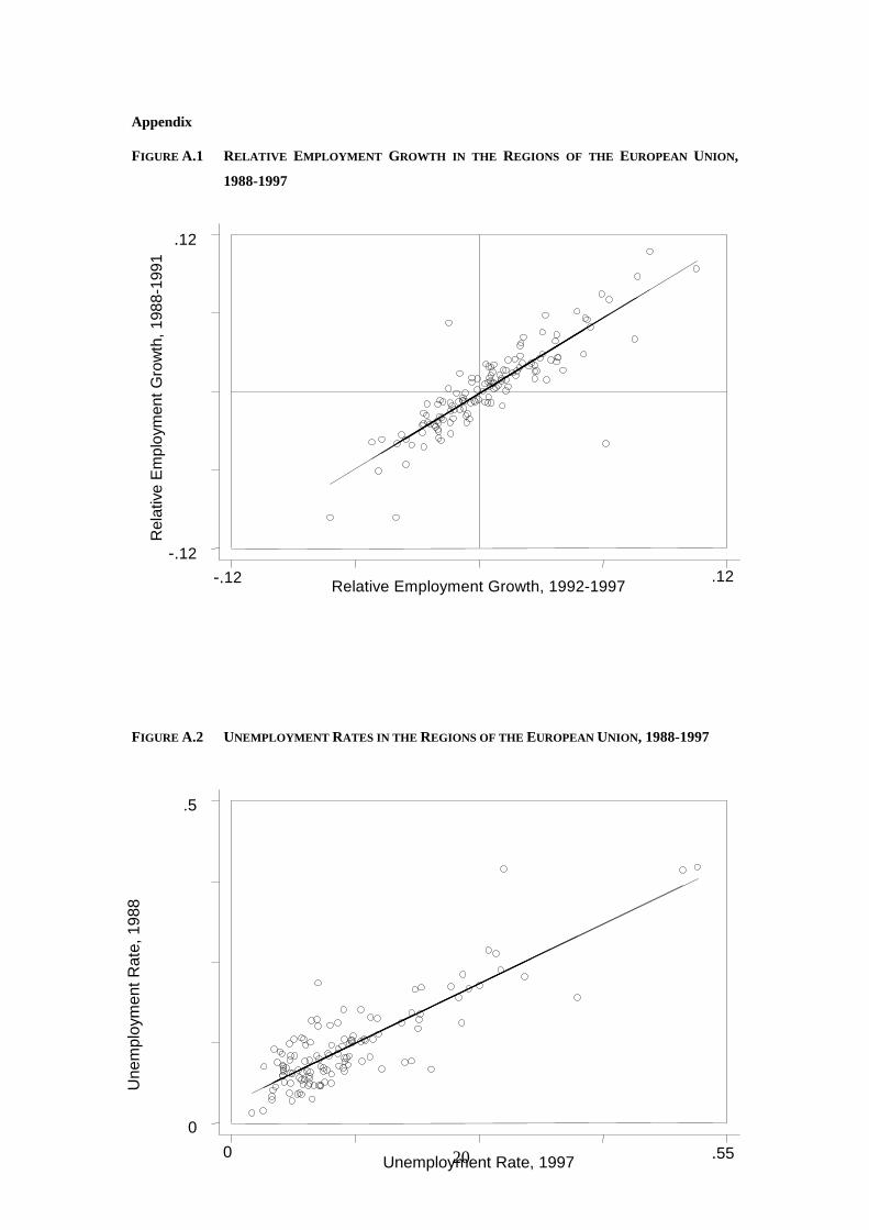
All variables in the model are measured relative to the EU average to identify regional labour demand
shocks, which are modelled as deviation from EU trends. This approach has been used by the literature
to capture remarkable empirical regularities in relative regional employment and unemployment in the
EU (see Figures A.1 and A.2 in the Appendix, as well as Decressin and Fatas, 1995).
Labour Demand
As in Blanchard and Katz (1992), the labour demand in each region i at time t is:
wit = – d(nit – uit) + zit (3)
where wit is the logarithm of region i’s wage relative to the average wage across the EU. The parameter
nit is the logarithm of the regional labour force, which is composed of both natives and foreigners,
relative to that at the EU level. The term uit is region i’s relative unemployment rate, which is defined
as:
uit = Uit/Eit (4)
where Uit and Eit represent region i’s total number of unemployed and employed (i.e. native plus
foreigners), respectively, at time t. This definition of unemployment is useful so that the difference (nit
– uit) in (3) is approximately equal to the logarithm of employment6. The coefficient d is assumed to be
positive.
The variable zit denotes the relative number of firms in region i and is defined as:
zit+1 – zit = – a wit + Xdi + εd
it+1|Ωt (5)
where a is a positive parameter, Xdi is the attractiveness of region i to firms, which is assumed to be
constant over time, and εdit+1 is a white noise stochastic process which represents unexpected changes
in technology, the bundle of goods produced and their relative prices. The superscript d of Xdi and εd
it+1
indicates ‘demand’, whilst Ωt is the information set at time t. By assumption firms do not have different
demands for native and foreign labour.
Since regions can differ in attractiveness to firms they can experience different rates of growth in
relative labour demand. Labour demand movements are also stochastic: as long as regional wages are
below their regional long-run equilibrium level firms will move in.
6 If U, E and N denote the numbers of unemployed, employed and those in the labour force, then u = U/E ≈ ln (1 + U/E) = ln(N) – ln(E). Hence (n – u) ≈ ln(N) – ln(N) + ln(E) = ln(E).
7
Labour Supply
A region’s labour supply is obtained by adding up those of its native and foreign residents. For
simplicity it is assumed that all nationalities can move freely across regions and member states7.
Changes in native and foreign labour supply are formalised by:
∆NLit = b1 wit + Xsi – guit + εs
1it+1|Ωt (6a)
∆FLit = b2 wit + Xsi – guit + εs
2it+1|Ωt (6b)
where ∆NLit is the growth of the native labour force in region i at time t, and ∆FLit is the corresponding
growth in the foreign labour force; wit and uit are defined as in (3); b1 is the labour supply elasticity
with respect to wages of natives, whilst b2 is the corresponding measure for foreigners; Xsi denotes
attractiveness to workers (e.g. local amenities), which is assumed to be identical for all citizens, and
time-invariant. The coefficient g denotes the sensitivity of native and foreign labour supply to region
i’s relative unemployment rate8. εsit+1 is a white noise stochastic component reflecting unexpected
changes in labour supply, e.g. a change in migration laws. The superscript s in Xsi and in the error terms
in (6a) and (6b) indicates ‘supply’. By assumption b2 is larger than b1, implying that foreign citizens
supply labour more elastically than natives.
The change in a region’s relative labour force is the weighted average of that of its native and foreign
residents, and it follows:
∆nit = (1 – θit)∆NLit + θit∆FLit (7)
where θit is the proportion of foreigners in region i’s labour force at time t, which can only vary
between zero and one (included). Short-term movements along the labour supply curves depend
negatively on the relative wage and positively on the relative unemployment rate. For a given the level
of attractiveness Xsi, as long as a region’s relative wage is below its long-run level native and foreign
labour out-migrate. Since workers and firms are assumed to be perfectly mobile in the long run there
exists a stable structure of relative unemployment and wage differentials across regions even when
employment growth rates differ across regions.
To close the model, the relative wage is assumed to be a function of unemployment9:
wit = – (1/c)uit (8)
where c is a positive parameter.
7 Although the movements of extra-EU workers throughout member states are regulated (the elimination of the restrictions to free movements within the EU provided by the Single European Act of 1986 do not apply to extra-EU workers), they are not impossible. 8 Allowing for different parameters for native and foreign labour groups does not modify the general prediction of the model, and results in a more complicated expression for the equilibrium conditions. Hence it is not discussed further. 9 As mentioned in Fredriksson (1999), “ this relationship is best thought of as relating the regional wage (in absolute terms) positively to the national wage rate, and negatively to the national and regional jobless rate respectively. Such a wage-setting schedule may result from national wage bargaining with additional wage drift at the firm level, given that the wage drift depends on labour market conditions in the particular region” (p.628). See also Blanchflower and Oswald (1994) for a discussion on the negative relationship between wages and the unemployment rate.
8
Equilibrium Paths and Steady States
The equilibrium paths of region i’s relative wage, unemployment rate, and labour force growth are
derived from the intersection of relative labour demand and supply curves (the results are in the
Appendix). Natives and foreigners face identical equilibrium paths with respect to the relative wage
and the unemployment rate. These are respectively:
w*it+1 = (1 + dc)-1[(1 + dc – dξit – dcg – a)wit + Xdi – dXs
i + εdit+1 – dεs
it+1|Ωt] (9)
u*it+1 = (1 + dc)-1[(1 + dc – dξit – dcg – a)uit – c(Xdi – dXs
i) – c(εdit+1|Ωt – dεs
it+1|Ωt)] (10)
In equations (9) and (10) the term ξit is a shorthand for expression ((1 – θit)b1 + θitb2), which increases
with rising shares of foreigners in the labour force, i.e. ∂ξit/∂θit > 0.
In contrast, natives and foreigners face different equilibrium paths with respect to the labour force
growth, as they have different labour supply functions. In particular region i’s native labour force
changes according to:
∆NL*it+1 = (1 + dc)-1(1 + dc – dξit – dcg – a)∆NLit + (b1 + gc)(Xdi + εd
it+1|Ωt) + (dξit + a – db1)Xsi
– (1 + dc – dξit – a + db1)εsit+1|Ωt + εs
it+2|Ωt (11)
By virtue of (4), the equilibrium path of native employment growth is approximately equal to the
difference (∆NLit+1 - ∆uit+1), i.e.:
∆NE*it+1 = (1 + dc)-1(1 + dc – dξit – dcg – a)∆NEit + d∆ξituit-1 + (b1 + gc)Xdi + (dξit + a – db1)Xs
i
+ (b1 + gc + c)εdit+1|Ωt – cdεd
it|Ωt – (1 + 2dc – dξit – a + db1)εsit+1|Ωt + cdεs
it|Ωt+
εsit+2|Ωt (12)
where NE stands for native employment. The equilibrium paths of native labour force and employment
growths are unique in each region, though they can vary across them.
The steady states of region i’s relative wage, unemployment rate, native labour force and employment
growth are obtained by solving expressions (9), (10), (11) and (12) for the average values of each
variable (see the Appendix). As in Blanchard-Katz (1992), the attractiveness of regions to workers and
firms (i.e. Xdi and Xs
i) are two underlying sources of regional employment growth. An increase in the
attractiveness to workers reduces the regional relative wage and the growth rates of the local labour
force and employment, whilst it increases the region’s relative unemployment rate. An increase in
attractiveness to firms increases the relative wage, the local labour force and employment and
decreases the relative unemployment rate. However, in the model presented here there is a third source
of employment growth: the share of foreigners in the local labour force. An increase in the proportion
of foreigners in the region reduces the steady state levels of regional wages, native labour force and
employment growth, whilst it raises the steady state of the unemployment rate, and vice-versa.
9
A One-off Shock to Labour Demand
Similar to Blanchard and Katz (1992), the effect of a one-off shock in relative labour demand is
transitory with respect to relative wage and unemployment but it is permanent on the level of relative
native labour force, as the labour force level series is assumed to contain a unit root10. This assumption
implies that any permanent change in the labour force results in an identical permanent change in the
employment level. The effect of a labour demand shock on the growth of the native labour force and
employment is therefore identical and it is equal to:
∂∆NLit+j+1/∂εdit|Ωt = ∂∆NEit+j+1/∂εd
it|Ωt = Σ ∞j=0 λj [(b1 + cg)/(1 + dc)] (13)
where λ = (1 + dc – dξit – dcg – a)/(1 + dc). As |λ| < 1, Σ ∞j=0 λj → 0 as j → ∞, implying that the long
run effect of a labour demand shock on both native labour force and employment growth is only
temporary.
In contrast, the shock has a permanent effect on the level of native labour force and employment, as
shown by:
∂NLit+j+1/∂εdit|Ωt = ∂NEit+j+1/∂εd
it|Ωt = (1 - λ)-1Σ ∞j=01j – λ(1 - λ)-1Σ ∞
j=0λj [(b1 + cg)/ (dξit + dcg
+ a)] (14)
Expression (14) tends to (b1 + cg)/ (dξt + dcg + a) ≠ 0 as j → ∞. In particular, since ξit is an increasing
function of θit, the long run effect of a shock on the native labour force and employment level is
inversely related to the proportion of foreigners in region i’s labour force. The higher the share of
foreigners in the local labour force, the smaller the permanent effect of a labour demand shock on
native labour and employment levels, and vice-versa. This result suggests that foreigners act as a
‘cushion’ to native employment, reducing its variability during the phases of the economic cycle. This
hypothesis can be easily verified empirically by testing the sign of the coefficient dξit/(1 + dc), which
appears identically in equations (11) and (12).
4 Methodology
4.1 Estimation Issues and Strategy Undertaken
The empirical analysis focuses on the sign of dξit/(1 + dc), which is estimated using equation (11) since
it has a simpler structure than equation (12). Equation (11) can be re-written as the statistical model11:
10 This assumption forces migration to explain permanent changes in employment level, and it is an important limitation as it may overestimate the role played by migration. Although this assumption is based on empirical findings for the US (Blanchard and Katz, 1992) and Europe (Decressin and Fatas, 1995), the Dickey-Fuller test on unit roots yields mixed results. The prior of a unit root in employment growth is rejected by over half of the sample (e.g. Decressin and Fatas, 1995; Fredriksson, 1999), but the prior is maintained on the basis of the low power of the test due to the short time series. However, when the model is modified to accommodate a stationary relative employment (Obstfeld and Peri, 1998), imposing the long-run effects of labour demand shocks on migration to be zero, “the first year effects and the response five years out are very close to those [of Blanchard and Katz (1992)]” (p.228). In this paper re-running the model on the series on employment level yields broadly similar results to those obtained when the series on employment growth. The Dickey-Fuller test is rejected by over half of the sample but the prior that the series contains a unit root is maintained on the basis of the low power of the test caused by the short time of the series (nine years). 11 In particular: β = (1 + dc)-1(1 + dc – dcg – a – db1); γ = (1 + dc)-1 d(b1 – b2); δ = (1 + dc)-1(b1 + gc); µ = a (1 + dc)-1; χ = (1 + dc)-1d(b2 – b1)Xs
i; and νit is an error term that is assumed to be uncorrelated with present and past values of the explanatory
10
∆NL*it+1 = β∆NLit + γθit∆NLit + δXdi + µXs
i + χθit + νit (15)
Under the assumption that b2 > b1, the coefficient γ = (1 + dc)-1d(b1 – b2) is negative, implying that the
evolution of native labour force and employment are smoother in regions with higher proportions of
foreigners in the local labour force, and vice-versa.
It is natural to think of estimating equation (15) with panel data techniques to exploit the longitudinal
feature of the data, and to eliminate the likely presence of regional fixed unobserved variables. In doing
so, one has to bear in mind that the variables Xdi and Xs
i, which were assumed to be regional time-
invariant constants, will also be eliminated in the estimation process12.
Since the lagged value of the dependent variable appears on the right hand side of (15), the explanatory
variables are not all strictly exogenous. Hence, the estimation through fixed effects, random effects and
first differencing will generally produce inconsistent estimates (e.g. Wooldridge, 1999). Inconsistency
can be serious if the number of observational units is far larger than the fixed number of years for
which data are available, as it is in this paper (Judson and Owen, 1999). Consistent estimates for
equation (15) can however be obtained through a generalised method of moments procedure, where the
explanatory variables are first transformed to eliminate unobservable regional fixed effects, and then
estimated by instrumental variables. In particular this paper applies the dynamic panel data estimator
developed by Arellano and Bond (1991), which instruments the endogenous variables with the lagged
levels of dependent and predetermined variables and the differences of strictly exogenous variables. In
the transformed equation, ∆NLit is instrumented by its lagged values up to ∆NLit-2. This methodology
relies on the testable assumption that the first difference of the residuals does not follow a second-order
autocorrelation process (Wooldridge, 1999; Stata, 2001).
To obtain a labour force growth time series reflecting only labour demand shocks, the dependent
variable in equation (15) is transformed using the method applied by Blanchard and Katz (1992) and
the subsequent literature. This method assumes that any innovation in region i’s relative labour force
growth is a local labour demand shock. As a result, the dependent variable in equation (15) is ‘purged’
of EU disturbances by first estimating common movements across regions using:
∆logNit = αi + βi ∆logNEUt + ϕit (16)
where Nit is the number of natives in the labour force of region i at time t, NEUt is the corresponding EU
average, and ϕit is an error term. Then the dependent variable is transformed into its regional relative
equivalent by removing the common movements estimated from (16), using:
NLit = logNit - βi logNEUt (17)
where Nit and NEUt are defined as in (16) and βi is the estimate obtained from (16).
variables. This assumption is formally tested in the empirical analysis. 12 As Xs
i is time-invariant, it was incorporated into the parameter χ (= -γXs) rather than being treated as an independent variable.
11
4.2 The Data
Equation (15) is estimated on a panel consisting of 161 regions of 12 member states of the EU covering
the period 1988-1997. The data are extracted from Eurostat’s Labour Force Survey (LFS), a household
survey that collects data on population stocks across the whole EU using internationally comparable
definitions and methodology (see Eurostat, 1992). This feature makes the LFS an ideal data source for
cross-country studies on international migration in the EU (e.g. Angrist and Kugler, 2001; Nahuis and
Parikh, 2001).
The panel contains data on the regional stocks of labour by nationality as well as demographic and
labour market data. The regions correspond to the administrative level immediately below that of the
country (NUTS 2). The panel is unbalanced, and complete data are available for 128 regions13.
Adjustments were made to maintain the geographic consistency of the sample as regional boundaries (and
country boundaries in the case of Germany) have sometimes changed during the period14. Missing
observations were filled in the case of Italy, where the nationality of the labour force for the years 1988-
1991 was inferred from the aggregate data, using the average share of foreign labour during 1992-1997.
The employment data in the panel are restricted to employees aged 25 and above. Table 1 presents a
statistical summary of the variables used in the empirical analysis, separating those that are explicitly
modelled in equation (15) (dependent/independent) from those used as a control (control - labour
market and control - demographics). Control variables refer mostly to natives to match the unit of
measure of the dependent variable. Except for the share of foreigners in the labour force, the other
variables used in the regression are transformed into their relative regional equivalent following the
methodology applied in equations (16) and (17).
TABLE 1 SUMMARY STATISTICS OF VARIABLES USED
Variable Observations Mean STD 10th
Dec.
90th
Dec.
Dependent/Independent
Labour Force Growth (natives) 1,337 .0121 .0339 -.024 .049
Share of foreigners in the labour force 1,337 .0463 .0458 .002 .125
Control – Labour market
Skilled/unskilled ratio (natives) 1,326 2.328 1.064 1.34 4.18
Share of firms with 50+ employees* 945 .3895 .2001 .001 .518
Share of agricultural employment (natives)* 945 .0354 .0603 .011 .120
Control – Demographics
Male/female ratio (natives) 1,337 1.276 .4179 1.07 2.00
13 Data for Italy (20 region) and the former East Germany (7 regions) by nationality are available only since 1992 and 1991, respectively. 14 The most important changes regard Belgium (where the regions of Nivelles and Limburg are recorded separately until 1995 but not afterwards) and Germany (the distinction in East and West Berlin has been eliminated in 1995. Since then, the regions of Chemnitz, Dresden, and Halle have also been combined in a single region). As a result, regions recorded individually and then merged have been combined together also during the years prior to 1995.
12
Share of employees aged 25-34 (natives) 1,337 .4111 .0375 .361 .459
* = Data available only for the period 1992-1997.
The first row of Table 1 summarises the native labour force growth across the EU. There is significant
variability across both time and regions: the period examined roughly covers an economic cycle, with
regional employment levels in 1997 only slightly higher than in 1988, whilst the extreme values of the
variable generally refer to less densely populated regions and islands15.
The statistics in the second row of Table 1 show that foreigners in the EU are a small percentage of the
labour force compared with other OECD countries (e.g. OECD, 2000a,b). Foreign citizens are nil in
several regions of the sample16, though they are a non-negligible group in member states that have
traditionally experienced positive net immigration rates (Germany, France, Benelux, and Denmark).
The data indicate that foreigners in the EU are mainly non-recent immigrants, as the proportion of
those with 10 or more years of residence in the host country17 is well over 50%. There is significant
regional variation is the value of this ratio, which is lowest in regions that have experienced net
immigration rates only since the 1980s (Spain, Italy, Greece, Portugal, and Ireland) and highest in
traditional destination countries.
The control variables aim at capturing labour market and demographic characteristics. Among the former,
the ratio of skilled/unskilled native labour is constructed using the aggregation of occupations
suggested by Keesing (1966). Some control variables are available only since 1992, following a
substantial restructuring and extension of the LFS questionnaire. Despite this administrative change,
the Chow test on structural break on the data used in the empirical analysis is rejected, suggesting that
the pre- and post-1992 series are comparable. Year dummy variables are included in the estimation to
control for possible annual measurement errors in the LFS (e.g. national biases in data collection),
though the results are unaffected when the year dummies are omitted.
15 e.g. Valle d’Aosta, Marche (Italy), Poitou-Charentes, Languedoc, Auvergne, Corsica (France), Western Macedonia, Aegean Islands, Crete, Peloponnisos (Greece), Ceuta and Melilla (Spain), Alentejo, Algarve (Portugal), Mid-West, North East (Ireland). 16 This occurs as the LFS data capture mainly legal labour. Foreign immigrants are likely to be under-represented in the LFS as it is a household-based survey, which excludes many types of accommodation where foreign immigrants are likely to live (e.g. hostels). See Hogarth, Salt, and Singleton (1994) for a comprehensive discussion of issues related to measuring immigration in the EU. 17 The mean value of this variable is 56.4% and its standard deviation is 15.37%. Although there are 757 observations for which this variable is available in the sample, it is excluded from the estimation of equation (15) as it is not available for all countries throughout the period examined (e.g. it is available for Germany only for 1992).
13
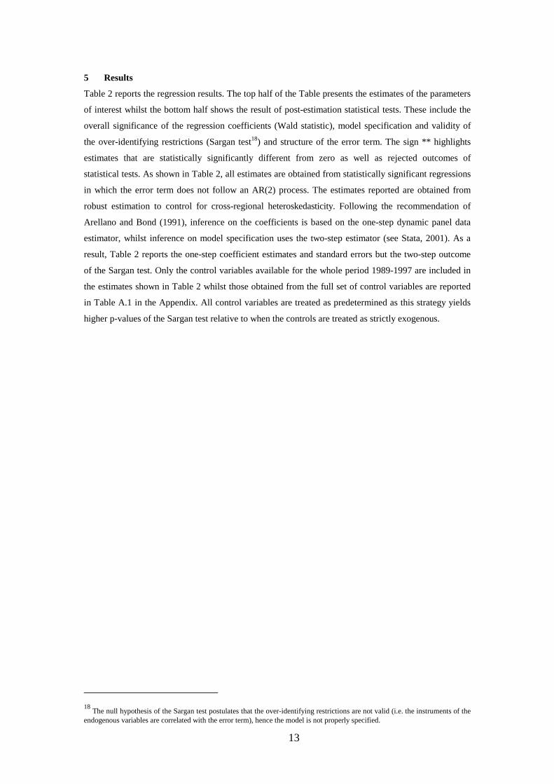
5 Results
Table 2 reports the regression results. The top half of the Table presents the estimates of the parameters
of interest whilst the bottom half shows the result of post-estimation statistical tests. These include the
overall significance of the regression coefficients (Wald statistic), model specification and validity of
the over-identifying restrictions (Sargan test18) and structure of the error term. The sign ** highlights
estimates that are statistically significantly different from zero as well as rejected outcomes of
statistical tests. As shown in Table 2, all estimates are obtained from statistically significant regressions
in which the error term does not follow an AR(2) process. The estimates reported are obtained from
robust estimation to control for cross-regional heteroskedasticity. Following the recommendation of
Arellano and Bond (1991), inference on the coefficients is based on the one-step dynamic panel data
estimator, whilst inference on model specification uses the two-step estimator (see Stata, 2001). As a
result, Table 2 reports the one-step coefficient estimates and standard errors but the two-step outcome
of the Sargan test. Only the control variables available for the whole period 1989-1997 are included in
the estimates shown in Table 2 whilst those obtained from the full set of control variables are reported
in Table A.1 in the Appendix. All control variables are treated as predetermined as this strategy yields
higher p-values of the Sargan test relative to when the controls are treated as strictly exogenous.
18 The null hypothesis of the Sargan test postulates that the over-identifying restrictions are not valid (i.e. the instruments of the endogenous variables are correlated with the error term), hence the model is not properly specified.
14
TABLE 2 REGRESSION RESULTS, 1989-1997
Coefficient 161 EU
Regions
161 EU
Regions
Traditional
Immigration
Regions
Recent
Immigration
Regions
β .103
(.101)
.093
(.091)
.065
(.124)
.016
(.090)
γ -1.357*
(.788)
-1.612**
(.825)
-3.380*
(1.783)
-15.756**
(4.781)
χ -.885**
(.398)
-.870**
(.439)
-1.102**
(.450)
.967
(.661)
Constant -.0001
(.001)
.00005
(.001)
-.001
(.002)
.002
(.002)
Nr Observations
1,014 1,014 640 374
Control variables
Year Dummies Yes Yes Yes Yes
Regional labour marketa No Yes Yes Yes
Regional demographicsa No Yes Yes Yes
Tests
Wald test of overall
significance
74.09** 61.76** 99.24** 45.83**
Serial AR(2) in the error
term
p = .7195 p = .6389 p = .6716 p = .0661
Sargan test (based on the
two-step estimator)
p = .0007** p = .2776 p = .9993 p = .7315
a = includes only the control variables available for the whole period 1989-1997.
The first and second columns in Table 2 report the results when equation (15) is estimated without and
with control variables, respectively. The discussion focuses on the results shown in the second column,
as the regression is better specified when control variables are included, as show by the Sargan test,
which fails to be rejected.
The estimates obtained show that γ has a negative sign and is statistically significant, suggesting that
annual changes in a region’s native employment are inversely related to the proportion of foreign
citizens in that region’s labour force. In particular, following a labour demand shock, the higher is the
share of foreign labour the more foreigners absorb the year-after effects caused by the shock,
cushioning natives from its full impact. Over time the shield provided by foreign labour makes native
employment levels less variable, as predicted by the theoretical model presented in Section 3. The
15
negative sign of the coefficient γ is robust to model specification, and to estimation on subsets of the
panel, including the sub-periods prior and after 1992.
The magnitude of the cushioning effect is not insignificant. Foreign labour mitigates native
employment from the effects of a shock well above its share in the local labour force. Using the
estimate of γ = 1.612 (second row, second column), foreigners are predicted to reduce the variability of
native labour in a region by more than 8% when they constitute 5% of that region’s labour force.
This result varies across countries. In member states that have traditionally imported foreign labour, the
coefficient γ is negative but seldom statistically significant. The parameter γ is statistically significant
only at the 10% level when equation (15) is estimated on the pooled regions of traditional immigration
countries19 (third column in Table 2). Perhaps this outcome is not surprising. During the reconstruction
years that followed WWII until the early 1970s, most of these countries have systematically imported
foreigners to fill gaps in their native labour force, most notably in Germany (Böhning, 1984 and 1991;
Zimmermann, 1995). Between the mid-1970s and the late 1980s immigration came to a halt (except for
family reunification), whilst the recent upsurge includes many asylum seekers and refugees whom
cannot immediately enter the host country’s labour force. A significant shielding effect would almost
contradict these countries’ past immigration policies.
In contrast, in member states that have experienced net immigration rates only recently (Greece, Italy,
Spain, Portugal and Ireland), the term γ is always statistically significant and its magnitude is very
large. As shown in the fourth column of Table 2, the size of the coefficient γ in recent immigration
areas is a multiple of that reported in traditional immigration areas. This result may be due to the low
incidence of foreigners in the local labour force of these regions (less than 1%). An alternative
explanation is that foreigners in recent immigration regions are ‘newer’ and may have a higher
elasticity to supply labour than immigrants in traditional host countries. On the basis of the information
available in the panel, this hypothesis is supported20, though one should ideally investigate it using
microeconomic data.
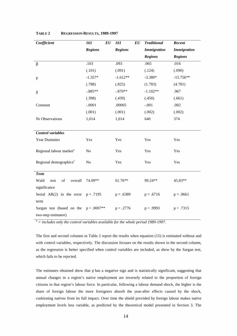
To further assess the results presented in Table 2, a simple calculation was performed whereby the
average composition of the labour force stock by nationality was compared with that of its changes
over the period 1988-199721. If foreigners shield native labour then they should be over-represented in
the measure of the changes relative to that of the stocks. The top half of Table 3 shows the results of
this calculation with respect to the labour force, whilst the bottom half of the Table shows the
analogous calculation performed on employment data.
19 This result is mainly due to the presence of French and Dutch regions. When these are excluded from the regression (or when the agricultural employment share control variable is included), the coefficient γ is still negative but no longer statistically significantly different from zero. 20 The average proportion of foreigners residing 10 or more years in the host country is 40% in Recent Immigration Regions vis-à-vis 62% in Traditional Immigration Regions. 21 I.e. ΣitLFit,foreign/ΣitLFit, (natives + foreigners) is compared to Σit∆LFit,foreign/Σit∆LFit, (natives + foreigners)
16
TABLE 3 LABOUR FORCE AND EMPLOYMENT COMPOSITION BY NATIONALITY ACROSS THE
EU, 1988-1997
Pooled Regions Traditional
Immigration Regions
Recent Immigration
Regions
Stock Change Stock Change Stock Change
LABOUR FORCE
Foreigners 4.63% 5.54% 6.75% 6.79% 0.75% 2.32%
Natives 95.37 94.46 93.25 93.21 99.25 97.68
EMPLOYMENT
Foreigners 4.54 3.91 6.20 4.06 0.70 3.13
Natives 95.46 96.09 93.80 95.94 99.30 96.87
Number of Cases 1,519 1,351 893 800 626 551
The measure in the top left corner of Table 3 (‘Pooled Regions - stock’) shows that during 1988-1997
foreigners were on average 4.63% of the labour force stock across the EU but constituted 5.54% of its
changes (‘Pooled Regions – Change’), implying that foreigners shield native labour during the
economic cycle. This outcome is only marginally supported in traditional immigration regions
(columns in the middle of Table 3), whilst it is remarkably strong in recent immigration regions,
providing additional support to the regression results discussed earlier.
With respect to employment, foreigners do not appear to cushion native jobs overall (bottom half of the
first column), as they constitute 4.54% of the regional employment stock but only 3.91% of its
changes. Foreigners are particularly under-represented in the measures of the employment change in
traditional immigration regions, which have traditionally experienced demand-driven immigration,
whilst they seem to shield native labour in recent immigration regions, as already emerged in the
regression results.
6 Conclusions
This paper shows that when foreigners have a higher wage elasticity to supply labour than natives, they
can reduce the variability of native labour growth and level as they absorb some of the impact of a
labour demand shock. The empirical results, based on macroeconomic data covering 161 EU regions
during 1988-1997, support this hypothesis.
17
References
Angrist, J.D. and Kugler, A.D. (2001) Immigration, Native Employment, and Labor Market Flexibility
in Western Europe (mimeo). Cambridge, MA: MIT Press.
Arellano, M. and Bond, S.R. (1991) ‘Some Specification tests for Panel Data: Monte Carlo Evidence
and an Application to Employment Equations’, Review of Economic Studies 58: 277-298.
Bartik, T.J. (1993) ‘Who Benefits from Local Job Growth: Migrants or the Original Residents?’,
Regional Studies 27(4): 297-311.
Blanchard, O.J. and Katz, L.F. (1992) ‘Regional Evolutions’, Brookings Papers on Economic Activity
0(1): 1-75.
Blanchflower, D.G. and Oswald, A.J. (1994) The Wage Curve, Cambridge, MA: MIT Press.
Böhning, W.R. (1984) Studies in International Labour Migration, London: Macmillan.
Böhning, W.R. (1991) ‘Integration and Immigration Pressures in Western Europe’. International
Labour Review 130(4): 445-458.
Borjas, G.J. (2001) ‘Does Immigration Grease the Wheels of the Labor Market?’, Brookings Papers on
Economic Activity 0(1): 69-119.
Chiswick, B.R. (1978) ‘The Effect of Americanization on the Earnings of Foreign-Born Men’, Journal
of Political Economy 86(5): 867-921.
Chiswick, B.R. and Hurst, M.E. (1996) ‘The Employment, Unemployment and Unemployment
Compensation Benefits of Immigrants’, Paper presented at the European Science Foundation
Conference on Migration and Development Policy, France, June.
Decressin, J. and Fatas, A. (1995) ‘Regional Labour Market Dynamics in Europe’, European Economic
Review 39: 627-1655.
De New, J.P. and Zimmermann, K.F. (1994) ‘Native Wage Impacts of Foreign Labor: A Random
Effects Panel Analysis’, Journal of Population Economics 7(2): 177-192.
Dolado, J.J., Jimeno, J.F., and Duce, R. (1996) The Effects of Migration on the Relative Demand of
Skilled versus Unskilled Labour: Evidence from Spain, Centre for Economic Policy Research
Discussion Paper 1476, London.
18
Eurostat (1992) Labour Force Survey: Methodology and Definitions, Luxembourg: Eurostat.
Fredriksson, P. (1999) ‘The Dynamics of Regional Labor Markets and Active Labor Market Policy:
Swedish Evidence’, Oxford Economic Papers 51(4): 623-648.
Gavosto, A., Venturini, A. and Villosio, C. (1999) ‘Do Immigrants Compete with Natives?’, Labour
13(3): 603-622.
Hogarth, J., Salt, J., and Singleton, A. (1994) Europe's International Migrants. Data Sources, Patterns
and Trends, London: HMSO.
Jimeno, J.F. and Bentolila, S. (1998) ‘Regional Unemployment Persistence (Spain, 1976-1994)’,
Labour Economics 5(1): 25-51.
Judson, R.A. and A. L. Owen (1999) ‘Estimating Dynamic Panel Data Models: A Guide for
Macroeconomists’, Economics Letters 65: 9-15.
Keesing, D.B. (1966) ‘Labor Skills and Comparative Advantage’, American Economic Review 56(2):
249-258.
Layard, R. et al. (1992) East-West Migration: the Alternatives, Cambridge, MA: MIT Press.
Nahuis, R. and Parikh, A. (2001) ‘Factor Mobility and Regional Disparities: East, West, Home’s
Best?’, Paper presented at the Economics Program Seminars, Research School of Social Sciences,
Canberra: Australian National University, 27th April.
Obstfeld, M. and Peri, G. (1998) ‘Regional non-adjustment and Fiscal Policy’, Economic Policy: A
European Forum 0(26): 205-247.
Organisation for Economic Co-operation and Development (OECD) (2000a), Employment Outlook 68,
Paris: OECD.
Organisation for Economic Co-operation and Development (OECD) (2000b) SOPEMI Report, Paris:
OECD.
Pischke, J.S. and Veilling, J. (1996) ‘Employment Effects of Immigration to Germany: An Analysis
Based on Local Labor Markets’, Review of Economics and Statistics 79(4): 594-604.
Simon, J.L. (1989) The Economic Consequences of Immigration, Oxford: Basil Blackwell in
association with The Cato Institute.

19
Stata Corporation (2001) Stata Statistical Software: Release 7.0, College Station, TX: Stata
Corporation.
Wooldridge, J.M. (1999) Econometric Analysis of Cross Section and Panel Data, Cambridge, MA: The
MIT Press.
Zimmermann, K.F. (1995) ‘European Migration: Push and Pull’ in M. Bruno and B. Pleskovic (Eds.),
Supplement to the World Bank Economic Review and the World Bank Research Observer, Washington,
DC: The World Bank.
*** (2003) ‘Have Europeans Become More Mobile? A Note on Regional Evolutions in the EU: 1988-
1997’, Economics Letters (forthcoming).
20
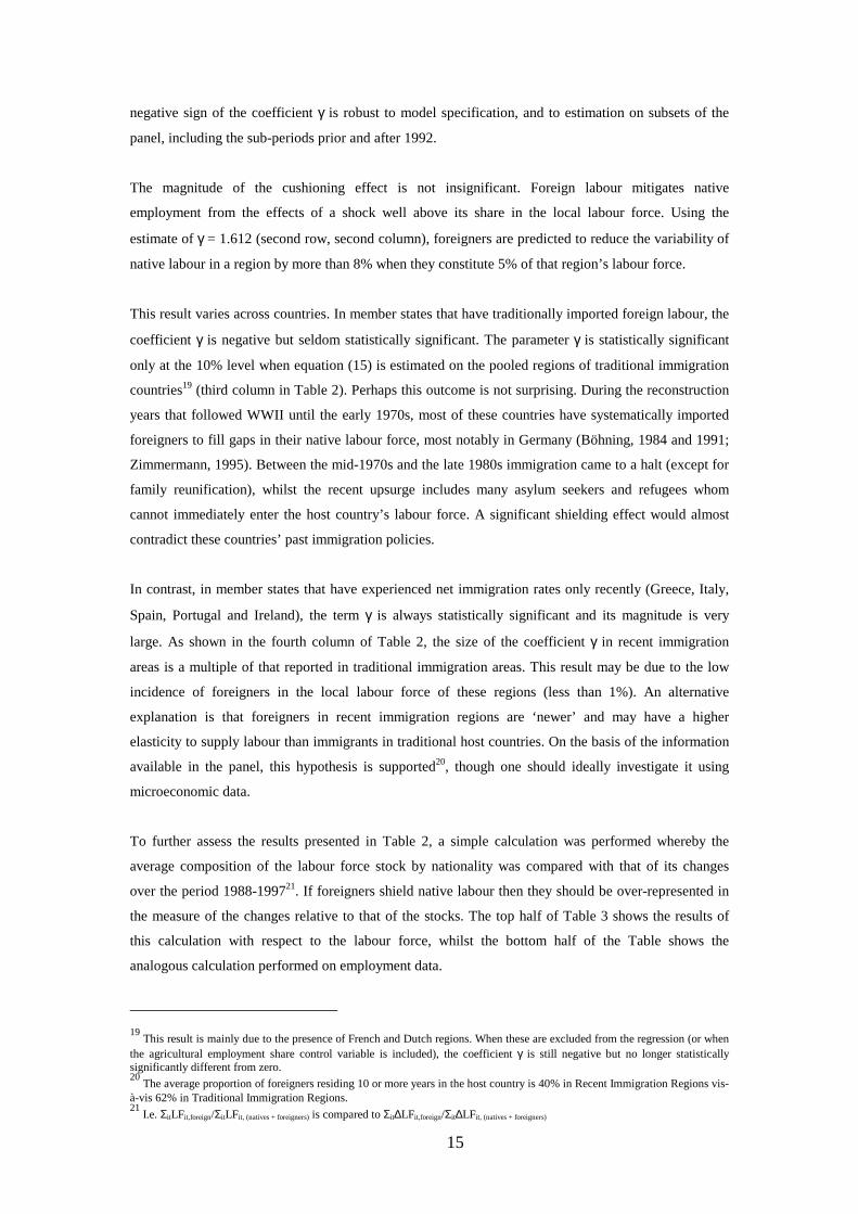
Appendix
FIGURE A.1 RELATIVE EMPLOYMENT GROWTH IN THE REGIONS OF THE EUROPEAN UNION,
1988-1997
FIGURE A.2 UNEMPLOYMENT RATES IN THE REGIONS OF THE EUROPEAN UNION, 1988-1997
Rel
ativ
e Em
ploy
men
t Gro
wth
, 198
8-19
91
Relative Employment Growth, 1992-1997-.12 .12-.12
.12
Une
mpl
oym
ent R
ate,
198
8
Unemployment Rate, 19970 .550
.5

21
A BRIEF SUMMARY OF THE THEORETICAL MODEL
Solving the Model
Substituting expressions (6a), (6b) and (8) in (7) yields:
∆nit = [(1 - θit)b1 + θitb2 + cg] wit + Xsi + εsit+1|Ωt (A.1)
whilst substituting expressions (A.1) and (5) in (3) yields:
(1 + dc)∆wit = [1 + dc – dξit – dcg – a]wit – dXsi + Xdi – dεsit+1|Ωt + εd
it+1|Ωt] (A.2)
In equilibrium, relative labour supply and demand are equal. This yields the restricted equation, consisting
of a system that solves for relative wages and employment growth. The equilibrium paths for relative
wage, unemployment, labour force and employment growth are:
w*it+1 = (1 + dc)-1[(1 + dc – dξit – dcg – a)wit + Xdi – dXs
i + εdit+1|Ωt – dεs
it+1|Ωt] (A.3a)
u*it+1 = (1 + dc)-1[(1 + dc – dξit – dcg – a)uit – c(Xdi – dXs
i) – c(εdit+1|Ωt – dεs
it+1|Ωt)]
(A.3b)
∆n*it+1 = [(1 + dc)(ξit + cg)]-1[(ξit+1 + cg)(1 + dc – dξit – dcg – a)]∆nit + (1 + dc)-1 (ξit+1 + cg) (Xdi +
εdit+1|Ωt) + [(1 + dc)(ξit + cg)]-1[(1 + dc)(ξit + cg) + (ξit+1 + cg)(a – 1 – dc)] Xs
i + [(1 + dc)(ξit +
cg)]-1[(ξit+1 + cg)(a – 1 – dc)]εsit+1 + εs
it+2|Ωt (A.3c)
Solving (A.3a) and (A.3b) with respect to wages yields:
wit+j+1 = Σ∞j=0 [(1 + dc – dξit – dcg – a)/(1 + dc)]j * (1 + dc)-1 [Xdi – dXsi – dεs
it+1|Ωt + εdit+1|Ωt]
(A.4)
The effect of a shock on wages is:
∂wit+j+1/∂εdit|Ωt = [(1 + dc – dξit – dcg – a)/(1 + dc)]j (1 + dc)-1 (A.5)
which tends to zero as j → ∞ because the term inside the square bracket is smaller than one.
The effect of a shock on the unemployment rate is ∂uit+j/∂εdit+1|Ωt = – c ∂wit+j+1/∂εd
it|Ωt which also tends to
zero as j → ∞.
The effect of a shock on the aggregate labour force (hence employment) growth is:
∂∆nit+j+1/∂εdit|Ωt = ((1 – θit+1)b1 + θit+1b2 + cg) ∂wit+j+1/∂εd
it|Ωt (A.6)
which also tends to zero as j → ∞. However, the level of aggregate employment is permanently affected
as:
∂nit+j+1/∂εdit|Ωt = [(ξit + cg)(ξit+1 + cg)] / [(ξit – ξit+1)(1 + dc) + (ξit+1 + cg)(dξit + dcg + a)] ≠ 0
(A.7)
22
In particular:
∂NLit+j+1/∂εdit|Ωt = (b1 + cg) / [dξit + dcg + a] (A.8)
∂FLit+j+1/∂εdit|Ωi = (b2 + cg) / [dξit + dcg + a] (A.9)
The steady states of the relative wage, employment growth and unemployment rate for region i are
obtained by solving equations (A.3a), (A.3b) and (A.3c) for the average values of these variables. For
the natives, these steady states are respectively:
wi = (a + dξit + dcg)-1(Xdi – dXs
i) (A.11)
∆NLi = (a + dξit + dcg)-1 [(b1 + cg)Xdi + (a + dξit – db1)Xs
i] (A.12)
ui = (a + dξit + dcg)-1[– c(Xdi – dXs
i)] (A.13)
Foreign labour raises ξit and therefore reduces the steady state level of relative wages and relative
labour force and employment growth, but it raises that of relative unemployment.
Preliminary Tests of the Data
Tests on the Construction Region-Specific Variables
The OLS regression on (16) on employment by nationality indicates that on average less than a quarter
of yearly movements in labour force are common to all regions. In each case, a Chow test has been
performed to test the possibility of structural break in the data pre- and post-1992. The test failed to
reject the hypothesis of structural change between these two periods. In several instances, the
regression by region failed the F-test of overall significance. These cases yielded both insignificant
estimates of βi and significance of the regression, and are characterised by low or negative adjusted R-
squares. However, in virtually all cases, the RESET22 test of specification failed to reject the hypothesis
that equation (16) has no omitted variables. The density estimation of αi and βi across all regions show
that both parameters have a distribution similar to a normal with mean values of 1.419 and 0.611,
respectively. Hence the assumption of normality and the properties of large samples can be applied in
the estimation.
The cross-section regression (16) on all regions pooled together indicate the presence of
heteroskedasticity, which is tested using the Cook-Weisberg test23. However, when the regression (16)
is performed by region, the test fails to reject the null hypothesis of constant variance. Since the
construction of the region-specific variables is based on the results obtained in the latter case, the issue
of heteroskedasticity does not appear to be of concern.
22 If the functional form (16) is properly specified (i.e. there are no missing variables) then adding the fitted value of the dependent variable from (16) as an additional explanatory variable in an augmented version of (16) should not increase the significance of the model. 23 This heteroskedasticity test models the variance of the error term in (16) as σ2exp(zt) where z is a variable equal to the fitted values Xβ. The test is of t=0 (Stata, 2001).

23
The leverage analysis24 of the pooled regression indicates that in the case of employment growth the
French region of Corsica is a clear outlier, whilst in the cases of unemployment rate the extremes are
several Spanish, Portuguese, Greek and Italian regions. The models were re-estimated dropping these
observations. Since similar results were obtained, all regions are left in the working sample.
24 This analysis studies the graph of leverage (the weight of each observation in yielding the regression result) against the normalised residuals squared. This graph allows the researcher to identify observations which are outliers and have a significant impact on the regression results obtained, and it is used to better interpret the original data (Stata, 2001).
24
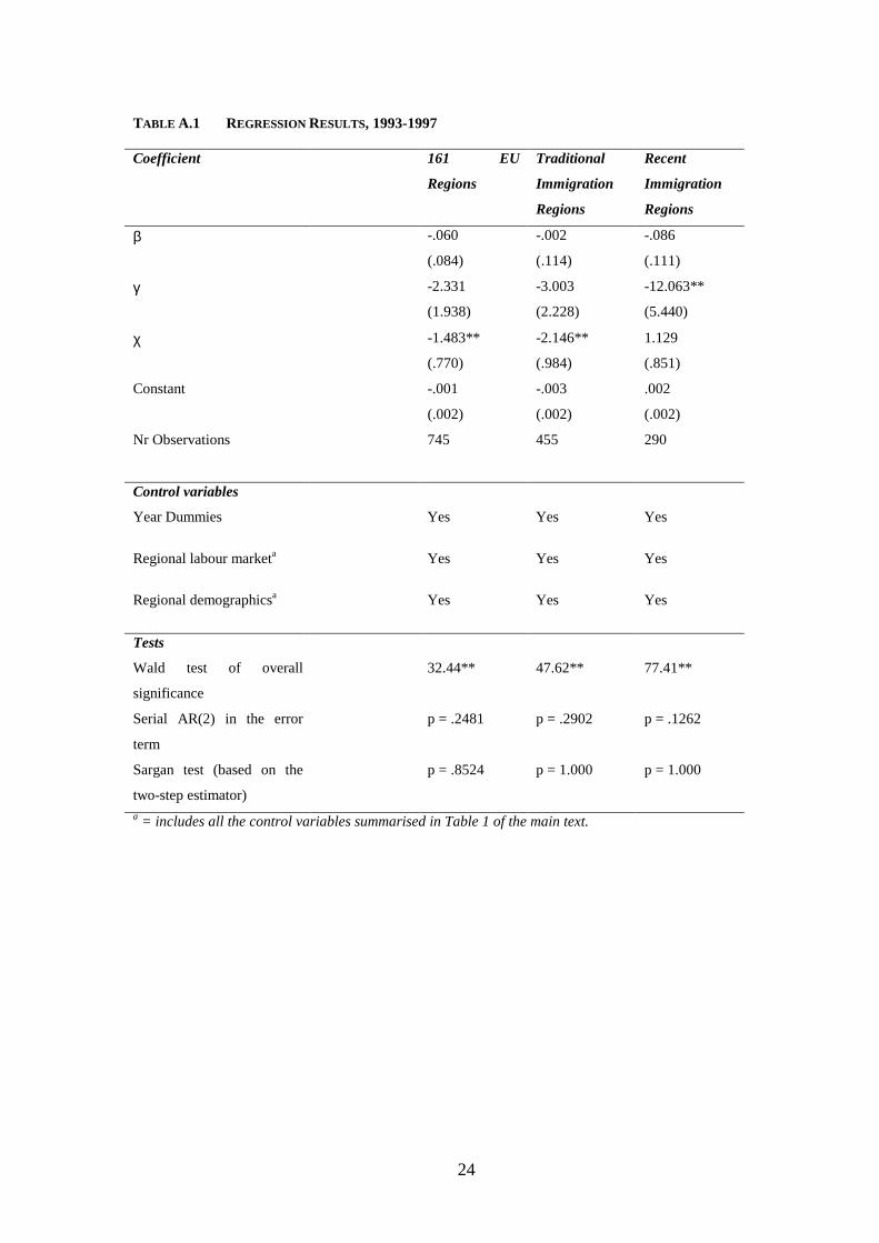
TABLE A.1 REGRESSION RESULTS, 1993-1997
Coefficient 161 EU
Regions
Traditional
Immigration
Regions
Recent
Immigration
Regions
β -.060
(.084)
-.002
(.114)
-.086
(.111)
γ -2.331
(1.938)
-3.003
(2.228)
-12.063**
(5.440)
χ -1.483**
(.770)
-2.146**
(.984)
1.129
(.851)
Constant -.001
(.002)
-.003
(.002)
.002
(.002)
Nr Observations
745 455 290
Control variables
Year Dummies Yes Yes Yes
Regional labour marketa Yes Yes Yes
Regional demographicsa Yes Yes Yes
Tests
Wald test of overall
significance
32.44** 47.62** 77.41**
Serial AR(2) in the error
term
p = .2481 p = .2902 p = .1262
Sargan test (based on the
two-step estimator)
p = .8524 p = 1.000 p = 1.000
a = includes all the control variables summarised in Table 1 of the main text.


![Untitled-1 [] · Cushion: M*2 Cushion: M*2 Cushion: M*1 Cushion: M*1 Cushion: M*2 Cushion: M*3 Cushion: M*4 Cushion: S*3 Cushion: S*2 Cushion: S*1 Cushion: M*3 S*2 Cushion: M*2 S*1](https://img.dokumen.tips/doc/110x75/5fcbbac82e8c411bf55b5c66/untitled-1-cushion-m2-cushion-m2-cushion-m1-cushion-m1-cushion-m2.jpg)