Embed Size (px)
Citation preview

University of Massachusetts BostonScholarWorks at UMass BostonManagement Science and Information SystemsFaculty Publication Series Management Science and Information Systems
January 2015
Do Competing Suppliers Maximize Profits asTheory Suggests? An Empirical EvaluationEhsan ElahiUMASS Boston, [email protected]
Roger BlakeUMASS Boston, [email protected]
Follow this and additional works at: http://scholarworks.umb.edu/msis_faculty_pubs
Part of the Management Sciences and Quantitative Methods Commons, and the Operations andSupply Chain Management Commons
This Article is brought to you for free and open access by the Management Science and Information Systems at ScholarWorks at UMass Boston. It hasbeen accepted for inclusion in Management Science and Information Systems Faculty Publication Series by an authorized administrator ofScholarWorks at UMass Boston. For more information, please contact [email protected].
Recommended CitationElahi, Ehsan and Blake, Roger, "Do Competing Suppliers Maximize Profits as Theory Suggests? An Empirical Evaluation" (2015).Management Science and Information Systems Faculty Publication Series. Paper 52.http://scholarworks.umb.edu/msis_faculty_pubs/52

Elahi & Blake Do Competing Suppliers Maximize Profits
Do Competing Suppliers Maximize Profits as Theory Suggests? An Empirical Evaluation
Ehsan Elahi
University of Massachusetts Boston [email protected]
Roger Blake
University of Massachusetts Boston [email protected]
ABSTRACT
This research compares results from laboratory experiments with predictions from theory for decisions made by competing suppliers. We consider a supply chain in which a single buyer outsources the manufacture of a commodity product to suppliers not on the basis of price, but rather on service. Three different criteria on which suppliers compete are evaluated: 1) a guaranteed specific inventory fill-rate, 2) guaranteed level of base-stock, and 3) a parameter optimizing the supply chain in the buyer’s favor. Our results show that in most cases, suppliers’ decisions are significantly different than the Nash equilibrium, meaning that they do not maximize profit. We examine loss aversion as an influence that might offer an explanation for this behavior KEYWORDS: Behavioral Operations Management, Service Operations; Supply Chain Contracts and Incentives, Outsourcing, Cognition and Reasoning, Laboratory experiments INTRODUCTION The importance of outsourcing is widely accepted both in academia and by practitioners. Outsourcing, among other benefits, lets companies focus on their core competencies and be more flexible in an increasingly competitive and volatile business world. What is still debatable among the experts is how outsourcing can be done most effectively. The traditional approach is to negotiate the contract terms with the suppliers. Some buyers then add incentives such as revenue sharing, or monetary rewards and penalties, based on the quality of service they receive. Another approach, which can reduce negotiation efforts, is to let suppliers compete for the buyer’s business. Many researchers have studied these forms of outsourcing configurations. However, although widely studied, existing models and theoretical results have rarely been subjected to empirical verification, and to our knowledge has never been done for the outsourcing model we consider. In this research, we use laboratory experiments to investigate whether decisions made by subjects playing the role of competing suppliers will match theoretical predictions. The theoretical basis on which this comparison is based from work by Elahi (2013), who provides results for different types of competition for outsourcing setups. The model from that study utilized a stylized queuing model to analyze decisions of make-to-stock suppliers competing for demand share from a buyer using several different performance measures (criteria) to allocate demand. Our study is based on a similar model, and we also evaluate different criteria for demand allocation.

Elahi & Blake Do Competing Suppliers Maximize Profits
We consider cases with three different criteria used by the buyer to allocate demand. In the first, the buyer allocates demand to each supplier proportionally a service level, as measured by inventory fill rate, the supplier guarantees with respect to other suppliers. We term this type of competition a service competition. Each supplier can increase the demand share they will receive by providing a higher service level than the competing suppliers. Depending on the decisions other suppliers make, a supplier offering a higher service level will a larger share of the buyer’s business, but at the same time also incur higher costs. In the second criteria the buyer allocates demand proportionally to the base-stock level a supplier guarantees to maintain on hand. This is termed an inventory competition, and the dynamics of demand allocation and supplier costs are similar to a service competition. In the third type of competition, the buyer allocates demand using a parameter designed to intensify the competition to a level at which each supplier will be induced to offer the highest feasible level of service, even to the point where the supplier has no profits. Because this criteria optimizes the supply chain in favor of the buyer, we term this an optimal competition. The parameter on which an optimal competition is based is a combination of service level, inventory level, and the suppliers’ cost functions. Although this parameter is more complicated than the criteria for service or inventory competitions, this type of competition can produce the best results for the buyer and can have important implications in practice. Our analysis uses data gathered from experiments to determine whether subjects’ decisions converge at predicted Nash equilibrium in the three above mentioned types of competition. To increase the robustness of our study, scenarios in which suppliers have dissimilar cost structures the experimental design also part of the experimental design. Our results show that subjects’ decisions do not necessarily converge to the Nash equilibrium. With two of the three types of competition, service and inventory competitions, subjects’ decisions are usually higher than the Nash equilibrium. Under the third, the optimal competition, subjects’ decisions are usually lower than the Nash equilibrium. Although, subjects cannot generally capture the theoretical Nash equilibrium, experimental results show that as theory predicts, subjects exert more efforts and are closer to the Nash equilibrium under optimal competition than when in inventory or service competitions. However, in many cases there are significant differences between suppliers’ decisions and what is predicted by theory. We also evaluate insights to explain these deviations from the Nash equilibrium and profit maximization. We show that subjects’ loss aversion can offer an explanation for the optimal competitions, especially if the competing suppliers have identical cost structures. Finding that suppliers do not make decisions that maximize profits, and therefore do not behave rationally from an economic standpoint, has significant practical implications. We are specifically interested in the cases where suppliers in an optimal competition do not act as theory promises, because the results have important implications for how buyers should structure their criteria for outsourcing among suppliers in practice. In the remainder of this paper we first briefly review related literature before describing the theoretical development of our supply chain model and the Nash equilibrium that predicts what the results of our experiments should be. From that we draw our hypotheses, and then present our experimental design followed by our results. Finally, a discussion of those results leads to our conclusions. LITERATURE REVIEW

Elahi & Blake Do Competing Suppliers Maximize Profits
While not evaluated empirically, others have modeled outsourcing problems through forms of service-based competition in studies which have considerable parallels to ours. Another paper that models outsourcing through effort-based competition is by Cachon and Zhang (2007). These authors model the competition between two identical make-to-order suppliers who supply to a single buyer. The buyer allocates the demand to the suppliers based on their processing rates, and the authors show the impact of different allocation schemes; in their model, the buyer’s objective is to maximize the service level provided by the suppliers. They show the form of a linear allocation function that can produce the best results for the buyer. Gilbert and Weng (1998) model a principal who allocates demand to two competing agents (service facilities). The identical agents decide on the cost of their service rates to attract more demand shares. The principal either allocates the demand to the agents from a single queue or from separate queues (equal expected waiting times). They show the conditions which one allocation might be superior to the other one. Ha et al. (2003) model two suppliers who compete for supply to a customer with deterministic demand. When the identical suppliers compete based on delivery frequency, the authors (using an EOQ model) show an allocation scheme that minimizes the customer’s inventory cost. Jin and Ryan (2012) model two identical make-to-stock suppliers who compete based on both price and service level (fill rate) for demand shares of a single buyer. The buyer uses an allocation function in which the allocated demand is proportional to an exponential function. This allocation function is characterized by a parameter that shows the relative importance of price versus service level. The authors show the optimal value of this parameter, which minimizes the buyer’s cost. Their model uses several of the same assumptions as we do for ours, albeit for a different application than outsourcing. Benjaafar et al. (2007) compare two competition mechanisms: supplier allocation (SA) and supplier selection (SS). In a supplier allocation (SA) mechanism, each supplier receives a share of the buyer’s demand which increases with the service level that supplier provides. In a supplier selection (SS) mechanism, the buyer selects only one supplier to receive the entire demand. The probability of a supplier being selected increases by the service level provided. They show SS can result in higher service levels. In addition to service level, Benjaafar et al. (2007) introduced another competition parameter. The authors show a reformulation of their problem in which they choose the demand-independent component of the service cost (which they name supplier’s effort) as the competition parameter. They show that when the demand is allocated proportional to a power function of this competition parameter, supplier service level can be maximized. The authors acknowledge that the service-based and effort-based competitions can lead to different equilibrium service levels. However, they do not actually compare the two types of competitions. In other works, Elahi (2007) shows an optimal form of allocation function for a service-based competition which can result in maximum feasible service level for the buyer. A review of service-based outsourcing can be found in Zhou and Ren (2010). Elahi (2013) models an outsourcing problem in which make-to-stock suppliers compete for the demand share of a single buyer. In that study the author considers competitions in which suppliers’ competition when the buyer’s demand is allocated proportional to a competition criterion (competition parameter). Elahi focuses on the impact of the different competition criteria, and it is from this work that we derive our model of supply chain outsourcing.

Elahi & Blake Do Competing Suppliers Maximize Profits
Our experimental results suggest a similar behavior under service and inventory competition. That is, when the suppliers are heterogeneous, the sum of subjects’ decisions is higher than what theory predicts. The literature on experimental studies of rent seeking is not limited to what is mentioned here. A comprehensive review of this literature, however, is beyond the scope of this paper. A more detailed review of experimental studies on rent-seeking can be found in Houser and Stratmann (2012). There have been few studies to empirically validate these models. The only experimental paper in the supply chain literature to evaluate simultaneous competition between decision makers that has similarity to ours is by Chen et al. (2012). Their study was of competition between retailers (buyers) for the limited capacity of a common supplier (seller). It found that the subjects’ average order is much less than what Nash equilibrium predicts, and they attribute this behavior to subjects’ bounded rationality (random errors). The Quantal Response Equilibrium is used to incorporate random errors in subjects’ decisions. Similarly to Chen et al., we model the simultaneous competition between decision makers and compare experimental results with the Nash equilibrium. We also explore reasons for these differences. However, our model considers the competition between suppliers (sellers) for the limited demand of a buyer. Moreover, our competition criteria is different from those used by Chen et al., and we find additional influences that may account for the differences between theory and experimental results. THEORETICAL BACKGROUND In this section, we describe our supply chain model and present the theoretical formulation of the competition setup for our experiments. We also show the Nash equilibrium decisions for different types of competition we consider in this research. The supply chain setup in this paper follows the setup presented in Elahi (2013). The proofs of all the results of this section can also be found in this reference. We consider the case of a single buyer who is outsourcing the production of a product among N potential suppliers. Suppliers manufacture this product in a make-to-stock fashion according to a base-stock inventory policy. Demand from the buyer is generated according to a Poisson process with rate λ, with the fraction of demand allocated to supplier i denoted by δi, where 0 < δi < 1 and ∑ �� = 1�
��� . Accordingly, demand generated by the buyer arrives at each supplier with a rate of δi λ. The variable δi can be viewed as the probability that ongoing demand is allocated to supplier i; in aggregate, this translates to the market share awarded to the supplier. The suppliers’ production times are exponentially distributed with the rate µi , and in response to demand from the buyer, suppliers adjust their capacity (production rate) to maintain a fixed target utilization ρi where ρi = δi λ / µi and 0 < ρi < 1 for supplier i. Hence, for each supplier the production system can be modeled as an M/M/1 queuing system. The assumptions of Poisson arrival and exponential processing times, in addition to being plausible in many practical cases, are common practice in this field since they make the derivations mathematically tractable (see for instance Gilbert and Weng, 1998; Cachon and Zhang, 2007; Benjaafar et al. 2007). Finished goods at the suppliers are managed according to a base-stock policy with base-stock level zi (zi >0) at supplier i. This means that the arrival of demand at supplier i always triggers a

Elahi & Blake Do Competing Suppliers Maximize Profits
replenishment order with the supplier’s production system. Suppliers incur the inventory holding cost. That is, each supplier i incurs a holding cost hi per unit of inventory per unit time. Moreover, each supplier incurs a production cost ci per unit produced, and a capacity cost ki applied per unit of capacity (measured in terms of the associated production rate). The revenue for each supplier is based on the demand they are allocated and the price of the product, p per unit, at which the buyer procures it. We assume that this price is the same across all suppliers. This can be the case when the buyer is powerful enough to set the price, or when market mechanisms set the price (the case of a commodity product for instance). This assumption means the competition is based on criteria other than price. When a supplier cannot fulfill the buyer’s demand from on-hand inventory, we assume the buyer will wait until the supplier produces the backordered units. We exclude the possibility of the buyer switching to another supplier. We also exclude the possibility of the buyer procuring the product from a supplier outside of the pool of competing suppliers, assuming that the product is not readily available in the market. The assumption of backordering the demand when it cannot be satisfied from on-hand inventory is consistent with the assumptions in earlier papers such as Cachon and Zhang (2007) and Benjaafar et al. (2007). Netessine et al. (2006) also use this assumption in studying the impact of customers’ backordering behavior on the performance of competing firms in a market. The assumption of backordering the unfulfilled demand is particularly essential in our competition model, since switching to another supplier violates the demand allocation rule, which is (as we will discuss below) the basis of the competition. Backordered demand is costly for the buyer. It might lead to delayed delivery or incomplete orders shipped to the buyer’s own customers. Backorders can also negatively affect the buyer’s production system, which are possibly accentuated if a just-in-time system is used. Therefore, the buyer measures each supplier’s service level in terms of fill rate, si = Pr(Ii > 0). That is, the probability that a unit demand allocated to a supplier is not backordered and can be fulfilled immediately from on-hand inventory (Ii is the inventory level at supplier i). Hence, the buyer’s objective is to maximize the average service level received from suppliers,
1
N
i iiq sδ
==∑ . (1)
Maximizing the average service level is equivalent to minimizing the probability of backorders from the suppliers, which in turn means lower costs such as from missing schedules for the buyer. The product being outsourced is a commodity product; as such the buyer seeks to encourage suppliers to provide the highest level of service. For this, the buyer specifies a performance measure on which demand will be allocated to suppliers. The buyer announces this performance measure as the criteria for demand allocation before the competition starts. The suppliers then simultaneously commit to a level of the announced performance measure. As described earlier, we examine three different types of performance measures, a service competition for which demand is allocated according to guaranteed fill rates, an inventory competition with demand allocated according to guaranteed base-stock, and an optimal competition with demand allocated using a measure that combines the measures for both service and inventory competitions. We next offer the details for each of these performance measures.
Elahi & Blake Do Competing Suppliers Maximize Profits
In a service competition, each supplier is awarded a demand share proportional to the fill rate the supplier guarantees. The buyer uses a proportional allocation function ( , )S
i i is sα − which
specifies the fraction of demand allocated to supplier i based on the fill rate si and the fill rates
1 1 1( ,..., , ,..., )i i i Ns s s s s− − += offered by supplier i’s competitors. Stated differently,
1
( , )S ii i i i N
jj
ss s
sδ α −
=
= =∑ (2)
In an inventory competition, a supplier’s demand share depends on the base-stock level the supplier will assure the buyer. In this type of competition, the buyer uses a proportional allocation function ( , )I
i i iz zα − which specifies the fraction of demand allocated to supplier i
based on that base-stock level iz and the base-stock levels 1 1 1( ,..., , ,..., )i i i Nz z z z z− − += offered by supplier i’s competitors, which means
1
( , )I ii i i i N
jj
zz z
zδ α −
=
= =∑
. (3)
For an optimal competition the buyer’s demand is allocated according to a performance measure, iξ , that is a combination of fill rate and base-stock level:
11
( / ) 1
N
Ni
i i ii i
Nhz s
N p c k
ρξλ ρ ρ
− = − − − −
. (4)
Therefore, the demand share allocated to supplier i in an optimal competition will be:
1
( , )O ii i i N
jj
ξα ξ ξξ
−
=
=∑
. (5)
This type of competition can induce the maximum feasible service level for a buyer (suppliers are bound to provide a positive service level as a participation condition under this type of competition). The performance measure defined in (4) is more complicated and less intuitive than direct measures like fill rate or base-stock level. It is, in fact, an abstract measure that can set the shape of the profit function such that the competition equilibrium point occurs when each supplier exerts the maximum effort. In other words, this performance measure can intensify the competition to its maximum level, where each supplier spends all their revenue (and zeroes out profit) to provide the maximum feasible level of ξi. Note that in the definition of this performance measure, zi and si are interdependent parameters (si = 1 - ρz
i). It is not very difficult to show that ξi is an increasing function of either si or zi . Therefore, when a supplier guarantees the maximum feasible level of ξi, it means that it guarantees the maximum feasible service level for the buyer, as well. Elahi (2013) shows a general form of the performance measure for optimal competition that has the ability to induce any predefined set of demand shares at the competition equilibrium. The specific form shown in (4) induces identical demand shares for all suppliers (δi = 1/N). This is an intuitive selection when the suppliers are identical. The buyer may also decide to allocate equal demand shares to heterogeneous suppliers to minimize the risk of relying on a specific supplier The suppliers’ profit functions for each the service, inventory, and optimal competitions, respectively are:

Elahi & Blake Do Competing Suppliers Maximize Profits
ln(1 )( , ) ( , ) ( / )
ln 1S S i ii i i i i i i i i i i
i i
ss s s s p c k h s
ρπ α λ ρρ ρ− −
−= − − − − − , (6) ( , ) ( , ) ( / ) (1 )I I
i i i i i i i i i i i iz z z z p c k h zπ α λ ρ ρ− −= − − − − −
1( / )( , ) ( , ) ( / ) ( )
NO O i Ni i i i i i i i i i
p c kp c k N
N
λ ρπ ξ ξ α ξ ξ λ ρ ξ−
− −− −= − − − . (8)
This formulation of the problem assumes (a) the buyer can enforce the fill rates or base-stock levels chosen by the suppliers, (b) suppliers’ cost structures are common knowledge (a complete information setup), and (c) suppliers participate in the competition as long as they can earn a non-negative expected profit. These three forms of competition have unique Nash equilibriums. For the case of identical suppliers, these equilibrium points can be found from:
Service Competition
*2
*
1 ( / )
1(1 ) ln(1/ ) 1
S
S
N p c ks
Nh
s
λ ρρ
ρ ρ
− − − = − − −
(9)
Inventory Competition *
*2 1
1 ( / )
11 ln
1
II z
N p c kz
Nh
λ ρρ
ρ ρ
+
− − − =
− −
(10)
Optimal Competition * 1O N
ξ = (11)
Our hypotheses are based on the supply chain model and criteria on which suppliers compete as described.
HYPOTHESES Game theoretic models predict that rational player make decisions according to Nash equilibrium. Our first three main hypotheses are that subjects’ average decisions will be equal to the corresponding Nash equilibrium for the supplier cost structures (identical or non-identical) and types of competition that we are studying. Each main hypothesis relates to one of the cost structures and consists of three sub-hypotheses related to one of the three types of competitions. Hypothesis 1 states that suppliers with identical cost structures will make decisions equal to the Nash equilibrium and has three sub-hypotheses: Hypothesis 1a: Suppliers with identical cost structures will make decisions equal to the Nash
equilibrium when competing based on guaranteed service levels (inventory fill-rates).
Hypothesis 1b: Suppliers with identical cost structures will make decisions equal to the Nash
equilibrium when competing based on guaranteed base stock inventory levels.

Elahi & Blake Do Competing Suppliers Maximize Profits
Hypothesis 1c: Suppliers with identical cost structures will make decisions equal to the Nash equilibrium when competing based on the parameter designed to optimize the supply chain in favor of the buyer.
Hypothesis 2 states that suppliers will make decisions equal to the Nash equilibrium when they have heterogeneous cost structures with one supplier having a higher production cost, and it has three sub-hypotheses: Hypothesis 2a: Suppliers with heterogeneous production costs will make decisions equal to the
Nash equilibrium when competing based on guaranteed service levels (inventory fill-rates).
Hypothesis 2b: Suppliers with heterogeneous production costs will make decisions equal to the
Nash equilibrium when competing based on guaranteed base stock inventory levels.
Hypothesis 2c: Suppliers with heterogeneous production costs will make decisions equal to the
Nash equilibrium when competing based on the parameter designed to optimize the supply chain in favor of the buyer.
Hypothesis 3 states that suppliers will make decisions equal to the Nash equilibrium when they have heterogeneous cost structures with one supplier having higher inventory holding costs, and it has three sub-hypotheses: Hypothesis 3a: Suppliers with heterogeneous inventory holding costs will make decisions
equal to the Nash equilibrium when competing based on guaranteed service levels (inventory fill-rates).
Hypothesis 3b: Suppliers with heterogeneous inventory holding costs will make decisions
equal to the Nash equilibrium when competing based on guaranteed base stock inventory levels.
Hypothesis 3c: Suppliers with heterogeneous inventory holding costs will make decisions
equal to the Nash equilibrium when competing based on the parameter designed to optimize the supply chain in favor of the buyer.
EXPERIMENTAL DESIGN To test these hypotheses and investigate how decision makers will perform under different types of competitions and cost structures, we conducted a series of experiments using nine different treatments. These consisted of three treatments for each of the service, inventory, and optimal competitions. For each type of competition, a single treatment was used for suppliers with identical cost structures, and two treatments were used for heterogeneous costs. The heterogeneity in cost structure was implemented as either different production costs or different inventory holding costs. In all experiments the buyer’s demand was assumed to arrive at a rate of λ and the price of the product, p, to be 100. The suppliers incurred a capacity cost of k = 5 per unit product per unit time to adjust their capacity and keep their utilization at ρ = 0.93. When the suppliers had identical cost structures, their production costs and inventory holding costs were the same, with c1 = c2 = 20 and h1 = h2 = 1, respectively. For experiments with heterogeneous production costs

Elahi & Blake Do Competing Suppliers Maximize Profits
the values c1 = 20 and c2 = 60 were used for production coasts. For heterogeneous inventory holding costs, the values h1 = 1 and h2 = 2 were incorporated. We deliberately chose a relatively large difference between the production costs and inventory holding costs so that the extent of an impact from heterogeneity would be more clearly evident. Subjects in our experiments assumed the role of competing suppliers with the overall goal of maximizing profits. Each experiment consisted of 30 independent rounds in which a decision needed to be made. In order to maximize profits, the subjects needed to consider how the buyer will allocate demand as well as possible decisions their competitors might make. Under all forms of competition the decisions subjects made were in the form of base-stock levels. It was mentioned earlier that there is a one-to-one correspondence between different performance measures. Therefore, when a subject selects a certain level of base-stock, the values of fill rate and optimal performance measure are also set. Subjects’ decisions were expressed in the form of base-stock levels in all forms of competition because it is the only measure that is directly operational. For instance, a supplier cannot directly set a guaranteed fill rate in practice by choosing a base-stock level that assures the desired fill rate. The subjects for all of our experiments were students at a large university located in the Northeast United States. The instructors of selected courses allowed us to run the experiments during their class times as a required class activity. To provide incentive for students to focus on maximizing profits during the experiment, we presented each experiment as a contest through which the students could find out how good they were at making decisions under an uncertain competitive environment. In addition, we offered cash prizes ($40, $30, and $20) to the three students having the highest total profits after 30 rounds of decision-making. We conducted the experiments in a mix of graduate and undergraduate classes. Past experimental research in operations management has found that decisions made by undergraduate and graduate students are not statistically different. See, for instance, Katok and Wu (2009) and Elahi (2013). Since the calculation of a supplier’s profit could be complicated, the experiment software provided an interactive calculation tool. This tool, which was available throughout the experiments, enabled subjects to enter a prospective decision and see their profits as a function of the full range of decisions a competitor could make. The appendix shows the user-interface including the calculation tool. A strict protocol was followed for conducting all experiments. At the start of each experiment session, subjects were asked to read a two-page handout describing the supply chain setup and the decision-making process for the competition. The content of the handout and a short demonstration of the experiment software was presented orally next. This presentation was followed by answering any questions that subjects might have. The next step in our protocol was to let subjects work with the software and, in particular, examine the calculation tool. After subjects were familiar with the software and had a sense of how their decisions, in combination with potential decisions by their competitors, would affect their profits, we had subjects compete in a 5-round practice session. With any remaining questions answered, we proceeded to start the actual competition. During the first 10 rounds of competition, the subjects had 75 seconds to make a decision. Pre-testing showed that after 10 rounds subjects had grasped the competition and no longer needed as much time. We therefore reduced the time limit to 45 seconds for each of the remaining rounds.

Elahi & Blake Do Competing Suppliers Maximize Profits
After all subjects had entered a decision or the time limit had expired, a round would end. The software then paired subjects as competitors randomly (any subject not making a decision was not paired and assigned a profit of zero). With decisions and competitors assigned, the software calculated each subject’s share of demand and profit, along with their competitor’s share and profit. These results, alongside the total profit the subject had accumulated, were displayed on the screen. At that point, the next round of the competition was begun. See Appendix A for a sample screenshot of the user interface during a competition. Before the competitions started for experiments involving treatments with heterogeneous suppliers, the software randomly divided subjects into one of two sets. One set was assigned a higher cost than the other for either c or h, depending on the particular experiment. We then apprised all subjects of which set they were assigned to and that those with higher costs could expect lower profits than their competitors. Subjects were also made aware that, at the end of experiments, we would normalize all subjects’ profits with respect to their costs; hence, everyone had a fair chance of winning the prize money. RESULTS Tables 1 and 2 show the results of our experiments as well as the corresponding theoretical Nash equilibrium for identical and heterogeneous suppliers, respectively. To analyze the results of our experiments we use Wilcoxon rank sum test (Levine et al. 2011, pp. 447-451). The unit of our analysis is the average base-stock decision made by each subject, and the column of p-values in each table show where the differences between our results and the Nash equilibrium are statistically significant. As shown in Table 1, there are significant differences between suppliers’ decisions and the Nash equilibrium for all cases in which suppliers have identical cost structures. Note that we consider each of the subjects in our experiments as a single sample, and that for our statistical analysis we are using the average of 30 decisions made by each subject, rather than the values of the individual decisions made by each subject for each of 30 rounds. In other words, the analysis shown in Table 1 is based on data from decisions made by a total of 47 subjects over 30 rounds of decision-making.
Table 1: Subjects’ average decisions vs. Nash equilibrium (Suppliers with identical costs) Base-stock Level
Competition Type Sample Size Nash Equilibrium Experimental
Results p-value (two tail)
Service 13 19 24 <0.01 Inventory 12 34 54 <0.01 Optimal 22 77 68 <0.01
Based on these results we reject Hypothesis 1 and each of its three sub-hypotheses, finding that suppliers with identical cost structures will make decisions significantly different from the Nash equilibrium for all three types of competition. This finding does not always hold for competing suppliers with heterogeneous cost structures, and Table 2 displays the results with a set of columns for each of the two suppliers designated as Supplier 1 and Supplier 2. Note that Supplier 1 is the lower cost supplier and Supplier 2 the supplier with higher costs.

Elahi & Blake Do Competing Suppliers Maximize Profits
Table 2: Subjects’ average decisions vs. Nash equilibrium (Suppliers with heterogeneous costs)
Competition Type
Sample Size
Supplier 1 Base-Stock Level Supplier 2 Base-Stock Level
Nash Experimental
Results p-value
(two tailed) Nash Experimental
Results p-value
(two tailed) Heterogeneous Suppliers with different production costs (c1=20, c2=60)
Service 18 19 19 >0.05 13 15 >0.05 Inventory 24 32 41 0.02 18 26 0.04 Optimal 28 77 51 <0.01 42 43 >0.05
Heterogeneous Suppliers with different inventory holding costs (h1=1, h2=2) Service 17 19 21 >0.05 14 19 <0.01 Inventory 25 33 36 0.04 19 34 <0.01 Optimal 27 77 58 <0.01 44 51 0.01 This table shows results vary by the type of competition. In particular, three of the four cases of service competition shown no significant differences between suppliers’ decisions and the Nash equilibrium. With no significant differences for suppliers with heterogeneous production costs, and for one of the two with heterogeneous inventory holding costs, we accept Hypotheses 2a and 3a. For inventory competitions there are significant differences between subjects’ decisions and the Nash equilibrium for all cases. This is true whether a supplier has the higher or the lower costs, and whether the difference was in production costs or inventory holding costs. We therefore reject Hypotheses 2b and 3b and conclude the decisions do not match the Nash equilibrium. For optimal competitions there are significant differences for cases in which suppliers have heterogeneous inventory holding costs, but only one of the two cases, which is for the more efficient low cost supplier. We therefore can reject Hypothesis 3c. Although the results for the higher-cost supplier did differ significantly from the Nash equilibrium, we can also reject Hypothesis 3b based on the results for the more efficient low-cost supplier. These are somewhat mixed results and a topics explored in the discussion section. We see that the subjects’ average decisions are smaller than the corresponding Nash equilibrium when the suppliers have identical cost structures. We can observe the same behavior for the subjects who play the role of more efficient supplier (Supplier 1), when the suppliers are not identical. The subjects who played the role of less efficient supplier (Supplier 2), however, do not follow this pattern. Under the optimal competition, all the differences are significant except for the less efficient supplier when the production costs are different. Therefore, we can reject Hypotheses 3a and 3c. DISCUSSION The results of our experiments suggest that the assumption of perfectly rational decision-makers, an assumption on which the Nash equilibrium is based, does not necessarily hold for the outsourcing competitions studied in this research. Behavioral factors can influence decision-making and offer an explanation of why subjects did not reach the highest level of potential profits. While other factors could also be in play, we examine how loss aversion can be a behavioral influence and explanation why competing suppliers did not maximize profits as theory suggests.

Elahi & Blake Do Competing Suppliers Maximize Profits
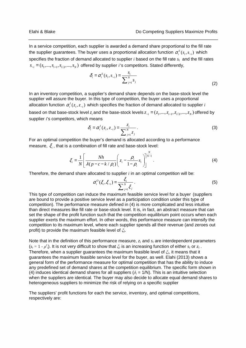
Loss Aversion Our results show that in competitions based on both service and inventory criteria, subjects playing the role of suppliers with identical costs will always reach stability with decisions significantly different that the Nash equilibrium points. However, when engaged in an optimal competition we do not see this pattern. Subjects’ average decisions, under optimal competition, are smaller than the corresponding Nash equilibrium, except for the less efficient supplier in the cases where the suppliers have heterogeneous costs. To gain insight into this behavior we first look at a supplier’s profit function with respect to the potential decisions that could made by competitors. This is because the share of demand allocated to a supplier depends on the decisions made by both the supplier and the supplier’s competitors. More specifically, we look at a supplier’s profit when their competitor chooses either the Nash equilibrium as their decision as well as chooses the average decision observed in our experiments. Figures 1 to 3 show these profit functions. The curves in these figures with the solid lines show a supplier’s expected profit for different decisions given that the competitor’s decision is at the Nash equilibrium value. The curves with a dashed line represent the supplier’s expected profit when a competitor’s decision is the average of the decisions we observed in our experiments. From these figures it can be seen that the rate of change in a supplier’s profit near its maximum point is much steeper for a service competition than either for an inventory or optimal competition. In other words, any deviation from the optimal decision is more costly for suppliers in a service competition in any other type. This observation might explain the gap between subjects’ decisions and the corresponding Nash equilibrium points in service competitions and why it is (almost always) smaller than the difference observed in either inventory or optimal competitions. The figures also show that in service competitions with heterogeneous suppliers with different production costs, subjects manage to (statistically) capture the Nash equilibrium. This is also the case for the more efficient supplier in service competitions where suppliers have different inventory holding costs. This can mean that, although an optimal competition can produce the best results for the buyer, it is difficult for subjects to capture the best decisions in an optimal competition due to the relatively flat profit functions around the decision which maximizes profit. The opposite is true for the service competition, in which the buyer receives a lower service level because subjects are able to reach the point where profits maximized. The figures also show that if a supplier’s competitor chooses the Nash equilibrium as their decision in an optimal competition (indicated by z2 = 77 in the rightmost chart of Figure 1), then any deviation the supplier makes other than matching the competitor’s decision will produce a negative profit. This means that subjects’ loss aversion can play an important role when engaged in this type of competition. When the suppliers have identical costs in an optimal competition, the only way suppliers can earn a positive profit is when both suppliers’ decisions are lower than the Nash equilibrium. Although this is not an equilibrium condition, any movement away from it can result in a negative profit, and this is exactly subjects’ behavior in our experiments. Instead of attempting to make decisions that would yield the maximum profits, they appear to have made decisions that would avoid receiving profits that were negative.

Elahi & Blake Do Competing Suppliers Maximize Profits
Figure 1: Profit functions for suppliers with identical cost structures
○ Nash Equilibrium (solid lines) □ Experimental Results (dashed lines)
Figure 2: Profit functions for suppliers with heterogeneous costs – different capacity costs (c)
○ Nash Equilibrium (solid lines) □ Experimental Results (dashed lines)
Figure 3: Profit functions for suppliers with heterogeneous costs - different holding costs (h)
○ Nash Equilibrium (solid lines) □ Experimental Results (dashed lines)
-20
0
20
40
60
0 20 40 60 80 100
z1
Service Competition
-20
0
20
40
60
0 20 40 60 80 100
z1
Inventory Competition
-20
0
20
40
60
0 20 40 60 80 100
z1
Optimal Competition
-15
0
15
30
45
60
0 20 40 60 80 100
z1 or z2
Service Competition
-15
0
15
30
45
60
0 20 40 60 80 100
z1 or z2
Inventory Competition
-15
0
15
30
45
60
0 20 40 60 80 100
z1 or z2
Optimal Competition
-15
0
15
30
45
60
0 20 40 60 80 100
z1 or z2
Service Competition
-15
0
15
30
45
60
0 20 40 60 80 100
z1 or z2
Inventory Competition
-20
0
20
40
60
80
0 20 40 60 80 100
z1 or z2
Optimal Competition
z2=19
(Nash)
z2=24
(Exper.)
z2=34
(Nash)
z2=54
(Exper.) z2=77 (Nash)
z2=68 (Exper.)
Profit 1
(Nash)
Profit 2
(Nash & Exper.)
(Exper.)
(Exper.)
Profit 1
(Nash)
Profit 2
(Nash) (Exper.)
Profit 1
(Nash)
(Exper.)
Profit 2
(Exper.)
Profit 1
(Nash)
Profit 2
(Nash & Exper.) (Exper.)
(Exper.)
Profit 1
(Nash)
Profit 2
(Nash) (Exper.)
Profit 1
(Nash)
(Exper.)
Profit 2
(Exper.)

Elahi & Blake Do Competing Suppliers Maximize Profits
CONCLUSIONS This research contributes by examining theoretical results applied to a model of outsourcing derived from prior work, and evaluates the theories in an experimental study. For this we conducted experiments with three types of competition between suppliers: service, inventory, and optimal. In each type of competition suppliers would compete for a single buyer’s demand allocated based on a measure of performance (competition criteria) defined and announced by the buyer prior to the start of competitions. Our experimental results show that the actual decisions competing suppliers make do not always match the decisions predicted by the Nash equilibrium. They show that the actual decisions are closest to the Nash equilibrium value in service competitions; in competitions based on the inventory and optimal criteria the differences are more pronounced. In most cases there are statistically significant differences between the actual decisions and theoretical predictions. The deviation of subjects’ decisions from the Nash equilibrium indicates that subjects do not always behave purely in a rational way as the Nash equilibrium assumes. A rational decision maker always aims to find the decision that will maximize expected profit. When decisions deviate from the Nash equilibrium value there might be behavioral influences that induce decisions that do not maximize profit. We therefore investigated reasons why subjects did not, or could not, maximize profits (i.e. reach the Nash equilibrium). In part, these deviations from theory can be accounted for by loss aversion behavior. Our supply chain model has important similarities to supply chains in the real world. Showing that the decisions that competing suppliers make do not always maximize profits, as theory predicts, is one important result from our study. Evaluating a behavioral influence as a potential explanation for this behavior is another important contribution. The findings from our study can be useful for buyers to determine the best means by which to award contracts, and for suppliers who need to understand potential influences that can lead decisions away from maximizing profits. Existing theory as it relates to the supply chain model we study has not yet been validated experimentally. Within the context of this model we compare actual decisions with theory by using experiments that involved different forms of competition and varying cost and industry structures. Further research could investigate additional scenarios and further generalize the findings from our study. In particular, for this study we could only conduct a limited number of experiments and therefore use a relatively small set of parameters for suppliers’ cost structures. We explored scenarios involving only two suppliers, and our model is based on specific assumptions, such how demand is generated. Relaxing these assumptions, analyzing the sensitivity of our results to the parameters we used, and expanding the range of scenarios could all be fruitful topics for further research. REFERENCES Anderson, L., & Stafford, S. (2003). An experimental analysis of rent seeking under varying competitive conditions, Public Choice, 115(1–2), 199–216. Anderson, L., & Freeborn, B. (2010). Varying the intensity of competition in a multiple prize rent seeking experiment, Public Choice, 143(1), 237–254.

Elahi & Blake Do Competing Suppliers Maximize Profits
Bell, C., Stidham, S., (1983). Individual versus social optimization in the allocation of customers to alternative servers. Management Science, 29(7), 831–839. Benjaafar, S., Elahi, E., Donohue, K., (2007). Outsourcing via Service Competition. Management Science, 53(2), 241–259. Cachon, G. P., Zhang, F., (2007). Obtaining Fast Service in a Queueing System via Performance-Based Allocation of Demand, Management Science, 53, 408-420. Chen, H. C., Friedman, J. W., Thisse, J. F., (1997). Boundedly Rational Nash Equilibrium: A Probabilistic Choice Approach, Games and Economic Behavior, 18, 32-54. Chen, H. C., Su, X., Zhao, X., (2012). Modeling Bounded Rationality in Capacity Allocation Games with the Quantal Response Equilibrium, Management Science. 58(10), 1952–1962. Davis, D., & Reilly, R. (1998). Do many cooks always spoil the stew? An experimental analysis of rent seeking and the role of a strategic buyer, Public Choice, 95, 89–115. Elahi, E., (2007). Outsourcing via Service Competition. PhD Dissertation, University of Minnesota. Ann Arbor: ProQuest/UMA. (ProQuest Document ID: 304837276). Elahi, E. (2013). Outsourcing through Competition: What is the Best Competition Parameter?, International Journal of Production Economic,s 144(1), 370-382. Gilbert, S., Weng, Z. K., (1998). Incentive Effects Favor Non-Competing Queues in a Service System: the Principal-Agent Perspective, Management Science, 44(12), 1662-1669. Ha, A.Y., Li, L., Ng, S. M., (2003). Price and Delivery Logistics Competition in a Supply Chain Management Science, 49, 1139-1153. Houser, D., Stratmann, T., (2012). Gordon Tullock and experimental economics, Public Choice, 152, 211–222. Jin, Y, Ryan, J. K., (2012). Price and Service Competition in an Outsourced Supply Chain: The Impact of Demand Allocation Policies, Production and Operations Management, 21(2), 331-344. Katok, E., Wu, D.Y., (2009). Contracting in Supply Chains: A Laboratory Investigation. Management Science,55(12), 1953-1968. Levine, D.M., Stephan, D.F., Krehbiel, T.C., Berenson, M.L., (2011). Statistics for managers, 6th edition, Prentice Hall. McKelvey R. D., Palfrey T.R., (1995). Quantal Response Equilibria for Normal Form Games, Games and Economic Behavior, 10(1), 6–38. Netessine, S., Rudi, N., Wang, Y., (2006). Inventory competition and incentives to back-order, IIE Transactions, 38, 883–902. Tullock, G. (1980). Efficient rent-seeking. In J. Buchanan, R. Tollison, & G. Tullock (Eds.), Toward a theory of the rent-seeking society, Texas A&M Press, 97-112.

Elahi & Blake Do Competing Suppliers Maximize Profits
Zhou, Y., Ren, Z. J., (2010). Service Outsourcing. In: Cochran et al. (Ed.), Wiley Encyclopedia of Operations Research and Management Science, Wiley. APPENDIX A This screen shot is from the software we developed for this research and is of the screen subjects used while experiments were being conducted. The results from each round are shown on the left of the screen as the competition progresses, and the calculation tool used to analyze pro-forma profits based on potential decisions by a supplier and a competitor is displayed on the right hand side of the screen: