Do Asset Fire Sales Exist? An Empirical Investigation of ...piazzesi/Reading/Pulvino 1998.pdf · Do Asset Fire Sales Exist? An Empirical Investigation of Commercial Aircraft Transactions

Do Asset Fire Sales Exist? An EmpiricalInvestigation of Commercial

Aircraft Transactions

TODD C. PULVINO*

ABSTRACT

This paper uses commercial aircraft transactions to determine whether capitalconstraints cause firms to liquidate assets at discounts to fundamental values.Results indicate that financially constrained airlines receive lower prices than theirunconstrained rivals when selling used narrow-body aircraft. Capital constrainedairlines are also more likely to sell used aircraft to industry outsiders, especiallyduring market downturns. Further evidence that capital constraints affect liqui-dation prices is provided by airlines’ asset acquisition activity. Unconstrained air-lines significantly increase buying activity when aircraft prices are depressed; thispattern is not observed for financially constrained airlines.

Eastern needs substantial liquidity to implementits business plan and expects that it will continueto sell assets to provide such liquidity.

—Texas Air, 1989 Annual Report

OPTIMAL CAPITAL STRUCTURE THEORIES suggest that firms choose debt levels suchthat tax and agency benefits of debt are balanced with expected costs offinancial distress. Although direct costs of financial distress ~e.g., legal andadministrative costs of bankruptcy! are well documented, comparatively littleevidence exists on indirect costs.1 This paper presents evidence on a specific

* Assistant Professor of Finance, Kellogg Graduate School of Management, NorthwesternUniversity. This research has benefited substantially from the comments of an anonymousreferee, Chris Avery, George Baker, Richard Caves, Tim Conley, Tony Davila, Robert Kennedy,Kentaro Koga, Josh Lerner, Tim Opler, Megan Partch, Andrei Shleifer, René Stulz, and seminarparticipants at the University of Chicago, Dartmouth University, Duke University, HarvardUniversity, the University of Illinois, M.I.T., the University of North Carolina, NorthwesternUniversity, the University of Oregon, the University of Rochester, the Wharton School, and theUniversity of Wisconsin. I would like to thank Howard Chickering and Steve O’Neil of R.V.I.Services, Mort Beyer of Mort Beyer Associates, Ken Raff of American Airlines, Carl Rings ofNorthwest Airlines, and Steven Gibbs of the FAA for useful discussions, and Chris Allen forassistance with data collection. Financial support from the Harvard Business School Division ofResearch is gratefully acknowledged.

1 For estimates of direct costs of bankruptcy, see Warner ~1977!, Altman ~1984!, and Weiss~1990!. Each of these studies finds that direct bankruptcy costs amount to less than 5 percentof firms’ prebankruptcy market values. Maksimovic and Phillips ~1996!, Chevalier ~1995!, Oplerand Titman ~1994!, Brown, James, and Ryngaert ~1992!, Kim and Maksimovic ~1990!, and Altman~1984!, examine indirect costs of financial distress.

THE JOURNAL OF FINANCE • VOL LIII, NO. 3 • JUNE 1998

939

indirect cost, namely, price discounts associated with distressed asset sales.Using a large sample of commercial aircraft transactions, I estimate themagnitude of the discount at which distressed airlines liquidate assets.

Empirical efforts to measure discounts at which assets are liquidated arecomplicated by the inability to measure fundamental values.2 As a result,previous studies have focused on stock price reactions to liquidation an-nouncements; they generally interpret positive reactions to mean that assetsare not being liquidated at discounts to fundamental values, but instead arebeing reallocated to higher-value users. However, these studies find conf lict-ing results ~e.g., see Brown, James, and Mooradian ~1994! and Lang, Poulsen,and Stulz ~1995!!.3 Lang et al. ~1995! argue that a possible cause of theconf lict is that announcements of decisions to sell assets convey informationnot only about the value of the asset sold, but also about the intended use ofproceeds and the financial health of the firm. They conclude that disentan-gling these effects may require analysis of a larger sample of less significantasset sales than has been used in previous empirical studies.

Unlike prior research, I estimate liquidation discounts by examining pricesat which assets are liquidated. I motivate this empirical work by applyingthe Shleifer and Vishny ~1992! industry-equilibrium model of asset liquida-tion to the commercial aircraft market. According to their model, discountsat which assets are sold will be particularly large in depressed industrieswhere assets are industry-specific. The reason is that competitors of dis-tressed firms may be facing financial constraints of their own and thereforewill be unable to pay fundamental values for assets. The result is that, dur-ing industry recessions, the market for industry-specific assets will be illiq-uid. Rather than selling to the highest-value user, distressed firms may beforced to sell to well-financed, low-value users.

Empirical results presented in this paper show that airlines’ financial con-ditions are key determinants of prices they receive for aircraft. Airlines withlow spare debt capacities ~defined to be airlines with above-industry-medianleverage ratios and below-industry-median current ratios! sell aircraft at a14 percent discount to the average market price. This discount exists whenthe airline industry is depressed but not when it is booming. An examinationof the effect of the quantity of sales provides some evidence that this isdriven in part by thinness in the market for used aircraft. Especially duringindustry recessions, an increase in the number of aircraft sold by an airlinein a given calendar-quarter results in a reduction in the price that the sellerreceives.

Examination of aircraft buyers provides additional evidence that finan-cially constrained airlines receive lower prices than unconstrained rivals.Because financial institutions ~e.g., banks and leasing companies! are lower-

2 I define “fundamental value” to be the net present value of cash f lows generated by an asset.3 Also see Hite, Owers, and Rogers ~1987!, Alexander, Benson, and Kampmeyer ~1984!, and

Jain ~1985!.

940 The Journal of Finance

value users of commercial aircraft than airlines, they tend to pay lower prices.This is the case particularly during industry recessions when competitionfor used aircraft is weak and the risk associated with finding a lessee for theaircraft is high. During market recessions, financial institutions pay a dis-count of 30 percent to the average market price. Furthermore, as sellers’financial constraints become more severe, the likelihood of selling to finan-cial institutions increases, but only during market recessions.

Finally, the pattern of airlines’ used aircraft purchases supports the hy-pothesis that financially constrained airlines liquidate aircraft at discountsto fundamental values. Airlines with high spare debt capacities tend to buymore used aircraft than airlines with low spare debt capacities, particularlywhen aircraft prices are depressed.

These results have important implications for firms’ capital structure de-cisions. They suggest benefits to limiting financial leverage; rather thanbeing forced to sell assets at discounts, maintaining spare debt capacity al-lows firms to be on the “buy-side” of industry fire sales. Results presented inthis paper also have implications for investment theories. They confirm thatinvestment abandonment is costly, and consistent with previously publishedempirical findings, they imply higher costs of capital stock adjustment thanstandard neoclassical theories of investment assume ~Hubbard ~1995! andCummins, Hassett, and Hubbard ~1994!!.

Finally, results presented in this paper have implications for the debateover bankruptcy law reform. Some authors argue that insolvent firms shouldbe forced into immediate cash liquidation via Chapter 7 of the U.S. bank-ruptcy code ~e.g., Baird ~1986!!, but opponents object to this solution on thegrounds that it may fail to maximize proceeds to liquidating firms’ claim-holders ~e.g., Aghion, Hart, and Moore ~1992!!. They argue that problemsassociated with raising capital and lack of competition for distressed firms’assets will cause liquidating firms to sell assets at discounts to fundamentalvalue. According to the Shleifer and Vishny ~1992! model, assets will be trans-ferred to well-financed industry outsiders who, because of the industry-specific nature of assets, are less productive users. Results presented in thispaper imply that immediate cash liquidation of distressed firms’ assets viaChapter 7 of the U.S. bankruptcy code could result in suboptimal outcomes;claimholders may get only a fraction of the value of their assets and assetsmay be distributed to financially unconstrained buyers rather than high-value users.

Section I presents a brief summary of the Shleifer and Vishny ~1992! modelas well as an application of their model to the used aircraft market. Testablehypotheses are also identified in this section. Section II describes the sampleof aircraft transactions used in the paper’s empirical analyses. Section IIIpresents the empirical methodology and results, and also discusses implica-tions of these results for the hypotheses presented in Section I. Section IVdiscusses an alternative explanation and Section V summarizes the mainresults and conclusions.

Do Asset Fire Sales Exist? 941

I. Theory

A. The Shleifer and Vishny Model

Shleifer and Vishny ~1992! consider the scenario where a firm responds tofinancial distress by selling assets. Whether the assets are sold to a buyerwithin the industry or to an outside buyer depends both on buyers’ funda-mental values and their abilities to pay. Differences in valuations betweeninside and outside buyers depend largely on characteristics of the assetsbeing sold. If assets are industry specific, an inside buyer is likely to placea higher value on the assets than an outsider. Oil refineries exemplify industry-specific assets; they generate large cash f lows when used to refine oil butsignificantly smaller cash f lows when deployed elsewhere. If assets are ge-neric, then inside buyers and outside buyers are likely to place similar val-ues on the assets. Computers exemplify generic assets; they can be usedproductively in any number of industries.

Even if the inside buyer is a more productive user, and therefore places ahigher value on the assets, the selling firm may sell to the industry outsider.This will be particularly true during industry recessions when factors thatforce the seller to liquidate also create financial constraints for potentialinside buyers. In this situation, the inside buyer is unable to offer funda-mental value for the selling firm’s assets. If the insider’s financial con-straints are much more severe than those of the outsider, the outsider willoutbid the insider and assets will be redeployed to a lower-value use.

B. Description of the Used Aircraft Market

There are many participants in the market for used commercial aircraft.In addition to airlines, aircraft are often purchased by governments, aircargo companies, and financial institutions. Some financial institutions areleasing companies whose primary business involves “placing” aircraft withlessees. However, banks and limited partnerships have also been active inbuying, leasing, and selling commercial aircraft.

The market for used commercial aircraft has historically been dominatedby privately negotiated transactions. Most major airlines have staff devotedto the acquisition and disposition of aircraft. Independent aircraft brokershave also been used to match buyers and sellers. Since the mid- to late1980s, firms dedicated to tracking commercial aircraft ~by serial number!have emerged, making it much easier for potential buyers to determine theowner of any given aircraft. These firms have also begun to publish “clas-sified advertisements” for commercial aircraft, thus reducing the need forbrokers. For example, Federal Express Aviation Services’ Availability Re-ports list aircraft available for sale or lease along with owners’ identities andphone numbers. However, asking price is rarely disclosed.

In the mid-1990s, auctions were organized to further improve liquidity inthe used aircraft market. One of the first such auctions was held in LasVegas, Nevada, in November 1994. Of 35 aircraft offered for sale, only nine


were sold. Subsequent auctions were even less successful. An auction in Se-attle, Washington, in September 1995 ended without a single sale—a sub-sequent auction scheduled for October 1995 was canceled because of lacklusterinterest at the Seattle auction. At least for the time being, the structure ofthe used commercial aircraft remains, as it has been for the past 20 years,dominated by privately negotiated transactions.

In a typical month, approximately 20 used commercial aircraft trade handsworldwide. For any given aircraft model, there are, on average, only one ortwo transactions per month. Thus, compared to financial markets, the mar-ket for used commercial aircraft is extremely “thin.” This makes it difficultfor buyers and sellers to establish “market values.” Because of difficulty inestablishing a benchmark market price, the relative bargaining powers ofbuyers and sellers are potentially important determinants of transaction price.Motivated sellers are more likely to agree to a low transaction price andmotivated buyers are more likely to agree to a high transaction price. Thispaper focuses on one particular source of motivation, namely, the financialcondition of the seller.

C. Application of Shleifer and Vishny to the Used Aircraft Market

In deciding whether to keep or sell an aircraft, distressed airlines comparethe net benefit from keeping the aircraft to the cash obtained by selling it. Thenet benefit from keeping an aircraft is comprised of the difference between thecash f low generated by the aircraft and the cost incurred in raising capital nec-essary to avoid default on existing loans. There are a number of potential sourcesof costs of raising capital. If the seller attempts to obtain capital from theexternal capital market, he must overcome information asymmetry.4 Costs ofdoing so will be particularly high when the seller is financially distressedbecause distress may signal managerial incompetence. Furthermore, inves-tors may not share management’s opinion about the value of assets in place.To entice investors to provide additional capital, securities may have to beoffered at a discount ~Myers and Majluf ~1984!!. In the extreme case, debtoverhang will prevent the seller from issuing new securities ~Myers ~1984!!.

Because proceeds from positive net-present-value ~NPV! projects can beused to pay existing creditors, the debt overhang that prevents the sellerfrom issuing new securities does not eliminate the possibility of resched-uling debt. Nevertheless, debt rescheduling may also be expensive. First,coordinating dispersed creditors may be costly ~Gertner and Scharfstein ~1991!,Asquith, Gertner, and Scharfstein ~1994!!. Second, creditors may worry thatdelaying debt payments will allow managers to pursue highly volatile neg-ative NPV projects ~Jensen and Meckling ~1976!, Myers ~1997!!. To preventthis, creditors incur increased monitoring costs, which are ultimately passedalong to the debtor.

4 For an example of costly investor communication, see Healy’s and Palepu’s ~1995! clinicalstudy of CUC International, Inc.


As the cost of raising capital increases, the net benefit ~i.e., cash f lowsgenerated from aircraft less the cost of raising capital! to the seller fromkeeping the aircraft decreases. Therefore, the price at which the seller isindifferent between keeping and selling the asset is decreasing in the seller’sdegree of financial distress ~or, equivalently, increasing in the seller’s sparedebt capacity! and decreasing in the dispersion of the seller’s creditors.

In order for an aircraft transaction to take place, it must be that buyersare both willing and able to pay a price that exceeds the seller’s reservationprice. The maximum price that buyers are willing and able to pay dependsboth on their valuations of the aircraft being sold and on their access tocapital. Other airlines ~industry insiders! are likely to be the most produc-tive users of used aircraft and are therefore likely to place the highest valueson these aircraft. However, if factors causing the seller’s distress are industry-wide, other airlines may not be in the financial position to acquire addi-tional aircraft even though doing so represents a positive NPV project. Theprice they will be able to pay equals the difference between the net presentvalue of cash f lows generated by the aircraft and the cost of raising capitalto finance the purchase. In an industry-wide recession, financial constraintsfaced by other airlines may be so severe that lower-value users ~industryoutsiders! are able to outbid airlines for their distressed competitors’ assets.

Financial institutions ~e.g., banks and aircraft leasing companies! tend tobe lower-value users of used aircraft. The reason is that, unlike airlines,financial institutions cannot immediately place aircraft in service and gen-erate revenue—they must first find a lessee. Although this is relatively easywhen demand for aircraft is high, it can be quite difficult and expensivewhen demand is low. Thus, net cash f lows generated by financial institu-tions tend to be lower than those generated by other airlines by an amountat least as large as the cost of “placing” the aircraft.5 Therefore, we wouldexpect to see, on average, lower transaction prices when the buyer is a fi-nancial institution. Because of this, sellers will prefer to sell to high-valueinsiders; desperate sellers will be more likely than patient sellers to sell tofinancial institutions. This effect should be particularly strong during mar-ket recessions, when competition from other airlines for the distressed sell-er’s assets is weak.

The foregoing discussion assumes that there is limited competition amongindustry buyers for distressed firms’ assets. This may be an unreasonableassumption in extremely liquid financial markets, but it is reasonable in the

5 When airlines have multiple years of negative earnings, profitable financial institutionsmay actually be higher value users of commercial aircraft. The reason is that the value of thedepreciation tax shield will be zero for an airline with negative earnings and positive for aprofitable financial institution. Depending on the magnitude of this tax shield, realized cashf lows may be greater for the financial institution. In this case, financial institutions would bewilling to pay more for used aircraft than would other airlines, especially during market re-cessions. However, this is not consistent with empirical evidence presented in a later section ofthis paper; financial institutions tend to pay lower prices than other airlines, particularly dur-ing depressions in the used aircraft market.


used aircraft market where transactions are less frequent and search coststhat sellers incur to find high-value buyers are relatively high. Evidencethat the used aircraft market is often illiquid is provided by the followingdisclaimer commonly included in aircraft appraisals:

The ‘Fair Market Value’ of the Aircraft . . . is the price which, in theopinion of Avmark @the appraiser#, could be negotiated in an arm’s lengthfree market transaction between a willing seller and a willing and ablebuyer, neither of whom is under undue pressure to complete the trans-action. In the event a distress sale is required, realization could be sig-nificantly less than the Fair Market Value.6

This implies that an opportunity exists for well-financed airlines. If aircraftsell at distressed prices during market recessions, we would expect to ob-serve increased buying activity by those insiders with relatively low costs ofaccessing capital.

D. Testable Hypotheses

Based on the above discussion, the following null and alternative hypoth-eses are obtained:

H01: Price is independent of the seller’s financial condition.HA1: Price is decreasing in the seller’s cost of raising capital.

~i! Price is increasing in the seller’s spare debt capacity.~ii! Price is decreasing in the number of seller’s creditors.

H02: Price is independent of the seller’s valuation of the aircraft.HA2: Price is positively related to the seller’s valuation of the aircraft.

H03: Price is independent of buyer identity (i.e., airline versus financial in-stitution).

HA3: Price is lower when the buyer is an industry outsider, especially duringindustry recessions.

H04: Buyer identity is independent of the seller’s financial condition.HA4: Financially constrained airlines are more likely to sell to financial in-

stitutions, particularly during market recessions.

H05: The number of used aircraft purchases per calendar-quarter is inde-pendent of the buyer’s spare debt capacity.

HA5: Spare debt capacity is positively related to the number of used aircraftpurchases, particularly during market recessions.

6 Source: People Express 14% Secured Equipment Certificate Prospectus, June 13, 1985,p. 11.


II. Data Description

Empirical analyses presented in this paper are based on used aircrafttransactions that occurred from 1978 to 1991. Examination of aircraft saleshas three advantages over the plant or division sales examined in previousstudies. First, aircraft of a given model are relatively homogeneous. Thismakes it easier to isolate effects of transacting parties’ characteristics ontransaction attributes ~e.g., price, timing of sale!. Second, the U.S. airlineindustry provides a sample of firms with widely varying capital structuresand profit levels. This variability allows inferences regarding effects of firms’financial conditions on asset liquidation decisions to be made. A final ad-vantage of using aircraft transactions is that, because of the global nature ofthe market for commercial aircraft, there are many buyers and sellers. Thisincreases liquidity and diminishes the importance of transacting parties’ char-acteristics. Results presented in this paper are likely to be amplified in in-dustries where used asset markets are less liquid.

Data used in this paper are based on Department of Transportation ~DOT!and Federal Aviation Administration ~FAA! filings assembled by Avmark Inc.,an aircraft appraisal and aviation consulting firm.7 Both the DOT and theFAA track histories of all commercial aircraft operating in the United States.They record the aircraft serial number, buyer identity, seller identity, priceat which the aircraft was traded, date of trade, and whether the transactioninvolved a straight sale or a sale0leaseback. Additionally, they provide tech-nical information including engine type, engine stage categorization, andaircraft age.8

Avmark assembled data on transactions from 1978 to 1993 for which pricewas disclosed. Prior to 1992, the Department of Transportation required pricedisclosure for all aircraft purchased or sold by U.S. corporations. Therefore,except for aircraft transactions associated with airline mergers or as part oflease agreement terminating conditions, the pre-1992 data set contains vir-tually all transactions that involved at least one U.S. party.9

After the DOT eliminated its price disclosure requirement, airlines andleasing companies generally stopped reporting transaction prices. Thus, post-

7 Avmark obtained most of the data from Department of Transportation Forms 41B-6 and41B-7.

8 Stage categorization refers to engine noise output. Stage 1 aircraft are the loudest; they arerestricted from operating in U.S. airspace. Stage 2 aircraft are quieter, but they too will berestricted from operating in U.S. airspace by the year 2000. All new aircraft, as well as someolder aircraft such as the DC-10, comply with Stage 3 requirements. Stage 2 aircraft can beretrofitted to comply with Stage 3 requirements. For example, upgrading a Boeing 727 aircraftfrom Stage 2 to Stage 3 costs $1.8 million to $2.6 million depending on the exact aircraft model~Source: Federal Express Aviation Services!.

9 Avmark claims that their database contains all transactions that occurred from 1978 to1991. To check completeness of the Avmark database, I assemble end-of-year f leet descrip-tions from airlines’ 10-Ks and annual reports. Changes in reported f leet sizes between yearsare compared to changes implied by transactions contained in Avmark’s database. Differencesare small, implying that the Avmark database is fairly comprehensive. Inconsistencies that aredetected generally involve military conversions or decisions to scrap older aircraft.


1991 transactions are included in the Avmark database only when priceswere voluntarily disclosed or reported in other public sources. To precludesample selection bias, transactions that occurred after 1991 are excludedfrom the analyses that follow.

Analyses presented in this paper focus on purchases and sales of usednarrow-body aircraft by U.S. airlines listed in Table I. Sales by other par-ties, primarily financial institutions, air cargo services, and foreign airlines,are used only to establish market prices. This eliminates the possibility thatresults are biased by uncontrolled cross-industry or cross-country effects.10

10 Much of the analysis that follows relates firms’ financial characteristics to their buyingand selling behaviors. Because financial institutions have capital structures that are very dif-ferent from airlines’ capital structures, including financial institutions in the analysis wouldmake results difficult to interpret.

Table I

Summary of Aircraft Purchase and Sale TransactionsTable entries indicate the total numbers of purchases and sales of used narrow-body aircraftover the 1978–1991 time period.

AirlineNumber of Used

Narrow-Body PurchasesNumber of Used

Narrow-Body Sales

Air Florida 11 15AIRCAL 0 3Alaska Airlines 17 9Aloha Airlines 0 3America West Airlines 16 8American Airlines 37 48Braniff Airlines 1 55Continental Airlines 28 15Delta Airlines 5 50Eastern Airlines 47 162Frontier Airlines 6 0Hawaiian Airlines 0 4Midway Airlines 43 6Muse Air 7 0New York Air 2 0Northwest Airlines 10 71Ozark Airlines 12 2Pacific Southwest 4 25Pan Am World Airways 7 33People Express Airlines 44 0Piedmont Airlines 28 5Republic Airlines 21 9Southwest Airlines 1 0Trans World Airlines 9 48United Airlines 38 82USAIR 36 26Western Airlines 6 25

Total 436 704


Data on U.S. airlines are obtained from a number of sources. Financialdata and f leet descriptions are obtained from COMPUSTAT, company 10Ksand 10Qs, and the 1978 through 1991 volumes of Moody’s TransportationManual. When available, quarterly data are used; otherwise annual dataare collected. Airlines’ operating statistics are obtained from Air Carrier Traf-fic Statistics ~1978–1984 and 1985–1991!. Specific dates of airline mergersand bankruptcies are obtained from the Capital Changes Reporter, pub-lished by Commerce Clearing House, Inc.

III. Empirical Methodology and Results

To distinguish between the null and alternative hypotheses listed in Sec-tion I, in this section I examine ~A! determinants of transaction price, ~B!effect of the seller’s spare debt capacity on buyer identity, and ~C! factorsaffecting airlines’ purchase decisions. Empirical methodologies, results, andtheoretical implications are presented.

A. Effects of Seller’s Financial Characteristics and Buyer’s Identity on Price

A.1. Methodology

According to the null hypothesis, buyers’ and sellers’ financial character-istics should not affect aircraft prices. Conversely, the alternative hypothesispredicts that price will be increasing in the seller’s spare debt capacity, de-creasing in the number of the seller’s creditors, and increasing in the seller’svaluation of the aircraft. The alternative hypothesis also predicts that ob-served prices will be lower when the buyer is a financial institution. Onepossible way to test these hypotheses would be to assemble a sample oftransaction pairs with transactions matched by aircraft model, aircraft age,and the calendar-quarter in which they occurred. The only difference be-tween transactions in a pair would be the financial condition of the seller orthe identity of the buyer. Unfortunately, there are not enough transactionsto employ this methodology—generating an adequate number of pairs wouldrequire excessive relaxation of the requirements that transactions within apair be of the same model and age, and occur in the same calendar-quarter.Therefore, to determine the effects of sellers’ financial characteristics andbuyers’ identities on transaction prices, I employ hedonic regression meth-odology.11 Use of the hedonic procedure eliminates the need to match trans-actions. It also avoids estimation of time-varying supply and demand equations;calendar-quarter dummies included as independent variables account for tem-poral changes in equilibrium price.

11 For an overview of hedonic regression models, see Berndt ~1991!, Chapter 4. The approachused in this paper is similar to that used by Lerner ~1994! in his analysis of rigid disk drivepricing.


The hedonic regression approach requires a two-step procedure. First,hedonic prices for narrow-body aircraft are calculated using the followingequation:

log~PRICE! 5 bo 1 (i51

I

biMODELi 1 (j51

J

bjQTRj

1 (k51

K

bkSTAGEk 1 bAGE log~1 1 AGE! 1 e, ~1!

where PRICE 5 transaction price,12 QTR 5 dummy variables representingcalendar-quarters, MODEL 5 dummy variables representing aircraft mod-els,13 STAGE 5 dummy variables representing engine stage categories, andAGE 5 aircraft age at time of transaction. Independent variables included inthe hedonic regression are identified based on discussions with industry par-ticipants concerning important determinants of commercial aircraft prices.Logarithm of the transaction price ~as opposed to simply price! is used as thedependent variable to impose a ~price! nonnegativity constraint on the model.

Only narrow-body models for which at least 15 transactions occurred be-tween 1978 and 1991 are used to estimate equation ~1!. This results in atotal of 13 narrow-body models.14 Although including other aircraft modelswould increase the sample size, it may also diminish the accuracy of thehedonic regression coefficients. Limiting aircraft models to those with morethan 15 transactions mitigates this possibility. To avoid singularity, dummyvariables representing the third quarter of 1991, Stage 3 aircraft, and Air-bus 300B4-200 models are omitted when estimating equation ~1!. Therefore,eb0 represents the estimated price in third quarter 1991 of an Airbus 300B4-200 that is zero years old.15 Results from estimation of equation ~1! arepresented in Appendix A.

To the extent that MODEL, STAGE, and AGE control for quality differ-ences, residuals from this estimation are independent of aircraft quality andoverall market conditions. Therefore, in the second step of the hedonic pric-ing procedure, residuals ~RES! are regressed on transaction-specific explan-atory variables.

An alternative to the two-step procedure described here would be to per-form only one estimation; price could be regressed on aircraft variables

12 All prices are inf lation-adjusted using the producer price index.13 Equation ~1! is also estimated after including additional dummy variables to represent

engine type. Including these dummies substantially reduces the number of degrees of freedombut only increases the adjusted R2 from 0.762 to 0.766. Therefore, engine variant dummies areomitted from the analysis.

14 For a list of narrow-body models included in this analysis, see model dummy variables inthe hedonic regression results presented in Table A.I.

15 Such an aircraft does not exist; Airbus stopped building 300B4-200s in the late 1980s. Butif it did exist, its price would be eb0. ~This example is given only to demonstrate coefficientinterpretations.!


~MODEL, STAGE, AGE!, time dummies, and transaction-specific explana-tory variables. The disadvantage of this single-step procedure is that onlydata points for which second-stage independent variables exist ~i.e., whenthe seller is a U.S. airline! can be included in the regression. The two-stepprocedure on the other hand uses all transactions to estimate time, model,age, and stage coefficients. This results in more accurate hedonic prices.16

A.2. Variables

Explanatory variables include proxies for sellers’ spare debt capacities andfuture prospects. Also included are the number of aircraft sold in the calen-dar quarter and dummy variables specifying buyer identity ~i.e., whetherthe buyer is an industry insider or outsider!.

As proxies for spare debt capacity, I construct variables based on airlines’leverage and current ratios relative to industry medians in each calendar-quarter.17 Leverage ratio is defined as book value of debt plus capitalizedlease obligations divided by the sum of book value of debt, capitalized leaseobligations, and book value of equity. Capitalized lease obligations are in-cluded in the leverage ratio calculation to account for the fact that, underSection 1110 of U.S. bankruptcy code, capitalized leased obligations are es-sentially treated as “super-senior” debt. Under Section 1110, aircraft lessorsare relieved from automatic stay provisions that affect most creditors duringChapter 11 proceedings; lessors have the right to seize “collateral” 60 daysafter the lessee violates the lease contract. Book value of equity is usedinstead of market value of equity to minimize the possibility of leveragemeasuring economic rather than financial distress.

Because firms classified as having high leverage ratios are likely to befacing debt overhang, new investors will be reluctant to provide cash forpositive NPV projects. However, the mere existence of debt overhang shouldnot prevent firms from undertaking positive NPV projects. An airline withsevere debt overhang but a large cash balance will be able to finance invest-ment projects without accessing the external capital market. To control forthis possibility, I calculate current ratio, defined as current assets divided bycurrent liabilities. Firms with high current ratios are unlikely to be facingliquidity crises or capital constraints, regardless of leverage ratio. Only firms

16 Unreported estimations using the single-step procedure yield results similar to those ob-tained using the two-step approach.

17 A potential problem with this procedure is that by characterizing firms relative to theindustry median, I may be classifying firms as having low spare debt capacities even thoughthey ~and every other firm in the industry! have high spare debt capacities. However, this is notlikely to be a problem in the U.S. airline industry. Since the Airline Deregulation Act of 1978,there has been a continuous and abundant supply of highly leveraged and distressed airlines.Between January 1978 and December 1992, cumulative net income for U.S. airlines included inthe COMPUSTAT database was negative $3.06 billion in 1993 dollars. If anything, the approachfollowed in this analysis classifies low-spare-debt-capacity firms as having high spare debtcapacities.


with both high leverage ratios and low current ratios are likely to be finan-cially constrained. Based on the discussion presented in Section I, it is thesefirms that are most likely to sell assets at discounts to fundamental values.

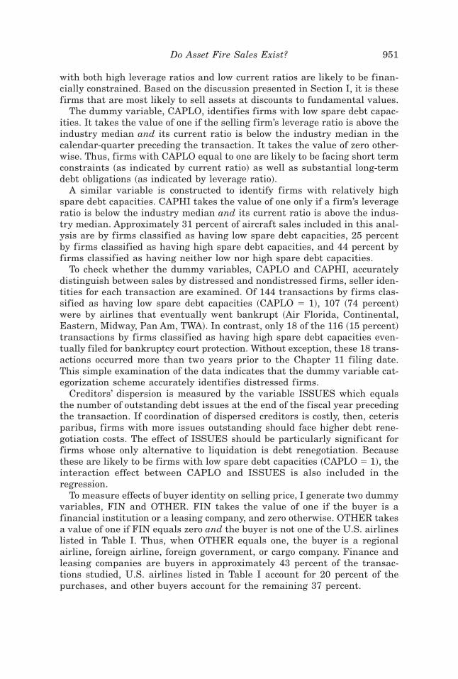
The dummy variable, CAPLO, identifies firms with low spare debt capac-ities. It takes the value of one if the selling firm’s leverage ratio is above theindustry median and its current ratio is below the industry median in thecalendar-quarter preceding the transaction. It takes the value of zero other-wise. Thus, firms with CAPLO equal to one are likely to be facing short termconstraints ~as indicated by current ratio! as well as substantial long-termdebt obligations ~as indicated by leverage ratio!.

A similar variable is constructed to identify firms with relatively highspare debt capacities. CAPHI takes the value of one only if a firm’s leverageratio is below the industry median and its current ratio is above the indus-try median. Approximately 31 percent of aircraft sales included in this anal-ysis are by firms classified as having low spare debt capacities, 25 percentby firms classified as having high spare debt capacities, and 44 percent byfirms classified as having neither low nor high spare debt capacities.

To check whether the dummy variables, CAPLO and CAPHI, accuratelydistinguish between sales by distressed and nondistressed firms, seller iden-tities for each transaction are examined. Of 144 transactions by firms clas-sified as having low spare debt capacities ~CAPLO 5 1!, 107 ~74 percent!were by airlines that eventually went bankrupt ~Air Florida, Continental,Eastern, Midway, Pan Am, TWA!. In contrast, only 18 of the 116 ~15 percent!transactions by firms classified as having high spare debt capacities even-tually filed for bankruptcy court protection. Without exception, these 18 trans-actions occurred more than two years prior to the Chapter 11 filing date.This simple examination of the data indicates that the dummy variable cat-egorization scheme accurately identifies distressed firms.

Creditors’ dispersion is measured by the variable ISSUES which equalsthe number of outstanding debt issues at the end of the fiscal year precedingthe transaction. If coordination of dispersed creditors is costly, then, ceterisparibus, firms with more issues outstanding should face higher debt rene-gotiation costs. The effect of ISSUES should be particularly significant forfirms whose only alternative to liquidation is debt renegotiation. Becausethese are likely to be firms with low spare debt capacities ~CAPLO 5 1!, theinteraction effect between CAPLO and ISSUES is also included in theregression.

To measure effects of buyer identity on selling price, I generate two dummyvariables, FIN and OTHER. FIN takes the value of one if the buyer is afinancial institution or a leasing company, and zero otherwise. OTHER takesa value of one if FIN equals zero and the buyer is not one of the U.S. airlineslisted in Table I. Thus, when OTHER equals one, the buyer is a regionalairline, foreign airline, foreign government, or cargo company. Finance andleasing companies are buyers in approximately 43 percent of the transac-tions studied, U.S. airlines listed in Table I account for 20 percent of thepurchases, and other buyers account for the remaining 37 percent.


In order to separate the effects of financial distress from effects of eco-nomic distress, three variables that measure firm prospects are included inthe regression. The first variable is an estimate of Q, equal to the sum ofbook value of debt and market value of equity divided by the sum of bookvalue of debt and book value of equity. As has been noted in the investment0cash f low literature, this measure of Q is f lawed in that it measures averagerather than marginal Q. Many authors posit that empirical findings of pos-itive relationships between investment and cash f low are simply a manifes-tation of average Q’s inability to measure firm prospects; that is, cash f lowmeasures firm prospects that are not correlated with average Q ~Fazzari,Hubbard, and Petersen ~1988!, Kaplan and Zingales ~1997!!. Therefore, Iinclude two measures for firms’ abilities to generate future cashf lows. REVequals load factor ~revenue-passenger-miles divided by available-seat-miles!times revenue per revenue-passenger-mile. This variable provides a mea-sure of airlines’ abilities to fill their planes with high-revenue passengers.The second proxy for selling firms’ abilities to generate cashf lows is COST,which equals cost-of-goods-sold divided by available-seat-miles. This pro-vides a measure of airlines’ cost efficiencies and may, for a given level ofREV, provide a more accurate proxy for “marginal” prospects.

To determine whether market thinness contributes to asset sale discounts,the variable NSALE is computed. NSALE equals the number of narrow-bodyaircraft that the selling airline sold in the calendar quarter of the transac-tion. If market liquidity is important, we should observe a negative relation-ship between number of narrow-body sales in the calendar-quarter andtransaction price.

Finally, I construct a price index variable, INDEX, which measuresinf lation-adjusted prices of narrow-body aircraft for each calendar-quarter,net of model type, and aircraft quality differences. INDEX is generatedfrom coefficients of calendar-quarter dummies used in the hedonic regres-sion ~equation ~1!!. By holding quality constant ~as measured by AGE, STAGE,and MODEL! and arbitrarily setting INDEX equal to 1.0 for the third quarterof 1991, the price index for quarter j can be obtained by calculating ebj wherebj is the coefficient of the quarter j dummy variable. Because the sample usedin this study covers 56 calendar-quarters, INDEX takes on 1 of 56 different val-ues in each calendar-quarter. Low values of INDEX indicate that the used air-craft market is depressed, high values indicate that it is booming.

All airlines that sold at least one of the 13 aircraft types used to estimateequation ~1!, and for which financial data are available, are included in thesecond stage of the hedonic procedure. Exceptions are liquidating trusts,Chapter 7 liquidations, and most Chapter 11 sales.18 Although these trans-actions are particularly pertinent to hypotheses being tested in this paper,they are only used if financial data for the calendar-quarter before the trans-action is available. Over the 1978–1991 time-period, only Braniff and East-

18 The effect of bankruptcy court protection on asset sale discounts is studied explicitly inPulvino ~1996!.


ern had significant numbers of narrow-body sales for which reliable financialdata are unavailable. From 1984 to 1990, Braniff Airlines and Braniff Liq-uidating Trust omissions consisted of 36 transactions at an average discountof 9.0 percent ~significantly different from zero at the 0.1 percent level!.There are 79 Eastern Airlines sales for which accurate financial data areunavailable. These aircraft were sold at an average discount of 5.2 percent,significantly different from zero at the 5 percent level. None of Pan Am’snarrow-body sales are omitted.

A.3. Results

Table II summarizes both the residual from estimation of equation ~1! andthe independent variables used in the cross-sectional analysis of residuals.Summaries are provided for the whole sample and also for subsamples seg-mented by selling firms’ spare debt capacities. Table II indicates that priceresidual is strongly correlated with spare debt capacity. Firms classified ashaving low spare debt capacities sell aircraft at a 14 percent discount tohedonic price. Discounts for firms classified as having either medium orhigh spare debt capacities are indistinguishable from zero. The difference indiscounts between these two groups and the low spare debt capacity group issignificant at the 5 percent level.

Table II also shows that airlines classified as having low spare debtcapacities have more debt issues outstanding, have lower levels of operat-ing income0sales, are smaller ~as measured by book value of assets!, andtend to sell younger airplanes than firms classified as having mediumspare debt capacities. These differences are all significant at or beyond the5 percent level. The difference in number of outstanding issues resultsfrom correlation of leverage ratio with both number of issues outstandingand spare debt capacity. Firms with higher leverage ratios are likely tohave more debt issues and, by definition, lower spare debt capacities. Sim-ilarly, differences in operating income0sales are likely driven by correlationbetween current ratio and both spare debt capacity and past operatingincome0sales.

Unlike financial variables, differences in firm size and aircraft age arenot caused by the construction of variables. The result that low spare debtcapacity firms sell “younger” airplanes is consistent with the alternativehypothesis. That is, sales by financially constrained firms may be driven bythe need to raise cash. Even though newer aircraft cost less to operate thanolder aircraft, ceteris paribus, more cash is generated from the sale of a newaircraft than an old aircraft.

Neither operating statistics ~load factor 3 revenue per revenue passengermile and cost of goods sold divided by available seat mile! nor Q vary sys-tematically with sellers’ financial conditions. However, the percentage of salesto financial institutions is greater for firms with low spare debt capacity.Financial institutions were buyers in 54 percent of the sales by low sparedebt capacity sellers compared to 29 percent for high spare debt capacity


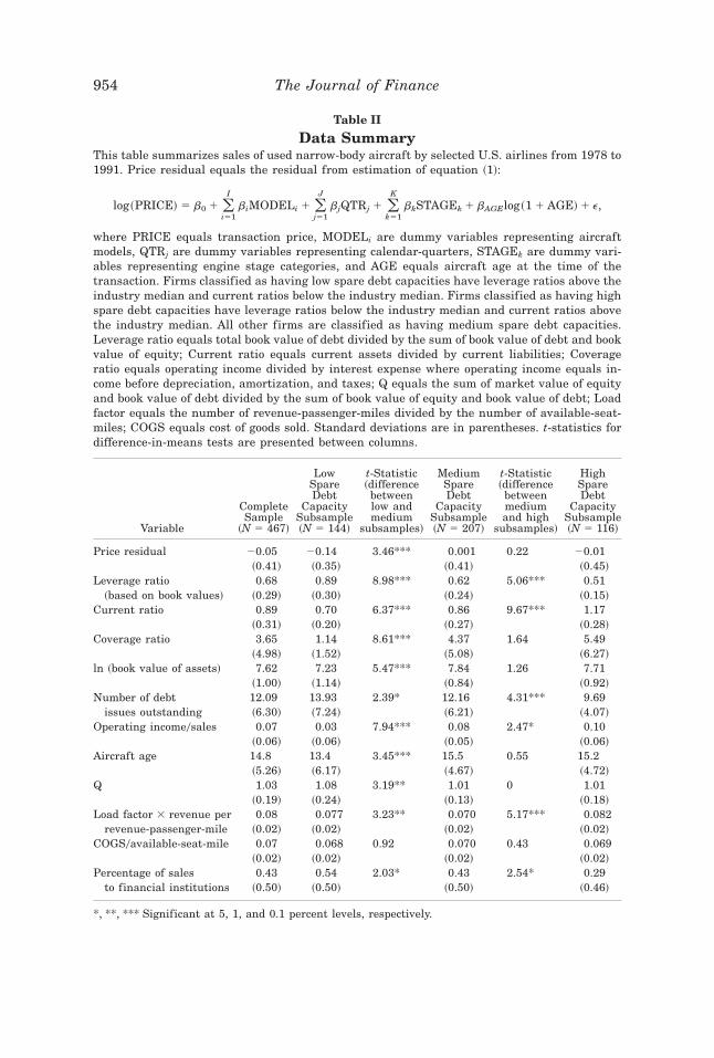
Table II

Data SummaryThis table summarizes sales of used narrow-body aircraft by selected U.S. airlines from 1978 to1991. Price residual equals the residual from estimation of equation ~1!:

log~PRICE! 5 b0 1 (i51

I

biMODELi 1 (j51

J

bjQTRj 1 (k51

K

bkSTAGEk 1 bAGElog~1 1 AGE! 1 e,

where PRICE equals transaction price, MODELi are dummy variables representing aircraftmodels, QTRj are dummy variables representing calendar-quarters, STAGEk are dummy vari-ables representing engine stage categories, and AGE equals aircraft age at the time of thetransaction. Firms classified as having low spare debt capacities have leverage ratios above theindustry median and current ratios below the industry median. Firms classified as having highspare debt capacities have leverage ratios below the industry median and current ratios abovethe industry median. All other firms are classified as having medium spare debt capacities.Leverage ratio equals total book value of debt divided by the sum of book value of debt and bookvalue of equity; Current ratio equals current assets divided by current liabilities; Coverageratio equals operating income divided by interest expense where operating income equals in-come before depreciation, amortization, and taxes; Q equals the sum of market value of equityand book value of debt divided by the sum of book value of equity and book value of debt; Loadfactor equals the number of revenue-passenger-miles divided by the number of available-seat-miles; COGS equals cost of goods sold. Standard deviations are in parentheses. t-statistics fordifference-in-means tests are presented between columns.

Variable

CompleteSample

~N 5 467!

LowSpareDebt

CapacitySubsample~N 5 144!

t-Statistic~differencebetweenlow andmedium

subsamples!

MediumSpareDebt


t-Statistic~differencebetweenmediumand high

subsamples!

HighSpareDebt


Price residual 20.05 20.14 3.46*** 0.001 0.22 20.01~0.41! ~0.35! ~0.41! ~0.45!

Leverage ratio 0.68 0.89 8.98*** 0.62 5.06*** 0.51~based on book values! ~0.29! ~0.30! ~0.24! ~0.15!

Current ratio 0.89 0.70 6.37*** 0.86 9.67*** 1.17~0.31! ~0.20! ~0.27! ~0.28!

Coverage ratio 3.65 1.14 8.61*** 4.37 1.64 5.49~4.98! ~1.52! ~5.08! ~6.27!

ln ~book value of assets! 7.62 7.23 5.47*** 7.84 1.26 7.71~1.00! ~1.14! ~0.84! ~0.92!

Number of debt 12.09 13.93 2.39* 12.16 4.31*** 9.69issues outstanding ~6.30! ~7.24! ~6.21! ~4.07!

Operating income0sales 0.07 0.03 7.94*** 0.08 2.47* 0.10~0.06! ~0.06! ~0.05! ~0.06!

Aircraft age 14.8 13.4 3.45*** 15.5 0.55 15.2~5.26! ~6.17! ~4.67! ~4.72!

Q 1.03 1.08 3.19** 1.01 0 1.01~0.19! ~0.24! ~0.13! ~0.18!

Load factor 3 revenue per 0.08 0.077 3.23** 0.070 5.17*** 0.082revenue-passenger-mile ~0.02! ~0.02! ~0.02! ~0.02!

COGS0available-seat-mile 0.07 0.068 0.92 0.070 0.43 0.069~0.02! ~0.02! ~0.02! ~0.02!

Percentage of sales 0.43 0.54 2.03* 0.43 2.54* 0.29to financial institutions ~0.50! ~0.50! ~0.50! ~0.46!

*, **, *** Significant at 5, 1, and 0.1 percent levels, respectively.


sellers. The difference between these percentages is significant at the 0.1 per-cent level.

RES 5 b0 1 b1CAPLO 1 b2CAPHI 1 b3ISSUE 1 b4~CAPLO 3 ISSUE!

1 b5FIN 1 b6OTHER 1 b7 Q 1 b8 REV 1 b9COST 1 b10NSALE 1 e.

~2!

Equation ~2! is used to assess effects of sellers’ spare debt capacities andfirm prospects on price residuals from the hedonic regression ~RES!. Thetypical assumption used to make statistical inferences based on regressionslike that specified in equation ~2! is that error terms are independently andidentically distributed. In this sample of used aircraft transactions, the in-dependence assumption may be problematic. Prices obtained for differentaircraft sold by the same airline in the same calendar quarter are likely tobe correlated. Furthermore, for an airline executing a f leet liquidation overtime, serial correlation in error terms is likely. Although ignoring this prob-lem would not bias coefficient estimates, it would cause errors in estimatesof standard errors. Therefore, in addition to presenting OLS standard er-rors, I present “pseudo-Newey–West” standard errors developed by Conley~1996!. These standard errors account for correlation between observationsby weighting the coefficient covariance matrix according to similarities be-tween transactions. For example, in a simple time-series setting, correlationbetween two observations is assumed to be greatest when the observationsare close in time. Newey–West covariance matrix weighting factors are closeto one for transactions that occur close in time and decrease to zero fortransactions that are distant in time. In the cross-section0time-series settingof this paper, transactions that have the same seller, buyer, date, and air-craft model are assumed to be close in terms of “economic distance.” Thesetransactions are assigned a covariance weighting factor of one. Observationsthat are separated by greater economic distances are assigned lower weight-ing factors. Detailed descriptions of weighting factors and standard errorcalculations are included in Appendix B. Here I will simply point out thatassumptions used to calculate standard errors are intentionally conservative—true standard errors are likely to lie somewhere between OLS standard er-rors and Conley ~1996! standard errors. For this reason, both are presentedin subsequent tables.

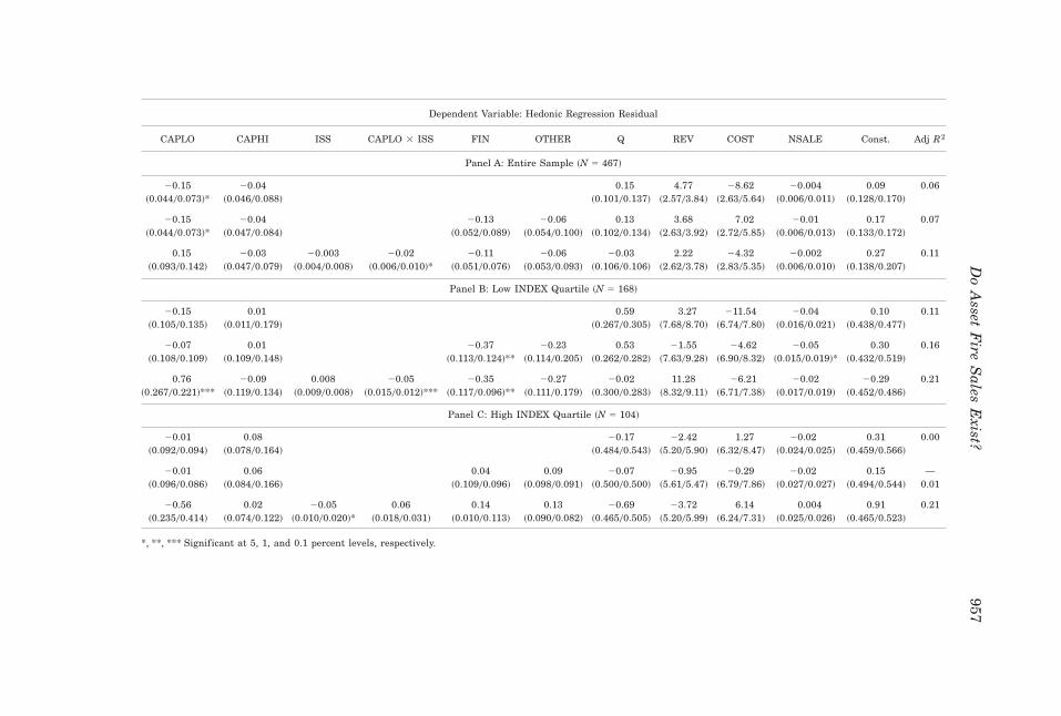
Results from estimating equation ~2! are presented in Table III. After con-trolling for firm prospects, firms classified as having low spare debt capac-ities ~CAPLO 5 1! sell aircraft at 13 percent discounts compared to firmsclassified as having neither low nor high spare debt capacities.19 This effect

19 Because the dependent variable, RES, equals the logarithm of the ratio of price to hedonicprice, discounts are calculated by taking the absolute value of one minus the exponent of thecoefficient. For example, the discount associated with having low spare debt capacity equals61 2 exp~b1!6.


Table III

OLS Regressions of the Determinants of Sale PriceThis table presents OLS regressions relating narrow-body transaction prices to selling airlines’ financial characteristics for 467 aircraft trans-actions. The dependent variable is the residual from the hedonic regression ~equation ~1!!:


I

biMODELi 1 (j51

J

bjQTRj 1 (k51

K

bkSTAGEk 1 bAGE log~1 1 AGE! 1 e,

where PRICE equals transaction price, MODELi are dummy variables representing aircraft models, QTRj are dummy variables representingcalendar-quarters, STAGEk are dummy variables representing engine stage categories, and AGE equals aircraft age at the time of the transac-tion. Panel A presents results using the entire sample, Panel B presents results using the subsample of transactions that occurred when theINDEX of used aircraft prices was in the lowest quartile, and Panel C presents results using the subsample of transactions that occurred whenthe INDEX of used aircraft prices was in the highest quartile. INDEX is calculated by exponentiating calendar-quarter dummy coefficients;CAPLO is a dummy variable equal to 1 if the selling airline’s leverage ratio was above the industry median and its current ratio was below theindustry median in the calendar-quarter preceding the transaction; CAPHI is a dummy variable equal to 1 if the selling airline’s leverage ratiowas below the industry median and its current ratio was above the industry median in the preceding quarter; ISS equals the number of debtissues outstanding in the calendar-quarter preceding the transaction; FIN is a dummy variable equal to 1 if the buyer is a financial or leasingcompany; OTHER is a dummy variable equal to 1 if the buyer is not a financial institution, leasing company, or large U.S. airline; Q equalsmarket value of equity plus book value of debt divided by book value of equity plus book value of debt; REV equals load factor ~equal torevenue-passenger-miles divided by available-seat-miles! times revenue per revenue-passenger-mile; COST equals cost-of-goods-sold divided byavailable-seat-miles; NSALE equals the number of narrow-body sales by the selling airline in the calendar-quarter of the transaction. Results arerelative to transactions where the seller has medium spare debt capacity and the buyer is a major U.S. airline. Both OLS and Conley ~1996!standard errors are presented in parentheses ~OLS standard errors are first!. The Conley ~1996! procedure corrects for correlation of observationsbased on proximity in economic distance.

956T

he

Jou

rnal

ofF

inan

ce

Dependent Variable: Hedonic Regression Residual

CAPLO CAPHI ISS CAPLO 3 ISS FIN OTHER Q REV COST NSALE Const. Adj R2

Panel A: Entire Sample ~N 5 467!

20.15 20.04 0.15 4.77 28.62 20.004 0.09 0.06~0.04400.073!* ~0.04600.088! ~0.10100.137! ~2.5703.84! ~2.6305.64! ~0.00600.011! ~0.12800.170!

20.15 20.04 20.13 20.06 0.13 3.68 7.02 20.01 0.17 0.07~0.04400.073!* ~0.04700.084! ~0.05200.089! ~0.05400.100! ~0.10200.134! ~2.6303.92! ~2.7205.85! ~0.00600.013! ~0.13300.172!

0.15 20.03 20.003 20.02 20.11 20.06 20.03 2.22 24.32 20.002 0.27 0.11~0.09300.142! ~0.04700.079! ~0.00400.008! ~0.00600.010!* ~0.05100.076! ~0.05300.093! ~0.10600.106! ~2.6203.78! ~2.8305.35! ~0.00600.010! ~0.13800.207!

Panel B: Low INDEX Quartile ~N 5 168!

20.15 0.01 0.59 3.27 211.54 20.04 0.10 0.11~0.10500.135! ~0.01100.179! ~0.26700.305! ~7.6808.70! ~6.7407.80! ~0.01600.021! ~0.43800.477!

20.07 0.01 20.37 20.23 0.53 21.55 24.62 20.05 0.30 0.16~0.10800.109! ~0.10900.148! ~0.11300.124!** ~0.11400.205! ~0.26200.282! ~7.6309.28! ~6.9008.32! ~0.01500.019!* ~0.43200.519!

0.76 20.09 0.008 20.05 20.35 20.27 20.02 11.28 26.21 20.02 20.29 0.21~0.26700.221!*** ~0.11900.134! ~0.00900.008! ~0.01500.012!*** ~0.11700.096!** ~0.11100.179! ~0.30000.283! ~8.3209.11! ~6.7107.38! ~0.01700.019! ~0.45200.486!

Panel C: High INDEX Quartile ~N 5 104!

20.01 0.08 20.17 22.42 1.27 20.02 0.31 0.00~0.09200.094! ~0.07800.164! ~0.48400.543! ~5.2005.90! ~6.3208.47! ~0.02400.025! ~0.45900.566!

20.01 0.06 0.04 0.09 20.07 20.95 20.29 20.02 0.15 —~0.09600.086! ~0.08400.166! ~0.10900.096! ~0.09800.091! ~0.50000.500! ~5.6105.47! ~6.7907.86! ~0.02700.027! ~0.49400.544! 0.01

20.56 0.02 20.05 0.06 0.14 0.13 20.69 23.72 6.14 0.004 0.91 0.21~0.23500.414! ~0.07400.122! ~0.01000.020!* ~0.01800.031! ~0.01000.113! ~0.09000.082! ~0.46500.505! ~5.2005.99! ~6.2407.31! ~0.02500.026! ~0.46500.523!


Do

Asset

Fire

Sales

Exist?

957

is significant at the 5 percent level when Conley ~1996! standard errors areused and even higher when OLS standard errors are used. The discount issimilar in magnitude to those suggested by Shleifer and Vishny ~1992! forhurried asset sales.20 Comparable results are obtained when the sample islimited to industry recessions ~Panel B!. However, reducing the sample sizeincreases the standard error and reduces statistical significance. Further-more, when buyer identity is included in the regression, the CAPLO coeffi-cient is reduced. As discussed below, this is probably caused by the propensityof financially distressed firms to sell to financial institutions during marketdownturns. Thus, it is difficult to disentangle the effect of capital con-straints on price from the effect of buyer identity on price. Discounts asso-ciated with financial distress are substantially reduced when the used aircraftmarket is booming ~Panel C!.

As an alternative to using the dichotomous variables CAPLO and CAPHIto classify firms’ levels of financial distress, continuous variables are alsoconsidered. Coverage ratio, equal to operating income divided by interestexpense, is a commonly suggested proxy for financial distress. However, thereare two problems with using coverage ratio. First, especially during marketrecessions, operating incomes are often negative. Assessing relative degreesof financial distress for firms with negative coverage ratios is difficult. Forexample, very distressed firms ~those with high interest expense and mod-estly negative operating income! have coverage ratios similar to those ofmoderately distressed firms ~those with low interest expense and slightlynegative operating income!. This is particularly problematic during severemarket recessions when even the median industry coverage ratio is nega-tive. The second problem with using coverage ratio to proxy for financialdistress is that, because operating income is in the numerator, coverage ra-tio may also proxy for economic distress. Nevertheless, using coverage ratioyields results similar to those obtained using the previously described di-chotomous variables. Aircraft sold by airlines with low coverage ratios aresold at a 15 percent discount; those sold by airlines with medium coverageratios are sold at a 4 percent discount, and those sold by airlines with highcoverage ratios are sold at a 5 percent premium. Differences in these dis-counts are significant at the 5 percent level.21

Interaction effects shown in Table III indicate that, for firms classified ashaving low spare debt capacities, the number of debt issues outstanding isnegatively correlated with transaction price. Summing the ISSUES and in-teraction term coefficients in the third specification of Panel A implies thata one standard deviation increase in the number of debt issues outstandingreduces price by 15 percent. This effect is more pronounced when the used

20 For example, Shleifer and Vishny ~1992! cite real estate appraisers’ estimates that rapidreal estate sales lead to price discounts of 15 to 25 percent relative to orderly sales ~p. 1358!.

21 Low-coverage ratio transactions correspond to the 100 transactions with the lowest cov-erage ratios. High-coverage ratio transactions correspond to the 100 transactions with the high-est coverage ratios.


aircraft market is depressed ~Panel B! and nonexistent when the market isbooming.

According to the null hypothesis, price should be independent of buyeridentity. The alternative hypothesis predicts that price will be lower whenthe buyer is an outsider. This will be particularly true during market reces-sions when industry insiders are most likely to be financially constrained.Table III shows that sales to financial institutions and leasing companiesresult in an average price discount of 10 percent when the entire sample isused. This discount is statistically significant based on OLS standard errorsbut only marginally significant when Conley ~1996! standard errors are usedto make inferences. When the sample is limited to time periods when themarket is depressed, the discount associated with selling to a financial in-stitution increases to 30 percent, significant at the 1 percent level. When themarket is booming, the discount disappears. Although a 30 percent discountis substantial, it is not inconsistent with rates of return required by specu-lators. The cost of capital is the primary cost associated with speculating inused aircraft. Mothballing costs are typically less than $1000 per month andtransporting an aircraft to a storage location ~usually the desert! costs $10,000to $20,000.22 Thus, assuming a $6 million purchase price and a 15 percentdiscount rate, speculators would have to “place” the aircraft within 1.85 yearsin order to break even. If a 25 percent discount rate is assumed, break-evenplacement time is reduced to 1.16 years. At first glance this may seem likeample time in which to find a buyer for the aircraft. However, the timebetween recessions and peaks in the airline industry has historically aver-aged 4 or 5 years. Industry participants indicate that it is not uncommon foraircraft to be mothballed for one or more years before being placed, partic-ularly during market downturns. Thus, the 30 percent discount is not un-reasonable compensation for assuming the risk of placing the aircraft.

In addition to buyer identity, the number of sales in a calendar-quarterappears to have a negative impact on price. During depressed times, price isreduced by 2 to 5 percent for each additional aircraft sold in the quarter.This provides evidence that the market for used aircraft is indeed illiquid,especially during industry recessions.

A final implication of the alternative hypothesis is that firm prospectsshould be positively correlated with prices received by sellers, especially dur-ing market downturns. Results from Table III indicate that when the mar-ket is depressed, firm prospect coefficients are of expected signs but are notprecisely estimated. For example, transaction price is increasing in the sell-er’s Q, implying that firms with better prospects receive higher prices whenselling used aircraft. Similarly, the coefficient multiplying REV, which mea-sures the degree to which airlines fill their planes with high-revenue pas-

22 Because mothballing costs are so low, it is not uncommon for airlines to store unusedaircraft in the desert. During the market recession in the early 1990s, airlines f lew brand newplanes from the manufacturing facility to the desert. Doing so was apparently cheaper thanselling the aircraft at severe discounts.


sengers, is positive. The coefficient multiplying COST, which measures airlines’cost efficiencies is generally negative, but again not statistically significant.Consistent with the alternative hypothesis, firm prospect coefficients areless significant ~both economically and statistically! when the sample is lim-ited to time periods when the market is booming.

An alternative explanation for observed discounts is that the hedonic re-gression may not accurately control for aircraft age. Specifically, the effect ofaircraft age on transaction price may change with market conditions. To thedegree that the premium associated with selling a younger plane falls dur-ing recessions, residuals from the hedonic regression specified in equation~1! may cause one to incorrectly conclude that younger planes are sold at adiscount. Because financially constrained airlines sell younger planes, a spu-rious correlation may be driving the conclusion that financially constrainedairlines liquidate their aircraft at discounts. To determine whether this ex-planation is driving the results, analyses are performed using a differenthedonic specification. Rather than restricting the coefficient of the age vari-able to be constant throughout the sample, it is allowed to take differentvalues in each calendar-quarter, thus allowing the age premium to vary withchanging market conditions. Results from this analysis indicate that mis-specification of the age effect is not driving the results. The hedonic regres-sion adjusted R2 increases from 0.762 to 0.786 and results from the secondstage analyses are virtually identical to those presented.

Overall, results presented in this section indicate that sellers’ financialconditions affect liquidation prices, but only when competition for assets isweak. This is consistent with the alternative hypothesis; when competitorsare financially constrained, firms with low spare debt capacities liquidateassets at discounts to fundamental value.

B. Effect of Seller’s Capital Constraints on Buyer Identity

B.1. Methodology

According to the null hypothesis ~H04!, the seller’s financial condition shouldnot be a determinant of buyer identity. Conversely, the alternative hypoth-esis predicts that the likelihood of selling to a financial institution is greaterfor a financially constrained seller than for an unconstrained seller. To testthis hypothesis, the following probit model is used to calculate the probabil-ity of selling to a financial institution:

FIN 5 b0 1 b1CAPLO 1 b2CAPHI 1 b3 Q 1 b4REV 1 b5COST

1 b6NSALE 1 b7tindustry 1 e. ~3!

The dependent variable ~FIN! in equation ~3! takes the value of one if thebuyer is a financial institution and zero otherwise. Independent variablesare the same as those used in the transaction price regressions. The onlyexception is tindustry which equals the weighted average of U.S. airlines’ mar-


ginal tax rates using firm values as weights. Industry tax rate is included tocontrol for the possibility that airlines are more likely to sell aircraft tobuyers that get the greatest benefit from depreciation tax shields. If otherairlines have low marginal tax rates, profitable financial institutions thatcan make use of depreciation tax shields may be the highest-value users ofcommercial aircraft. When available, marginal tax rates are obtained fromGraham ~1996a, 1996b!. For missing values, a marginal tax rate of 0.46 isassumed if the transaction occurred before 1986 and the airline’s before-taxincome was positive. After 1986, a marginal tax rate of 0.34 is assumed.Marginal tax rates of zero are assumed for airlines for which Graham taxrates are unavailable and before-tax income was negative.

Regression coefficients in equation ~3! represent effects of the independentvariables on the probability that the buyer is a financial institution. Equa-tion ~3! is estimated using the entire sample, and also after segmenting thesample by INDEX. According to the alternative hypothesis, b1 should begreater than b2. The magnitude of the difference between these coefficientsshould be greatest when the industry is depressed ~i.e., when INDEX is low!.Because airlines’ marginal tax rates are likely to be lowest during marketrecessions, the coefficient on the airline industry’s tax rate should be par-ticularly negative during market downturns.

As with the price regression results, the standard assumption that trans-actions are independent may be problematic. Therefore, standard errors areestimated under the assumption that observations are independent acrossairlines—no assumption is made regarding independence within airlines.

B.2. Results

Results from estimating equation ~3! are presented in Table IV. Panel Acontains results from the estimation when the entire sample is used. Esti-mates of the CAPLO and CAPHI coefficients indicate that financially con-strained sellers are more likely than unconstrained sellers to sell to financialinstitutions. However, neither coefficient is significantly different from zero.This is not the case when the sample is limited to time periods when theused aircraft market is depressed. Evaluated at the means of independentvariables, going from high spare debt capacity to low spare debt capacityincreases the probability of selling to a financial institution by 0.35 ~from0.14 to 0.49!. A likelihood ratio test of the null hypothesis that this increasein probability equals zero rejects it at the 1 percent level.

Coefficients of other independent variables suggest that, consistent withthe alternative hypothesis, economically distressed firms are also more likelyto sell to financial institutions. These effects are particularly strong duringmarket recessions. As Q increases, the probability of selling to an industryoutsider decreases. Furthermore, firms that have a greater ability to filltheir planes with high revenue passengers are less likely to sell to financialinstitutions. High cost airlines are more likely to sell to financial institu-tions. The effect of cost structure is significant at the 5 percent level, except


Table IV

Estimates of the Probability of Selling to a Financial InstitutionThis table presents probit analyses used to determine whether distressed sellers are more likelyto sell to financial institutions. The dependent variable is a dummy variable that takes thevalue of one if the buyer is a financial institution ~i.e., bank or leasing company! and zerootherwise. Panel A presents results using the entire sample, Panel B presents results using thesubsample of transactions that occurred when the INDEX of used aircraft prices was in thelowest quartile, and Panel C presents results using the subsample of transactions that occurredwhen the INDEX of used aircraft prices was in the highest quartile. INDEX is calculated byexponentiating calendar-quarter dummy coefficients in the hedonic pricing model described inequation ~1!:


I

biMODELi 1 (j51

J

bjQTRj 1 (k51

K


where PRICE equals transaction price, MODELi are dummy variables representing aircraftmodels, QTRj are dummy variables representing calendar-quarters, STAGEk are dummy vari-ables representing engine stage categories, and AGE equals aircraft age at the time of thetransaction. CAPLO is a dummy variable equal to 1 if the selling airline had a leverage ratioabove the industry median and a current ratio below the industry median in the calendar-quarter preceding the transaction; CAPHI is a dummy variable equal to 1 if the airline had aleverage ratio below the industry median and a current ratio above the industry median in thepreceding quarter; Q equals market value of equity plus book value of debt divided by bookvalue of equity plus book value of debt; REV equals load factor ~revenue-passenger-miles di-vided by available-seat-miles! times revenue per revenue-passenger-mile; COST equals cost-of-goods-sold divided by available-seat-miles; NSALE equals the number of narrow-body sales bythe selling airline in the calendar-quarter of the transaction; tindustry is the weighted average ofU.S. airlines’ marginal tax rates using firm values as weights. Standard errors are in paren-theses and are calculated under the assumption that transactions between airlines are inde-pendent. No assumption is made regarding independence of transactions within airlines.

Dependent Variable 5 1 if Buyer is a Financial Institution, 0 Otherwise

CAPLO CAPHI Q REV COST NSALE tindustry Constant Pseudo R2

Panel A: Complete Sample ~N 5 467!

0.44 20.34 21.45 216.39 31.26* 20.01 0.45 0.08~0.335! ~0.362! ~0.852! ~14.26! ~13.25! ~0.067! ~1.01!

0.42 20.32 21.44 214.88 28.75 20.01 20.62 0.68 0.08~0.335! ~0.381! ~0.857! ~13.99! ~14.77! ~0.067! ~1.69! ~1.13!

Panel B: Low INDEX Quartile ~N 5 168!

1.16 0.11 20.98 246.4 54.94 20.09 0.66 0.14~0.429!** ~0.553! ~1.35! ~33.40! ~27.78!* ~0.085! ~2.07!

1.16 0.11 20.97 247.36 56.53 20.10 0.32 0.52 0.14~0.426!** ~0.555! ~1.35! ~31.33! ~27.45!* ~0.085! ~3.05! ~2.49!

Panel C: High INDEX Quartile ~N 5 104!

0.80 0.44 3.23 225.31 36.55 20.30 23.31 0.19~0.510! ~0.404! ~1.86! ~27.52! ~34.62! ~0.090!*** ~1.62!*

0.94 0.87 5.31 2.94 26.65 20.31 25.01 23.25 0.23~0.486! ~0.410!* ~2.32!* ~30.84! ~42.38! ~0.090!*** ~2.09!* ~1.64!*



when the market is booming. Neither the number of aircraft sales by a givenairline in a calendar-quarter nor the industry tax rate significantly affectthe probability of selling to a financial institution. These results support thealternative hypothesis—financially constrained airlines are more likely tosell to industry outsiders, especially during industry recessions.

C. Effect of Capital Constraints on U.S. Airlines’ Decisions to Buy

C.1. Methodology

A final empirical implication associated with the alternative hypothesis isthat used aircraft purchases will be limited to airlines that are not finan-cially constrained. Conversely, the null hypothesis predicts that firms’ fi-nancial conditions will not influence asset acquisition decisions—only expectedcash f lows matter. To distinguish between these hypotheses, I analyze therelationship between the number of used aircraft purchases per calendar-quarter and proxies for the cost of raising capital. I also analyze how thisrelationship changes with the state of the used aircraft market. If capitalconstraints cause aircraft to sell for prices below fundamental value duringmarket recessions, spare debt capacity should have a significant effect onthe number of aircraft purchases when prices decline.

The dependent variable in this analysis is a count variable that equals thenumber of used narrow-body aircraft purchased in a firm-quarter. Firms’financial characteristics, as well as the state of the used aircraft market, aretreated as exogenous independent variables. To avoid simultaneity bias, allindependent variables are lagged one period.

Because the dependent variable is a “count” variable with many observa-tions equal to zero, I assume a Poisson model for aircraft purchases. UnlikeOLS, this specification is particularly well suited to modeling nonnegativeintegers.23 In this paper, I follow the methodology pioneered by Hausman,Hall, and Griliches ~1984! in their study of the effects of R&D expenditureon the number of patents produced. Following their approach, the expectednumber of purchases by firm i during quarter t, E~nit!, equals the Poissonparameter, lit . Because the expected number of used aircraft purchases, lit ,must be nonnegative, I assume the following exponential form:

lit 5 eXit21 b, ~4!

where Xit21 is a matrix of explanatory variables.A potential problem with the Poisson specification is the implicit assump-

tion that the mean and variance of the dependent variable are equal. In-deed, estimations using aircraft purchase data indicate that the variance ofthe number of purchases is more than five times greater than the mean.

23 The Poisson specification has been used extensively to model count variables. For exam-ple, Rose ~1990! uses an unmodified Poisson distribution to study the effect of airlines’ financialconditions on the number of accidents.


This ratio is significantly different from one beyond the 0.1 percent level. Tocorrect for this “overdispersion” I employ a maximum likelihood procedurewith a negative binomial probability density function developed by Haus-man et al. ~1984!.24 A description of this procedure is provided in AppendixC.25

A sample of 1027 firm-quarters for the period 1978 to 1991 is assembled toestimate the negative binomial model. Because of entry, exit, mergers, andmissing data, many airlines are not represented throughout the entire 1978–1991 time-period. Aircraft transactions resulting from mergers are excludedfrom analyses presented in this section. Each data point includes the num-ber of used aircraft purchased per quarter, as well as financial variables andfirm-prospect proxies used in the second stage of the hedonic price analysis.Additionally, two variables that characterize airlines’ f leets are included.DELIV equals the number of new deliveries in the previous fiscal quarterdivided by the number of narrow-bodies owned. This variable is included tocontrol for the effect of new aircraft deliveries on used aircraft demand. Tothe degree that used purchases are substitutes for new purchases, we wouldexpect the coefficient of DELIV to be negative. The second “f leet” variable isthe logarithm of the number of narrow-bodies owned, log~OWN!, at the endof the previous fiscal quarter. This variable is included to control for sizeeffects—airlines with larger fleets may be more frequent purchasers of narrow-body aircraft.

Based on the null hypothesis that airlines’ financial conditions do not affectaircraft acquisition and liquidation decisions, financial variables ~CAPLOand CAPHI! should not affect the likelihood of purchasing used narrow-bodyaircraft. According to the alternative hypothesis, purchasing activity shouldbe dominated by buyers with high spare debt capacities, especially duringmarket recessions. To test these hypotheses, I analyze numbers of purchasesafter segmenting the data by INDEX, where INDEX measures relative levelsof used aircraft prices over time.

C.2. Results

Figure 1, Panel A, shows the number of aircraft purchases by low and highspare debt capacity airlines from 1978 through 1991. During the marketboom in the late 1970s and very early 1980s, used aircraft purchases werelimited to low spare debt capacity firms. However, during the market de-

24 Although the negative-binomial model allows for differences between the dependent vari-able’s mean and variance, it assumes independence of the observations. To test whether obser-vations are indeed independent, I perform a test for serial correlation of the error terms byregressing residuals on lagged residuals. When using the entire sample, weak evidence of serialcorrelation is detected; lagged residuals are significant at the 10 percent level. However, aftersegmenting the data by INDEX ~the analyses of interest in this section! the coefficient of thelagged residual term is insignificantly different from zero.

25 In addition to the negative binomial maximum likelihood procedure, I also analyze airlines’purchasing behavior using an OLS specification. Results are robust to changes in specification.


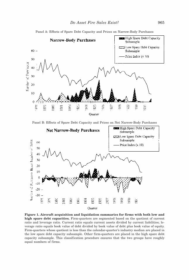
Panel A: Effects of Spare Debt Capacity and Prices on Narrow-Body Purchases

Panel B: Effects of Spare Debt Capacity and Prices on Net Narrow-Body Purchases

Figure 1. Aircraft acquisition and liquidation summaries for firms with both low andhigh spare debt capacities. Firm-quarters are segmented based on the quotient of currentratio and leverage ratio. Current ratio equals current assets divided by current liabilities; le-verage ratio equals book value of debt divided by book value of debt plus book value of equity.Firm-quarters whose quotient is less than the calendar-quarter’s industry median are placed inthe low spare debt capacity subsample. Other firm-quarters are placed in the high spare debtcapacity subsample. This classification procedure ensures that the two groups have roughlyequal numbers of firms.


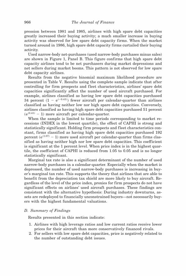
pression between 1981 and 1985, airlines with high spare debt capacitiesgreatly increased their buying activity; a much smaller increase in buyingactivity was observed for low spare debt capacity firms. When the marketturned around in 1986, high spare debt capacity firms curtailed their buyingactivity.

Used narrow-body net-purchases ~used narrow-body purchases minus sales!are shown in Figure 1, Panel B. This figure confirms that high spare debtcapacity airlines tend to be net purchasers during market depressions andnet sellers during market booms. This pattern is not observed for low sparedebt capacity airlines.

Results from the negative binomial maximum likelihood procedure arepresented in Table V. Results using the complete sample indicate that aftercontrolling for firm prospects and f leet characteristics, airlines’ spare debtcapacities significantly affect the number of used aircraft purchased. Forexample, airlines classified as having low spare debt capacities purchased34 percent ~1 2 e~20.41!! fewer aircraft per calendar-quarter than airlinesclassified as having neither low nor high spare debt capacities. Conversely,airlines classified as having high spare debt capacities purchased 51 percent~e~0.41! 2 1! more aircraft per calendar-quarter.

When the sample is limited to time periods corresponding to market re-cessions ~INDEX in the lowest quartile!, the effect of CAPHI is strong andstatistically significant. Holding firm prospects and f leet characteristics con-stant, firms classified as having high spare debt capacities purchased 192percent ~e~1.07! 2 1! more used aircraft per calendar-quarter than firms clas-sified as having neither high nor low spare debt capacities. This coefficientis significant at the 1 percent level. When price index is in the highest quar-tile, the coefficient of CAPHI is reduced from 1.05 to 0.05 and is no longerstatistically significant.

Marginal tax rate is also a significant determinant of the number of usednarrow-body purchases in a calendar-quarter. Especially when the market isdepressed, the number of used narrow-body purchases is increasing in buy-er’s marginal tax rate. This supports the theory that airlines that are able tobenefit from the depreciation tax shield are more likely to buy aircraft. Re-gardless of the level of the price index, proxies for firm prospects do not havesignificant effects on airlines’ used aircraft purchases. These findings areconsistent with the alternative hypothesis: During industry downturns, as-sets are redeployed to financially unconstrained buyers—not necessarily buy-ers with the highest fundamental valuations.

D. Summary of Findings

Results presented in this section indicate:

1. Airlines with high leverage ratios and low current ratios receive lowerprices for their aircraft than more conservatively financed rivals.

2. For sellers with low spare debt capacities, price is negatively related tothe number of outstanding debt issues.


Table V

Maximum Likelihood Estimates for Timing of Used Narrow-Body PurchasesMaximum likelihood estimates presented in this table are based on a Poisson specification with an adjustment to allow for differences betweenthe distribution’s mean and variance. The estimated Variance0Mean ratio equals ~1 1 d!0d. The dependent variable is the number of usednarrow-body aircraft purchased in a calendar-quarter. INDEX is calculated by exponentiating calendar-quarter dummy coefficients in the he-donic pricing model described in equation ~1!:


I

biMODELi 1 (j51

J

bjQTRj 1 (k51

K


where PRICE equals transaction price, MODELi are dummy variables representing aircraft models, QTRj are dummy variables representingcalendar-quarters, STAGEk are dummy variables representing engine stage categories, and AGE equals aircraft age at the time of the transac-tion. High values of INDEX correspond to calendar-quarters where prices are relatively high ~in the sample’s highest quartile!. Low values ofINDEX correspond to calendar-quarters where prices are low ~in the lowest quartile!. CAPLO is a dummy variable equal to 1 if the selling airlinehad a leverage ratio above the industry median and a current ratio below the industry median in the calendar-quarter preceding the transaction;CAPHI is a dummy variable equal to one if the airline had a leverage ratio below the industry median and a current ratio above the industrymedian in the preceding quarter; Q equals market value of equity plus book value of debt divided by book value of equity plus book value of debt;REV equals load factor ~revenue-passenger-miles divided by available-seat-miles! times revenue per revenue-passenger-mile; COST equals cost-of-goods-sold divided by available-seat-miles; t equals the buyer’s marginal tax rate; DELIV equals number of new aircraft deliveries in thecurrent quarter; OWN equals the number of narrow-bodies owned by the airline at the end of the previous quarter. Standard errors are inparentheses.

Dependent Variable 5 Number of Used Narrow-Body PURCHASES per Firm-Quarter

Model CAPLO CAPHI Q REV COST t DELIV log~OWN! Const. log~d!

Complete Sample 20.41 0.41 20.02 213.98 13.16 1.27 20.07 20.15 21.96 21.53~N 5 1027! ~0.238! ~0.188!* ~0.013! ~7.95! ~8.83! ~0.578!* ~0.045! ~0.079! ~0.516!*** ~0.167!***

Low INDEX Quartile 0.27 1.07 0.10 27.18 28.22 2.84 0.01 0.06 22.96 21.71

~N 5 293! ~0.510! ~0.377!** ~0.074! ~16.04! ~17.00! ~1.04!** ~0.060! ~0.192! ~1.33!* ~0.300!***

High INDEX Quartile 20.40 0.05 0.01 219.8 28.0 0.86 20.09 20.11 22.18 21.35

~N 5 272! ~0.417! ~0.367! ~0.018! ~17.76! ~20.82! ~1.21! ~0.088! ~0.163! ~1.06!* ~0.313!***


Do

Asset

Fire

Sales

Exist?

967

3. Prices are lower when buyers are industry outsiders, primarily whenthe used aircraft market is depressed.

4. Firms with low spare debt capacities are more likely to sell to well-financed industry outsiders, especially when the used aircraft marketis depressed.

5. Airlines with high spare debt capacities are more likely to buy aircraftthan those with low spare debt capacities, especially when aircraftprices are depressed.

IV. Alternative Explanation

An alternative explanation for the observed effects of airlines’ financialcharacteristics on price is that financially constrained airlines sell aircraftof lower quality during market depressions. Although the FAA enforces main-tenance requirements, airlines are nevertheless able to choose which air-craft in their f leets to sell. To reduce maintenance expenses, financiallyconstrained airlines may choose to sell aircraft that have little time remain-ing until the next maintenance overhaul. If this is the case, we would expectto see lower transaction prices for financially constrained sellers simply be-cause of quality differences and not because of costs of overcoming capitalmarket imperfections.26 This explanation is consistent with Rose’s ~1990!result that financial health is positively correlated with airline safety. How-ever, it can neither explain the observed relationship between airlines’ sparedebt capacities and levels of used aircraft purchases nor the effect of sellers’financial conditions on buyers’ identities.

To control for aircraft quality differences, one would need information de-scribing the time until next airframe overhaul, the number of hours on theengines, and compliance with FAA Airworthiness Directives for each aircraftat the time of the transaction.27 Unfortunately, these data are generally un-available. Aircraft maintenance records are transferred to aircraft buyers;duplicates are maintained neither by the selling airline nor by the FAA.Thus, the only large-sample data available to control for quality have al-ready been included in the hedonic regression, namely STAGE and AGE.However, quality data are available for a small subsample of Braniff salesthat occurred in April 1984 when that airline was operating under bank-ruptcy court protection. Braniff sold eleven 727-200 ADV aircraft to PeopleExpress, which financed the purchase by issuing secured debt. Included in

26 In extreme cases, financially constrained airlines may fail to properly maintain their air-craft. For example, in an attempt to reduce maintenance expenditures, Eastern Airlines falsi-fied maintenance records on components such as landing gears, wing f laps, and fuel filters.They were eventually found guilty and fined $3.5 million.

27 As the FAA becomes more knowledgeable about causes of aircraft failures, they requirerevisions to air carriers’ maintenance plans. These revisions are called “airworthiness direc-tives.” For example, in response to the failure of the upper section of an Aloha Airlines 737fuselage, the FAA implemented a corrosion prevention program that requires more frequentchecks for airframe deterioration.


the prospectus for this secured debt issue are appraised values for each ofthe eleven Braniff aircraft. Appraised values, which were generated by Av-mark, Inc., an independent aircraft appraisal firm, account for variability inaircraft quality. Based on Avmark’s appraisals, Braniff sold the eleven 727-200 ADVs for an average discount of 32.6 percent. This discount is in excessof the cost of refurbishment incurred by People Express. The estimated dis-count obtained using the hedonic regression methodology is 25 percent. There-fore, based on this small subsample of aircraft, taking quality variation intoaccount would actually increase previously reported discounts.

Even though detailed aircraft quality data are not available in large sam-ple, a test of the hypothesis that quality effects drive discounts at whichairlines sell used aircraft can be performed by repeating the price discountanalysis using sale0leaseback agreements.28 In a typical sale0leaseback agree-ment, an airline sells an aircraft to an investor and immediately leases theaircraft back from the investor. The yield that the investor receives from asale0leaseback transaction depends on both the up-front payment ~the sale0leaseback price! and the magnitude of contracted lease payments. Becausecontracted lease payments are likely to be riskier for financially constrainedlessees, they have to pay a higher yield than their unconstrained rivals.That is, financially constrained airlines will either receive lower up frontpayments and0or make larger periodic lease payments.

Because the airline is responsible for maintaining the aircraft throughoutthe term of the lease, the effect of aircraft quality at lease inception on priceis much smaller for sale0leasebacks than for straight sales. Therefore, ef-fects of financial variables on sale0leaseback prices are likely to be causedby creditworthiness rather than quality considerations. A finding that sale0leaseback prices are correlated with financial variables would refute thehypothesis that the previously documented relationship between sale priceand financial variables is driven by systematic variation in aircraft quality.29

Results from the hedonic regression estimation using only sale0leasebacktransactions are presented in Table A.I, Panel B. The adjusted R2 for thisregression is 0.94 which is greater than the adjusted R2 of 0.76 for straightsale transactions. The increase in R2 for sale0leasebacks may be caused byelimination of quality differences. It may also be caused by the lack of sale0leaseback transactions during used aircraft market depressions, when re-siduals tend to be large. Sale0leasebacks of aircraft models considered inthis paper were virtually nonexistent prior to 1985 but grew rapidly duringthe booming market in the late 1980s. However, when market values forused aircraft declined during late 1990, sale0leaseback agreements were largelylimited to financially healthy airlines—lessors were unwilling to enter long-term lease agreements with financially tenuous lessees.

28 The idea to use sale0leaseback transactions to mitigate quality concerns was suggested byKen Raff, Managing Director of Fleet Transactions at American Airlines.

29 Unfortunately, airlines are only required to disclose the sale0leaseback price ~up frontpayment!. Data on contracted lease payments are not available.


Table VI presents results of estimations of equation ~2! using sale0leaseback transactions. Results are presented both for the entire sampleand for the subsample of transactions that occurred during the 1990–1991 market recession. Consistent with results using straight sale trans-actions, spare-debt-capacity has the biggest effect on sale0leaseback priceduring market recessions. Airlines classified as having high spare debtcapacity receive a 20 percent premium compared to airlines with low andmedium spare debt capacities. This result implies that quality differ-ences do not drive the observed relationship between liquidation priceand financial variables and provides further evidence that financial con-straints are important determinants of prices at which airlines liquidateused aircraft.

Additional support for the conclusion that quality effects are not drivingobserved discounts is obtained by replicating the transaction price analysisafter segmenting the data according to aircraft age. If unobserved aircraftquality is causing the observed relationship between sellers’ financial con-ditions and transaction prices, then, because quality variation is likely to begreater for older aircraft, one would expect the sum of squared residualsfrom price regressions to be greatest when the sample is limited to olderaircraft. To test this conjecture, two subsamples of data are generated. Thefirst subsample contains all narrow-body transactions ~sales, not sale0leasebacks! for which aircraft age is below the sample median. The secondsubsample contains transactions for which aircraft age exceeds the samplemedian. The second specification from Table III is then estimated for eachsubsample. To test whether residuals from the regression using old aircraftare greater than residuals from the regression using young aircraft, theGoldfeld–Quandt Test for heteroskedasticity with respect to age is per-formed. This test fails to reject the null hypothesis of homoskedasticity withrespect to age ~F @197,209# 5 0.775 , F0.05@197,209# 5 1.0!.

Institutional details also help alleviate the concern that quality differ-ences are driving previously reported results. First, costs of aircraft improve-ments ~e.g., engine overhauls, cabin refurbishment! are often reported bybuyers to DOT as part of transaction price. When reported, prices containedin Avmark’s database include these improvement costs. Second, the processof performing major airframe overhauls is carrier-specific. Each U.S. airlineis required by the FAA to have a maintenance plan for every aircraft modelin its f leet. This plan varies across carriers, even for identical aircraft. Thus,for example, if Eastern purchased a 727-200 from United that had just un-dergone a major airframe overhaul, Eastern would still be responsible forperforming maintenance checks required in its own maintenance plan butnot United’s. Eastern would be able to take credit for United’s maintenance,but only to the extent that it can demonstrate to the FAA that United’s planoverlaps Eastern’s. Any work not performed by United but required by theEastern plan would have to be performed by Eastern. For minor mainte-nance checks, this is not likely to be costly. However, for major airframechecks, both the costs of performing additional work as well as costs asso-


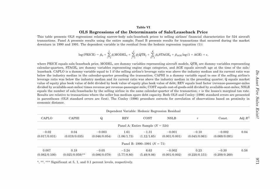
Table VI

OLS Regressions of the Determinants of Sale/Leaseback PriceThis table presents OLS regressions relating narrow-body sale0leaseback prices to selling airlines’ financial characteristics for 524 aircrafttransactions. Panel A presents results using the entire sample; Panel B presents results for transactions that occurred during the marketdownturn in 1990 and 1991. The dependent variable is the residual from the hedonic regression ~equation ~1!!:


I

biMODELi 1 (j51

J

bjQTRj 1 (k51

K


where PRICE equals sale0leaseback price, MODELi are dummy variables representing aircraft models, QTRj are dummy variables representingcalendar-quarters, STAGEk are dummy variables representing engine stage categories, and AGE equals aircraft age at the time of the sale0leaseback. CAPLO is a dummy variable equal to 1 if the selling airline’s leverage ratio was above the industry median and its current ratio wasbelow the industry median in the calendar-quarter preceding the transaction; CAPHI is a dummy variable equal to one if the selling airline’sleverage ratio was below the industry median and its current ratio was above the industry median in the preceding quarter; Q equals marketvalue of equity plus book value of debt divided by book value of equity plus book value of debt; REV equals load factor ~revenue-passenger-milesdivided by available-seat-miles! times revenue per revenue-passenger-mile; COST equals cost-of-goods-sold divided by available-seat-miles; NSLBequals the number of sale0leasebacks by the selling airline in the same calendar-quarter of the transaction; t is the lessee’s marginal tax rate.Results are relative to transactions where the seller has medium spare debt capacity. Both OLS and Conley ~1996! standard errors are presentedin parentheses ~OLS standard errors are first!. The Conley ~1996! procedure corrects for correlation of observations based on proximity ineconomic distance.

Dependent Variable: Hedonic Regression Residual

CAPLO CAPHI Q REV COST NSLB t Const. Adj R2

Panel A: Entire Sample ~N 5 524!

20.02 0.04 20.003 1.61 21.31 20.001 20.10 20.002 0.04~0.01700.031! ~0.01900.035! ~0.04600.054! ~1.0601.73! ~1.1201.65! ~0.00100.001! ~0.04500.061! ~0.06900.091!

Panel B: 1990–1991 ~N 5 71!

0.007 0.18 20.05 23.24 6.63 20.002 0.23 20.30 0.58~0.08200.100! ~0.02500.059!** ~0.08600.079! ~5.7708.80! ~5.4908.06! ~0.00100.002! ~0.22000.151! ~0.20900.260!


Do

Asset

Fire

Sales

Exist?

971

ciated with comparing maintenance plans can be extremely high.30 This pro-vides incentives for airlines to avoid selling aircraft that have recentlyundergone major maintenance checks—regardless of financial condition, air-lines tend to sell planes with few f light-hours remaining until the next air-frame overhaul.

The same argument cannot be made for aircraft engines or airworthinessdirectives. Engines are typically run until there is a problem, at which timethey are overhauled. Financially constrained airlines may face greater in-centives than unconstrained airlines to sell aircraft with many f light hourson the engines or aircraft that have not yet been brought into compliancewith FAA airworthiness directives.

V. Conclusion

This paper estimates discounts at which assets are liquidated by examin-ing prices from a comprehensive sample of commercial aircraft transactions.Use of aircraft transactions has a number of advantages over previouslypublished work on asset liquidation. Not only does it avoid using stock pricereactions to infer costs of liquidation, it also focuses on relatively homo-geneous assets. Furthermore, because the market for used aircraft is ex-tremely liquid compared to markets for most real assets, discounts presentedin this paper represent estimates of lower bounds of liquidation costs. Thesecosts are likely to be greater in industries where used asset markets are lessliquid.

Empirical results presented in this paper are consistent with a model whereprices that sellers accept for their assets depend on costs of raising capital.Airlines with high leverage ratios and low current ratios receive lower pricesfor their assets than more conservatively financed airlines. Furthermore,financially distressed airlines are more likely to sell assets to industry out-siders at low prices. This effect is strongest during market recessions, whencapital constraints limit inside buyers from paying full value for distressedfirms’ assets. Although discounted sales are costly for liquidating firms, theypresent a buying opportunity for conservatively financed firms. The effect ofhigh spare debt capacity on purchasing activity is greatest when aircraftprices are depressed.

These results have important implications for a number of issues in cor-porate finance. First, they suggest benefits from maintaining spare debtcapacity. In addition to avoiding costly liquidation of assets at fire sale prices,maintaining conservative capital structures allows firms to be on the buy-side of industry fire sales. Second, costs of asset liquidation provide a dis-incentive to invest. This may help to explain high capital stock adjustmentcosts noted in the investment0cash f low literature. Finally, findings pre-

30 For example, a major airframe overhaul ~D-Check! for a 737 costs approximately $1 mil-lion. For a 747 airframe, this cost is closer to $5 million ~Source: Mort Beyer, Mort BeyerAssociates!.


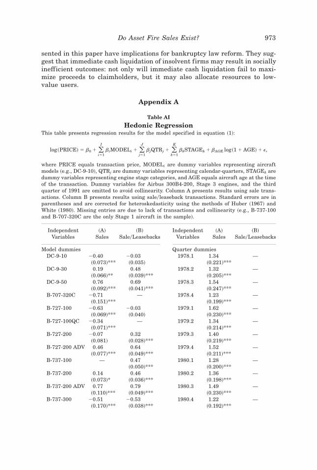
sented in this paper have implications for bankruptcy law reform. They sug-gest that immediate cash liquidation of insolvent firms may result in sociallyinefficient outcomes: not only will immediate cash liquidation fail to maxi-mize proceeds to claimholders, but it may also allocate resources to low-value users.

Appendix A

Table AI

Hedonic RegressionThis table presents regression results for the model specified in equation ~1!:


I

biMODELi 1 (j51

J

bjQTRj 1 (k51

K


where PRICE equals transaction price, MODELi are dummy variables representing aircraftmodels ~e.g., DC-9-10!, QTRj are dummy variables representing calendar-quarters, STAGEk aredummy variables representing engine stage categories, and AGE equals aircraft age at the timeof the transaction. Dummy variables for Airbus 300B4-200, Stage 3 engines, and the thirdquarter of 1991 are omitted to avoid collinearity. Column A presents results using sale trans-actions. Column B presents results using sale0leaseback transactions. Standard errors are inparentheses and are corrected for heteroskedasticity using the methods of Huber ~1967! andWhite ~1980!. Missing entries are due to lack of transactions and collinearity ~e.g., B-737-100and B-707-320C are the only Stage 1 aircraft in the sample!.

IndependentVariables

~A!Sales

~B!Sale0Leasebacks


~A!Sales

~B!Sale0Leasebacks

Model dummies Quarter dummiesDC-9-10 20.40 20.03 1978.1 1.34 —

~0.073!*** ~0.035! ~0.221!***DC-9-30 0.19 0.48 1978.2 1.32 —

~0.066!** ~0.039!*** ~0.205!***DC-9-50 0.76 0.69 1978.3 1.54 —

~0.092!*** ~0.041!*** ~0.247!***B-707-320C 20.71 — 1978.4 1.23 —

~0.151!*** ~0.199!***B-727-100 20.63 20.03 1979.1 1.62 —

~0.069!*** ~0.040! ~0.230!***B-727-100QC 20.34 — 1979.2 1.34 —

~0.071!*** ~0.214!***B-727-200 20.07 0.32 1979.3 1.40 —

~0.081! ~0.028!*** ~0.219!***B-727-200 ADV 0.46 0.64 1979.4 1.52 —

~0.077!*** ~0.049!*** ~0.211!***B-737-100 — 0.47 1980.1 1.28 —

~0.050!*** ~0.200!***B-737-200 0.14 0.46 1980.2 1.36 —

~0.073!* ~0.036!*** ~0.198!***B-737-200 ADV 0.77 0.79 1980.3 1.49 —

~0.110!*** ~0.049!*** ~0.230!***B-737-300 20.51 20.53 1980.4 1.22 —

~0.170!*** ~0.038!*** ~0.192!***


Table AI—Continued


~A!Sales

~B!Sale0Leasebacks


~A!Sales

~B!Sale0Leasebacks

Quarter dummies Quarter Dummies1981.1 1.05 — 1987.2 1.42 0.13

~0.192!*** ~0.206!*** ~0.037!***1981.2 1.16 — 1987.3 1.23 0.18

~0.197!*** ~0.186!*** ~0.036!***1981.3 1.1.4 — 1987.4 1.34 0.17

~0.202!*** ~0.190!*** ~0.038!**1981.4 1.03 0.04 1988.1 1.22 20.59

~0.200!*** ~0.038! ~0.236!*** ~0.217!**1982.1 0.65 — 1988.2 1.28 0.06

~0.226!** ~0.200!*** ~0.044!1982.2 0.95 — 1988.3 1.28 0.11

~0.208!*** ~0.191!*** ~0.037!**1982.3 0.92 — 1988.4 1.17 0.23

~0.223!*** ~0.196!*** ~0.041!***1982.4 0.75 0.09 1989.1 1.14 0.24

~0.240!*** ~0.037!* ~0.195!*** ~0.043!***1983.1 0.88 — 1989.2 1.09 20.31

~0.226!*** ~0.189!*** ~0.038!***1983.2 0.98 — 1989.3 1.20 0.21

~0.202!*** ~0.197!*** ~0.034!***1983.3 0.57 0.10 1989.4 1.24 0.17

~0.220!** ~0.037!** ~0.185!*** ~0.041!***1983.4 0.73 20.16 1990.1 0.96 0.15

~0.194!*** ~0.050!*** ~0.222!*** ~0.041!***1984.1 0.75 20.28 1990.2 1.10 0.23

~0.191!*** ~0.043!*** ~0.192!*** ~0.034!***1984.2 0.90 20.09 1990.3 1.03 20.09

~0.193!*** ~0.044! ~0.203!*** ~0.045!*1984.3 0.94 20.01 1990.4 1.05 0.09

~0.211!*** ~0.038! ~0.214!*** ~0.022!***1984.4 1.00 0.19 1991.1 0.90 0.20

~0.192!*** ~0.048!*** ~0.195!*** ~0.039!***1985.1 1.11 0.11 1991.2 0.69 20.002

~0.190!*** ~0.036!** ~0.214!** ~0.001!1985.2 1.04 0.16 1991.4 20.08 0.38

~0.192!*** ~0.12! ~0.409! ~0.034!***1985.3 1.40 0.07 log~1 1 AGE! 20.16 20.29

~0.193!*** ~0.023!** ~0.057!*** ~0.020!***1985.4 1.31 0.29 St1 Dummy 22.16 —

~0.193!*** ~0.040!*** ~0.277!***1986.1 1.40 0.22 St2 Dummy 21.73 21.56

~0.206!*** ~0.033!*** ~0.146!*** ~0.048!***1986.2 1.08 0.04 Constant 2.83 3.82

~0.243!*** ~0.056! ~0.247!*** ~0.056!***1986.3 1.30 0.15

~0.221!*** ~0.041!***1986.4 1.20 0.18 Number of 1079 621

~0.195!*** ~0.040!*** observations1987.1 1.38 0.10 Adjusted R 2 0.762 0.947

~0.191!*** ~0.038!**

*, **, *** Significant at the 5, 1, and 0.1 percent levels, respectively.


Appendix B

Calculation of Conley (1996) Standard Errors

In their analysis of time series data with autocorrelated disturbances ofunknown structure, Newey and West ~1987! suggest adjusting coefficientstandard errors using the following formula:

V0T 5 ~XT' XT !21F(

t51

T

ut2 xt xt

' 1 (v51

L F1 2v

L 1 1G3 (

t5v11

T

~xt ut ut2v xt2v' 1 xt2vut2vut xt

' !G~XT' XT !21, ~B1!

where X is a matrix of independent variables, xt are vectors of independentvariables, ut is the vector of error terms from the OLS regression, and Lequals the number of researcher-specified lagged periods. The square root ofthe column j, row j element of V/T is the Newey–West ~1987! OLS-estimatorstandard error that accounts for both heteroskedasticity and autocorrela-tion. The weighting factor wij 5 @1 2 v0~L 1 1!#, takes values between zeroand one and assumes that correlation between error terms diminishes as thetime separating observations increases. For example, two observations, i andj, that occurred in consecutive periods are likely to be highly correlated. Aweighting factor close to one would be used for these observations. Con-versely, two observations distant in time would be assumed to be independent—the coefficient standard error weighting factor would be zero for theseobservations. The Newey–West weighting factor declines linearly with thetime between observations for L lags. After L lags, observations are assumedto be independent.

Standard errors presented in this paper follow Conley ~1996! who modifiesthe Newey–West standard error such that weighting factors depend on the“economic distance” ~rather than time! between observations. This is partic-ularly useful when analyzing cross-sectional0time-series data where time isnot necessarily a good measure of the “distance” between observations. Thegeneral idea behind Conley’s approach is that the error term correlation, andtherefore the weighting factor, should increase as economic distance getssmall.

There is a great deal of latitude in specifying both determinants of “eco-nomic distance” and the relationship between these determinants and weight-ing factors. I assume that economic distance between two transactions isshortest when transacting parties are the same, when the aircraft model isthe same, and when the time separating transactions is short. In many cases,airlines sell multiple aircraft to a single buyer on a single date. For thesetransactions, a weighting factor of 1.0 is applied. In contrast, OLS assumesindependence of these observations and applies a weight of zero. A weightingfactor of 0.75 is applied if two transactions have the same seller, occur within


one year of each other, but have different aircraft models or buyers. A weight-ing factor of 0.5 is applied if two transactions have the same seller, regard-less of how much time separates the transactions. As with OLS, a weightingfactor of 1.0 is assigned if i 5 j. All other weighting factors equal zero.Table BI summarizes the weighting scheme used to generate Conley ~1996!standard errors. Because the weighting structure described above assumes ahigh degree of correlation between error terms, Conley’s ~1996! standard errorstend to be much larger than those generated using OLS. The weights havepurposely been chosen in a conservative manner to generate upper boundstandard error estimates. True standard errors are likely to lie somewherebetween the OLS standard errors and the Conley ~1996! standard errors.

Appendix C

Description of Negative-Binomial Model

To model count variables when the variance of the dependent variable issignificantly greater than the mean, Hausman et al. ~1984! suggest modify-ing the Poisson-based likelihood function. The modification involves drop-ping the assumption ~implicit in the Poisson specification! that the Poissonparameter, lit , is a deterministic function of Xit21b. Instead, they assumelit is a gamma-distributed random variable with parameters ~g,d! wheregit 5 exp~Xit21b! and d is constant both across firms and across time. Withthis modification, the variance to mean ratio is:

V~nit !

E~nit !5

1 1 d

d, ~C1!

where d is a parameter to be estimated. The resulting distribution is a neg-ative binomial with probability density function given by:

f ~nit ! 5G~git 1 nit !

G~git !G~nit 1 1! S d

1 1 dDgit

~1 1 d!2nit. ~C2!

Table BI

Conley Standard Errors

Weighting Factor Condition

wij 5 1.0 i 5 jwij 5 1.0 Selleri 5 Sellerj & Buyeri 5 Buyerj & Modeli 5 Modelj & Datei 5 Datej

wij 5 0.75 Selleri 5 Sellerj & |Datei 2 Datej | , 1 yearwij 5 0.50 Selleri 5 Sellerj

wij 5 0.0 Otherwise


Consistent and efficient estimation of this model can be achieved via max-imum likelihood where the appropriate log-likelihood function is:

L~b,d! 5 (1

N

(1

T

@log G~git 1 nit ! 2 log G~git ! 2 log G~nit 1 1!

1 git log~d! 2 git log~1 1 d! 2 nit log~1 1 d!# ~C3!

and

git 5 eXit21 b. ~C4!

Table V presents results using the negative binomial model. Similar resultsare obtained using OLS, indicating that general conclusions are robust tochanges in model specification.

REFERENCES

Aghion, Philippe, Oliver Hart, and John Moore, 1992, The economics of bankruptcy reform, TheJournal of Law, Economics, and Organization 8, 523–546.

Air Carrier Traffic Statistics, 1978–1984, ~Civil Aeronautics Board! and 1985–1991, Depart-ment of Transportation!.

Alexander, Gordon, P. George Benson, and Joan Kampmeyer, 1984, Investigating the valuationeffects of announcements of voluntary corporate selloffs, Journal of Finance 39, 503–517.

Altman, Edward, 1984, A further investigation of the bankruptcy cost question, Journal ofFinance 39, 1067–1089.

Asquith, Paul, Robert Gertner, and David Scharfstein, 1994, Anatomy of financial distress: Anexamination of junk-bond issuers, Quarterly Journal of Economics 109, 625–658.

Baird, Douglas, 1986, The uneasy case for corporate reorganizations, Journal of Legal Studies15, 127–147.

Berndt, Ernst, 1991, The Practice of Econometrics: Classic and Contemporary ~Addison-WesleyPublishing Company, Reading, Mass.!.

Brown, David, Christopher James, and Michael Ryngaert, 1992, Does leverage impede recoveryfrom an earnings shock? An analysis of firms’ responses to poor performance, Unpublishedmanuscript.

Brown, David, Christopher James, and Robert Mooradian, 1994, Asset sales by financially dis-tressed firms, Journal of Applied Corporate Finance 2, 233–258.

Chevalier, Judy, 1995, Debt and product market competition: Local market entry, exit, andexpansion decisions of supermarket chains, American Economic Review 85, 415–435.

Conley, Tim, 1996, Econometric modelling of cross-sectional dependence, Working paper, North-western University.

Cummins, Jason, Kevin Hassett, and R. Glenn Hubbard, 1994, A reconsideration of investmentbehavior using tax reforms as natural experiments, Brookings Papers on Economic Activity,1–74.

Fazzari, Steven, R. Glenn Hubbard, and Bruce Petersen, 1988, Financing constraints and cor-porate investment, Brookings Papers on Economic Activity, 141–195.

Gertner, Robert, and David Scharfstein, 1991, A theory of workouts and the effects of reorga-nization law, Journal of Finance 46, 1189–1222.

Graham, John, 1996a, Debt and the marginal tax rate, Journal of Financial Economics 41,41–73.


Graham, John, 1996b, Proxies for the corporate marginal tax rate, Journal of Financial Eco-nomics 42, 187–221.

Hausman, Jerry, Bronwyn Hall, and Zvi Griliches, 1984, Econometric models for count datawith an application to the patents-R&D relationship, Econometrica 52, 909–938.

Healy, Paul, and Krishna Palepu, 1995, The challenges of investor communication: The case ofCUC International, Inc., Journal of Financial Economics 38, 111–140.

Hite, Gailen, James Owers, and Ronald Rogers, 1987, The market for interfirm asset sales:Partial sell-offs and total liquidations, Journal of Financial Economics 18, 229–252.

Hubbard, R. Glenn, 1995, Capital-market imperfections and investment, Unpublished manuscript.Huber, Peter, 1967, The behavior of maximum likelihood estimates under non-standard condi-

tions, Proceedings of the Fifth Berkeley Symposium on Mathematical Statistics and Prob-ability 1, 221–233.

Jain, Prem, 1985, The effect of voluntary sell-off announcements on shareholder wealth, Jour-nal of Finance 40, 209–224.

Jensen, Michael, and William Meckling, 1976, Theory of the firm: Managerial behavior, agencycosts and ownership structure, Journal of Financial Economics 3, 305–360.

Kim, Moshe, and Vojislav Maksimovic, 1990, Debt and input misallocation, Journal of Finance45, 795–816.

Lang, Larry, Annette Poulsen, and René Stulz, 1995, Asset sales, firm performance, and theagency costs of managerial discretion, Journal of Financial Economics 37, 3–37.

Lerner, Joshua, 1994, Pricing and financial resources: An analysis of the disk drive industry,1980–88, Review of Economics and Statistics 77, 585–598.

Maksimovic, Vojislav, and Gordon Phillips, 1996, Efficiency of bankrupt firms and industryconditions: Theory and evidence, Working paper, University of Maryland.

Moody’s Transportation Manual, 1978–1993.Myers, Stewart, 1977, Determinants of corporate borrowing, Journal of Financial Economics 5,

147–175.Myers, Stewart, 1984, The capital structure puzzle, Journal of Finance 39, 575–592.Myers, Stewart, and Nicholas Majluf, 1984, Corporate financing and investment decisions when

firms have information that investors do not have, Journal of Financial Economics 13,187–221.

Newey, Whitney, and Kenneth West, 1987, A simple positive semi-definite, heteroscedasticityand autocorrelation consistent covariance matrix, Econometrica 55, 703–708.

Opler, Tim, and Sheridan Titman, 1994, Financial distress and corporate performance, Journalof Finance 49, 1015–1040.

Pulvino, Todd, 1996, Effects of bankruptcy court protection on asset sales, Working paper, North-western University.

Rose, Nancy, 1990, Profitability and product quality: Economic determinants of airline safetyperformance, Journal of Political Economy 98, 944–964.

Shleifer, Andrei, and Robert Vishny, 1992, Liquidation values and debt capacity: A market equi-librium approach, The Journal of Finance 47, 1343–1366.

Warner, Jerold, 1977, Bankruptcy costs: Some evidence, Journal of Finance 32, 337–347.Weiss, Lawrence, 1990, Bankruptcy resolution: Direct costs and violation of priority claims,

Journal of Financial Economics 27, 285–314.White, Halbert, 1980, A heteroskedasticity-consistent covariance matrix estimator and a direct

test for heteroskedasticity, Econometrica 48, 817–838.


Documents

Do Asset Fire Sales Exist? An Empirical Investigation of ...piazzesi/Reading/Pulvino 1998.pdf · Do Asset Fire Sales Exist? An Empirical Investigation of Commercial Aircraft Transactions