Do Asian stock market prices follow martingales? Evidence from spectral shape tests

ASIA PACIFIC JOURNAL OF MANAGEMENT VOL 11, NO 2:345-359

DO ASIAN STOCK MARKET PRICES FOLLOW MARTINGALES?

EVIDENCE FROM SPECTRAL SHAPE TESTS

Fong Wai Mun and Koh Seng Kee*

This paper examines the martingale hypothesis for five Asian stock markets using the spectral shape tests of DurIauf (1991). Unlike the variance ratio test employed in previous studies (eg, Pan et al, 1991), the spectral shape tests' are consistent against all stationary alternatives to the martingale null.

The spectral shape tests were applied to daily and weekly returns on the stock indices of Thailand, Hang Kong, Korea, Malaysia and Taiwan over a period of 17 years'. The results show that the martingale null is rejected for most markets. There is some evidence that the rejections may be due to low frequency or long memory influences.

1. INTRODUCTION 1

Asian stock markets have made impressive strides in recent years in line with the rapid growth of their economies. Yet, compared with the vast body of research on Anglo-Saxon stock markets, very little is known about the behaviour of these emerging markets. Recent exceptions to this include studies by Bailey et al (1990) and Pan et aI (1991). Both of these studies investigate whether Asian stock markets behave as martingales.

The martingale hypothesis states that asset returns are serially uncorrelated at all leads and lags. This hypothesis has received a long-standing interest in finance, partly because the martingale property is an implication of many models of rational asset pricing, 1 but also because rejections of the martingale hypothesis may suggest alternative ways to model the stochastic behaviour of asset prices.

In this paper, we test the martingale hypothesis using data on five Asian stock markets. They are Thailand, Hang Kong, Korea, Malaysia and Taiwan. We study daily stock prices spanning ten years for all five countries, and also weekly prices running up to 17 years for some countries. Bailey et al (1990) examine the martingale hypothesis for nine Asia-

* The authors are lecturers, Department of Finance and Banking, National University of Singapore. This paper was presented at the Third International Conference on Asian-Pacific Financial Markets, September 9-11, 1993 in Singapore. We have benefited greatly from the comments of Y K Tse and other conference participants.

1. See for example, Hall (1978), Lucas (1978) and Shiller (1981).

345

Do Asian Stock Market Prices Follow Martingales? Evidence from Spectral Shape Tests

Pacific markets with up to eight years of daily data. They do not examine weekly returns, which is quite important if infrequent or thin trading is a serious problem in these emerging markets. Furthermore, some of the stock indices employed by Bailey et al are equally weighted, and thus more susceptible to infrequent trading biases. We reduce such biases by using only returns on value-weighted market portfolios. Pan et al (1991) study both daily and weekly returns but their sample period is just 41/2 years. Large sample sizes are crucial in many tests of the martingale null since these tests lack power when the sample size is small (eg, Lo, 1989, 1991).

Most tests of the martingale null are in the time domain. For example, Bailey et al

(1990) focus on the statistical significance of return autocorrelations over short lags. Pan et al (1991) apply the variance ratio test of Cochrane (1988) and Lo and MacKinlay (1988), which can roughly be interpreted as a test of weighted summed autocorrelations over a specified number of lags.

There is evidence that conventional autocorrelation-based tests such as the Box-Pierce Q or Ljung-Box statistic are neither very reliable nor powerful compared to the variance ratio test, against a number of alternatives to the martingale null (Lo, 1989). However, there are major drawbacks in using the variance ratio test. Asymptotic sampling theory for the variance ratio requires that the differencing interval or lag goes to infinity as the sample size goes to infinity (Campbell and Mankiw, 1987). As explained below, this implies that the variance ratio test is not consistent against all alternatives to the null but only against those processes with slow decaying or persistent autocorrelations such as mean-reverting rime-series. Thus the variance ratio test implicitly assumes that high frequency deviations from the null are unimportant.

In some situations, we might want to test the martingale hypothesis against broad classes of alternatives, and perhaps follow the analysis up by testing the null against specific alternatives. This would appear to be an appropriate strategy for studying the behaviour of Asian stock markets, since relatively little is known about their time-series properties. In this paper, we employ a family of frequency domain "spectral shape" tests which allows us to implement this test strategy. Unlike the variance ratio test, the spectral shape tests are asymptotically consistent against all alternatives of the martingale null. Thus, spectral shape tests do not ignore information at high frequencies. Yet, the tests are flexible enough to enable the researcher to focus on deviations from the null at specific ranges of frequencies. For example, if the data suggest the presence of long memory in stock prices, the spectral shape tests can be directed against long memory alternatives by focusing on the behaviour of the spectrum at frequencies near zero.

This paper is organised as follows. In Section 2, we survey some recent variance ratio tests of the martingale hypothesis for stock markets. Section 3 introduces the spectral shape tests and compares them with the variance ratio test. Section 4 contains a description of the data used in this study to test the martingale hypothesis. The results of the spectral shape tests for our sample are reported in Section 5. These results are compared with those obtained from the variance ratio test. Section 6 provides some interpretations of our findings. Section 7 concludes the paper.

346

APJM

2. VARIANCE RATIO TEST

The variance ratio methodology has been used in many recent empirical studies on the behaviour of financial asset prices (eg, Lo and MacKinlay, 1988; Poterba and Sum- mers, 1988) The use of this methodology was motivated by the idea that in an informationally inefficient market, prices could take long but temporary swings from their "fundamental" values, perhaps due to fads. In the time domain, this hypothesis implies that asset returns exhibit mean reversion ie, they are positively correlated over short horizons and negatively correlated over long horizons. In the frequency domain, mean reversion implies that the martingale null can be rejected at low frequencies, perhaps due to the presence of long- range dependence or long memory in stock returns (see Lo, 1991). By construction, conventional autocorrelation-based tests such as the Box-Pierce Q statistic may not be powerful against long-term mean reversion unless distant autocorrelations are large) The variance ratio test was developed partly to overcome this problem.

The variance ratio test is both simple and intuitively appealing. The test exploits the fact that if a time-series is a martingale, then the variance of the q-th difference of the series is q times the variance of the first-difference. Thus, if asset prices follow a martingale process, the variance of the q-period holding returns should be equal to q times the variance of the one-period returns. In other words, the following variance ratio should equal one:

1 (y2(rq) V(q) = q ~2(r-- ~ - (1)

where (y2(rq) and o2(r) are the variance of the q-period and one-period holding returns respectively. Lo and MacKinlay (1988) applied the variance ratio test to weekly and monthly CRSP NYSE-AMEX stock returns data from 1962-85. They reject the martingale null for weekly returns and find that the variance ratio generally exceeds one for holding periods of less than 16 weeks. The same pattern of variance ratio is found for monthly returns, although the null cannot be rejected. Using monthly CRSP NYSE data from 1926- 85, Poterba and Summers also reject the null hypothesis, but in contrast to Lo and MacKinlay they find that variance ratios are generally less than one at lags beyond a year. Overall, the results of these studies suggest that stock returns are positively autocorrelated over short lags, followed by negative autocorrelations over longer lags. Contrary to the martingale hypothesis, it appears that US stock prices may contain a mean reverting component] The variance ratio test has also been applied to other stock markets. For example, Pan et al (199t) compute variance ratios of up to 20 lags for six Asian stock market indices using daily and weekly data. They find that for daily data, the martingale hypothesis can be rejected at 5% across most lags in three markets (Hong Kong, Singapore and Korea). Evidence against the null is much weaker for weekly returns, with the variance ratio significantly different from one at most lags for only one country, namely Taiwan.

2. For example, both the Box-Pierce and Ljung-Box statistics sum the squares of autocorrelations at all specified lags. Thus, unless the autocorrelations at long lags are large, these statistics may have low power against long-term mean reversion.

3. However, Kim et al (1991) dispute this conclusion, and provide evidence to show that for the US stock market, mean reversion is found only for the post-World War II period.

347

Do Asian Stock Market Prices Follow Martingales ? Evidence from Spectral Shape Tests

A key drawback of the variance ratio test is that it is not consistent against all alternatives to the martingale hypothesis. This is because the variance ratio test focuses only on zero frequency ie, long memory behaviour of a time-series. Consequently, high frequency deviations of the alternative from the null are ignored. To elaborate, we follow Cochrane (1988) and express the variance ratio as follows:

q-1

V ( q ) - l + 2 ~ ( 1 - j ^ " q) p(./) (2) j=l

where p(j) is the jth order sample autocorrelation of x t, a martingale difference sequence. FNuation (2) says that the variance ratio is approximately equal to one plus the weighted sum of the first q- 1 sample autocorrelations where the weights decline linearly with time lags. The weighted sum in equation (2) can be readily interpreted in the frequency domain.

Let f0~) denote the normalised spectral density function of x, at frequencies )~.

1 f(~) = ~ ~p( j )cos(~j ) (3)

Thus, under the hypothesis of no serial correlation at all leads and lags, f(~) is a constant equal to 1Am Given a sample of T observations, a consistent estimate of the normalised spectral density function is as follows:

k-1

Ik(~) -- 1 £ ( 1 - k)~(j)cos()~j) (4) ~.2 2r¢ j=-(k-1)

I k ()v) where ~ is the normalised periodogram estimated by truncating the sample at k < T and

(1 - J ) is the familiar zero frequency Bartlett window (see, eg, Priestley, 1981, p 439).

Comparing equations (2) with (4), it is clear that the variance ratio is proportional to an estimate of the normalised spectral density function at zero frequency using a Bartlett window. This estimate will be consistent provided k --+ ~ as T --+ ~o and k/T --> (Priestley, 1981, p 433).

From the above discussion, we see that the variance ratio test focuses only on zero frequency deviations of the spectral shape from that under the martingale null. In other words, the test is not consistent against all non-white noise departures from the null but only against those with long memory characteristics. However, if our goal is to test the general implications of the martingale hypothesis, then tests which make use of information at all frequencies will be more appropriate. The spectral shape tests described in the next section avoid the problem of specificity associated with the variance ratio test.

3. S P E C T R A L S H A P E T E S T S

As noted in the previous section, the spectral density function is a constant under the martingale null. This suggests that tests of the martingale hypothesis can be based on deviations of the sample spectral density function from the null. The following statistic suggested by Durlauf (199 t) provides a basis for constructing useful test statistics:

348

APJM

gt II > t .l, 0

Here, UT(t) denotes the cumulative deviations of the normalised sample periodogram from the null. Notice that we make use of the cumulative periodogram deviations rather than simply periodogram deviations, because it is well known that the periodogram is an inconsistent estimate of the spectral density function. Consequently, the periodogram deviations will not converge to a rectangle. In contrast, the cumulative deviations will converge under the null, due to the averaging of individual frequency estimates.

The above spectral shape test stands in rather sharp contrast to the variance ratio test. Whereas consistent estimates of the variance ratio statistic focus only on zero frequency deviations of the spectral density function from the null, the UT(t) statistic detects deviations from the null at all frequencies in the range [0,n]. Thus, the spectral shape tests are appropriate for testing the martingale hypothesis against broad classes of alternatives. For the remainder of this paper, we will employ several test statistics based on UT(t) to test the following composite null hypothesis (Durlauf, 1991, p 358):

Ho: Heteroscedastic Martingale Null Hypothesis

(1) E(xtk~t_l) = ~t where ~ is the cy algebra generated by xk, k < j.

(2) E(xt2)= 02.

T

(3) lira T-1 ~ E (xj~l,~j_l) = ry 2 >0 almost surely. T-->~

j=l

(4) There exists a random variable W with finite E(W 4) such that P(Ixjl>g) <c P(IWl>g) for some 0 < c < ~ and all j, all g>_0.

(5) E(xj2Xj_rXj_s) = k(r,s) finite and uniformly bounded Vj, r_>l and s_>l.

T

(6) lira T -1 ~xj,~xj_+ E(x+21~ 1) = k(r,s) almost surely. T--->~

j=l+min(r,s)

(7) E(xj 8) is uniformly bounded Vj.

A detailed discussion of this composite null can be found in Durlauf (1991, p 358). Briefly, Condition 1 is the null hypothesis, namely that x, is a martingale difference sequence. Since there is substantial empirical evidence that financial time-series exhibit time-varying volatilities (Baillie and Bollerslev, 1989), there is a need to ensure that the test is robust to general forms of heteroscedasticity. Conditions 2 through 6 allow for some degree of heterogeneity whilst still permitting the application of (functional) central limit theorems. 4 Condition 7 characterises the behaviour of the sample periodogram but is not needed in the development of the asymptotic theory.

4. Very similar conditions were used by Lo and MacKinlay (1988) in developing a heteroscedastic- robust version of their variance ratio test, except that they also allow for weak dependence in the time-series.

349


Multiplying equation (5) by ~/2T 1/2, we can re-express UT(t ) as:

= ~ T g b ( j ) sinjnt t e [0,1] (6) --;- j=l )

Equation (6) is now simil~ in form to a representation of a Brownian bridge on the unit interval. Four statistics which are based on the Brownian bridge can be used to test the null hypothesis:

(1) Anderson-Darling (AD) Statistic:

1

l" Ur (t) 2 - a D r = J ~ c t t (7)

0

(2) Cramer-von Mises (CMV) Statistic:

1

= [ U r (t) 2 dt (8) CVMr ¢lJ

0

(3) Kolmogorov-Smirnov (KS) Statistic:

KS r = suplU~(t)l (9) t ~ [0,1]

(4) Kuiper Statistic:

Kr = suplUr(t) - Ur(.s)l (10) [0 < s,t < 11

Limiting empirical distributions of the four statistics have been tabulated by Shorack and Wellner (1987). Finite sample distributions of the statistics for T=1000 are given in Durlauf (1991, p 368). There are, as yet, few studies of the finite sample properties of the above test statistics. However, simulation evidence by Durlauf (1990) confirms that for independent normal errors, the CMV statistic has "good" size properties.

To compute the spectral test statistics, spectral windows are applied to smooth the raw periodogram which is otherwise an inconsistent estimate of the true spectral density function. We use two admissible windows: Bartlett and Parzen. Theorem 3.1 of Durlauf (1991, p 365) assures asymptotic equivalence of window-based to periodogram-generated spectral shape tests. There are no fixed rules regarding the choice of window span, although a Common rule of thumb is ~ (Chatfield, 1985). We therefore use two other window spans: 2 "~fT and 3 ~@- as a check on result sensitivity.

4. DATA

The data used in this paper are daily and weekly returns on value-weighted portfolios of five markets: Thailand, Korea, Hong Kong, Malaysia and Taiwan. The data are obtained from the Pacific-Basin Capital Markets (PACAP) database of the University of Rhode Island, US. All returns are computed as the first-difference of the natural log of stock price

350

APJM

which includes dividends. Daily returns span the ten years from January 1982 to December 1991. The average number of daily observations for the five markets is 2559. Weekly returns are calculated using Wednesday-to-Wednesday closing prices. The weekly sample sizes range from 591 to 877, Details of the samples are shown in Table 1:

TABLE 1 DESCRIPTION OF DATA

Market Market Index Period of Daily Returns Period of Weekly Returns (Sample Size) (Sample Size)

Thailand

Hong Kong

Korea

Malaysia

Taiwan

Stock Exchange of Thailand Thailand Index Hang Seng Index

Korea Composite Stock Price Price Index Kuala Lumpur Composite Index Taiwan Stock Exchange Weighted Stock Price Index

4.t.82 - 30.12.91 (2461)

4.1.82-31.12.91 (2471)

4,1.82 - 26,12.91 (2927)

4.1.82- 18.5.90 (2052)

5.1,82 - 28.12.91 (2878)

7.5.75 - 12.12.91 (821)

9,1.80- 18.12.91 (591)

5.1.77 - 18.12.91 (877)

5.1.77 - 16.5.90 (655)

8.1.75 - 18.12.91 (876)

5. RESULTS

Table 2 presents descriptive statistics in the form of daily autocorrelations of the five returns series for up to 20 lags. The first order autocorrelation coefficient of each series is positive and significant, as are a number of distant autocorrelation coefficients. Thus, it appears that the returns series are not white noise.

Table 3 summarizes the results of the variance ratio test for the daily data. In Table 3, variance ratios of up to 64 days (ie, q = 64) are reported. Under the null hypothesis of no serial correlation, the variance ratio is asymptotically normally distributed with mean equals to one, thus allowing the application of a standard z test. Since there is evidence that many financial time-series display time-varying volatilities (Baillie and Bollerslev, 1989), we compute heteroscedasfic-adjusted test z statistics which are reported in parentheses under each variance ratio. The adjustment for heteroscedasticity is via Theorem 3 of Lo and MacKinlay (1988) which allows for a variety of time-varying volatilities including deterministic changes in variance (eg, due to seasonal factors) and Engle's (1982) ARCH process in which the conditional variance depends on past variance and random shocks.

Table 3 shows that the null hypothesis can be rejected for all five daily returns series at the 5% level. The variance ratio significantly differs from one across all specified lags for Thailand and Taiwan and for most lags in the case of Malaysia and Korea. Thus, for these markets, the null can be firmly rejected. For Hong Kong, the evidence against the null is weaker as the variance ratio is significantly different in only two out of six lags. Table 3 also reveals two other features of the sample variance ratios. First, all the variance ratios exceed one and second, their magnitude generally increases with the lag. This pattern of the variance ratio is consistent with the predominantly positive autocorrelations which we

351

Do Asian Stock Market Prices Follow Martingales? Evidence fi'om Spectral Shape Tests

TABLE 2 AUTOCORRELATIONS OF DALLY RETURNS

Lag Autocorrelation coefficients

Thailand Hong Kong Korea Malaysia Taiwan

1 2 3 4 5 6 7 8 9

10 11 12 13 t4 15 16 17 18 19 20

0.214" 0.058* 0.061" 0.077*

-0.035 -0.013 -0.041

0.001 0.021 0,036 0.002 0,046* 0.054* 0.025 0.044*

-0.008 0,014 0.005

-0.040 0.001

0.086* 0,023 0,108" 0.025

-0,004 -0.017

0,072* 0.033

-0.007 0.013 0.011 0.009

-0.014 -0.017 -0.050* -0.045*

0.004 -0.023 -0,014

0.004

0.110" -0.033

0.006 0.016 0.024

-0.020 -0.030 -0.018

0.027 -0.023

0,017 0,O28 0.031 0.044* 0.043*

-0.023 0.010 0.022 0.026 0.004

0.127" 0.054* 0,063*

-0.010 0,077*

-0.012 -0.006

0.010 0.015 0.028 0.061" 0,012 0.002 0.028

-0,030 0.004

-0.011 0.033 0.019 0.000

0.163' 0.023 0.126" 0,056* 0,012

-0.009 0.012

-0.006 0.015 0,050* 0.057* 0.032 0.058* 0.019 0.030 0.045* 0.000

-0.031 0,039 0,004

* denotes that the absolute value of the corresponding autocorrelation coefficient is more than two times the standard error, The standard error is computed using Bartlett's (1946) approximation as follows:

1/n 1 + 2~r3 z where 13 is the jth-order autocorrelation coefficient and q is the number of lags.

TABLE 3 VARIANCE RATIOS OF DAILY STOCK PRICES

Market:

Thailand

Hong Kong

Korea

Malaysia

Taiwan

Lags (q)

1.21 (4,09**) 1.09

(1,23) 1.11

(3.94**) 1.13

(1,47) 1.16

(5,33**)

4

1.41 (4.32**) 1.21

(1.84) 1.13

(2.54*) 1.28

(1,84) 1.33

(5,71"*)

1.59 (4.02**) 1.35

(2.34*) 1.16

(1.98") 1.42

(1.98") 1.54

(5,88**)

16

1,71 (3.68**) 1.50

(2,55*) 1.18

(1.67) 1.59

(2,15") 1.78

(5,74**)

32

1.96 (3.74**) 1.43

(1.76) 1.29

(1,94) 1.77

(2,38*) 2,03

(5.30**)

64

2,15 (3.37**) t.29

(0.97) 1.34

(1.70) 1.96

(2.54*) 2,22

(4.46**)

Variance ratios are gaven in the man rows. Figures in parentheses refer to heteroscedastic-consistent z statistics, ** (*) indicate that the corresponding variance ratio is statistically different from one (null hypothesis) at (1%) 5%,

352

APJM

saw earlier in Table 2. It is also the pattern found by Lo and MacKinlay (1988) for US

weekly and monthly returns as well as by Pan et aI (1991) for daily and weekly returns of Asian stock markets over short holding periods. Similar to these studies, our variance ratio test indicates that the null is rejected not on account of mean reversion, but rather because of positive dependence in the returns.

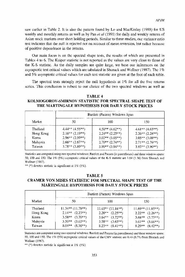
Our main focus is on the spectral shape tests, the results of which are presented in Tables 4 to 6. The Kuiper statistic is not reported as the values are very close to those of the K-S statistic. As the daily samples are quite large, we base our inferences on the asymptotic test critical values which are tabulated in Shorack and Wel lner (1987). The 1%

and 5% asymptotic critical values for each test statistic are given at the foot of each table.

The spectral tests strongly reject the null hypothesis at 1% for all the five returns series. This conclusion is robust to our choice of the two spectral windows as well as

TABLE 4 K O L M O G O R O V - S M I R N O V STATISTIC FOR SPECTRAL SHAPE TEST OF

THE MARTINGALE HYPOTHESIS FOR DAILY STOCK PRICES

Bartlett (Parzen) Windows Span

Market 50 100 150


4.44** (4.55**) 2.16"* (2.19"*) 2.96** (2.99**) 2.66** (2.67**) 3.78** (3.89**)

4.58** (4.62**) 2.24** (2.25**) 3.02** (3.05**) 2.70** (2.74**) 3.90** (3.94**)

4.61"* (4.65**) 2.26** (2.28**) 3.05** (3.08**) 2.71"* (2.76**) 3.93** (3.96**)

Statistics are computed using two spectral windows: Bartlett and Parzen (in parentheses) and three window spans: 50, t00 and 150. The 1% (5%) asymptotic critical values of the K-S statistic are 1.64 (1,36) from Shorack and Wellner (t987). ** (*) denotes statistic is significant at 1% (5%).

TABLE 5 CRAMER VON MISES STATISTIC FOR SPECTRAL SHAPE TEST OF THE

MARTINGALE HYPOTHESIS FOR DAILY STOCK PRICES


Market 50 100 150


11.34"* (11.78"*) 2.14"* (2.23**) 3.58** (3.70**) 3.50** (3.63**) 8.04** (8.36**)

11.63"* (11.84"*) 2.20** (2.25**) 3.64** (3.72**) 3.58** (3.65**) 8.23** (8.41"*)

11.69'* (l 1.85"*) 2.22** (2.26**) 3.68** (3.73**) 3.61"* (3.66**) 8,29** (8.42**)

Statistics are computed using two spectral windows: Bartlett and Parzen (in parentheses) and three window spans: 50, 100 and 150. The 1% (5%) asymptotic critical values of the CMV statistic are 0.46 (0.74) from Shorack and Wellner (1987). ** (*) denotes statistic is significant at 1% (5%).

353


TABLE 6 ANDERSON-DARLING STATISTIC FOR SPECTRAL SHAPE TEST OF THE

M A R T I N G A L E HYPOTHESIS FOR DAILY STOCK PRICES


Market 50 100 150


57.50** (59.80**) 13.08"* (13.70"*) 17.91"* (18.52"*) 19.35"* (20.16"*) 45.38** (47.35**)

59.58** (60.70**) 13.79"* (14.17"*) 18.44"* (18.85"*) 20.24** (20.77**) 47.49** (45.70**)

60.27** (61.10"*) 14.01"* (14.306"*)

18.64"* (18.93"*) 20.66** (20.99**) 45.31"* (49.23**)

Statistics are computed using two spectral windows: Bartlett and Parzen (in parentheses) and three window spans: 50, 100 and 150. The 1% (5%) asymptotic critical values of the AD statistic are 2A9 (3.86) from Shorack and Wellner (1987). ** (*) denotes statistic is significant at 1% (5%).

window lengths. Compared to the variance ratio test, the spectral shape tests seem to provide firmer evidence against the martingale null. This result is not entirely surprising since, as mentioned earlier, the spectral shape tests are asymptotically powerful against all stationary non-white noise alternatives to the martingale null, whereas the variance ratio test is not.

To check whether the above results are merely due to the October 1987 global stock market crash, we performed variance ratio and spectral shape tests on modified samples with returns omitted over the few days surrounding Wall Street's "mini-crash" of October 14 and the global stock market crash following October 19. 5 The results for the modified samples (not reported) are generally the same as before. Thus, events surrounding the October 1987 crash cannot be responsible for the rejections of the null.

However, rejections of the null may be due to positive autocorrelations induced by infrequent trading of some index component stocks (see Scholes and Williams, 1977). It is well known that smaller capitalisation stocks tend to be more thinly and infrequently traded than larger stocks. Thus, new information is likely to be impounded first on the prices of large stocks, followed by those of smaller stocks. Stale prices for smaller stocks can in turn artificially induce positive autocorrelation in the returns of a portfolio consisting mostly of such stocks. For obvious reasons, the problem caused by infrequent trading is likely to be more severe with daily data, although our use of value-weighted as opposed to equally weighted market portfolios should help to reduce any bias caused by infrequent trading. To reduce this bias further, we ran the above tests again using weekly returns on value- weighted portfolios. Table 7 shows the results of the variance ratio test for the weekly data. Results of the spectral shape tests based on the Bartlett window with a window span of

5. The omitted days in October 1987 are as follows: 19-21 for Thailand, Korea and Taiwan, 19, 20 and 22 for Malaysia (21 October was a holiday in Malaysia) and 19 and 26 for Hong Kong (the market was closed after 19 October and resumed trading only on 26 October).

354

T A B L E 7

V A R I A N C E R A T I O S O F W E E K L Y S T O C K P R I C E S

APJM

Market:

Thailand

Hong Kong

Korea

Malaysia

Taiwan

Lags (q)

2 4 8 16 32

1.13 -(2.03*)

1.09 (1.32) 1.01

(0.15) 1.09

(1.68) 0.98

(-0.42)

1.29 (2.40*) 1.18

(1.57) 1.00

(0.03) 1.26

(2.51") 1.01

(0.15)

1.49 (2.71"*) 1.13

(0.73) 1.02

(0.14) 1.43

(2.73**) 1.04

(0.29)

1.67 (2.60**) 1.01

(O.O3) 1.06

(0.35) 1.57

(2.49*) 1.08

(0.48)

1.72 -(2.06")

0.77 (-0.74)

1.16 (0.68) 1.52

(1.68) 1.17

(0.71)

Variance ratios are given in the main rows. Figures in parentheses refer to heteroscedastic-consistent z statistics. ** (*) indicate that the corresponding variance ratio is statistically different from one (null hypothesis) at 1% (5%).

T A B L E 8 S P E C T R A L S H A P E T E S T O F T H E M A R T I N G A L E H Y P O T H E S I S F O R

W E E K L Y S T O C K P R I C E S

Market


Test Statistics

K-S

1.79" 1.18" 0.90 1.41" 0.59

Kuiper

1.80" 1.40 1.60 1.66" 0.83

CMV

1.49" 0.42 0.20 0.70* 0.07

AD

8.08* 1.91 1.40 3.99* 0.4t

Statistics are computed using a Bartlett window with the window span of 2 ~q;. The 5% finite sample test critical values are: (1) K-S:I.16 (2) Kuiper:l.60 (3) CMV:0.49 and (4) AD:3.14 from Durlauf (1991). * denotes statistic is significant at 5%.

2~/-T-T are summarized in Table 8. Separate tests performed with Parzen windows and different window spans do not materially affect the results, and are omitted from Table 8.

Based on the variance ratio test, we see that there is now less extensive evidence against the null hypothesis. Specifically, at the 5% level, we can reject the null across all five lags only for Thailand. We can also reject the null for Malaysia but only for three out of the five lags. The null is not rejected for the other three markets. Of these, the result for Taiwan bears mention. The non-rejection of the null for Taiwan using weekly returns is in direct contrast with strong rejections for daily returns, suggesting that infrequent trading may be responsible for the daily result.

355

Do Asian Stock Market Prices Follow Martingales ? Evidence from Spectral Shape Tests

Table 8 shows that broadly similar inferences are obtained from the spectral shape tests based on finite sample critical values derived from Monte Carlo simulations (see Durlauf, 1991, p 368). 6 To the extent that weekly sampling is able to significantly reduce non-trading bias, the findings suggest that rejections of the null for Thailand and Malaysia cannot be mainly attributed to non-trading effects. 7 In other words, stock prices in these markets do not appear to exhibit martingale behaviour.

6. INTERPRETATION OF RESULTS

W~hile both the variance ratio and spectral shape tests reject the null, they do not point to specific alternatives concerning the stochastic processes of daily and weekly stock prices. Nonetheless, two important clues can be picked up from the results. First, returns in our sample are highly positively autocorrelated even at fairly long lags, and this rules out simple mean-reverting processes such as those entertained by Summers (1986) or Fama and French (1987), where stock prices are assumed to contain a random walk and a stationary mean-reverting component. As Fama and French (1987) point out, such processes imply that returns are not only negatively autocorrelated over all holding periods, but that up to a point, the degree of negative autocon'elation increases with the length of the holding period. This prediction is not borne out in our data.

Second, as is well known from the work of Granger (1980) and Granger and Joyeux (1980), persistent autocorrelations may be a symptom of long memory influences on returns. The spectral shape tests (particularly the AD and CMV statistics) are well suited for detecting long memory effects, since the spectral densities of long memory processes are either zero or unbounded at zero frequency, whereas they are finitely bounded in the presence of short memory. If long memory is present, this should result in a much larger value for the AD statistic relative to the CMV statistic. As shown in Tables 4 to 6, this indeed is the case for both the daily and weekly samples, suggesting that returns may have long memory components.

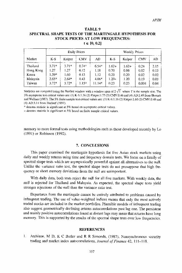
It is also possible to perform the spectral shape tests over low frequencies so as to maximise power against long memory alternatives. We therefore computed all four spec: tral shape statistics over arbitrarily low frequencies, specifically for t ~ (0, 0.2). The results of this test, presented in Table 9, provide some evidence that low frequency components of the returns are indeed the main source of rejections of the null. This is, of course, not a rigorous test. A natural extension of this paper would be to subject the hypothesis of long

6. Note that Durlauf's simulated finite sample critical values are for a fixed sample size of 1000, and thus do not exactly match the sample sizes studied by us.

7. Furthermore, simple but plausible models of infrequent trading often predict returns autocorrelations which decay much faster than those observed in our daily and weekly samples (cf Table 2). For example, Lo and MacKinlay (1988) formulate a binomial model in which the probability (p) of a security being not traded in any given period and find that the returns autocorrelations of an equally weighted portfolio of such securities decay as p(1-p)~. Thus, even if on average 50% of securities do not trade in any given period, it is easy to see that the autocon-elations become close to zero beyond five lags. See also Perry (1985) and Atchison et al (1987).

356

APJM

TABLE 9 SPECTRAL SHAPE TESTS OF THE MARTINGALE HYPOTHESIS FOR

STOCK PRICES AT LOW FREQUENCIES: t ~ [0, 0.2]

Market


Daily Prices

K-S Kuiper CMV AD

3.71" 3.71" 0.74* 6.54* 1.27 1.27 0.12 1.18 1.59" 1.60 0.13 1.12 2.65* 2.64* 0.43 4.06* 3.72* 3.72* 1.15" 11.14"

Weekly Prices

K-S Kuiper CMV AD

1.62+ t.62+ 0.24 2.15 0.70 0.86 0.02 0.13 0.20 0.20 0.02 0.02 1.20+ 1.20 0.19 0.03 0.23 0.23 0.004 0.04

Statistics are computed using the Bartlett window with a window span of 2 ~ where T is the sample size. The 5% asymptotic test critical values are: (1) K-S:1.36 (2) Kuiper:l.75 (3) CMV:0.46 and (4) AD:2.49 from Shorack and Wellner (1987). The 5% finite sample test critical values are: (1) K-S: t. 16 (2) Kuiper: 1.60 (3) CMV:0.49 and (4) AD:3.14 from Durlauf (1991). * denotes statistic is significant at 5% based on asymptotic critical values. + denotes statistic is significant at 5% based on finite sample critical values.

memory to more formal tests using methodologies such as those developed recently by Lo (1991) or Robinson (1992).

7. CONCLUSIONS

This paper examined the martingale hypothesis for five Asian stock markets using daily and weekly returns using time and frequency domain tests. We focus on a family of spectral shape tests which are asymptotically powerful against all alternatives to the null. Unlike the variance ratio test, the spectral shape tests do not presuppose that high frequency or short memory deviations from the null are unimportant.

With daily data, both tests reject the null for all five markets. With weekly data, the null is rejected tor Thailand and Malaysia. As expected, the spectral shape tests yield stronger rejections of the null than the variance ratio test.

Departures from the martingale cannot be entirely attributed to problems caused by infrequent trading. The use of value-weighted indices means that only the most actively traded stocks are included in the market portfolios. Plausible models of infrequent trading also suggest geometrically declining returns autocorrelations past lag one. The persistent and mainly positive autocorrelations found at distant lags may mean that returns have long memory. This is supported by the results of the spectral shape tests over low frequencies.

1.

REFERENCES

Atchison, M D, K C Butler and R R Simonds, (1987), Nonsynchronous security trading and market index autocorrelations, Journal of Finance 42, 111-118.

357


2. Bailey, W, R M Stulz and S Yen, (1990), Properties of daily stock prices from the Pacific-Basin stock markets: Evidence and implications, S G Rhee and R P Chang (eds), Pacific-Basin Capital Markets Research, VoI 1, North-Holland: Netherlands.

3. Baillie, R T and T Bollerslev, (1989), Common stochastic trends in a system of exchange rates, Journal of Finance 44, 167-181.

4. Bartlett, M S, (1946), On the theoretical specification and sampling properties of autocorrelated time series, Journal of the Royal Statistical Society (supplement), 8, 27-85.

5. Campbell, J Y and N G Mankiw, (1987), Are output fluctuations transitory? Quarterly Journal of Economics 102, 857-880.

6. Chatfield, C, (1985), The Analysis of Time Series, 3rd ed, London: Chapman and Hall.

7. Cochrane, J, (1988), How big is the random walk in GNP? Journal of Political Economy 96, 893-920.

8. Durlauf, S N, (1990), Time series properties of aggregate output fluctuations, Working Paper, Stanford University, Stanford, CA.

9. Durlauf, S N, (1991), Spectral based testing of the martingale hypothesis, Journal of Econometrics 50, 355-376.

10. Engle, R, (1982), Autoregressive conditional heteroscedasticity with estimates of the variance of United Kingdom inflation, Econometrica 50, 987-1007.

11. Fama, E, (1970), Efficient capital markets: A review of theory and empirical work, Journal of Finance 25,383-417.

12. Fama, E, (1991), Efficient capital markets: II, Journal of Finance 46, 1575-1617.

13. Fama, E and K French, (1988), Permanent and transitory components of stock prices, Journal of Political Economy 96, 246-273.

14. Granger, C W, (1980), Long memory relationships and the aggregation of dynamic models, Journal of Econometrics 14, 227-238.

15. Granger, C W and R Joyeux, (1980), An introduction to tong memory time series models and fractional differencing, Journal of Time Series Analysis 1, 15-29.

16. Hall, R, (1978), Stochastic implications of the life-cycle-permanent income hypothesis: Theory and evidence, Journal of Political Economy 86, 971-987.

17. Ito, K and H P McKean, (1974), Diffusion Processes and Their Sample Paths, Springer-Verlag: Berlin.

18. Kim, M J, C R Nelson and R Startz, (1991), Mean reversion in stock prices? A reappraisal of the empirical evidence, Review of Economic Studies 58, 515-528.

19. LeRoy, S, (1973), Risk aversion and the martingale property of stock returns, Interna- tional Economic Review 14, 436-446.

20. LeRoy, S, (1989), Efficient capital markets and martingales, Journal of Economic Literature 27, 1583-1621.

21. Lo, A W and C MacKinlay, (1988), Stock market prices do not follow random walks: Evidence from a simple specification test, Review of Financial Studies 1, 41~56.

358

APJM

22. Lo, A W and C MacKinlay, (1989), The size and power of the variance ratio test in finite samples: A Monte Carlo investigation, Journal of Econometrics 40, 203-238.

23. Lo, A W, (1991), Long-term memory in stock market prices, Econometrica 59, 1279- 1313.

24. Lucas, R, (1978), Asset prices in an exchange economy, Econometrica 46, 1429- 1446.

25. Pan, M S, J R Chiou, R Hocking and H K Kim, (1991), An examination of mean- reverting behaviour of stock prices in Pacific-Basin stock markets, in SG Rhee and RP Chang (eds), Pacific-Basin Capital Markets Research, Vol 2, North-Holland: Nether- lands.

26. Perry, P P, (1985), Portfolio serial correlation and nonsynchronous trading, Journal of Financial and Quantitative Analysis 20, 517-523.

27. Phillips, P C B and P Perron, (1988), Testing for a unit root in time series regression, Biometrika 75, 335-346.

28. Poterba, J and L Summers, (1988), Mean reversion in stock returns: Evidence and implications, Journal of Financial Economics 22, 27-60.

29. Priestley, M B, (1981), Spectral Analysis and Time Series, Academic Press: London.

30. Robinson, P M, (1992), Log periodogram regression of time series with long range dependence, Mimeo, London School of Economics.

31. Shiller, R, (1981), Do stock prices move too much to be justified by subsequent changes in dividends? American Economic Review 71, 42t-436.

32. Shorack, G R and J A Wellner, (1987), Empirical Processes with Applications to Statistics, Wiley: New York, NY.

33. Summers, P, (1986), Does the stock market rationally reflect fundamental values? Journal of Finance 41,591-601.

359

Documents

Do Asian stock market prices follow martingales? Evidence from spectral shape tests