Embed Size (px)
Citation preview
1
DNN Accelerator Architectures
ISCA Tutorial (2019)Website: http://eyeriss.mit.edu/tutorial.html
Joel Emer, Vivienne Sze, Yu-Hsin Chen
2
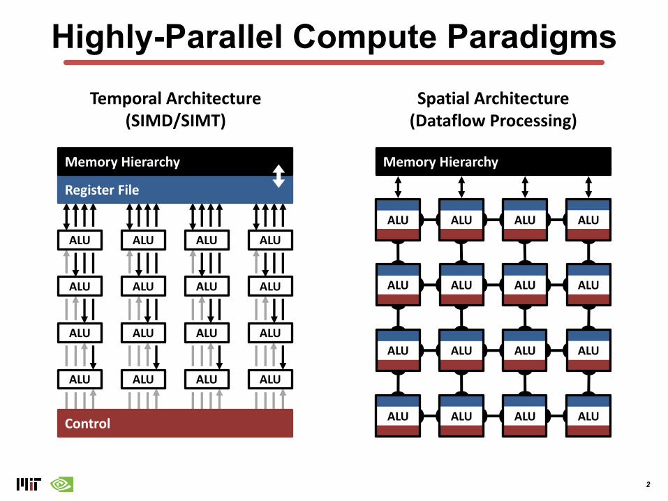
Highly-Parallel Compute ParadigmsTemporal Architecture
(SIMD/SIMT)Spatial Architecture
(Dataflow Processing)
Register File
Memory Hierarchy
ALU
ALU
ALU
ALU
ALU
ALU
ALU
ALU
ALU
ALU
ALU
ALU
ALU
ALU
ALU
ALU
Control
Memory Hierarchy
ALU ALU ALU ALU
ALU ALU ALU ALU
ALU ALU ALU ALU
ALU ALU ALU ALU
3
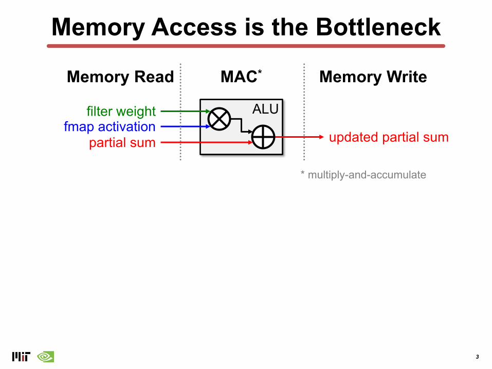
Memory Access is the Bottleneck
ALUfilter weightfmap activation
partial sum updated partial sum
Memory Read Memory WriteMAC*
* multiply-and-accumulate
4
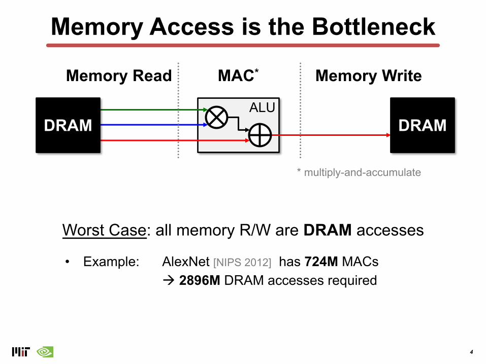
Memory Access is the Bottleneck
ALU
Memory Read Memory WriteMAC*
* multiply-and-accumulate
DRAM DRAM
• Example: AlexNet [NIPS 2012] has 724M MACs à 2896M DRAM accesses required
Worst Case: all memory R/W are DRAM accesses
5
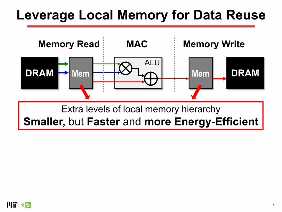
Leverage Local Memory for Data Reuse
ALU
Memory Read Memory WriteMAC*
MemDRAM DRAMMem
Extra levels of local memory hierarchySmaller, but Faster and more Energy-Efficient
6
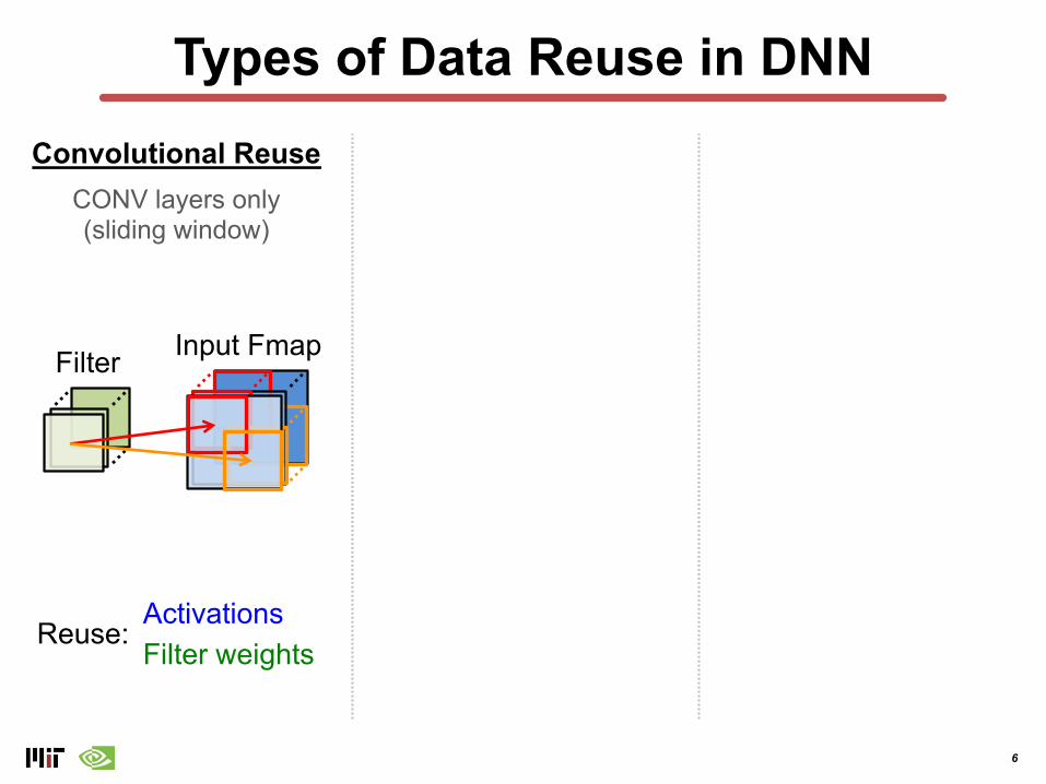
Types of Data Reuse in DNNConvolutional Reuse
CONV layers only(sliding window)
Filter Input Fmap
ActivationsFilter weights
Reuse:
7
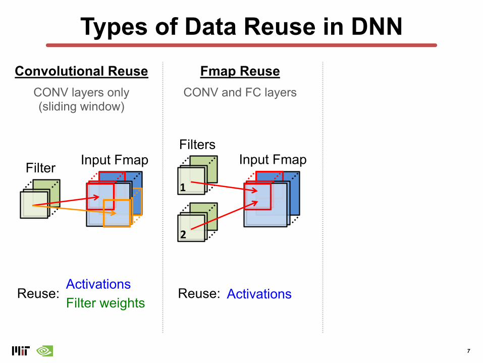
Types of Data Reuse in DNNConvolutional Reuse Fmap Reuse
CONV layers only(sliding window)
CONV and FC layers
Filter Input FmapFilters
2
1
Input Fmap
ActivationsFilter weights
Reuse: ActivationsReuse:
8
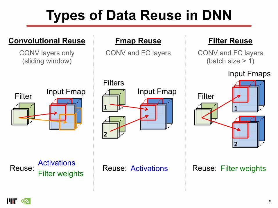
Types of Data Reuse in DNNFilter ReuseConvolutional Reuse Fmap Reuse
CONV layers only(sliding window)
CONV and FC layers CONV and FC layers(batch size > 1)
Filter Input FmapFilters
2
1
Input Fmap Filter
2
1
Input Fmaps
ActivationsFilter weights
Reuse: ActivationsReuse: Filter weightsReuse:
9
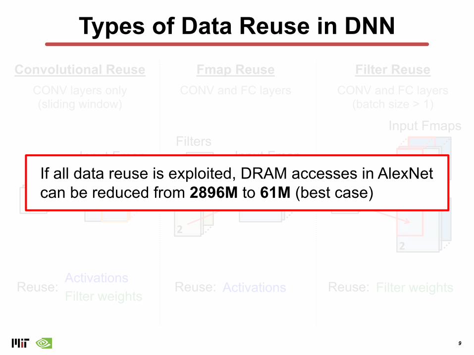
Types of Data Reuse in DNNFilter ReuseConvolutional Reuse Fmap Reuse
CONV layers only(sliding window)
CONV and FC layers CONV and FC layers(batch size > 1)
Filter Input FmapFilters
2
1
Input Fmap Filter
2
1
Input Fmaps
ActivationsFilter weights
Reuse: ActivationsReuse: Filter weightsReuse:
If all data reuse is exploited, DRAM accesses in AlexNet can be reduced from 2896M to 61M (best case)
10
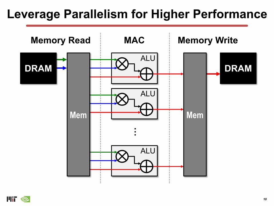
Leverage Parallelism for Higher Performance
Memory WriteMAC
DRAM DRAMALU
Memory Read
ALU
ALU
…
MemMem
11
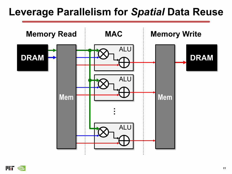
Leverage Parallelism for Spatial Data Reuse
Memory WriteMAC
DRAM DRAMALU
Memory Read
ALU
ALU
…
MemMem
12
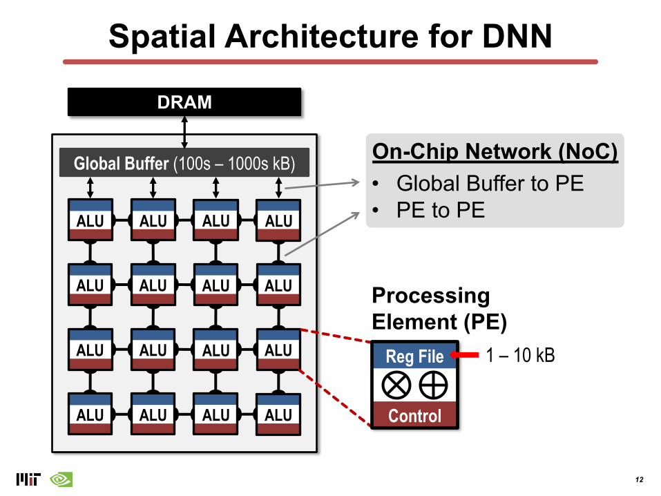
Spatial Architecture for DNN
ProcessingElement (PE)
Global Buffer (100s – 1000s kB)
ALU
ALU
ALU
ALU
ALU
ALU
ALU
ALU
ALU
ALU
ALU
ALU
ALU
ALU
ALU
ALU
DRAM
Control
Reg File 1 – 10 kB
On-Chip Network (NoC)• Global Buffer to PE• PE to PE
13
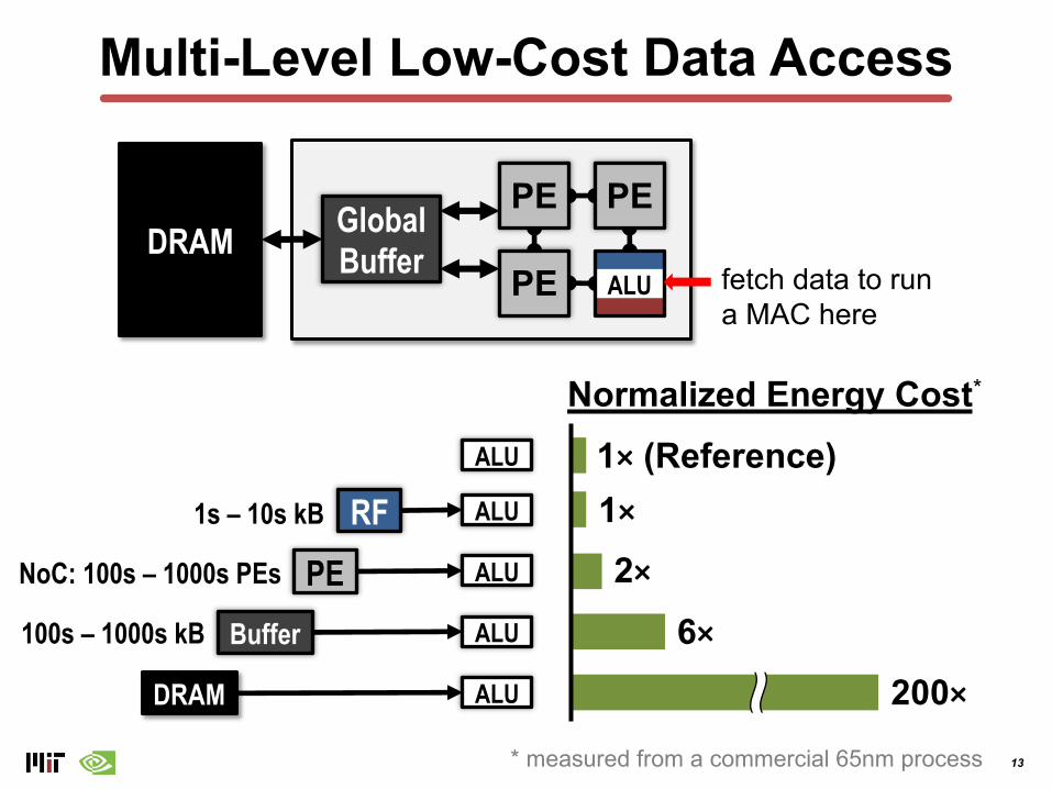
Multi-Level Low-Cost Data Access
DRAM GlobalBuffer PE
PE PE
ALU fetch data to run a MAC here
ALU
Buffer ALU
RF ALU
Normalized Energy Cost*
200×6×
PE ALU 2×1×1× (Reference)
DRAM ALU
1s – 10s kB
100s – 1000s kB
NoC: 100s – 1000s PEs
* measured from a commercial 65nm process
14
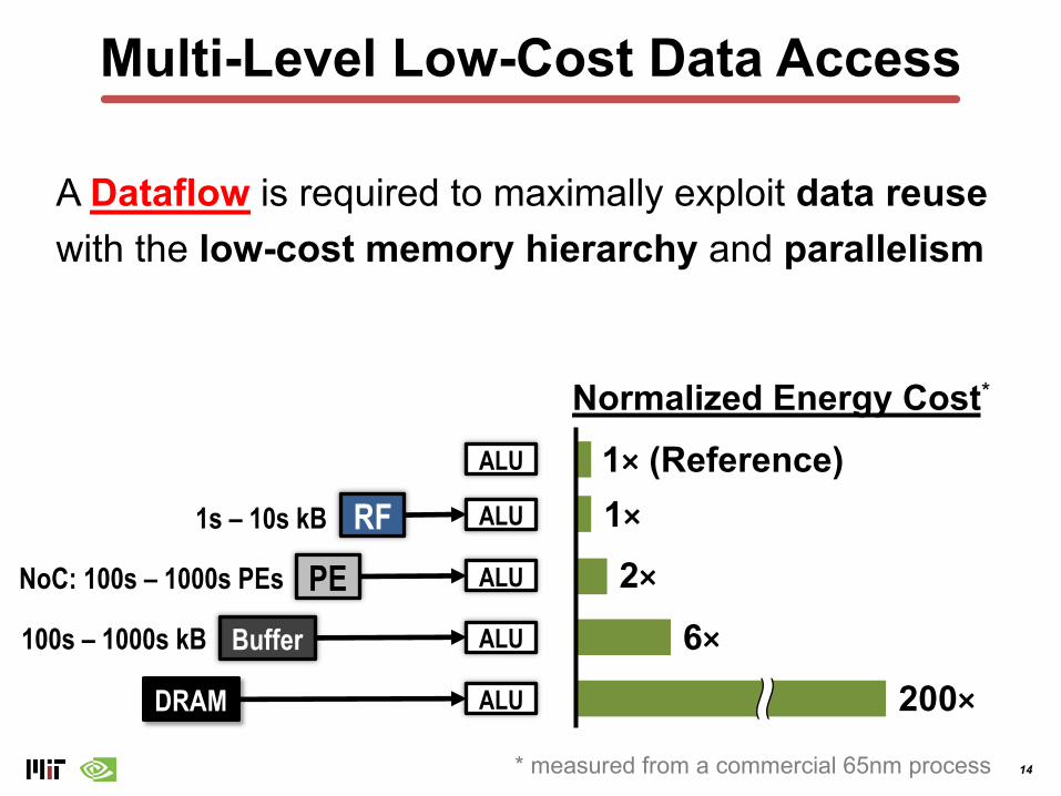
Multi-Level Low-Cost Data Access
ALU
Buffer ALU
RF ALU
Normalized Energy Cost*
200×6×
PE ALU 2×1×1× (Reference)
DRAM ALU
* measured from a commercial 65nm process
1s – 10s kB
100s – 1000s kB
NoC: 100s – 1000s PEs
A Dataflow is required to maximally exploit data reuse with the low-cost memory hierarchy and parallelism
15
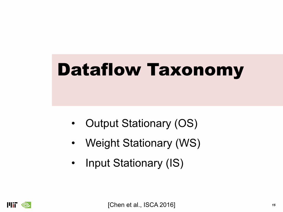
Dataflow Taxonomy
• Output Stationary (OS)
• Weight Stationary (WS)
• Input Stationary (IS)
[Chen et al., ISCA 2016]
16
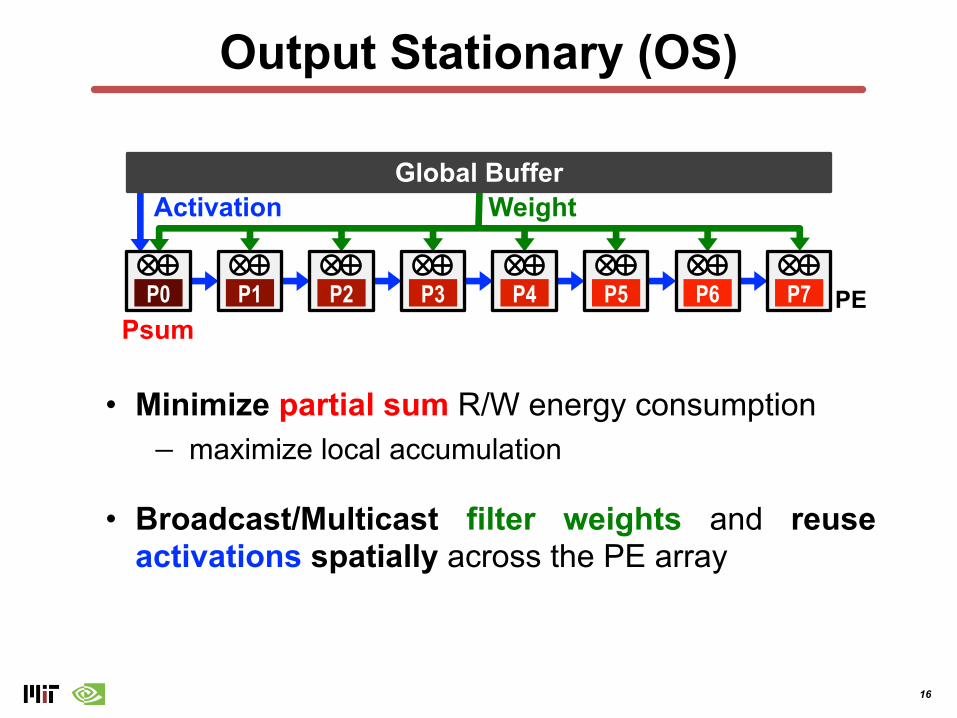
• Minimize partial sum R/W energy consumption− maximize local accumulation
• Broadcast/Multicast filter weights and reuseactivations spatially across the PE array
Output Stationary (OS)
Global Buffer
P0 P1 P2 P3 P4 P5 P6 P7
Activation Weight
PEPsum
17
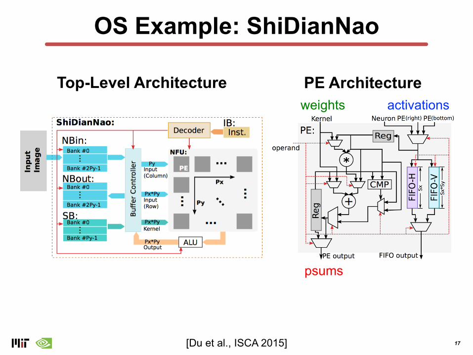
OS Example: ShiDianNao
Top-Level Architecture PE Architecture
[Du et al., ISCA 2015]
weights activations
psums
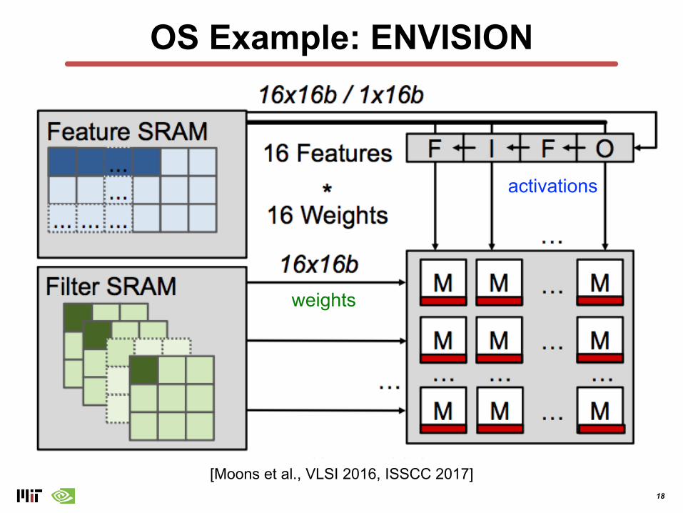
18
OS Example: ENVISION
[Moons et al., VLSI 2016, ISSCC 2017]
weights
activations
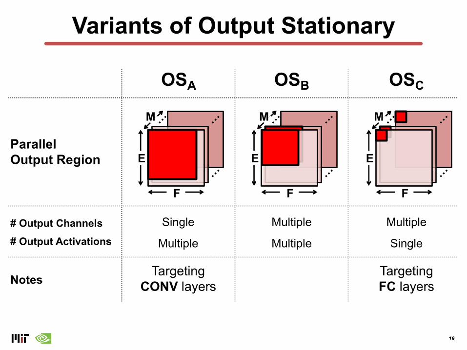
19
Variants of Output Stationary
# Output Channels# Output Activations
E
F
…
…
…M
OSB
Multiple
Multiple
Notes
E
F
…
…
…M
OSA
Single
Multiple
TargetingCONV layers
E
F
…
…
…M
OSC
Multiple
Single
TargetingFC layers
Parallel Output Region
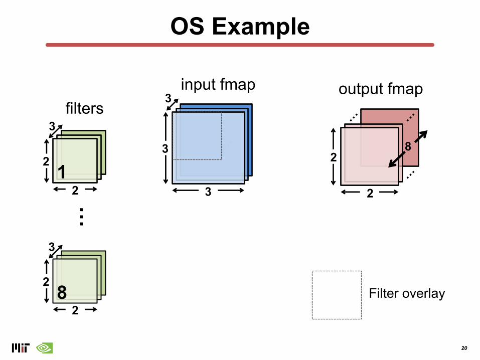
20
OS Example
…
2
output fmap
…
…filters
8
…
2
21
2
3
3
input fmap
…
3 2
3
3
Filter overlay82

21
OS Example
…
2
output fmap
…
…
…
2
21
2 8
3
3 2
input fmap3
3
3
2
8
filters
1
8
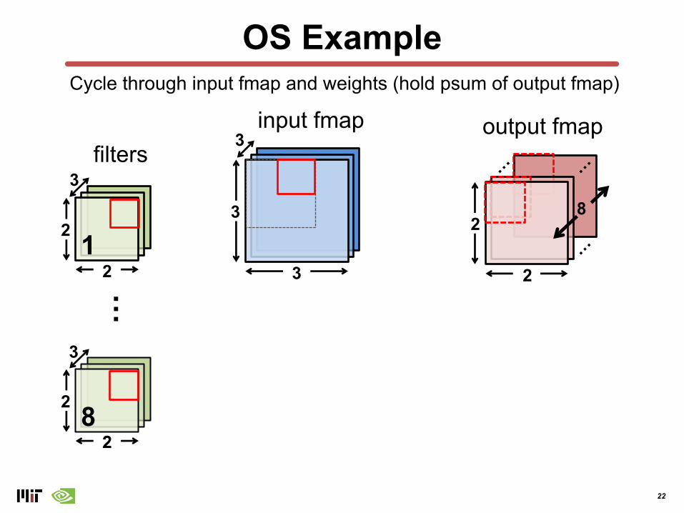
Cycle through input fmap and weights (hold psum of output fmap)
Incomplete partial sum
22
OS Example
input fmapCycle through input fmap and weights (hold psum of output fmap)
3
3
3…
2
output fmap
…
…
2
8
2
…
2
21
2 8
3
3
2
filters
1
8

23
OS Example
…
2
21
28
input fmap
3
3
2
3
3
3filters
1
…
2
output fmap
…
…
2
8
Cycle through input fmap and weights (hold psum of output fmap)
8

24
OS Example
…
2
21
2
input fmap
3
3
2
3
3
3filters
1
…
2
output fmap
…
…
2
8
Cycle through input fmap and weights (hold psum of output fmap)
8

25
OS Example
…
2
output fmap
…
…
…
2
21
2 8
3
3 2
input fmap3
3
3
2
8
filters
1
8
Cycle through input fmap and weights (hold psum of output fmap)
26
OS Example
…
2
output fmap
…
…
…
2
21
2 8
3
3 2
input fmap3
3
3
2
8
filters
1
8
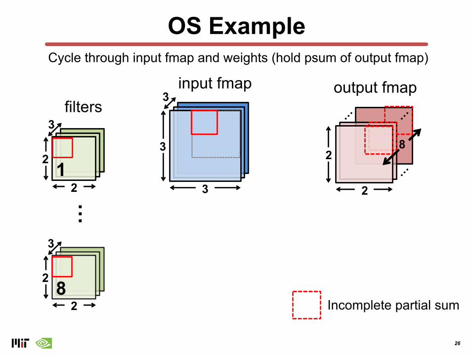
Cycle through input fmap and weights (hold psum of output fmap)
Incomplete partial sum
27
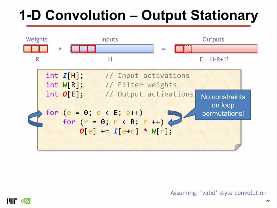
1-D Convolution – Output Stationary
R
Weights
H
Inputs
E = H-R+1†
Outputs
* =
int I[H]; // Input activationsint W[R]; // Filter weightsint O[E]; // Output activations
for (e = 0; e < E; e++)for (r = 0; r < R; r ++)
O[e] += I[e+r] * W[r];
† Assuming: ‘valid’ style convolution
No constraints on loop
permutations!
28
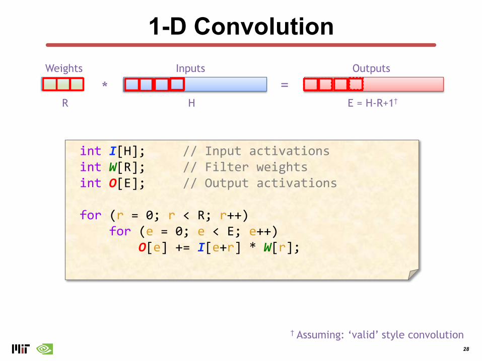
1-D Convolution
R
Weights
H
Inputs
E = H-R+1†
Outputs
* =
int I[H]; // Input activationsint W[R]; // Filter weightsint O[E]; // Output activations
for (r = 0; r < R; r++) for (e = 0; e < E; e++)
O[e] += I[e+r] * W[r];
† Assuming: ‘valid’ style convolution
29
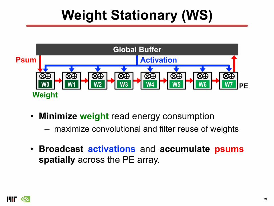
Weight Stationary (WS)
• Minimize weight read energy consumption− maximize convolutional and filter reuse of weights
• Broadcast activations and accumulate psumsspatially across the PE array.
Global Buffer
W0 W1 W2 W3 W4 W5 W6 W7
Psum Activation
PEWeight
30
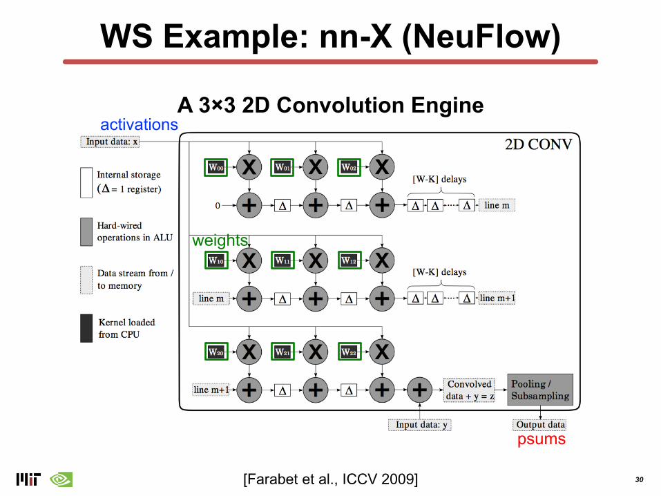
WS Example: nn-X (NeuFlow)
[Farabet et al., ICCV 2009]
A 3×3 2D Convolution Engine
weights
activations
psums
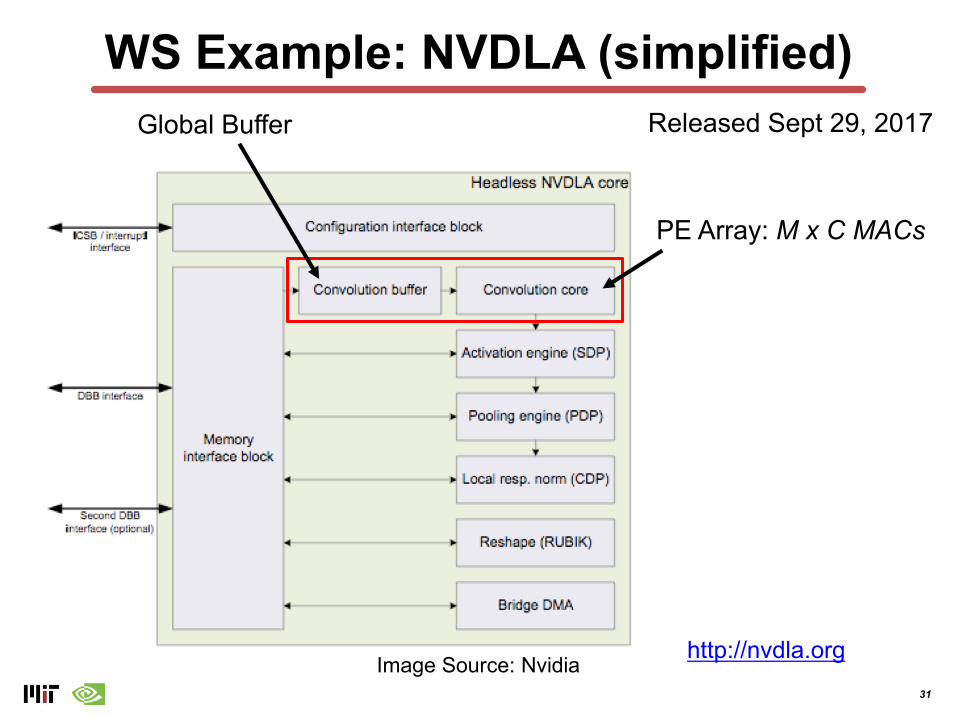
31
Image Source: Nvidia
Released Sept 29, 2017Global Buffer
PE Array: M x C MACs
http://nvdla.org
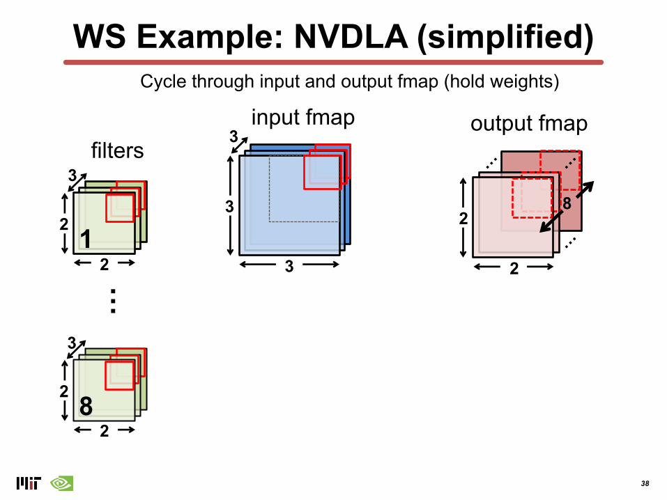
WS Example: NVDLA (simplified)
32
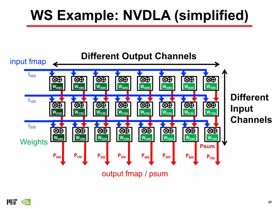
WS Example: NVDLA (simplified)
Different Output Channels
DifferentInputChannels
I000
P000
W0000 W1000 W2000 W3000 W4000 W5000 W6000 W7000
W0100 W1100 W2100 W3100 W4100 W5100 W6100 W7100
W0200 W1200 W2200 W3200 W4200 W5200 W6200 W7200
P100 P200 P300 P400 P500 P600
Psum
P700
I100
I200
output fmap / psum
input fmap
Weights
33
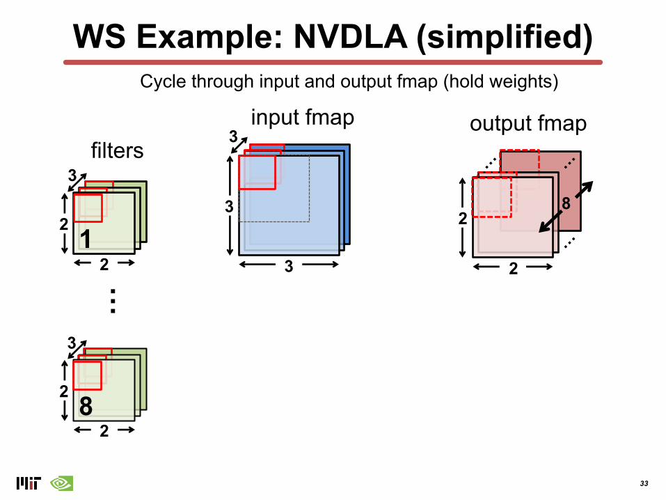
WS Example: NVDLA (simplified)
…
2
output fmap
…
…
…
2
21
2 8
3
3 2
input fmap3
3
3
2
8
filters
1
8
Cycle through input and output fmap (hold weights)
34
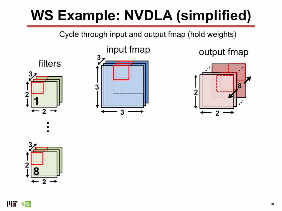
WS Example: NVDLA (simplified)
…
2
output fmap
…
…
2
input fmapCycle through input and output fmap (hold weights)
3
3
3
8
…
2
21
2 8
3
3
2
filters
1
8

35
WS Example: NVDLA (simplified)
output fmap…
2
21
2 8
input fmap
3
3
2
Cycle through input and output fmap (hold weights)
3
3
3…
2…
…
2
8
filters
1
8
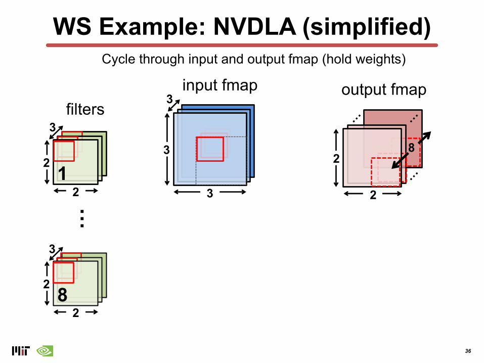
36
output fmapinput fmapCycle through input and output fmap (hold weights)
3
3
3…
2…
…
2
8
…
2
21
2 8
3
3
2
filters
1
8
WS Example: NVDLA (simplified)
37
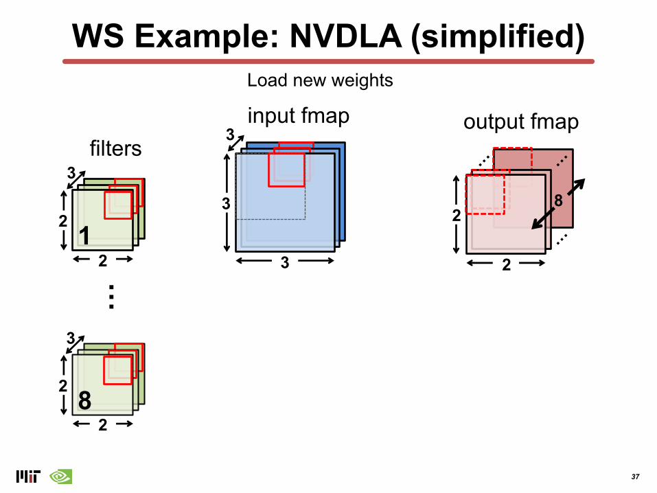
WS Example: NVDLA (simplified)
output fmapinput fmapLoad new weights
3
3
3…
2
21
2 8
3
3
2
filters
1
8
…
2…
…
2
8
38
WS Example: NVDLA (simplified)
output fmapinput fmap
3
3
3
Cycle through input and output fmap (hold weights)
…
2…
…
2
8
…
2
21
2 8
3
3
2
filters
1
8
39
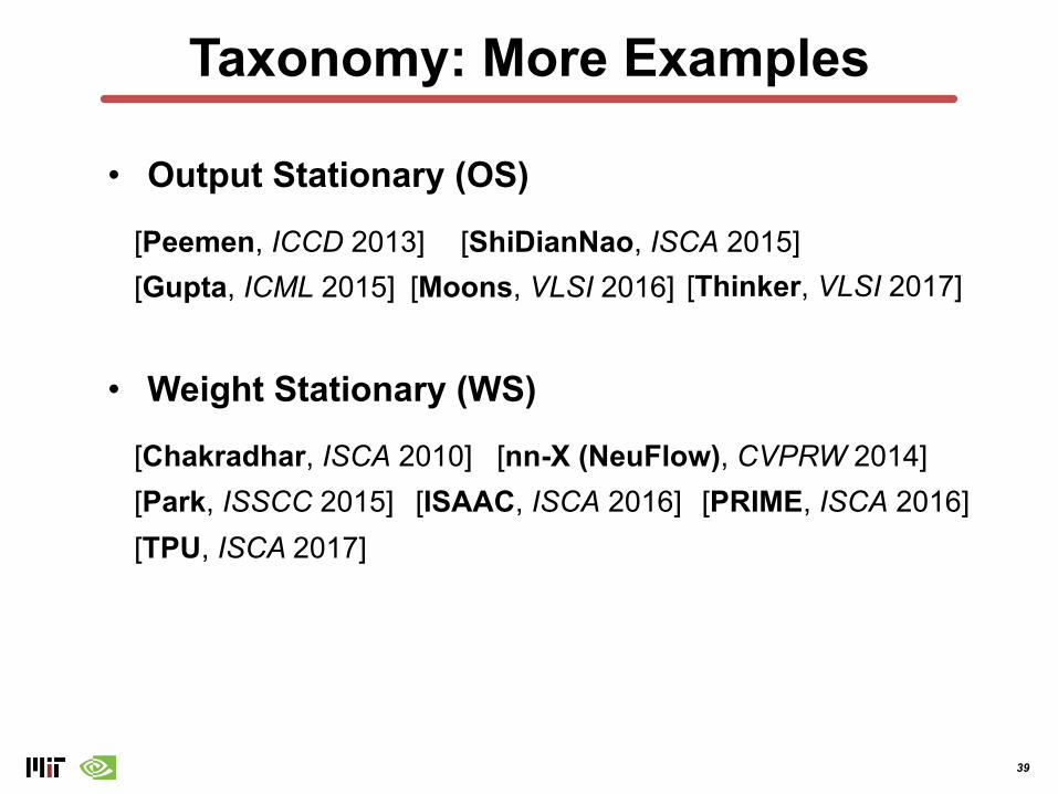
Taxonomy: More Examples
• Weight Stationary (WS)
[Chakradhar, ISCA 2010] [nn-X (NeuFlow), CVPRW 2014][Park, ISSCC 2015] [ISAAC, ISCA 2016] [PRIME, ISCA 2016]
• Output Stationary (OS)
[ShiDianNao, ISCA 2015][Peemen, ICCD 2013][Gupta, ICML 2015] [Moons, VLSI 2016] [Thinker, VLSI 2017]
[TPU, ISCA 2017]
40
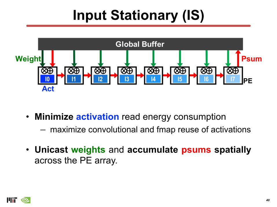
Input Stationary (IS)
• Minimize activation read energy consumption− maximize convolutional and fmap reuse of activations
• Unicast weights and accumulate psums spatiallyacross the PE array.
Global Buffer
I0 I1 I2 I3 I4 I5 I6 I7
Psum
ActPE
Weight
41
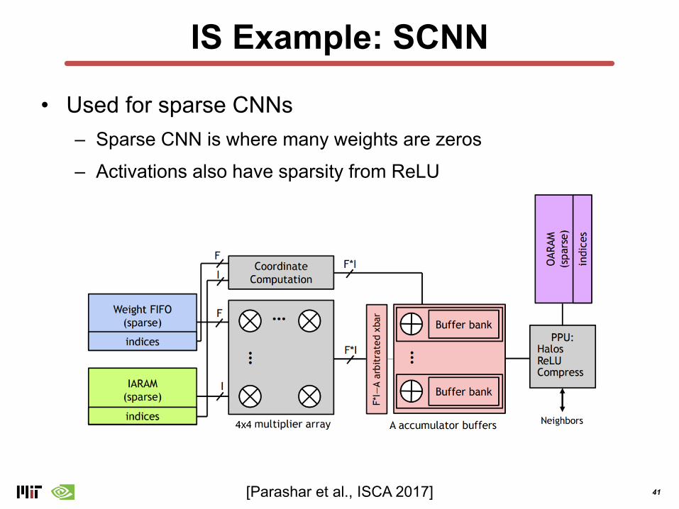
IS Example: SCNN
• Used for sparse CNNs– Sparse CNN is where many weights are zeros
– Activations also have sparsity from ReLU
[Parashar et al., ISCA 2017]
42
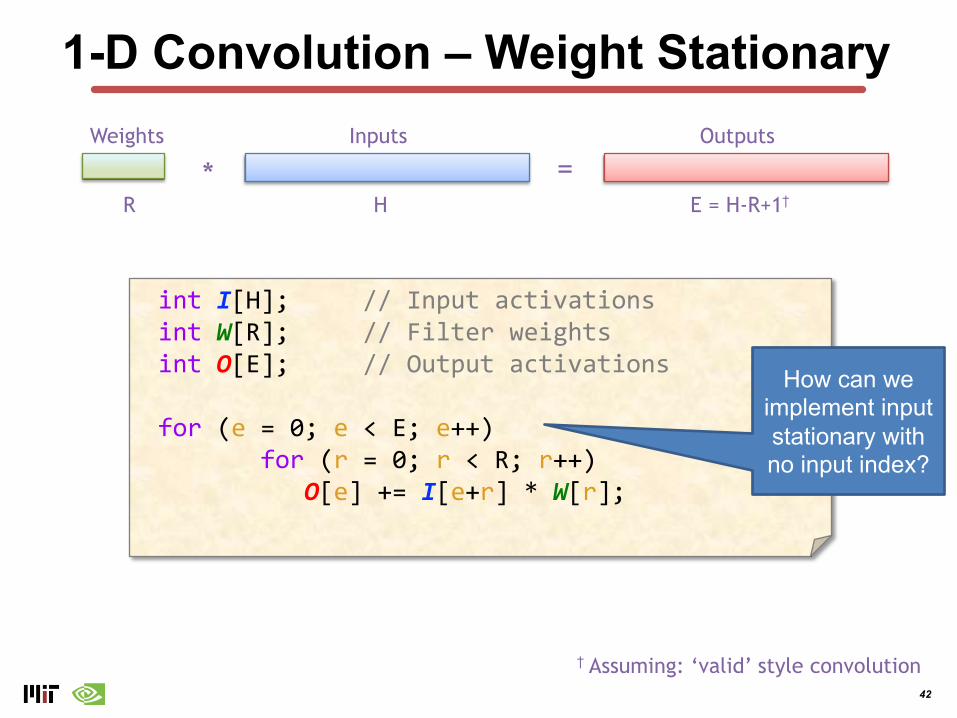
1-D Convolution – Weight Stationary
R
Weights
H
Inputs
E = H-R+1†
Outputs
* =
int I[H]; // Input activationsint W[R]; // Filter weightsint O[E]; // Output activations
for (e = 0; e < E; e++) for (r = 0; r < R; r++)
O[e] += I[e+r] * W[r];
† Assuming: ‘valid’ style convolution
How can we implement input stationary with no input index?

43
1-D Convolution – Input Stationary
R
Weights
H
Inputs
E = H-R+1†
Outputs
* =
int I[H]; // Input activationsint W[R]; // Filter weightsint O[E]; // Output activations
for (h = 0; h < H; h++) for (r = 0; r < R; r++)
O[h-r] += I[h] * W[r];
† Assuming: ‘valid’ style convolution
Beware w-r must be >= 0
and <E
44
Reference Patterns ofDifferent Dataflows
45
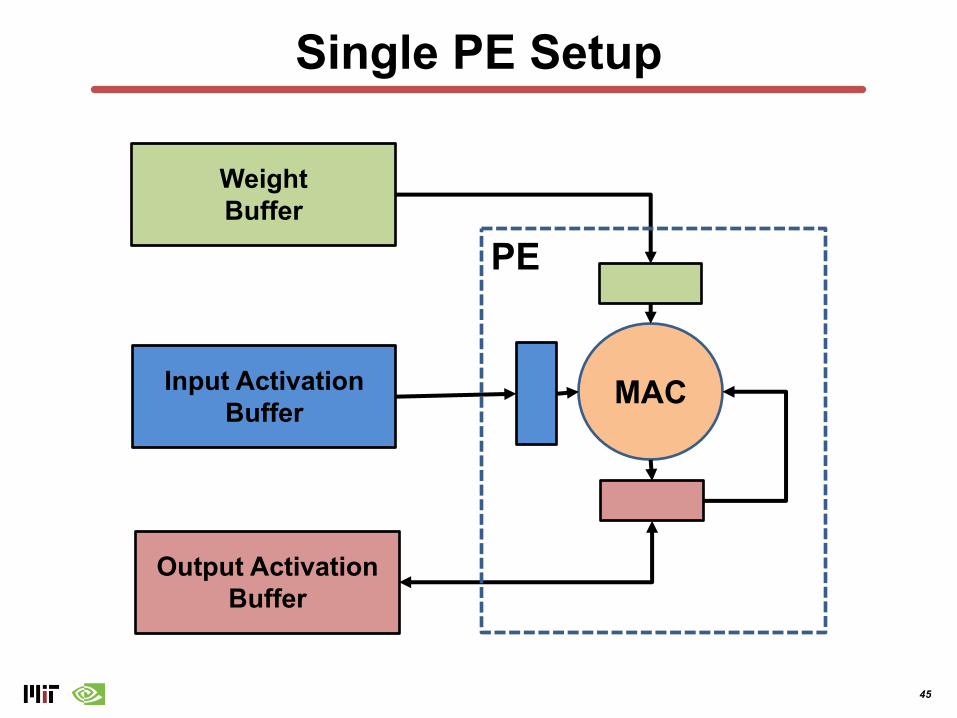
Single PE Setup
WeightBuffer
Input ActivationBuffer
Output ActivationBuffer
MAC
PE
46
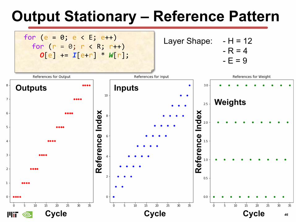
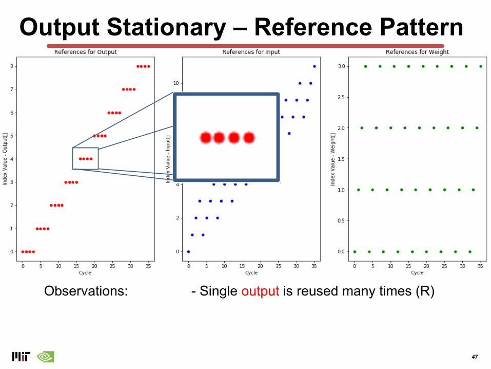
Output Stationary – Reference PatternLayer Shape: - H = 12
- R = 4- E = 9
for (e = 0; e < E; e++) for (r = 0; r < R; r++) O[e] += I[e+r] * W[r];
Cycle Cycle Cycle
Ref
eren
ce In
dex
Ref
eren
ce In
dex
Outputs InputsWeights
47
Output Stationary – Reference Pattern
Observations: - Single output is reused many times (R)
48
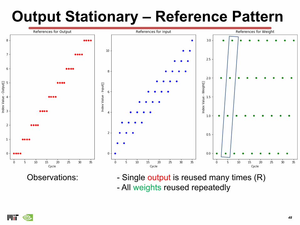
Output Stationary – Reference Pattern
Observations: - Single output is reused many times (R)- All weights reused repeatedly
49
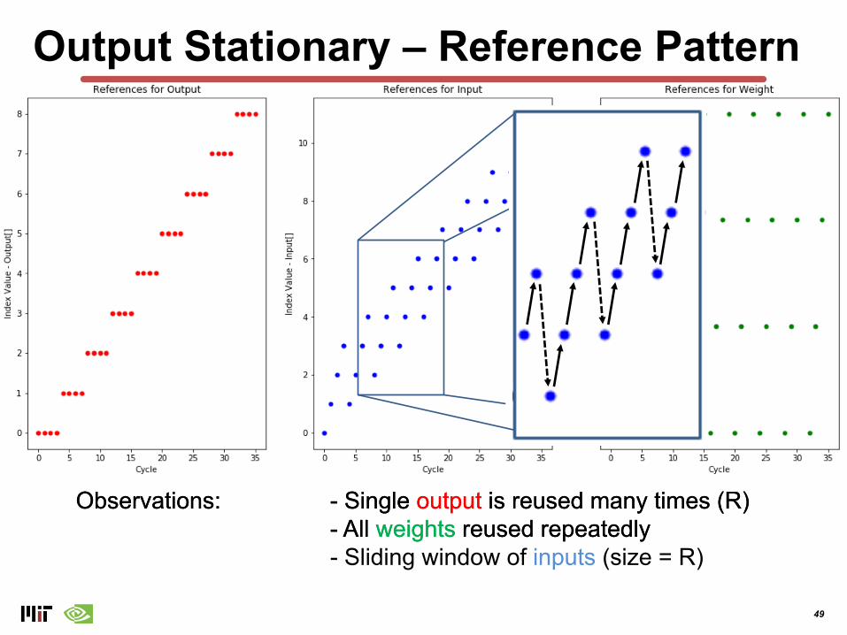
Output Stationary – Reference Pattern
Observations: - Single output is reused many times (R)- All weights reused repeatedly- Sliding window of inputs (size = R)
Observations: - Single output is reused many times (R)- All weights reused repeatedly
50
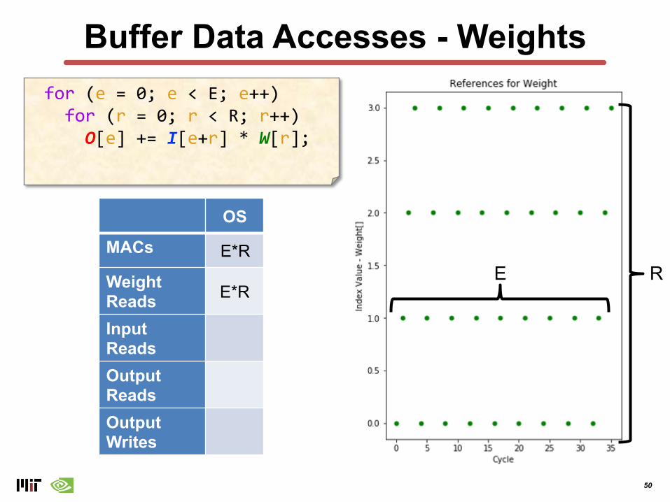
Buffer Data Accesses - Weightsfor (e = 0; e < E; e++) for (r = 0; r < R; r++)
O[e] += I[e+r] * W[r];
OS
MACs
Weight ReadsInput ReadsOutput ReadsOutput Writes
REE*R
E*R
51
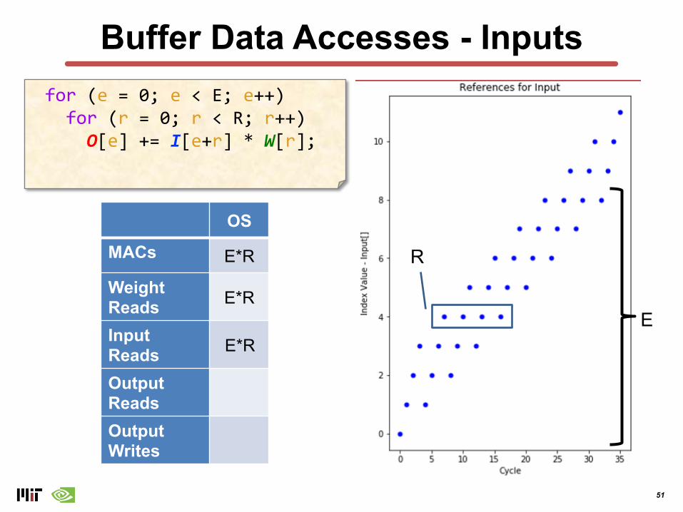
Buffer Data Accesses - Inputs
OS
MACs E*R
Weight Reads E*R
Input ReadsOutput ReadsOutput Writes
E
R
E*R
for (e = 0; e < E; e++) for (r = 0; r < R; r++)
O[e] += I[e+r] * W[r];
52
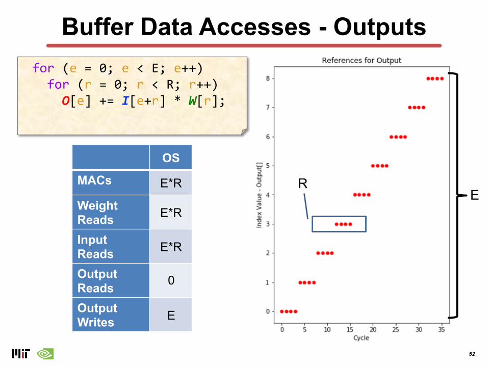
Buffer Data Accesses - Outputs
OS
MACs E*R
Weight Reads E*R
Input Reads E*R
Output ReadsOutput Writes
ER
0
E
for (e = 0; e < E; e++) for (r = 0; r < R; r++)
O[e] += I[e+r] * W[r];
53
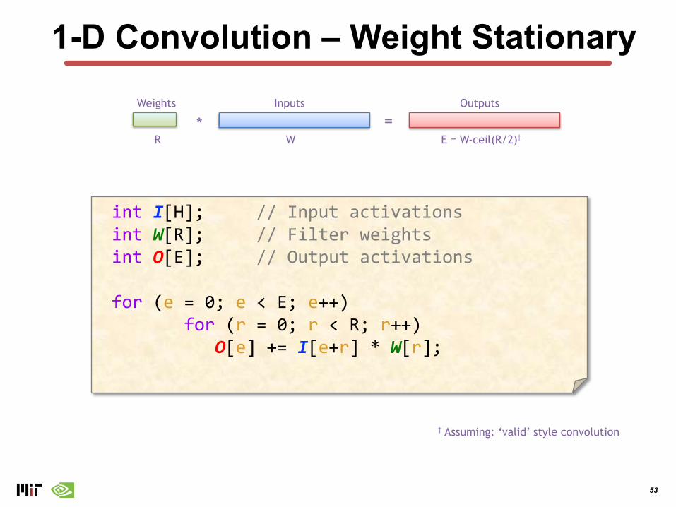
1-D Convolution – Weight Stationary
R
Weights
W
Inputs
E = W-ceil(R/2)†
Outputs
* =
† Assuming: ‘valid’ style convolution
int I[H]; // Input activationsint W[R]; // Filter weightsint O[E]; // Output activations
for (e = 0; e < E; e++) for (r = 0; r < R; r++)
O[e] += I[e+r] * W[r];
54
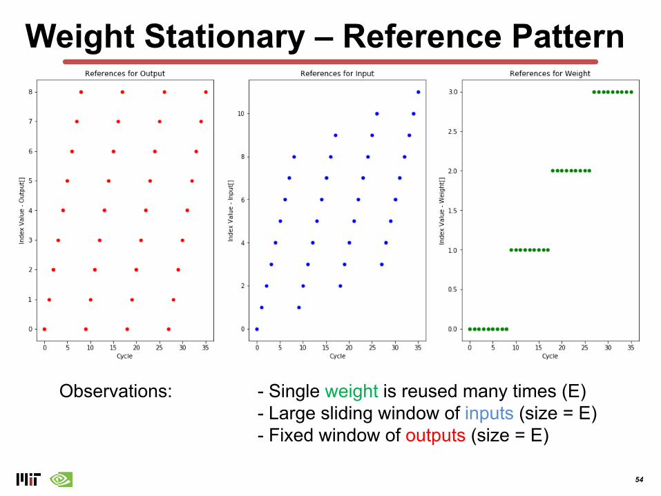
Weight Stationary – Reference Pattern
Observations: - Single weight is reused many times (E)- Large sliding window of inputs (size = E)- Fixed window of outputs (size = E)
55
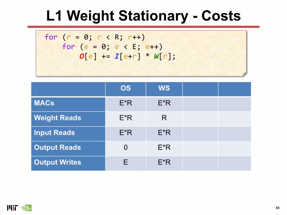
L1 Weight Stationary - Costsfor (r = 0; r < R; r++)
for (e = 0; e < E; e++)O[e] += I[e+r] * W[r];
OS WS
MACs E*R E*R
Weight Reads E*R R
Input Reads E*R E*R
Output Reads 0 E*R
Output Writes E E*R
56
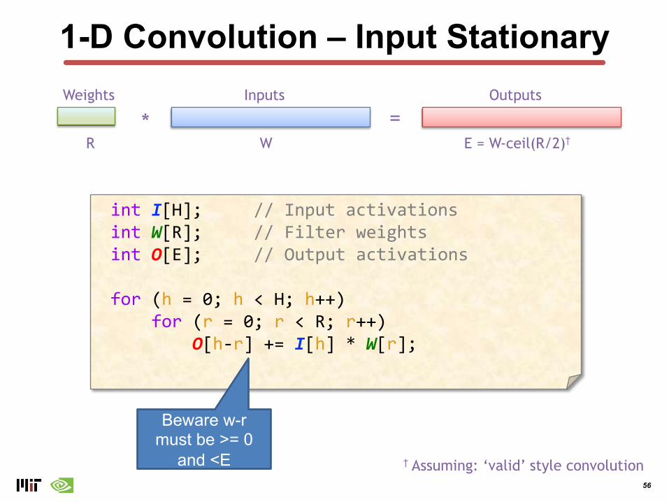
1-D Convolution – Input Stationary
R
Weights
W
Inputs
E = W-ceil(R/2)†
Outputs
* =
† Assuming: ‘valid’ style convolution
int I[H]; // Input activationsint W[R]; // Filter weightsint O[E]; // Output activations
for (h = 0; h < H; h++) for (r = 0; r < R; r++)
O[h-r] += I[h] * W[r];
Beware w-r must be >= 0
and <E
57
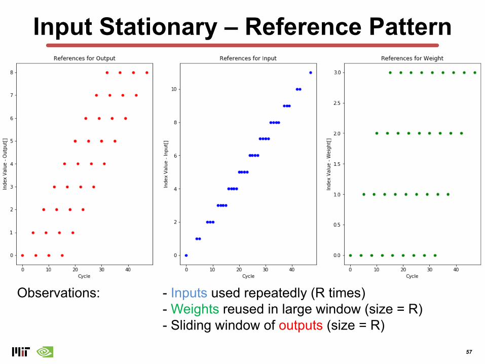
Input Stationary – Reference Pattern
Observations: - Inputs used repeatedly (R times)- Weights reused in large window (size = R)- Sliding window of outputs (size = R)
58
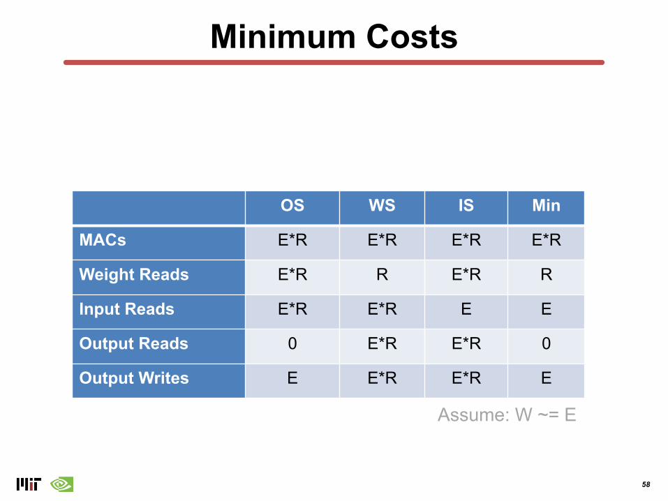
Minimum Costs
OS WS IS Min
MACs E*R E*R E*R E*R
Weight Reads E*R R E*R R
Input Reads E*R E*R E E
Output Reads 0 E*R E*R 0
Output Writes E E*R E*R E
Assume: W ~= E
59
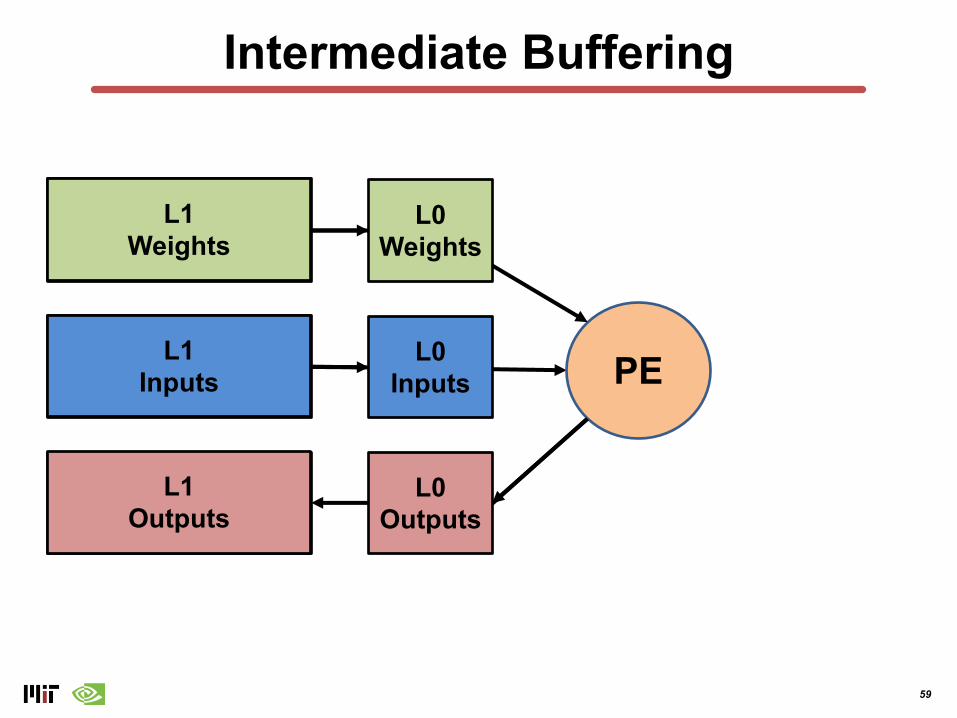
Intermediate Buffering
L0Weights
L0Inputs
L0Outputs
PE
L0Weights
L0Inputs
L0 Outputs
L1Weights
L1Inputs
L1Outputs
60
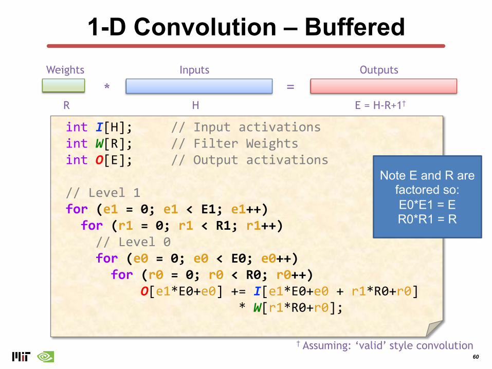
1-D Convolution – Buffered
R
Weights
H
Inputs
E = H-R+1†
Outputs
* =
int I[H]; // Input activationsint W[R]; // Filter Weightsint O[E]; // Output activations
// Level 1for (e1 = 0; e1 < E1; e1++) for (r1 = 0; r1 < R1; r1++)
// Level 0for (e0 = 0; e0 < E0; e0++) for (r0 = 0; r0 < R0; r0++)
O[e1*E0+e0] += I[e1*E0+e0 + r1*R0+r0]* W[r1*R0+r0];
† Assuming: ‘valid’ style convolution
Note E and R are factored so:E0*E1 = ER0*R1 = R
61
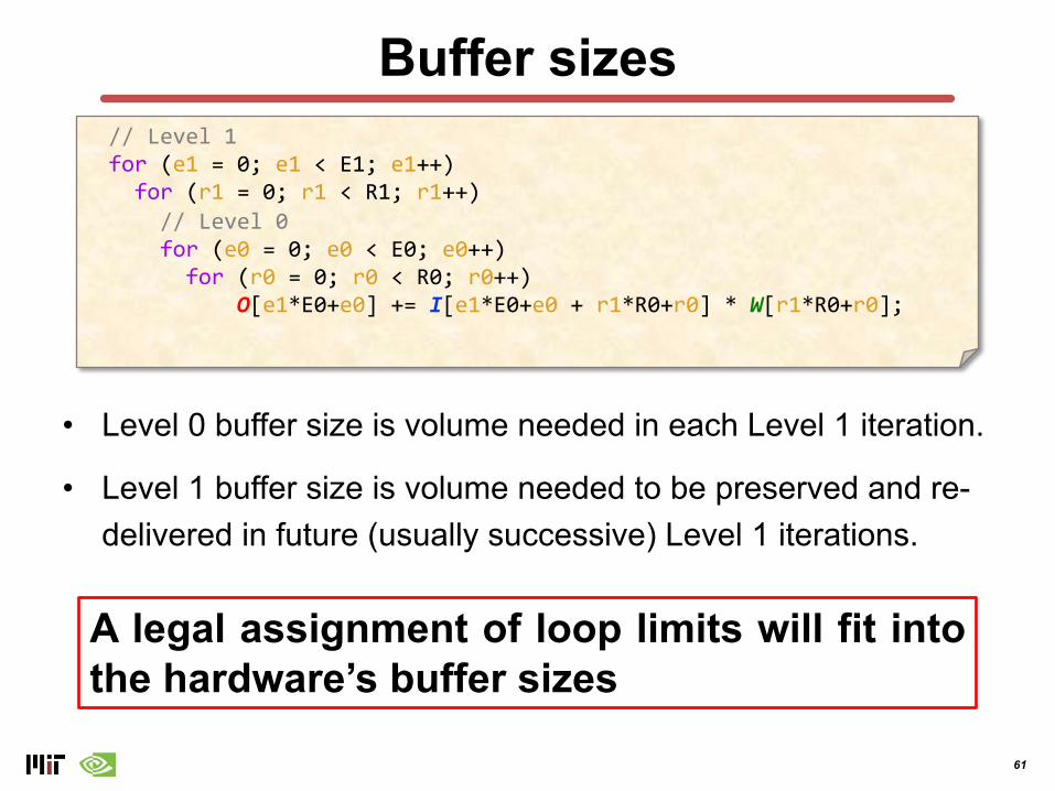
Buffer sizes
• Level 0 buffer size is volume needed in each Level 1 iteration.
• Level 1 buffer size is volume needed to be preserved and re-delivered in future (usually successive) Level 1 iterations.
// Level 1for (e1 = 0; e1 < E1; e1++) for (r1 = 0; r1 < R1; r1++)// Level 0for (e0 = 0; e0 < E0; e0++) for (r0 = 0; r0 < R0; r0++)
O[e1*E0+e0] += I[e1*E0+e0 + r1*R0+r0] * W[r1*R0+r0];
A legal assignment of loop limits will fit intothe hardware’s buffer sizes
62
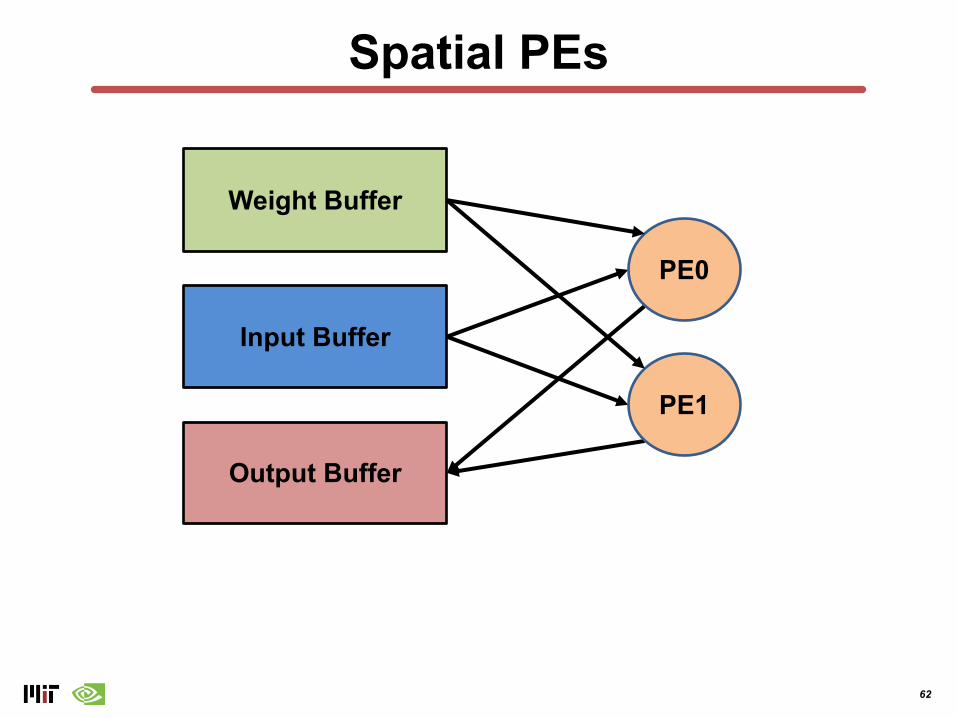
Spatial PEs
Weight Buffer
Input Buffer
Output Buffer
PE0
PE1
63
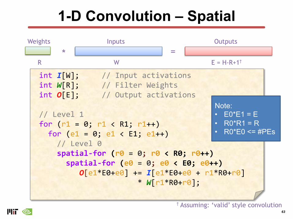
1-D Convolution – Spatial
R
Weights
W
Inputs
E = H-R+1†
Outputs
* =
int I[W]; // Input activationsint W[R]; // Filter Weightsint O[E]; // Output activations
// Level 1for (r1 = 0; r1 < R1; r1++)for (e1 = 0; e1 < E1; e1++)
// Level 0spatial-for (r0 = 0; r0 < R0; r0++)spatial-for (e0 = 0; e0 < E0; e0++)
O[e1*E0+e0] += I[e1*E0+e0 + r1*R0+r0]* W[r1*R0+r0];
† Assuming: ‘valid’ style convolution
Note:• E0*E1 = E• R0*R1 = R• R0*E0 <= #PEs
64
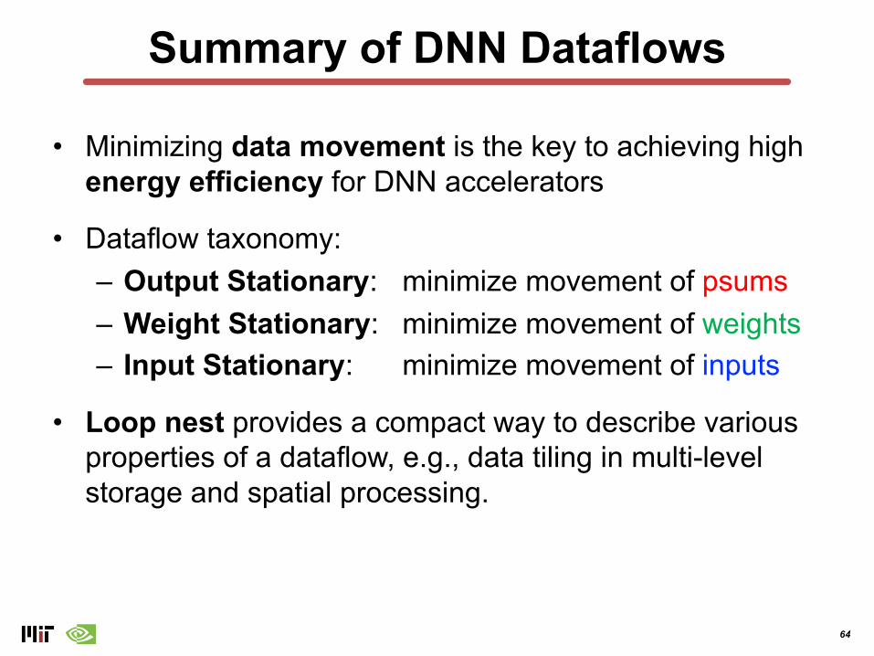
Summary of DNN Dataflows
• Minimizing data movement is the key to achieving high energy efficiency for DNN accelerators
• Dataflow taxonomy:– Output Stationary: minimize movement of psums– Weight Stationary: minimize movement of weights– Input Stationary: minimize movement of inputs
• Loop nest provides a compact way to describe various properties of a dataflow, e.g., data tiling in multi-level storage and spatial processing.