Am. ]. Hum. Genet. 46:358-368, 1990

DNA Fingerprinting for Forensic Identification: Potential Effects on Data Interpretation of Subpopulation Heterogeneity and Band Number Variability

Joel E. Cohen

Rockefeller University, New York

Summary

Some methods of statistical analysis of data on DNA fingerprinting suffer serious weaknesses. Unlinked Mendelizing loci that are at linkage equilibrium in subpopulations may be statistically associated, not statistically independent, in the population as a whole if there is heterogeneity in gene frequencies between subpopulations. In the populations where DNA fingerprinting is used for forensic applications, the as­sumption that DNA fragments occur statistically independently for different probes, different loci, or differ­ent fragment size classes lacks supporting data so far; there is some contrary evidence. Statistical associa­tion of alleles may cause estimates based on the assumption of statistical independence to understate the true matching probabilities by many orders of magnitude. The assumptions that DNA fragments occur in­dependently and with constant frequency within a size class appear to be contradicted by the available data on the mean and variance of the number of fragments per person. The mistaken use of the geometric mean instead of the arithmetic mean to compute the probability that every DNA fragment of a randomly chosen person is present among the DNA fragments of a specimen may substantially understate the proba­bility of a match between blots, even if other assumptions involved in the calculations are taken as correct. The conclusion is that some astronomically small probabilities of matching by chance, which have been claimed in forensic applications of DNA fingerprinting, presently lack substantial empirical and theoretical support.

Introduction

Minisatellites are regions of the genome in which a DNA sequence is repeated tandemly for a variable number of times. Minisatellites are dispersed in the genomes of humans and other mammals. A subset of the repeated DNA sequences contains a short, shared "core" sequence (Jeffreys et al. 1985a). Different subsets of minisatel­lites share different core sequences. Minisatellites that contain a given core sequence can be detected by a hy­bridization probe that consists of the core sequence repeated in tandem.

Received July 17, 1989; revision received September 18, 1989. Address for correspondence and reprints: Until June 3, 1990-

Joel E. Cohen, Institute for Advanced Study, Olden Lane, Princeton, NJ 08540; after June 3, 1990-Joel E. Cohen, Rockefeller Univer­sity, 1230 York Avenue, Box 20, New York, NY 10021-6399. © 1990 by The American Society of Human Genetics. All rights reserved. 0002-9297/90/4602-0016$02.00

358

When human DNA is digested by a restriction t'n­zyme and hybridized with a specific core probe, the resulting fragments can be distributed according to size by a Southern blot. This procedure reveals the sizes of fragments that contain a specific core. The pattern of fragment sizes is highly variable or polymorphic from one individual to another (except for identical twins) but is apparently highly stable or conserved both from one tissue to another and over time within a given in­dividual (Jeffreys et al. 1985a ). The combination of vari­ability among individuals and stability within an in­dividual suggests that the patterns of fragment sizes revealed by specific probes might serve as useful in­dividual identifiers, or "DNA fingerprints" (Jeffreys et al. 1985b).

In forensic practice, the patterns of DNA fragment sizes are usually determined by one of two distinct proce­dures. One procedure, common in the United States,

DNA Fingerprinting

uses several single-locus probes serially. The other pro­cedure, common in the United Kingdom, uses a single probe that detects alleles at multiple loci.

In forensic applications of DNA fingerprints, a spec­imen's pattern of DNA fragment sizes is compared with a collection of such patterns from some set of people. A measure of similarity between any two such patterns is defined. Then a probability of observing, by chance alone, a given level of similarity is computed. If the spec­imen's pattern has a priori a very low chance of being similar to the pattern of a randomly chosen person, and if, nevertheless, the specimen's pattern is observed to be very similar to the pattern of some particular per­son, then it is concluded that the individual whose pat­tern matches that of the specimen is the source of the specimen, with high probability.

The scope of the present paper is limited to statisti­cal problems in the analysis of data on matches between DNA fragments of various sizes for the purpose of iden­tifying an individual by means of a specimen. Some published procedures appear to lack adequate empiri­cal or theoretical support. The following sections ad­dress problems raised by (1) heterogeneity in popula­tions, ( 2) calculating the probability that a given match between two fingerprints would arise at random, and ( 3) calculating the average power of a fingerprint. As the present paper is intended to be constructive as well as critical, some procedures, experiments, and analy­ses are suggested which could provide a firmer founda­tion for the use of DNA fingerprinting for forensic identification.

The present paper does not deal with uncertainties and ambiguities in the underlying biochemical proce­dures and data, such as the problems of collecting un­contaminated specimens at the scene of a crime, degra­dation of materials prior to analysis, use of internal controls and mixture experiments in electrophoretic gels, the necessity for "blind" judgments and probabilis­tic assessment of a match between bands in different lanes of a gel or on different gels, and others (e.g., see Lander 1989; Lewin 1989; Sensabaugh and Witkowski 1989). The present paper does not deal with questions of laboratory protocol, such as the chain of custody of samples and quality assurance (Sensabaugh and Wit­kowski 1989). Although recent journalistic accounts suggest that routine laboratory error rates for this kind of test may be as high as 1%-5% (according to a ref­eree), procedures for reducing these error rates are in principle well understood and could be applied in sen­sitive cases. The present paper does not deal with legal questions, such as the admissibility or presentation of

359

DNA fingerprinting data in court or pretrial hearings and the determination of a quantitative threshold for a probability that is "beyond a reasonable doubt" (e.g., see Tribe 1971; Fienberg and Schervish 1986). The pres­ent paper does not deal in detail with the use of DNA fingerprinting to establish genetic relationships among people-e.g., in paternity testing-although it will be apparent that many of the problems discussed below arise also in paternity testing. In genealogical applica­tions, a high spontaneous mutation rate to minisatel­lites of different lengths has been noted (Jeffreys et al. 1988).

Population Heterogeneity and Statistical Dependence of Alleles

The methods that have been used to infer probabili­ties of identification by using DNA fingerprinting ap­pear to overlook population heterogeneity in gene fre­quencies. A simplified example will show that such heterogeneity may render invalid a key assumption made in applications of DNA fingerprinting. This example contains no new genetics or statistics, but the issues it raises have not received adequate attention. These issues apply equally to fingerprinting procedures based on single-locus probes and to those based on multi­locus probes.

Consider a large human population (e.g., Britain) in which one probe detects allelic variation in restriction­fragment length at one autosomal locus and in which another probe detects allelic variation in restriction­fragment length at another autosomal locus. Suppose there are just two alleles at each locus. Call the alleles at the first locus A and a, and call the alleles at the second locus Band b. No dominance between alleles is implied: A, a, B, and beach are assumed to correspond to well-defined distinct bands, so that the genotype of an individual (at these two loci) can be unequivocally determined from inspection of a gel. Suppose also that the two loci are located either on different autosomes or far enough apart on the same autosome so that the recombination fraction between loci is 112. Suppose also that inheritance at each locus is strictly Mendelian. So far this is a textbook model of two loci with two alleles (e.g., see Crow and Kimura 1970).

Now suppose that Britain contains two subpopula­tions. Call the two subpopulations F and G. Suppose that within each subpopulation the two loci are in link­age equilibrium and that there is random mating and no selection with respect to both loci. Let p(A,F) de­note the gene frequency of allele A in subpopulation

360

F. More generally, let p(i, H) denote the gene frequency of allele i in subpopulation H, where i = A, a, B, b and H = E, F. Thus p(A, F) + p(a, F) = 1, P(B, F) + p(b, F) = 1, and similarly with F replaced by G.

Under the preceding assumptions, within each sub­population each band (allele) is statistically indepen­dent: the genotype frequencies within a subpopulation are simply the products of the appropriate gene frequen­cies within that subpopulation. For example, if .f{AABb, F) denotes the relative frequency of the AA homozygote at the first locus and of the Bb heterozygote at the sec­ond locus in subpopulation F, then.f{AABb, F) = p(A, F)lp(B, F)p(b, F).

If the gene frequencies are different in the two sub­populations, it is not in general true that each band (allele) is statistically independent in the population as a whole. On the contrary, in the population, different bands may be positively or negatively associated, de­pending on the proportions of people in the different subpopulations and on the differences of the allele fre­quencies at each locus. Statisticians have known for a long time (Yule 1903) that attributes (allele frequen­cies, in this case) may be positively or negatively as­sociated in a population as a result of pooling the fre­quency of the attributes in subpopulations in which the attributes are independent. This phenomenon, still of active interest (Good and Mittal1987), appears to have been overlooked in forensic applications of DNA fingerprinting.

A numerical example, using completely arbitrary figures, illustrates the phenomenon. Suppose the frac­tions of the whole population that belong to subpopu­lations F and G are given by n(F) = .9 and n(G) = .1. Suppose that p(A, F) = .3, p(A, G) = .6, p(B, F) = .4, and p(B, G) = .8. The overall relative frequency of the A allele in the population is p(A) = p(A, F)n(F) + p(A, G)n(G) = .33, whence p(a) = 1 - p(A) = .67 is the overall relative frequency of the a allele. Simi­larly, p(B) = .44 and p(b) = 1 - p(B) = .56. The actual relative frequency of the AABB genotype in the population is.f{AABB) = p(A, F)2p(B, f)ln(F) + p(A, G)lp(B, G)2n(G) = .036. However, if the relative fre­quency of the AABB genotype in the population is cal­culated assuming independence between alleles (bands), the estimate is j""(AABB) = p(A)2p(B)2 = .021.

To make the example slightly more realistic, assume that, within each subpopulation, the alleles At, Az, ... , Ato have the same allele frequency as A (so that at, az, ... , ato have the same allele frequency as a) and that the alleles Bt, Bz, . . . , Bto have the same allele frequency as B (so that bt, bz, ... , bto have

Cohen

the same allele frequency as b) and that the different alleles are statistically independent. The actual relative frequency of the homozygous genotype AtAtAzAz ... AtoAtoBtBtBzBz ... BtoBto in the whole population is [p(A, F)2p(B, F)2]1°n(F) + [p(A, G)2p(B, G)2]1° n(G) = 4.2 x 10-s. However, if the relative frequency of the genotype in the population is calculated assuming independence between alleles (bands), the estimated rel­ative frequency of the homozygous genotype AtAtAzAz ... AtoAtoBtBtBzBz ... BtoBto is [p(A)2p(B)2JIO = 1.7 x t0- 17• Now suppose a forensic specimen is de­termined to have the homozygous genotype AtAtAzAz ... AtoAtoBtBtBzBz ... BtoBto by DNA fingerprint­ing, and suppose a suspect individual is identified whose genotype exactly matches that of the specimen. In this case, the estimated probability of a match, when inde­pendence of alleles is assumed, is lower than the true probability of a match when one allows for the hetero­geneity of subpopulations, by a factor of more than 10-9• The estimated probability, being lower than the true probability, exaggerates the significance of a match and unnecessarily incriminates the suspect. The numer­ical values in this example were chosen in advance for simplicity, rather than being selected to illustrate a worst case.

This hypothetical example resembles reality in that there is likely to be significant genetic heterogeneity in real populations. The allele frequencies of genes of med­ical interest differ from one human subpopulation to another. Minisatellite regions and other RFLPs that serve as markers of disease-related genes (Gusella et al. 1983; Jeffreys et al. 1986) are likely to share that heterogeneity. The DNA probes used for forensic iden­tification detect alleles that have heterogeneous allele frequencies: Lander (1989, p. 504), using Wahlund's formula, found excess homozygosity (relative to Hardy­Weinberg equilibrium) at loci identified by DNA probes in the Hispanic population used as the reference popu­lation in a murder trial, demonstrating "the presence of genetically distinct subgroups within the Hispanic sample."

The hypothetical example given above differs from reality in that neither the assumption of just two sub­populations nor the particular allele frequencies and subpopulation frequencies assumed are likely to be realistic. The actual effect of subpopulation heteroge­neity could be larger or smaller than that in this example.

The example demonstrates three points. First, the population used to obtain estimates of allele frequen­cies is crucial for subsequent applications of match prob­abilities to individual cases. Future studies should care-

DNA Fingerprinting

fully define a reference population (what statisticians call a sampling universe) which is to be studied, and they should make explicit the procedure (such as sys­tematic sampling or random sampling) that is used to sample from this population. Options and procedures for proper sampling have been clearly described else­where (e.g., see Snedecor and Cochran 1980, chap. 21).

There are good practical and scientific reasons for giving serious attention to sampling. In practice, if a study that attempts to derive matching probabilities for DNA fingerprinting is based on an ill-specified sample, the resulting probabilities can be challenged in court on the grounds that the study sample is not the sample most appropriate to the accused individual. If the propo­nents of DNA fingerprinting wish to claim that the prob­abilities of matching at random are astronomically low for virtually all populations, they are obliged to dem­onstrate the claim for at least several well-defined popu­lations. Scientifically, DNA fingerprinting provides a means of assessing the genetic heterogeneity of popu­lations. Studies of well-defined samples offer an oppor­tunity to compare the genetic variability of different populations and could be of potential interest to stu­dents of human evolution (Lander 1989, p. 504).

Second, alleles (bands) may be significantly statisti­cally associated in a population if there is heterogene­ity between subpopulations in the allele frequencies, even though the loci involved may be strictly Mendelian, unlinked, and at linkage equilibrium within each sub­population. Wherever subpopulations are heteroge­neous, true random samples of populations are required to measure directly whether any statistical association of minisatellite alleles results from pooling across sub­populations.

Third, the statistical association of alleles, though undetectable either in terms of chromosomal mecha­nisms or within homogeneous subpopulations, may in­duce significant errors in estimates of match probabili­ties if the estimates ignore the statistical association.

Among statisticians, the gratuitous assumption of in­dependence is well known as a source of superficially persuasive arguments for the existence of miracles (Kru­skal1988), which correspond in the present situation to extravagantly small alleged probabilities of obtain­ing a match at random.

Calculating the Probability of a Match at Random

Given a match between the DNA fingerprint of a spec­imen and the DNA fingerprint of an individual, how

361

can one calculate the probability that this match could have arisen at random? An obvious possibility is to rec­ord the complete genetic pattern (not broken into dis­crete bands) of each individual in a population survey and then count how many complete patterns match that of the specimen. If S individuals are surveyed, this ap­proach cannot yield a probability of match lower than liS (given that one individual's pattern matches the spec­imen's pattern). To obtain, by this approach, the ex­tremely low probabilities of a match quoted in many forensic applications of DNA fingerprinting would re­quire surveying more people than are alive. Since this would be difficult, the quoted low probabilities are ob­tained from calculations based on simplifying assump­tions about the occurrence of bands in different regions of Southern blots. The results of the calculations may be in error if the assumptions are not justified.

Among the major assumptions sometimes made are the following:

1. The probability of a match for a given probe and fragment size class has been estimated by random sampling of a well-defined, genetically homogeneous reference population.

2. Matching of DNA fragments identified with one probe or at one genetic locus is independent of match­ing fragments identified with any other probe or at any other genetically unlinked locus.

3. For a given probe, the fragments identified may be categorized into size classes, and matching of DNA fragments in one size class is independent of match­ing in any other size class.

4. Within a size class of DNA fragments identified by a given probe, the probability of a match is constant for all fragments in the size class, and matching is independent for any two different fragments within the class, and there is no variability in the number of fragments per specimen or per person in the size class.

There is considerable evidence against these assump­tions in some applications of DNA fingerprinting.

Regarding the first assumption, Jeffreys et al. (1985b) report data based on "a random sample of 20 unrelated British caucasians" who were, in fact, "20 volunteer white students from our university [University of Lei­cester]" (A. J. Jeffreys, personal communication, Au­gust 28, 1988). Similarly, Gill et al. (1987) analyze, among other materials, whole blood samples from 41 individuals of unspecified origin and characteristics. Such subjects do not represent a genuine random sam­ple, in the technical sense (Snedecor and Cochran 1980,

362

chap. 21), of the entire "British caucasian" population. Such a sample requires a list or sampling frame from which a sample is randomly selected. The special popu­lation from which the subjects were drawn should be remembered before using the data for inferences about any other population.

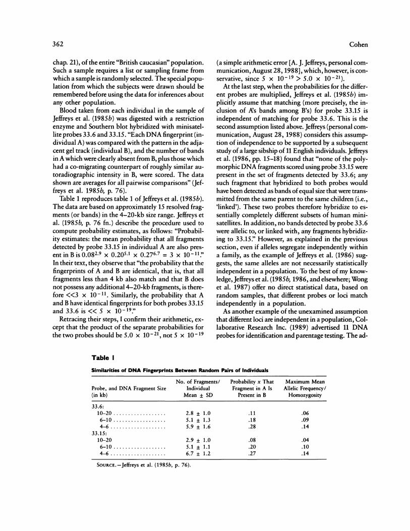
Blood taken from each individual in the sample of Jeffreys et al. (1985b) was digested with a restriction enzyme and Southern blot hybridized with minisatel­lite probes 33.6 and 33.15. "Each DNA fingerprint (in­dividual A) was compared with the pattern in the adja­cent gel track (individual B), and the number of bands in A which were dearly absent from B, plus those which had a co-migrating counterpart of roughly similar au­toradiographic intensity in B, were scored. The data shown are averages for all pairwise comparisons" (Jef­freys et al. 1985b, p. 76).

Table 1 reproduces table 1 of Jeffreys et al. (1985 b). The data are based on approximately 15 resolved frag­ments (or bands) in the 4-20-kb size range. Jeffreys et al. (1985b, p. 76 fn.) describe the procedure used to compute probability estimates, as follows: "Probabil­ity estimates: the mean probability that all fragments detected by probe 33.15 in individual A are also pres­ent in B is 0.082.9 x 0.205·1 x 0.276·7 = 3 x 10-11 :• In their text, they observe that "the probability that the fingerprints of A and B are identical, that is, that all fragments less than 4 kb also match and that B does not possess any additional4-20-kb fragments, is there­fore < <3 x 10 - 11 . Similarly, the probability that A and B have identical fingerprints for both probes 33.15 and 33.6 is<< 5 x lQ-19."

Retracing their steps, I confirm their arithmetic, ex­cept that the product of the separate probabilities for thetwoprobesshouldbe5.0 x 10-21,not5 x lQ-19

Table I

Cohen

(a simple arithmetic error [A. J. Jeffreys, personal com­munication, August 28, 1988], which, however, is con­servative, since 5 x 10-19 > 5.0 x 10-21).

At the last step, when the probabilities for the differ­ent probes are multiplied, Jeffreys et al. (1985b) im­plicitly assume that matching (more precisely, the in­clusion of Xs bands among B's) for probe 33.15 is independent of matching for probe 33.6. This is the second assumption listed above. Jeffreys (personal com­munication, August 28, 1988) considers this assump­tion of independence to be supported by a subsequent study of a large sibship of 11 English individuals. Jeffreys et al. (1986, pp. 15-18) found that "none of the poly­morphic DNA fragments scored using probe 33.15 were present in the set of fragments detected by 33.6; any such fragment that hybridized to both probes would have been detected as bands of equal size that were trans­mitted from the same parent to the same children (i.e., 'linked'). These two probes therefore hybridize to es­sentially completely different subsets of human mini­satellites. In addition, no bands detected by probe 33.6 were allelic to, or linked with, any fragments hybridiz­ing to 33.15:' However, as explained in the previous section, even if alleles segregate independently within a family, as the example of Jeffreys et al. (1986) sug­gests, the same alleles are not necessarily statistically independent in a population. To the best of my know­ledge, Jeffreys et al. (1985b, 1986, and elsewhere; Wong et al. 1987) offer no direct statistical data, based on random samples, that different probes or loci match independently in a population.

As another example of the unexamined assumption that different loci are independent in a population, Col­laborative Research Inc. (1989) advertised 11 DNA probes for identification and parentage testing. The ad-

Similarities of DNA Fingerprints Between Random Pairs of Individuals

Probe, and DNA Fragment Size (in kb)

33.6: 10-20 ................. . 6-10 ................. . 4-6 .................. .

33.15: 10-20 6-10 ................. . 4-6 .................. .

No. of Fragments/ Individual

Mean± SD

2.8 ± 1.0 5.1 ± 1.3 5.9 ± 1.6

2.9 ± 1.0 5.1 ± 1.1 6.7 ± 1.2

SOURCE.-Jeffreys et al. (1985b, p. 76).

Probability x That Fragment in A Is

Present in B

.11

.18

.28

.08

.20

.27

Maximum Mean Allelic Frequency I

Homozygosity

.06

.09

.14

.04

.10

.14

DNA Fingerprinting

vertisement listed a "probability of identity" for each probe, followed by a "probability of identity" for "all loci combined" of 4. 96 x 10- 15• According to Stan­ley D. Rose, Director of DNA Products and Services for Collaborative Research Inc. (personal communica­tion, July 18, 1989 ), two of the probes recognize differ­ent polymorphisms at the same locus; one of these probes was excluded in calculating the probability of identity for all loci combined. After that exclusion, ac­cording to Rose, "the cumulative average probability of identity is based on the assumption that all loci seg­regate independently:• Rose notes that, "although these probes provide an extremely powerful tool for identifica­tion of individuals, it should be pointed out that we (collectively speaking) know relatively little about the characteristics of DNA polymorphisms in large popu­lations, or how the frequency distributions of specific alleles may differ in sub-populations:'

At the penultimate step of their calculation, when the match probabilities for different size classes of frag­ments (identified by a single probe) are being multi­plied, Jeffreys et al. (1985 b) implicitly assume that there is no statistical association between any two minisatel­lite regions in different size classes, so that matching in one size class of fragments is statistically indepen­dent of matching in any other size class. This is the third assumption listed above.

Later evidence argues against the assumption of statistical independence among fragments. One dog family displayed dear associations {positive and nega­tive) among fragments of different lengths generated by DNA fingerprinting (Jeffreys and Morton 1987, pp. 8, 11). A large sibship of English humans displayed sev­eral allelic pairs of both paternal and maternal frag­ments identified by both probes; there was a linked pair of fragments in this and another pedigree (Jeffreys et al. 1986, p. 15). Moreover, alleles at the same locus span different categories of fragment length: "large differences in minisatellite allele lengths must exist, aris­ing presumably by unequal exchange in these tandem repetitive regions; several allelic pairs identified ... do indeed show substantial length differences" (Jeffreys et al. 1986, p. 18). These examples of statistical associa­tion (allelism or linkage) of fragments in different length categories within families could be amplified at the population level, as mentioned above, by heterogeneity among subpopulations.

At the first step of their calculation, in computing the match probability for DNA fragments within each size class (identified by a single probe), Jeffreys et al. (1985b) implicitly make three major approximations

363

(as in the fourth assumption listed above): (1) that the probability (denoted by x in table 1) that a fragment in A is also present in B is the same for all fragments in the size class, (2) that different fragments within a size class match or fail to match independently, and (3) that there is no variability in the number of frag­ments, either per specimen or per person, in the size class. Under these assumptions, it is correct to com­pute the probability of a match as Jeffreys et al. (1985 b) have done: if x is the probability that a fragment in A is present in B, and if n is the {putatively constant) number of fragments per person in the size class, then the probability that all the fragments in A in the given size class are also present in B is precisely xn.

In the remainder of this section, I examine the first two approximations: constancy of match probabilities within a size class and independence of matching. The third approximation, constancy in the number of frag­ments in the size class per specimen or per person, will be examined in the following section, because it relates to the major issue of calculating the average power of a match.

The assumption that the match probabilities are con­stant within a size class seems implausible, given the data in table 1, because the fragment match probability rises as the DNA fragment size falls, for both probes. It seems unlikely that the match probabilities change abruptly by discrete steps, precisely at the boundaries of the arbitrarily selected fragment-size classes. More likely, the match probabilities rise smoothly with fall­ing fragment size. However, using a fixed average x is a conservative approximation, in that it overstates the probability of a match (as may easily be shown by con­structing a numerical example). Reanalysis of the raw data on which table 1 is based, by using finer size cate­gories, or analysis of more extensive other data, could show whether the match probabilities are indeed con­stant within the given size classes.

Gillet al. (1987, table 2) also assume a constant prob­ability of matching for fragments of different sizes in their analysis of the frequency distribution of the num­ber of matches between individuals. They use two mea­sures of matching: inclusion of the bands of individual A among those of individual B (like Jeffreys et al. [1985 b]) and identity between the bands of individuals A and B (equivalent to inclusion in both directions). They use the binomial distribution to compute the prob­ability of each possible number of matches under each definition of matching, and they find a reasonable agree­ment with the observed frequency distribution of num­ber of matches. This calculation assumes explicitly that

364

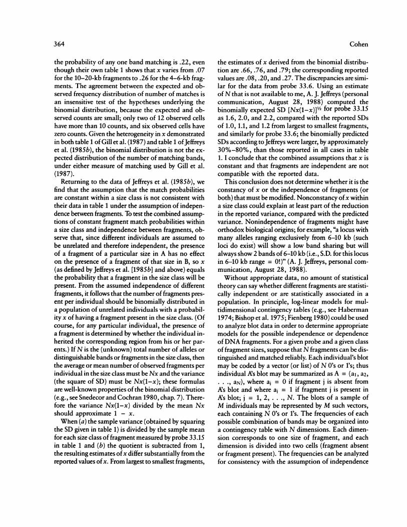
the probability of any one band matching is .22, even though their own table 1 shows that x varies from .07 for the 10-20-kb fragments to .26 for the 4-6-kb frag­ments. The agreement between the expected and ob­served frequency distribution of number of matches is an insensitive test of the hypotheses underlying the binomial distribution, because the expected and ob­served counts are small; only two of 12 observed cells have more than 10 counts, and six observed cells have zero counts. Given the heterogeneity in x demonstrated in both table 1 of Gillet al. (1987) and table 1 of Jeffreys et al. (1985b), the binomial distribution is not the ex­pected distribution of the number of matching bands, under either measure of matching used by Gill et al. (1987).

Returning to the data of Jeffreys et al. (1985b), we find that the assumption that the match probabilities are constant within a size class is not consistent with their data in table 1 under the assumption of indepen­dence between fragments. To test the combined ~ssump­tions of constant fragment match probabilities within a size class and independence between fragments, ob­serve that, since different individuals are assumed to be unrelated and therefore independent, the presence of a fragment of a particular size in A has no effect on the presence of a fragment of that size in B, so x (as defined by Jeffreys et al. [1985b] and above) equals the probability that a fragment in the size class will be present. From the assumed independence of different fragments, it follows that the number of fragments pres­ent per individual should be binomially distributed in a population of unrelated individuals with a probabil­ity x of having a fragment present in the size class. (Of course, for any particular individual, the presence of a fragment is determined by whether the individual in­herited the corresponding region from his or her par­ents.) If N is the (unknown) total number of alleles or distinguishable bands or fragments in the size class, then the average or mean number of observed fragments per individual in the size class must be Nx and the variance (the square of SD) must be Nx(1-x); these formulas are well-known properties of the binomial distribution (e.g., see Snedecor and Cochran 1980, chap. 7). There­fore the variance Nx(1-x) divided by the mean Nx should approximate 1 - x.

When (a} the sample variance (obtained by squaring the SD given in table 1) is divided by the sample mean for each size class of fragment measured by probe 33.15 in table 1 and (b) the quotient is subtracted from 1, the resulting estimates of x differ substantially from the reported values of x. From largest to smallest fragments,

Cohen

the estimates of x derived from the binomial distribu­tion are .66, .76, and .79; the corresponding reported values are .08, .20, and .27. The discrepancies are simi­lar for the data from probe 33.6. Using an estimate of N that is not available to me, A. J. Jeffreys (personal communication, August 28, 1988) computed the binomially expected SD [Nx(1-x)]'lz for probe 33.15 as 1.6, 2.0, and 2.2, compared with the reported SDs of 1.0, 1.1, and 1.2 from largest to smallest fragments, and similarly for probe 33.6; the binomially predicted SDs according to Jeffreys were larger, by approximately 30%-80%, than those reported in all cases in table 1. I conclude that the combined assumptions that xis constant and that fragments are independent are not compatible with the reported data.

This conclusion does not determine whether it is the constancy of x or the independence of fragments (or both) that must be modified. Nonconstancy of x within a size class could explain at least part of the reduction in the reported variance, compared with the predicted variance. Nonindependence of fragments might have orthodox biological origins; for example, "a locus with many alleles ranging exclusively from 6-10 kb (such loci do exist) will show a low band sharing but will always show 2 bands of 6-10 kb (i.e., S.D. for this locus in 6-10 kb range = 0!)" (A. J. Jeffreys, personal com­munication, August 28, 1988).

Without appropriate data, no amount of statistical theory can say whether different fragments are statisti­cally independent or are statistically associated in a population. In principle, log-linear models for mul­tidimensional contingency tables (e.g., see Haberman 1974; Bishop et al. 1975; Fienberg 1980) could be used to analyze blot data in order to determine appropriate models for the possible independence or dependence of DNA fragments. For a given probe and a given class of fragment sizes, suppose that N fragments can be dis­tinguished and matched reliably. Each individual's blot may be coded by a vector (or list) of NO's or l's; thus individual8s blot may be summarized as A = (at, a2, ... , aN), where ai = 0 if fragment j is absent from Xs blot and where ai = 1 if fragment j is present in Xs blot; j = 1, 2, ... , N. The blots of a sample of M individuals may be represented by M such vectors, each containing N O's or l's. The frequencies of each possible combination of bands may be organized into a contingency table with N dimensions. Each dimen­sion corresponds to one size of fragment, and each dimension is divided into two cells (fragment absent or fragment present). The frequencies can be analyzed for consistency with the assumption of independence

DNA Fingerprinting

between fragments. If independence fails, the family of log-linear models provides a hierarchy of alternative descriptions of the data.

The number 2N of cells in the contingency table be­comes enormous for realistic numbers of fragments N ranging from 20 to 60. Hence alternative approaches are required, such as methods for the analysis of large sparse contingency tables (e.g., see Koehler 1986) or of contingency tables with incompletely classified data (e.g., see Chen and Fienberg 1976), tests for pairwise independence (e.g., see Haber 1986), and methods of reducing the dimension of the table (e.g., see Bishop et al. 1975).

A stepwise approach to the problem of independence of fragments seems reasonable for practical purposes. Depending on the available data, one could begin with tests of pairwise independence for all fragments or of complete independence among small numbers of frag­ments and then extend to complete independence of larger numbers of fragments if the data permit.

Calculating the Average Power of a Match

To estimate the average power of a match, Jeffreys et al. (1985b) assume implicitly that every person has the same number of fragments in the given size class. This is false (obviously) because the SDs of n are posi­tive. The level of variability appears to be lower in cats and dogs than in humans (Jeffreys and Morton 1987, p. 6). I now analyze how ignoring the variability in the number of fragments affects the calculated average pow­er of a match, under the temporary assumptions of (a) constant matching probability within a size class and (b) independent matching.

The conclusion of the following analysis is that the procedure used by Jeffreys et al. (1985 b) underestimates the true probability of a match between a randomly chosen person and a given specimen or a given gel, be­cause their procedure uses the geometric mean instead of the arithmetic mean. This is a straightforward math­ematical error.

Consider a fixed probe and a fixed size class of frag­ments identified by that probe. Let In denote the frac­tion or proportion of all individuals who have exactly n DNA fragments; n = 0, 1, 2, ... , N. (The finite resolution of Southern blots imposes an upper bound Non the number of possible fragments that can be dis­tinguished within any size class.) Then lo + It + /2 + . . . + /N = 1. The average number of fragments, aver­aging over all individuals in the population, is Olo + 1/t + 2/2 + 3/J + ... + NIN, which I denote by

365

E(n), as is usual. TheE in E(n) stands for "expected number" or "expectation" of n.

Given a randomly chosen individual A, who may have varying numbers of DNA fragments, and a specimen B, the probability P that every fragment of A also be­longs to B (the match probability) is a weighted average of the match probabilities for those individuals A with each different possible number of fragments. Let x be the probability that a fragment in any randomly cho­sen individual A is also present in B, as before. If A has exactly n fragments, the probability of a match is then xn. This match probability must be weighted by the fraction In of the population that has exactly n frag­ments. Thus the probability P of a match in the popu­lation is P = fox0 + ftx1 + /2x2 + /Jx3 + . . . + INxN. Using the same notation Jeffreys et al. (1985b) calculate the quantity Q = xOfox1bx26x3/J .•• xNfN = xE(n). The inequality of arithmetic and geometric means guarantees that Q < Pas long as there is at least some variation in the number of fragments per person, i.e., so long as there is no n with In = 1. (If there is an n with In = 1, then Q = P.)

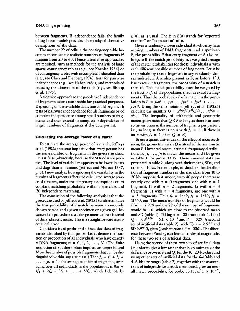
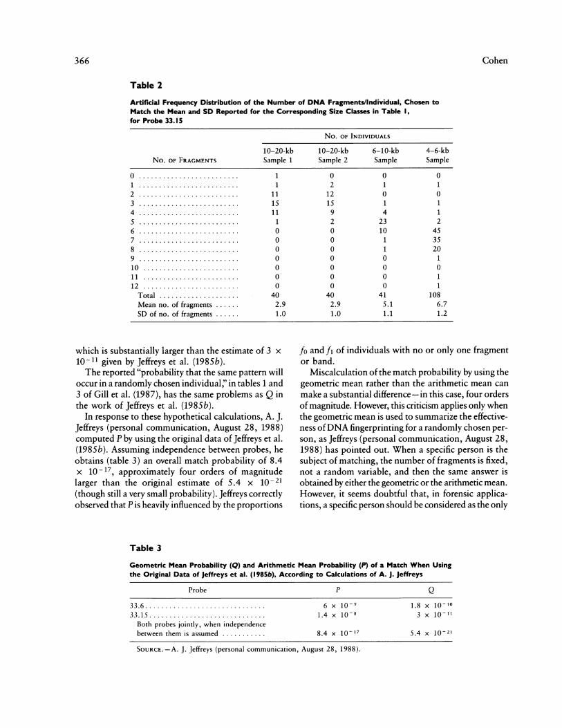
To get a quantitative idea of the effect of incorrectly using the geometric mean Q instead of the arithmetic mean P, I invented several artificial frequency distribu­tions lo, /t, ... ,/N to match the means and SDs given in table 1 for probe 33.15. These invented data are presented in table 2, along with their means, SDs, and other statistics. For example, to simulate the distribu­tion of fragment numbers in the size class from 10 to 20 kb, suppose that among every 40 people there were exactly one with n = 0 fragments, one with n = 1 fragment, 11 with n = 2 fragments, 15 with n = 3 fragments, 11 with n = 4 fragments, and one with n = 5 fragments. Thus lo = 1140, It = 1140, /2 = 11/40, etc. The mean number of fragments would be E(n) = 2.929 and the SD of the number of fragments would be 1.0, which are dose to the observed mean and SD (table 1). Taking x = .08 from table 1, I find Q = .082.929 = 6.1 x 10-4 and P = .029. A second set of artificial data (table 2), with E(n) = 2.925 and SD 0.9710, gives Q as before and P = .0061. The differ­ence between P and Q is at least an order of magnitude, for these two sets of artificial data.

Using the second of these two sets of artificial data (in order to give a low rather than high estimate of the difference between P and Q) for the 10-20-kb class and using other sets of artificial data for the 6-10-kb and 4-6-kb size ranges (table 2), together with the assump­tions of independence already mentioned, gives an over­all match probability, for probe 33.15, of 1 x 10- 7,

366 Cohen

Table 2

Artificial Frequency Distribution of the Number of DNA Fragments/Individual, Chosen to Match the Mean and SD Reported for the Corresponding Size Classes in Table I, for Probe 33.1 5

10-20-kb No. OF fRAGMENTS Sample

0 ......................... ••• 0. 0 0 0 0 ••• 0 0. 0 •• 0 •••••• 1

2 ......................... 11 3 ......................... 15 4 •••••••••••••••••••••••• 0 11 5 ••••••••• 0 •••••• 0 •••••••• 1 6 ........... ••••••••••••• 0 0 7 • 0. 0 ••••••• 0. 0 •• 0 0 0 0. 0 0 •• 0 8 ......................... 0 9 • • • • • • • • • • • • • • • • • • • • • 0 ... 0 10 •• 0 0 •• 0 •••••• 0 0. 0 ••••••• 0 11 .......... . . . . . . . . . . . . . . 0 12 . . . . . . . . . . . . . . . . . . . . . ... 0

Total . . . . . . ........... . . . 40 Mean no. of fragments . . . . .. 2.9 SD of no. of fragments ...... 1.0

which is substantially larger than the estimate of 3 x to- 11 given by Jeffreys et al. (1985b).

The reported "probability that the same pattern will occur in a randomly chosen individual;' in tables 1 and 3 of Gill et al. (1987), has the same problems as Q in the work of Jeffreys et al. (1985b).

In response to these hypothetical calculations, A. J. Jeffreys (personal communication, August 28, 1988) computed P by using the original data of Jeffreys et al. (1985b). Assuming independence between probes, he obtains (table 3) an overall match probability of 8.4 x 10- 17, approximately four orders of magnitude larger than the original estimate of 5.4 x to- 21

(though still a very small probability). Jeffreys correctly observed that Pis heavily influenced by the proportions

Table 3

1

No. OF INDIVIDUALS

10-20-kb 6-10-kb 4-6-kb Sample 2 Sample Sample

0 0 0 2

12 0 0 15 1 1

9 4 2 23 2 0 10 45 0 1 35 0 1 20 0 0 0 0 0 0 0 1 0 0 1

40 41 108 2.9 5.1 6.7 1.0 1.1 1.2

fo and /t of individuals with no or only one fragment or band.

Miscalculation of the match probability by using the geometric mean rather than the arithmetic mean can make a substantial difference-in this case, four orders of magnitude. However, this criticism applies only when the geometric mean is used to summarize the effective­ness of DNA fingerprinting for a randomly chosen per­son, as Jeffreys (personal communication, August 28, 1988) has pointed out. When a specific person is the subject of matching, the number of fragments is fixed, not a random variable, and then the same answer is obtained by either the geometric or the arithmetic mean. However, it seems doubtful that, in forensic applica­tions, a specific person should be considered as the only

Geometric Mean Probability (Q) and Arithmetic Mean Probability (I') of a Match When Using the Original Data of Jeffreys et al. (198Sb), According to Calculations of A. J. Jeffreys

Probe

33.6 ............................. . 33.15 ............................ .

Both probes jointly, when independence between them is assumed .......... .

p

6 X 10- 9

1.4 X 10- 8

8.4 X 10- 17

SouRCE.-A.]. Jeffreys (personal communication, August 28, 1988).

Q

1.8 X 10- 10

3 X 10- 11

5.4 X 10-Zt

DNA Fingerprinting

possible candidate for matching. If a given suspect is exonerated because his DNA fingerprint does not match that of a specimen, the police will not, in general, sim­ply stop looking for the criminal but will seek another person; when th-ey do seek another suspect, the num­ber of fragments in the person being compared to the specimen is indeed a random variable, and the arith­metic mean, not the geometric mean, is appropriate.

Conclusion

Scientific data and statistical analyses play increas­ing roles in the courtroom (DeGroot et al. 1986; Black 1988; Marx 1988). Increasingly, judges are requiring that the details of the evidence and the analysis be ex­plicit and well founded (Black 1988). It is the responsi­bility of scientists and statisticians to provide measure­ments, analyses, and conclusions that justify lawyers' faith in "relatively simple and well-defined techniques like electrophoresis or polygraph lie detection" (Black 1988, p. 1509). When such faith is not justified, it is scientists' responsibility to provide clear warning labels to the contrary. Since human lives and liberty are at stake in uses of DNA fingerprinting for forensic identification, it is important that there be little room for doubt about the assumptions underlying the analy­sis and interpretation of DNA fingerprinting data, in­cluding their statistical analysis and statistical interpre­tation.

The difficulty in establishing the statistical basis of DNA fingerprinting for forensic identification lies in assuring that the assumptions implicit in the calcula­tions are justified by evidence or theory and that any simplifying approximations made give conservative es­timates (i.e., overstatements) of match probabilities.

Some methods of statistical analysis of data on DNA fingerprinting suffer serious weaknesses. Unlinked Men­delizing loci that are at linkage equilibrium in subpopu­lations may be statistically associated, not statistically independent, in the population as a whole if there is heterogeneity in gene frequencies between subpopula­tions. In the populations where DNA fingerprinting is used for forensic applications, the assumption that DNA fragments occur statistically independently for differ­ent probes, different loci, or different fragment size classes lacks supporting data so far; there is some con­trary evidence. Statistical association of alleles may cause estimates based on the assumption of statistical independence to understate the true matching proba­bilities by many orders of magnitude. The assumptions that DNA fragments occur independently and with con­stant frequency within a size class appear to be con-

367

tradicted by the available data on the mean and vari­ance of the number of fragments per person. The mistaken use of the geometric mean instead of the arith­metic mean to compute the probability that every DNA fragment of a randomly chosen person is present among the DNA fragments of a specimen may substantially understate the probability of a match between blots, even if other assumptions involved in the calculations are taken as correct. The conclusion is that some astro­nomically small probabilities of matching by chance, which have been claimed in forensic applications of DNA fingerprinting, presently lack substantial empiri­cal and theoretical support.

Many of the above issues apply to paternity testing through DNA fingerprinting as well as to forensic identification of unrelated individuals. Because of the possible relatedness of individuals in paternity testing, the genetic formulas are more complicated than the for­mulas used in identifying unrelated individuals. How­ever, most of the underlying hypotheses are the same, and most of the same caveats apply.

Future experiments and analyses could provide a firmer foundation for DNA fingerprinting by giving careful attention to both sampling and possible statisti­cal dependence among fragments. DNA fingerprinting can be the basis of a useful method of identifying indi­viduals, provided that claims for it are not exaggerated.

Acknowledgments

I thank Jeffrey Glassberg for introducing me to DNA finger­printing and for suggesting this analysis. On a previous draft (dated June 1, 1988) I received comments from D. J. Boggs, S. E. Fienberg, P. Gill, J. Glassberg, W. Kruskal, J. Leder­berg, A. I. Sanda, and D. J. Werrett and very extensive written criticisms from A. J. Jeffreys. On a subsequent draft (dated July 12, 1989) I received very constructive comments from D. J. Boggs and two referees. Though I have done my best to benefit from their comments and criticisms, I do not in­tend to associate any of these commentators with any conclu­sions reached here. The inception of this work was supported in part by Lifecodes, Inc.; however, Lifecodes has had no influence on the conclusions reached. Subsequent develop­ment of the work has been supported in part by U.S. Na­tional Science Foundation grant BSR 87-05047, by the Insti­tute for Advanced Study (Princeton, NJ), and by the hospitality of Mr. and Mrs. William T. Golden.

References

Bishop YMM, Fienberg SE, Holland PW (197 5) Discrete mul­tivariate analysis: theory and practice. MIT Press, Cam­bridge, MA

368

Black B (1988) Evolving legal standards for the admissibility of scientific evidence. Science 239:1508-1512

Chen T, Fienberg S (1976) The analysis of contingency tables with incompletely classified data. Biometrics 32:133-144

Collaborative Research, Inc. (1989) Identification and par­entage testing using Collaborative Research DNA probes. Advertisement dated May 15, 1989. Collaborative Research, Inc., Bedford, MA

Crow JF, Kimura M (1970) An introduction to population genetics theory. Harper & Row, New York

DeGroot M, Fienberg SE, Kadane JB (eds) (1986) Statistics and the law. Wiley, New York

Fienberg SE (1980) The analysis of cross-classified categori­cal data, 2d ed. MIT Press, Cambridge, MA

Fienberg SE, Schervish MJ (1986) The relevance of Bayesian inference for the presentation of statistical evidence and for legal decisionmaking. Boston U Law Rev 66:771-798

Gill P, Lygo JE, Fowler SJ, Werrett DJ (1987) An evaluation of DNA fingerprinting for forensic purposes. Electropho­resis 8:38-44

Good IJ, Mittal Y (1987) The amalgamation and geometry of two-by-two contingency tables. Ann Stat 15:694-711

Gusella JF, et al (1983) A polymorphic DNA marker geneti­cally linked to Huntington's disease. Nature 306:234-238

Haber M (1986) Testing for pairwise independence. Biomet­rics 42:429-435

Haberman SJ (1974) The analysis of frequency data. Univer­sity of Chicago Press, Chicago

Jeffreys AJ, Morton DB (1987) DNA fingerprints of dogs and cats. Anim Genet 18:1-15

Jeffreys AJ, Royle NJ, Wilson V, Wong Z (1988) Spontaneous mutation rates to new length alleles at tandem-repetitive

Cohen

hypervariable loci in human DNA. Nature 332:278-281 Jeffreys AJ, Wilson V, Thein SL (1985a) Hypervariable "mini­

satellite" regions in human DNA. Nature 314:67-73 Jeffreys AJ, Wilson V, Thein SL (1985b) Individual-specific

"fingerprints" of human DNA. Nature 316:76-79 Jeffreys AJ, Wilson V, Thein SL, Weatherall DJ, Ponder BAJ

(1986) DNA "fingerprints" and segregation analysis of mul­tiple markers in human pedigrees. Am J Hum Genet 39: 11-24

Koehler KJ (1986) Goodness-of-fit tests for log-linear models in sparse contingency tables. JAm Stat Assoc 81:483-493

Kruskal W (1988) Miracles and statistics: the casual assump­tion of independence. J Am Stat Assoc 83:929-940

Lander ES (1989) DNA fingerprinting on trial. Nature 339:501-505

Lewin R (1989) DNA typing on the witness stand. Science 244:1033-1035

MarxJL (1988) DNA fingerprinting takes the witness stand. Science 240:1616-1618

Sensabaugh G, Witkowski J (1989) DNA technology and forensic science. Banbury rep 32. Cold Spring Harbor Lab­oratory, Cold Spring Harbor, NY

Snedecor GW, Cochran WG (1980) Statistical methods, 7th ed. Iowa State University Press, Ames

Tribe L (1971) Trial by mathematics: precision and ritual in the legal process. Harvard Law Rev 84:1329-1393

Wong Z, Wilson V, Patel I, Povey S, Jeffreys AJ (1987) Char­acterization of a panel of highly variable minisatellites cloned from human DNA. Ann Hum Genet 51:269-288

Yule GU (1903) Notes on the theory of association of attri­butes in statistics. Biometrika 2:121-134