Diversification and Efficiency of Investment

By East Asian Corporations

Stijn Claessens*, Simeon Djankov*, Joseph P.H. Fan**, and Larry H.P. Lang***

* World Bank** Hong Kong University of Science and Technology

*** The University of Chicago

The opinions expressed do not necessarily reflect those of the World Bank. We thank Jack Glen,Joel Houston, Guy Pfeffermann, Rene Stulz, and seminar participants at the World Bank, theFederation of Thai Industry in Bangkok, KDI in Korea, and the 1998 World Bank conference inKuala Lumpur for helpful suggestions. For comments, please contact Simeon Djankov, tel 202 4734748; EM: sdjankov@worldbank.org

1

Diversification and Efficiency of InvestmentBy East Asian Corporations

Stijn Claessens, Simeon Djankov, Joseph P.H. Fan, and Larry H.P. Lang

1. Introduction

The East Asian financial crisis has at least in part been attributed to the extensive

diversification of corporates, which is associated with misallocation of capital investment

towards less profitable and more risky business segments. While a plethora of anecdotal

evidence to support this argument has surfaced in the aftermath of the crisis, there was little

discussion preceding the crisis. Quite the opposite, the rapid expansion of East Asian

corporations through entry into new business segments was seen as an important

contributing factor to the East Asian Miracle (World Bank (1994)). In this paper, we

examine the efficiency of investment by diversified corporations in nine East Asian

countries, using unique panel data of more than 10,000 firms over the 1991-96 pre-crisis

period. We offer three contributions to the literature. First, we document the degree of

diversification on the corporate sector in Hong Kong, Indonesia, Japan, Korea, Malaysia,

the Philippines, Singapore, Taiwan, and Thailand, countries which have achieved enviable

rates of economic growth over the last three decades. Second, we distinguish between

vertical and complementary diversification and study the differences across the nine

countries. Finally, we investigate whether diversification in East Asia has hurt economic

efficiency.

To accomplish the first two contributions, we use the inter-industry commodity

flow data in the US input-output table as a common benchmark to construct vertical

relatedness and complementarity indices between the primary and the secondary businesses

of all sample firms in the nine countries (see Fan, Lang and Stulz (1998)). These measures

allow us to describe, for any pairs of businesses, the possibility of vertical integration, joint

procurement, and/or sharing marketing and distribution in each firm. We document the

degree of diversification in the corporate sector, distinguish between vertical and

complementary diversification, and study the differences across the nine countries.

2

We use two competing hypotheses to help answer the third question. The

misallocation-of-capital hypothesis states that diversified firms allocate capital to less

profitable segments. The more diverse and complex the investment opportunities available,

the more pronounced this misallocation is.1 Such misallocation of capital should be

associated with a reduction of short-term profitability and a pronounced diversification

discount. In contrast, the learning-by-doing hypothesis argues that when firms diversify

into new lines of business, there is an initial period during which labor is learning how to

use the new technology, and a reduction in short-term profitability should be observed.2

This learning-by-doing should not be associated, however, with a diversification discount

since the forward-looking capital market fairly assesses the increase in profitability over

time as the learning-by-doing pays off. We test these hypotheses by separating vertical and

complementary diversification. Since vertical diversification is more complex in

technology, management, and capital investment than complementary diversification (and

thus involves more possibilities for misallocation of capital and learning-by-doing), we

should observe a more pronounced effect on short-term profitability and diversification

discount in vertical diversification than in complementary diversification.3

Our East Asian sample allows us to effectively test these two competing

hypotheses. First, some governments in the region have encouraged corporations to engage

in vertical expansion to upgrade technology and general level of development (see World

Bank (1998)). Since this is not a pure market-outcome, it may be more likely to find a

differential effect of vertical integration and complementary diversification for countries

with heavy intervention such as South Korea than for countries undertaking a natural

transition into diversified businesses. Second, the nine East Asian countries are at different

levels of development, which provides insights into the link between diversification

patterns and outcomes and the general level of economic development.4 This diversity

1 See Shin and Stulz (1996), Scharfstein (1997), and Rajan, Servaes, and Zingales (1997).2 See Stockey (1991) and Young (1993).3 See discussion of vertical integration in Williamson (1971) and Klein, Crawford and Alchian (1978).4 In particular, the nine countries can be thought of as a V-formation with Japan at the lead, flanked by HongKong, Singapore and Taiwan, then South Korea, Malaysia and finally Thailand, Indonesia and thePhilippines.

3

allows us to test the differential effect of vertical integration and complementary

diversification by level of development.5

We find that Indonesia, South Korea, Taiwan and Thailand have suffered

significant negative impact of vertical integration on profit margins, while the same four

countries have seen significant benefits from complementary expansion on profit margins.

In contrast, the diversification discount results suggest that the negative impact of vertical

diversification only remains for South Korea and Malaysia. It suggests that the

misallocation of capital is more pronounced in South Korea and possibly Malaysia than in

Indonesia, Taiwan and Thailand, while the learning hypothesis is more pronounced for

these three countries.

The diversity of economic development in our East Asian samples allows us to

further examine these two hypotheses by investigating the link between diversification

effects and the level of economic development of a country. We would expect that the

learning and capital misallocation problems are sensitive to the degree of economic

development of the country to which a firm belongs. Consistent with the learning-by-doing

hypothesis, firms in more developed countries are successful in vertically integrating with

lower costs to both short-term profitability and market valuation since they already make

use of sophisticated technologies and may have peer firms to learn from. In contrast, firms

in less developed countries benefit more from complementary diversification, but firms in

more developed countries are more likely to ultimately benefit from such diversification.

This is also consistent with the learning-by-doing hypothesis where firms in more

developed countries go faster up their learning curves and improve their performance. We

also find evidence consistent with the misallocation-of-capital hypothesis, as diversification

by firms in less developed countries is subject to more misallocation of capital. Our

evidence supports the finding in Shin and Stulz (1996) that internal capital markets play a

more important role in less developed countries, however the internal capital markets

misallocate capital. On the other hand, capital misallocation is less relevant to firms in

more developed countries, as there is no evidence of a pronounced diversification discount

for firms in more developed countries.

5 For example, Japan is the most developed country, for example, vertical integration should involve lesscosts of misallocation of capital and learning-by-doing than the other countries.

4

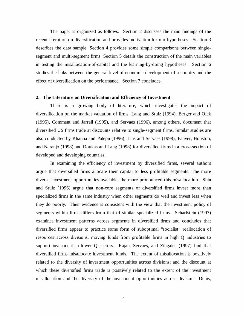
The paper is organized as follows. Section 2 discusses the main findings of the

recent literature on diversification and provides motivation for our hypotheses. Section 3

describes the data sample. Section 4 provides some simple comparisons between single-

segment and multi-segment firms. Section 5 details the construction of the main variables

in testing the misallocation-of-capital and the learning-by-doing hypotheses. Section 6

studies the links between the general level of economic development of a country and the

effect of diversification on the performance. Section 7 concludes.

2. The Literature on Diversification and Efficiency of Investment

There is a growing body of literature, which investigates the impact of

diversification on the market valuation of firms. Lang and Stulz (1994), Berger and Ofek

(1995), Comment and Jarrell (1995), and Servaes (1996), among others, document that

diversified US firms trade at discounts relative to single-segment firms. Similar studies are

also conducted by Khanna and Palepu (1996), Lins and Servaes (1998), Fauver, Houston,

and Naranjo (1998) and Doukas and Lang (1998) for diversified firms in a cross-section of

developed and developing countries.

In examining the efficiency of investment by diversified firms, several authors

argue that diversified firms allocate their capital to less profitable segments. The more

diverse investment opportunities available, the more pronounced this misallocation. Shin

and Stulz (1996) argue that non-core segments of diversified firms invest more than

specialized firms in the same industry when other segments do well and invest less when

they do poorly. Their evidence is consistent with the view that the investment policy of

segments within firms differs from that of similar specialized firms. Scharfstein (1997)

examines investment patterns across segments in diversified firms and concludes that

diversified firms appear to practice some form of suboptimal “socialist” reallocation of

resources across divisions, moving funds from profitable firms in high Q industries to

support investment in lower Q sectors. Rajan, Servaes, and Zingales (1997) find that

diversified firms misallocate investment funds. The extent of misallocation is positively

related to the diversity of investment opportunities across divisions; and the discount at

which these diversified firms trade is positively related to the extent of the investment

misallocation and the diversity of the investment opportunities across divisions. Denis,

5

Denis and Sarin (1997) argue that these value-reducing investment strategies are sustained

over time because they benefit management, but a competitive corporate control market

may act as a disciplining tool. The ineffective corporate control market in the mid-1980s

has exacerbated this inefficiency (Jensen (1986, 1989)).

The misallocation-of-capital argument is complementary to the observation by

Stockey (1991) and Young (1993) who argue that when firms diversify into new

businesses, the diversification is associated with a temporarily lower level of profitability

as the firm is learning to use the new technology. If the capital is used for advantageous

economic activity, however, profitability should recover over time. Young (1992, 1995)

has applied the learning-by-doing hypothesis in the diversification context of East Asia,

examining the patterns of corporate growth in Hong Kong and Singapore. He finds that as

firms diversify into less related businesses, they require more time to adapt to the new

technology (see also Kim and Lau (1994) and Krugman (1994)). Since corporations in

Singapore are given incentives by the government to rapidly move into more technology-

intensive sectors, they can seldom reach a sufficient level of learning before embarking on

a new venture.

A third literature is related to the internal capital market of diversified firms. When

external capital markets are more costly to use, firms allocate their capital internally

through diversification (Williamson (1971), Gertner, Scharfstein and Stein (1994), Lamont

(1997), Stein (1997), Scharfstein and Stein (1997) and Scharfstein (1998)). Fauver,

Houston, and Naranjo (1998) find that diversified firms perform better when the capital

markets and the legal systems of their country are less developed. Following the internal

capital market hypothesis, diversification within firms is an efficient response to the

distortions in the external environments or weak external financial markets. However, as

argued by Shin and Stulz (1996), internal capital markets may lead to misallocation of

capital due to the heterogeneous and complex investment opportunities across the segments

of the firms.

6

3. The Data

We study corporate diversification in nine countries: Hong Kong, Indonesia, South

Korea, Japan, Malaysia, Philippines, Singapore, Taiwan and Thailand.6 Our primary data

source is the Worldscope database. Worldscope contains financial and segment information

on companies from 49 countries. The database has been used in several international

studies of corporate diversification (Lins and Servaes (1997) and Fauver, Houston, and

Naranjo (1998)).

We initially selected all companies from the nine countries covered by the June

1991-1998 CD-Rom version of annual Worldscope database. In each of the annual

database, Worldscope provides historical financial data. We are able to assemble several

years of financial data for most of the companies. Historical segment data for many of the

companies are missing, however, since Worldscope reports only the latest available

segment data. To increase sample size, we collected additional segment data for

Worldscope companies from the autumn edition of the 1994-1998 Asian Company

Handbook and Japan Company Handbook. All financial data were converted to US dollars

using fiscal year end foreign exchange rate for each firm.

In order to determine the types of the companies’ businesses, we group the

companies’ segments according to the two-digit Standard Industry Classification (SIC)

system. This procedure involves two steps. In the first step, we assign the four-digit SIC

codes reported by Worldscope to appropriate segments. In many cases we are able to

obtain one-to-one matches between SIC codes and segments. For some companies, the

number of reported SIC codes is not the same as the number of reported segments. If a

segment can not be associated with a reported SIC code, we determine the segment’s SIC

code according to its business description. If a segment is associated with multiple SIC

codes, it is broken down equally so that each segment is associated with one SIC code. In

the second step, we redefine segments at the two-digit SIC level and aggregate segment

sales to that level.

We classify firms as single-segment if at least 90 percent of their total sales are

derived from one two-digit SIC segment. Firms are classified as multi-segment if they

6 Although China is also an interesting case, we can locate only a handful public firms from Worldscope. Thedominant corporate units in China are state-owned enterprises. The few publicly traded firms are far fromrepresentative of the census of firms in China.

7

operate in more than one two-digit SIC code industries and none of their two-digit SIC

code segments accounts for more than 90 percent of total firm sales.7 This classification

scheme is the same as in Lins and Servaes (1996, 1997) and Fauver, Houston, and Naranjo

(1998). We further define the primary segment of a multi-segment firm as the largest

segment by sales. The remaining segment(s) are defined as secondary segments. In a

small number of cases two largest segments have identical sales. In such cases we select

the segment with the lower two-digit SIC code as the primary segment. Note that our

empirical results generally hold if the alternative is chosen as the primary segment.

Following Lins and Servaes (1997, 1998) and Fauver, Houston, and Naranjo

(1998), we exclude multi-segment firms from the sample when they do not report segment

sales. We also exclude firms whose primary business segment is financial services (SIC

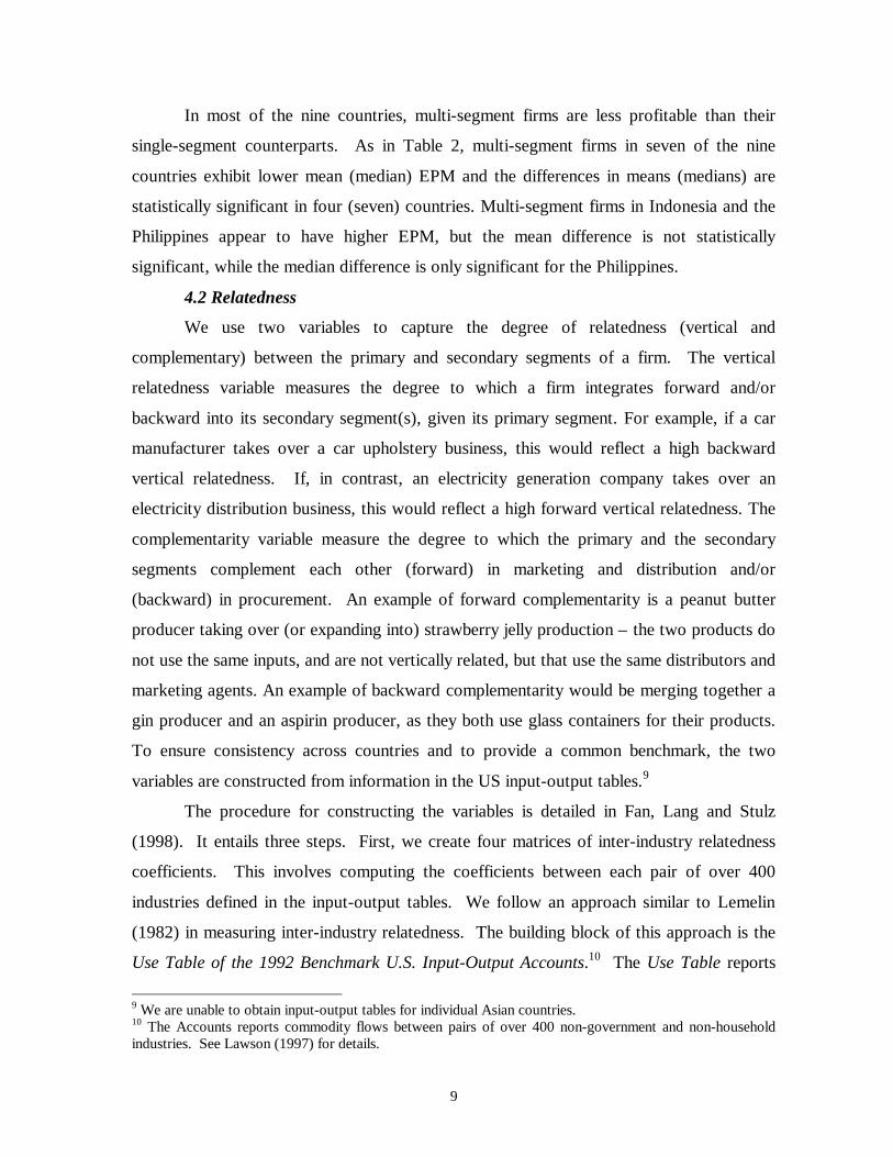
6000-6999). This selection results in a sample described in Table 1.

[Table 1 here]

There are 8,450 (65%) multi-segment firms and 4,625 (35%) single-segment firms

in the sample. Japanese firms comprise the majority of the sample, as they account for 75

percent of the multi-segment firms and 68 percent of the single-segment firms. Across the

nine countries, Singapore and Malaysia rank high in the percentage of multi-segment firms

(72 and 70 percent, respectively), while Thailand and the Philippines have the lowest

percentage (27 and 33 percent, respectively).

The average size of multi-segment firms is US$2,371 million in total assets and

US$1,776 million in total assets for single-segment firms. Across the nine countries, the

average assets of multi-segment firms are mostly larger than those of single-segment firms,

with the exception of South Korea and Singapore. Of the multi-segment firms, Japanese

firms have the largest average assets (US$2,850 million), followed by Korean and Hong

Kong firms. Of the single-segment firms, Korean firms have the largest average assets

(US$2,250 million), followed by Japanese and Hong Kong firms.

7 We also use 80% cut-off as a robustness check. The qualitative results do not change.

8

4. Construction of the Main Variables

4.1 Short-term Performance

To examine the hypothesis by Shin and Stulz (1996) that investment policy of

segments in diversified firms differs from that of similar specialized firms, we employ the

“chop-shop” procedure of Lang and Stulz (1996) to construct our short-term and long-term

performance measures. In addition to adjust for sectoral differences in performance, the

measures can be interpreted as the performance of a multi-segment firm relative to single-

segment firms in its industries. These measures allow us to compare the performance

differences between multi-segment (diversified) and single-segment (focused) firms and

associate the performance differences with their different investment strategies.

We measure a firm’s short-term performance by its profit margin, calculated as one

minus the costs of goods sold over sales. We first use the sub-sample of single-segment

firms in each country to compute the median profit margin for each two-digit SIC code

industry. We then multiply the sales share in each segment of a firm by the corresponding

industry median profit margin. We sum the sales-weighted profit margin across segments

to obtain the imputed profit margin of the firm. Lastly, we subtract the imputed profit

margin from the actual profit margin to obtain the industry-adjusted excess profit margin

(EPM).8

In the computation of industry median profit margin, we restrict the number of

single-segment firms to be at least three. In some cases, we do not have sufficient number

of firms to compute the median profit margin. In these cases, we use the median profit

margin of broader industry groups as defined by Campbell (1996). This procedure avoids

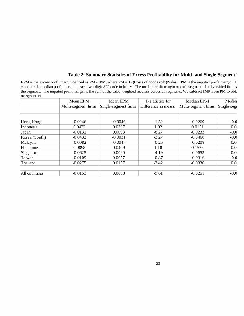
the loss of observations. Table 2 compares the differences in the excess profit margin

measures between single- and multi-segment firms. Overall, multi-segment firms are less

profitable than single-segment firms. The difference in mean and median EPM between the

multi- and single-segment firms is negative and statistically significant at the 1-percent

level.

[Table 2 here]

8 The excess profit margin is more appropriate than other accounting income variables for the purposes of thisstudy, since it is perfectly correlated with average variable cost (defined as 1 – profit margin) which is widelyused by micro economists to proxy factor productivity changes (see, for example, Young (1992) and Clerides,Lach and Tybout (1998)).

9

In most of the nine countries, multi-segment firms are less profitable than their

single-segment counterparts. As in Table 2, multi-segment firms in seven of the nine

countries exhibit lower mean (median) EPM and the differences in means (medians) are

statistically significant in four (seven) countries. Multi-segment firms in Indonesia and the

Philippines appear to have higher EPM, but the mean difference is not statistically

significant, while the median difference is only significant for the Philippines.

4.2 Relatedness

We use two variables to capture the degree of relatedness (vertical and

complementary) between the primary and secondary segments of a firm. The vertical

relatedness variable measures the degree to which a firm integrates forward and/or

backward into its secondary segment(s), given its primary segment. For example, if a car

manufacturer takes over a car upholstery business, this would reflect a high backward

vertical relatedness. If, in contrast, an electricity generation company takes over an

electricity distribution business, this would reflect a high forward vertical relatedness. The

complementarity variable measure the degree to which the primary and the secondary

segments complement each other (forward) in marketing and distribution and/or

(backward) in procurement. An example of forward complementarity is a peanut butter

producer taking over (or expanding into) strawberry jelly production – the two products do

not use the same inputs, and are not vertically related, but that use the same distributors and

marketing agents. An example of backward complementarity would be merging together a

gin producer and an aspirin producer, as they both use glass containers for their products.

To ensure consistency across countries and to provide a common benchmark, the two

variables are constructed from information in the US input-output tables.9

The procedure for constructing the variables is detailed in Fan, Lang and Stulz

(1998). It entails three steps. First, we create four matrices of inter-industry relatedness

coefficients. This involves computing the coefficients between each pair of over 400

industries defined in the input-output tables. We follow an approach similar to Lemelin

(1982) in measuring inter-industry relatedness. The building block of this approach is the

Use Table of the 1992 Benchmark U.S. Input-Output Accounts.10 The Use Table reports

9 We are unable to obtain input-output tables for individual Asian countries.10 The Accounts reports commodity flows between pairs of over 400 non-government and non-householdindustries. See Lawson (1997) for details.

10

for each pair of industries i and j the dollar value of i’s output required to produce industry

j’s total output, denoted as Vij. We divide Vij by the dollar value of industry j’s total

output to get vij, representing the dollar value of i’s output required to produce one dollar

worth of industry j’s output. When vij is large, it suggests a high degree of forward

integration of i into j. Conversely, vji measures the dollar value of j’s product required by

industry i to produce one dollar worth of its output. When vji is large, it suggests an

opportunity for i to backward integrate into j. We therefore define two vertical relatedness

coefficients, FVRij=vij and BVRij=vji, to proxy for the opportunity for industry i to

forward and backward integrate into industry j, respectively.

From the Use Table, we compute for each industry i the percentage of its output

supplied to each industry k, denoted as cik. For each pair of industry i and j, we compute

the simple correlation coefficient between cik and cjk across all k. A large correlation

coefficient in the percentage output flows suggests a significant overlap in markets to

which industry i and j sell their products.11 For each pair of industry i and j, we also

compute a simple correlation coefficient across industry input structures between the input

requirement coefficients vik and vjk of the two industries. A large correlation coefficient

suggests a significant overlap in inputs required by industries i and j. We hence define two

complementarity coefficients, FCOMij = corr(cik, cjk) and BCOMij = corr(vik, vjk), to

proxy for the degree of forward and backward complementarity between industries i and j,

respectively. Trade between I and j is excluded from the correlations. In step one, the

subscripts for FVR, BVR, FCOM, and BCOM are small i and j which denote 400x400

industries.

In the second step, we condense the relatedness coefficient matrices to

accommodate the widely used SIC codes and reduce 400 industries to a manageable

number. This involves classifying the industries into 34 industry groups and computing

mean relatedness coefficients by pairs of industry groups. For each pair of the 34 industry

groups, we compute mean relatedness coefficients across pairs of industries that are

classified into the same 34 pairs of industry groups. This results in four 34x34 matrices of

mean relatedness coefficients.

11 This coefficient is not used in the Lemelin (1982) study.

11

In the third step, we construct the relatedness variables for each multiple-segment

firms in our sample based on the mean relatedness coefficients from the condensed

matrices. We define the vertical relatedness and the complementarity variables as follows.

V = Σk(wk*FVRkIJ) + Σk(wk*BVRk

IJ), and

C = Σk(wk*FCOMkIJ) + Σk(wk*BCOMk

IJ),

where wk is the sales weight equal to the ratio of the kth secondary segment assets to the

total assets of all secondary segments; FVRkIJ, BVRk

IJ, FCOMkIJ, and BCOMk

IJ are the

four mean related coefficients associated with industry group I and J to which the primary

and the secondary segments belong.

[Table 3 here]

In Table 3, we rank multi-segment firms by their relatedness levels, group the firms

into ten percentiles, and compute mean relatedness measures for each of the ten percentiles.

We focus on the 50th (median) percentile. The mean vertical relatedness is 0.0049 (Table

3, Panel A). This implies that for every dollar worth of production by the firm, only 0.49

cent is potentially transacted in-house between the primary and secondary segments. The

maximum in-house transaction is 10 cent per dollar worth of output, while the minimum is

zero. Across the nine countries, the mean vertical relatedness of the 50 percentile is

highest for Thailand (0.0096), followed by Indonesia, Singapore, Hong Kong, Malaysia,

the Philippines, Japan, Korea, and Taiwan (0.0031). This order does not correlate with the

degree of economic development.

Panel B of Table 3 reports mean complementarity measures by percentile. The

mean complementarity of the 50th percentile is 0.3413. The maximum is 2 while the

minimum is close to zero. Comparing the levels of the two relatedness measures, these

numbers suggest that the across-industry diversification by the Asian companies generate

more opportunities of sharing procurement and/or sales activities relative to the opportunity

of transacting input internally through vertical integration. Across the nine countries, the

mean complementarity of the 50th percentile is the highest for Singapore (0.3991), followed

by Hong Kong, Thailand, Japan, South Korea, Indonesia, Taiwan, the Philippines, and

Malaysia (0.2091). This order does not appear to correlate with the across-country order of

the vertical relatedness measure or the degree of economic development.

12

To further examine the patterns of diversification by the firms, we report in Panel A

and B of Table 4 the distribution of firms by number and by cumulative percentage across

ten different levels of the vertical relatedness measure V. As in Panel A and B, the

majority of the multi-segment firms falls into the category of V<0.01. For the sample as a

whole, 5,298 (70%) of firms have their vertical relatedness measure below that level. The

number of firms decreases as V increases. The pattern suggests that, for most of the firms,

there exist a small amount of transactions (less than 1 cent per dollar of output) between the

firms’ primary and secondary segments.

[Table 4 here]

Across the nine countries, Thailand has the lowest percentage (50%) of firms

falling into the first category where V<0.01, followed in ascending order by Hong Kong,

Singapore, Indonesia, Philippines, Malaysia, Japan, South Korea, and Taiwan (86%). The

order is almost identical to the results presented in Table 3. The order suggests that Thai-

firms have more vertically-related segments than firms in the eight other countries. On the

other hand, Taiwanese multi-segment firms are the least vertically related.

Panel C and D of Table 4 present the distribution of firms across ten levels of the

complementarity measure C which indicates the possibility of sharing procurement or sales

activities. In the sample as a whole, the majority (62%) of the multi-segment firms falls

into the first four categories where C<0.4. Using 0.4 as the cutoff level, the countries in

ascending order of the cumulative percentage are Singapore (50%), Hong Kong (52%),

Indonesia (59%), Thailand (60%), Japan (61%), Taiwan (73%), Philippines (75%), Korea

(76%), and Malaysia (77%). The order is comparable to the results in Table 3, with

Singaporean firms having the highest segmental complementarity, and Malaysian firms

having the least segmental complementarity.

4.3 Diversification Discount

In calculating the diversification discount, we adopt the approach of Berger and

Ofek (1995) and extended by Lins and Servaes (1997, 1998) and Fauver, Houston, and

Naranjo (1998) to the international context. This approach defines the excess value of the

diversification discount (EXV) as the ratio of the firm’s actual value to its imputed value.

Market capitalization is used as the measure of actual firm value. It is the market value of

common equity plus the book value of debt. The imputed value is computed following the

13

industry-matching scheme described in Section 4.1. We first compute median market-to-

sales ratio for each industry in each country using only single-segment firms. The market-

to-sales ratio is the market capitalization divided by firm sales. We then multiply the level

of sales in each segment of a firm by its corresponding industry median market-to-sales

ratio. The imputed value of the firm can be obtained by summing the multiples across all

segments. We also restrict the number of single-segment firms to at least three when

computing the median market-to-sales ratio of an industry. When an industry has fewer

than three single-segment firms even defined broadly as Campbell (1996), we use the

median of all firms in the country.

5. Regression analysis

5.1 Relatedness and short-term performance

To be consistent with both hypotheses, we should observe a differential effect

between vertical and complementary diversification on EPM. We test this proposition by

performing the following estimation:

EPM = a + b1*V + b2*C + b3*SEGN + b4*Log(ASSETS) + (Fixed effects) + u

where EPM is the industry-adjusted excess profit margin, V is the vertical relatedness

measure, and C is the complementarity measure. The explanatory variables also include

the number of firm segments (SEGN) and the natural logarithm of firm assets in thousands

of US dollars (Log(ASSETS)) to control for segment and size effects.12 Lastly, we include

country and year dummy variables to control for any fixed effects that may exist. The

regression is performed on the pooled sample of multi-segment firms as well as on country-

by-country samples.

[Table 5 here]

Table 5 presents the regression results. In the pooled regression, the estimated

coefficients of the two relatedness variables V and C are both positive but only the latter is

statistically significant. The result is largely driven by Japanese firms, which account for

12 Morck, Shleifer and Vishny (1988) argue that firm size should be included as a control variable since thesize may be correlated with value. In this study, we control for the size effect because the diversificationstrategy would increase the size of a firm, which increases the inefficiency of running a bigger corporation.

14

more than two third of the sample. In the country-by-country regressions, the estimated

coefficient of V is negative in all countries but Japan. The negative coefficients are

significant for Indonesia (significant at the 10% level), Korea (1%), Taiwan (5%), and

Thailand (5%). Vertical relatedness seems to hurt performance in these countries. Japan is

the only country whose profitability has benefited from vertical relatedness, as the

estimated coefficient of V is positive and significant at the 1-percent level.

In contrast, the estimated coefficient of C is positive in all but two countries, Hong

Kong and Japan. The positive coefficients are significant for Indonesia (5%), Korea (1%),

Taiwan (1%), and Thailand (1%). Firm profitability in these countries has thus benefited

from complementary diversification. Although the coefficients of C in the cases of Hong

Kong and Japan are negative, they are not statistically significant.

We next examine the effects of multiple segments on EPM. The coefficient of

SEGN is negative and significant, suggesting that more segments hurt firm profitability.

Across the nine countries, six countries exhibit negative segment effects and five of the

coefficient estimates are statistically significant. The Philippines is the only country

exhibiting significantly positive segment effect. This result may be driven by the small

sample size (35 firms). Lastly, there exist significant positive size effects on profitability

except for Taiwan. Large firms are on average more profitable than small firms, as

indicated by the positive and highly significant coefficient of Log(ASSETS) in the pooled

regression. The country-by-country evidence is consistent with the pooled result.

To provide the statistical significance of the difference of impact between vertical

and complementary diversification on profit margin, we test whether the estimated

coefficients of V and C from the regressions are equal. As reported in Table 5, the F-value

is not significant for the pooled sample. Across the nine countries, we find that the F-value

is significant in five countries: Indonesia, Japan, Korea, Taiwan, and Thailand. The

evidence for these four countries except for Japan is consistent with both hypotheses. Note

that Japan is the only country whose profitability has benefited from vertical relatedness

and the estimated coefficient of V is significantly higher than that of C. This evidence

indicates that Japan as the most developed country in East Asia may already utilize

sophisticated technologies and may also have peer firms to learn from. Hence they have

benefited from vertical diversification more than from complementary diversification

15

whose degree of required learning is low. We are unable to test this proposition in this

section, however it clearly indicates that the degree of economic development matters in

testing these two competing hypotheses. We will examine this issue in Section 6.

Note that if both vertical and complementary diversification have positive impact

on profitability, then it demonstrates that conglomerate diversification hurts profitability

more than related diversification. However, the impact between vertical and

complementary diversification on EPM should still be significantly different since vertical

diversification is more complex than complementary diversification. As we can see from

previous tables, vertical integration has a negative impact on most countries, while

complementary expansion has a positive impact on almost all countries. This evidence

suggests that vertical integration is indeed associated with a more complex structure in

technology, management and capital investment than complementary or possibly

conglomerate diversification.

5.2 Relatedness and diversification discount

The results in Section 5.1 show a significant differential effect for four countries

between vertical and complementary diversification. To be consistent with the learning

hypothesis, the diversification discount should not be affected by the degree of vertical

diversification. In contrast, to be consistent with the misallocation-of-capital hypothesis,

the diversification discount should be negatively significant for vertical diversification. To

test these two hypotheses, we perform the following estimation:

EXV = a + b1*V + b2*C + b3*SEGN + b4*Log(ASSETS) + (Fixed effects) + u

where EXV is the excess value of diversification discount, V is the vertical relatedness

measure, and C is the complementarity measure. The explanatory variables also include

the number of firm segments (SEGN) and the natural logarithm of firm assets in thousands

of US dollar (Log(ASSETS)) to control for segment and size effects. Lastly, we include

country and year dummy variables to control for any fixed effects that may exist. The

regression is performed on the pooled sample of multi-segment firms as well as on country-

by-country samples.

Table 6 presents the regression results. In the pooled regression, the estimated

coefficients of the two relatedness variables V and C are both positive and statistically

16

significant. In the country-by-country regressions, the estimated coefficient of V is

negative for only five countries. The negative coefficients are significant only for Korea

(5%) and Malaysia (5%). Japan is the only country whose EXV benefits from vertical

relatedness, as the estimated coefficient of V is positive and significant at the 1-percent

level. In contrast, the estimated coefficient of C is positive only for four countries, and

significant only for Japan (1%), South Korea (5%) and Singapore (5%).

[Table 6 here]

We next examine the effects of multiple segments on EPM. The coefficient of

SEGN is mixed. Only Japan exhibits a positive and significant effect, while Malaysia

experiences a negative and significant effect. Lastly, there exist significant positive size

effects on EXV except for Taiwan. Large firms are on average more profitable than small

firms. Note that these two variables have little relevance with the test of the two

hypotheses.

We study separately the significance levels of V on EXV for Indonesia, Korea,

Taiwan and Thailand since the results for EPM for these four countries are consistent with

both hypotheses. To be consistent with the learning hypothesis, the significant differential

effect between V and C should reduce or disappear. As documented in Table 6, the

statistical significance of the difference of impact between vertical and complementary

diversification on EXV is insignificant for three countries, Indonesia, Taiwan and Thailand.

In contrast, to be consistent with the misallocation-of-capital hypothesis, the significant

differential effect between V and C should remain, as is the case for South Korea. As

documented in Table 6, the statistical significance of the difference of impact between

vertical and complementary diversification on EXV is significant at the 5 % level for South

Korea.

The results for Malaysia are interesting. In the EPM regression, the effect of

vertical diversification on EPM is negative but insignificant, while this variable becomes

significantly negative and significantly different from the effect of complementary

diversification in the EXV regression. We may argue that Malaysia is a relatively less

developed country in East Asia. Its vertical integration may involve less complex layer of

technology, management and capital investment than in Korea or Taiwan, hence it may

impose less strain on short-term performance. However, Malaysia may have a more serious

17

misallocation of capital problem, which is reflected in the EXV regression. We hence

argue that the evidence is more consistent with the misallocation-of-capital hypothesis.

6. Diversification Effects and Economic Development

In this section, we study the two competing hypotheses by examining the link

between diversification effects and the level of economic development of a country. We

investigate whether the learning and capital misallocation problems are sensitive to the

degree of economic development of the country to which a firm belongs.

6.1 The learning-by-doing hypothesis

In previous section, using Japan as an example, we argued that learning-by-doing is

less costly for firms in more developed countries. Since vertical integration involves more

learning than complementary diversification, we should observe that firms in more

developed countries benefit more from vertical integration, because they already utilize

sophisticated technologies and may have peer firms to learn from. On the other hand, we

should not observe such performance difference for complementary diversification,

because the degree of required learning is low.

We regress EPM and EXV on diversification variables as well as variables

proxying the level of economic development of each of the nine countries. In the first

model specification, we use the average per-capita GNP13 during 1991-96 (World Bank

(1996)) as the proxy for economic development. In an alternative specification, we proxy

the level of economic development by using the World Bank classification of countries by

income level groups. This income grouping has been used in the studies of La Porta et al

(1998) and Fauver et al (1998). As reported by the World Bank, the lower-middle income

dummy equals one if the firm is from Indonesia, the Philippines, or Thailand. The high

income Dummy equals one if the firm is from Hong Kong, Japan, Singapore or Taiwan.

The numeraire is higher-middle income countries (Korea and Malaysia). The results are

reported in Table 7.

[Table 7 here]

13 We divide the per-capita GNP by 1,000,000 in the regressions.

18

Initially focus on the interactive effects of vertical relatedness and economic

development. From columns (2) and (4), the interaction term between Per-Capita GNP and

vertical relatedness is positive and significant for both EPM and EXV. From columns (1)

and (3), EPM and EXV are positively related to vertical relatedness in high-income

countries while negatively (or insignificantly in the case of EXV) related to it in lower-

middle income countries. These results suggest that firms in more developed countries are

successful in vertically integrating with lower costs to both short-term profitability and

market valuation, while this is not the case for firms in less-developed countries. We have

found support for the learning-by-doing hypothesis.

From Table 7, we observe differential short- and long-term interactive effects of

complementary diversification and economic development. From column (2) and (4), the

coefficient of (Per-Capita GNP)xC is significantly negative for the EPM regression but

significantly positive for the EXV regression. Using the alternative specification, the

coefficients of (Lower-income dummy)xC and (High-income dummy)xC in the EPM

regression are significantly positive and negative, respectively (column (1)). But the

reverse is true in the EXV regression (column (4)). From these results, it appears that in

the short run firms in less developed countries benefit more from complementary

diversification relative to those from more developed countries. It is consistent with the

view that, relative to more developed countries, the less developed countries are less open

and less competitive, they have more opportunities for short-term profits. But the firms in

more developed countries are more likely to ultimately benefit from such diversification.

This long-run result is consistent with the learning-by-doing hypothesis where firms in the

relatively more developed countries go faster up their learning curves and improve their

performance.

6.2 The misallocation-of-capital hypothesis

We next examine whether the firms’ diversification performance can be attributed

to misallocation of capital. We focus on the effects of vertical diversification on both the

short-term and long-term performance. From column (1) to column (4) of Table 7, the

estimated coefficients of V are negative and mostly significant, indicating the possibility of

misallocation of capital. The coefficients of Per-Capita GNPxV in column (2) and (4) are

positive and significant, suggesting that diversification by firms in less developed countries

19

are more subject to misallocation of capital. This evidence supports the finding by Shin and

Stulz (1996) that internal capital markets play a more significant role in less developed

countries, however internal capital markets misallocate capital. To assess the role of

capital misallocation on high-income and low-income countries, we jointly examine the

estimated coefficients of V and those of the interaction terms in the EXV regressions. The

sum of the estimated coefficient of V and that of (High income dummy)xV is positive in

column (3). On the other hand, the sum of the coefficient of V and that of (Lower-middle

income dummy)xV is negative in colume (3). We do not find evidence of a pronounced

diversification discount for firms in more developed countries, in support of the hypothesis

that capital misallocation is less relevant to such firms.

It is also interesting to report the direct effects of the degree of economic

development on diversification performance. For both measures (EPM and EXV), the

coefficient estimate on Per-Capita GNP is negative (columns (2) and (4)). The dummy

variables for income (columns (1) and (3)) tell a similar story: the lower-middle income

group dummy has a positive (and significant in column (1)) coefficient, while the high-

income group dummy is negative in both specifications, and significant in explaining EXV.

Diversified firms in less developed countries perform better relative to those in more

developed countries. The evidence is consistent with the view that external markets in less

developed countries are more subject to distortions, hence it is relatively more cost

effective for firms to allocate resources internally through diversification. At the opposite,

more developed countries are typically more open and have a higher degree of market

competition. That suggests less opportunity for excess profit margins and stock market

valuation.

7. Conclusions

This study tests the learning-by-doing and the misallocation-of-capital hypotheses

related to the types and degree of diversification in East Asian countries. Firms in

Indonesia, Korea, Taiwan and Thailand appear to have suffered a significant negative

impact of vertical integration on short-term performance, while the same four countries

have gained significant short-term benefits from complementary expansion. This evidence

is consistent with both hypotheses. However, diversification discounts of vertical

20

diversification remain for Korean and Malaysian firms. This result suggests that the

misallocation-of-capital hypothesis is appropriate for Korea and Malaysia, while the

learning-by-doing hypothesis is more appropriate for Indonesia, Taiwan, and Thailand.

We further examine these two hypotheses by examining the relation between

diversification effects and the level of economic development of a country. We document

that firms in more developed countries are successful in vertically integrating with lower

costs to both short-term profitability and market valuation. We also document that firms in

more developed countries are more likely to ultimately benefit from such diversification.

This evidence is consistent with the learning-by-doing hypothesis that firms in more

developed countries learn faster to improve their performance. Consistent with the

misallocation-of-capital hypothesis, we document that diversification by firms in less

developed countries are more subject to misallocation of capital.

21

References

Berger, Philip G. and Eli Ofek, 1995, “Diversification’s Effect on Firm Value,” Journal ofFinancial Economics, 37, 39-65.

Campbell, J. , 1996, “Understanding Risk and Return”, Journal of Political Economy, 104,298-345.

Clerides, S., S. Lach and J. Tybout, 1998, “Is “Learning-by-Exporting” Important? Micro-dynamicEvidence from Colombia, Mexico and Morocco”, Quarterly Journal of Economics, forthcoming.

Comment, Robert and Gregg A. Jarrell, 1995, “Corporate Focus and Stock Returns,” Journal ofFinancial Economics 37, 67-87.

Denis, D.J., D.K. Denis and A. Sarin, 1997, “Agency Problem, Equity Ownership, and CorporateDiversification,” Journal of Finance 52, 135-160.

Doukas, J., and L. Lang, 1998, “International Diversification and Firm Performance”, TheUniversity of Chicago, mimeo.

Fan, J, L. Lang and R. Stulz, 1998, “Corporate Performance and Related Diversification”,University of Chicago, mimeo.

Fauver, L., J. Houston and A. Naranjo, 1998, “Capital Market Development, Legal Systems and theValue of Corporate Diversification: A Cross-Country Analysis,” Mimeo, University of Florida.

Gertner, R., D. Scharfstein, and J. Stein, 1994, “Internal vs. External Capital Markets,” QuarterlyJournal of Economics 109, 1211-1230.

Jensen, M. C., 1986, "Agency Costs of Free Cash Flow, Corporate Finance and Takeovers",American Economic Review. Papers And Proceedings, 76:323-29 May.

Jensen, M.C., 1989, “Eclipse of the Public Corporation,” Harvard Business Review 67, 61-74.

Khanna, T. and K. Palepu, 1996, "Corporate Scope and Market Imperfections: An EmpiricalAnalysis of Diversified Business Groups in an Emerging Economy" Harvard Business School.

Kim J. and L. Lau, 1994, “The Sources of Economic Growth of the East Asia Newly IndustrializedCountries,” Journal of the Japanese and International Economics 8, 235-271.

Klein, Benjamin, R. A. Crawford, and A. Alchian, 1978, “Vertical Integration, Appropriable Rents,and the Competitive Contracting Process,” Journal of Law and Economics 21, 297-326.

Krugman, P., 1994, The Myth of Asia’s Miracle, Foreign Affairs, Nov.-Dec., 62-78.

Lamont, O., 1997, “Cash Flows and Investment: Evidence from Internal Capital Markets,” Journalof Finance 52, 83-109.

La Porta, Rafael, Florencio Lopez-de-Silanes, Andrei Shleifer, and Robert W. Vishny, 1997, “LegalDeterminants of External Finance,” Journal of Finance 52, 1131-1150.

22

Lang, Larry H.P. and René M. Stulz, 1994, “Tobin’s q, Corporate Diversification, and FirmPerformance,” Journal of Political Economy102, 1248-1280.

Lawson, Ann M., 1997, “Benchmark Input-Output Accounts for the U.S. Economy, 1992,” Surveyof Current Business, November 1997, 36-71.

Lemelin, André, 1982, “Relatedness in the Patterns of Interindustry Diversification,” The Review ofEconomics and Statistics 64, 646-657.

Lins, K. and H. Servaes, 1998, “Is Corporate Diversification Beneficial in Emerging Markets?”Working Paper, University of North Carolina.

Morck, R., A. Shleifer and R. Vishny, 1988, “Management Ownership and Market Valuation: AnEmpirical Analysis,” Journal of Financial Economics 20, 293-315.

Rajan, R., H. Servaes, and L. Zingales, 1997, “The Cost of Diversity: The Diversification Discountand Inefficient Investment,” Working Paper, The University of Chicago.

Scharfstein, D.S., 1998, “The Dark Side of Internal Capital Markets II: Evidence from DiversifiedConglomerates,” Working Paper, MIT Sloan School of Management.

Scharfstein, David and Jeremy Stein, 1997, “The Dark Side of Internal Capital Markets: DivisionalRent-Seeking and Inefficient Investment”, NBER working paper no 5969.

Servaes, Henri, 1996, “The Value of Diversification During the Conglomerate Merger Wave,” TheJournal of Finance 51, 1201-1225.

Shin, H. and R. Stulz, 1998, “Are Internal Capital Markets Efficient?” Quarterly Journal ofEconomics, forthcoming.

Stein, Jeremy, 1997, “Internal Capital Markets and the Competition for Corporate Resources”,Journal of Finance, Vol. 52, pp. 111-134.

Stockey, N., 1991, “Human Capital, Product Quality and Growth”, Quarterly Journal of Economics106, 587-616.

Williamson, Oliver E., 1971, “The Vertical Integration of Production: Market FailureConsideration,” American Economic Review 61, 112-123.

World Bank, 1996, World Development Report, From Plan to Market, Washington, DC.

World Bank, 1994, The East Asian Miracle, Oxford University Press.

World Bank, 1998, The Road to Recovery: East Asia after the Crisis, Oxford University Press.

Young, A., 1992, “A Tale of Two Cities: Factor Accumulation and Technical Change in HongKong and Singapore,” NBER Macroeconomics Annual, Olivier J. Blanchard and Stanley Fisher,eds. (Cambridge MA: The MIT Press).

Young, A., 1993, “Invention and Bounded Learning by Doing”, Journal of Political Economy 101,443-472.

23

Young, A., 1995, “The Tyranny of Numbers: Confronting the Statistical Realities of the East AsianGrowth Experience,” Quarterly Journal of Economics, 641-680.

22

Table 1: Summary Statistics of Multi- and Single-Segmented Firms

The primary data source is Worldscope, amended by Asian/Japan Company Handbook. The sample spans theperiod of 1991-1997. Firms with missing segment sales data are excluded. Firms with their primary businessesin financial services (SIC 6000-6999) are also excluded. Company segments are defined at the two-digit SICcode level. Firms are classified as single-segment if at least 90 percent of their total sales are derived from onetwo-digit SIC code segment. The remaining firms are classified as multi-segment firms.

Multi-segmentfirms

Single-segment firms

Number Percentage Average assets Number Percentage Average assetsof total firms (Millions of US$) of total firms (Millions of US$)

Hong Kong 488 65 1199 256 34Indonesia 117 47 670 133 53Japan 6407 67 2850 3153 33Korea (South) 270 64 1556 152 36Malaysia 531 70 612 230 30Philippines 38 33 489 76 67Singapore 357 72 526 137 28Taiwan 111 46 768 128 54Thailand 131 27 578 360 73

All countries 8450 65 2371 4625 35

23

Table 2: Summary Statistics of Excess Profitability for Multi- and Single-Segment FirmsEPM is the excess profit margin defined as PM - IPM, where PM = 1- (Costs of goods sold)/Sales. IPM is the imputed profit margin. Using only single-segment firms, wecompute the median profit margin in each two-digit SIC code industry. The median profit margin of each segment of a diversified firm is multiplied by the sales weight ofthe segment. The imputed profit margin is the sum of the sales-weighted medians across all segments. We subtract IMP from PM to obtain the industry-adjusted profitmargin EPM.

Mean EPM Mean EPM T-statistics for Median EPM Median EPMMulti-segment firms Single-segment firms Difference in means Multi-segment firms Single-segment firms

Hong Kong -0.0246 -0.0046 -1.52 -0.0269 -0.0030Indonesia 0.0433 0.0207 1.02 0.0151 0.0000Japan -0.0131 0.0093 -8.27 -0.0233 -0.0045Korea (South) -0.0432 -0.0031 -3.27 -0.0460 -0.0063Malaysia -0.0082 -0.0047 -0.26 -0.0208 0.0000Philippines 0.0898 0.0409 1.10 0.1526 0.0000Singapore -0.0625 0.0090 -4.19 -0.0653 0.0000Taiwan -0.0109 0.0057 -0.87 -0.0316 -0.0012Thailand -0.0275 0.0157 -2.42 -0.0330 0.0000

All countries -0.0153 0.0008 -9.61 -0.0251 -0.0021

24

Table 3: Summary Statistics of Vertical Relatedness and Complementarity of Multi-Segment FirmsWe rank multi-segment firms by their relatedness levels, group the firms into ten percentiles, and compute mean relatedness measures for each of the ten percentiles.The vertical relatedness and complementarity variables are constructed from the commodity flows data in the Use Table of the 1992 Benchmark U.S. Input-OutputAccounts. The details of the variable definitions are described in the text.

Panel A: Vertical relatedness

Percentile Hong Kong Indonesia Japan Korea (South) Malaysia Philippines Singapore Taiwan

0 0.0000 0.0000 0.0000 0.0000 0.0000 0.0000 0.0000 0.000010 0.0010 0.0004 0.0007 0.0006 0.0010 0.0006 0.0013 0.000320 0.0019 0.0021 0.0014 0.0013 0.0016 0.0019 0.0024 0.000730 0.0034 0.0046 0.0020 0.0018 0.0024 0.0024 0.0033 0.001340 0.0055 0.0052 0.0030 0.0023 0.0035 0.0037 0.0061 0.002050 0.0078 0.0082 0.0044 0.0037 0.0052 0.0046 0.0079 0.003160 0.0117 0.0097 0.0065 0.0051 0.0076 0.0088 0.0102 0.005370 0.0175 0.0151 0.0090 0.0069 0.0111 0.0106 0.0172 0.007680 0.0302 0.0350 0.0148 0.0137 0.0168 0.0144 0.0301 0.009090 0.0486 0.0529 0.0326 0.0301 0.0400 0.0170 0.0493 0.0125100 0.0824 0.0825 0.0977 0.0879 0.0851 0.0825 0.0925 0.0746

Panel B: Complementarity

Percentile Hong Kong Indonesia Japan Korea (South) Malaysia Philippines Singapore Taiwan

0 0.0117 0.0129 0.0148 0.0248 -0.0005 0.0017 0.0637 0.039310 0.1175 0.0865 0.1482 0.0922 0.0760 0.1057 0.1298 0.095020 0.1860 0.1565 0.1947 0.1489 0.1031 0.1151 0.2099 0.129430 0.2570 0.2205 0.2584 0.1868 0.1264 0.1522 0.2720 0.151640 0.3299 0.2355 0.3103 0.2429 0.1523 0.1776 0.3302 0.205750 0.3915 0.2722 0.3485 0.3009 0.2091 0.2121 0.3991 0.264960 0.4357 0.4145 0.3919 0.3341 0.2616 0.2551 0.5119 0.354670 0.5751 0.6420 0.4271 0.3825 0.3276 0.2994 0.6318 0.390480 0.6457 0.9489 0.5311 0.4095 0.4254 0.5626 0.7391 0.427690 0.9720 1.3655 0.7539 0.4330 0.6287 0.8951 1.0070 1.2886100 2.0000 2.0000 2.0000 2.0000 2.0000 1.2744 2.0000 2.0000

25

Table 4: Distribution of Multi-Segment Firms by Relatedness and ComplementarityThe table reports for each country the distribution of firms in number and in cumulative percentage across ten relatedness levels. Panel A andB report numbers and cumulative percentages by vertical relatedness (V). Panel C and D report numbers and cumulative percentages bycomplementarity (C). The vertical relatedness and complementarity variables are constructed from the commodity flows data in the UseTable of the 1992 Benchmark U.S. Input-Output Accounts. The details of the variable definition are described in the text.

Panel A: Number of firms by vertical relatedness

All countries Hong Kong Indonesia Korea(South)

Japan Malaysia Philippines Singapore Taiwan Thailand

V < 0.01 5298 260 65 122 4170 336 23 208 58 560.01 <= V < 0.02 1068 87 14 14 789 78 11 51 8 160.02 <= V < 0.03 271 32 4 8 175 22 0 21 0 90.03 <= V < 0.04 226 27 5 5 136 20 0 19 0 140.04 <= V < 0.05 174 24 5 0 110 16 0 17 0 20.05 <= V < 0.06 229 16 6 3 173 24 0 7 0 00.06 <= V < 0.07 110 9 1 2 85 1 0 9 0 30.07 <= V < 0.08 154 20 5 5 94 7 0 13 1 90.08 <= V < 0.09 32 1 1 1 19 3 2 4 0 10.09 <= V 5 0 0 0 4 0 0 1 0 0

Panel B: Cumulative percentage of firms by vertical relatedness

V < 0.01 0.70 0.54 0.61 0.76 0.72 0.66 0.63 0.59 0.86 0.500.01 <= V < 0.02 0.84 0.72 0.74 0.85 0.86 0.81 0.94 0.74 0.98 0.650.02 <= V < 0.03 0.87 0.79 0.78 0.90 0.89 0.85 0.94 0.80 0.98 0.730.03 <= V < 0.04 0.90 0.85 0.83 0.93 0.91 0.89 0.94 0.85 0.98 0.860.04 <= V < 0.05 0.92 0.90 0.87 0.93 0.93 0.93 0.94 0.90 0.98 0.880.05 <= V < 0.06 0.96 0.93 0.93 0.95 0.96 0.97 0.94 0.92 0.98 0.880.06 <= V < 0.07 0.97 0.95 0.94 0.96 0.97 0.98 0.94 0.94 0.98 0.900.07 <= V < 0.08 0.99 0.99 0.99 0.99 0.99 0.99 0.94 0.98 1.00 0.990.08 <= V < 0.09 0.99 1.00 1.00 1.00 0.99 1.00 1.00 0.99 1.00 1.000.09 <= V 1.00 1.00 1.00 1.00 1.00 1.00 1.00 1.00 1.00 1.00

Panel C: Number of firms by complementarity

C < 0.1 404 28 13 17 217 93 2 15 8 110.1 <= C < 0.2 1356 75 11 37 982 152 16 52 18 130.2 <= C < 0.3 1312 73 34 24 1013 80 8 54 10 160.3 <= C < 0.4 1624 73 5 45 1338 67 1 55 13 270.4 <= C < 0.5 1150 64 5 26 970 37 1 26 8 130.5 <= C < 0.6 412 36 2 1 312 22 2 32 1 40.6 <= C < 0.7 384 50 7 3 257 20 1 37 1 80.7 <= C < 0.8 184 10 3 1 137 10 0 19 0 40.8 <= C < 0.9 99 11 3 3 63 7 2 7 1 20.9 <= C 642 56 23 3 466 19 3 53 7 12

Panel D: Cumulative percentage of firms by complementarity

C < 0.1 0.05 0.05 0.12 0.10 0.03 0.18 0.05 0.04 0.11 0.100.1 <= C < 0.2 0.23 0.21 0.22 0.33 0.20 0.48 0.50 0.19 0.38 0.210.2 <= C < 0.3 0.40 0.36 0.54 0.48 0.38 0.64 0.72 0.34 0.53 0.360.3 <= C < 0.4 0.62 0.52 0.59 0.76 0.61 0.77 0.75 0.50 0.73 0.600.4 <= C < 0.5 0.77 0.65 0.64 0.93 0.78 0.84 0.77 0.57 0.85 0.720.5 <= C < 0.6 0.82 0.73 0.66 0.93 0.83 0.88 0.83 0.66 0.86 0.760.6 <= C < 0.7 0.87 0.83 0.72 0.95 0.88 0.92 0.86 0.77 0.88 0.830.7 <= C < 0.8 0.90 0.85 0.75 0.96 0.90 0.94 0.86 0.82 0.88 0.870.8 <= C < 0.9 0.91 0.88 0.78 0.98 0.91 0.96 0.91 0.84 0.89 0.890.9 <= C 1.00 1.00 1.00 1.00 1.00 1.00 1.00 1.00 1.00 1.00

26

Table 5: OLS Regressions of Excess Profitability on Relatedness and Complementarity

This table reports the OLS regression results of the following regression model: EPM = a + b 1*V + b2*C + b3*SEGN + b4*Log(ASSETS) + (Fixed effects) + u, where EPM isthe excess profitability measure, V is the vertical relatedness measure, C is the complementarity measure, SEGN is the number of segments, and Log(ASSETS) is the naturallogarithm of firm assets in thousands of US dollar. The polled regression controls for fixed effects by including country and year dummy variables (not reported). EPM = PM- IPM, where PM = 1 - (Costs of goods sold)/Sales. IPM is the imputed profitability measure. Using only single-segment firms, we compute the median profitability measurein each two-digit SIC code industry. The median profitability measure of each segment of a diversified firm is multiplied by the sales weight of the segment. The imputedprofitability measure is the sum of the sales-weighted medians across all segments. The vertical relatedness and complementarity variables are constructed from thecommodity flows data in the Use Table of the 1992 U.S. Input-Output Accounts.

Dependent variable: EPM

All countries Hong Kong Indonesia Japan Korea Malaysia Philippines

Intercept -0.5135 -0.3751*** -0.1398 -0.0599*** 0.0187 -0.2657*** 0.2119(-0.830) (-5.375) (-0.695) (-3.979) (0.165) (-3.642) (0.577)

Vertical relatedness 0.1154 -0.2470 -1.8746* 0.4788*** -1.4989*** -0.4626 -1.7029(V) (1.228) (-0.644) (-1.974) (4.739) (-2.820) (-0.958) (-0.903)

Complementarity 0.0087* -0.0177 0.0789** -0.0066 0.1291*** 0.0432 0.1349(C) (1.949) (-0.886) (1.984) (-1.447) (2.901) (1.604) (1.272)

Number of segments -0.0176*** -0.0374*** 0.0190 -0.0173*** -0.0120 -0.0289*** 0.0530**(SEGN) (-12.900) (-6.057) (1.025) (-11.864) (-0.968) (-5.388) (2.177)

Log(ASSETS) 0.0103*** 0.0395*** 0.0092 0.0075*** -0.0041 0.0293*** -0.0260(9.554) (6.914) (0.619) (7.131) (-0.565) (4.567) (-0.885)

Adjusted R-square 0.0471 0.1177 0.0432 0.0311 0.0583 0.0657 0.1295Observations 7489 466 106 5726 147 492 35

F value for V=C 1.2497 0.3478 4.1741 22.3926 8.8410 1.0599 0.9314Probability>F 0.2637 0.5556 0.0437 0.0001 0.0035 0.3037 0.3422

27

Table 6: OLS Regressions of Excess Value on RelatednessThis table reports the OLS regression results of the following regression model: EXV = a + b 1*V + b2*C + b3*SEGN + b4*Log(ASSETS) + (Fixedeffects) + u. The dependent variable, EXV, is the excess value defined as the ratio of a firm's actual value to its imputed value. Details of thevariable construction can be found in the text and also in Berger and Ofek (1995) and Lins and Servaes (1996, 1997). Among the independentvariables, V is the vertical relatedness measure, C is the complementarity measure, SEGN is the number of segments, and Log(ASSETS) is thenatural logarithm of firm assets in thousands of US dollar. The polled regression controls for fixed effects by including country and year dummyvariables (not reported). The vertical relatedness and complementarity variables are constructed from the commodity flows data in the Use Table ofthe 1992 Benchmark U.S. Input-Output Accounts. The details of the variable definition are described in the text.

Dependent variable:EXV

All countries HongKong

Indonesia Japan Korea Malaysia Philippines Singapore

Intercept 1.1088*** -0.2893 -1.0173 0.7555*** 1.5531** 1.5347*** -1.4029 1.1905***

(3.311) (-0.796) (-1.101) (9.582) (2.362) (3.749) (-1.106) (3.538)

Vertical relatedness 1.2863*** 2.0361 -3.0572 2.1913*** -7.2571** -6.8400*** 7.9937 -0.3712(V) (2.685) (1.033) (-0.594) (4.108) (-2.356) (-2.615) (1.307) (-0.217)

Complementarity 0.0715*** -0.0559 -0.1563 0.0896*** 0.7830** -0.1372 0.7112 0.2217**(C) (3.182) (-0.573) (-0.866) (3.749) (2.332) (-0.944) (1.563) (2.227)

Number of segments 0.0174** -0.0445 -0.0354 0.0357*** 0.0014 -0.0652** 0.0533 -0.0262(SEGN) (2.548) (-1.419) (-0.401) (4.682) (0.020) ( -2.238) (0.647) (-0.895)

Log(ASSETS) 0.0135** 0.1340***

0.2028***

0.0118** -0.0486 0.0097 0.1689 -0.0158

(2.501) (4.471) (2.929) (2.139) (-1.150) (0.273) (1.634) (-0.550)

Adjusted R-square 0.0136 0.0397 0.0788 0.0128 0.0434 0.0182 0.1187 0.0092Observations 7127 402 93 5550 133 455 30 315

F value for V=C 6.2388 1.0958 0.3127 15.0572 6.3856 6.3498 1.3705 0.1170Probability>F 0.0125 0.2958 0.5775 0.0001 0.0127 0.0121 0.2528 0.7325

Note: t-statistics in parentheses; Asterisks denote the level of significance: *** 1%, ** 5%, * 10%.

28

Table 7: Diversification Effects and Economic DevelopmentExcess profit margin (EPM) and excess value (EXV) are employed as the dependent variable in Equations (1) and (2),and (3) and (4), respectively. GNP is the annual per-capita GNP in US dollars divided by 1,000,000. The Lower-Middle Income Dummy equals one if the firm is from Indonesia, Philippines, or Thailand. The High Income Dummyequals one if the firm is from Hong Kong, Singapore, Taiwan, or Japan. The numeraire is Higher-Middle Incomecountries (Korea and Malaysia). The income groups are assigned according to World Bank. V and C are the verticalrelatedness and the complementarity measures, respectively. SEGN is the number of firm segments. Log(assets) isthe natural logarithm of firm assets in thousands of US dollars. The sample includes multi-segment firms in the nineAsian countries. In Equations (3) and (4), firms with excess values greater than four or less than one-fourth aredeleted.Dependent variable EPM EXV

(1) (2) (3) (4)Intercept

Per-capita GNP

Lower-Middle Income Dummy

High Income Dummy

-0.0518(-0.840)

0.0269*(1.681)

-0.0024(-0.289)

-0.0544(-0.883)

-0.1560(-0.683)

1.5214***(4.545)

0.1119(1.356)

-0.2612***(-5.898)

1.4959***(4.485)

-9.7390***(-7.826)

Vertical Relatedness (V) -0.4035(-1.251)

-1.4980***(-5.964)

-4.3809***(-2.692)

-3.4311***(-2.583)

Complementarity (C ) 0.0536***(2.660)

0.0976***(7.245)

-0.0870(-0.835)

-0.1220*(-1.756)

-0.0176***(-13.001)

-0.0184***(-13.632)

0.0180***(2.665)

0.0152**(2.249)

Number of firm segments (SEGN)

Log (assets) 0.0106*** 0.0109*** 0.0124** 0.0149***(10.122) (10.216) (2.345) (2.778)

Per-Capita GNP x V n.a. 59.9630***(6.828)

n.a. 17.6224***(3.827)

Per-Capita GNP x C n.a. -3.2240***(-7.088)

n.a. 6.6650***(2.858)

Lower-Middle Income Dummy x V -1.9974***(-3.940)

n.a. 1.9199(0.705)

n.a.

High Income Dummy x V

Lower-Middle Income Dummy x C

High Income Dummy x C

0.7115**(2.105)

0.0778***(2.706)

-0.0555***(-2.681)

n.a.

n.a.

n.a.

6.5049***(3.813)

-0.1240(-0.832)

0.1755*(1.643)

n.a.

n.a.

n.a.

Adjusted R-square 0.0448 0.0428 0.0132 0.0136Observations 7489 7489 7127 7127

Note: t-statistics in parentheses; Asterisks denote the level of significance: *** 1%, ** 5%, * 10%.

29

1 See Shin and Stulz (1996), Scharfstein (1997), and Rajan, Servaes, and Zingales (1997).1 See Stockey (1991) and Young (1993).1 See discussion of vertical integration in Williamson (1971) and Klein, Crawford and Alchian (1978).1 In particular, the nine countries can be thought of as a V-formation with Japan at the lead, flanked by HongKong, Singapore and Taiwan, then South Korea, Malaysia and finally Thailand, Indonesia and thePhilippines.1 For example, Japan is the most developed country, for example, vertical integration should involve lesscosts of misallocation of capital and learning-by-doing than the other countries.1 Although China is also an interesting case, we can locate only a handful public firms from Worldscope. Thedominant corporate units in China are state-owned enterprises. The few publicly traded firms are far fromrepresentative of the census of firms in China.1 The excess profit margin is more appropriate than other accounting income variables for the purposes of thisstudy, since it is perfectly correlated with average variable cost (defined as 1 – profit margin) which is widelyused by micro economists to proxy factor productivity changes (see, for example, Young (1992) and Clerides,Lach and Tybout (1998)).1 We are unable to obtain input-output tables for individual Asian countries.1 The Accounts reports commodity flows between pairs of over 400 non-government and non-householdindustries. See Lawson (1997) for details.1 This coefficient is not used in the Lemelin (1982) study.1 Morck, Shleifer and Vishny (1988) argue that firm size should be included as a control variable since thesize may be correlated with value. In this study, we control for the size effect is because the diversificationstrategy would increase the size of a firm, which increases the inefficiency of running a bigger corporation.1 We divide the per-capita GNP by 1,000,000 in the regressions.

�PAGE � 1

29