Distributional Weight Functions for Orthogonal Polynomials

SIAM J. MATH. ANAL.Vol. 9, No. 4, August 1978

1978 Society for Industrial and Applied Mathematics

0036-1410/78/0904-0005 $01.00/0

DISTRIBUTIONAL WEIGHT FUNCTIONS FORORTHOGONAL POLYNOMIALS*

ROBERT D. MORTONt AND ALLAN M. KRALL$

Abstract. Given any collection of real numbers {/zi}io, called moments, satisfying a Hamburger-likecondition A,, =det[tzi+j]i,=o0 and a growth condition ][<cM"n, where c, M are constant, n0, 1,..., the Chebyshev polynomials Po 1

p,(x) [1/A,_]n--1 n 2n--1

n 1, 2, , are shown to be orthogonal with respect to the linear functional

w(x)= Z (-)%,<")(x)/n.n=0

The problem of the existence of extensions of w to a space of test functions which includes polynomials isalso discussed. It is shown that if F-w(t) has an analytic continuation which has a classical Fouriertransform, then that transform is the desired extension. If the continuation has an appropriate derivativewhich has a classical Fourier transform, then there exists a canonical regularizarion of a regular distributionwhich extends w.As examples the Legendre, Jacobi, Laguerre, generalized Laguerre, Hermite and Bessel polynomials are

offered. The Fourier transform establishes the connection between the functionals w and the classicalweight functions when they exist. Further an extension of classical results is made in the cases of thegeneralized Laguerre and Jacobi polynomials. In the case of the Bessel polynomials, however, the measureof bounded variation, guaranteed by Boas’s theorem, can only be found (?) as a Fourier transform, and sostill remains an enigma.

I. DISTRIBUTIONAL WEIGHT FUNIONS

1. Introduction. Let 6(x) be a real analytic function whose Taylor’s series con-verges to for all x. Further let w be a linear functional acting on such functionswhich satisfies , (w, x") for all n 0, 1,. . Then

<w, > <w, Z 6("(O)x"/n > Z 6("(0)<w, x")/n .n=0

Since (")(0) can be described by using the Dirac 6-function and its derivativesthrough

6("(0) (- )"<(", 6>,

it seems reasonable to expect

(, 2 (-(( " (, x/n= (-%((x/nn=0 0

so that in the sense of distributions

w(x) Z (-1)%. ("(x)/n ,n=0

which is a formula which has practical value provided the moments {}o are known.

Received by the editors February 19, 1976, and in final revised form September 1, 1976.? Texas Instruments Corporation, Dallas, Texas 75222.Mathematics Department, Pennsylvania State University, University Park, Pennsylvania 16802.

6O4

Dow

nloa

ded

12/2

6/13

to 1

34.9

9.12

8.41

. Red

istr

ibut

ion

subj

ect t

o SI

AM

lice

nse

or c

opyr

ight

; see

http

://w

ww

.sia

m.o

rg/jo

urna

ls/o

jsa.

php

DISTRIBUTIONAL WEIGHT FUNCTIONS 605

Since for orthogonal polynomial sets, the moments are either given or can be cal-culated by techniques other than by using a weight function [4], the &expansion of wgives a computational method for calculating a "weight function" with respect towhich these polynomials are indeed orthogonal.

When the moments {/xi}i=0 are those associated with the various classicalorthogonal polynomials, the Legendre polynomials, the Laguerre polynomials orthe Hermite polynomials, the "weight functions" w yield virtually the same resultsconcerning orthogonality and norms as the classical weight functions. Further, whenthe moments {/i}=0 are those associated with the Jacobi polynomials, the general-ized Laguerre polynomials or the Bessel polynomials, then w remains a suitable(distributional) "weight function" more or less regardless of the values of var-ious parameters involved, even when a classical looking weight function cannot befound.

There are many additional questions concerning w which immediately presentthemselves. How far can this kind of weight function be extended (to how large aspace of test functions)? When is w a continuous linear functional? What is the propersetting so that polynomials (on which it is obviously defined) are part of the spacewhich is its domain? Then for various specific cases such as the Jacobi polynomials,the generalized Laguerre polynomials and the Bessel polynomials, what does theextension of w look like? How is it related to its classical counterpart when itexists?

The purpose of this article is to address these questions.We make the [undamental assumptions that the moments {/xi}0, are given,

that

and that [/x,[ _-< cM"n !, n O, 1,... for some arbitrary, but fixed, constants c and M.Since it is crucial to what follows, we note that,THEOREM 1 1 The collections {(-1)"6")(x)} =o and {x"/n.}=o form a

biorthogonal set. That is,

((-)" a(m(x), x"/n !> { OWe leave the proof to the reader.

2. The Spaces P and P’. The spaces D (infinitely differentiable functions withcompact support), S (infinitely differentiable functions of rapid decay), E (infinitelydifferentiable functions with no growth restrictions) are well known, as are their dualspaces D’ (no growth restrictions), S’ (slow growth), E’ (compact support) [2]. For ourpurposes, however, none of these pairs quite suit, since our function space shouldinclude polynomials, and, at the same time the dual space should include suchfunctionals as those generated by exponential functions, i.e., without compact sup-port. Therefore we introduce a new space P, which includes polynomials, satisfying

The dual spaces then satisfy

DcScPcE.

Dow

nloa

ded

12/2

6/13

to 1

34.9

9.12

8.41

. Red

istr

ibut

ion

subj

ect t

o SI

AM

lice

nse

or c

opyr

ight

; see

http

://w

ww

.sia

m.o

rg/jo

urna

ls/o

jsa.

php

606 ROBERT D. MORTON AND ALLAN M. KRALL

As we shall see, the connotation "slow growth" is appropriate for P, and "rapiddecay" is appropriate for P’ so that the analogies

D, E’: compact support,D’, E: no restriction on growth,P, S’: slow growth,P’, S: rapid decay

are completed. Our immediate goal is to determine conditions under which thefunctional w can be continuously extended to P.

DEFINITION 2.1. We denote by P the linear vector space of all complex valuedinfinitely differentiable functions q(x), x E 1, satisfying for all a > 0 and q > 0,

lim e-lxl(q)(x) O.Ixl-

We note that all polynomials with complex coefficients are in P.DEFINITION 2.2. A sequence {Oj} in P is said to converge to zero in the sense of

P (0j 0) provided for each a > 0 and q > 0 the sequence )} converges toP P

zero uniformly on, E 1. pi -P0 if and only if (pi- q0) 0.By way of comparing convergence in the spaces D, S, P, E we offer the following

examples.1. If

G,(x) / (l/n) exp [-(1 -x2)-1], -1 <x < 1,0, otherwise,

Dthen qn 0.

2. If qn(x)=(1/n)e -x, then pn- O, but {qn} does not converge in D.3. If On(x)=(1/n)x, then q,--gP 0, but {qn} does not converge in D or S.4. If qn(x)=(1/n)e x/n, then qn--5 0, but {0n} does not converge in D, S or P.DEFINITION 2.3. We denote by P’ the space of continuous linear functionals on P.We also use the word distribution to loosely describe an element in P’, just as is

done for elements in S’ or E’.

3. A topology for P. Given a countable system of (semi)norms,II" 11=,""", II" 11/,""", defined on a linear space , a topology can be induced on to byconsidering as open sets the collection

and their translates, where e > 0 and p is a nonnegative integer. These sets Up satisfythe properties of an open neighborhood basis of zero (see [2, p. 38]), and so can bemade into a linear topological space by taking these sets and their translates as a basisfor the topology. is said to be a countably normed space.

DEFINITION 3.1. Let q P. Then the pth norm of is given by

sup {e-Ix I/(,, + ’)[ /,()(x)l}

for all a, q, integers, satisfying 0 -_< a --<_ p and 0 -< q --_< p, p 0, 1, .

Dow

nloa

ded

12/2

6/13

to 1

34.9

9.12

8.41

. Red

istr

ibut

ion

subj

ect t

o SI

AM

lice

nse

or c

opyr

ight

; see

http

://w

ww

.sia

m.o

rg/jo

urna

ls/o

jsa.

php


THEOREM 3.2. Let {i} be a sequence of elements in P. Then q0 if and only if0 in the sense of the countably normed topology induced by the norms of Definition

3.1.

Proof. Assume 0j 0. Then, given Ups, we wish to show that there is a ]o suchthat ] > ]o implies j e U,.

By assumption there exists a ]aq such that ] >],q implies

Let ]0 maxa,q<=p jaq. Then for ] >]0 we have

e -lxl/(a+ Jq)(x)l

for all a, q -< p. That is, I1 ,;11. < . Thus O e Up for ] > ]0. Thus 0 0 in the countablynormed topology.

Conversely assume ff 0 in the topology. Then we wish to show that for eacha >0 and for each q there is a ]0 such that ]>]o implies

Choose a (a + 1)-1 and p max {q, a}. By assumption there is a ]0 such that] >]0 implies i Ups. Thus 114,xlb < . This implies in particular that

sup e-lXl/"/14,q(x) < e,

Pand 49 - 0.

We note that a continuous linear functional f on a countably normed space iscontinuous if and only if (f, 0} - 0 whenever ff 0 in the sense of the topology.

4. e spacesZ and Z. One of the major problems confronting us is the findingof a linear space upon which w is continuous. For example, if n (Laguerremoments) and (x)=e which is certainly in P, then (em(o)=(-1)(2m)/m,and

{w,O} (-l)m(2m)/m,m=O

which diverges.Further, the action of w on a test function $ intuitively implies

(W, ) Z n(n)(O)/n (W, Z (n)(O)Xn/n=0 =0

suggesting that 0 should not only be infinitely ditterentiable, but analytic.An obvious space to consider therefore is Z (see [3]), the space of Fourier

transforms of elements in D. Surprisingly this is also slightly too large. Accordingly weturn our attention to a slightly smaller subspace ZM.

DEFINITION 4.1. For e >0, let ZM be the subspace of all 4 Z such that thesupport of F-l(0) is contained in the interval [-(M+ e)-1, (M + e)-l]. (Equivalentlylet ZM be the space of all elements 0 such that

Ix + iy]qlo(x + iy)l < Cq e alyl

where a _-<M + e (See [2, p. 971).)LEMMA 4.2. If Itx,[<--__cM"" n!, n =0, 1,..., then ,--o II,lltP(")(O)l/n! exists for

all O Zv.

Dow

nloa

ded

12/2

6/13

to 1

34.9

9.12

8.41

. Red

istr

ibut

ion

subj

ect t

o SI

AM

lice

nse

or c

opyr

ight

; see

http

://w

ww

.sia

m.o

rg/jo

urna

ls/o

jsa.

php


Proof. Let 0 e ZM have inverse Fourier transform D. Then

(x) f_ e"(t) dr,

which implies

[I/J(n)(0)[J--(M+e)-1

It[" 14,(/)[ dt <- (M + e)-"(M+e)-I

(M+)-1[(t)[ dt.

Thus

M ]-f(M+)M -t’- ’ J-(M-I-’)-114,(t)[ dt <

THEOREM 4.3. If Itx, < cM" n !, n 0, 1, , then

w(x) Zn=0

is a continuous linear functional on ZM, in the sense of Z.Proof. According to Lemma 4.2 (w, ) is well defined for q ZM. Suppose that

Z D

i --> 0. Then Cj F-l tit] O. Hence

(w,n=0

DSince Cj --> 0, the integral approaches 0, and so does (w, 49). Thus w is continuous.

5. Moments of extensions. We are faced with the problem of extending w fromZM to a larger space, such as P. For the moment, however, let us assume that acontinuous extension of w, we, to P is possible. Since xngZM for any n -----0, 1,’- ",

even though (w, x n) =/z is defined, it is not clear that (we, x--)=/xn. We show that thisis indeed true.

THEOREM 5.1. Let w have a continuous extension, we, acting on P. Then

(Wp, x tx,, n O, 1, .Proof. (a) Let

-1 -1 1<t<--,m m

otherwise,

where A,,, is chosen so -/1"/,, 6,, (t) dt 1. These functions are infinitely ditterentiable.Further for rn->M + e, the support of t%n is within the interval [-(M + e)-1, (M +e)-l]. Finally it is evident that lim,,_o 6,(t)= 6(t).

In order to conform with Bremermann [2] we use this form of the Fourier transform.

Dow

nloa

ded

12/2

6/13

to 1

34.9

9.12

8.41

. Red

istr

ibut

ion

subj

ect t

o SI

AM

lice

nse

or c

opyr

ight

; see

http

://w

ww

.sia

m.o

rg/jo

urna

ls/o

jsa.

php


(b) Set1/m

o.(x) F(6,)= [ e "x 6,,(t) dt.J.

By construction ,,, (x) ZM when m M+ e.

Further, 1. To see this, let N be the maximum of x in an arbitrary compactsubset of E a. Then, since

1 cos tx 1- xZt2/2,

fl/m cj/m[cos tx] (t) at - (x/2) a (t) at-1/m 1/m

Further, since sin xt is odd,

N2 f 1/m N2

| 6,,, (t) dt 1 --.>=1J-1/,, 2m

f [sin tx 6m (t) dt O.,l--1/m

It follows, therefore, that1/m

e 6, (t) dt

converges to 1 uniformly on the compact subset of El.Similarly

l/m

O(mk)(x) f (it) k e itx 6,,,(t) dta-1/m

converges to 0 uniformly on the compact set for all k _-> 1. Since ,, e P, it follows th

O, 1.(c) Since Wp is assumed to be continuous on P,

(we, 1)= lim (we, Ore) lim (W, Ore).rnoo moO

Note that

[(--1)ktzk/k fl/m

eu dtt(w, d/,,,)= Y’. !]\6{k)(x), 6re(t)k =0 a-1/m

[/k ] (it) (t) dr.k =0 -l/m

And observe that if mM+e

2 [/k ] (it) (t) dtk=l

--= -/ = k[m

N c(M/m) (c/m)(M/[1-M/m]).k=l

Dow

nloa

ded

12/2

6/13

to 1

34.9

9.12

8.41

. Red

istr

ibut

ion

subj

ect t

o SI

AM

lice

nse

or c

opyr

ight

; see

http

://w

ww

.sia

m.o

rg/jo

urna

ls/o

jsa.

php


Thus it follows that

lim (w, 0.,)=/xo.

(d) A multiplier for a space is an infinitely differentiable function f such that ifq , then fq , and if qj % O, then fqj O. It is clear that x" is a multiplier on P aswell as on Z and ZM.

In particular since ,,, 1, then x"p,. x". Hence

(we, xn) lim (We, X"p.) lim

Therefore

(w, x"O.)= Z [(--1)klzk/k !](6(k(x), X" &,,(t) e itx dxk =0 -1/m

--k,-- k -nn !txk/k!

-1/,(it)k-" 6,(t) dt.

Now note that

tZk fJ. (it)k-"6,,(t)dt

k= +1 (k-n)! --1/m

Mkkk =n+12 C (k n)!

(1/m

dn "xn+l"

(It is understood that m >M + e so M/m < 1.) In turn the nth derivative is equal to

[x/(1-x)][(n + 1)!

where P(y) is a polynomial in y of degree n with no constant term. The coefficients ofP depend only on n. Hence it follows that

Mkk! )k-nZ c (1/mk=,+a (k-n)!

can be made arbitrarily small by choosing m sufficiently large. Therefore

lim (w,x"0,,) lim /z, f’/" 6,,(t)dt=m moO ;-1/m

and (Wp, X

II. EXTENSIONS

6. The Fourier transform. It is our chief concern now to extend the functional wto act upon as large a space as possible, with the specific aim of extending w to act onP. Since our major tool in this extension process is the inverse Fourier transform, weformally introduce it at this point. We shall need an additional space of test functionsin order to conveniently carry out our calculations.

DEFINITION 6.1. For e > O, let DMe be the subspace of all ch D such that thesupport of ch is contained in the interval [- (M + e )-1, (M + e )-l].

We note that the image of DM under the Fourier transform is ZM. LikewiseF-I(ZM) DM l-2, p. 97], just as is the case with D and Z" F(D)= Z, F-a(Z)= D.

Dow

nloa

ded

12/2

6/13

to 1

34.9

9.12

8.41

. Red

istr

ibut

ion

subj

ect t

o SI

AM

lice

nse

or c

opyr

ight

; see

http

://w

ww

.sia

m.o

rg/jo

urna

ls/o

jsa.

php


Since for bD or DMe, feD’ or Dt the Fourier transform of f is definedthrough

Ff F4) = 2rr f ck

if O(x) ei*’qb(t) dt Fqb, and Ff g, the inverse Fourier transform of g Z’ or Ztwill be given by

(F-lg, F-I)-- (g, ),

where q e Z or ZM, and

f__ __ixtl[ __lff1b(t)= e (x)dx=F

is in D or DMe.It is apparent that F-1 is a bijective mapping of Z’ orZ onto D’ or Da under

which the usual formulas hold"1. (F-lg)(n)= F-l((-ix)ng),2. F-l(g(’)) (it)F-lg,

and in particular,3. F-(a (")) (it)"/(2rr).

7. The extensions to Z and 8. We observe that the inverse Fourier transform ofw exists.

LEMMA 7.1.1F-lw(t) Z tx,(-it)"/n !.

n=0

Since by assumption I/x,I <M"n !, F-w represents an analytic function for [t <1/M. This is consistent with the requirement that F-lw be defined on DM, i.e., onthose distributions with support in the interval [-(M + e)-1, (M + e)-l].

Note further F-w is a regular functional, so that

F-lw, 6) f w(t)4)(t) dt.d-

THEOREM 7.2. W has extensions wz which are distributions on Z.Proof. Let g be any locally integrable extension of f(t)=F-lw(t), t

[- (M + e)-l, (M + e)]. Then (g, b exists for all 4 D since has compact support.We then define Wz through the formula Wz Fg.

THEOREM 7.3. W has extensions Ws which are distributions on S.Proof. Let g be any locally integrable extension of

f(t)=F-aw(t), t6[-(M+e)-1, (M +e)-l],

which grows no faster than a polynomial as Itl-. Then wz =Fg is a regulardistribution on S and clearly extends w.

8. The extensions to P and E. We are faced with an abundance of extensionsfrom ZM to Z and from ZM to S. The question remaining is which, if any, can befurther extended to P or to E? Certainly there is no reasonma priorimfor such anextension to exist.

Dow

nloa

ded

12/2

6/13

to 1

34.9

9.12

8.41

. Red

istr

ibut

ion

subj

ect t

o SI

AM

lice

nse

or c

opyr

ight

; see

http

://w

ww

.sia

m.o

rg/jo

urna

ls/o

jsa.

php


We can gain some insight into what occurs if we first enlarge M to 2M and thenexamine the procedure of extending w from ZZM to ZM. On ZZM W has an inverseFourier transform which is analytic when Itl < (2M)-1, while on ZM, W has an inverseFourier transform which is analytic when Ill <M-1. Clearly the latter is an analyticcontinuation of the former. An application of the Fourier transform gives the desiredextension.

In order to use analytic continuation to extend w further, however, additionalassumptions will be required.

LEMMA 8.1. Let f(z) be analytic in the region Jim (z)[ < So with If(z)] =< ho(t),If’(z)[ < hi(l) for all z + is with Isl <So. Further, assume that lim]tl- ho(t) O, andthat

_hi(t)dt <. Then f(t) has a classical Fourier transform g(x). Further, there

exist constants G and r > 0 such that

Ig(x)l < Ge-rll/Ixl.Proof. (a) Choose r, e from the open interval (0, So), and consider the contour C

shown in Fig. 1.

to-R

e C

to+R

C3 e

FIG.

Let x >0. Since f(z) e i’z is analytic in and on C, we apply Cauchy’s integral theorem,

f(z) e ixz dz , f(z) e ixz dz O.k=l

On C1 the real part of z is fixed at to-R. Hence I(z)l<h(to-R) and

f(z) e ixz dzl <- If(z)l e ds

<-ho(to-R e ds ho(to-R)[(e -e-)/x].

As R -co, this approaches 0, since limR_,ooho(to-R)=O.On C3 we also find

Iff(z) e ixz dz <-- If(z)[ e ds <-ho(to+R)[(e -e-rX)/x],

which approaches 0, since limR_,o ho(to + R) O.Therefore as R -* oo, we find

f(t+ir)ei(t+ir)dt: f(t-ie)eiX(t-i)dt"

Dow

nloa

ded

12/2

6/13

to 1

34.9

9.12

8.41

. Red

istr

ibut

ion

subj

ect t

o SI

AM

lice

nse

or c

opyr

ight

; see

http

://w

ww

.sia

m.o

rg/jo

urna

ls/o

jsa.

php


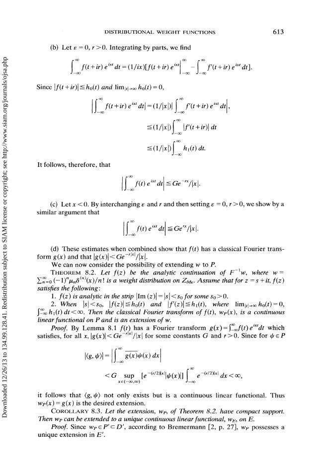
(b) Let e 0, r > 0. Integrating by parts, we find

ixtf(t + ir) e ixt dt (1/ix)[f(t + ir) e ixt f’(t + ir) e dt].

Since If(t + ir)[ -< ho(t) and limltl_ ho(t) 0,

f_ f(t+ir)eiXtdtl=(1/Ixl)[f f’(t+ir) eiXtdt],<--(1/IxlI [f’(t+ir)ldt

--< (1/I/I)f hi(t) dt.

It follows, therefore, that

f(t) e at <= Ge [x I.

(c) Let x < 0. By interchanging e and r and then setting e 0, r > 0, we show by asimilar argument that

(d) These estimates when combined show that f(t) has a classical Fourier trans-form g(x) and that [g(x) < Ge-rlxl/{x{.

We can now consider the possibility of extending w to P.THEOREM 8.2. Let f(z) be the analytic continuation of F-lw, where w

,=o (-1)lx,6(n)(x)/n! is a weight distribution on Zt. Assume that ]:or z s + it, f(z)satisfies the following:

1. f(z) is analytic in the strip [Im (z)[ Is I< So for some So > O.2. When ]s]<s0, If(z)l<-ho(t)and ]f’(z)l<=ha(t), where limltl_,ho(t)=O,- ha(t)dt <. Then the classical Fourier transform of f(t), we(x), is a continuous

linear functional on P and is an extension of w.

Proof. By Lemma 8.1 [(t) has a Fourier transform g(x)=_f(t)eiXtdt whichsatisfies, for all x, Ig(x)[< Ge-rlxl/Ixl for some constants G and r >0. Since for q P

<G sup [e-(r/=)lxllO(x)l]I_ exe(-oo,oo)

-(r/2)lXl dx < 00,

it follows that (g, 4) not only exists but is a continuous linear functional. Thuswe(x) g(x) is the desired extension.

COROLLARY 8.3. Let the extension, we, of Theorem 8.2. have compact support.Then we can be extended to a unique continuous linear functional, wE, on E.

Proof. Since we p’c D’, according to Bremermann [2, p. 27], we possesses aunique extension in E’.

Dow

nloa

ded

12/2

6/13

to 1

34.9

9.12

8.41

. Red

istr

ibut

ion

subj

ect t

o SI

AM

lice

nse

or c

opyr

ight

; see

http

://w

ww

.sia

m.o

rg/jo

urna

ls/o

jsa.

php


III. REGULARIZATIONS

9. An example. We have just seen how w can be extended when the analyticcontinuation, f, of F-lw has a classical Fourier transform. In what follows we shalldevote our attention to the problem of extending w when a classical Fourier transformdoes not exist.

As an illustration of what can occur consider the case of the generalized LaguerrefL-3/2polynomials In=0. In this case

w(x) ,=0E (-1)nr(_)nand

1 F(n-1/2)(_it),"F-lw(t).=0 F(-1/2)n.

It is easy to see that the analytic continuation of F-lw is (1/(2r))(l+it) 1/2, whichdoes not have a classical Fourier transform.

It does, however, have a derivative, if(t)= [i/(4r)](1 + it) -1/2, which is classicallytransformable"

Further, since

ix-/2 e-Xg(x)=F[f’(t)]= F(_21_) x >0,

0, x<_-0.

If ], F[4) ]) (-ixF[f], F[])

with the extension we equal to Fir], we see that Wp and g(x)/(ix) should represent thesame linear functional. But

1/2x e

Wp(X) g(x)/ix F(-1/2)O,

x>O,

x=<0

does not generate a continuous linear functional even on Z due to the singularity atx=0.

The difficulty exhibited above can be circumvented by a process known asregularization (see [3, pp. 45-81]), and it is this procedure which (still) generatescontinuous extensions of w to P or E.

A close examination of regularization follows. Let us say in closing this sectionthat the regularization of our example leads to the functional Wp generated by

(Wp, )= (I/F(--1/2)) f x-3/2(e-X(x)--(O)) dx,3o

or we e-Xx-3/z/F(-1/2), where

(X3/2, O)= fO X--3/2([I(X)--II(O)) dx.

10. Regularizations. For the moment let us consider the regularization of h(x)which has a singularity only at 0. We assume that h(x) is integrable over everybounded region of E’ not containing 0 either in its interior or on its boundary. A

Dow

nloa

ded

12/2

6/13

to 1

34.9

9.12

8.41

. Red

istr

ibut

ion

subj

ect t

o SI

AM

lice

nse

or c

opyr

ight

; see

http

://w

ww

.sia

m.o

rg/jo

urna

ls/o

jsa.

php


regularization of h(x) is a continuous linear functional which coincides with h(x)except at 0. That is, for every qt in the test space which vanishes in a neighborhood of0, the functional has the same value as _-(x)d(x) dx.

We quote the following two theorems from [3, p. 11].hTHEOREM 10.1 If there exists an m > 0 such that x (x is locally integrable, then

h (x) can be regularized.THEOREM 10.2. Any two regularizations of h (x differ by a functional concentrated

at O.If the regularization of h(x) also preserves the operations of addition, multipli-

cation by an appropriate function and differentiation, then the regularization is calledcanonical. Following [3] we write h =CRh(x) to denote that h is the canonicalregularization of h (x).

Finally we shall restrict our attention to those functions which can be written as

h(x)-_,pi(x)qi(x)

x -where each pi is infinitely differentiable, and each q is one of the functions x/, andx Then

CRh (x E pi (x)CRq (x ).

We remark that if h(x) has singularities of the kind mentioned above at morethan one point, say at XoXl’"x, and if y,.-., y are chosen so x0ylx y x, Y0 -, Y/ , and

h(x ), yi-l x yi,hi (x O, otherwise,

then h(x) can be decomposed into the sum hi(x), and each term can be handledseparately. This situation arises in a discussion of Jacobi polynomials, where sin-gularities occur at +/-1. For our purposes here we shall restrict our attention tosingularities at 0 only.

11. Regularized extensions. We assume that f(z) is the analytic continuation ofF-w and that f(m)(z), Z=t+is, is analytic withwhen Isl<so, where limltt_, h0(t) 0 andY h(t)dt.

THEOREM 11.1. Let g(x) denote the classical Fourier transform of fm)(t). Assumethat g(x)/(-ix) has a canonical regularization h(x). Then there exist constants Ck,

(kk=O,"" m-l, such that Wp(X)--h(x)+_Ck )(x) is a continuous linearextension of w to P.

Proof. The constraints on f guarantee that

_g(x)(x)dx is continuous on P.

This, in turn, insures that the canonical regularization of g(x)/(-ix) will be con-tinuous and linear on P.

Now wp=Ff is an extension of w. We claim there exist constants ck, k0,. ., m- 1, such that

m--1

6kWp(X) h (x) + Z Ck (X).k=O

Since h is continuous and linear on P, so will we be. Thus we is an extension of w to P.To see that in fact

m-1

Wp(X) Ff(x) h(x) + Z Ck 6(k(x),k=O

Dow

nloa

ded

12/2

6/13

to 1

34.9

9.12

8.41

. Red

istr

ibut

ion

subj

ect t

o SI

AM

lice

nse

or c

opyr

ight

; see

http

://w

ww

.sia

m.o

rg/jo

urna

ls/o

jsa.

php


we proceed as follows.(a) Let y(t)=F-lh(t). Then

2r(y(m), (t)) (Fy(m), F) ((-ix)mh, Fck).

Since (-ix) is infinitely differentiable,

(-ix)mh(x) (-ix)mCR[g(x)/(-ix)m]

CR[(-ix)mg(x)/(-ix) g(x).

Thus

2r(Ym), 4 {g, F 2r(fm), d 5.That is, Y

m) f{m).(b) Since every distribution in D’ has antiderivatives of mth order, we conclude

f(t) T(t) +1 (it)"k=O

Taking Fourier transforms, we find

Wp(X)= h(x)+ E Ck 8(k)(x).k=0

COROLLARY 11.2. e coecients Ck, k O, 1," , m 1, are given by

(-)[c -(, x )].

Praaf. Since (, x) , k 0,. and ()(x), x) (-1)k B,

=(,x)=(,x)+ E c(6")(x),x)k=0

=(h,x)+(-1)kc.COROLLARY 11.3. Let the extensian af earem 11.1 have campact suppart.

en can be extended ta a unique cantinuau8 linear functianal, , an E.

IV. ORTHOGONAL POLYNOMIALS

12. General orlhoonal olynomials. Let us consider the polynomials p(x)

1p.(x)

An-

defined by po 1,

n 1, 2,. ,where

/Xo /x

2n-1

1 x x

lff2n

n=0,1,...

Dow

nloa

ded

12/2

6/13

to 1

34.9

9.12

8.41

. Red

istr

ibut

ion

subj

ect t

o SI

AM

lice

nse

or c

opyr

ight

; see

http

://w

ww

.sia

m.o

rg/jo

urna

ls/o

jsa.

php


We assume that the distribution w has been extended to we, which is continuous on P.THEOREM t2.1. The collection {p,(x)}=0 is mutually orthogonal with respect to

we. That is, if rn n, (we, p,,p,) O.Proof. We note that if k < n, then

/Xo /

1 /x jtZ2 jtZn+lO,

k k+l k+n

since the last row will be identical with one above. Thus, when m < n, if p,(x)=kY.k=O CkX then

(Wp, PmPn)= Ck(Wp, xkp.)=.0.

THEOREM 12.2. (Wp, p2,,)= A,/A,_I O.Proof. (Wp, pZ,)=(Wp, X"p,), which, by observation of the formula above, is

A./A.-1.The precise connection between Wp and the classical weight functions follows.

13. The classical orthogonal polynomials.A. The Legendre polynomials. The moments for the Legendre polynomials are

/-/,2. 2/(2n + 1),/x2,+1 0. Thus

and

2(2n)(X)w ,0 (2n + 1)!’

This is a power series representation for

1 (it)2"

rr.=o(2n+l)!"

(e ite -it) [sin t]

f(t)(2rrit) (rrt)

This function has a classical Fourier transform

1,w (x)

0, Ix[> a.

B. The Laguerre polynomials. The moments for the Laguerre polynomials are/z. n !. Thus

w Z (-1)"n=0

and

F-lw . (-it)"/(27r).n=0

Dow

nloa

ded

12/2

6/13

to 1

34.9

9.12

8.41

. Red

istr

ibut

ion

subj

ect t

o SI

AM

lice

nse

or c

opyr

ight

; see

http

://w

ww

.sia

m.o

rg/jo

urna

ls/o

jsa.

php


This power series representation converges when It[ < 1 to (1/27r)(1 + it)-1. Thus theanalytic continuation of F-iw is

1(f(z)27r

1 + iz

We see with So=1/2, ho(t) (1/(27r))(1/(4 + t2))-1/2, hi(t) (1/(2r))(1/(4 + t2))-1, thatlimltl_ho(t)=O and that oo hi(t)dt <oo. Thus we=Ff extends w to P. Cauchy’sresidue then establishes that

e x>0,Wp

O, X < O.

C. The I-lermite polynomials. The moments for the Hermite polynomials are

tx2, =’(2n)!/(4nn!), L62n+l 0. Thus

w=n=o 4nn

and

F-lw=(2v)-i Z (-t2/4)".n=O n!

This is the power series representation for

f(z) (2x)-1 --z2/4e

--t2/4With So 1, ho(t)=e -t2/4, hl(t)=[It[/2]e we satisfy the conditions to extend w,and

we FZ(x e -x2, -oo<x <

14. Generalized Laguerre polynomials. H. L. Krall [4] has shown that thedifferential equation

(/22X 2 + 121X + 120)Pn + (l lx + lO)Pn (111n + 122n (n 1))pn

has a polynomial solution p,(x) of degree n for each n 0, 1,..., if and only if themoments {xi}=o satisfy An 0 and

lllt-6n +/10/-6n--1 +(n 1)[/22n +/21/,n-1 + 120t-6n--2] O,

n=1,2,-...For the Laguerre equation

xL(,,)"-[x -a 1]L()’+nnL()=. 0the recurrence relation above is/x, --[n + a]rt-1. Consequently,

THEOREM 14.1. Let Ixo 1. Then when a # 1, -2, ,r(n + a + 1)r(a + 1)

Note that these moments have been calculated by a technique not dependent onthe existence of a weight function. Further when a is a negative integer -no, allmoments x, 0 when n > no. In this case the formula for pn defines polynomials onlyup to degree no. This degenerate case will not be considered.

Dow

nloa

ded

12/2

6/13

to 1

34.9

9.12

8.41

. Red

istr

ibut

ion

subj

ect t

o SI

AM

lice

nse

or c

opyr

ight

; see

http

://w

ww

.sia

m.o

rg/jo

urna

ls/o

jsa.

php


Note further that the moments are not all positive when a <-1. If j 1 < c <-j, the first j moments alternate in sign. The remaining moments retain the same signas/-]--1.

Inserting the moments into the formula for w, we findTHEOREM 14.2. For the Laguerre polynomials {L(hln=O

(_1),r(n +a + 1) 6(">(x)

and

F-lw(t) (1/(2rr))(1 + it)--1.Whena> 1, F-1w can easily be inverted by tables [6]"THEOREM 14.3. When a > 1,

Hence

we(x) F(c + 1)’x _-> 0,

O, x<O.

n =0, 1, ,and

F(n + ce + 1) 1Io ,,+,/’= F(ce+l) -F(ce-+-l) x e dx,

(we, L)()) 1 Io L()L(2)(x)x e-x dx,r( + 1)

_(0 when m n,

!F(n+a+l)whenm=n.

r(c + 1)

A suitable weight function can also be found when a <- 1 and a is not a negativeinteger. Although F-lw cannot be directly inverted, a suitable derivative can be.

Let j 1 < a <-j, and replace (1 + it) by z. Then

F-lwp(z)= z--l/(27r).When z =0, F-lwp =0. Likewise when 0=<m <],

(F-’wp)(m(z)=(-1)m(a + 1) (a +m)z--m-/(27r),and (F-wp)(mlz=o= O. Finally,

(F-lwe) (-1)(c + 1)... (c +j)z--J-1/(27r)is the first derivative to become infinite at z 0, and is also the first to have a classicalFourier transform. Its transform is [6]

(_ 1)x +

w(x) F(c + 1)x _->0,

0, x<0.

Hence

(-1) f x+ e-X(F-we)(J(t)27rF(a + 1)

e -itx dx(-1)i fo x’+

27rF(c + 1)e dx.

Dow

nloa

ded

12/2

6/13

to 1

34.9

9.12

8.41

. Red

istr

ibut

ion

subj

ect t

o SI

AM

lice

nse

or c

opyr

ight

; see

http

://w

ww

.sia

m.o

rg/jo

urna

ls/o

jsa.

php


If integration in z is performed j times with limits from 0 to z, we find

F-1 (z)2rrF(a + 1) k=0

Wp X e _, (--1)kxkzk/k dx

=2F(+l) x e e -=o (-1)x(l+it)/k dx.

If the last term is expanded in powers of -it, and the summation indices are reversed,this becomes

1x -. (-1)x

dx.F-we(t)=2F(a + 1)e e (-1) (-it)

Since (-it)= (e-")( evaluated at x 0, this suggests that the regularization of w is

1 _xo (-1)xe (x)- l(k (-1)(’)(0) dx.(w, )=

F(a + 1)x

This agrees with [3]. An evaluation of (w, x) indeed verifies that

F(n +a +1)(w,x")

F(a + )

n =0, 1,.... ThusTHEOREM 14.4. Let j 1 <a <-]. en the Laguerre polynomials {L)(x)}_o

are mutually orthogonal with respect to the linear functional Wn defined by

1 _xo (-1)xe (x)- l!(k--i} (-1)0()(0) dx.(w, )=

r( + )x

Direct computation of the norms (squared) of L(2 ), (w,t(n)2) is extremelyawkward. By using the recurrence relation [7], however, they quickly follow:

THEOREM 14.5. For all a -1,-2,. ,(we, L) n !F(n + a + 1)

F(a + 1)

n=0, 1,....Proof. We multiply the relation

,/- (c)l,()+(x a-2n-1)L)+n(n+a,n_l=Oby L()

+1 and apply Wp to see

(a)2\ (a)l(a)(we, L,+i/+(Wn, xL )=0+

If n is replaced by n + 1 in the recurrence relation, it becomes

,+2+(x-a-2n-3atn++(n + 1)(n +a + 1)L) 0.

If this is multiplied by L) and we is applied, then we have

(Wn, xL+L +(n + 1)(n +a + 1)(wn, L2)=O.Thus

(a)2\(Wp, L2) n (n + a )(Wp, L,-I/.

The result follows by induction.

Dow

nloa

ded

12/2

6/13

to 1

34.9

9.12

8.41

. Red

istr

ibut

ion

subj

ect t

o SI

AM

lice

nse

or c

opyr

ight

; see

http

://w

ww

.sia

m.o

rg/jo

urna

ls/o

jsa.

php


The values n!F(n +a+ 1)/F(a + 1), of course, coincide with previous resultswhen a >- 1. When a <- 1, however, they are new. They oscillate in sign just as dothe moments

15. The Jacobi polynomials. The Jacobi polynomials can also be made ortho-gonal in an extended sense, although a number of modifications in technique arerequired.

First the formulas of H. L. Krall [4] exhibited at the beginning of 14 are asfollows. If the differential equation for the Jacobi polynomials2 {Pn}n=O is

(1 -x2)p’. +[(u -v)-(u + v)x]P’. + n(u + v + n 1)P. 0,

the moment recurrence relation is

[U +V + n- 1]/Xn--[U + ]/Xn-1--[/- 1]/x,-2 0.

This is easily solved only in such simple cases as u 0, v 0 or u =-v, which aredegenerate. Further, a direct computation of/xn through the formula

Xn(1--X)V-l(l +X)u-1 dx

is available only when u, v > 0. Consequently a direct qomputation of the momentsdoes not seem reasonable.

Instead we follow a procedure developed by R. D. Morton. In the relations of H.L. Krall [4] replace x by y x- Xo. Then the differential equation is transformed into

[122y 2 + (2/22X0 + 121)Y + (122X02 + 121X0 + 120)]pn + [/llY + (/11Xo + llo)]Pn

n[(111-lzz)+lzzn]p,,and the recurrence relation becomes

(nl22 + 111 122)/x, (Xo) + ([111 + (n 1)122Xo + n121 + 1o- I21)/x,-a (Xo)

+(/ 1)(/22Xg -k- 121X0 +/20)/x,,-2(Xo) 0,

where/x, (Xo) is the nth moment about xo.If xo is chosen so that 122x + 121xo +/20 0, then the recurrence relation becomes

"two term", and is easily solved.For the Jacobi polynomials the recurrence relation is simplified when -xg + 1 0,

or Xo + 1.THEOREM 15.1. Let IXo 1. Then the Jacobi moments about 1,/x,(1), are

.()(u+v),

n O, 1, where (a), a(a + l) (a + n -1).Proof. The recurrence relation with Xo 1 is

/x, (1)(u +v + n- 1) +/x,_l(1)2(v + n- 1)= 0,

which is solvbd by induction.

Traditionally the Jacobi polynomials are indicated by {Pn’ }n=o. For notational purposes we set1,/3 u and suppress c and/3.

Dow

nloa

ded

12/2

6/13

to 1

34.9

9.12

8.41

. Red

istr

ibut

ion

subj

ect t

o SI

AM

lice

nse

or c

opyr

ight

; see

http

://w

ww

.sia

m.o

rg/jo

urna

ls/o

jsa.

php


THEORFM 15.2. Let tXo 1. Then the Jacobi moments about -1,/xn (-1), are

(U + t)n’

n=0,1,....As can be seen by inspection, there are three degenerate cases.1. If v -N, then /XN+I(1) 0, and hence /x (1) 0 for all n > N. Only poly-

nomials up to degree N exist.2. If u -N, then /XN+I(-- 1) 0, and hence ,, (- 1) 0 for all n > N. Only

polynomials up to degree N exist.3. If u +v =-N, then either about 1 or -1 /xN+I is undefined, as are the Jacobi

polynomials.W.e assume, therefore, that u, v, u + v are not 0 or negative integers.THEOREM 15.3. Let txo 1. Then the Jacobi moments about O, txn (0), are

tx.(0)= J (-1)2(v)_ J(-1) (u).

=0 (u + v) .=Z0 (u + v)

,(0) (w, x") (w, [(x 1)+

= j ;=o jre(l).

Substitution yields the first expression. A similar expansion about -1 yields thesecond.

Since /x0 1, tx(1)=(u-v)/(u +v) in both expressions above, the recurrencerelation verifies their equivalence for all n,

If we temporarily assume that u and v are complex with Re u > 0, Re v > 0, thenthe function

WE(X)0,

has as its inverse Fourier transform [6]

-l__<x<__l

]x] > 1,

itF-lwE(t)=e 1Fl(U, u +19,-2it)/(27r).

If this is expanded in a power series in (-it), then

w(t) =o (u + v)y - !2--’

Z I,(O)(-it)"/n!,

where the moment formula for tz, (0) using an expansion about -1 has been inserted.A comparison shows this formula agrees with the distributional inverse Fouriertransform F-w.

Dow

nloa

ded

12/2

6/13

to 1

34.9

9.12

8.41

. Red

istr

ibut

ion

subj

ect t

o SI

AM

lice

nse

or c

opyr

ight

; see

http

://w

ww

.sia

m.o

rg/jo

urna

ls/o

jsa.

php


Likewise, since

1Fl(a, b, z)= eZIFa(b-a, b, -z),

b : 0,-1,. , (see Rainville [7, p. 125]),

F-lwe(t) e-itaFa(v, u + v, 2it)/(27r),

.o ] - -T- i; _! n !2rr’

1Z ,(O)(-it)"/n,

where the moment formula for >, (0) using an expansion about 1 has been inserted. Acomparison again shows that F-1 w.we agrees with F-

Rather than retrace the tedious calculations through a number of steps to find thevarious equivalent formulas when Re u < 0, Re v < 0 and u, v, u + v 0, -1, ,instead we use the principle of analytic continuation in u and v to achieve the results.We note that for Re u > 0 and Re v > 0, the following hold [7]:

Distributional formula.F(u +v) ] )u_,0(we, O)=r(u)r(v)2u+_ (1-x)-(l+x (x) dx.

Inverse Fourier transform.

F-lwe(t) eitlFl(U, u -I V,-2it)/(27r) e-itFl(V, u + v, 2it)/(27r).

Orthogonality.

<we, P,Pm>= O, n m.

Norm squared.

<wF, P> F(u + v)F(u + n)F(v + n)F(u)F(v)F(u +v + n 1)(u +v + 2n 1)n!’

THEOREM 15.4. Let -M + 1 > u > -M, -N + 1 > v > -N, M, N> O. Then thefollowing hold"

Distributional formula.

(w,4,}= r(u)r(v)2u+_l x (-x)-’ (l+x 6(x)

N-I[(I+x)U-1 )]q) }Z (x (-1)(1-x) ax=o ] =

0 { )v_lo M-l[(l__x)V-lO(x)](k) }+ (+x)-’ (1-x (x)- E (l+x) dx-1 =o k x=-

+ N-l[(l+x)U-IE (X)]0")=0 j!

M-1 [(l--x)v-1+ Y

q’(x)](k=O k!

(-1);x=l (V "+’j)

=_l/(U "]" k)].

Dow

nloa

ded

12/2

6/13

to 1

34.9

9.12

8.41

. Red

istr

ibut

ion

subj

ect t

o SI

AM

lice

nse

or c

opyr

ight

; see

http

://w

ww

.sia

m.o

rg/jo

urna

ls/o

jsa.

php


Inverse Fourier transform.

F-lwE(t) eitlFl(U, u + v,-2it)/(27r) e-itlFl(u, u + v, 2it)/(2rc).

Orthogonality.

(wE, P,,P,,,) O, n m.

Norm squared.

(wE, p2)=F(u + v)F(u + n)F(v + n)

F(u)F(v)F(u +v + n 1)(u +v + 2n 1)n !"

Proof. It is clear that in each of these formulas the right sides are the analyticcontinuations of the right sides when Re u > 0, Re v > 0. The distributional formulas

--ixt 2for the application of wE to 0, e /zvr, PnP, or Pn are the canonical regularizationsof the application of the analytic continuation of wE, and in fact (see [3, p. 66]) theresults are the analytic continuations of the integrals which result when Re u >0,Re v > 0. As analytic continuations they must still agree.

16. The Bessel polynomials. Unfortunately the Bessel polynomials fail to yieldcompletely to the techniques of this paper. The moments for the Bessel polynomialsare/xn (-2)n+l/(n + 1)!. Thus

2n+1 (n)(x)w(x) -.=oy n!(n + 1).

and

F-lw(t)= -1 2"+1(it)"27r ,=0 n !(n + 1)!’

which is the power series representation for

-1 I((8it) 1/2)f(t) 1/2

7r (S/t)

Since If(t)l-(a/,/-)exp [21tl/]/(sZltl)/4 for large Itl, an extension of w beyond Sstill remains to be found.

Various tables (e.g. [8, #656.4]) show that F-w corresponds to (1/-n’)e -2/x.Direct calculation using the Bessel polynomial differential equation,

2x y, +[2x + 2]y, n(n + 1)y,,

however, shows this is incorrect. The authors have devoted a great deal of time toextending w but are still left with the formula

Wp =FfTr-1 I((8it)1/2)](Sit)l2

which has defied evaluation.It is possible to give a direct proof of orthogonality of the Bessel polynomials

without resorting to the moment formula for pn. All that is required is the existence ofa weight function w or measure , which gives the moments through the formulas/x, =(w,x), which certainly holds, or through /x, =x d,. Such a measure , ofbounded variation on [0, ) is guaranteed by Boas [1].

Dow

nloa

ded

12/2

6/13

to 1

34.9

9.12

8.41

. Red

istr

ibut

ion

subj

ect t

o SI

AM

lice

nse

or c

opyr

ight

; see

http

://w

ww

.sia

m.o

rg/jo

urna

ls/o

jsa.

php


The classical Bessel polynomials are given by the formula

yn(x) k=O’ (n k)k.n O, 1,. .

Since the highest order coefficient is (2n)!/(2"n !), y, [(2n)!/(2"n !)]p,.Let us define

A Z (-1)k (n+k)!k=O (m + k + 1)!"

LEMMA 16.1 Let 0 < m < n. Then A O.Proof. Consider

n+k

Then

k=0 (m +k + 1)!m+k+l

X

and f("-m-1)(1)=A,.Since f(n-m-1)(1)--O when 0--<m <n, so is A.THEOREM 16.2 The Bessel polynomials are mutually orthogonal with respect to w

or with respect to an appropriate measure u which generates the moments I,-(-1)"+l/(n+1)!,n=0,1,....

Proof. If 0=m <n,

Xj+k(n +k)’(m +])’(w,

(w, yy,,) k=Oi=O/" (n-k)!k!(n-j)!j!2i+k

(n +k)!(m +j)!(-1)i+k+12k=O i=oZ (n k)’k. --(.j);- -7t-1)’.

=2 ( (m+])’(-1)i+’].=o (m -y)!j!n a7 =o.

The norms (squared) can also be readily calculated. Define

B,= 2 o (n +k)!(n +])!(-1)+k+

k=Oi= (n-k)!k!(m-j)!j!(j+k + l)!"

LEMMA 16.3. If m =n >--1, then B,=(-1)"+2/(2n + 1).Proof. Again consider

f(x)=xn(l_x).= (_l)k(n) n+k

k=O kx

Let

F(y) f(x) dx (-1)k y.+k+ /(n + k + 1).

Then F(1) A,. But if integration by parts is performed n times,

F(1)=[(n!)2/(2n)!] (1-x dx =(n!)2/(2n + 1)!.

Dow

nloa

ded

12/2

6/13

to 1

34.9

9.12

8.41

. Red

istr

ibut

ion

subj

ect t

o SI

AM

lice

nse

or c

opyr

ight

; see

http

://w

ww

.sia

m.o

rg/jo

urna

ls/o

jsa.

php


Thus A, (n !)2/(2n + 1)! and

B, 2[(2n)!!(-1)n+l/(n !)2]Ann (--1)n+12/(2n + 1).

We have only to note that either (w, y,,2) or y2 dv equal B to concludeTHEOREM 16.4. The Bessel polynomials satisfy

or (-1)"2/(2n + 1).2y. dv

This is in agreement with the calculation done by H. L. Krall and O. Frink [5]using a different method.

REFERENCES

[1] R. P. BOAS, JR., The Stielt]es moment problem ]:or functions o]" bounded variation, Bull. Amer. Math.Soc., 45 (1939), pp. 399-404.

[2] H. BREMERMANN, Distributions, Complex Variables, and Fourier Transforms, Addison-Wesley,Reading, MA, 1965.

[3] I. M. GEL’FAND AND G. E. SHILOV, Generalized Functions, vol. I, Academic Press, New York, 1964.[4] H. L. KRALL, Certain differential equations ]’or Tchebycheffpolynomials, Duke Math. J., 4 (1938), pp.

705-718.[5] H. L. KRALL AND O. FRINK, A new class of orthogonal polynomials: The Bessel polynomials, Trans.

Amer. Math. Soc., 65 (1949), pp. 100-115.[6] F. OBERHETrINGER, Tabellen zur Fourier Tranfformen, Springer-Verlag, Berlin, 1957.[7] E. O. RAINVILLE, Special Functions, Macmillan, New York, 1960.[8] B. W. Roos, Analytic Functions and Distributions in Physics and Engineering, Joln Wiley, New York,

1969.

Dow

nloa

ded

12/2

6/13

to 1

34.9

9.12

8.41

. Red

istr

ibut

ion

subj

ect t

o SI

AM

lice

nse

or c

opyr

ight

; see

http

://w

ww

.sia

m.o

rg/jo

urna

ls/o

jsa.

php

Documents

Distributional Weight Functions for Orthogonal Polynomials