Numerical Methods I Orthogonal Polynomials - NYU …donev/Teaching/NMI-Fall2014/Lecture9.handout.pdfNumerical Methods I Orthogonal Polynomials Aleksandar Donev Courant Institute, NYU1

Numerical Methods IOrthogonal Polynomials

Aleksandar DonevCourant Institute, NYU1

[email protected]

1Course G63.2010.001 / G22.2420-001, Fall 2010

Nov. 4th and 11th, 2010

A. Donev (Courant Institute) Lecture VIII 11/04/2010 1 / 40

Outline

1 Function spaces

2 Orthogonal Polynomials on [−1, 1]

3 Spectral Approximation

4 Fourier Orthogonal Trigonometric Polynomials

5 Conclusions


Final Project Presentations

The final presentations will take place on the following three dates(tentative list!):

1 Thursday Dec. 16th 5-7pm (there will be no class on LegislativeDay, Tuesday Dec. 14th)

2 Tuesday Dec. 21st 5-7pm

3 Thursday Dec. 23rd 4-7pm (note the earlier start time!)

There will be no homework this week: Start thinking about the projectuntil next week’s homework.


Lagrange basis on 10 nodes

0 0.1 0.2 0.3 0.4 0.5 0.6 0.7 0.8 0.9 1−7

−6

−5

−4

−3

−2

−1

0

1

2A few Lagrange basis functions for 10 nodes

φ5

φ1

φ3


Runge’s phenomenon f (x) = (1 + x2)−1

−5 −4 −3 −2 −1 0 1 2 3 4 5−5

−4

−3

−2

−1

0

1Runges phenomenon for 10 nodes

x

y


Function spaces

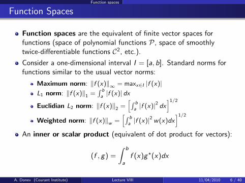
Function Spaces

Function spaces are the equivalent of finite vector spaces forfunctions (space of polynomial functions P, space of smoothlytwice-differentiable functions C2, etc.).

Consider a one-dimensional interval I = [a, b]. Standard norms forfunctions similar to the usual vector norms:

Maximum norm: ‖f (x)‖∞ = maxx∈I |f (x)|L1 norm: ‖f (x)‖1 =

∫ b

a|f (x)| dx

Euclidian L2 norm: ‖f (x)‖2 =[∫ b

a|f (x)|2 dx

]1/2Weighted norm: ‖f (x)‖w =

[∫ b

a|f (x)|2 w(x)dx

]1/2An inner or scalar product (equivalent of dot product for vectors):

(f , g) =

∫ b

af (x)g?(x)dx


Function spaces

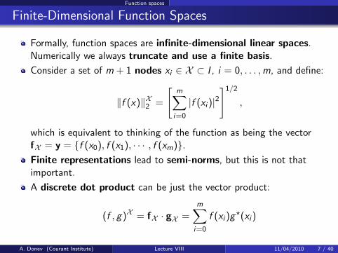
Finite-Dimensional Function Spaces

Formally, function spaces are infinite-dimensional linear spaces.Numerically we always truncate and use a finite basis.

Consider a set of m + 1 nodes xi ∈ X ⊂ I , i = 0, . . . ,m, and define:

‖f (x)‖X2 =

[m∑i=0

|f (xi )|2]1/2

,

which is equivalent to thinking of the function as being the vectorfX = y = {f (x0), f (x1), · · · , f (xm)}.Finite representations lead to semi-norms, but this is not thatimportant.

A discrete dot product can be just the vector product:

(f , g)X = fX · gX =m∑i=0

f (xi )g?(xi )


Function spaces

Function Space Basis

Think of a function as a vector of coefficients in terms of a set of nbasis functions:

{φ0(x), φ1(x), . . . , φn(x)} ,

for example, the monomial basis φk(x) = xk for polynomials.

A finite-dimensional approximation to a given function f (x):

f̃ (x) =n∑

i=1

ciφi (x)

Least-squares approximation for m > n (usually m� n):

c? = arg minc

∥∥∥f (x)− f̃ (x)∥∥∥2,

which gives the orthogonal projection of f (x) onto thefinite-dimensional basis.


Function spaces

Least-Squares Approximation

Discrete case: Think of fitting a straight line or quadratic throughexperimental data points.

The function becomes the vector y = fX , and the approximation is

yi =n∑

j=1

cjφj(xi ) ⇒ y = Φc,

Φij = φj(xi ).

This means that finding the approximation consists of solving anoverdetermined linear system

Φc = y

Note that for m = n this is equivalent to interpolation. MATLAB’spolyfit works for m ≥ n.


Function spaces

Normal Equations

Recall that one way to solve this is via the normal equations:

(Φ?Φ) c? = Φ?y

A basis set is an orthonormal basis if

(φi , φj) =m∑

k=0

φi (xk)φj(xk) = δij =

{1 if i = j

0 if i 6= j

Φ?Φ = I (unitary or orthogonal matrix) ⇒

c? = Φ?y ⇒ ci = φXi · fX =m∑

k=0

f (xk)φi (xk)


Orthogonal Polynomials on [−1, 1]

Orthogonal Polynomials

Consider a function on the interval I = [a, b].Any finite interval can be transformed to I = [−1, 1] by a simpletransformation.

Using a weight function w(x), define a function dot product as:

(f , g) =

∫ b

aw(x) [f (x)g(x)] dx

For different choices of the weight w(x), one can explicitly constructbasis of orthogonal polynomials where φk(x) is a polynomial ofdegree k (triangular basis):

(φi , φj) =

∫ b

aw(x) [φi (x)φj(x)] dx = δij ‖φi‖2 .



Legendre Polynomials

For equal weighting w(x) = 1, the resulting triangular family of ofpolynomials are called Legendre polynomials:

φ0(x) =1

φ1(x) =x

φ2(x) =1

2(3x2 − 1)

φ3(x) =1

2(5x3 − 3x)

φk+1(x) =2k + 1

k + 1xφk(x)− k

k + 1φk−1(x) =

1

2nn!

dn

dxn

[(x2 − 1

)n]These are orthogonal on I = [−1, 1]:∫ −1

−1φi (x)φj(x)dx = δij ·

2

2i + 1.



Interpolation using Orthogonal Polynomials

Let’s look at the interpolating polynomial φ(x) of a function f (x)on a set of m + 1 nodes {x0, . . . , xm} ∈ I , expressed in an orthogonalbasis:

φ(x) =m∑i=0

aiφi (x)

Due to orthogonality, taking a dot product with φj (weakformulation):

(φ, φj) =m∑i=0

ai (φi , φj) =m∑i=0

aiδij ‖φi‖2 = aj ‖φj‖2

This is equivalent to normal equations if we use the right dotproduct:

(Φ?Φ)ij = (φi , φj) = δij ‖φi‖2 and Φ?y = (φ, φj)



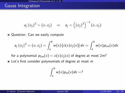
Gauss Integration

aj ‖φj‖2 = (φ, φj) ⇒ aj =(‖φj‖2

)−1(φ, φj)

Question: Can we easily compute

aj ‖φj‖2 = (φ, φj) =

∫ b

aw(x) [φ(x)φj(x)] dx =

∫ b

aw(x)p2m(x)dx

for a polynomial p2m(x) = φ(x)φj(x) of degree at most 2m?

Let’s first consider polynomials of degree at most m∫ b

aw(x)pm(x)dx =?



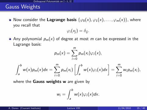
Gauss Weights

Now consider the Lagrange basis {ϕ0(x), ϕ1(x), . . . , ϕm(x)}, whereyou recall that

ϕi (xj) = δij .

Any polynomial pm(x) of degree at most m can be expressed in theLagrange basis:

pm(x) =m∑i=0

pm(xi )ϕi (x),

∫ b

aw(x)pm(x)dx =

m∑i=0

pm(xi )

[∫ b

aw(x)ϕi (x)dx

]=

m∑i=0

wipm(xi ),

where the Gauss weights w are given by

wi =

∫ b

aw(x)ϕi (x)dx .



Back to Interpolation

For any polynomial p2m(x) there exists a polynomial quotient qm−1and a remainder rm such that:

p2m(x) = φm+1(x)qm−1(x) + rm(x)

∫ b

aw(x)p2m(x)dx =

∫ b

a[w(x)φm+1(x)qm−1(x) + w(x)rm(x)] dx

= (φm+1, qm−1) +

∫ b

aw(x)rm(x)dx

But, since φm+1(x) is orthogonal to any polynomial of degree at mostm, (φm+1, qm−1) = 0 and we thus get:∫ b

aw(x)p2m(x)dx =

m∑i=0

wi rm(xi )



Gauss nodes

Finally, if we choose the nodes to be zeros of φm+1(x), then

rm(xi ) = p2m(xi )− φm+1(xi )qm−1(xi ) = p2m(xi )

∫ b

aw(x)p2m(x)dx =

m∑i=0

wip2m(xi )

and thus we have found a way to quickly project any polynomialonto the basis of orthogonal polynomials:

(pm, φj) =m∑i=0

wipm(xi )φj(xi )

(φ, φj) =m∑i=0

wiφ(xi )φj(xi ) =m∑i=0

wi f (xi )φj(xi )



Gauss-Legendre polynomials

For any weighting function the polynomial φk(x) has k simple zerosall of which are in (−1, 1), called the (order k) Gauss nodes,φm+1(xi ) = 0.

The interpolating polynomial φ(xi ) = f (xi ) on the Gauss nodes is theGauss-Legendre interpolant φGL(x).

The orthogonality relation can be expressed as a sum instead ofintegral:

(φi , φj) =m∑i=0

wiφi (xi )φj(xi ) = δij ‖φi‖2

We can thus define a new weighted discrete dot product

f · g =m∑i=0

wi figi



Discrete Orthogonality of Polynomials

The orthogonal polynomial basis is discretely-orthogonal in the newdot product,

φi · φj = (φi , φj) = δij (φi · φi )

This means that the matrix in the normal equations is diagonal:

Φ?Φ = Diag{‖φ0‖2 , . . . , ‖φm‖2

}⇒ ai =

f · φi

φi · φi

.

The Gauss-Legendre interpolant is thus easy to compute:

φGL(x) =m∑i=0

f · φi

φi · φi

φi (x).


Spectral Approximation

Hilbert Space L2w

Consider the Hilbert space L2w of square-integrable functions on

[−1, 1]:

∀f ∈ L2w : (f , f ) = ‖f ‖2 =

∫ 1

−1w(x) [f (x)]2 dx <∞.

Legendre polynomials form a complete orthogonal basis for L2w :

∀f ∈ L2w : f (x) =

∞∑i=0

fiφi (x)

fi =(f , φi )

(φi , φi ).

The least-squares approximation of f is a spectral approximationand is obtained by simply truncating the infinite series:

φsp(x) =m∑i=0

fiφi (x).



Spectral approximation

Continuous (spectral approximation): φsp(x) =m∑i=0

(f , φi )

(φi , φi )φi (x).

Discrete (interpolating polynomial): φGL(x) =m∑i=0

f · φi

φi · φi

φi (x).

If we approximate the function dot-products with the discreteweighted products

(f , φi ) ≈m∑j=0

wj f (xj)φi (xj) = f · φi ,

we see that the Gauss-Legendre interpolant is a discrete spectralapproximation:

φGL(x) ≈ φsp(x).



Discrete spectral approximation

Using a spectral representation has many advantages for functionapproximation: stability, rapid convergence, easy to add morebasis functions.

The convergence, for sufficiently smooth (nice) functions, is morerapid than any power law

‖f (x)− φGL(x)‖ ≤ C

Nd

(d∑

k=0

∥∥∥f (k)∥∥∥2)1/2

,

where the multiplier is related to the Sobolev norm of f (x).

For f (x) ∈ C1, the convergence is also pointwise with similaraccuracy (Nd−1/2 in the denominator).

This so-called spectral accuracy (limited by smoothness only)cannot be achived by piecewise, i.e., local, approximations (limited byorder of local approximation).



Regular grids

a=2;f = @( x ) cos (2∗ exp ( a∗x ) ) ;

x f i n e=l i n s p a c e (−1 ,1 ,100) ;y f i n e=f ( x f i n e ) ;

% Equi−spaced nodes :n=10;x=l i n s p a c e (−1 ,1 ,n ) ;y=f ( x ) ;c=p o l y f i t ( x , y , n ) ;y i n t e r p=p o l y v a l ( c , x f i n e ) ;

% Gauss nodes :[ x ,w]=GLNodeWt(n ) ; % See webpage f o r codey=f ( x ) ;c=p o l y f i t ( x , y , n ) ;y i n t e r p=p o l y v a l ( c , x f i n e ) ;



Gauss-Legendre Interpolation

−1 −0.8 −0.6 −0.4 −0.2 0 0.2 0.4 0.6 0.8 1−5

−4

−3

−2

−1

0

1

2Function and approximations for n=10

Actual

Equi−spaced nodes

Standard approx

Gauss nodes

Spectral approx

−1 −0.8 −0.6 −0.4 −0.2 0 0.2 0.4 0.6 0.8 1−6

−5

−4

−3

−2

−1

0

1

2Error of interpolants/approximants for n=10

Standard approx

Spectral approx



Global polynomial interpolation error

−1 −0.8 −0.6 −0.4 −0.2 0 0.2 0.4 0.6 0.8 110

−16

10−14

10−12

10−10

10−8

10−6

10−4

10−2

100

Error for equispaced nodes for n=8,16,32,..128

−1 −0.8 −0.6 −0.4 −0.2 0 0.2 0.4 0.6 0.8 110

−16

10−14

10−12

10−10

10−8

10−6

10−4

10−2

100

Error for Gauss nodes for n=8,16,32,..128



Local polynomial interpolation error

−1 −0.8 −0.6 −0.4 −0.2 0 0.2 0.4 0.6 0.8 110

−8

10−7

10−6

10−5

10−4

10−3

10−2

10−1

100

101

Error for linear interpolant for n=8,16,32,..256

−1 −0.8 −0.6 −0.4 −0.2 0 0.2 0.4 0.6 0.8 110

−16

10−14

10−12

10−10

10−8

10−6

10−4

10−2

100

Error for cubic spline for n=8,16,32,..256


Fourier Orthogonal Trigonometric Polynomials

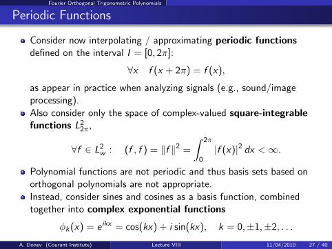
Periodic Functions

Consider now interpolating / approximating periodic functionsdefined on the interval I = [0, 2π]:

∀x f (x + 2π) = f (x),

as appear in practice when analyzing signals (e.g., sound/imageprocessing).

Also consider only the space of complex-valued square-integrablefunctions L2

2π,

∀f ∈ L2w : (f , f ) = ‖f ‖2 =

∫ 2π

0|f (x)|2 dx <∞.

Polynomial functions are not periodic and thus basis sets based onorthogonal polynomials are not appropriate.

Instead, consider sines and cosines as a basis function, combinedtogether into complex exponential functions

φk(x) = e ikx = cos(kx) + i sin(kx), k = 0,±1,±2, . . .



Fourier Basis

φk(x) = e ikx , k = 0,±1,±2, . . .

It is easy to see that these are orhogonal with respect to thecontinuous dot product

(φj , φk) =

∫ 2π

x=0φj(x)φ?k(x)dx =

∫ 2π

0exp [i(j − k)x ] dx = 2πδij

The complex exponentials can be shown to form a completetrigonometric polynomial basis for the space L2

2π, i.e.,

∀f ∈ L22π : f (x) =

∞∑k=−∞

f̂ke ikx ,

where the Fourier coefficients can be computed for any frequencyor wavenumber k using:

f̂k =(f , φk)

2π=

1

2π.

∫ 2π

0f (x)e−ikxdx .



Discrete Fourier Basis

For a general interval [0,X ] the discrete frequencies are

k =2π

Xκ κ = 0,±1,±2, . . .

For non-periodic functions one can take the limit X →∞ in whichcase we get continuous frequencies.

Now consider a discrete Fourier basis that only includes the first Nbasis functions, i.e.,{

k = −(N − 1)/2, . . . , 0, . . . , (N − 1)/2 if N is odd

k = −N/2, . . . , 0, . . . ,N/2− 1 if N is even,

and for simplicity we focus on N odd.

The least-squares spectral approximation for this basis is:

f (x) ≈ φ(x) =

(N−1)/2∑k=−(N−1)/2

f̂ke ikx .



Discrete Dot Product

Now also discretize the functions on a set of N equi-spaced nodes

xj = jh where h =2π

N

where j = N is the same node as j = 0 due to periodicity so we onlyconsider N instead of N + 1 nodes.

We also have the discrete dot product between two discretefunctions (vectors) f j = f (xj):

f · g = hN−1∑j=0

fig?i

The discrete Fourier basis is discretely orthogonal

φk · φk′ = 2πδk,k′



Proof of Discrete Orthogonality

The case k = k ′ is trivial, so focus on

φk · φk′ = 0 for k 6= k ′

∑j

exp (ikxj) exp(−ik ′xj

)=∑j

exp [i (∆k) xj ] =N−1∑j=0

[exp (ih (∆k))]j

where ∆k = k − k ′. This is a geometric series sum:

φk · φk′ =1− zN

1− z= 0 if k 6= k ′

since z = exp (ih (∆k)) 6= 1 andzN = exp (ihN (∆k)) = exp (2πi (∆k)) = 1.



Discrete Fourier Transform

The Fourier interpolating polynomial is thus easy to construct

φN(x) =

(N−1)/2∑k=−(N−1)/2

f̂(N)k e ikx

where the discrete Fourier coefficients are given by

f̂(N)k =

f · φk

2π=

1

N

N−1∑j=0

f (xj) exp (−ikxj)

Simplifying the notation and recalling xj = jh, we define the theDiscrete Fourier Transform (DFT):

f̂k =1

N

N−1∑j=0

fj exp

(−2πijk

N

)A. Donev (Courant Institute) Lecture VIII 11/04/2010 32 / 40


Fourier Spectral Approximation

Forward f → f̂ : f̂k =1

N

N−1∑j=0

fj exp

(−2πijk

N

)

Inverse f̂ → f : f (x) ≈ φ(x) =

(N−1)/2∑k=−(N−1)/2

f̂ke ikx

There is a very fast algorithm for performing the forward andbackward DFTs called the Fast Fourier Transform (FFT), whichwe will discuss next time.

The Fourier interpolating polynomial φ(x) has spectral accuracy,i.e., exponential in the number of nodes N

‖f (x)− φ(x)‖ ∼ e−N

for sufficiently smooth functions (sufficiently rapid decay of theFourier coefficients with k, e.g., f̂k ∼ e−|k|).



Discrete spectrum

The set of discrete Fourier coefficients f̂ is called the discretespectrum, and in particular,

Sk =∣∣∣f̂k ∣∣∣2 = f̂k f̂ ?k ,

is the power spectrum which measures the frequency content of asignal.

If f is real, then f̂ satisfies the conjugacy property

f̂−k = f̂ ?k ,

so that half of the spectrum is redundant and f̂0 is real.

For an even number of points N the largest frequency k = −N/2does not have a conjugate partner.



In MATLAB

The forward transform is performed by the function f̂ = fft(f ) andthe inverse by f = fft(f̂ ). Note that ifft(fft(f )) = f and f and f̂ maybe complex.

In MATLAB, and other software, the frequencies are not ordered inthe “normal” way −(N − 1)/2 to +(N − 1)/2, but rather, thenonnegative frequencies come first, then the positive ones, so the“funny” ordering is

0, 1, . . . , (N − 1)/2, −N − 1

2,−N − 1

2+ 1, . . . ,−1.

This is because such ordering (shift) makes the forward and inversetransforms symmetric.

The function fftshift can be used to order the frequencies in thenormal way, and ifftshift does the reverse:

f̂ = fftshift(fft(f )) (normal ordering).



FFT-based noise filtering (1)

Fs = 1000 ; % Sampl ing f r e qu enc ydt = 1/Fs ; % Sampl ing i n t e r v a lL = 1000 ; % Length o f s i g n a lt = ( 0 : L−1)∗dt ; % Time v e c t o rT=L∗ dt ; % Tota l t ime i n t e r v a l

% Sum of a 50 Hz s i n u s o i d and a 120 Hz s i n u s o i dx = 0.7∗ s i n (2∗ p i ∗50∗ t ) + s i n (2∗ p i ∗120∗ t ) ;y = x + 2∗ randn ( s i z e ( t ) ) ; % S i n u s o i d s p l u s n o i s e

f i g u r e ( 1 ) ; c l f ; p l o t ( t ( 1 : 1 0 0 ) , y ( 1 : 1 0 0 ) , ’ b−− ’ ) ; hold ont i t l e ( ’ S i g n a l Cor rupted wi th Zero−Mean Random Noi se ’ )x l a b e l ( ’ t ime ’ )




i f (0 )N=(L /2)∗2 ; % Even Ny ha t = f f t ( y ( 1 :N) ) ;% Frequ en c i e s o rd e r ed i n a funny way :f f u n n y = 2∗ p i /T∗ [ 0 :N/2−1, −N/2: −1 ] ;% Normal o r d e r i n g :f no rma l = 2∗ p i /T∗ [−N/2 : N/2−1];

e l s eN=(L/2)∗2−1; % Odd Ny ha t = f f t ( y ( 1 :N) ) ;% Frequ en c i e s o rd e r ed i n a funny way :f f u n n y = 2∗ p i /T∗ [ 0 : (N−1)/2 , −(N−1)/2:−1];% Normal o r d e r i n g :f no rma l = 2∗ p i /T∗ [−(N−1)/2 : (N−1)/2 ] ;

end




f i g u r e ( 2 ) ; c l f ; p l o t ( f f unny , abs ( y ha t ) , ’ ro ’ ) ; hold on ;

y ha t= f f t s h i f t ( y ha t ) ;f i g u r e ( 2 ) ; p l o t ( f no rma l , abs ( y ha t ) , ’ b− ’ ) ;

t i t l e ( ’ S i ng l e−S ided Ampl i tude Spectrum o f y ( t ) ’ )x l a b e l ( ’ Frequency (Hz) ’ )y l a b e l ( ’ Power ’ )

y ha t ( abs ( y ha t )<250)=0; % F i l t e r out n o i s ey f i l t e r e d = i f f t ( i f f t s h i f t ( y ha t ) ) ;f i g u r e ( 1 ) ; p l o t ( t ( 1 : 1 0 0 ) , y f i l t e r e d ( 1 : 1 0 0 ) , ’ r− ’ )



FFT results

0 0.01 0.02 0.03 0.04 0.05 0.06 0.07 0.08 0.09 0.1−8

−6

−4

−2

0

2

4

6

8Signal Corrupted with Zero−Mean Random Noise

time

−4000 −3000 −2000 −1000 0 1000 2000 3000 40000

100

200

300

400

500

600Single−Sided Amplitude Spectrum of y(t)

Frequency (Hz)

Po

we

r


Conclusions

Conclusions/Summary

Once a function dot product is defined, one can construct orthogonalbasis for the space of functions of finite 2−norm.

For functions on the interval [−1, 1], triangular families oforthogonal polynomials φi (x) provide such a basis, e.g., Legendreor Chebyshev polynomials.

If one discretizes at the Gauss nodes, i.e., the roots of thepolynomial φm+1(x), and defines a suitable discrete Gauss-weighteddot product, one obtains discretely-orthogonal basis suitable fornumerical computations.

The interpolating polynomial on the Gauss nodes is closely related tothe spectral approximation of a function.

Spectral convergence is faster than any power law of the number ofnodes and is only limited by the global smoothness of the function,unlike piecewise polynomial approximations limited by the choice oflocal basis functions.

One can also consider piecewise-spectral approximations.


Documents

Numerical Methods I Orthogonal Polynomials - NYU …donev/Teaching/NMI-Fall2014/Lecture9.handout.pdfNumerical Methods I Orthogonal Polynomials Aleksandar Donev Courant Institute, NYU1