DISTRIBUTED RAINFALL RUNOFF MODELS APPLIED TO THE DARGLE

DISTRIBUTED RAINFALL RUNOFF MODELS APPLIED TO

THE DARGLEProf. Eng. Ezio TODINI

e-mail : [email protected]

PROtezione e GEstione Ambientale Sede Operativa: Via Don Bedetti 20 - 40129 Bologna Tel. 051-6389099 Fax 051-6389100 E-mail: [email protected]

DISTRIBUTED RAINFALL-RUNOFF MODELLING

Advantages of Distributed Models

- Physical meaning of model parameters

- Distributed representation of phenomena

Limited calibration requirements

Possibility of internal analysis

Rainfall Runoff Models

Black Box M. Semi Distributed M. Distributed M.

Model 1: AFFDEF

Main model characteristics:

- Modified CN for estimating infiltration

- Radiation method for evapotranspiration

- Muskingum-Cunge for ovrland and channel flow

EPSH

P

HtF

dt

tdF

S

1

)()(

Pl[t,(i,j)]

I[t,(i,j)]

Pn[t,(i,j)]

E[t,(i,j)]

P[t,(i,j)]

Cint . S(i,j)

Ep[t,(i,j)]

F[t,(i,j)] H.S(i,j)

W[t,(i,j)]=F[t,(i,j)]/Hs

Mass Balance in each cell

Model 2: TOPKAPI

Main model characteristics

- Vertical lumping of hydraulic conductivity

- Dunne infiltration

- Soil horizontal flow, overland and channel flows represented using a kinematic equation

- Horizontal lumping of kinematic equations

dzzkTL

0

~ ~~

LkT s

Model for the single cell

~tan

~

Lkq

rx

q

tL

s

rs

TOPKAPI Distributed approachThe model for the single cell

~tan

~

Lkq

rx

q

tL

s

rs mass conservation

moment conservation

x

Cr

t

L

LkC

rs

s

tan

~Lrs

s

is

ii

ss

is V

x

Cxr

t

V

cbyadt

dy ODE

SOIL COMPONENT


…

mass conservation

moment conservation

o

oooo

o

oo

o

hChn

q

x

qr

t

h

3

52

1

)(tan1

o

io

i

i

i

oo

oo V

x

Ce

t

V

SURFACE COMPONENT

ii oio nC 21tan

cbyadt

dy ODE


…

n

in

i

n

i

inn Vxw

Cr

t

V

'

mass conservation

moment conservation

c

cccc

c

cc

c

hChsn

q

x

qr

t

h

3

5

2

1

0

1

CHANNEL COMPONENT

cc nsC 21

0

cbyadt

dy ODE

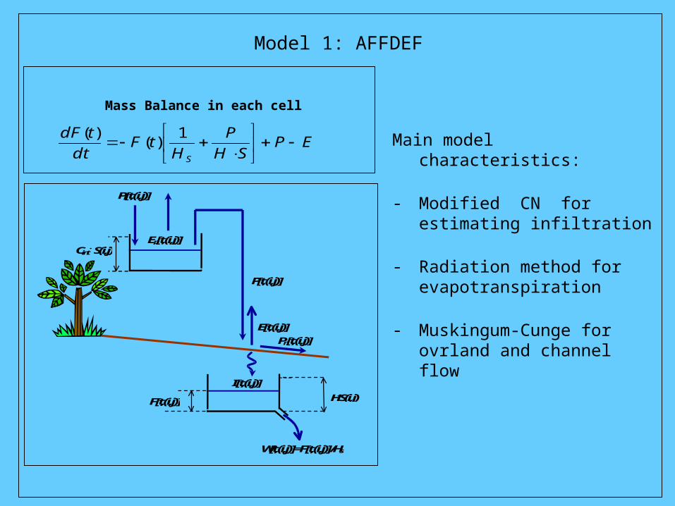
TOPKAPI Distributed approachParameters

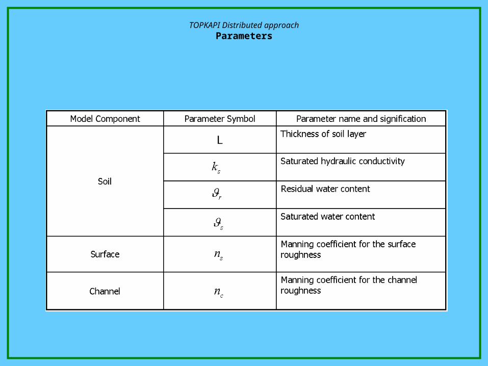
Model 3: MIKE SHE

Main model characteristics:

- 1D Richards equations for unsaturated zone

- 3D Boussinesq equation for greoundwater

- Parabolic approximation for overland flow

)()(

))(( zSz

K

zK

zt

t

hSQ

z

hK

zy

hK

yx

hK

x zzyyxx

)()()(

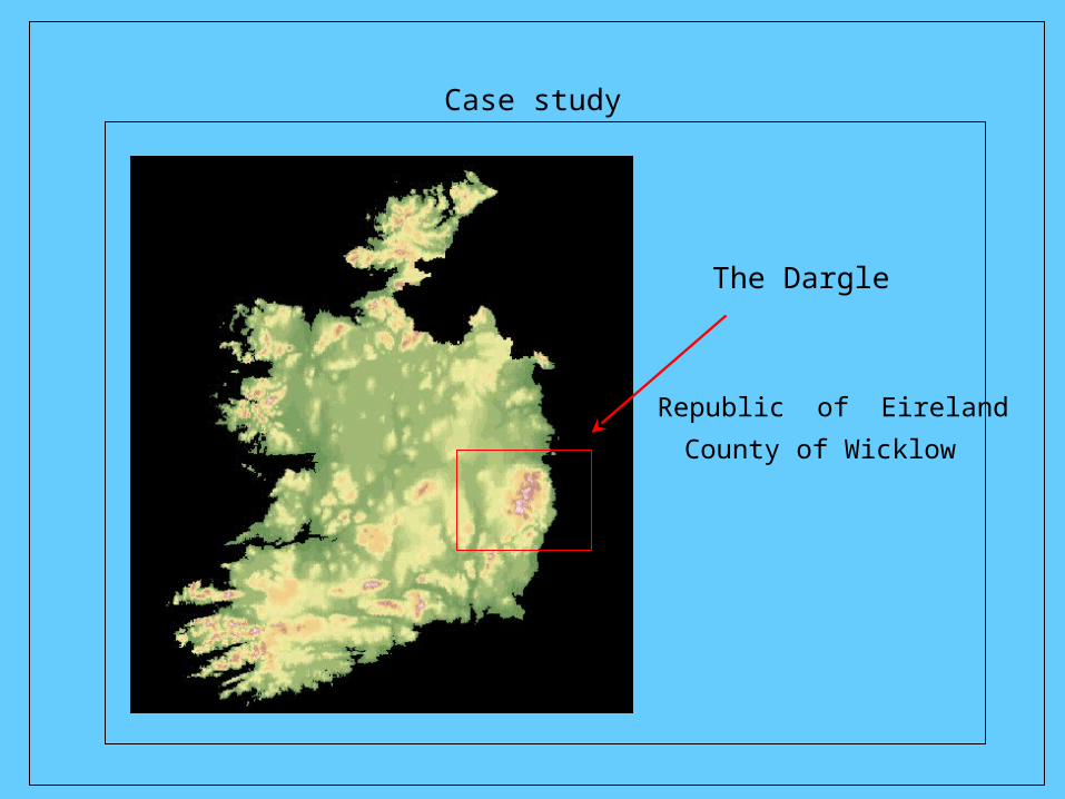
Case study

The Dargle

County of Wicklow

Republic of Eireland

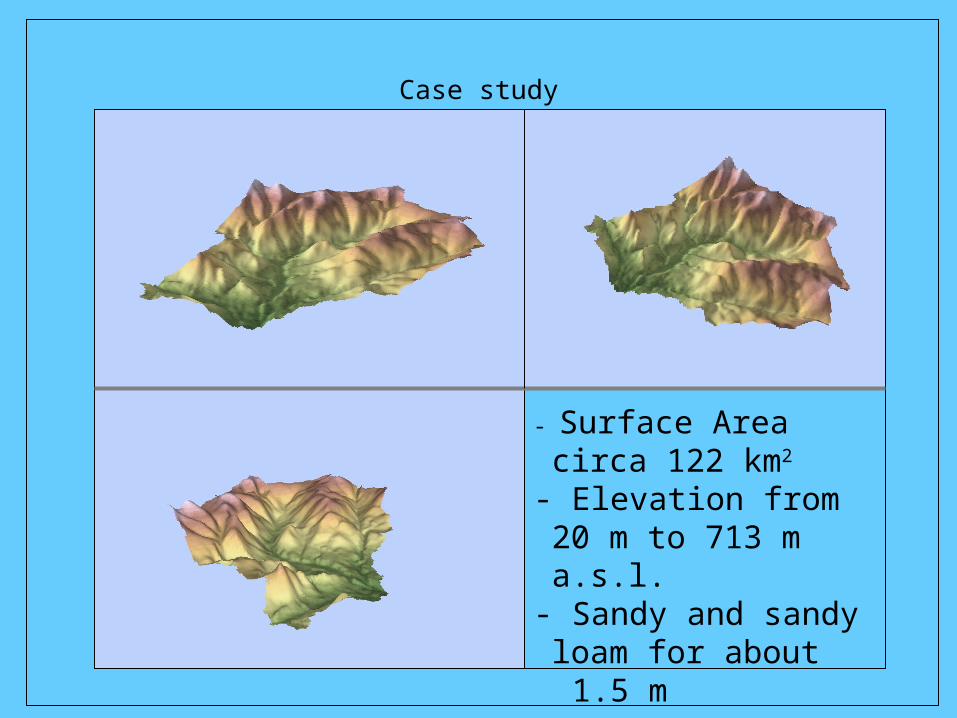
Case study

- Surface Area circa 122 km2

- Elevation from 20 m to 713 m a.s.l.

- Sandy and sandy loam for about

1.5 m

Saturation mechanism

Horton Dunne

The “unrealistic” profile used in MIKE

SHE

to meet the observations

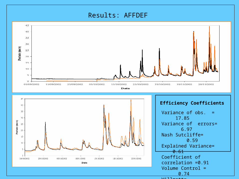
Results: AFFDEF

Variance of obs. = 17.85 Variance of errors= 6.97Nash Sutcliffe= 0.59Explained Variance= 0.61 Coefficient of correlation =0.91 Volume Control = 0.74 Willmott= 0.93

Efficiency Coefficients

Risults: AFFDEF

Uniform value for curve number: 20

0.01 [ms-1]

5 [Km2 ]Areal threshold

Saturated Hydraulic Conductivity

Infiltration Res. Const 4320000[s]

Infiltration constant 0.7

Infiltration Capacity 0.1

Average computer time = 5 min



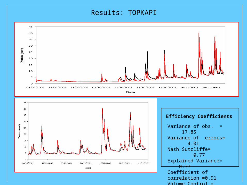
Results: TOPKAPI



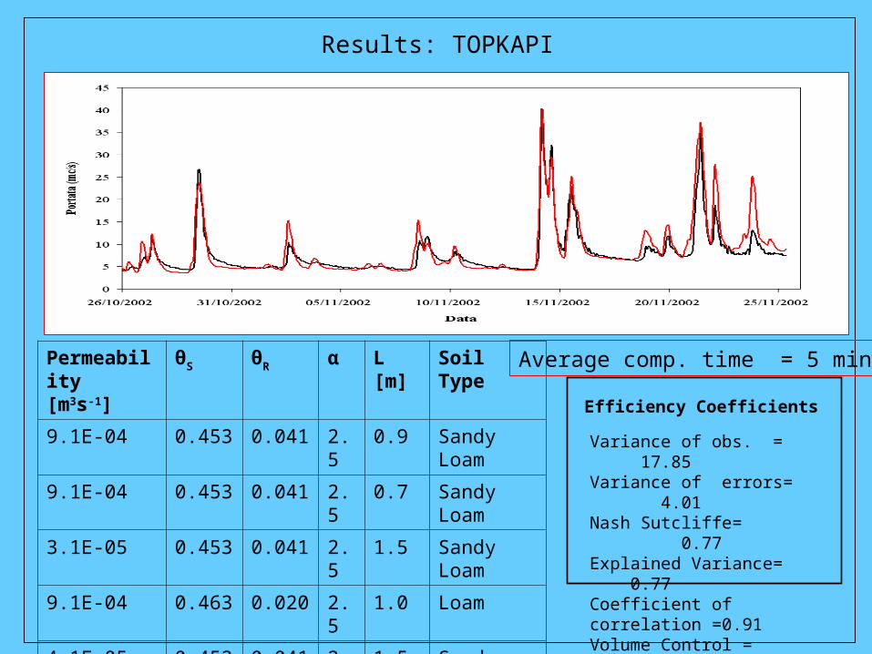
Results: TOPKAPI

Permeability[m3s-1]

θS θR α L[m]

Soil Type

9.1E-04 0.453 0.041 2.5 0.9 Sandy Loam

9.1E-04 0.453 0.041 2.5 0.7 Sandy Loam

3.1E-05 0.453 0.041 2.5 1.5 Sandy Loam

9.1E-04 0.463 0.020 2.5 1.0 Loam

4.1E-05 0.453 0.041 2.5 1.5 Sandy Loam

9.1E-04 0.463 0.020 2.5 0.7 Loam



Average comp. time = 5 min

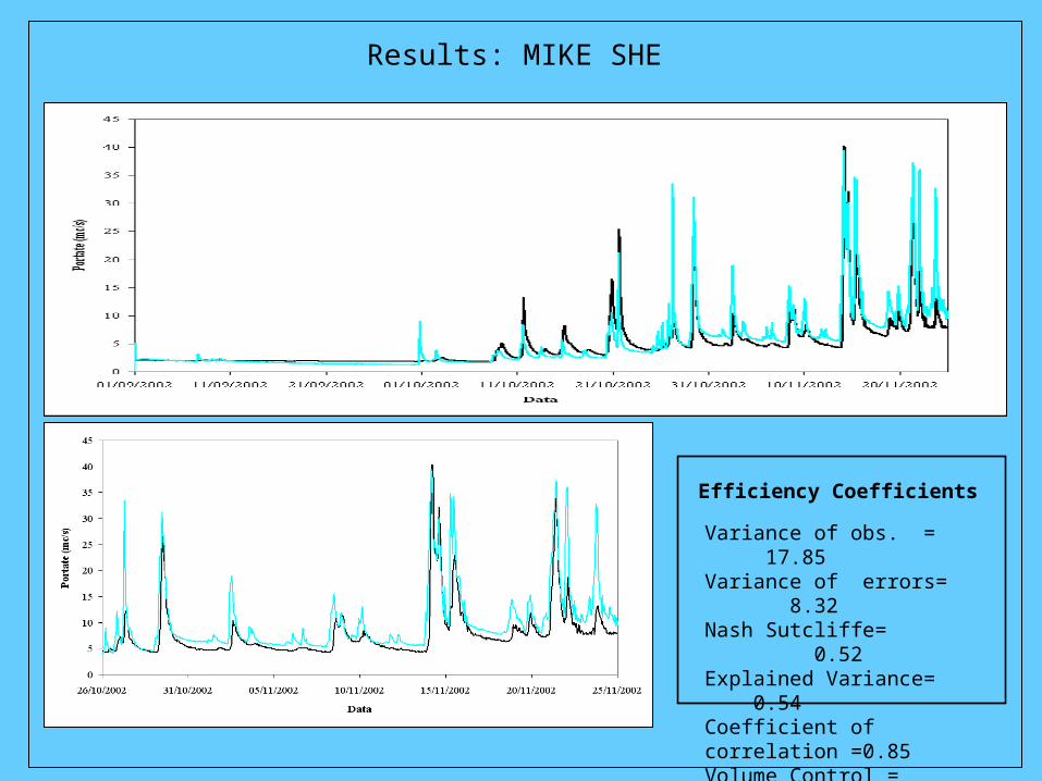
Results: MIKE SHE

Variance of obs. = 17.85 Variance of errors= 8.32Nash Sutcliffe= 0.52Explained Variance= 0.54Coefficient of correlation =0.85 Volume Control = 0.80 Willmott= 0.90


Results: MIKE SHE

Thickness of soil layer -1.3 [m]

Horizontal hydraulic conductivity 5*10-4 [m s-1]

Vertical hydraulic conductivity 1*10-5 [m s-1]

Storativity coefficient 0.2 [m-1]

Variance of obs. = 17.85 Variance of errors= 8.32Nash Sutcliffe= 0.52Explained Variance= 0.54Coefficient of correlation =0.85 Volume Control = 0.80 Willmott= 0.90


Average computer time = 2.5 h

Distributed soil moisture

Saturation percentage

TOPKAPI CALIBRATION TOOL

Example of link ECMWF -TOPKAPI on the Po Basin

The basin closed at Ponte Spessa (Surface area 36,900 km2 )

Ponte Spessa

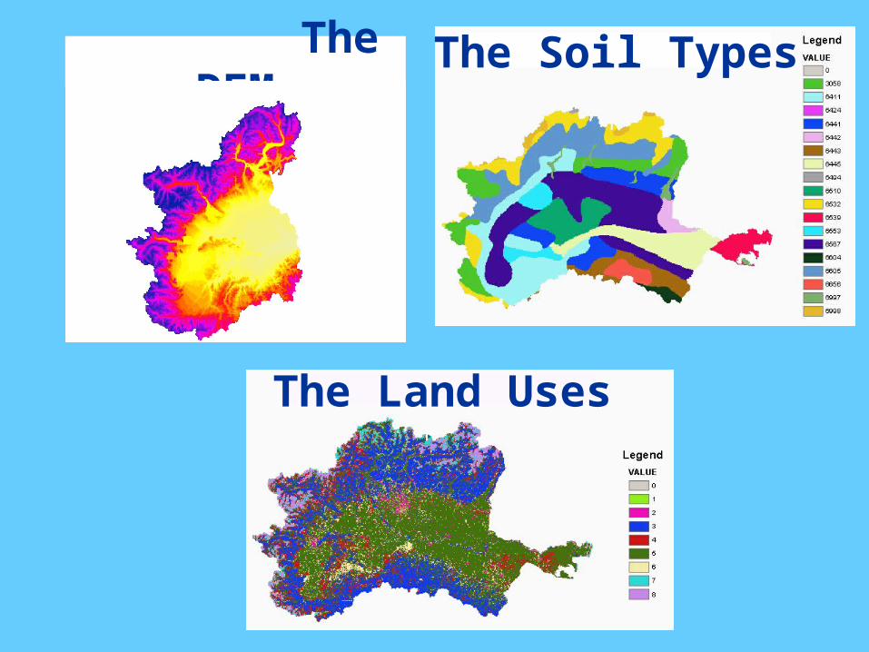
The DEM The Soil Types

The Land Uses

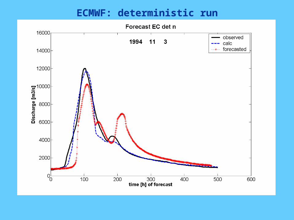
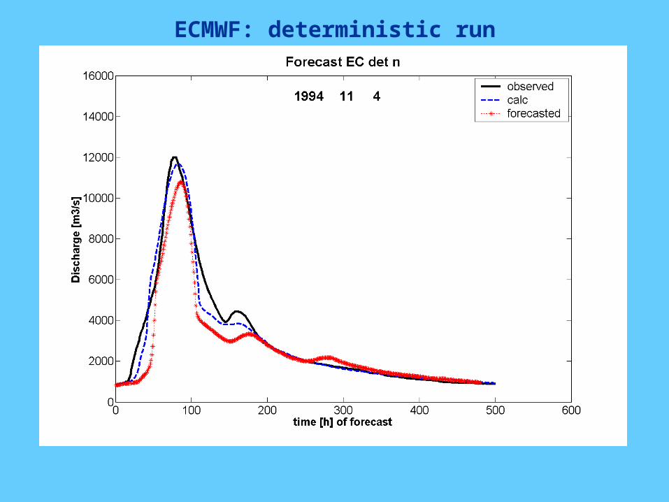
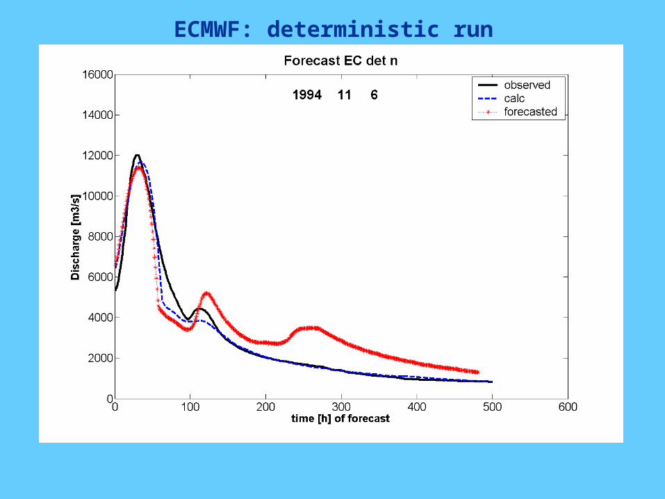
Reproduction of the 1994 event in the Po river

ECMWF: deterministic run





Documents

DISTRIBUTED RAINFALL RUNOFF MODELS APPLIED TO THE DARGLE