Distributed Lasso

CME 323 Project Report

Sebastien DUBOIS, Sebastien LEVY

06/05/2016

1

Contents

Introduction 3

1 Lasso Regression 31.1 Definition, Penalization and Sparsity . . . . . . . . . . . . . . . . . . . . . . . 31.2 Sequential Solving Methods . . . . . . . . . . . . . . . . . . . . . . . . . . . . 4

1.2.1 Gradient Methods . . . . . . . . . . . . . . . . . . . . . . . . . . . . . 41.2.2 Coordinate Descent . . . . . . . . . . . . . . . . . . . . . . . . . . . . 51.2.3 Least Angle Regression . . . . . . . . . . . . . . . . . . . . . . . . . . 5

2 Parallelization 62.1 Objectives . . . . . . . . . . . . . . . . . . . . . . . . . . . . . . . . . . . . . . 62.2 Existing methods . . . . . . . . . . . . . . . . . . . . . . . . . . . . . . . . . . 7

2.2.1 Using SGD (Spark) . . . . . . . . . . . . . . . . . . . . . . . . . . . . 72.2.2 Shotgun (Distributed Coordinate Descent) . . . . . . . . . . . . . . . . 8

2.3 What about Least Angle Regression ? . . . . . . . . . . . . . . . . . . . . . . 8

3 Sequential LARS algorithm 93.1 General idea . . . . . . . . . . . . . . . . . . . . . . . . . . . . . . . . . . . . . 93.2 Algorithm . . . . . . . . . . . . . . . . . . . . . . . . . . . . . . . . . . . . . . 93.3 Proof . . . . . . . . . . . . . . . . . . . . . . . . . . . . . . . . . . . . . . . . . 103.4 Matrix inversion and Cholesky decomposition . . . . . . . . . . . . . . . . . . 103.5 Lasso path from LARS? . . . . . . . . . . . . . . . . . . . . . . . . . . . . . . 11

4 D-LARS for ’Short and Fat’ matrices (n� p) 114.1 Set up . . . . . . . . . . . . . . . . . . . . . . . . . . . . . . . . . . . . . . . . 114.2 Algorithm . . . . . . . . . . . . . . . . . . . . . . . . . . . . . . . . . . . . . . 124.3 Spark Implementation . . . . . . . . . . . . . . . . . . . . . . . . . . . . . . . 144.4 Complexity . . . . . . . . . . . . . . . . . . . . . . . . . . . . . . . . . . . . . 154.5 Discussion . . . . . . . . . . . . . . . . . . . . . . . . . . . . . . . . . . . . . . 16

5 D-LARS for ’Tall and Skinny’ matrices (p� n) 165.1 Set up . . . . . . . . . . . . . . . . . . . . . . . . . . . . . . . . . . . . . . . . 165.2 Algorithm . . . . . . . . . . . . . . . . . . . . . . . . . . . . . . . . . . . . . . 175.3 Complexity . . . . . . . . . . . . . . . . . . . . . . . . . . . . . . . . . . . . . 195.4 Discussion . . . . . . . . . . . . . . . . . . . . . . . . . . . . . . . . . . . . . . 19

6 D-LARS for ’Almost Square’ matrices (n ∼ p) 206.1 Set up . . . . . . . . . . . . . . . . . . . . . . . . . . . . . . . . . . . . . . . . 206.2 Computing the whole path . . . . . . . . . . . . . . . . . . . . . . . . . . . . 21

6.2.1 Distributed Cholesky . . . . . . . . . . . . . . . . . . . . . . . . . . . . 216.2.2 Solving the linear system by gradient descent . . . . . . . . . . . . . . 236.2.3 Incremental Forward Stagewise approximation . . . . . . . . . . . . . 24

Conclusion 24

Appendix: Code sample 26

2

Introduction

The Lasso is a simple linear model used to tackle a wide range of machine learning problems.By adding a L1 penalization to the ordinary least squares, it induces sparsity in the coeffi-cients, making the algorithm very efficient even when the number of features is bigger thanthe number of observations. Another interesting characteristic of the Lasso is its piece-wiselinear coefficient path, which can be leveraged for efficient computations. Although sim-ple gradient methods can be applied to solve the underlying convex minimization problem,there exists a couple of exact methods which are as efficient, if not faster. Such methodsare usually preferred in sequential frameworks to guarantee sparsity and compute the wholecoefficient path.

In this project, we propose a distributed algorithm to solve the Lasso based on LeastAngle Regression (LARS). Our algorithm guarantees the sparsity of the solution, can handleall types of distributed matrices, and computes the whole coefficient path. We show thatthe complexity of the proposed algorithm is promising, since the communication cost iscomparable to gradient methods, while providing a useful parallelization of the sequentialversion (similar amount of total work, logarithmic depth in the large dimension).

This report is organized as follows. First, we briefly present the Lasso and differentmethods to solve it. Then, we discuss various challenges in its parallelization and reviewexisting attempts to solve the Lasso in distributed frameworks. This leads us to focus onLARS, which algorithm is detailed in section 3. We finally propose a distributed versionof LARS (D-LARS) for three types of data matrices: ’Short and Fat’ (section 4), ’Tall andSkinny’ (section 5), and ’Almost Square’ (section 6). In each case, we provide pseudo-codeto reflect the challenges of the implementation, and analyze the complexity in terms of com-munication cost and computation time. We conclude on why we think the proposed methodis promising by comparing it with existing solutions, especially SGD-based implementations.

1 Lasso Regression

1.1 Definition, Penalization and Sparsity

The Lasso regression is a linear regression with a L1 penalization. The penalization termadded to the ordinary least squares creates bias but decreases the variance. Since the meansquare error (the quantity to minimize) is the sum of the squared bias and variance, we canoften achieve better accuracy by optimizing the regularization coefficient to reach optimaltrade-off.

Compared to other types of penalization, the main advantage of the L1 norm is that itcombines two great advantages, sparsity and convexity. While staying convex and guaran-teeing a unique minimum, it induces sparsity in the coefficients, i.e. a lot of the coefficientsare zero. This is a real advantage for interpretability, computing time and storage memory.This type of penalization is also well adapted to cases where p > n. Indeed, there would bean infinite number of solutions without penalization, but the L1 norm insures uniqueness ofthe solution, with at most n predictors in the model (those with non-zero coefficient).

The minimization problem to solve is the following:

argminβ

n∑i=1

(XTi β − yi)2 + λ

p∑j=1

|βj |

3

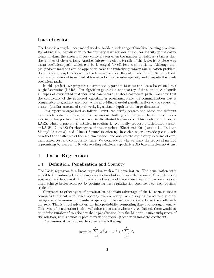
The λ coefficient is the regularization parameter. By changing its value we can find thecoefficient path (the values of each coefficient for every value of λ). It has the particularityto be piece-wise linear for the Lasso, and slopes change only when a new variable enters theset of active variables (those with non-zero coefficient).

Figure 1: Example of a Lasso coefficient path (Figure 3.10 in [5])

Besides providing insight on the model and the different importance of features, it canalso ease the search for optimal λ by cross-validation. With the path, we have all thecoefficients for every value of λ.

The interest of studying Lasso extends to other interesting methods. By adding, inaddition to the L1 penalty, an L2 penalty we get the Elastic Net. This version combinesthe advantages of Lasso but handles correlated features better. The L1 penalty can alsobe added to more complicated methods in a similar way. The most popular are logisticregression, nearest neighbors, LDA and SVM. It is also used in boosting methods.

1.2 Sequential Solving Methods

1.2.1 Gradient Methods

The simplest way to solve the optimization problem is to simply use any general gradientbased solving method. The convexity of the loss function guarantee to find the globalminimum. Two methods are mostly used to solve this problem: gradient descent andstochastic gradient descent (SGD). Because the penalty is not differentiable in 0, equivalentsubgradient methods are used.

At each step, the gradient descent method simply computes the gradient of the quantityto minimize and moves of a step η in the other direction. This will converge quite quickly:

4

to get a precision ε, we will need only O(log(

1ε

))iterations. However, at each step we

will need to see all the observations making the iterations long, and somehow useless in thebeginning where an accurate estimation of the best direction to go is not essential.

Another alternative, is stochastic gradient descent (SGD) in which we use the fact thatthe minimizing function can be written as a sum of differentiable function (except in 0). Wewill then compute the gradient of all the elements of the sum and update them one afterthe other. At each pass (all the observations give their update), we shuffle the data. Thismethods has much smaller iterations but need O

(1ε

)iterations to converge with a precision

ε.The main advantage of those methods are that they can give a good approximation of

the solution quite rapidly. The methods are really simple, only need the gradient (no order2 differentials) and are very general. However, on the particular optimization problem ofLasso, approximating the solution tends to lose the sparsity [7], the solutions won’t havemany zero coefficients but small values instead. Although we could hard threshold thecoefficients, we would still get more computations and more memory needed to store all thenon-zero coefficients. The method is also less adapted to compute the whole coefficient path.It can use solutions from a close value of λ as a warm start but would still need to solvemany optimization problems and won’t take advantage of the piece-wise linear property ofthe path.

1.2.2 Coordinate Descent

Coordinate Descent [3] is the most recent of the successful methods proposed to computethe Lasso path (and actually to solve any Elastic-Net). This algorithm is known to be veryfast, and is the one used in the well-known R package glmnet.

The basic idea behind coordinate descent is to start with an estimate β and update eachof its entries one by one, using the gradient of the objective function (loss + L1 penalty)considering all but one entries fixed.

In practice, the coordinate descent algorithm starts with β = 0 (corresponding to aninfinite penalty λ =∞), and slightly decreases the value of the regularization parameter λafter a solution is found.

This technique has proved to be very efficient because it leverages the fact that most ofthe coefficients are zero as well as warm starts, while computing the whole coefficient path.Therefore, the algorithm must do a lot of iterations (for many different values of λ) but eachof them requires only a few step. This technique also guarantees sparsity in the coefficients.

1.2.3 Least Angle Regression

Least Angle Regression (LARS) is a solving technique based on the computation of thecoefficient path, taking advantage of its piece-wise linear property. It was originally proposedby Efron et al. [2] as a new forward selection method. The coefficient path it computes wasfound out to be very similar to the Lasso path. The path is actually the exact same whenno coefficient crosses zero in the path. By slightly modifying the algorithm (see section 3.5),the exact Lasso solution can be computed in any cases. Before the emergence of coordinatedescent, it was the main technique to solve this problem.

The algorithms starts with all coefficients to zero, it finds the predictor most correlatedwith the residual, and increases its coefficient until another predictor is equally correlatedwith the residual. Then, it increases both coefficients in a way that keeps the correlationstied, until another predictor is equally correlated with the residual, etc . . . This can be

5

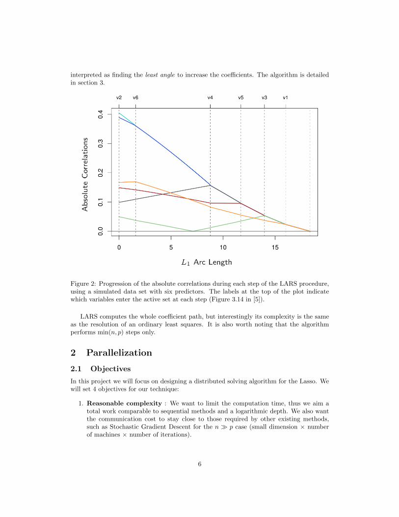
interpreted as finding the least angle to increase the coefficients. The algorithm is detailedin section 3.

Figure 2: Progression of the absolute correlations during each step of the LARS procedure,using a simulated data set with six predictors. The labels at the top of the plot indicatewhich variables enter the active set at each step (Figure 3.14 in [5]).

LARS computes the whole coefficient path, but interestingly its complexity is the sameas the resolution of an ordinary least squares. It is also worth noting that the algorithmperforms min(n, p) steps only.

2 Parallelization

2.1 Objectives

In this project we will focus on designing a distributed solving algorithm for the Lasso. Wewill set 4 objectives for our technique:

1. Reasonable complexity : We want to limit the computation time, thus we aim atotal work comparable to sequential methods and a logarithmic depth. We also wantthe communication cost to stay close to those required by other existing methods,such as Stochastic Gradient Descent for the n � p case (small dimension × numberof machines × number of iterations).

6

2. Guarantee sparsity : The sparsity in the coefficients is one of the major interestsof the Lasso. For very big models (p � n or p ∼ n), we can easily assume that thenumber of relevant predictors should remain small. Regarding the complexity of thealgorithm, sparsity has also two advantages:

• having many zero values largely decrease the storage necessary

• in a distributed framework, we will need to communicate the coefficient esti-mate between different machines, therefore its sparsity will help controlling thecommunication required by the algorithm.

To guarantee sparsity, it would then be interesting to focus on exact solving methods.

3. Whole coefficient path : As explained before, an interesting feature of the Lassomethod is its piece-wise linear coefficient path. Various sequential solving methods canoutput the whole path for a similar computational cost (LARS, Coordinate Descent).This path can be used to grasp a better understanding of the model studied and toget the optimal penalization coefficient (λ) by cross validation without computationoverhead.

4. All types of matrices : An important advantage of the Lasso is its ability to dealwith problems where p ∼ n or p � n. Indeed, the solution is unique thanks to theregularization, and the solution’s sparsity guarantees interpretability. The last case,n� p, is very common in machine learning problem, especially in medicine or biology.Thus, we find it really valuable to design algorithms which can deal with the threetypes of data matrices outlined previously.

We will show in the next parts that the existing methods do not satisfy those 4 objectives.This justify the development of a new distributed method based on Least Angle Regression.

2.2 Existing methods

In the distributed framework, only two methods are really implemented to solve the Lasso:

2.2.1 Using SGD (Spark)

On Spark, like various other regression and classification methods, the Lasso is solved usingstochastic gradient descent. To avoid shuffling the data, which would imply a large commu-nication cost (O(np)), distributed sampling is used on the observations at each iteration. Asubgradient is used to deal with non differentiability of the L1 norm in 0.

This method does not satisfy 2 of our 4 objectives. By computing approximate solutions,we lose the sparsity in the coefficients [7]. Like the sequential version, it does not compute thefull coefficient path, and although warm starts could be used, we would need to solve a largenumber of optimization problems to get it which would involve unreasonable complexities.Moreover, this method is only really adapted to the n � p case. It is implemented formatrices distributed by rows and the big advantage of SGD is that it can stop before seeingall the observations.

Because it fails at most of our objectives, we decide to discard this method for thisproject and to explore distributed version of other solving methods.

7

2.2.2 Shotgun (Distributed Coordinate Descent)

The Shotgun method developed by Bradley et al [1] is a distributed version of the shootingmethod (Coordinate Descent). The general idea is to update the coefficients as in the sequen-tial coordinate descent, but in parallel. The resulting method works well with uncorrelatedfeatures but updates can conflict when correlations are too large.

It has been proved that the number of machines on which it can be parallelized withoutdiverging depends on the biggest eigenvalue of XTX: ρ (at most p

ρ +1). This is problematic

since this quantity would be too costly to compute in general (note that XTX do not fitin memory when p � n). In addition, when ρ is too large, we would only be able tooparallelize the algorithm by making several machines work on the same update. But thiswould yield important communication cost and suboptimal algorithm. Other techniques toavoid divergence would be to lock when performing an important update but that would goagainst our distributed framework.

The need to solve the optimization problem for a large set of values of λ would alsoinvolve unreasonable communication cost. Another disadvantage of this method is that it isonly adapted to matrices stored by columns. When n� p and if it is stored by rows, onceagain, there will be communication issues.

Finally, Zeng et al. compared the performances of the Shotgun algorithm on differentmachine learning platforms [9]. They report poor results on Spark compared to the otherframeworks, which let us think this method is not well suited for Spark (which is ourtargeted framework). In addition, they claim this was due to an excess of communication(even though they study this algorithm on Short and Fat matrices p� n).

It is clear that this algorithms does not satisfy our objectives. Moreover, its convergenceto the solution depends a lot on the data, which is not something desirable.

2.3 What about Least Angle Regression ?

In section 1.2 we presented the three most famous methods to solve the Lasso sequentially.Attempts were made to design a distributed version of the first two, but as described abovewe found they had several drawbacks. Thus, it seems reasonable to look at the third option:Leas Angle Regression. By essence, it guarantees the sparsity and computes the whole path.We also know that the computation of the path does not add any overhead in the sequentialframework.

Another main advantage is that it is based on the covariance matrix of the active vari-ables, whose size cannot exceed the smallest dimension (min(n, p)). It is therefore welladapted to cases where n � p and n � p. The number of iterations of the algorithm isalso quite small in those cases (min(n, p)). Most of the operations appear embarrassinglyparallel (finding the next feature to enter the model, normalizing the data, updating thecoefficients) or easily doable on the driver (solving linear system). We will see that we canalso deal with almost square matrices with either an incomplete path, by approximation, orby increasing the communication cost.

In the next part, we will study the full sequential algorithm and we will then studyseparately the distributed algorithm for each one of the three types of matrices.

8

3 Sequential LARS algorithm

3.1 General idea

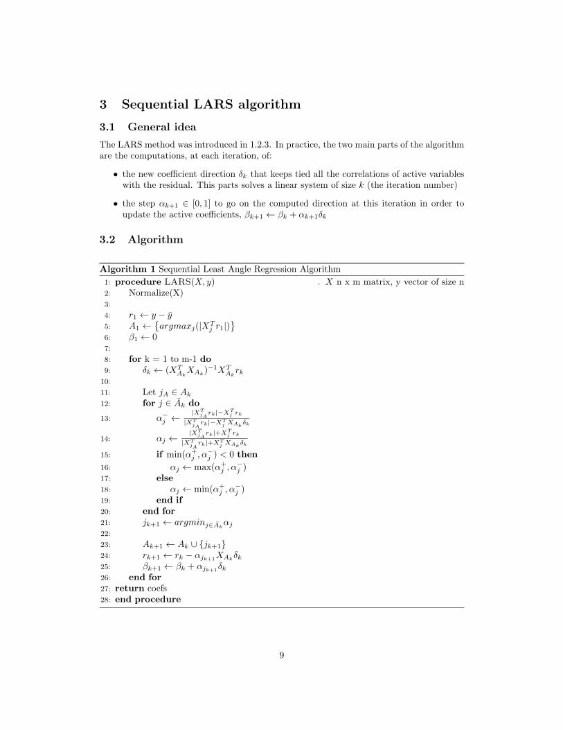
The LARS method was introduced in 1.2.3. In practice, the two main parts of the algorithmare the computations, at each iteration, of:

• the new coefficient direction δk that keeps tied all the correlations of active variableswith the residual. This parts solves a linear system of size k (the iteration number)

• the step αk+1 ∈ [0, 1] to go on the computed direction at this iteration in order toupdate the active coefficients, βk+1 ← βk + αk+1δk

3.2 Algorithm

Algorithm 1 Sequential Least Angle Regression Algorithm

1: procedure LARS(X, y) . X n x m matrix, y vector of size n2: Normalize(X)3:

4: r1 ← y − y5: A1 ←

{argmaxj(|XT

j r1|)}

6: β1 ← 07:

8: for k = 1 to m-1 do9: δk ← (XT

AkXAk

)−1XTAkrk

10:

11: Let jA ∈ Ak12: for j ∈ Ak do

13: α−j ←|XT

jArk|−XT

j rk

|XTjArk|−XT

j XAkδk

14: αj ←|XT

jArk|+XT

j rk

|XTjArk|+XT

j XAkδk

15: if min(α+j , α

−j ) < 0 then

16: αj ← max(α+j , α

−j )

17: else18: αj ← min(α+

j , α−j )

19: end if20: end for21: jk+1 ← argminj∈Ak

αj22:

23: Ak+1 ← Ak ∪ {jk+1}24: rk+1 ← rk − αjk+1

XAkδk

25: βk+1 ← βk + αjk+1δk

26: end for27: return coefs28: end procedure

9

3.3 Proof

We prove in this section why the algorithm above does compute the LARS solution.Using

rk(α) = rk − αXAkδk

we get:XAk

rk(α) = XTAkrk − αXT

AkXAk

δk = (1− α)XTAkrk

which shows that δk is indeed the direction for which all the active variables keep identicalcorrelation with the residual.Also ∀jA ∈ Ak, the correlation is:

Corr(jA, rk(α)) = (1− α)XTjArk

and for any other predictor j :

Corr(j, rk(α)) = XTj rk − αXT

j XAkδk

For each predictor j ∈ Ak, we are looking for the value of αj such that:

|Corr(j, rk(α))| = |Corr(jA, rk(α))|

If Corr(j, rk(α)) > 0, which is equivalent to XTj rk > αXT

j XAkδk, then

α−j =|XT

jArk| −XT

j rk

|XTjArk| −XT

j XAkδk

Otherwise:

α+j =

|XTjArk|+XT

j rk

|XTjArk|+XT

j XAkδk

We can then simplify this expression by taking

αj =

{min(α+

j , α−j ) if min(α+

j , α−j ) ≥ 0

max(α+j , α

−j ) if min(α+

j , α−j ) < 0

3.4 Matrix inversion and Cholesky decomposition

As outlined in the algorithm above, at each step we need to compute the new coefficientdirection δk ← (XT

AkXAk

)−1XTAkrk. This means that we need to solve the linear system

Ckx = XTAkrk where Ck is the covariance matrix between active variables (of size k × k).

A classic method to solve such an equation is to compute the LU decomposition of Ck(in time O(k3)), to then solve two triangular systems (in time O(k2)).

For the LARS algorithm, we can actually do a lot better. First notice that Ck is sym-metric so we actually compute the Cholesky factor Gk such that Ck = GkG

Tk . Also, at each

step Ck is extended by one last column/row, so the first k × k block of Gk+1 is actuallyGk. Hence we only need to compute the last new row of Gk+1 at step k + 1, which is donein k2 only (compared to k3 to compute the whole factor). A few more details on the exactcomputation of the Cholesky factor are given in section 6.2.1.

Therefore, from the first to the last iteration, we store the current Cholesky decomposi-tion of the covariance matrix XT

AkXAk

. It is updated at each step in O(k2) time, and usedto solve the linear system, also in in O(k2) time, giving δk.

This remark decreases the total computations needed for δ1, . . . , δI by a factor I: fromO(I4) to O(I3) (I being the total number of iterations, so typically I = min(n, p)).

10

3.5 Lasso path from LARS?

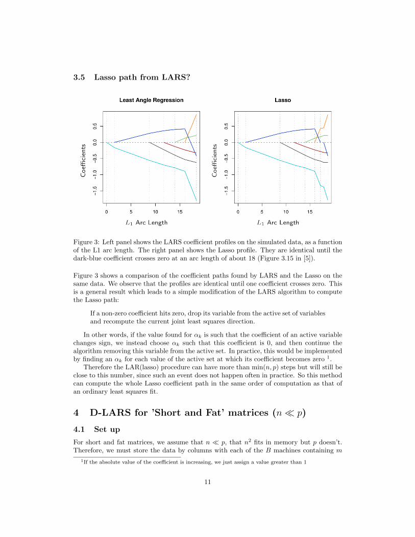
Figure 3: Left panel shows the LARS coefficient profiles on the simulated data, as a functionof the L1 arc length. The right panel shows the Lasso profile. They are identical until thedark-blue coefficient crosses zero at an arc length of about 18 (Figure 3.15 in [5]).

Figure 3 shows a comparison of the coefficient paths found by LARS and the Lasso on thesame data. We observe that the profiles are identical until one coefficient crosses zero. Thisis a general result which leads to a simple modification of the LARS algorithm to computethe Lasso path:

If a non-zero coefficient hits zero, drop its variable from the active set of variablesand recompute the current joint least squares direction.

In other words, if the value found for αk is such that the coefficient of an active variablechanges sign, we instead choose αk such that this coefficient is 0, and then continue thealgorithm removing this variable from the active set. In practice, this would be implementedby finding an αk for each value of the active set at which its coefficient becomes zero 1.

Therefore the LAR(lasso) procedure can have more than min(n, p) steps but will still beclose to this number, since such an event does not happen often in practice. So this methodcan compute the whole Lasso coefficient path in the same order of computation as that ofan ordinary least squares fit.

4 D-LARS for ’Short and Fat’ matrices (n� p)

4.1 Set up

For short and fat matrices, we assume that n � p, that n2 fits in memory but p doesn’t.Therefore, we must store the data by columns with each of the B machines containing m

1If the absolute value of the coefficient is increasing, we just assign a value greater than 1

11

columns – We assume mn fits in memory (m×B = p). We want our algorithm to

• Scale on p, the large dimension

• Avoid All-to-All communications

• Not broadcast more than a constant number of vector of size n at each iteration toevery machine

Because n2 fits in memory and I ≤ n, we will store the covariance matrix on the driver.To be able to easily solve the linear system giving the direction δk ← (XT

AkXAk

)−1XTAkrk,

we store the Cholesky decomposition of the covariance matrix on the driver, and updateit at each iteration. We will also store the current correlation with the residual and thecoefficients of previous iterations on the driver. Each machine will only store its m columns.

4.2 Algorithm

When the data is distributed by columns, we use the following algorithm:

Algorithm 2 Short and Fat - Distributed Least Angle Regression

1: procedure D-LARS(X, y) . X n x p matrix, y vector of size n2:

3: Normalize(X) in parallel . Map4:

5: r1 ← y − y6: Broadcast r1 to every machine7: for j in 1 to p do8: sj ← 2 ∗ 1XT

j r1>0 − 1

9: Emit (j, |XTj r1|, sj) . Map

10: end for11: j1, cor1, s1 ← max(j, |XT

j r1|, sj) . Reduce12:

13: Init(j1, Xj1)14:

15: for k = 1 to n-1 do16:

17: Broadcast rk to every machine18: δk ← ComputeDelta(cork, XAk

, s)19: jk+1, αk+1, sjk+1

← minj∈AkEmitAlpha(δk, cork, Ak) . Reduce

20:

21: Ak+1 ← Ak ∪ {jk+1}22: cork+1 ← (1− αk+1)cork23: UpdateEstimates(jk+1, αk+1, XAk

, Xk+1)24:

25: end for26: return β27: end procedure

The pseudo-code for Init, ComputeDelta, EmitAlpha and UpdateEstimates isprovided below. Note that since n � p, the Cholesky factor as well as the n × n matrix

12

containing the coefficients of the path are stored on the driver. The computations of δk andAkδk are also done on the driver.

Algorithm 3 Short and Fat Init

1: procedure Init(j1, Xj1)2: A1 ← {j1}3: G1 ←

(XTj1Xj1

)4: β ← SparseMatrix of zeros (n× n)5: end procedure

Algorithm 4 Short and Fat ComputeDelta

1: procedure ComputeDelta(cork, XAk, sAk

)2: . Locally3: Compute the new column of the covariance matrix XT

AkXAk

from dot product of newactive variable with previously selected ones

4: Extend the Cholesky factor Gk with new row, so that GkGTk = XT

AkXAk

5:

6: ck ← cork ∗ sAk. XT

Akrk

7: δk ← solve(GkGTk x = ck) . Locally

8: return δk9: end procedure

Algorithm 5 Short and Fat EmitAlpha

1: procedure EmitAlpha(δk, cork, Ak, XAk)

2: Compute and Broadcast Xk ← XAkδk . Map + n Reduce

3:

4: for j ∈ Ak do

5: α−j ←(cork −XT

j rk) (cork −XT

j Xk

)−1

6: α+j ←

(cork +XT

j rk) (cork +XT

j Xk

)−1

7: if min(α+j , α

−j ) < 0 then

8: αj ← max(α+j , α

−j )

9: else10: αj ← min(α+

j , α−j )

11: end if12: if αj = α+

j then13: sj ← +114: else15: sj ← −116: end if17: Emit (j, αj , sj) . Map18: end for19: end procedure

13

Algorithm 6 Short and Fat UpdateEstimates

1: procedure UpdateEstimates(jk+1, αk+1, XAk, Xjk+1

)2: // Update Cholesky factor3: Broadcast Xjk+1

to Ak4: for j ∈ Ak do5: Emit (j,XT

j Xjk+1) . Map

6: end for

7: Cov:,k+1 ←(

XTAkXjk+1

1

)new column of the covariance matrix

8: Gk+1 ← Update Cholesky factor Gk . Locally9:

10: // Update residual11: rk+1 ← rk − αk+1 Xk . Locally12:

13: // Update coefficients14: for j ∈ Ak do15: βk+1,j ← βk,j + αk+1 δk,j . Locally16: end for17: end procedure

4.3 Spark Implementation

We implemented the algorithm outlined above in Scala / Spark on Databricks. A note-book with full code and examples can be found at http://bit.do/dlars_databricks. Inaddition, an extract of the core of the code is given in Appendix.

For simplicity, and due to the short time frame of this project, we did not use theCholesky factor but rather stored the covariance matrix. The linear system is solved ateach step with breeze.linalg. However we still implemented the smart update of thecovariance matrix, so this does not impact the communication, but only the computationtime on the driver.

We tested our code on two data sets:

• The lpsa.data set provided in Spark MLlib 2

• A crime data set 3 from the UCI Machine Learning Repositery [6].

In both cases we compared our results with the LARS implementation in R, and foundidentical coefficient paths.

These data sets both have a rather small number of features and observations, and areonly intended to highlight the correctness of the implementation. Indeed, our Databricksaccount was not well fitted to handle very large amount of data. This is also why we do notreport execution times or experimentally compare it with other implementations such hasLassoWithSGD implemented in Spark.

2data can be found at https://github.com/apache/spark/blob/master/data/mllib/ridge-data/lpsa.

data3information can be found at http://archive.ics.uci.edu/ml/datasets/Communities+and+Crime+

Unnormalized

14

4.4 Complexity

Let’s suppose we only have B machines, each one containing m columns (m×B = p). Thecomplexity analysis is then:

• Normalizing in parallel and computing y − y takes T = O(mn).

• Broadcasting r1 to every machine takes communication C = O(nB) and T = O(n log(B)).

• Finding the maximum correlation takes T = O(log(B) + mn) time and C = O(B)communication. We first compute the correlation in each machine (O(mn)), combinewithin each machine by taking the max (O(m)) and send those values (T = O(log(B))and C = O(B))

• The Init takes T = O(1) time.

• For the kth loop:

– the broadcast takes C = O(nB) communication and T = O(n log(B)) time

– ComputeDelta is done locally and takes time T = O(k2) since the linear systemis solved using the Cholesky decomposition of the covariance matrix (as detailedin section 3.4).

– EmitAlpha takes T = O(kn) to compute Xk, T = O(n log(B)) to broadcastit, T = O(mn) to compute XT

j rk and XTj Xk, T = O(m) to take the minimum

within each machine, and T = O(log(B)) to emit each αj . This gives a totaltime of T = O(kn + n log(B) + mn). The communication is C = O(nB) due tothe first broadcast.

– Taking the minimum of the αj sent by each machine, by doing a reduce, takesT = O(log(B)) and C = O(B).

– Updating Ak, rk and cork takes T = O(1) because XAkδk is already computed.

– UpdateCholesky takes communication C = O(min(k,B)) and time T = O(min(k,B)+k2 + min(k,m)n) = O(k2 + min(k,m)n) to compute the correlations on each ma-chine (min(k,m)n), send them to the driver (min(k,B)) and update the Choleskydecomposition (see section 3.4).

This gives asymptotically (O are omitted):

T = mn+ n log(B) +

I∑k=1

(n log(B) + k2 + nk +mn

)= mnI + n log(B)I + I3 + nI2

{T = O(mnI + n log(B)I + I3 + nI2)

C = O(nB +

∑Ik=1 nB

)= O(nBI)

15

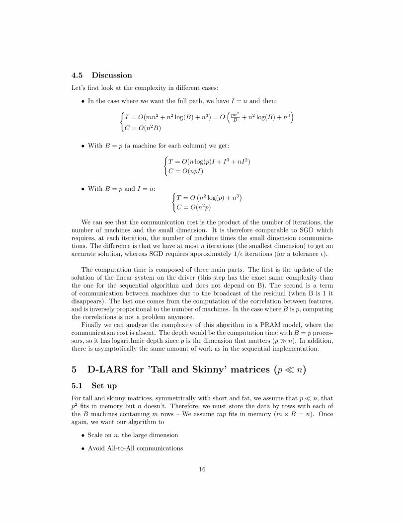
4.5 Discussion

Let’s first look at the complexity in different cases:

• In the case where we want the full path, we have I = n and then:{T = O(mn2 + n2 log(B) + n3) = O

(pn2

B + n2 log(B) + n3)

C = O(n2B)

• With B = p (a machine for each column) we get:{T = O(n log(p)I + I3 + nI2)

C = O(npI)

• With B = p and I = n: {T = O

(n2 log(p) + n3

)C = O(n2p)

We can see that the communication cost is the product of the number of iterations, thenumber of machines and the small dimension. It is therefore comparable to SGD whichrequires, at each iteration, the number of machine times the small dimension communica-tions. The difference is that we have at most n iterations (the smallest dimension) to get anaccurate solution, whereas SGD requires approximately 1/ε iterations (for a tolerance ε).

The computation time is composed of three main parts. The first is the update of thesolution of the linear system on the driver (this step has the exact same complexity thanthe one for the sequential algorithm and does not depend on B). The second is a termof communication between machines due to the broadcast of the residual (when B is 1 itdisappears). The last one comes from the computation of the correlation between features,and is inversely proportional to the number of machines. In the case where B is p, computingthe correlations is not a problem anymore.

Finally we can analyze the complexity of this algorithm in a PRAM model, where thecommunication cost is absent. The depth would be the computation time with B = p proces-sors, so it has logarithmic depth since p is the dimension that matters (p� n). In addition,there is asymptotically the same amount of work as in the sequential implementation.

5 D-LARS for ’Tall and Skinny’ matrices (p� n)

5.1 Set up

For tall and skinny matrices, symmetrically with short and fat, we assume that p� n, thatp2 fits in memory but n doesn’t. Therefore, we must store the data by rows with each ofthe B machines containing m rows – We assume mp fits in memory (m × B = n). Onceagain, we want our algorithm to

• Scale on n, the large dimension

• Avoid All-to-All communications

16

• Not broadcast more than a constant number of vector of size n at each iteration toevery machine

Because p2 fits in memory and I ≤ p, we will also store the covariance matrix on the driver.To be able to easily solve the linear system giving the direction δk ← (XT

AkXAk

)−1XTAkrk,

we store the Cholesky decomposition of the covariance matrix on the driver and updateit at each iteration. We will also store the current correlation with the residual and thecoefficients of previous iterations on the driver. Each machine will only store its m rows.

The main difference is that in this new framework, computing one correlation already re-quires communication between machines. Therefore, we will prefer doing all the correlationsat the same time to take more advantage of the distributed framework.

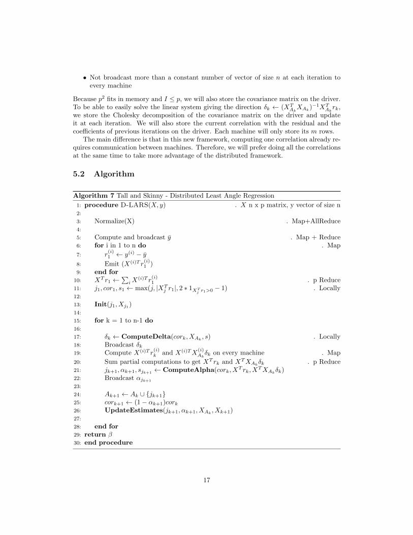
5.2 Algorithm

Algorithm 7 Tall and Skinny - Distributed Least Angle Regression

1: procedure D-LARS(X, y) . X n x p matrix, y vector of size n2:

3: Normalize(X) . Map+AllReduce4:

5: Compute and broadcast y . Map + Reduce6: for i in 1 to n do . Map

7: r(i)1 ← y(i) − y

8: Emit (X(i)T r(i)1 )

9: end for10: XT r1 ←

∑iX

(i)T r(i)1 . p Reduce

11: j1, cor1, s1 ← max(j, |XTj r1|, 2 ∗ 1XT

j r1>0 − 1) . Locally12:

13: Init(j1, Xj1)14:

15: for k = 1 to n-1 do16:

17: δk ← ComputeDelta(cork, XAk, s) . Locally

18: Broadcast δk19: Compute X(i)T r

(i)k and X(i)TX

(i)Akδk on every machine . Map

20: Sum partial computations to get XT rk and XTXAkδk . p Reduce

21: jk+1, αk+1, sjk+1← ComputeAlpha(cork, X

T rk, XTXAk

δk)22: Broadcast αjk+1

23:

24: Ak+1 ← Ak ∪ {jk+1}25: cork+1 ← (1− αk+1)cork26: UpdateEstimates(jk+1, αk+1, XAk

, Xk+1)27:

28: end for29: return β30: end procedure

17

Init and ComputeDelta are implemented as for Short and Fat matrices. ComputeAlphais done locally on the driver with the algorithm below. UpdateEstimates is also slightlydifferent and described below.

Algorithm 8 Tall and Skinny ComputeAlpha

1: procedure ComputeAlpha(cork, XT rk, X

TXAkδk)

2: Let X ← (XTXAk)δk

3: for j ∈ Ak do

4: α−j ←(cork − (XT rk)j

) (cork − Xj

)−1

5: α+j ←

(cork + (XT rk)j

) (cork + Xj

)−1

6: if min(α+j , α

−j ) < 0 then

7: αj ← max(α+j , α

−j )

8: else9: αj ← min(α+

j , α−j )

10: end if11: if αj = α+

j then12: sj ← +113: else14: sj ← −115: end if16: end for

return minj(j, αj , sj)17: end procedure

Algorithm 9 Tall and Skinny UpdateEstimates

1: procedure UpdateEstimates(jk+1, αk+1, XAk, Xjk+1

)2: // Update Cholesky factor3: for i ∈ [1, n] do

4: Emit (X(i)TAk

X(i)jk+1

) . Map5: end for6: Sum to compute the new column of the covariance matrix:7: Cov1:k,k+1 ← XT

AkXjk+1

. k Reduce8: Gk+1 ← Update Cholesky factor Gk . Locally9:

10: // Update residual

11: r(i)k+1 ← r

(i)k − αk+1X

(i)Akδk . Map

12:

13: // Update coefficients14: for j ∈ Ak do15: βk+1,j ← βk,j + αk+1 δk,j . Locally16: end for17: end procedure

18

5.3 Complexity

Assuming we have B machine, each having m rows (mB = n).

• To normalize the data we have to compute the sum of squares for each column, sumit across the machines and finally broadcast the normalization factors. So this takesT = O(pm+ p log(B)) time and C = O(pB) communications. We can also compute ywith the same method and so it does not change the asymptotic complexity.

• Broadcasting y takes time T = O(log(B)) and communication C = O(B).

• Like inside the loop, computing all the correlations using p reduces takes T = O(mp+p log(B))and C = O(pB).

• Init takes T = O(1)

• For the kth loop:

– ComputeDelta is done locally and takes time T = O(k2) since the linear systemis solved using the Cholesky decomposition of the covariance matrix (as detailedin section 3.4).

– Broadcasting δk takes communication C = O(kB) and time T = O(k log(B)).

– We compute XT rk at each step through p dot products between vectors of sizem, before summing across the machines. So this takes T = O (p(m+ log(B))time and C = O(pB) communications.

– The local computation of XTXAkδk takes pm + mk time, and the result is a

vector of size p as above. So we can compute XTXAkδk in T = O(pm+p log(B))

time (since k ≤ p) and C = O(pB) communications.

– We compute αk+1 locally in O(p) time. It is then broadcast, which takes com-munication C = O(B) and time T = O(log(B)).

– UpdateCholesky needs to compute the k dot products XTAkXjk+1

which takestime T = O (k(m+ log(B))) and C = O(kB) communications. The update ofthe Cholesky decomposition takes T = O(k2).

For I iterations, he total complexity is therefore (O omitted){T = Ip (m+ log(B)) + I3

C = IpB

5.4 Discussion

Let’s first look at the complexity in different cases:

• In the case where we want the full path, we have I = p and then:{T = O

(np2

B + p2 log(B) + p3)

C = O(p2B)

19

• With B = n (a machine for each row) we get:{T = O(p log(n)I + I3)

C = O(npI)

• With B = p and I = n: {T = O

(p2 log(n) + p3

)C = O(p2n)

We can see that we have the same kind of complexities we got for Short and Fat matri-ces. All comments regarding Short and Fat then apply (Comparable communication costto SGD, trade off between communication and decreasing the computation time of the cor-relations by changing B).

Even though we could have thought that distributed LARS would be more suitable todata matrices stored by column (n � p), we actually get similar complexities when it isstored by row (p� n). So those symmetric results suggest that the whole method can alsoscale very well on n. This is even more surprising given that computations within machinesare done very differently.

This very strong result is largely due to the LARS method, that only rely on computingthe covariance matrix (correlations). The latter cannot exceed the smallest dimension whichguarantees both a small number of iterations and small matrices, as long as one dimensionis much smaller than the other.

6 D-LARS for ’Almost Square’ matrices (n ∼ p)

6.1 Set up

For almost square matrices, we assume that both n and p fit in memory but that theirsquare n2 and p2 do not. Therefore the data can be stored either by column or row, witheach of the B machines containing m columns/rows – We assume mn fits in memory.

In this scenario the difficulty is that after√n iterations, the covariance matrix of the

active variables do not fit in memory anymore. Therefore we cannot store the Choleskyfactor on the driver if we want more than

√n non-zero coefficients.

Thus we split the analysis of the ’almost square’ case into two parts, depending on thenumber of iterations targeted.

First√n iterations The sparsity of the Lasso solution is its main strength, and can

also be an objective by itself. Therefore when p is large, it can be a reasonable approachto consider only the first

√n steps of the coefficient path (i.e. all solutions with at most√

n non-zero coefficients). The last iterations will in most cases be useless as we won’t getinterpretations and the optimal λ is generally implying few nonzero coefficients when p islarge.

In that case, the covariance matrix / Cholesky factor fit in memory, hence we can store iton the driver. So we can actually use the algorithms proposed for Short and Fat or Tall andSkinny matrices, which interestingly gives flexibility in the way data is stored (by columnor row).

20

6.2 Computing the whole path

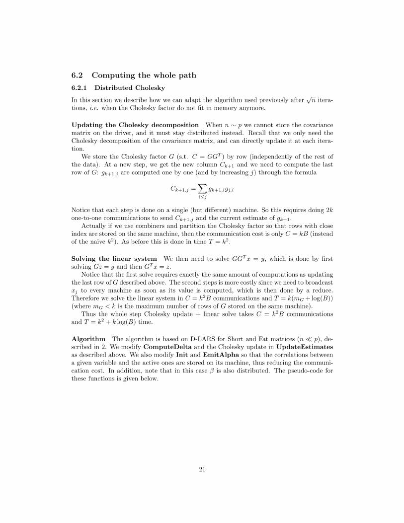
6.2.1 Distributed Cholesky

In this section we describe how we can adapt the algorithm used previously after√n itera-

tions, i.e. when the Cholesky factor do not fit in memory anymore.

Updating the Cholesky decomposition When n ∼ p we cannot store the covariancematrix on the driver, and it must stay distributed instead. Recall that we only need theCholesky decomposition of the covariance matrix, and can directly update it at each itera-tion.

We store the Cholesky factor G (s.t. C = GGT ) by row (independently of the rest ofthe data). At a new step, we get the new column Ck+1 and we need to compute the lastrow of G: gk+1,j are computed one by one (and by increasing j) through the formula

Ck+1,j =∑i≤j

gk+1,igj,i

Notice that each step is done on a single (but different) machine. So this requires doing 2kone-to-one communications to send Ck+1,j and the current estimate of gk+1.

Actually if we use combiners and partition the Cholesky factor so that rows with closeindex are stored on the same machine, then the communication cost is only C = kB (insteadof the naive k2). As before this is done in time T = k2.

Solving the linear system We then need to solve GGTx = y, which is done by firstsolving Gz = y and then GTx = z.

Notice that the first solve requires exactly the same amount of computations as updatingthe last row of G described above. The second steps is more costly since we need to broadcastxj to every machine as soon as its value is computed, which is then done by a reduce.Therefore we solve the linear system in C = k2B communications and T = k(mG + log(B))(where mG < k is the maximum number of rows of G stored on the same machine).

Thus the whole step Cholesky update + linear solve takes C = k2B communicationsand T = k2 + k log(B) time.

Algorithm The algorithm is based on D-LARS for Short and Fat matrices (n � p), de-scribed in 2. We modify ComputeDelta and the Cholesky update in UpdateEstimatesas described above. We also modify Init and EmitAlpha so that the correlations betweena given variable and the active ones are stored on its machine, thus reducing the communi-cation cost. In addition, note that in this case β is also distributed. The pseudo-code forthese functions is given below.

21

Algorithm 10 Square Init

1: procedure Init(j1, Xj1)2: A1 ← {j1}3:

4: Broadcast Xj1

5: for j in 1 to p do6: ActiveCorj ← [XT

j Xj1 ] . Map

7: β(j) ← sparse vector of zeros8: end for9:

10: end procedure

Algorithm 11 Square EmitAlpha

1: procedure EmitAlpha(δk, cork, Ak, XAk)

2: Broadcast δk to every machine3:

4: for j ∈ Ak do5: α−j ←

(cork −XT

j rk)

(cork − ActiveCorjδk)−1

6: α+j ←

(cork +XT

j rk)

(cork + ActiveCorjδk)−1

7: if min(α+j , α

−j ) < 0 then

8: αj ← max(α+j , α

−j )

9: else10: αj ← min(α+

j , α−j )

11: end if12: if αj = α+

j then13: sj ← +114: else15: sj ← −116: end if17: Emit (j, αj , sj) . Map18: end for19: end procedure

22

Algorithm 12 Square UpdateEstimates

1: procedure UpdateEstimates(jk+1, αk+1, XAk, Xjk+1

)2: Broadcast αk+1

3:

4: // Update the distributed Cholesky factor5: Gk+1 ← Update Cholesky factor Gk . Locally6:

7: // Update residual8: rk+1 ← rk − αk+1XAk

δk . Map+Reduce9:

10: // Update coefficients11: for j ∈ Ak do

12: β(j)k+1 ← β

(j)k + αk+1 δk,j . Map

13: end for14: end procedure

6.2.2 Solving the linear system by gradient descent

After√n iterations, we cannot store the covariance matrix on the driver and solving the

linear system, even with the use of distributed Cholesky decomposition, ends up with a lotof communications.

To decrease the communication cost as well as the computation time, we propose the useof approximate solutions for the system. This would be done after the first

√n iterations,

and we suppose that after this point, using approximate coefficient directions would notmuch the path. We can see our linear system as a quadratic optimization problem [8], bynoticing that solving the following system in δ:

XTXδ = XT r

is the same as finding the minimum of f :

f(δ) =1

2δTXTXδ − δTXT r + c

because its gradient is:∇f(δ) = XTXδ −XT r

We can then use any optimization technique to solve this problem, which would provideour next estimate of δk. By using Gradient Descent or SGD with the last estimate as awarm start, we can get a good approximation of the solution without large communicationcosts, and still guaranteeing sparsity in the coefficients (β).

By storing the jth row of XTX on the same machine as the jth column xj , we caneasily perform the updates. We need to broadcast the residual and δ to every machinecontaining active variables, and send the computed δ back. The other steps involve cheapcomputation time and communication cost. With standard gradient descent, each steprequires more computations but takes more advantage of the parallelization to compute theupdate. Whereas SGD does not use parallelization but could converge with less than ksteps.

23

6.2.3 Incremental Forward Stagewise approximation

Incremental Forward Stagewise Regression (FSε) [5] is another path-based linear regressionalgorithm that provides results very similar to Lasso and LARS. Although it was inspiredby boosting procedures, the general idea is very similar to LARS, but with a progressionby small stages along the path. More precisely, it repeats the following steps, with ε > 0 asmall constant:

• Find the predictor Xj most correlated with the residual rk

• Update its coefficient βj ← βj + ε sjk, where sjk is the sign of the correlation betweenXj and the residual

• Update the residual rk+1 ← rk − ε sjkXj

Therefore this method is very similar to LARS but does not need to compute the coeffi-cient directions (i.e. to solve a linear system). Hence we propose to pursue our algorithm,after the first

√n iterations, with this discretized version.

A naive implementation would broadcast Xj or the new residual rk+1 at each step, butthis could drastically increase the communication cost since we cannot bound the numberof iterations. However, we could use some heuristics to avoid that, or increase the stage sizeε. This would result in reducing the number of iterations (speed up), but we would onlyget a discrete path. In addition, we could try other approximations inspired by stochasticgradient descent. For example if the data was stored by row, we could perform many stepson each machine, before merging the results.

Conclusion

We have shown that using specific methods to distribute a targeted problem can lead tobetter parallelization of the algorithm. For the Lasso, using the piece-wise linear property ofits coefficient path, we have been able to outperform generic gradient based solving methods,while satisfying useful objectives. Adapting Least Angle regression has resulted in variousadvantages: it guarantees sparsity and computes the full coefficient path with almost nooverhead.

We have shown ways to parallelize it for different types of distributed matrices. Whenone dimension is largely smaller than the other, it is very well adapted since the numberof iterations is at most that small dimension, and the covariance matrix can be stored onthe driver. For almost square matrices, the computation of the full path is more costly butsome approximations could speed up the algorithm. Further studies should focus on thisharder case.

This analysis gives new perspective to tackle other L1 penalized versions of machinelearning algorithms, such as logistic regression or nearest neighbors [5]. This approachshould also motivate the design of other path seekers that approximate famous machinelearning algorithms in distributed framework, including the partial least square for Ridgeregression or the Generalized Path Seeking (GPS) [4], which can approximate the Lassopath for any convex loss criterion and is also used to solve Gradient Boosting. The lattercan solve more general problems with a wide range of penalization (elastic net, ridge), but,like forward stagewise, it does not take advantage of the piece-wise linearity of the Lassopath.

24

References

[1] Joseph K Bradley, Aapo Kyrola, Danny Bickson, and Carlos Guestrin. Parallel co-ordinate descent for l1-regularized loss minimization. arXiv preprint arXiv:1105.5379,2011.

[2] Bradley Efron, Trevor Hastie, Iain Johnstone, Robert Tibshirani, et al. Least angleregression. The Annals of statistics, 32(2):407–499, 2004.

[3] Jerome Friedman, Trevor Hastie, and Rob Tibshirani. Regularization paths for gen-eralized linear models via coordinate descent. Journal of statistical software, 33(1):1,2010.

[4] Jerome H Friedman. Fast sparse regression and classification. International Journal ofForecasting, 28(3):722–738, 2012.

[5] Trevor Hastie, Robert Tibshirani, Jerome Friedman, and James Franklin. The elementsof statistical learning: data mining, inference and prediction. The Mathematical Intelli-gencer, 27(2):83–85, 2005.

[6] M. Lichman. UCI machine learning repository, 2013.

[7] Shai Shalev-Shwartz and Ambuj Tewari. Stochastic methods for l 1-regularized lossminimization. The Journal of Machine Learning Research, 12:1865–1892, 2011.

[8] Jonathan Richard Shewchuk. An introduction to the conjugate gradient method withoutthe agonizing pain, 1994.

[9] Jichuan Zeng, Haiqin Yang, Irwin King, and Michael R Lyu. A comparison of lasso-typealgorithms on distributed parallel machine learning platforms.

25

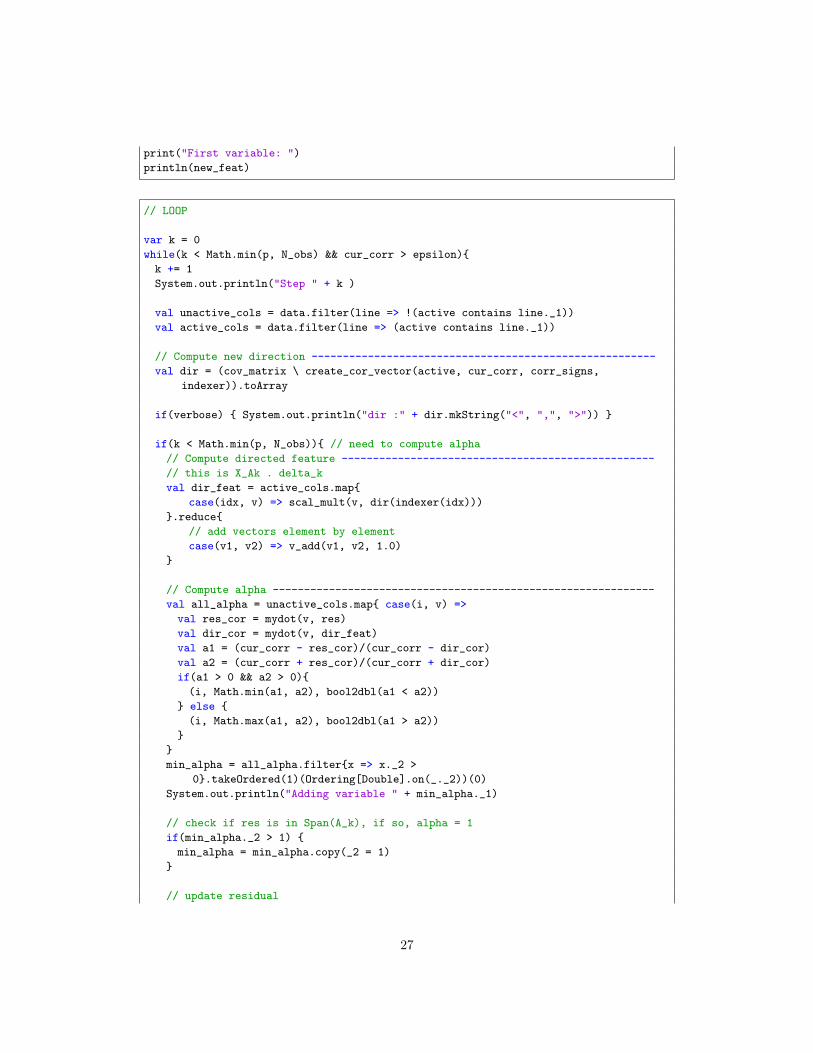
Appendix: Code sample

The full Databricks notebook is available at http://bit.do/dlars_databricks.

// INIT

// Normalize data --------------------------------------------------------------

val data = data0.map{case(idx, col) =>

val m = col.sum / col.length

(idx, col.map{v => v - m})

}.map{case(idx, col) =>

val std = Math.sqrt(col.map{v => v*v}.sum)

(idx, col.map{v => v / std})

}.cache()

// Useful variables ------------------------------------------------------------

// nb of features

val p = data.count().toInt

// nb of observations

val N_obs = labels.length

// definition of ’zero’

val epsilon = 1e-10

// control prints

val verbose = true

// Init residuel --------------------------------------------------------------

val mean_labels = labels.sum / labels.length

var res = labels.map{v => v - mean_labels}

//var vec_res = Vectors.dense(res)

var coefs = List(Array.fill(p)(0.0))

// Find first variable to add, which maximizes correlation with res ------------

val max_corr = data.map{case(idx, v) =>

val corr = mydot(v, res)

(idx, Math.abs(corr), corr)

}.takeOrdered(1)(Ordering[Double].reverse.on(_._2))(0)

// idx of the next variable to add

var new_feat = max_corr._1

// current correlation btw active set and residuel

var cur_corr = max_corr._2

// indices of the variables in the active set

var active = TreeSet(new_feat)

// init variable for later, suppose to hold (idx, alpha)

var min_alpha = (0, 0.0, 0.0)

var corr_signs = Array.fill(p)(0.0)

corr_signs(new_feat) = bool2dbl(max_corr._3 > 0)

var indexer = Map((new_feat, 0))

// init covariance matrix, its diagonal has only ones

var cov_matrix = breeze.linalg.DenseMatrix.eye[Double](1)

26

print("First variable: ")

println(new_feat)

// LOOP

var k = 0

while(k < Math.min(p, N_obs) && cur_corr > epsilon){

k += 1

System.out.println("Step " + k )

val unactive_cols = data.filter(line => !(active contains line._1))

val active_cols = data.filter(line => (active contains line._1))

// Compute new direction -------------------------------------------------------

val dir = (cov_matrix \ create_cor_vector(active, cur_corr, corr_signs,

indexer)).toArray

if(verbose) { System.out.println("dir :" + dir.mkString("<", ",", ">")) }

if(k < Math.min(p, N_obs)){ // need to compute alpha

// Compute directed feature --------------------------------------------------

// this is X_Ak . delta_k

val dir_feat = active_cols.map{

case(idx, v) => scal_mult(v, dir(indexer(idx)))

}.reduce{

// add vectors element by element

case(v1, v2) => v_add(v1, v2, 1.0)

}

// Compute alpha -------------------------------------------------------------

val all_alpha = unactive_cols.map{ case(i, v) =>

val res_cor = mydot(v, res)

val dir_cor = mydot(v, dir_feat)

val a1 = (cur_corr - res_cor)/(cur_corr - dir_cor)

val a2 = (cur_corr + res_cor)/(cur_corr + dir_cor)

if(a1 > 0 && a2 > 0){

(i, Math.min(a1, a2), bool2dbl(a1 < a2))

} else {

(i, Math.max(a1, a2), bool2dbl(a1 > a2))

}

}

min_alpha = all_alpha.filter{x => x._2 >

0}.takeOrdered(1)(Ordering[Double].on(_._2))(0)

System.out.println("Adding variable " + min_alpha._1)

// check if res is in Span(A_k), if so, alpha = 1

if(min_alpha._2 > 1) {

min_alpha = min_alpha.copy(_2 = 1)

}

// update residual

27

res = v_add(res, dir_feat, - min_alpha._2)

}

else {

// this is the last iteration

min_alpha = (0, 1.0, 0.0) // min_alpha._1 does not exist for the last iteration

}

// update coefs values

val cur_coefs = Array.fill(p)(0.0)

for(i <- active){

// coefs(0) is the last value of the coef vector

cur_coefs(i) = coefs(0)(i) + min_alpha._2 * dir(indexer(i))

}

// save coefs

coefs = cur_coefs :: coefs

if(verbose){ System.out.println(cur_coefs.mkString("<", ",", ">")) }

if(verbose) { System.out.println("Alpha step: " + min_alpha._2 + "\n") }

if(k < Math.min(p, N_obs)) {

// update for next step

new_feat = min_alpha._1

cur_corr = (1 - min_alpha._2 ) * cur_corr

corr_signs(new_feat) = min_alpha._3

// Update covariance matrix ----------------------------------------------------

val new_feat_val = data.filter(_._1 == new_feat).collect()(0)

val new_entries = active_cols.map{

case(idx, v) => (indexer(idx), mydot(v, new_feat_val._2))

}.collect().sortWith(_._1 < _._1).map{case(i,v) => v}

val vec1 = new breeze.linalg.DenseMatrix(new_entries.length, 1, new_entries)

val vec2 = new breeze.linalg.DenseMatrix(1, new_entries.length+1, (new_entries

:+ 1.0))

cov_matrix = breeze.linalg.DenseMatrix.horzcat(cov_matrix, vec1)

cov_matrix = breeze.linalg.DenseMatrix.vertcat(cov_matrix, vec2)

active = active + new_feat

indexer += (new_feat -> k)

}

}

28