Dissipative Two-Four Methods for Time-Dependent … OF COMPUTATION, VOLUME 30, NUMBER 136 OCTOBER 1976, PAGES 703-723 Dissipative Two-Four Methods for Time-Dependent Problems By David

MATHEMATICS OF COMPUTATION, VOLUME 30, NUMBER 136

OCTOBER 1976, PAGES 703-723

Dissipative Two-Four Methods for

Time-Dependent Problems

By David Gottlieb and Eli Türkei*

Abstract. A generalization of the Lax-Wendroff method is presented. This generaliza-

tion bears the same relationship to the two-step Richtmyer method as the Kreiss-

Oliger scheme does to the leapfrog method. Variants based on the MacCormack

method are considered as well as extensions to parabolic problems. Extensions to

two dimensions are analyzed, and a proof is presented for the stability of a Thommen-

type algorithm. Numerical results show that the phase error is considerably reduced

from that of second-order methods and is similar to that of the Kreiss-Oliger method.

Furthermore, the (2, 4) dissipative scheme can handle shocks without the necessity

for an artificial viscosity.

I. Introduction. Several authors (e.g. Roberts and Weiss [18], Crowley [3],

Kreiss and Öliger [9], Gerrity, McPherson and Polger [6]) have suggested that one

does not always have to treat the space and time dimensions in an equal manner even

for hyperbolic problems. This is reasonable for problems with large spatial gradients

but a slow variation in time. An example of such behavior is a stiff system where the

fastest sound speeds are of marginal significance. Since it is these sound speeds that

determine the step size, the physically important parameters will not vary much over

a few time steps. Another area of application is to problems where one is only

interested in the steady state solution. In addition they stress that halving the mesh

spacing multiplies the time by 2d+x for a ¿/-dimensional problem.

Most higher-order methods are constructed using the method of lines. In this

method one replaces the space derivatives by an approximation usually of at least

fourth-order accuracy. The resulting differential-difference equation is then solved by

a standard routine. Frequently the time derivatives are replaced by a leapfrog

approximation (see, however, Gazdag [5] and Wahlbin [23]) which leads to energy

conserving methods. However, it is frequently desirable to use dissipative methods.

The major advantage of dissipative schemes is that they are more robust than non-

dissipative methods, i.e. they are less sensitive to a variety of disturbances. The

dissipative methods are less likely to suffer from nonlinear instabilities (see Fornberg

[4] ). The spread of boundary errors into the interior is more serious for nondissipa-

tive methods especially in multidimensional problems (Kreiss and Öliger [10]). It is

also impossible to integrate equations with imbedded shocks unless the approximations

contain some artificial viscosity. Kreiss and Öliger [10] suggest adding an artificial

Received November 6, 1975.

AMS (MOS) subject classifications (1970). Primary 65M05.

"This paper was prepared as a result of work performed under NASA Grant NGR 47-

102-001 and Contract Number NAS1-14101 while the authors were in residence at ICASE,

NASA Langley Research Center, Hampton, Virginia 23665.

Copyright © 1976. American Mathematical Society

703

License or copyright restrictions may apply to redistribution; see http://www.ams.org/journal-terms-of-use

704 DAVID GOTTLIEB AND ELI TURKEL

viscosity term to the leapfrog-type schemes. Here we choose the alternative approach

of using a method which is inherently dissipative. In the results section we will

compare these two approaches.

The schemes considered in this paper are two-step generalizations of the Lax-

Wendroff method. Both Richtmyer-type and MacCormack-type multistep methods

are considered. These algorithms thus have the additional advantage that they are

minor modifications of the standard two-step methods so that existing codes using

such methods as modified Richtmyer, Thommen or MacCormack can be improved to

give fourth-order accuracy in space with a -minimum of programming. We shall first

discuss hyperbolic systems and later extend this to include parabolic terms.

II. One-Dimensional Hyperbolic Problems. We consider the following one-

dimensional divergence equation

(2.1a) «r=/*+S

or

(2.1b) ut=Aux+S

where / and S are vector functions of u, x and t and A is a matrix function of u, x, t.

In addition we shall assume that A has real eigenvalues and can be uniformly diagonal-

ized. We shall construct a finite-difference approximation only to the divergence

equation (2.1a); however, the generalization to the quasi-linear equation (2.1b) is

straightforward.

We wish to construct a finite-difference approximation to (2.1a) which is fourth-

order in space and second-order in time. Before proceeding we need to define this a

little more precisely. Kreiss and Öliger [10] define a scheme to be of order (p, q)

if the truncation error has the form

(2.2) (Ar) • 0((Atf + (Ax)").

This definition is fine for leapfrog-type methods. However, for more general schemes

all combinations of the form (Ar)'(Ajc)m can appear in the truncation error, not just

those that occur in formula (2.2). Hence, we shall generalize the definition and call

a scheme of order (p, q) if the truncation error has the form

E = Ath(At, Ax),

h = 0((Ax)q + x) whenever Ar = 0((Ax)qlp).

For the special case h — (At)P + (Ax)q this definition agrees with that of Kreiss and

Öliger.

With this definition in mind we consider the following family of schemes

<++l% - i|K+1 + <) - ¿K+2 + Hfx)

(2.4a) + aX [(, + ̂ (fn+i -f?) - £0-^ -/;Li)l + °fiS«+i + S»),


DISSIPATIVE TWO-FOUR METHODS 705

W? + X w"+ X[¿â/2 ~f"i2) + ^¿T^ ~f"-x)

(f?+2 - f]-2)\(2.4b) +3 8a

96a

?+i+*^' "cn + Oi j_ en + a

Here, /"•" = f(wf), X = At/Ax and a, a are constants. It is readily checked, by a

Taylor series expansion, that this scheme is second-order accurate in time and fourth-

order accurate in space for all a, a (a j= 0) for both linear and nonlinear

equations with sufficiently smooth solutions. That is, the local error is

0(At[(Ax)4 + (At)(Ax)2 + (Ar)2]). The amplification matrix associated with this

approximation is

(2.5) G(Ç) = / + -—p-M4 - cos£) - tiX2A2(l - cos £)(2 + a - ocos£).

We note that G is independent of a. However, for nonlinear problems a can affect

the solution (see McGuire and Morris [14]).

Since we have assumed that the matrix A is diagonalizable, the von Neumann

condition is both necessary and sufficient for stability. It is readily checked that if

g is an eigenvalue of G and "a" a corresponding eigenvalue of A, then

\g I2 = 1 - XV(1 - cos I)2 {ff - | + |(1 - cos {) + i(l - cos Ï)2

(2.6)

- (Xa)2 [l + o(l - cos Ç) + |2(1 - cos |)2]} ;

and so the stability condition is given by

1 ^80--+-X +

(2.7a) (\a)2 < mino<x<i (l + ox)2

For o not in the interval ((1 + y/vf)l6, (- 1 + \/Í3)/3) (about (.853, .868)) the

stability condition becomes

(2.7b) (Xfl)2<min(a"l>r+T)

For (1 + y/\7)¡6 < a < (— 1 + \/l3)l3 the allowable time step is marginally less

than that given by (2.7b). Thus, a practical sufficient condition is that the scheme

is stable if

(2.7c) (Xa)2 < .99 min (o - j, jÂ .

For example, if o < 1/3 the scheme is unconditionally unstable while if a = 1, we

require that \Xa | < \/2/2. The largest time step is allowed when a = (- 1 + \/l3)l3

in which case (Xa)2 < (- 2 + \/l3)/3 or \Xa \ < .731. This is very slightly larger than

that allowed by the Kreiss-Oliger scheme which permits | Xa | < .728.

The family of schemes given by (2.4) is of the Richtmyer type of two-step



methods. It is also possible to construct a scheme within the spirit of MacCormack

methods [13] :

wj1) = wf + X[rfj+2 + (1 - 2r)//+1 + (t - iy¡\ + (Arty,

wf+x = kWj + vf)) + |[(1 - r)/f> + (2t - \)ffl¡ - Tf,._2](2.8) "7 ~ 2

_X2 (' + fV/H-2 - 24+i + 2//-1 -/,-2] + f 5/1}-

For linear problems with constant coefficients this again is a (2,4) scheme for all t.

In fact the amplification matrix is again given by (2.5) if we identify

(2.9) a = - 4r(l - r); r = 14(1 ±\/l + a).

For variable coefficients the truncation error has the form

E = Ar[- Ht + ^(^/^(AxXAr) + 0((Ax)4) + 0((Ar)(Ax)2) + 0((At)2)].

The scheme given in (2.8) has a variant defined by using backward differences in the

first step and forward differences in the second step. The choice of r = - Vi allows a sta-

bility condition of X^ < H and is a (2,4) scheme. For r =£ - Vi alternating these two

variants at successive time levels will cancel the (Ar)2(Ax) error and yield a (2,4) scheme

even for variable coefficients.

For the special case t = - 1/6 (a = 7/9) this general family reduces to a scheme

that is similar to the original MacCormack scheme. In this case (2.8) reduces to

(2.10)

wf > = wf + |e//+a + 8//+1 - 7/,) + (Af)S,,

v; + 1 =|(w/ + w}1)) + ^(7/<1)-8/;P> +/#) + f.

Therefore, it would be easy to modify a code using the MacCormack scheme to be of

higher order. This method is stable when X/l < 2/3. Furthermore, for problems with

second derivatives (e.g. Navier-Stokes) the extra mesh points are needed anyway and

no new complications arise (see Section 3).

The MacCormack-like method, (2.10), has the advantage that fewer arithmetic

operations are required than for the generalization of the Richtmyer method (2.4).

Although the leapfrog and Kreiss-Oliger methods require the least amount of compu-

tations, the addition of an artificial viscosity reduces the apparent speed advantages.

In the introduction we have discussed some of the advantages of schemes that are

inherently dissipative. Lerat and Peyret [12] have shown that the post shock

oscillations can be reduced by choosing the proper variant of the MacCormack scheme.

One would expect that the appropriate variant of the MacCormack-like (2, 4) method

would have similar properties.

Since both (2.4) and (2.8) have the same amplification matrix we can discuss

both schemes (at least for linear problems) simultaneously. We shall therefore restrict

discussion to formula (2.4) with the amplification matrix given by (2.5). The corre-

spondence for the MacCormack-like (2,4) scheme is then given by (2.9).



For many problems the point of importance is not the amplitude of the waves

but their velocity. Hence, it is important to analyze the phase errors that occur by

replacing the differential equation by a difference equation. In fact this will be the

major advantage of higher-order accurate (in space) schemes. Equation (2.6) shows

that the dissipation of the (2,4) method is approximately the same as for the Richtmyer

(2, 2) method. However, the phase error of the (2, 4) method can be much smaller for

sufficiently small time steps. Since the matrix A is diagonalizable we can transform

(2.1) to a system of uncoupled equations (assuming S = 0). Hence, we shall restrict

our attention to a single scalar equation uf + aux = 0.

In any discretization procedure we are able to approximate well only the long

waves. Thus, the phase error of the higher frequency components is of little

significance, and our main interest is for £ sufficiently small. We shall, therefore,

content ourselves with a Taylor series expansion of the phase error. We define the

relative phase error as

(2-11) Ep=(P'PA)lPA

where P is the phase of the approximation and PA is the phase of the solution to the

differential equation. Straightforward algebraic manipulations yield that the relative

phase error of the (2, 4) method is given by

(2.12) Ex = \x2a2? - -¿ [4 - 15 (a - |) X2«2 + OX4*4] ? + 0(?)..

In order to study the effectiveness of the scheme we shall compare this with the

phase error for other methods. The phase error of the Lax-Wendroff method is

(2.13) E2 = - |(1 - X2a2)%2 + ~ (1 + 5X2 - 6X4)|4 + 0(?).

The phase error of the leapfrog scheme is

(2.14) E3p = -1(1 - XV)£2 + T2f5(! - 10*2*2 + 9XV)^ + 0(|6)

while that for the Kreiss-Oliger method is

(2.15) El = \x2a2? - T^ (4 - 9XV)£4 + 0(?).

Comparing these methods we see that the leading terms of the (2, 2) schemes

are the same as are those of the (2, 4) methods, but there are differences between

the two groups. The (2, 2) schemes have a lagging phase (E < 0) while the (2, 4)

schemes have a leading phase. Of greater importance is that the coefficient of i-2 is

multiplied by X2a2 for the (2, 4) methods. Since we assume that Xa is small, this

term is negligible. Specifically, we have assumed that Ar = 0((Ax)2) = 0(%2) and

so X2a2|2 is the same order as £4. Thus, the phase error of a (2, 4) method is of

fourth order for sufficiently small Ar/Ax. It should be noted that using leapfrog

in time and infinite order in space gives a leading phase error term which is identical

to that of the (2, 4) methods. Hence, in calculating phase errors of difference schemes,

it is important to consider the time discretizations as well as the space differencing.



We conclude this section with a discussion of how to choose the free parameters

a, o (r in (2.8)). It is obvious that this choice will be determined by what one is

trying to optimize. Choosing a = 3/8 in (2.4) will minimize the computer time with-

out affecting linear stability and so was used for all the tests in the result section. The

choice of a does not affect the timing for the Richtmyer-like methods. However,

choosing r = — 1/6 does reduce the required computer time for the MacCormack-like

scheme. The importance of these timing reductions will depend on the complexity

of the flux and source terms.

An alternative approach is to choose the free parameter o to optimize some

characteristic of the scheme. For example, we may wish to choose a so as to allow

the largest possible time steps consistent with stability. We have already seen that if

0 = (- 1 + y/l3)/3, then the Courant number is approximately .731. For .83 < o <

1 the Courant number is still above .7. For many applications we wish to minimize

the amount of dissipation within the scheme. By looking at (2.6) for small £ we see

that the dissipation is reduced by choosing (Xa)2 near o - 1/3. As long as a <

(1 + \J\1)I6 we can choose (Xa)2 as close as we wish to o - 1/3 without losing

stability. Of course this applies only to scalar problems, while for vector equations

the number "a" would be replaced by the sound speed of most importance. Then

waves traveling at this speed will be only slightly dissipated while others will be

damped more sharply. Hence, if one wishes to increase the allowable time steps

while limiting the dissipation one would choose o about .83 and then choose the

time step close to the allowable limit.

In many cases small dissipation does not imply an increase in accuracy. For

example, the leapfrog and Lax-Wendroff schemes display similar L2 errors thought

their dissipative properties are quite different. Thus, in many instances we wish to

decrease the phase error rather than decrease the dissipation. As already discussed,

(2.12) implies that the relative phase error decreases as one decreases the time step.

Hence, in this instance we are no longer interested in choosing a so as to increase the

allowable time step. Instead we choose a to minimize dissipation as well as phase

errors. Thus, we choose Xa near the stability limit with Xa small. In trial experi-

ments, a Courant number of Xa = .25 yields reasonable results for one-dimensional

problems (see Öliger [16] and Abarbanel, Gottlieb and Türkei [1]). In this

particular case a choice of o = .4 would be appropriate. The graphs discussed in

the result section confirm this prediction. Thus, the family of schemes given by

(2.4) or (2.8) has the property that various features can be optimized by just

choosing the appropriate choice for the free parameter. Hence, there is more discretion

left to the user in adapting the scheme to his particular problem.

Equation (2.6) implies that the (2, 4) scheme is fourth-order dissipative in the

sense of Kreiss. This is the same order of dissipation as in the (2.2) Richtmyer

method. Choosing o and XA appropriately can reduce the coefficient of dissipation

but not the order. Thus, it is not possible to reduce the dissipation sufficiently for

many problems. A solution to this difficulty is to alternate the dissipative (2, 4)

method with the Kreiss-Oliger scheme. This composite scheme is now a three-step



method of which the first two steps are given by (2.4a), (2.4b) and the third step is

(2.4c) wy + 2 = wf + ^ [8(#.y -/;_V ) - <#+» -Z}^1)] + 2Ai5;+1.

It is readily calculated that the eigenvalues of the amplification matrix are such that

\g I2 = 1 - |x4a4(l - cos £)3(1 + cos £)(4 - cos £)

(2.6) - ia -1 + |(1 - cos |) + |(1 - cos £)2

- (Xa)2 [l + o(\ - cos |) +£ (1 - cos |)2] J .

Thus, the scheme is now sixth-order dissipative for long wave lengths while |g|2 = 1

for % = it. It is obvious by comparing (2.6) with (2.16) that the stability criteria for

the two- and three-step methods are identical. Since (2.4c) does not involve many

arithmetic operations the composite three-step method will also be more efficient.

Such methods for second-order methods are described in more detail in Türkei [22].

R. Warming (private communication) showed that one can also decrease the

dissipation by considering three-step (2, 4) methods. One can also consider three-step

third-order methods in order to reduce the dissipation.

III. ParaboUc Equations. In fluid dynamic problems one is frequently interested

in extending the previous results to equations that include a small viscous term. At

high Reynolds numbers the restriction imposed by the parabolic stability condition

is comparable with the Courant condition. Furthermore, (2, 4) schemes are more

natural for parabolic equations than for hyperbolic equations.

A second-order in time explicit method for a parabolic equation in one space

dimension requires a numerical domain of dependence of at least five points at the

previous time step. Thus, any of the variants of the multistep (2.2) schemes require

five net points in each direction in order to advance the solution for the Navier-Stokes

equations. In principle a (2, 4) method should not require any more points and so

one would increase the accuracy of the solution without complicating the problem.

From (2.4a) it is seen that the first step of the Richtmyer-like (2, 4) method

requires information at the four points / — 1, /, / + 1, / + 2. Since an evaluation of

second derivatives at the second step requires at least three points, it follows that this

method requires at least seven points in order to have second-order accuracy in

time for the parabolic terms. Instead, we shall study generalizations of the

MacCormack-type method given by (2.8).

We consider an equation of the form

(3.1) ut = fx + (Aux)x + S.

The straightforward approach is to replace f, by ff + Af(w- - Wj_x)lAx in the first step

and fj-x) by /;(1) + Af(wj+, - w;)/Ax in the second step of Eq. (2.10). This results

in a truncation error of the order Ar [(Ax)4 + (Ar) (Ax)]. Another approach is to let



«T = wi + % I*//« + o - 2^+i + fr - »//]

+ -^-2 W/+1(",+ a - wy+,) - il/w/+ ! - Wf)] + (Ar^,

(3.2)

w« + 1 =i(W/ + w(») + ^[(l -r^>) + (2r- 1)/}!} -^1

+ -^L7K(w}1>-w(l))-^._1(w(!) -w}1))]2(Ax)2 ' ' ' ' ' '

At

12(Ax)[Af+2(wi+2 - wj+1) + Aj+l(5wj+2 - 13w/+1 + 9w;. - w,.,)

+ ^/(W/+2 ~ 13wj+l + 24wj * 13w/-l + Wj-2)

-Af_i(wf+1 - 9Wj + 13W/_, - 5w._2) -^(wî - w;._2)]

+ fs<.>As before, r is a free parameter which can be chosen to reduce the number of arith-

metic operations or to minimize the phase error of the convective part of the solution.

The truncation error behaves as

T = (At)0((Axf + (Ar)(Ax) + (Ar)2)

and for constant coefficients

T = AtO((Axf + (Ar)(Ax)2 + (Ai)2).

The above algorithm has the disadvantage that it is not a true (2,4) scheme for

nonlinear problems because of the (Ar)2(Ax) term in the truncation error. An

alternative approach is to use the Richtmyer-type method (2.4) for the convective

terms. The parabolic terms can then be incorporated by using a splitting technique

(see Strang [19], Marchuk [15]). Thus, we label the numerical procedure given by

(2.4) as L. We then follow this by using (3.2) (with /= 0) and label this procedure

as M. In general this splitting will no longer be second-order in time. However, it is

known that the most efficient procedure is to alternate the order of the operations,

i.e. at one time step to use ML and at the next time step to use LM. This procedure

does not require more operations than the combined algorithm given by (3.2). It

is now straightforward to show rigorously that the stability condition is given by the

more stringent of the hyperbolic and parabolic restrictions. It can also be shown that

this splitting preserves the (2, 4) accuracy of the method even for nonlinear problems

(see Gottlieb [8]). That is, even though only second-order splitting is used this is

necessary only to preserve the second-order accuracy in time. The fourth-order

accuracy in space is not destroyed by any splitting procedure.



It is now no longer necessary to use the same algorithm for both the convec-

tive and dissipative terms in (3.1). In many instances it is desirable to use implicit

methods for the parabolic part of the splitting. This is particularly useful when the

convective terms are nonlinear but the viscosity terms are linear. Then the implicit

parabolic part is easily in vertible and does not affect the stability criteria. The

allowable time steps will then be determined only by the convective terms.

IV. Two-Dimensional Problems. There are two ways that one can generalize the

previous results to multidimensional problems. The first is to use a splitting technique

similar to that described in the last section. This will preserve the (2, 4) accuracy of

the solution and can incorporate both the hyperbolic and parabolic components of the

equation. Another approach is a straightforward generalization of the finite-difference

equations. Here we shall only consider generalizations of the Richtmyer-type scheme

(2.4) for hyperbolic equations.

The natural extension to two space dimensions would be a generalization of the

Burstein schemes [2]. In this method the intermediate results are calculated at time

t + aAt and at the center, (i + ]/4, / + &), of the mesh cells. We shall now show

that no such two-step scheme is possible which is both (2, 4) accurate and also stable

for arbitrary symmetric hyperbolic systems.

Consider the system

(4-1) ut=fx+gy=Aux+Buy.

In order to simplify the notation we introduce the averaging and differencing opera-

tors

wi+HJ + Wi-V*,j

ß*Wy 2 ' xJi.j -fi+Vij fi+'AJ-

We then consider the general scheme of the form

w" + « = uxMJ,(l4(5* + 5*))vv

+ oa[i - ^(S2 + Ô2) + Y^26252] lW + 8„M'

(4.2) r

•»+» = w + x\ßx(8xß/"+a + 8ylixg"+a) + (ß2 + ß3n2y + ßyyy>xßxf

+ (ß2+ p>2 + ß^yßyg + (ß5+ ß6u2 + ßÂf

+ (ßs + hÂ + ßi^y^yS - \(li + T,*£)8&/

-£(7l +72M2)S>^.

= A sin | cos ^ + B sin | cos |, N = A sin | cos | + Bsin % cos ^.

w

Define

M

The amplification matrix for the linearized equations is



,2 i+sin2?

Git n) = I + 2iM 111 +-^2-~)cos |cos f

+

(4.3)

a (~1 + a, (sin21 + sin21 \ - a2 sin21 sin2 11 [

+ 2¿Wcos | cos 2 L + 204 + /3S + ]37 + 7j + 72

- (02 + ^4) (si"2 f + sin2 y + 07sin2 | sin2 |1

+■ 2irV [ß2 - ß4 + 2ßs + ß6 - n -72+034-^-136+7! + 72)

• (sin2 I + sin2 Ü\-(ßA-ß6+ 72)sin2 |sin2 |J .

When .4 and B are scalar one can choose % and n so that M = 0 but A =£ 0 and so G =

/ + /(7A which is not stable. Hence a necessary condition for stability is that q(%, n)

vanish identically for all £, tj.

Thus, we require

(1) ß2 - 04 + 2ß5 + ß6 - (7, +72) = 0,

(4-4) (2) 04 - ß5 - ß6 + 7i + 72 = 0,

(3) 04 - ß6 + 72 = 0. •

For (2, 4) accuracy we also require

(4) ß, +02 +03 +04 +05 +06 +07 =1.

(5) o0, = 1/2,(4.5) l

(6) ßx + 4(02 + 03 + 04) + 1O(0S + 06 + 07) - 6(7i + 72) = 0,

(7) 0j + 203 + 404 + 206 + 407 = 0.

A straightforward calculation shows that these equations are inconsistent and so no

scheme of the above type can be both stable and (2, 4) accurate.

As an alternative we now construct a method of the Thommen type [20]. In

this method there are two intermediate levels: one for the /flux and one for the

g flux term. The amplification matrix for the (2, 2) scheme is identical with that of

the one-step Lax-Wendroff. We, therefore, consider

-(1)=^(l-|ô2)- + |5:c(l4al524a2S2+T|a3Ô262y

+ \f>yHyVx (l - \a482x - \a582y + ±a682x82y) g,

KWy (l ~Wl -\a582y+±a662x8ty

«75x -\asdy+Jâ9^Í)g>

X5>X , *5>v

(4.6)"(2)=^(l-Í62)w+!

+KK

^- + M/) + «/«.-f/"^»



allThis scheme has order of accuracy (2, 4) for both linear and nonlinear problems for all

values of the free parameters a,.. Thus, these parameters can be chosen to improve the

stability criterion or reduce the phase error, as in the one-dimensional case. The

amplification matrix of this scheme is

G(£, T?) = / + j-X Usin |cos|(4 - cos2|) + Äsin ^ Cos |(4 - cos2r?)|

-2X2L2sin2|(l +a1sin2|+a2sin2| + a3 sin2 |sin2|\

(4.7) + 52sin2| il +a7sin2| + a8sin2^ + a9sin2|sin22\

+ (AB + BA)sm^sm^¡ cos^-2™2W"2

• cos^ [ 1 + a\ (l +cv4sin2| +assin2| + a6sin2f sin2f)].

It is exceedingly difficult to find a stability criteria for general matrices A and B

as a function of the nine free parameters. We shall therefore only obtain an analytic

stability condition under the assumption that

n 2 4a2=cx3=a1=cx9 = 0, a4=as=-, %=-,

(4.8)

a, = a8 = a (= arbitrary).

In this case the amplification matrix can be written as

where

GQi, V) = I + 2iN - 2(N2 + cX2A2 + dX2B2),

p = cosí-, q = cos^,

N=XAp(l +|p2Wl-p2 + Xß<?(l +!<72Vl -q2,

c=P4(a-|+|p2+|p4), , = ,4(a-|+f,2+^).

A sufficient condition for stability is |(Gu, u) | < 1 for all unit vectors u (see [11]).

Let n — \Nu \, a = \Au |, and b = \Bu\. For symmetric matrices A, B we have

|(Gu, u)|2 = 1 - 4(n2 + ca2 + db2) + 4(n2 + ca2 + db2)2 + 4(Au, u)2

(4.9)< I - 4(«2 + ca2 + db2) + 4(«2 + ca1 + db2)2 + 4«2.

Hence, a sufficient condition for stability is that

(4.10) (n2 + cX2a2 + dX2b2)2 < X2(ca2 + db2),

but



n2 < 2X2 |a2p2 (l + ¡p2) 2(1 - p2) + b2q2 (l + \q2} \\ - q2)~\,

(n + cX2a2 + dX2b2)2

<2X2j2[a2p2(l+|p2y(l-p2)]

+ ca2 + 2 [è V (l + \q2\ (1 - ç2)] + db2\ .

Substituting this back into (4.10) and using the definitions of c and d we find that a

sufficient condition for stability is that

8XV(l+^«+iy-|p*+|p*)a+8XV(l+i(a + |y-|^-|^) =

3+9P V;+X*T 3 +9* 9*

We assume that a > 1/3 so that a > Vi(a + 1/3), and

l+^(a + f)p2-4p4-!p'<l+aV.

Thus, a sufficient condition is that

8X4a4(l + op2)2 + 8X4Z>4(1 + aq2)2

<xv(a-|+fp2+^)+x2Ä2(a-i+|<72+|iZ4).

Taking each part separately, a sufficient condition for stability is that

(4.11) 8(Xa)2 < min-°<P<! (1+ap2)2

and a similar condition for Xb. However, comparing (4.11) with (2.7a) we notice that

the expression on the right-hand side of (4.11) is exactly the same as appears in the one-

dimensional case. Hence, a sufficient condition for stability is that Xa and Xb be

reduced by a factor of l/y/& from that required in the one-dimensional case So from

(2.7c) we have that a sufficient condition for stability is that

.99 . / 1 1(4.12) 0)2<^min(cY-^, rh) and (**)2<t-min(a-f'TT^)-3' 1 +

For a more general choice of parameters than that given in (4.8) we use numeri-

cal methods. Türkei [21] has shown that for the amplification matrix given by (4.7)

a sufficient condition for stability for real symmetric matrices A, B can be obtained by

replacing A and B by scalars.

The question of stability is now reduced to finding bounds on the scalars A, B

so that | G(£, t?) | < 1. This can be found by running computer tests with a selection


DISSIPATIVE TWO-FOUR METHODS

of scalars A and B and for a set of %, r\ between - it and ti. The results of this

computer run are given in Table I.

Table I

Sufficient stability conditions for Eq. (4.6) found by

assuming that A and B are scalars

parameters

afa8=1 «2=a3=«7=a9=0 W§

al=a2=a7=a8=1 a7=a9=0 a4=a5=3

WWW1

ai=a2=a7=a8=l

a3=a6=a9=0

a3=a4=a5=a6=a9=0

"6 9

a6=9

stability condition

A2/3+ B2/3 ̂ jfáz ?9

A2 + B2 <I

A2 +B2 <\

A2/3+ B2/3 < .68

V. Numerical Results. Two model problems were chosen to compare several

methods. These problems contain the main features of hyperbolic systems: wave

propagation and shocks. The first problem is a scalar constant coefficient equation

ut + ux = 0,

(5.1)

with an initial condition

0<x<°°, 0 < í < 10,

u(x, 0) = f(x),

0, 0<x<l,

f(x) = j sin (8tt(x - 1)), 1 < x < 2,

0, 2 < x < °°.

The solution is just a wave moving to the right: u(x, t) = f(x - t). The numerical

domain of integration is chosen sufficiently large so that the boundaries do not

influence the solution for 0 < t < 10. Figure 1 shows the solution at t = 10 using

the two-step Richtmyer method with Ax = 1/40 and At I Ax = .9. Figure 2 shows

the solution using the (2,4) scheme (2.4) with a = 3/8, a = 0.4 and At/Ax = .25.

Figure 3 shows the solution given by the Kreiss-Oliger scheme with Ax = 1 /40 and

At j Ax = .25. Finally in Figure 4 we show the results obtained by alternating the

(2.4) method (o = 1.0) and the Kreiss-Oliger scheme as described in Section 2. From

these graphs we see that the phase error of the (2.4) dissipative scheme is considerably

better than that of the Richtmyer method and is comparable with Kreiss-Oliger. For

the set of parameters chosen, the scheme (2.4) possesses much less dissipation than

the Richtmyer method. The composite dissipative (2,4)—Kreiss-Oliger scheme also

gives good results.



Figure 1

The second problem is that of a shock wave for the fluid dynamic equations

pt + (pu)x = 0, (pu)t + (pu2 + p)x =0, Et+ [u(E + p)]x= 0,

(5.2)

E = p(e + lAu2); p = (y - \)pe,

with the initial conditions

x<0 x>0

p = 2.5 p = 1

u = .6 + y/5 u = 1

p=4 p=l

These conditions correspond to a relatively strong shock.

The results show that it is feasible to use the dissipative (2, 4) method on

shocks without adding an artificial viscosity. Choosing time steps near the stability

limit produces small overshoots. This is seen in Figure 5 for the Lax-Wendroff

scheme with a CFL = .9 and in Figure 6 for the (2, 4) method with a = 3/8, a = 1

and CFL = .7. Here CFL is defined as Ar/Ax( |u | + c). Notice that for the (2, 4)



Figure 2

scheme the major overshoot is in front of the shock for both methods. As expected,

decreasing a decreases the dissipation of the method and so enlarges the oscillations.

For the first problem (5.1) we choose a = .4 to reduce the dissipation while we now

choose a = 1 to increase the dissipation. In more realistic problems it may be possible

to choose a as a function of the gradients so as to increase the dissipation only in the

neighborhood of the shock.

Figures 7 and 8 show the leapfrog and the Kreiss-Oliger schemes, respectively,

using an additional viscosity as given by Kreiss and Öliger [10]. We chose a viscosity

coefficient of 1.0; choice of a smaller viscosity led to large post shock oscillations.

This large viscosity coefficient required the use of a smaller time step, CFL = 0.75, for

the leapfrog method while the Kreiss-Oliger method was run with CFL = 0.5. Figure 9

shows the Kreiss-Oliger method with a viscosity of 0.1 and CFL = 0.5 (choice of a

smaller time step only slightly reduced the oscillations). The use of these parameters

is not desirable for a smooth problem. Reducing the time step for the leapfrog method

increases the phase error. A reduction from CFL = 0.9 to CFL = 0.75 increased the

phase error by about 30% while a further reduction to CFL = 0.25 rendered the

solution meaningless. Thus, the smaller time step required by the viscosity terms in

the leapfrog method affects the accuracy for smooth problems as well as increasing

the running time. The use of such large viscosity coefficients also causes a large energy



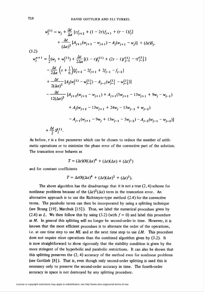
Figure 3

loss for smooth regions. Figure 10 shows the traveling wave problem Eq. (5.1) when

solved by the Kreiss-Oliger scheme with a viscosity of 1.0 and CFL = 0.25. This

should be compared with Figure 3 which shows the solution obtained with the same

scheme but without any viscosity. Any attempt to use time steps near the stability

limit is disastrous for the Kreiss-Oliger method. From the above we see that when a

problem contains both smooth and shocked regions it will be difficult to choose a viscos-

ity coefficient for either the leapfrog or Kreiss-Oliger methods that will yield acceptable

solutions in all regions. A similar phenomena occurs in the dissipative (2, 4) scheme

where the choice of o is different for the smooth and shocked regions.

The Richtmyer method required about 5.9 seconds of CPU time to achieve the

solution for the shock problem shown in Figure 5. The leapfrog method viscosity

required 3.6 seconds. The (2, 4) dissipative scheme with CFL = 0.7 needed about 9.9

seconds while the Kreiss-Oliger method with viscosity and CFL = 0.50 used 7.6 seconds.

All programs were run on a CDC 6600 KRONOS system at NASA Langley. The leap-

frog type programs require about twice as much storage as do the multistep methods.

Had the two-step methods been programmed to use two storage levels rather than one,

a substantial time savings would have been realized.


DISSIPTIVE TWO-FOUR METHODS 719

:,1

.7-

co ■«■x c '.cr ,af

=> A

.3

.2

.]

fX* X X x

3g x 3.60 3.82 JO-OH 1

x-.1

.2

.3

.4

.5

.6

.7

.8

.3

1.0

x*x

x x

');'\ '.âk5B

Figure 4

OT^

-I-1-1-1-4- -i-1-1-1- -4-I-1-1-t-

-1.00 -.17 -.5t .31 -.09 .mX AXIS

.31 .60

Figure 5



£f

-I-1-I-1-1-1-1-1-1-1-1-4--1.00 -.11 -.5» .31 -.09

X RXIS

-i-1-)-1-

FlGURE 6

07

-t-1-1~ -t-1-1--t-1-(-1-1-4-3-1.00 -.11 -.5« .31 -.09 .11

X RXIS60

Figure 7

2'.50

2.25

2.00

1.75

>-1.53

to 1.25

Si.DO.75-

.50 —

.25 —

-oUlX AXIS

-.6 -.1 -.2 0 .2

T~" I.a i -o

Figure 8



2-50

2.25

2.00

1 .75

>-l .50h-

11.00-,75

.50

.25

-0 .0 -.8

'MrAAA^yi

X AXIS.2 0 .2

r_

1.0

Figure 9

1-0

.3 —

■B-r

.7 —

, .B —

CE -ö

=> .4

.3

.2

.1

.2

.3

.4

.5

.B

.7

.B

.9

1 .0

^^^«^^-¿^m.^^^Lü<*x

14 li-38^ I1.5RÄ-*xxxxi

FlGU*E 10



VI. Conclusions. A two-step method is constructed which is fourth-order in space

and second rder in time. The method can be constructed as a generalization of either

Richtmyer r MacCormack-type schemes. There is a free parameter, a, which can be

chosen to emier allow larger time steps or else change the inherent dissipation of the

scheme or to improve the velocity of the solution. It is found that phase error is

sharply reduced by choosing relatively small time steps, about a quarter of the Courant

condition, rather than near the stability limit. Choosing o = 0.4 and a Courant number

of 0.25 gives very good phase resolution with little dissipation. For problems with large

gradients choosing o = 1.0 decreases the oscillations.

Comparisons, in one dimension, are made with second-order methods and with

the Kreiss-Oliger method. The phase error for the (2, 4) methods is much smaller

than for (2, 2) schemes. Analysis indicates that the phase error for (2, °°) methods

are about the same as for (2, 4) methods. For a shock problem very high viscosities

are required for the leapfrog and Kreiss-Oliger methods to prevent violent post shock

oscillations. This required the use of smaller time steps for the leapfrog method. The

use of this large viscosity for smooth problems gives large energy losses. Furthermore,

decreasing the time steps greatly increases the phase error for the (2, 2) methods

while decreasing the phase error for the (2, 4) methods. These problems will create

difficulties for calculations that contain both smooth and shocked regions. Boundary

treatment of the dissipative (2, 4) scheme is being presented by Goldberg [7].

Since the dissipative (2, 4) method uses five points at the previous time step (in

one dimension) it is possible to generalize the MacCormack-type method to include

parabolic terms without increasing the domain of dependence. It is then necessary to

alternate the order of the one-sided difference steps to preserve the fourth-order

accuracy in space.

In two space dimensions it is shown that one cannot construct a stable Burstein

type (2, 4) method. As an alternative, we construct a Thommen-type scheme. An

analytic stability condition is derived for one set of the free parameters while other sets

are calculated numerically.

Numerical results are presented for one-dimensional smooth and shocked flows.

Acknowledgement. The authors wish to thank Dr. R. Warming for his fruitful

comments. (2.10) was found by him independently.

Institute for Computer Applications in Science and Engineering

NASA Langley Research Center

Hampton, Virginia 23665

Courant Institute of Mathematical Sciences

New York University

251 Mercer Street

New York, New York 10012

1. S. ABARBANEL, D. GOTTLIEB & E. TURKEL, "Difference schemes with fourth order

accuracy for hyperbolic equations," SIAMJ. Appl. Math., v. 29, 1975, pp. 329—351.

2. S. Z. BURSTEIN, "High order accurate difference methods in hydrodynamics," Nonlinear

Partial Differential Equations, W. F. Ames, Editor, Academic Press, New York, 1967, pp. 279-290.

MR 36 #510.



3. W. P. CROWLEY, "Numerical advection experiments," Monthly Weather Review, v. 96,

1968, pp. 1-11.

4. B. FORNBERG, "On the instability of leap-frog and Crank-Nicholson approximations of

a nonlinear partial differential equation," Math. Comp., v. 27, 1973, pp 45—57.

5. J. GAZDAG, "Numerical convective schemes based on accurate computation of space

derivatives,"/. Computational Phys., v. 13, 1973, pp. 100-113.

6. J. P. GERRITY, JR., R. P. McPHERSON & P. D. POLGER, "On the efficient reduction

of truncation error in numerical prediction models," Monthly Weather Review, v. 100, 1972,

pp. 637-643.

7. M. GOLDBERG. (To appear.)

8. D. GOTTLIEB, "Strang-type difference schemes for multidimensional problems," SIAM

J. Numer. Anal., v. 9, 1972, pp. 650-661. MR 47 #2826.

9. H.-O. KREISS & J. ÖLIGER, "Comparison of accurate methods for the integration of

hyperbolic equations," Tellus, v. 24, 1972, pp. 199-215. MR 47 #7926.

10. H.-O. KREISS & J. ÖLIGER, Methods for the Approximate Solution of Time Dependent

Problems, Global Atmospheric Research Programme Publications Series, no. 10, 1973.

11. P. D. LAX & B. WENDROFF, "Difference schemes for hyperbolic equations with

high order of accuracy," Comm. Pure Appl. Math., v. 17, 1964, pp. 381-398. MR 30 #722.

12. A. LERAT & R. PEYRET, "Noncentered schemes and shock propagation problems,"

Internat. J. Comput. & Fluids, v. 2, 1974, pp. 35-52. MR 50 #15586.

13. R. W. MacCORMACK, Numerical Solution of the Interaction of a Shock Wave with a

Laminar Boundary Layer, Proc. 2nd Internat. Conf. on Numerical Methods in Fluid Dynamics

(M. Holt, Editor), Springer-Verlag, Lecture Notes in Phys., vol. 8, 1970, pp. 151-163.

MR 43 #4216.

14. G. R. McGUIRE & J. LI. MORRIS, "A class of second-order accurate methods for the

solution of systems of conservation laws," /. Computational Phys., v. 11, 1973, pp. 531—549.

MR 48 #10140.

15. G. I. MARCUK, "On the theory of the splitting-up method," Numerical Solution of

Partial Differential Equations, II (SYNSPADE 1970), B. Hubbard, Editor, (Proc. Sympos., Univ. of

Maryland, College Park, Md., 1970), Academic Press, New York, 1971, pp. 469-500.

MR 44 #1234.

16. J. ÖLIGER, "Fourth order difference methods for the initial boundary-value problem

for hyperbolic equations," Math. Comp., v. 28, 1974, pp. 15-25. MR 50 #11798.

17. R. D. RICHTMYER & K. W. MORTON, Difference Methods for Initial-Value Problems,

2nd ed., Interscience Tracts in Pure and Appl. Math., no. 4, Interscience, New York, 1967.

MR 36 #3515.

18. K. V. ROBERTS & N. O. WEISS, "Convective difference schemes," Math. Comp., v. 20,

1966, pp. 272-299. MR 33 #6857.

19. G. W. STRANG, "On the construction and comparison of difference schemes," SIAM

J. Numer. Anal., v. 5, 1968, pp. 506-517. MR 38 #4057.

20. H. U. THOMMEN, "Numerical integration of the Navier-Stokes equations," Z. Angew

Math. Phys., v. 17, 1966, pp. 369-384. MR 34 #5387.

21. E. TURKEL, "Symmetric hyperbolic difference schemes," Linear Algebra and Appl.

(To appear.)

22. E. TURKEL, "Composite methods for hyperbolic equations," SIAM J. Numer. Anal.

(To appear.)

23. L. B. WAHLBIN, "A dissipative Galerkin method for the numerical solution of first

order hyperbolic equations," Mathematical Aspects of Finite Elements in Partial Differential Equations

(Proc. Sympos., Univ. of Wisconsin, C. de Boor, Editor), Publ. No. 33 of the Mathematics

Research Center, Univ. of Wisconsin, Academic Press, New York, 1974, pp. 147-169. MR 50

#1525.


Documents

Dissipative Two-Four Methods for Time-Dependent … OF COMPUTATION, VOLUME 30, NUMBER 136 OCTOBER 1976, PAGES 703-723 Dissipative Two-Four Methods for Time-Dependent Problems By David