DISSERTATION

SIMULATING SOUTHWESTERN U.S. DESERT DUST INFLUENCES ON SEVERE,

TORNADIC STORMS

Submitted by

David Gregory Lerach

Department of Atmospheric Science

In partial fulfillment of the requirements

For the Degree of Doctor of Philosophy

Colorado State University

Fort Collins, Colorado

Spring 2012

Doctoral Committee:

Advisor: William R. Cotton

Steven A. Rutledge

Sonia M. Kreidenweis

Larry A. Roesner

ii

ABSTRACT

SIMULATING SOUTHWESTERN U.S. DESERT DUST INFLUENCES ON SEVERE,

TORNADIC STORMS

In this study, three-dimensional numerical simulations were performed using the

Regional Atmospheric Modeling System (RAMS) model to investigate possible

southwestern U.S. desert dust impacts on severe, tornadic storms. Initially, two sets of

simulations were conducted for an idealized supercell thunderstorm. In the first set, two

numerical simulations were performed to assess the impacts of increased aerosol

concentrations acting as cloud condensation nuclei (CCN) and giant CCN (GCCN).

Initial profiles of CCN and GCCN concentrations were set to represent “clean”

continental and aerosol-polluted environments, respectively. With a reduction in warm-

and cold-rain processes, the polluted environment produced a longer-lived supercell with

a well-defined rear flank downdraft (RFD) and relatively weak forward flank downdraft

(FFD) that produced weak evaporative cooling, a weak cold-pool, and an EF-1 tornado.

The clean environment produced no tornado and was less favorable for tornadogenesis.

In the second ensemble, aerosol microphysical effects were put into context with

those of CAPE and low-level moisture. Simulations initialized with greater low-level

moisture and higher CAPE produced significantly stronger precipitation, which resulted

in greater evaporation and associated cooling, thus producing stronger cold-pools at the

surface associated with both the forward- and rear-flank downdrafts. Simulations

initialized with higher CCN concentrations resulted in reduced warm rain and more

supercooled water aloft, creating larger anvils with less ice mass available for

iii

precipitation. These simulated supercells underwent less evaporative cooling within

downdrafts and produced weaker cold-pools compared to the lower CCN simulations.

Tornadogenesis was related to the size, strength, and location of the FFD- and RFD-

based cold-pools. The combined influence of low-level moisture and CAPE played a

considerably larger role on tornadogenesis compared to aerosol impacts. However, the

aerosol effect was still evident. In both idealized model ensembles, the strongest,

longest-lived tornado-like vortices were associated with warmer and weaker cold-pools,

higher CAPE, and less negative buoyancy in the near-vortex environment compared to

those storms that produced shorter-lived, weaker vortices.

A final set of nested grid simulations were performed to evaluate dust indirect

microphysical and direct radiative impacts on a severe storms outbreak that occurred

during 15-16 April 2003 in Texas and Oklahoma. In one simulation, neither dust

microphysical nor radiative effects were included (CTL). In a second simulation, only

dust radiative effects were considered (RAD). In a third simulation, both dust radiative

and indirect microphysical effects were simulated (DST), where dust was allowed to

serve as CCN, GCCN, and ice nuclei (IN). Fine mode dust serving as CCN reduced

warm rain formation in the DST simulation. Thus, cloud droplets were transported into

the mixed phase region, enhancing freezing, aggregation, and graupel and hail

production. However, graupel and hail were of smaller sizes in the DST simulation due

to reduced riming efficiencies. Dust particles serving as GCCN and IN played secondary

roles, as these impacts were offset by other processes. The DST simulation yielded the

lowest rainfall rates and accumulated precipitation, as much of the total water mass

within the convective cells were in the form of aggregates and small graupel particles that

iv

were transported into the anvil region rather than falling as precipitation. The combined

effects of warm rain efficiency, ice production, and hydrometeor size controlled the

evolution of cold-pools and storm structure. The RAD and CTL simulations produced

widespread cold-pools, which hindered the formation of long-lived supercells relative to

the DST simulation. The DST convective line was associated with reduced rainfall and

multiple long-lived supercells.

Comparisons between the RAD and CTL simulations revealed that dust radiative

influences played an important role in convective initiation. The increased absorption of

solar radiation within the dust plume in the RAD simulation warmed the dust layer over

time, which reduced the amount of radiation that reached the surface, resulting in slight

cooling at the surface and increased atmospheric stability within the lowest 2 km. Dew

points at low levels were slightly lower in the RAD simulation, due to reduced surface

water vapor fluxes (latent heat fluxes) below the dust plume. With the presence of a

stronger capping inversion but more available low-level moisture, the CTL simulation

initially produced more widespread convection and precipitation, while the RAD

simulation produced the strongest convective cores, including a long-lived supercell.

The results from all three sets of simulations suggest that dust indirect

microphysical and direct radiative impacts on severe convection may at times greatly

influence the development of severe storms. In this study, dust often increased the

potential for tornadogenesis. Additional modeling studies at horizontal grid spacing ≤100

m are needed in order to address the robustness of these results and better isolate

potential dust influences on severe storms and tornadogenesis.

v

ACKNOWLEDGMENTS

I would like to offer a humble thank you to my advisor Dr. William Cotton, for

his support, guidance, and mentorship through the last five and a half years. I would like

to thank Drs. Sonia Kreidenweis and Steven Rutledge of the Department of Atmospheric

Science at CSU as well as Larry Roesner of the Department of Civil Engineering for

participating as members on my doctoral committee. In addition, thank you to Dr. Jorge

Ramirez of Civil and Environmental Engineering for being a member on my committee

through January 2012. Dr. Kreidenweis also made significant contributions to my

research dealing with the microphysical activation of dust in RAMS. I would also like to

offer my sincerest gratitude to Steve Saleeby of CSU, who over the years gave up

countless hours of his time teaching me the intimate workings of RAMS and contributed

many ideas that were implemented into RAMS as part of this study. Thanks to all past

and present members of the Clouds and Storms research group. Specifically, Dan Ward

helped with the parcel simulations that resulted in the dust-CCN lookup table used in this

work. He also provided the WRF/Chem output that was utilized in the 15-16 April case

simulations. My office mate Adrian Loftus provided many thought-provoking

conversations on deep convection.

I’d like to acknowledge Drs. Sue van den Heever of CSU, Brian Gaudet of PSU,

and Louie Grasso of CIRA, who provided thoughtful insight to various aspects of this

work. Dr. Gaudet also performed the initial idealized aerosol simulations presented in

Chapter 4. I want to thank Dr. Thomas Gill of UTEP, who showed great interest in this

work and provided various references and data sources regarding southwestern U.S.

desert dust. Dr. Steven Miller of CIRA performed an advanced dust detection algorithm

vi

on MODIS satellite data to identify lofted dust in the 15-16 April case study, and Dr.

Daniel Lindsey of CIRA provided formatted GOES satellite data files for the same case.

Paul DeMott of CSU provided helpful clarification regarding the use of his

heterogeneous ice nucleation scheme. Both Dr. Brian McNoldy and Nick Guy of CSU

aided in IDL visualization. I would also like to thank the late Ed Danielson for providing

the initial motivation for this study. This work was funded by National Science

Foundation (NSF) Grant ATM-0638910.

Most importantly, I need to express my sincerest thanks to my family, God, and

all of my friends for their never-ending love and support. I would not be where or who I

am today without you.

vii

TABLE OF CONTENTS

1. Introduction ……………………..………………………………………………........1

1.1 Motivation ...…………………………………………………….....................1

1.2 Objectives and Methods ...……………………………………………............4

2. Background ……………………………………………………………………….….9

2.1 The Supercell ……………………………………………………………..…..9

2.1.1 Environmental Factors ………………………………………….......9

2.1.2 Supercell Characteristics ………………………………………….11

2.1.3 Sources of Rotation ……………………………………………….16

2.2 Tornadoes and Tornadogenesis ……………………………………………..21

2.2.1 Nonsupercell Tornadogenesis ………………………………….….22

2.2.2 Supercell Tornadogenesis ………………………………………....23

2.2.2.1 The Dynamic Pipe Effect ……………………………….24

2.2.2.2 Role of the FFD …………………………………………26

2.2.2.3 Role of the RFD ………………………………………....26

2.2.2.4 Barotropic Mechanisms …………………………………32

2.2.2.5 Frictional Effects ………………………………………..33

2.3 Cloud Nucleation Theory ………………………………………………...…33

2.3.1 Atmospheric Aerosols …………………………………………….33

2.3.2 Cloud Droplet Nucleation ………………………………………....36

2.3.3 Cloud Condensation Nuclei …………………………………….…40

2.3.4 Hygroscopicity ………………………………………………….…41

2.3.5 Ice Nucleation ………………………………………………….….43

2.3.6 Ice Nuclei ………………………………………………………….45

2.3.7 Ice Multiplication …………………………………………………48

2.4 Precipitation Formation ……………………………………………………..49

2.4.1 Raindrop Growth Mechanisms ……………………………………49

2.4.2 Ice Particle Growth Mechanisms …………………………….……52

2.5 Mineral Dust Characteristics ………………………………………………..54

2.6 Aerosol Effects on Clouds and Precipitation ………………………………..59

3. RAMS ………………………………………………………………………………..88

3.1 Model Overview …………………………………………………………….88

3.2 Dust Emission and Deposition ……………………………………………...92

3.2.1 Emission and Deposition Scheme ………………………………...92

3.2.2 New Southwestern U.S. Dust Source ……………………………..97

3.3 Heterogeneous Background Aerosol using WRF/Chem ………………..…102

3.4 Dust Microphysics Activation ……………………………………………..108

3.4.1 Activating Dust as CCN ………………………………………....108

3.4.2 Activating Dust as GCCN …………………………………….....117

3.4.3 Activating Dust as IN …………………………………………....120

3.4.4 Scheme Implementation, Benefits, and Limitations …………….122

4. Idealized Simulations I: Dust Microphysical Impacts …………………………..148

4.1 Model Setup ………………………………………………………………..148

4.2 Storm Evolution and Precipitation Characteristics…………………………150

viii

4.3 Tornadogenesis on Grid 3…………………………………………………..153

4.4 Microphysical Effects on Cold-Pools………………………………………154

4.5 Discussion…………………………………………………………………..156

5. Idealized Simulations II: Comparing Dust Microphysical Effects to

Low-Level Moisture Influences ………………………………………………...…167

5.1 Model Setup ………………………………………………………………..167

5.2 Storm Evolution ………………………………………………………...….170

5.3 Microphysical Effects on Grid 2 ………………………………………..…174

5.4 Tornadogenesis on Grid 3 ……………………………………………...…..177

5.5 Isolating Low-Level Moisture Effects …………………………………......186

5.6 Discussion ………………………………………………………………….190

6. 15-16 April 2003 Case Overview ………………………………………………….211

6.1 Synoptic Overview ………….……………………………………………..211

6.2 Mesoscale Overview ……………………………………………………….213

6.2.1 Surface Analyses ………………………………………......…….213

6.2.2 Sounding Analyses …………………………………………..…..213

6.2.3 Radar Analyses ………………………………………………..…216

6.3 Dust Plume Observations ……………………………………………….....217

7. 15-16 April 2003 Case Study ………………………………………………………235

7.1 Model Setup ……………………………………………………………......235

7.1.1 Model Configuration ………………………………………….....235

7.1.2 Treatment of WRF/Chem CCN ……………………………….....236

7.1.3 Experiment Design ………………………………………………239

7.2 Dust Scheme Validation …………………………………………………...239

7.3 Simulation Results …………………………………………………………243

7.3.1 Storm Evolution ………………………………………………….243

7.3.2 Dynamics on Grid 4 ……………………………………………...247

7.3.3 Precipitation and Cold-Pool Evolution ………………………......250

7.3.4 Dust Microphysical Effects ……………………………………...257

7.3.4.1 Hydrometeor Size Spectra ……………………………..257

7.3.4.2 Grid-Cumulative Hydrometeor Mass ……………….....260

7.3.4.3 Cause and Effect …………………………………….....261

7.3.4.4 Further Discussion ……………………………………..265

7.3.5 Dust Radiative Effects …………………………………………...267

7.3.6 Implications for Tornadogenesis ………………………………...273

8. Summary, Conclusions, and Future Work ………………………………………308

8.1 Summary …………………………………………………………………...308

8.2 Conclusions ………………………………………………………………..310

8.3 Future Work ……………………………………………………………......316

References ……………………………………………………………………………..318

1

CHAPTER 1

Introduction

1.1 Motivation

To many, a tornadic supercell thunderstorm is one of the most visually stunning

and awe-inspiring of all natural phenomena on earth. The supercell is one of the most

powerful, violent, and destructive forces seen in nature, capable of producing severe flash

flooding, strong surface winds, cloud-to-ground lightning, large hail, and tornadoes.

Tornadoes are observed on every continent but Antarctica. While most occur in the U.S.,

tornadoes are common in southern Canada, south central and eastern Asia, east central

South America, Southern Africa, northwestern and central Europe, west and southeast

Australia, and New Zealand. Less than 10% of reported thunderstorms are severe

(Doswell 1985), and few severe storms actually produce tornadoes. Even so, tornadoes

destroy human life and create millions of dollars’ worth of property damage every year.

According to the National Oceanic and Atmospheric Administration (NOAA), 2011 was

the seventh deadliest year in American history, as tornadoes accounted for over 500 U.S.

fatalities. The Joplin, MO tornado alone claimed 132 lives. The Verification of the

Origins of Rotation in Tornadoes EXperiment (VORTEX) took place in the mid 1990’s,

and at the time provided unprecedented observations of tornadic storms. The results from

the field program greatly added to our understanding of supercell storms and tornadoes.

The VORTEX2 field campaign was completed over the summers of 2009 and 2010, and

results from this project will likely further our knowledge of supercell tornadogenesis

once again. However, while tornado forecasting techniques have vastly improved over

2

the last half-century thanks to Doppler radar and extensive research, our current

understanding of supercell tornadogenesis is still incomplete, theories attempting to

explain the precise mechanisms of supercell tornadogenesis remain up for debate, and

predicting which severe storms become tornadic remains a forecasting challenge. It is

likely that other contributing factors to supercell tornadogenesis have yet to be

sufficiently explored.

Mineral dust is globally the most prominent aerosol component in the atmosphere

by mass (Yin et al. 2002; Andreae and Rosenfeld 2008). Intense dust storms occur

frequently in the desert southwest U.S., mainly between June and September (Novlan et

al. 2007). Novlan et al. (2007) compiled a synoptic climatology of significant blowing

dust events at El Paso, TX and found that the highest frequency of these events occur

during March, April, and May (Fig. 1.1). Dust events occur on a variety of spatial scales

and times of year, depending on the source of their origin. Mesoscale convective dust

events may occur whenever there is convection present but are most common during the

summer monsoon. These dust events are characterized by their short temporal

persistence and limited spatial extent, and may originate from thunderstorm outflow

boundaries and both dry and wet microbursts. Such events are known as “haboobs” (Fig.

1.2), named after their Arabic origin (Idso et al. 1972). Another type of dust storm relies

on point sources or fairly concentrated finite areas of dust sources that loft dust when the

winds exceed the friction velocity associated with that particular source (COMET, 2003).

These advective type storms have a more diffuse appearance (Fig. 1.3). A strong and

persistent example of an advective type dust event is one that occurs from a synoptic

scale frontal boundary. These storms can loft dust in the warm air ahead of the front to a

3

depth of 3,000 to 4,500 meters above mean sea level, assisted by upward vertical

velocities associated with the advection of positive vorticity (Bluestein 1992). Traces of

the dust can even rise to as high as 10 km (AFCCC, 2004; Novlan et al. 2007). Dust that

is lofted high into the troposphere can be transported great distances, with residence times

as high as seven days (Gong and Barrie 2007). Dust that is lofted only a few kilometers

into the troposphere may be transported regionally on a scale of hours to a few days (Park

et al. 2007; Rivera Rivera 2009).

In an unpublished, three-part manuscript written back in the 1970’s, the late

Edwin Danielsen (then affiliated with NCAR) first proposed that lofted desert dust from

the southwestern U.S. could be causally related to major severe storms and tornado

outbreaks. He directed the NCAR Project DUSTORM in April and May of 1975 to

investigate this possible linkage (Danielson and Mohnen 1977). While aspects of his

original theory remain questionable (and unpublished), his results provided considerable

circumstantial evidence of a connection between southwestern U.S. desert dust and

severe, tornadic storms. In fact, multiple Texas Tech University professors and graduate

student storm chasers have discussions about how major dust storms in the desert

Southwest are often a precursor to severe storm outbreaks in the Southern Great Plains

(Thomas Gill, personal communication). But the question remains as to how these

phenomena might be related. Is the relation purely coincidence? Is dusty air merely a

tracer for some larger-scale influence, such as dry air intrusions? Or is there a causal-

connection? This study attempts to reinvestigate the possible linkage between

southwestern U.S. mineral dust and severe storms utilizing current tornadogenesis theory

and high-resolution numerical modeling. Demonstrations of the potential impacts of

4

desert dust on severe storms presented in this study will hopefully lead to an increased

understanding of aerosol effects on severe convection and supercell tornadogenesis and

bring to the attention of forecasters the potential role of dust and other aerosols in severe

storm evolution, thus motivating further field studies aimed to acquire accurate three-

dimensional measurements of southwestern U.S. desert dust and promote the adoption of

aerosol indirect physics into computer models used for severe weather forecast guidance.

This improvement in forecasting could lead to reductions in storm damage and, more

importantly, loss of life.

1.2 Objectives and Methods

The primary goal of this study is to investigate possible southwestern U.S. desert

dust influences on severe, tornadic storms using the Regional Atmospheric Modeling

System (RAMS) model (Pielke et al. 1992; Cotton et al. 2003) and high-resolution,

numerical modeling techniques. Three-dimensional simulations of idealized supercells

and an actual case study of a severe, tornadic storm outbreak are performed, making use

of sophisticated microphysics and radiation packages and a dust source and transport

module. This project assesses direct radiative impacts of lofted dust on the pre-storm

environment, as well as indirect microphysical effects of dust acting as cloud

condensation nuclei (CCN), giant CCN (GCCN), and ice nuclei (IN). These impacts are

put into context with other environmental factors, particularly low-level moisture and

convective available potential energy (CAPE). Emphasis is placed on the assessment of

the pre-storm environmental thermodynamic sounding, storm-scale microphysics,

resulting cold-pool evolution, and tornadogenesis.

5

A literature review is presented in Chapter 2 that highlights relevant background

information regarding aerosols, cloud physics, and severe storms. In Chapter 3, an

overview of RAMS is presented, and the additions made to the model as part of this study

that allow for simulating dust microphysical effects are discussed. Chapter 4 contains

results from a set of idealized numerical simulations that were performed to assess

possible dust microphysical effects on a supercell storm, while Chapter 5 contains results

from a similar set of simulations that were conducted in order to put possible dust

microphysical effects in context with those of low-level moisture and CAPE.

Environmental conditions from the 15-16 April 2003 severe storms outbreak case study

and other observations are discussed in Chapter 6. In Chapter 7, case study results are

discussed based on various numerical simulations of the 15-16 April storms outbreak.

Finally, Chapter 8 presents a brief summary, some conclusions, and suggestions for

future work.

6

Figure 1.1: Dust event monthly frequency distribution at El Paso, TX from 1932- 2006

(from Novlan et al. 2007).

7

Figure 1.2: A haboob dust event in the desert southwest (from Novlan et al. 2007).

8

Figure 1.3: MODIS image depicting multiple dust plumes over western Texas and eastern

New Mexico. Dust plumes are brown; smoke plumes are gray. Dust and smoke point

sources are identified in red (from http://earthobservatory.nasa.gov).

9

CHAPTER 2

Background

2.1 The Supercell

2.1.1 Environmental Factors

Supercells (Browning 1964, 1968) typically develop in convectively unstable

environments that contain large vertical shear of the horizontal winds, particularly at low

levels. The relationship between convective instability and vertical wind shear largely

determines the potential of a given environment to support supercells. Convective

instability is often quantified by the Convective Available Potential Energy, or CAPE,

defined as:

EL

LFC

pdzgCAPE

(2.1)

where g is the gravitational constant, is the potential temperature of the environment,

and p is the potential temperature a boundary layer parcel of air would have if it were

lifted dry adiabatically until it becomes saturated, then lifted moist adiabatically to its

Equilibrium Level (EL). Using this form of CAPE, the integration is performed in height

coordinates (z) from the Level of Free Convection (LFC) to the EL. Values of CAPE are

typically greater than 2000 J kg-1

in supercell environments. However, supercell-

producing environments with CAPE values between 800 and 1000 J kg-1

have been

recorded. The vertical wind shear profile associated with supercell storms will usually be

associated with shear vectors that turn clockwise with height in the northern hemisphere

(Rasmussen and Wilhelmson 1983; Barnes and Newton 1986). This behavior is shown in

10

Figure 2.1, which displays a mean hodograph based on 62 tornado outbreaks (Maddox

1976). The significance of the relationship between CAPE and vertical wind shear was

quantified utilizing idealized numerical model simulations (Weisman and Klemp 1982,

1984). These studies investigated the effects of different values of CAPE and various

vertical wind shear profiles (both unidirectional and directionally varying) on storm

evolution in the model. They found that multicell thunderstorms tended to form in low to

moderate values of CAPE and wind shear, while supercells formed in high CAPE, high

shear environments (Figure 2.1). Intermediate values of shear and CAPE tended to form

cumulonimbi that would take on both multicellular and supercellular characteristics. This

relationship has been documented in observations (e.g., Rasmussen and Wilhelmson

1983). An illustration of the dependence of storm type on vertical shear and CAPE is

presented in Figure 2.2.

The term helicity ( H

) describes the curvature within the environmental flow and

can be written as:

VH (2.2)

where V

is the three-dimensional environmental wind vector, and

is the three-

dimensional vorticity vector. Lilly (1986) proposed that supercells owe their long life,

stability, and predictability to the helical nature of their flow, as helicity suppresses the

down-scale energy cascade in the inertial sub range, thus isolating large energy and

helicity containing scales from the dissipation scales. The storm-relative environmental

helicity (SREH) can be mathematically defined as:

dzcVcSREH

h

0

)()(

(2.3)

11

where h is the depth of the storm inflow layer, c

is the velocity of the storm, and V

is the

velocity of the environmental winds. SREH depends on the strength of the storm-relative

winds and the component of environmental vorticity in the direction of the storm-relative

winds, or ‘streamwise’ vorticity. Davies-Jones and Burgess (1990) found that supercells

generally form in environments where the SREH 150 m2 s

-2, while Droegemeier et al.

(1993) came up with an approximate threshold value of SREH 250 m2 s

-2 for supercell

development. Using numerical modeling techniques, Droegemeier et al. (1993) also

found that the SREH could act as a rough predictor of net updraft rotation, because the

shear profile and storm motion appeared to determine the storm rotational characteristics.

2.1.2 Supercell Characteristics

The term “supercell” was coined by Browning (1964, 1968) and describes a

subset of intense, rotating thunderstorms wherein the inflow (updraft) and outflow

(downdraft) circulation branches do not interfere with one another and thus coexist in a

nearly steady state for periods of 30 minutes or longer. These storms have powerful

updrafts and often produce severe weather such as strong surface winds, large hail, cloud-

to-ground lightning, flash flooding, and tornadoes. Supercells generally rotate

cyclonically and propagate to the right of the mean tropospheric winds (Browning 1964).

However, anticyclonically rotating supercells that propagate to the left of the mean

tropospheric winds have been observed (e.g., Achtemeier 1975; Knupp and Cotton 1982).

Generally, the more that storm motion deviates from the mean wind vector, the stronger

the storm rotation. Radar signatures often associated with supercells include “bounded

weak echo regions” (BWERs) and hook echoes. BWERs are regions in the storm

12

reflectivity field where weak echo regions at low levels extend upward and are

surrounded by areas of high reflectivity at upper levels. This lull in reflectivity signifies

updrafts so strong that hydrometeors are unable to form. The surrounding areas of high

reflectivity contain weaker updrafts and precipitation-filled downdrafts. Hook echoes

sometime form along the right-rear flank of a supercell (Stout and Huff 1953; van Tassell

1955), signifying the presence of an intense cyclonic circulation and associated

precipitation that produces a hook-like pattern in the reflectivity field.

Supercells are generally separated into three categories based on their individual

characteristics, mainly precipitation structure (Moller et al. 1988; Doswell et al. 1990;

Doswell and Burgess 1993; Moller et al. 1994). The categories are (i) low-precipitation

(LP) supercells, (ii) high-precipitation (HP) supercells, and (iii) classical supercells that

produce moderate amounts of precipitation. Of these classifications, classical supercells

are the most common tornado producer, and major tornado outbreaks are normally

associated with these supercells. Figure 2.3 depicts the structure of a typical classical

tornadic supercell as described by Lemon and Doswell (1979). The main components

include the main updraft (UP), forward flank downdraft (FFD), and rear flank downdraft

(RFD). Postulated to be initially dynamically forced, the RFD is enhanced and

maintained by precipitation drag and evaporative cooling (Lemon and Doswell 1979;

Wakimoto 1982) and thus produces a surface outflow, characterized by relatively cold

(compared to the warmer inflow air), negatively buoyant air and increased surface

pressure (Fujita 1957, 1963). This near-surface region of relatively cold air is known as a

cold-pool. The FFD is induced and maintained by precipitation drag and evaporative

cooling and also produces a cold-pool. The leading edges of the storm outflow are called

13

‘gust fronts’. The positions of the RFD- and FFD-associated gust fronts are labeled in

Figure 2.3. The main updraft develops into a mesocyclone upon achieving rotation and

eventually takes on a divided structure where the circulation center lies along the

boundary separating the updraft from the RFD (Lemon and Doswell 1979). New

convective towers usually develop along the rear flank outflow boundary, called the

‘flanking line’. Most of the precipitation falls to the north and west of the main updraft

within the forward and rear flank downdrafts, respectively. The updraft generally lies

above the intersection of the forward flank and rear flank gust fronts, and it is this region

of the storm that separates inflow air from the storm outflow, which is the preferred

region for tornado development, beneath the mesocyclone near the periphery of the

updraft-downdraft interface and just ahead of the RFD within the updraft. As the RFD

advances, cold air is ingested into the updraft at the point of occlusion of the gust fronts,

thereby weakening the mesocyclone. As shown by Burgess et al. (1982), on some

occasions new mesocyclones may form at the occlusion, leading to a succession of

tornadoes with near-parallel tracks (Fig. 2.4). A second but less common location for

tornado development is at the nose of the RFD-based gust front (Fig. 2.3). Classical

supercells frequently develop well away from competing storms. They usually produce

moderate precipitation rates and large hail. The radar reflectivity signature associated

with a classical supercell frequently reveals a hook echo structure (Fig. 2.5).

LP supercells have been documented visually and with Doppler radar (Burgess

and Davies-Jones 1979; Bluestein and Parks 1983; Bluestein 1984; Bluestein and

Woodall 1990). They usually form along a surface dryline in the western plains, form as

isolated cells that are generally smaller in diameter than classical supercells, and show

14

strong evidence of rotation. They have been observed to rotate both cyclonically and

anticyclonically, though cyclonic rotation is much more prevalent. These storms produce

little rain but can often produce large hail, only occasionally produce tornadoes, and

show no evidence of any strong downdraft at the surface. A conceptual model of an LP

supercell is shown in Figure 2.6.

Physical mechanisms favoring LP supercell development are not fully understood.

Bluestein and Woodall (1990) speculated that LP supercells are a type of supercell in

which hail production is favored over rain production. Bluestein and Parks (1983)

hypothesized that the size of the initial convective thermal might be smaller for LP

storms compared to other supercells, and that the size of the initial convective updraft

could play a role in subsequent storm evolution. They observed that the vertical distance

between the LFC and Lifting Condensation Level (LCL) was generally smaller in

observed LP storm environments compared to classical ones, proposing that the parcels

in the classical supercell environment must work harder to reach the LFC, so there would

be a tendency for more gravity wave activity and broader thermals in the classical

supercell environment, and hence broader convective updrafts.

HP supercells occur most frequently in the eastern half of the U.S. and western

High Plains (Doswell and Burgess 1993). HP supercell characteristics have been

documented by multiple studies (Doswell 1985; Nelson 1987; Moller et al. 1988, 1990;

Doswell et al. 1990; Doswell and Burgess 1993; Moller et al. 1994). These storms

possess extensive precipitation, including torrential rain and hail, along the right rear

flank of the storm. The mesocyclone is often embedded within strong precipitation.

These storms may not be clearly isolated from surrounding convection yet remain

15

distinctive in character. They are often associated with widespread damaging hail or

wind events, with damage occurring over relatively long and broad swaths. HP

supercells tend to be larger than ‘classical’ supercells, and their updrafts often take on an

arc shape as new updrafts form at the southern end of the gust front. As a result, the

radar reflectivity structure of these types of storms can take on Kidney-bean, spiral, or

‘S’-shaped configurations. Tornadoes may occur within the confines of the mesocyclone

(which is often found on the northern or eastern side of the storm) or along the leading

edge of the gust front. HP supercells can contain exceptionally large hook echoes and

may exhibit multicellular characteristics, such as multiple cores of high radar reflectivity,

multiple mesocyclones, and multiple BWERs.

A conceptual model of an HP supercell is displayed in Figure 2.7. Environments

favoring HP supercell development are generally characterized by significant instability

but marginal helicity. Storms tend to move along a pre-existing thermal boundary,

usually an old outflow boundary or stationary front. This indicates that significant low-

level warm air advection across the thermal boundary could play a major role in the

development of mesoscale vertical motion on HP supercell days, as an upper-level

shortwave has been observed to not be a necessary ingredient. These studies further

suggest that HP storms can spin up a mesocyclone from solenoidal effects along a

thermal boundary or increased vertical wind shear. Rasmussen and Straka (1996) found

that HP supercell environments contain more precipitable water than other environments,

even though relative humidity is not much different, implying that an HP storm

environment is generally warmer than other storm environments. HP storm environments

16

also feature the driest mid-level air, implying that HP environments have the largest

evaporative potential (and hence may produce the strongest RFDs).

2.1.3 Sources of Rotation

The vertical shear of the horizontal wind provides the source of mid-level rotation

for thunderstorms, as it produces ambient horizontal vorticity. The concept was first

speculated by Barnes (1968) and Browning (1968) and verified using idealized three-

dimensional numerical model simulations (Klemp and Wilhelmson 1978a, b), which

showed that storms can become self-sustaining with even small amounts of vertical shear

present in the environment at low levels. The updraft in a developing supercell initially

acquires mid-level rotation through the tilting and stretching of this ambient horizontal

vorticity into the vertical. This produces a vorticity dipole (Rotunno 1981) and eventual

storm-splitting, where the initial storm splits into two counter-rotating supercells (Fig.

2.8). Additionally, the environmental vertical wind shear determines which of the two

storms is favored for continued growth. When vertical wind shear is present, the initial

storm splits into two counter-rotating storms, where the cyclonically rotating supercell

propagates to the right of the mean environmental wind and the anticyclonically rotating

supercell moves to the left of the mean wind. When the vertical wind shear is

unidirectional, the counter-rotating storms are mirror images of one another and both

storms may continue to develop or dissipate depending on other factors. When the shear

vector turns clockwise with height, storm splitting occurs, and the right mover will

continue to strengthen while the left mover weakens (Klemp and Wilhelmson (1978b).

The opposite is true when the shear vector turns counterclockwise with height.

17

Rotunno and Klemp (1982) used linear theory and a numerical model to show

how an initially symmetric updraft can grow preferentially to the right side of the shear

vector and acquire cyclonic rotation when the environmental shear vector veers with

height. They derived a perturbation pressure equation to explain how vertical shear and

buoyancy gradients can interact to produce pressure perturbations. The linearized

perturbation pressure equation is given by:

(2.4)

According to Equation 2.4, the storm updraft and environmental wind shear interact to

produce a horizontal perturbation pressure gradient across the updraft in the direction of

the environmental wind shear vector. When the shear vector veers (turns clockwise) with

height, a vertical perturbation pressure gradient is also created that is directed upward on

the storm’s southern flank and downward on the storm’s northern flank. This idea is

illustrated in Figure 2.9. It was proposed that the enhanced upward forcing on the

updraft’s southern flank could force the low-level air to its LFC. Thus, the updraft

continually redevelops along the storm’s southern flank, explaining why supercells tend

to move to the right of the mean winds. When the shear vector veers with height, the

production of positive vorticity is also located on the same side of the storm as the

favorable vertical pressure gradient, so that cyclonic vorticity and updraft production are

positively correlated. However, there is evidence that storm rotation also effects storm

propagation. Rotunno and Klemp (1985) used a numerical model initialized with

unidirectional shear to simulate a pair of supercell storms and focused their analysis on

the cyclonically rotating storm. They assessed the entire perturbation pressure equation:

[

] (

)

(

)

(

)

(2.5)

18

The first three terms on the right hand side of (2.5) represent the contribution to pressure

from the fluid shear, the next four terms involve fluid extension, and the last term is the

contribution from buoyancy changes in the vertical. They determined that the low

pressure at mid-levels was driven primarily by the shearing terms in the equation and

concluded that the rightward storm propagation was driven primarily by rotation

generated along the storm’s right flank. In addition to the perturbation pressure equation,

they used equivalent potential vorticity and the Bjerkness circulation theorem to study the

origins of updraft rotation.

Davies-Jones (1985) also looked at the origin of storm rotation using a Beltrami

basic state flow, in which the vorticity and velocity vectors are everywhere parallel to

each other. Using this basic state, analytical solutions for the distribution of pressure

(and hence the vertical pressure gradient force) were obtained. The results showed that

the low pressure at the edge of the rotating updraft coincided with the region where the

total wind was largest, not where (where is the environmental shear vector) was

negative, as was proposed by Rotunnno and Klemp (1982). However, the results did

agree with Rotunno and Klemp in that they produced an upward directed pressure

gradient force along the storm’s southern flank, and hence further storm development

would be favored in that region.

Streamwise vorticity is the component of environmental vorticity in the direction

of the storm-relative winds, defined as:

(2.6)

where is the unit vector in the direction of the local storm-relative wind. Davies-Jones

(1984) emphasized the importance of streamwise vorticity in the inflow region of storms

19

for maintaining their cyclonic circulation (the same argument can be applied to

anticyclonically rotating storms). This idea is shown conceptually in Figure 2.10

utilizing two extreme cases. In one case, the vorticity vectors are perpendicular to the

low-level storm-relative winds. In the other, the vorticity vectors are parallel to the low-

level storm-relative winds. In the perpendicular case, as the air flows into the updraft, the

horizontal vorticity gets tilted into the vertical, creating a vorticity dipole and hence no

net circulation in the updraft. In the parallel case, the horizontal vorticity gets tilted into

the vertical as air flows into the updraft. However, in this case the updraft acquires a net

cyclonic circulation. Therefore, changes in storm motion can affect the storm rotation by

modifying the angle between the storm-relative winds and the environmental vorticity.

Supercell rotation at low levels (below 2 km) may be triggered by a different

mechanism than that at mid-levels, as cyclonic vertical vorticity at low levels can far

exceed that at mid-levels. This has been shown in Doppler radar observations (Johnson

et al. 1987; Wakimoto and Atkins 1996) as well as idealized numerical simulations

(Klemp and Rotunno 1983, 1985; Davies-Jones and Brooks 1993). Klemp and Rotunno

(1983, 1985) attributed the increase in low-level cyclonic vorticity to the tilting and

convergence of horizontal vorticity that was generated baroclinically along the outflow

from the FFD-based gust front. Idealized supercell model ensembles have been

performed where falling precipitation is included in one simulation and not in the other

(Klemp and Rotunno 1985; Davies-Jones and Brooks 1993). The storms propagated to

the right of the mean winds and rotated cyclonically at mid-levels as expected. However,

the storms lacking precipitation showed little indication of low-level rotation. Klemp and

Rotunno (1985) concluded that the primary importance of the mid-level rotation was to

20

transport potentially cold air along the forward and left flanks of the storm where it can

be evaporatively cooled until it sinks and produces a cold-pool north and west of the low-

level updraft. Solenoidal effects then generate horizontal vorticity that is of proper sign

to produce positive vertical vorticity when tilted into the vertical by the updraft.

Weisman and Bluestein (1985) simulated a storm that had many LP characteristics by

artificially suppressing the rain process in the model. The simulation, while unrealistic,

demonstrated that long-lived rotating updrafts can exist without rain but that the role of

microphysical parameters might be important to supercell storms. In addition, Brooks et

al. (1993, 1994a) hypothesized that differences in precipitation structure in the storms

were responsible for changes in low-level mesocyclone development. The authors

argued that the precipitation structure in supercell storms was largely a function of the

environmental mid-level winds and the strength of the mid-level mesocyclone.

Numerical simulations suggested that if the mid-level winds were too strong, no

precipitation fell near the updraft and no low level mesocyclone developed. If the mid-

level winds were too weak, large amounts of precipitation fell near the updraft generating

strong low level outflow, which undercut the updraft and effectively destroyed the

mesocyclone. They argued that this is the case with HP supercells, which usually form in

environments with weak to moderate mid-level winds, and that this explains why HP

supercells generally do not produce strong tornadoes. The model results also suggested

that the development of a long-lived low-level mesocyclone requires a balance between

the strength of the mid-level winds and the strength of the mid-level mesocyclone.

Wicker and Wilhelmson (1995) ran a three-dimensional idealized simulation of a

tornadic thunderstorm and performed backward trajectory analyses, discovering two

21

primary source regions for air that entered the low-level mesocyclone: one located

northwest of the mesocyclone, the other to the northeast. Air originating northwest of the

mesocyclone did not significantly contribute to the large values of positive vertical

vorticity found in the low-level mesocyclone. The air originating from the northeast

traveled eastward into a strong gradient of equivalent potential temperature that was

associated with the storm outflow boundary, then southward along this boundary into the

mesocyclone. They concluded that the cyclonic vorticity in the low-level mesocyclone

originated from the tilting and stretching of baroclinically generated horizontal vorticity

in the inflow region to the northeast of the low-level mesocyclone.

2.2 Tornadoes and Tornadogenesis

The tornado is generally defined as a violently rotating, narrow column of air on a

scale of ~10-100 m. However, the largest tornadoes, associated with supercell

thunderstorms, can be on the kilometer scale. The strength of a tornado has traditionally

been measured using the Fujita scale, or F-scale (Fujita 1971). It is a function of

estimated wind speeds, which are based on the damage that occurs along the tornado’s

path (Table 2.1). A modified version of the F-scale has since been developed (Marshall

et al. 2004), called the enhanced Fujita scale, or EF-scale (Table 2.2), and is now

commonly used. Doppler radars are used to observe tornadic thunderstorms. However,

most operational Doppler radars utilize a 10-cm wavelength (‘S’-band) and therefore do

not have the capability to resolve tornadic circulations due to their large sample volumes.

Still, these radars can detect a large value of azimuthal wind shear between two adjacent

sampling volumes. This feature is called a Tornado Vortex Signature (TVS) and is often

22

observed aloft prior to tornadogenesis. However, Trapp and Mitchell (1995) found that

50% of all TVSs develop at low levels.

Tornadoes are typically classified into two types: supercell and nonsupercell.

Supercell tornadoes form in conjunction with a parent low-level mesocyclone, which can

often times visually manifest itself as a rotating, lowering of the cloud base, also referred

to as a ‘wall cloud’. Nonsupercell tornadoes are tornadoes that do not form in

conjunction with a supercell mesocyclone.

2.2.1 Nonsupercell Tornadogenesis

Nonsupercell tornadoes, commonly refered to as landspouts or gustnadoes, have

been documented by multiple studies (Burgess and Donaldson 1979; Holle and Main

1980; Bluestein 1985; Wilson 1986; Wakimoto and Wilson 1989; Szoke and Rotunno

1993). They are generally weak (F0-F1 strength) and confined to the boundary layer,

reaching only heights of ~2 km. Landspouts are usually cyclonic because the vorticity of

the preexisting windshift line is usually cyclonic, owing to the earth’s rotation. These

tornadoes develop in association with shear-induced Helmholtz instabilities along a

windshift line, often an outflow boundary. These instabilities lead to a breakdown of the

shear zone into small vortices called misocyclones (Fujita 1981).

Wakimoto and Wilson (1989) and Brady and Szoke (1989) proposed that such

shear-induced low-level vortices can form nonsupercell tornadoes via vortex stretching

when they are located beneath a strong cumulus updraft. This idea was later supported

by numerical simulations by Lee and Wilhelmson (1997a, b), who simulated

misocyclones via shear instabilities along a thunderstorm outflow boundary in three

23

dimensions. A cold-pool was advected from one side of the domain into a region of

southerly winds, creating a vortex sheet along the leading edge of the outflow. This

resulted in a vortex sheet roll-up stage, where the sheet broke down into several

misocyclones (Fig. 2.11). The misocyclones matured and began to interact and merge

into larger vortices. Some misocyclones eventually intensified into tornadic strength as

convective towers developed above them. Rain-cooled downdrafts developed near the

surface, which enhanced low-level convergence and further intensified the vortices.

Finally, as negatively buoyant air surrounded the low-level vortices and inhibited vertical

motion, the vortices began to dissipate.

Nonsupercell tornadoes are not addressed in this study per se. However, a similar

concept of near-surface vortex generation has been proposed for supercell tornadogenesis

(Lee and Wilhelmson 1997a, b; Gaudet et al. 2006; Bluestein 2005).

2.2.2 Supercell Tornadogenesis

Roughly 30% of supercell thunderstorms produce tornadoes (Trapp and Stumpf

2002), and those that do undergo several rapid transitions during the tornadogenesis

phase, including a rapid increase in low-level rotation, a decrease in updraft intensity, a

small-scale downdraft forming behind the updraft, and a flow at low levels in which cold-

outflow and warm-inflow air spiral around the center of circulation. As the RFD

intensifies, its outflow progresses cyclonically around the main circulation center. And

as the RFD-based gust front impinges upon the path of the advancing moist inflow, a

secondary updraft and center of rotation may develop along the flanking line and reach

tornadic intensity (denoted by the southern encircled ‘T’ in Fig. 2.3). Flanking line

24

tornadoes have been documented by multiple studies (e.g., Burgess et al. 1977; Barnes

1978; and Brandes 1978) but will not be a focus of this study.

Supercell tornadogenesis is generally classified into two modes, according to the

direction of vortex growth (Trapp and Davies-Jones 1997; Davies-Jones et al. 2001). In

the first mode, the vortex builds downward from the mesocyclone to the ground. In the

second mode, the vortex builds from the ground up or forms uniformly throughout a

several-kilometer depth. Both modes require the presence of low-level vorticity. As

such, tornadoes are more likely to develop when the mid-level mesocyclone is

accompanied by a low-level mesocyclone (Davies-Jones and Brooks 1993; Brooks et al.

1994a). However, VORTEX results revealed that the existence of a low-level

mesocyclone alone is insufficient for tornadogenesis (Trapp 1999). While the precise

mechanisms involved in supercell tornadogenesis remain a topic of debate, considerable

agreement exists within the severe storms community that downdrafts, particularly the

RFD, can play an important role (Markowski 2002).

2.2.2.1 The Dynamic Pipe Effect

Leslie (1971) utilized a tank model to simulate vortices that grew downward from

the top of the tank until they reached the lower boundary. Upon contact with the surface,

the vortex strengthened rapidly before reaching a steady state. Leslie argued that the

vortex reached cyclostrophic balance at some height, and since the radial pressure

gradient force and the centrifugal force was in balance, little or no inflow was allowed

radially into the vortex. However, air could enter the vortex from below as a rotationally

induced upward pressure gradient drew air upward into the vortex, which behaved

25

somewhat like a ‘pipe’. The inflow into the lower part of the vortex created an area of

convergence below the vortex, which concentrated ambient vertical vorticity, eventually

establishing cyclostrophic balance at a lower level. As this process continued, the vortex

descended toward the surface. This process is known as the Dynamic Pipe Effect (DPE).

Leslie and Smith (1978) extended the work of Leslie (1971) to assess profiles of swirl

and their effects on vortex development. In all cases, the vortex built downward via the

DPE, however, the vortex extended to the ground only if the ambient rotation occurred at

sufficiently low levels. Grasso and Cotton (1995) used RAMS to simulate a tornado in a

three-dimensional horizontally homogeneous environment, and found tornadogenesis to

result from the DPE. The tornado-like vortex formed from the mesocyclone downward,

where low-level vorticity, possibly introduced by the low-level downdraft, was drawn

upward to the base of the vortex, enriching the vertical vorticity to values large enough to

reduce the pressure there. This created a pressure deficit tube that descended to the

surface to form a tornado.

Trapp and Davies-Jones (1997) investigated the DPE using an idealized

axisymmetric model and a simplified analytical model. They found that DPE could occur

if convergence of vertical vorticity was greater aloft than near the surface. The DPE was

especially important in the absence of strong ambient low-level convergence, as the

vortex was forced to develop its own convergence via the DPE. When the ambient

vertical vorticity and convergence were roughly constant with height, the vortex

developed simultaneously over the depth of the boundary layer. In the cases where

convergence and vorticity were strongest near the surface, the vortex developed from the

26

ground upward, suggesting that the DPE was not always a necessary condition for

tornadogenesis.

2.2.2.2 Role of the FFD

Klemp and Rotunno (1983) were the first to investigate supercell tornadogenesis

using a cloud model at 250 m grid spacing. Their simulations produced a downdraft in

the center of the mesocyclone and a ring of strong cyclonic vorticity around the center of

circulation at low levels, characteristic of a tornado cyclone. The strong low-level

positive vertical vorticity was generated by ambient horizontal vorticity that was created

baroclinically along the leading edge of the FFD, and then tilted by the updraft into the

vertical. Walko (1993), Wicker and Wilhelmson (1995), and Trapp and Fiedler (1995)

found similar results. Grasso (1996) simulated a case study of severe storms, where

supercells formed along a dryline. The tornadoes that formed materialized at the ground

and built their way upward. The main source for vertical vorticity was the positive tilting

of horizontal vorticity produced by the FFD into the vertical within the lowest 300 m.

Davies-Jones and Brooks (1993) found a similar mechanism for tornadogenesis. They

further proposed that convergence, enhanced by the outflow, aided to concentrate the

cyclonic vertical vorticity within a small region.

2.2.2.3 Role of the RFD

Ludlam (1963) and Fujita (1975) first proposed that the RFD may be important to

tornadogenesis through vorticity generation, thermodynamic effects, and angular

momentum transport to the surface. Burgess et al. (1977) documented that the formation

27

of a supercell tornado appeared to be related to an increased vorticity source provided by

presumed RFD intensification and associated acceleration of the gust front. Lemon and

Doswell (1979) synthesized several observational data sets, including radar, aircraft,

observer, and surface data, in order to document the transition of supercells into the

tornadic phase. Their work produced the classical supercell conceptual model shown in

Figure 2.3. They documented the importance of the RFD in the transition of the storm

into a tornadic supercell. Shortly before the mesocyclone descended to low levels, the

storm took on a ‘divided mesocyclone structure’, where the center of circulation shifted

from the updraft to the region of large vertical velocity gradients located at the

updraft/RFD boundary. Tornadoes typically formed along the periphery of the

mesocyclone within the updraft region. They proposed that the RFD also contributed to

the initial disruption of the updraft, eventually leading to storm collapse. Later studies

supported these ideas, finding that a downdraft is needed to develop rotation near the

ground in the absence of preexisting vertical vorticity close to the surface (Davies-Jones

1982a, b; Davies-Jones and Brooks 1993; Walko 1993; Wicker and Wilhelmson 1995;

Trapp and Fiedler 1995). Similar to those studies which found the FFD to be important,

the RFD generated low-level horizontal vorticity through baroclinic effects, along the

gust front. This vorticity was ingested into the updraft, then tilted and stretched into the

vertical. Other studies have noted that convergence beneath the updraft can be enhanced

by the storm outflow (Davies-Jones 1982a, b; Klemp and Rotunno 1985; Trapp and

Fiedler 1995).

One of the main goals of the VORTEX field campaign was to assess the possible

causal link between the RFD and supercell tornadogenesis. Markowski et al. (2002)

28

discussed the RFD observations collected during VORTEX. The observations indicated

that air parcels within RFDs of tornadic supercells tended to be warmer, and thus less

negatively buoyant, than those within RFDs associated with nontornadic supercells.

Similarly, tornado likelihood, intensity, and longevity increased as the surface buoyancy,

low-level CAPE, and mixing ratio increased within the RFD. Not surprisingly, tornado

likelihood, intensity, and longevity decreased as the RFD-based CIN increased. The

presence of a circulation at the surface was not sufficient for tornadogenesis to occur.

However, surface baroclinity within the hook echo was not a necessary condition for

tornadogenesis. The observations further suggested that evaporative cooling and

entrainment of midlevel potentially cold air generally played smaller roles in the

formation of RFDs associated with tornadic compared to nontornadic supercells, the

presence of surface-based CAPE in the RFD seemed to be a necessary condition for

tornadogenesis, and most nontornadic supercells contained at least weak circulations at

the surface. The ambient relative humidity profile, at least at low levels, was associated

with the coldness of RFDs, meaning that environments characterized by high boundary

layer relative humidity and low cloud base were more conducive to RFDs associated with

relatively high buoyancy compared to environments characterized by low boundary layer

relative humidity and higher cloud base.

Tornado ‘corner flow’ refers to the region where the near-surface inflow turns

upward into the flow of the vortex core. This corner flow, which is neither hydrostatic

nor cyclostrophic (Lewellen 1993), must undergo some type of collapse for

tornadogenesis to take place. Markowski et al. (2003) performed highly idealized,

axisymmetric numerical simulations to further assess the RFD’s possible role(s) in

29

supercell tornadogenesis within the corner flow region. The results indicated that the

thermodynamic properties of the RFD-emulating downdraft ultimately had a great effect

on the strength and persistence of a simulated tornado-like vortex arising from the

concentration of the angular momentum transported by the downdraft. The warmer, less

negatively buoyant downdrafts allowed for larger amounts of positive vertical vorticity-

rich parcels (as they emerged from the downdraft) to be reingested by the updraft and

vertically stretched. In cases where the downdrafts contained large temperature deficits,

convergence of angular momentum beneath the updraft as downdraft parcels were

recycled into the updraft was weaker than when the downdrafts contained relatively small

temperature deficits, as colder air parcels were more resistant to lifting due to the

excessive negative buoyancy and increased centrifugal forces in the cold downdraft

cases. This means that vertical motions were inhibited as the static stability was

increased, owing to larger virtual potential temperature deficits within the RFD. Thus,

low-level radial convergence was weaker and the local tangential wind was reduced for a

given amount of angular momentum.

The combination of reduced swirl velocity near the surface and a strong radial

pressure gradient inherited from the faster swirling flow above drives an inward radial

flow. The inertia of this radial flow can bring larger angular momentum levels into

smaller radii, with a corresponding increase in swirl velocity and central pressure drop

relative to conditions aloft (e.g., Markowski et al. 2003). Simulations by Lewellen and

Lewellen (2007a, b) suggested that the RFD, once wrapped around the mesocyclone and

reaching the surface, could impede the low-swirl inflow beneath the elevated

mesocyclone. This triggered corner flow collapse by dropping the mesocyclone

30

circulation to low levels. However, in this scenario, the critical role of the RFD was not

providing angular momentum and/or convergence that directly drives the tornado

(Markowski et al. 2003), but rather to trigger the tornado indirectly by blocking access to

low-swirl fluid at large radii (similar to the DPE but does not require cyclostrophic

balance in the swirling flow).

Vortex lines, or vortex filaments, are lines tangent to the vorticity vector,

analogous to the streamlines in a velocity vector field (Markowski et al. 2008). Straka et

al. (2007) discovered a consistent kinematic pattern observed prior to supercell

tornadogenesis associated with the RFD, examples of which are shown in Figure 2.12.

Looking along the storm motion vector, this pattern, located at the rear flank of the storm,

consists of a cyclonic vortex to the left and an anticyclonic vortex to the right, with

vortices connected by a convergence zone typical of a thunderstorm gust front. The

accompanying vortex lines are oriented upward in the positive vorticity region, turn

quasi-horizontally toward the right (approximately southwestward) along the gust front,

and then extend downward in the negative vorticity region. From these analyses, Straka

et al. (2007) proposed an RFD baroclinically-forced vortex line arching hypothesis (first

hinted by Davies-Jones 1996, 2000, 2006). In this hypothesis, precipitation is needed to

drive an evaporatively and precipitation-drag forced downdraft. The downdraft forms

with stronger downward motion at its center (Fig. 2.13a). This downdraft is associated

with a toroidal circulation and the vortex rings begin to advect downward owing to being

associated with negatively buoyant downdraft air. The vortex rings are elongated

downstream because of the horizontal wind. They then become tilted by the updraft as

they enter the zone separating the RFD and updraft boundary (Fig. 2.13b). As the

31

toroidal circulation approaches the ground, the leading edge is advected upward in the

low-level updraft, leading to arch-shaped vortex lines with positive vorticity to the left

(north) and negative vorticity to the right (south) (Fig. 2.13c). Tilting of this baroclinic

vorticity is thought to be the reason for the tornado cyclone itself. This hypothesis does

not require an ambient rear-to-front advective flow (posited by Davies-Jones 2000),

which could also help. Straka et al. (2007) used a simplified, idealized moist numerical

model to recreate the grossest elements of a supercell rear flank and simulated the vortex

line arching consistent with observations, thus suggesting that such a baroclinically-

forced vortex line arching hypothesis is plausible. Markowski et al. (2008) found similar

vortex lines in VORTEX observations. Figure 2.14 displays the general vortex line

arching pattern superimposed on a photograph of a representative supercell low-level

mesocyclone.

Markowski (2010) performed idealized, three-dimensional simulations of a

supercell-like system by imposing a stationary, cylindrical heat source on the western

flank of the updraft at low levels, emulating the relative thermodynamic characteristics of

the RFD and its impacts on the vortex line arching hypothesis. The heat sink produced

baroclinically generated vortex rings that descended and spread beneath the updraft.

When the heat sink was too strong, the vortex lines generated baroclinically within the

temperature gradient along the periphery of the heat sink simply undercut the updraft and

were not lifted. If the heat sink was too weak, the baroclinic vorticity generation was

small and/or parcels that acquired baroclinic vorticity were unable to spread beneath the

updraft to be lifted. For intermediate heat sink strengths (maximum surface temperature

deficits of 2-5 K), significant baroclinic vorticity was generated, parcels originating

32

within the heat sink's outflow were lifted by the updraft, strong surface vortices

developed, and the wind field created an arched vortex line pattern.

2.2.2.4 Barotropic Mechanisms

In a review of ground and mobile Doppler radar observations of tornadoes,

Bluestein (2005) observed a tornado where the interaction of vortices of two different

scales appeared to coincide with tornadogenesis. He postulated that barotropic instability

associated with the roll-up of a vortex sheet along the rear-flank gust front (e.g., Lee and

Wilhelmson 1997a, b) was responsible for the smaller-scale vortices. Three-dimensional

numerical simulations of an idealized tornadic supercell were performed by Gaudet and

Cotton (2006) and Gaudet et al. (2006). They discovered that the vortex formed in an

environment with nonaxisymmetric horizontal convergence, which was eventually

concentrated into a vortex of tornadic strength through the local horizontal advective

rearrangement of vertical vorticity. While vertical stretching increased the magnitude of

the vertical vorticity, the fundamental dynamics of the concentration of vertical vorticity

into a closed vortex was described in two (horizontal) dimensions, analogous to the

tornadogenesis process discussed by Lee and Wilhelmson (1997a, b). Davies-Jones

(2008) utilized an axisymmetric, Boussinesq model to produce a tornado-like vortex,

where tornadogenesis was also instigated barotropically, in this case by the descending

rain curtain along the updraft-downdraft interface.

33

2.2.2.5 Friction Effects

Assume the existence of a rotating flow in cyclostrophic balance above the

boundary layer (BL). Near the surface, this balance is upset, because friction reduces the

tangential wind and centrifugal force to zero at the ground. However, pressure does not

vary much across the BL (typically ~100 m deep in a tornado), and therefore the radial

pressure gradient remains unaltered. The imbalance between the radial pressure-gradient

force and the reduced centrifugal force drives a strong radial inflow near the surface,

which transports air parcels much closer to the central axis than is possible without

friction. The air parcels nearly conserve their angular momentum, so the low-level

tangential wind speed is increased (Trapp 2000). Simulations by Wicker and

Wilhelmson (1993) suggested that the inclusion of surface friction (no-slip) created

significantly more inflow into the base of tornado cyclones, producing vortices half the

size, surface wind speeds 10-15% greater, and updrafts around the tornadoes five times

larger at low levels compared to those in the free-slip (no friction) simulations.

2.3 Cloud Nucleation Theory

2.3.1 Atmospheric Aerosols

Aerosol particles, generally defined as small solid or liquid particles suspended in

the earth’s atmosphere, can be natural or anthropogenic in origin and range in size from

10-4

to 100 µm in diameter. The main natural sources include soil dust, sea salt, marine

biogenic sulfur, terrestrial biogenic and boreal biomass burning. Anthropogenic sources

are those from industry, fossil fuel combustion, and human-activity related biomass

burning. Each aerosol type has its own characteristic sources, size distribution, and

34

effectiveness to serve as various types of particle nuclei for nucleating cloud drops and/or

ice crystals. Note that in this study, all references to the term ‘aerosol’ refer to the solid

or liquid phase (the term ‘aerosol’ often refers to a chemical species in the gaseous-

phase). The average residence times of atmospheric aerosols are on the order of a few

days to about two weeks, depending on their size and location (Gong and Barrie 2007).

Aerosols with radii smaller than 0.1µm are called Aitken particles (Junge 1954, 1956), or

nuclei mode particles (Whitby 1978). Particles with radii ranging between 0.1 µm and 1

µm are called large particles (Junge 1954, 1956), or accumulation mode particles

(Whitby 1978). Aerosols with radii larger than 1 µm are referred to as giant particles

(Junge 1954, 1956), also known as course mode aerosol (Whitby 1978).

Aerosol particles of terrestrial origin are formed primarily by three mechanisms:

gas-to-particle conversion (GPC), drop-to-particle conversion (DPC), and bulk-to-particle

conversion (BPC). GPC can occur via homogeneous nucleation of aerosol particles from

supersaturated vapors, through chemical reactions catalyzed by UV radiation, and

through the existence of preexisting aerosol particles, where the aerosol particle’s surface

acts as a catalyst for chemical reactions, often producing mixed nuclei. DPC involves

gases that are soluble in water to some degree. Within a cloud droplet or raindrop,

soluble aerosol particles and gases will dissociate into ions. Then, the dissolved material

crystalizes to form a solid mass as the drop evaporates. BPC deals with the mechanical

disintegration of the solid and liquid earth surface. This includes the release of organic

particulates by the wind (such as pollens, seeds, waxes, and spores), wind and water

erosion of minerals, rocks, and soils, and chemical disintegration of species such as

limestone.

35

The primary source for Aitken particles is GPC. However, these particles do not

have very long atmospheric residence times, as they are very efficient at coagulation

which leads to the creation of accumulation mode aerosol. With no significant sink,

accumulation mode aerosols have the longest residence times in the atmosphere. The

main source for giant aerosol is BPC. Course mode aerosols have small atmospheric

residence times due to their appreciable fall velocities, making sedimentation a notable

sink for these particles, as well as precipitation fallout (wet deposition). In the process of

particle dry deposition, aerosols must be transported from the free atmosphere down to

the viscous sub-layer via passive transport within turbulent eddies, or for larger particles

through sedimentation (gravitational settling). They are then carried across the viscous

sub-layer by Brownian diffusion, phoretic effects, inertial impaction, interception, or

sedimentation (Ruijgrok et al. 1995; Zufall and Davidson 1998; Wesely and Hicks 2000).

Wet deposition refers to the removal of aerosols from the atmosphere within

precipitation by in-cloud and below-cloud (precipitation) scavenging (Gong and Barrie

2007). In-cloud scavenging includes contributions from both nucleation and impaction

scavenging, while below-cloud scavenging only includes contributions from impaction.

While wet deposition by nucleation is strongly a function of a particle’s solubility,

wettability, and overall size, deposition via scavenging depends on other factors,

including precipitation intensity. Numerous studies investigated precipitation scavenging

(Davenport and Peters 1978; Radke et al. 1980; Slinn 1984; Schumann 1989; Volken and

Schumann 1993; Facchini et al. 1999; Chate and Pranesha 2004; Gong et al. 2003; Jung

et al. 2003; Zhang et al. 2004; Chate 2005). For small aerosol particles (diameters

smaller than 0.1 μm) with little inertia, Brownian diffusion is important to bring them

36

into contact with the drop. Large aerosols (diameters greater than 2 μm) experience

inertial impaction because their inertia prevents them from following the streamlines

around falling droplets. For particle sizes ranging between 0.1 and 2 μm, commonly

referred to as the ‘Greenfield gap’ (Greenfield 1957), neither Brownian diffusion nor

inertial impaction plays an effective role. Therefore, the collection efficiency is smallest

in this size range (Slinn 1984; Pruppacher and Klett 1997).

2.3.2 Cloud Droplet Nucleation

Homogeneous nucleation refers to the nucleation of cloud droplets via the chance

collisions of water vapor molecules. However, this process does not occur in the

atmosphere, as it requires supersaturations greatly exceeding those observed in the

atmosphere. Cloud droplets instead form via heterogeneous nucleation, where drops

nucleate onto certain atmospheric aerosol particles. Gunn and Phillips (1957) and

Squires (1958) were among the first to suggest that the microstructure of clouds depends

on the concentration of atmospheric particles, finding that a cloud droplet requires a

particle nucleus in order to form in the atmosphere and the number of cloud droplets that

form in a supersaturated environment tends to vary with particle number. Aerosol

particles able to effectively serve as nuclei, upon which water vapor molecules condense,

at the supersaturations achieved in clouds (~0.1–1%), are known as cloud condensation

nuclei (CCN). The larger the size of a particle with a given chemical composition, the

more readily it is wetted by water, and the greater its solubility, the lower will be the

supersaturation at which the particle can serve as a CCN. A particle’s solubility refers to

its ability to dissolve in water, while wettability refers to the ability of water to spread out

37

over the surface of the particle as measured by the contact angle of water on the particle.

To the extent that a substance has a non-zero contact angle, its ability to serve as a CCN

will be hindered.

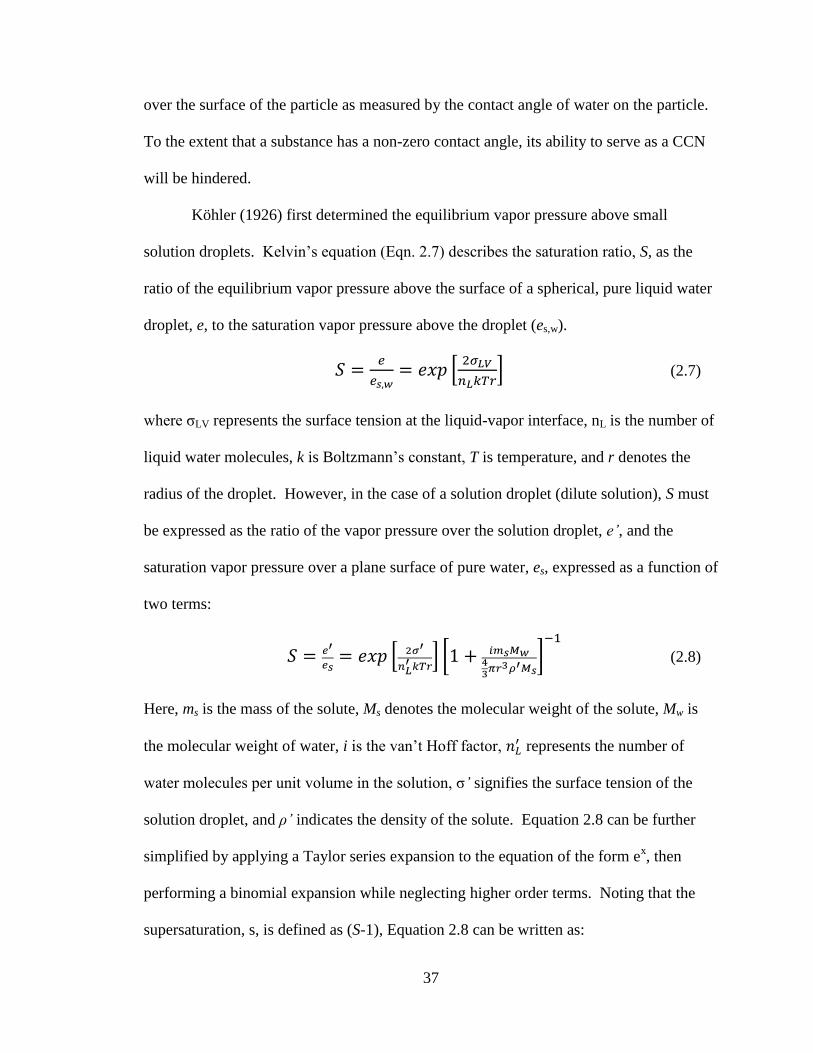
Köhler (1926) first determined the equilibrium vapor pressure above small

solution droplets. Kelvin’s equation (Eqn. 2.7) describes the saturation ratio, S, as the

ratio of the equilibrium vapor pressure above the surface of a spherical, pure liquid water

droplet, e, to the saturation vapor pressure above the droplet (es,w).

[

] (2.7)

where σLV represents the surface tension at the liquid-vapor interface, nL is the number of

liquid water molecules, k is Boltzmann’s constant, T is temperature, and r denotes the

radius of the droplet. However, in the case of a solution droplet (dilute solution), S must

be expressed as the ratio of the vapor pressure over the solution droplet, e’, and the

saturation vapor pressure over a plane surface of pure water, es, expressed as a function of

two terms:

[

] [

]

(2.8)

Here, ms is the mass of the solute, Ms denotes the molecular weight of the solute, Mw is

the molecular weight of water, i is the van’t Hoff factor, represents the number of

water molecules per unit volume in the solution, σ’ signifies the surface tension of the

solution droplet, and ρ’ indicates the density of the solute. Equation 2.8 can be further

simplified by applying a Taylor series expansion to the equation of the form ex, then

performing a binomial expansion while neglecting higher order terms. Noting that the

supersaturation, s, is defined as (S-1), Equation 2.8 can be written as:

38

(2.9)

Equations 2.8 and 2.9 represent various forms of the Köhler equation. Examples

of various K hler curves (for various aerosol species) are plotted in Figure 2.15. The

peak in a Köhler curve can be found by setting dS/dr equal to zero, and the solution

droplet radius that satisfies this condition is known as the critical radius, r*. The

corresponding supersaturation is called the critical supersaturation, sc. When the droplet

reaches its r* and sc, the droplet is said to be “activated”. The first term on the right hand

side of (2.9) is a curvature term expressive of the Kelvin effect, while the second term

signifies the solute effect. The solute term is initially important in reducing the

supersaturation required for activation, because while the droplet size is less than r*, the

relative humidity of the air adjacent to the solution droplet is less than that which is in

equilibrium with a plane surface of pure water at the same temperature. Then, if the

solution becomes more dilute, corresponding to r increasing, the associated lowering of

the equilibrium vapor pressure above its surface due to the dissolved material becomes

increasingly less. Once the droplet size surpasses that of r*, the equilibrium vapor

pressure over the small curved droplet (Kelvin curvature effect) becomes the dominant

influence. Then at some larger droplet radius, the solute term is no longer a factor and

the drop behaves as a plane surface of pure water. In other words, the addition of soluble

material to the droplet acts to depress the vapor pressure, resulting in the apparent

maximum in the equilibrium vapor pressure curve. If the ambient supersaturation

exceeds that of sc for a particular composition, the droplet formed will grow quickly to

cloud droplet size. An example of this is shown in Fig. 2.15. With an ambient

supersaturation of 0.4% and solute droplet radius of 0.1 µm, the dry particles representing

39

curves 2, 3, 4, and 6 will be able to grow droplets that reach and surpass r*, thus

activating cloud droplets (Fig. 2.15). However, the solution droplet formed via the salt

particle representing curve 5 (denoted by ‘A’) remains in stable equilibrium as a small

haze particle, as a supersaturation of 0.45% is required to activate this droplet.

The Köhler curves reveal that for a given chemical composition, as the dry

particle size increases, the critical supersaturation decreases, making it is easier to

activate larger particles. This is because for very large dry particles, the size of the

droplet at activation is very large, thus the Kelvin (curvature) effect is very small.

Therefore, if a dry particle is large enough, it can be nearly insoluble and still activate at

reasonable supersaturations. These particles, with radii typically greater than 1 µm, are

called giant CCN, or GCCN. For similar-sized dry particles, but with differing

composition, those creating the largest suppression of water vapor pressure over the

solution are generally the easiest to activate. This means that solutes which dissociate are

easier to activate than those that do not. However, this ignores the influence of the dry

particle density, as particles of the same dry size but of a different density contribute

different amounts of mass to the solution, which also must be considered. See

Pruppacher and Klett (1997), Wallace and Hobbs (1978, 2006), or Seinfeld and Pandis

(2006) for a more complete discussion of Köhler theory.

The surface tension of the solution formed by condensation onto a soluble particle

will also affect the subsequent growth of the solution droplet via the Kelvin effect (Eqn.

2.9). However, it is generally believed that surface tension effects are small (Cotton and

Yuter 2007). Another factor of importance during droplet nucleation and vapor

deposition growth is the diffusivity of vapor molecules near the surface of small droplets.

40

The vapor diffusivities are modified with a so-called accommodation coefficient in order

to account for kinetic effects. However, there is disagreement regarding the value of the

accommodation coefficient for atmospherically relevant conditions (Shaw and Lamb

1999; Laaksonen et al. 2005) even though its effect can be much stronger than many

effects associated with changes in aerosol composition (e.g. Kreidenweis et al. 2003).

2.3.3 Cloud Condensation Nuclei

The term “CCN” refers to a potential state of a particle, which is a function of the

ambient supersaturation and temperature, and cannot be conferred to a particle

independent of its environment. This is due to the fact that the solubility, wettability, and

size of a particle have important effects on its effectiveness to serve as a CCN, as

discussed in section 2.3.2 (Eqn. 2.8). For example, the initial minimum dry radius of a

particle that is activated by a supersaturation of 0.1% is 0.075 μm if the particle is

completely soluble. However, if the ratio of the soluble mass to the total mass of the

particle is only 0.2, the particle would need to have a dry radius of 0.13 μm to be

activated at the same supersaturation. At 1% supersaturation, completely wettable but

water insoluble particles need to have a radius of at least ~0.1 μm in order to serve as

CCN, whereas soluble particles can serve as CCN at the same supersaturation even if

they are as small as ~0.01 μm in radius. Most CCN consist of a mixture of soluble and

insoluble inorganic and organic components (called internally-mixed nuclei). In general,

roughly 1% of the aerosols in a continental air mass serve as CCN, while 10-20% of

aerosols serve as CCN in a maritime air mass. Typical continental (maritime) air masses

contain CCN number concentrations of about 600 (100) cm-3

at 1% supersaturation.

41

Concentrations greater than 2000 cm-3

have been observed in polluted continental air

masses. Figure 2.16 displays some observed profiles of CCN concentrations at 0.7%

supersaturation in different environments (Hoppel et al. 1973). CCN concentrations are

typically at a maximum near the surface, and values drop off with height through the

troposphere. Over land many natural CCN consist of wettable soil and dust particles.

Highly soluble salts are also produced through GPC and DPC processes and can be

dominant over land, depending on the location. Industrial processes and vegetation

burning are also significant contributors to CCN in certain regions.

2.3.4 Hygroscopicity

Hygroscopicity can generally be thought of as the measure of a solution droplet’s

capacity for growing by condensation of water vapor. The solute term in Equations 2.8

and 2.9 is a rough measure of a particle’s hygroscopicity and is equal to the mole fraction

of water (xw). From Raoult’s law, the mole fraction of water is analogous to the water

activity, aw, meaning that the solute term expresses the water activity, which is a measure

of the hygroscopicity. A non-idealized expression for xw is given in Equation 2.10:

[

( )

]

(2.10)

where ns and nw denote the number of solute and water molecules, respectively. The

various Köhler curves plotted in Fig. 2.15 indicate that hygroscopicity has a significant

influence on sc.

Another way to express the saturation ratio over an aqueous solution droplet is

given by:

42

(

) (2.11)

where σs/a is the surface tension of the solution/air interface, R is the universal gas

constant, and D is the diameter of the droplet. Recently, Petters and Kreidenweis (2007)

introduced functional representation of hygroscopicity. Making use of (2.10) and (2.11),

the expression for aw can be simplified to a function of the ratio between the dry particle

volume (Vs) and water volume (Vw) using a single parameter, κ, that is defined through its

effect on the water activity of the solution. This concept is expressed mathematically as:

(2.12)

The κ parameter can therefore be represented as:

(2.13)

The κ parameter accounts for not only the water activity but also the nature of the solute,

dissociation, and nonidealities of the solution formed. Furthermore, the hygroscopicity of

particles containing more than one chemical species, known as internal mixtures, can be

computed simply as a volume‐weighted average κ:

∑ (2.14)

where εi is the volume fraction of each component (i) of the solute and κi is the κ

parameter for constituent i. This expression assumes no interaction between the different

solute ions in the solution.

Values of κ for various aerosol constituents have been determined experimentally

(e.g., Petters and Kreidenweis 2007), most varying between 0 and 1.2 (Table 2.3). Figure

2.17a shows various values of κ for a range of supersaturations and particle dry diameter,

while Fig. 2.17b displays plots of various Köhler curves, representing the equilibrium

43

vapor pressure for solution droplets of the same radius but of varying values of κ. Since

its introduction, κ has been used to represent hygroscopicity in both observational (e.g.

Gunthe et al. 2009; Koehler et al. 2009) and modeling studies (e.g., Reutter et al. 2009;

Eidhammer et al. 2009; Ward and Cotton 2011).

2.3.5 Ice Nucleation

Homogeneous nucleation of ice particles refers to two mechanisms: sublimation

and the freezing of cloud droplets. In the case of sublimation, small ice crystals form via

the chance aggregation of vapor molecules. However, this process requires very high

supersaturations with respect to ice and such low temperatures (< -60°C) that it does not

take place in the troposphere. For the homogeneous freezing of a cloud droplet to occur,

enough ice-like water molecules must come together within the droplet to form an ice

embryo that is large enough to survive and grow, associated with the chance aggregation

of liquid molecules. If an ice embryo within a droplet exceeds a certain critical size, its

growth will produce a decrease in the energy of the system. Homogeneous nucleation

occurs at roughly –41°C for droplets approximately 1 μm in diameter, and at about –35°C

for drops 100 μm in diameter.

Nucleation via the assistance of an aerosol particle is a process known as

heterogeneous nucleation. Since the formation of an ice structure is aided by a freezing

nucleus (called ice nuclei, or IN), and the ice embryo also starts off with the dimensions

of the freezing nucleus, heterogeneous nucleation can occur at much higher temperatures

compared to the homogeneous nucleation of freezing and at lower supersaturations

compared to the formation of ice by homogeneous nucleation via sublimation. IN have

44

one of four basic modes of action: vapor deposition, condensation-freezing, immersion-

freezing, and contact-freezing. Vapor deposition nucleation refers to the direct transfer of

water vapor to a nucleus resulting in the formation of an ice crystal, which requires

supersaturations with respect to ice and low temperatures. Condensation-freezing, or

sorption, refers to the condensation of water vapor on a nucleus to form an embryonic

droplet, which is then followed by freezing. This process requires the air to be

supersaturated with respect to water. However, if this is the case, a suitable particle may

serve either as a condensation-freezing nucleus or as a deposition nucleus. In practice, it

is not easy to distinguish between the deposition and condensation-freezing modes.

However, the surface tension at the liquid-surface interface for immersion freezing is

roughly four to six times smaller than the surface tension at the vapor-surface interface

for vapor deposition. As a consequence, substances more “easily” serve as freezing

nuclei compared to deposition nuclei (e.g., Fletcher 1958; Young 1993).

Immersion-freezing refers to the nucleation of a cloud droplet or raindrop by an

ice nucleus that is immersed within the drop. In this process, water molecules in the

droplet collect onto the surface of the particle to form an ice-like structure that may

increase in size and cause the droplet to freeze. The most accepted theory of immersion-

freezing is singular theory (Marcolli et al. 2007; Vali 2008), which holds that at a given

degree of supercooling, the likelihood that a drop of a given size will freeze depends

solely on the likelihood that the drop contains an active freezing nucleus, a process that is

independent of time to only a minor degree (Vali and Stanbury 1966). The stochastic

theory of immersion-freezing (e.g., Bigg 1953; Dufour and Defay 1963) is less accepted

however there is still some active debate on this.

45

Contact nucleation refers to the freezing of a supercooled drop by a nucleus that

makes contact with the surface of the drop while the drop is in a supercooled state. In the

atmosphere, contact nucleation can produce considerable time-dependence in the

nucleation process, because it depends both on the probability that an aerosol particle

makes contact with a supercooled drop and the probability that the aerosol particle acts as

an active freezing nucleus. Laboratory experiments suggest that some particles can cause

a drop to freeze by contact freezing at temperatures several degrees higher than if they

were embedded in the drop (Fletcher 1962; Levkov 1971; Gokhale and Spengler 1972;

Pitter and Pruppacher 1973). Laboratory experiments by Durant and Shaw (2005)

showed that as droplets evaporate, embedded aerosol particles become increasingly likely

to penetrate the air-water interface layer and promote freezing, suggesting that contact

freezing may be just as effective from the inside-out as from the outside-in.

2.3.6 Ice Nuclei

In general, particles with the ability to nucleate ice without specifying a mode of

action are called IN. However, one should note that the temperature at which a particle

can cause ice to form generally depends upon the mechanism by which the particle

nucleates the ice as well as upon the previous history of the particle. The basic

distinction that must be made is whether nucleation occurs from the vapor or liquid phase

(Vali 1985). The activity of a particle as a condensation-freezing or a deposition nucleus

depends not only on the temperature but also on the supersaturation of the ambient air.

The effect of supersaturation on measurements of IN concentrations is shown in Figure

46

2.18, where it can be seen that at a constant temperature the greater the supersaturation

with respect to ice the more particles serve as IN.

Aerosol particles with molecular spacing and crystallographic arrangements

similar to those of ice (which has a hexagonal structure) tend to be effective as IN,

although this is neither a necessary nor a sufficient condition for a good ice nucleus.

Almost all particles that may serve as IN are virtually insoluble in water, as soluble

particles disintegrate under the action of water, and hence, the molecular structural

requirement for ice nucleation cannot be maintained. Furthermore, the radius of the

particle must have a size comparable to or larger than that of a critical ice embryo

(Georgii and Kleinjung 1967; Berezinski et al. 1986). Therefore, an effective particle

must generally be greater than 0.1 µm. Lastly, laboratory studies indicate that ice

nucleation is preferred on those substrates that have pits and steps on their surfaces.

The identification of the chemical composition of particles found at the center of

ice crystals has provided much information regarding the likely origins of IN. The major

source of IN is the earth’s surface, primarily arid regions such as deserts and dry lake

beds. This is because some inorganic soil particles, mainly clays, can nucleate ice at

fairly high temperatures (i.e., above –15°C), and they likely play an important role in

nucleating ice in clouds. Desert dust is known to be very effective IN (DeMott et al.

2003). In a study by Kumai (1961), 87% of the snow crystals collected on the ground

had clay mineral particles at their centers, of which more than half of them were

kaolinite. Of course merely the presence of dust particles does not prove that they served

as IN. Secondary sources of IN include volcanoes and combustion processes that create

inorganic IN. Other sources of IN include metal oxides produced by industrial processes,

47

organics produced by vegetation burning, certain strains of bacteria (Bigg and Turton

1988; Bigg 1988, 1990; Vali et al. 1976; Yankofsky et al. 1981; Levin and Yankofsky

1983; Levin et al. 1987), other organics such as decayed plant matter (Schnell and Vali

1976), aerosols found in seawater rich in plankton, and pollen (Von Blohn et al. 2005).

In some cases, after a particle has served as an ice nucleus, and all of the visible

ice has been evaporated from it, but the particle has not been warmed above 0°C or

exposed to a relative humidity with respect to ice below 50%, the particle may

subsequently serve as an ice nucleus at a temperature a few degrees higher than it did

initially (Roberts and Hallett 1968). This process is called preactivation.

Shown in Figure 2.19 are plots of IN concentrations as a function of temperature

for a variety of locations. These observations suggest that there is no systematic variation

in IN concentration with geographic location, at least over extended periods of time when

neglecting short-term variations. In addition, few studies have found a relationship

between total aerosol concentration and IN concentration. However, some studies have

suggested a correlation between IN concentrations and those of the large mode of the

total aerosol size distribution (Georgii and Kleinjung 1967; Berenzinsky et al. 1986;

DeMott et al. 1994). For a typical continental air mass at –20ºC, IN concentrations are

around 1 L-1

, which given the total aerosol population suggests that only one in 106

aerosols serve as IN (Fletcher 1962). Many parameterizations assume IN concentrations

to drop off with height (e.g., DeMott et al. 1994). However, this is not always the case.

Figure 2.20a illustrates measurements of IN concentrations with height taken over the

Arctic ice sheet during the 1998 FIRE/SHEBA field campaign. Maximum concentrations

(near 20 L-1

) are found above the boundary layer capping inversion. Figs. 2.20b-d

48

display various profiles of IN associated with enhanced dust concentrations within the

Saharan Air Layer (SAL) observed during the Cirrus Regional Study of tropical Anvils

and Cirrus Layers-Florida Area Cirrus Experiment (CRYSTAL-FACE) field campaign

(DeMott et al. 2009).

2.3.7 Ice Multiplication

Ice crystal concentrations in actual clouds are often not represented by the

concentrations of IN measured or expected to be activated in such environments. In

particular, it has been found that at temperatures warmer than –10°C, the concentration of

ice crystals can exceed the concentration of IN activated at cloud top temperature by

three to four orders of magnitude (Braham 1964; Koenig 1963; Mossop 1970; Mossop

and Ono 1969; Mossop et al. 1967, 1968, 1972; Magono and Lee 1973; Auer et al. 1969;

Hobbs 1969, 1974). The effect is greatest in clouds with broad drop-size distributions

(Koenig 1963; Mossop et al. 1968, 1972; Hobbs 1974). Multiple hypotheses have been

proposed to account for such high ice particle concentrations, including drop

fragmentation, ice crystal fracturing, ice crystal rime splintering, spuriously high

supersaturation production, and ice particle evaporation (Pruppacher and Klett 1997).

Many of these theories have been shown to be unlikely significant contributors to ice

crystal concentrations. The concept of secondary ice particle production during the

riming growth of ice particles, also known as the Hallett-Mossop or rime-splinter process,

has been given the most attention and quantified in models. Laboratory studies by Hallett

and Mossop (1974) and Mossop and Hallett (1974) indicated that copious amounts of

splinters are produced during ice particle riming, but only under selective conditions.

49

The temperature must be in the range of –3ºC to –8ºC, a substantial concentration of large

cloud droplets with radii greater than 12 µm must be present, and these large droplets

must be coexisting with smaller cloud droplets, possessing radii smaller than roughly 6

µm. When these conditions were met, an optimum average splinter production rate of

one secondary ice particle for 250 large droplet collisions occurred near –5°C. This

process is consistent with field observations, where the greatest departure from IN

estimates of ice crystals occurs when clouds contain graupel particles and frozen

raindrops (Hobbs and Cooper 1987). However, other observations suggest that the

generation of secondary particles during the evaporation of ice particles may also

considerably add to ice multiplication (Hobbs and Rangno 1985, 1990; Oraltay and

Hallett 1989; Dong et al. 1994; Rangno and Hobbs 1994; Cooper 1995; Field et al. 2001;

Cotton and Field 2002).

2.4 Precipitation formation

2.4.1 Raindrop Growth Mechanisms

Collision-coalescence involves the initial formation of a few large cloud drops,

followed by their rapid and substantial growth as they fall through the air and collide with

smaller cloud droplets, coalescing to form larger drops. This process can operate in

clouds containing cloud droplets, whether they are situated above or below the 0ºC level.

A drop will not collect all of the cloud droplets lying in its path due to the flow of air

around the falling drop. Calculated values of the collision efficiency, defined as the ratio

of the cross-sectional area over which droplets are collected to the geometric cross-

sectional area of the collector drop, indicate that the collision efficiency is negligible until

50

a collector drop obtains a radius of ~20 μm. Once this size, the droplet grows

increasingly fast by collision. Moreover, as droplets get larger, their cross sectional areas

and fall velocities increase, thereby increasing the collection kernel between large and

small drops. Hence a few droplets need to grow to a radius of 20 μm by condensation if a

cloud is to form raindrops by collision and coalescence. However, the initial broadening

of the drop size distribution (DSD) leading to the production of drops this large is not

fully understood. Four mechanisms have been proposed to explain how these larger

droplets can form. They are the role of giant cloud condensation nuclei (GCCN),

turbulence influences on condensation growth, turbulence influences on droplet collision

and coalescence, and radiative cooling of drops to form precipitation embryos.

Multiple observations (e.g., Woodcock 1953; Nelson and Gokhale 1968;

Hindman 1975; Johnson 1976, 1982; Hobbs et al. 1980) have shown the presence of

potentially significant concentrations of aerosol particles with sizes as large as 100 μm.

Approximately only one in 105

or 106

CCN are giant particles (Woodcock 1953).

Nevertheless, they can have a significant impact on the development of precipitation by

serving as coalescence embryos (Johnson 1982; Feingold et al. 1999; Yin et al. 2000).

The droplets that nucleate onto these particles are large enough for coalescence to start

immediately, even before the droplet reaches its critical size, based on the Köhler

equation. Early observations suggest that this can occur if the nuclei are completely

soluble, very large and wettable, or are mixed particles with a soluble coating (e.g., Levin

et al. 1996).

Convective clouds are composed of a series of updrafts of varying intensities.

The least vigorous updrafts at cloud base produce the lowest droplet concentration during

51

CCN activation. Turbulence further contributes to the entrainment of dry environmental

air, reducing the liquid water content (LWC) below the adiabatic value and diluting the

droplet concentration below its initial value after CCN activation. Turbulence also

contributes to the continuous mixing of convective cells, smoothing out their differences

in terms of concentration and droplet growth. Turbulence can also influence the collision

and coalescence process by enhancing collision efficiencies, because droplets are able to

cross streamlines more efficiently in turbulent flow compared to laminar flow. Larger

droplets, having more inertia, will be affected more by turbulence than smaller drops.

This effect is minimal for droplets smaller than 20μm in diameter (Koziol and Leighton

1996). Turbulence can also cause fluctuations on vertical fall velocities and horizontal

motions, such that the collection kernel is enhanced relative to that defined in laminar

flow (Pinsky and Khain 1997; Khain and Pinsky 1997).

Regarding radiative effects, consider a population of droplets residing near cloud

top for a sufficient amount of time. The droplets will emit radiation to space quite

effectively in a relatively dry and cloud free atmosphere aloft. The droplets will thus be

cooler than if radiative effects were not considered. The saturation vapor pressure at the

surface of the droplets will therefore be lowered and the droplets will grow faster.

However, as radiative cooling is proportional to the cross sectional area of a droplet, its

effect is much greater on larger droplets than small ones (Roach 1976; Barkstrom 1978;

Guzzi and Rizzi 1980; Austin et al. 1995; Harrington et al. 1997). This process is

inefficient in cumulus clouds due to their vigorous overturning.

Once precipitation embryos form they rapidly collect smaller droplets. They then

transform into drizzle and raindrops in a matter of minutes if the liquid water content in

52

clouds is great enough. The final size spectrum of the raindrops is determined by the

liquid water content in the clouds, as well as their trajectories through updrafts and

downdrafts in the cloud.

Raindrops can also form as a result of “cold rain” processes in mixed phase

clouds, that is, rain formed due to the melting of ice crystals, graupel, and/or hail.

Regardless of the raindrop formation process, the drop breakup process impacts the

resulting DSD. Raindrops may breakup either spontaneously or by colliding with other

raindrops.

2.4.2 Ice Particle Growth Mechanisms

In clouds lower than 0°C containing relative humidity greater than 100% with

respect to ice, ice crystals may grow by vapor deposition (Pruppacher and Klett 1997). In

regions of clouds lower than 0°C, supercooled water droplets can be present with or

without the presence of coexisting ice particles. In a mixed-phase cloud dominated by

supercooled droplets the supersaturations with respect to ice are much greater than the

supersaturations of cloudy air with respect to water. Consequently, ice particles will

grow from the vapor phase much more rapidly and at the expense of liquid droplets

(Wegener 1911; Bergeron 1933; Findeisen 1938). This can lead to a variety of ice crystal

types, some of which may be large enough to precipitate. Ice particles in a cloud may

collide and aggregate with each other, leading to larger particles, which are called

aggregates. On the other hand, modeling studies have shown that the rapidity of

glaciation is greater in the presence of supercooled raindrops (Cotton 1972; Koenig and

Murray 1976; Scott and Hobbs 1977), because supercooled raindrops (and drizzle-sized

53

drops) may freeze by collection of ice crystals. As such, the rapidity of glaciation in

mixed-phase clouds increases (nonlinearly) with increasing liquid water contents.

Ice particles can also grow in mixed-phase clouds by colliding with and collecting

supercooled cloud droplets that proceed to instantaneously freeze onto them, a process

known as riming. If the degree of riming is such that the ice particle has grown to a point

where the habit of the original ice particle is no longer discernible, the ice particle is

called graupel. In deep cumulonimbi where updrafts and LWCs are high enough, graupel

particles, frozen raindrops, and large aggregates can serve as embryos for hailstone

formation (Heymsfield et al. 1980). At first the density of graupel particles is relatively

low, because the collected frozen droplets are loosely compacted on the surface of the

graupel particle. As the ice particle grows, it falls faster, sweeps out a larger cross-

sectional area, and its growth by collection of supercooled droplets increases

proportionally. As the growth rate increases, the collected droplets may not freeze

instantaneously on impact, and the unfrozen water can flow over the surface of the

hailstone, filling in the gaps between collected droplets. The density of the ice particle

approaches that of pure ice and is classified as a hailstone. The ultimate size of the

hailstone is dependent upon the amount of supercooled liquid water in the cloud and the

time that the growing hailstone can remain in the high rainwater region. The time that a

hailstone can remain in the high liquid water content region, in turn, is dependent on the

updraft speed and the fall velocity of the hailstone itself. The optimal situation for hail

growth is therefore when the ice particle fall speed nearly matches the updraft speed

(Foote 1984), as the hailstone will slowly ascend or descend while it collects cloud

droplets at a very high rate. Eventually the hailstone fall speed will exceed the updraft

54

speed or move into a region of weak updraft or downdraft and begin to fall. The size of

the hailstone upon reaching the surface will decrease the longer it falls through air greater

than 0°C. Therefore, hail growth is most likely if the convective storm updrafts are

strong, the liquid water contents are large, the storm is deep and long-lived, and the

melting level is low relative to the ground (Foote 1984).

2.5 Mineral Dust Characteristics

Dust observations from the southwestern U.S. are rather limited. Haywood et al.

(2003), utilizing observations from the Saharan Dust Experiment (SHADE), found that

maximum dust number concentrations within dust plumes lofted from the Saharan Desert

often exist near the marine boundary layer (~1800 m AGL) or in an elevated region

above 3 km, with concentrations varying anywhere between 500 and 2000 cm-3

. With

such high concentrations observed in specific regions of the world, many have argued

that mineral dust may have substantial impacts on clouds and precipitation on a variety of

time and spatial scales via direct radiative and indirect microphysical effects.

Aerosols impact radiation balance both directly through the absorption, scattering,

and emission of solar radiation and indirectly by modifying cloud properties that are

associated with cloud radiative feedbacks. Due to the radiative properties of mineral

dust, a suspended layer of dust enhances the absorption of solar radiation within that

layer. This results in higher temperatures and thus increased atmospheric stability within

that layer (e.g., Brooks 2000; Haywood et al. 2003; Fan et al. 2004). Results from

numerical simulations of high shear/high CAPE environments performed by Ziegler et al.

(2010) suggested that inversions tend to support the development of isolated, long-lived

55

supercells, while more horizontally-homogeneous, inversion lacking regions allow for the

development of secondary convection followed by rapid upscale growth, thus instead

favoring long-lived mesoscale convective systems as opposed to supercell storms.

Stokowski (2005) performed numerical model simulations to investigate direct radiative

impacts of mineral dust based on SHADE data. In all simulated layers where mineral

dust was present, the radiation streams (both longwave and shortwave) were reduced in

intensity to some degree, due to the strongly absorbing nature of the mineral dust. These

results were consistent with results seen in SHADE (Haywood et al. 2003). The main

effect was seen through the temperature field, as dramatic heating occurred within the

concentrated dust layers. The impact of the presence of a significant dust layer resulted

in increasing the associated temperature at a rate of 2-3°C per day. Dunion and Velden

(2004) found evidence that the SAL might suppress tropical cyclone activity in the

Atlantic via this process, i.e., the added heating due to the presence of dust locally

enhancing atmospheric stability.

Few datasets exist that contain direct measurements of the hygroscopicity and

CCN activity of natural, heterogeneous mineral dust particles. Some studies have

presented evidence that small dust particles may serve as CCN once coated with soluble

material (Levin et al. 1996; Fan et al. 2004). Laboratory studies which measured the

heterogeneous reactions of gaseous phase SO2 and NOx with mineral dust found that

modestly soluble species were formed on the surface of the particles (Laskin et al. 2005;

Usher et al. 2003). Dust particles may also become mixed nuclei through collisions and

coagulation with soluble particles in the atmosphere or by mixed aerosol preactivation

(Twohy and Poellot 2005). Pollution and secondary organic aerosol precursor gases may

56

form low volatility products that can deposit on the surface of dust. Kelly et al. (2007)

found that accounting for very small mass fractions of even modestly soluble species can

increase the modeled ability of a particle to serve as a CCN. As such, submicron dust

particles, composed primarily of insoluble minerals, are typically modeled as CCN

inactive until they have become mixed with hygroscopic material such as various sulfates

or nitrates (e.g., Fan et al. 2004; Liu et al. 2005; Twohy et al. 2009). Koehler et al.

(2009) tested the CCN activity of various dust species in the submicron range, including

Arizona Test dust, thought to be representative of dust with very low soluble material

content in the southwestern U.S. The dry-generated particles served as CCN at lower

supersaturations than predicted for purely insoluble, wettable particles. Dust particles

that were suspended in water prior to reaerosolization (wet-generation) were significantly

more hygroscopic than the dry-generated particles, but both methods produced particles

which were more CCN active than predicted for insoluble, wettable particles and their

activity indicated that sub-400 nm diameter particles of Arizona Test dust should readily

serve as CCN at typical cloud supersaturations (0.2-0.3%).

As discussed in section 2.3.2, the solubility requirement for aerosols serving as

CCN decreases with increasing particle size as the curvature term in the Köhler equation

becomes the dominant factor. Many suspended dust particles are greater than 1 µm in

radius, and studies suggest that these large particles can effectively serve as GCCN (e.g.,

Levin et al. 1996; Levin et al. 2005; Seinfeld and Pandis 1998; Koehler et al. 2009).

It has long been suggested through laboratory measurements and observations that

mineral dust aerosol may potentially serve as IN and heterogeneously nucleate the ice

phase in the atmosphere (Schaefer 1949; Isono et al. 1959; Gagin 1965; Zuberi et al.

57

2002; Demott et al. 2003; Sassen et al. 2003). Roberts and Hallett (1968) examined the

ice nucleation ability of kaolinite, montmorillonite, gypsum, calcite, vaterite, albite, and

biotite particles with diameters between 0.5 and 3 μm. The warmest temperature at

which one in 104

particles could initiate the ice phase varied between –10.5 and –26°C.

Preactivation caused them to freeze more easily, with threshold temperatures ranging

from –4 to –12°C. Schaller and Fukuta (1979) found similar results for kaolinite.

Archuleta et al. (2005), using a continuous flow diffusion chamber (CFDC, Rogers

1988), examined the heterogeneous freezing of mineral dust surrogates and found a clear

size dependence in the required onset relative humidity with respect to ice (RHi) for ice

nucleation at a fixed temperature, with the largest particles (~0.2 μm) nucleating ice at

RHi as low as ~135% and smaller particles requiring higher RHi. Similar studies found

that supersaturations with respect to ice of just several percent were sufficient to nucleate

ice crystals using Arizona Test dust with a median diameter of ~0.5μm (Mangold et al.

2005). Salam et al. (2006) found that montmorillonite and kaolinite nucleated ice

between 110-115% and 115-125% RHi, respectively. In addition, montmorillonite

(kaolinite) required temperatures of –15°C (–22°C), and the fraction of particles

nucleated increased with decreasing temperature at water saturated conditions.

DeMott et al. (2003) determined the composition of residual ice nuclei particles

that were measured in a CFDC from free troposphere air sampled in Colorado and found

that while mineral dust particles comprised only ~1% of the total submicron particles,

they represented 33% of the heterogeneously nucleated ice crystals, 25% of which

contained measurable sulfate or organic coatings. However, none of the samples

supported ice formation at temperatures warmer than around –30°C. Studies suggest that

58

the particles which initiate the ice phase at the lowest supersaturations are those with the

smallest contents of soluble material (Zuberi et al. 2002; Hung et al. 2003).

Koehler et al. (2009) tested the IN activity of various dust species, including

Arizona Test dust, finding that at temperatures below –40°C, dry- and wet-generated

particles appeared to serve as deposition IN, however, much lower ice supersaturations

were required for the dry-generated particles. As the temperature increased, the particles

produced by both generation methods required water saturation conditions before

initiating freezing, indicating a shift from deposition to condensation freezing at

temperatures warmer than –40°C. Larger particles were able to serve as condensation IN

at warmer temperatures than observed for smaller particles. Ice formation behavior of the

dry-generated dust showed little dependence on temperature between –60 and –40°C,

nucleating ice on 1% of particles at a similar RHi for any temperature, but with a strong

dependence on particle size and sample type.

The data suggest that atmospheric dust particles may impact warm and cold cloud

formation via direct radiative and indirect microphysical effects. Even the limited CCN

activity determined for some samples could be relevant to cloud drop formation in the

atmosphere, as dust plumes generally contain relatively large number concentrations of

particles with diameters larger than 400 nm. Therefore, the potential for dust particles to

serve as large and giant CCN must be considered in determining the role of dust in

precipitation processes. Even small number concentrations of heterogeneous IN and

GCCN can strongly impact cloud processes (e.g., Johnson 1982; Feingold et al. 1999;

Yin et al. 2000; Saleeby and Cotton 2005). However, with the potential to serve as CCN,

59

GCCN, and IN, disagreement exists over how mineral dust indirectly affects clouds and

precipitation (e.g., Levin et al. 1996; Rosenfeld et al. 2001; Levin et al. 2005).

2.6 Aerosol effects on clouds and precipitation

Aerosols, both natural and anthropogenic, may impact clouds and precipitation on

a variety of scales. There has been growing evidence that dust from arid regions around

the world, particularly from the Sahel and Asian desert regions, can influence the

microphysics of warm and cold cloud formation (DeMott et al. 2003b; Mahowald and

Kiehl 2003; Sassen 2002). The concentrations of CCN, GCCN, and IN in the atmosphere

will alter the concentrations and size distributions of hydrometeors and thus the radiative

properties of the cloud. Given the same liquid water content (LWC), increasing CCN

concentrations results in a greater number of cloud droplets that are of smaller sizes than

would have otherwise formed with fewer CCN. This results in narrower cloud droplet

spectra and reduced collision efficiencies, making the cloud more colloidally stable and

less efficient at producing warm rain. Thus, increasing CCN concentrations tends to

reduce the warm rain process (Gunn and Phillips 1957; Squires 1958; Kaufman and

Nakajima 1993; Borys et al. 1998; Rosenfeld 1999, 2000). Albrecht (1989) and Jiang et

al. (2002) found that increased CCN led to a suppression of drizzle in marine

stratocumulus clouds. However, dynamical feedbacks of drizzle suppression are complex

and not well understood. Two-dimensional simulations of stratocumulus clouds by

Feingold et al. (1996) showed that the evaporation of drizzle just below cloud base acts to

destabilize the boundary layer, promoting convection below cloud base and leading to

60

enhanced cloud albedo. Conversely, the boundary layer may become more stable if the

drizzle reaches the surface (Stevens et al. 1998; Jiang et al. 2002).

The role of GCCN adds complexity to how aerosols may impact the warm rain

process, as studies have shown that greater concentrations of GCCN actually broaden the

initial cloud droplet spectra by creating larger cloud droplets. This enhances collision

and coalescence processes, and therefore tends to increase precipitation (Feingold et al.

1999; Hobbs et al. 1970; Eagan et al. 1974; Braham et al. 1981; Rosenfeld et al. 2002).

This effect is most often observed in high CCN environments (Feingold et al. 1999).

Levin et al. (1996) found that dust particles coated with sulfate acted as GCCN,

accelerating the precipitation process. Rosenfeld et al. (2001) and Mahowald and Kiehl

(2003) found for the same region (Eastern Mediterranean) that dust decreased the

precipitation efficiency by enhancing CCN concentrations and suppressing droplet

coalescence. However, the decrease in precipitation efficiency observed by Rosenfeld et

al. (2001) was in comparison to conditions of relatively clean maritime clouds, whereas

Levin et al. (1996) compared to already polluted clouds containing high concentration of

sulfate aerosol from Europe, thus finding that dust enhanced precipitation efficiency.

In deep convective clouds, the rapidity of glaciation is dependent upon the

presence of drizzle drops and large supercooled raindrops (Cotton 1972; Koenig and

Murray 1976; Scott and Hobbs 1977). When CCN concentrations are high, liquid-phase

precipitation collection processes are suppressed and supercooled raindrops are few in

number. Small ice crystals must then grow to several hundred microns in diameter

before they begin collecting cloud droplets. This suppresses the riming process in air

61

masses with high CCN concentrations (Borys et al. 2000, 2003) and thus secondary ice

particle production by the rime-splintering process.

Multiple simulations of deep convective clouds have demonstrated that enhancing

CCN concentrations produces an initial suppression in precipitation formation, resulting

in more supercooled water aloft, creating stronger updrafts and more vigorous convection

aloft via enhanced latent heating effects from freezing (Khain et al. 2004; Lynn et al.

2005; Seifert and Beheng 2006; van den Heever et al. 2006 ). This may result in an

increase in precipitation rate in polluted systems. However, due to feedbacks onto other

dynamics such as secondary convection, a decrease in total precipitation can still occur

(Lynn et al. 2005; van den Heever et al. 2006). In particular, van den Heever et al.

(2006) evaluated possible indirect microphysical effects of dust on Florida

thunderstorms, utilizing observations from the CRYSTAL-FACE field campaign to

initiate the simulations. The added particulates acted as enhanced concentrations of

CCN, GCCN, and IN in various simulations. As mentioned, increased CCN

concentrations suppressed warm rain processes but resulted in stronger updraft via latent

heating. In simulations where GCCN and IN concentrations were increased by dust,

enhanced glaciation resulted, which led to further dynamical invigoration of the

convective updrafts as well as enhanced precipitation (Simpson et al. 1967; Rosenfeld

and Woodley 1989, 1993). The CCN effect was a dominant influence initially. Once a

large amount of cloud water was transported vertically, the GCCN impact became more

important during the mature and dissipating phases of the convection, as glaciation is

more effective in ice phase interactions. For example, larger droplets are more

effectively collected by ice particles, and larger droplets undergo homogeneous freezing

62

more rapidly. Greater concentrations of GCCN yield greater amounts of larger droplets,

and hence the associated release of latent heat upon interacting with ice is greater.

Stephens et al. (2004) and Teller and Levin (2006) also found an increased occurrence of

deep convection when dust was added to their two-dimensional model simulations.

However, Teller and Levin (2006) found that GCCN enhancement decreased

precipitation in clean clouds (CCN concentrations less than 600 cm-3

) but increased the

total precipitation for polluted clouds, and that increasing IN concentrations reduced total

precipitation in all but the most polluted cases. The reduced precipitation efficiency due

to increasing IN concentrations resulted in the transport of water vapor from lower levels

to the mid troposphere. The enhancement in precipitation from increased GCCN

concentrations was found to be due to increased graupel production within the clouds,

while the IN decreased the graupel content within the modeled clouds by creating small

pristine ice crystals. Rosenfeld et al. (2002) noted that precipitation in polluted clouds

could be initiated more easily in the presence of GCCN, but did not comment on the

amount of precipitation produced compared to a cleaner cloud. IN concentrations have

also been shown to be critical to the initial formation of hail (Danielson 1977). As a

possible example, soil dust particles originating from the Texas panhandle have been

found at the centers of hailstones from convective storms in the Southern Plains (Gitlin

1978).

Not many studies have addressed potential aerosol impacts on supercell

thunderstorms. However, van den Heever and Cotton (2004) addressed possible

microphysical effects utilizing three-dimensional idealized model simulations with single

moment microphysics. They found that simulations favoring larger hail diameters

63

reduced the total surface area of the hailstone population, which resulted in reduced

evaporative cooling and melting rates compared to the simulations with smaller

hailstones. The reduced evaporative cooling yielded weaker low-level downdrafts and

weaker, shallower cold-pools at the surface. Simulations by Gilmore et al. (2004) found

similar results with respect to rain DSDs. Snook and Xue (2008) extended the work of

van den Heever and Cotton (2004) and Gilmore et al. (2004) to tornadogenesis, verifying

that larger raindrops and hailstones yielded warmer cold-pools via reduced evaporative

cooling. In addition, the larger hydrometeors, with greater terminal fall speeds, were not

advected as far from the main updraft before falling to the ground, reducing the areal

coverage of precipitation. This positioned the gust front closer to the storm center,

permitting vertically-oriented updrafts and vertical alignment of low- and mid-level

vertical vorticity. This in turn increased the dynamic suction effect by the mesocyclone

(Rotunno and Klemp 1982) and associated low-level vertical stretching, thereby

increasing the potential for tornadogenesis in the simulations favoring larger

hydrometeors. Simulations by Storer et al. (2010) found that enhancing CCN

concentrations in deep convection led to a reduction in the warm rain process but larger

raindrops compared to the simulations with fewer CCN. As a result, total precipitation

was reduced, as was net evaporative cooling within downdraft regions. This produced

weaker, shallower cold-pools.

The radiative properties of mineral dust together with the potential for mineral

dust to serve as CCN, GCCN, and IN suggest that mineral dust may potentially impact

the development of supercell storms, including influencing the pre-storm environment,

64

microphysical evolution such as hailstone size, resulting cold-pool characteristics, and

even tornadogenesis.

It should be noted that orographic clouds, both warm-based and mixed-phase, are

particularly susceptible to aerosol effects (Levin and Cotton 2009). In addition, dust may

impact clouds via indirect radiative effects (Twomey 1974, 1977; Hansen et al. 1997;

Rosenfeld et al. 2001; Chylek et al. 2006). However, this study does not address

potential dust impacts on orographic clouds or dust indirect radiative effects on clouds.

65

Table 2.1: The original Fujita scale with wind speed thresholds and damage descriptions

(adapted from Fujita 1971).

Rating Scale

Wind Speed (mph)

Wind Speed (ms-1)

Damage Description

F0 40-72 18-32 Light damage: Some damage to chimneys F1

73-112

33-50

Moderate damage: Peel surfaces off roofs; mobile homes pushed off foundations or overturned

F2

113-157

51-70

Considerable damage: Roofs torn off of framed houses; mobile homes destroyed

F3

158-206

71-92

Severe damage: Roofs and some walls torn from well-constructed houses

F4

207-260

93-116

Devastating damage: Well-constructed houses leveled; structure with weak foundations blown off some distance

F5

261-318

117-142

Incredible damage: Strong frame houses lifted from foundation and carried great distances to disintegrate

66

Table 2.2: The enhanced Fujita scale with wind speed thresholds (adapted from Marshall

et al. 2004).

Rating Wind Speed (mph) Wind Speed (ms-1)

EF0 65-85 29-38 EF1 86-109 39-49 EF2 110-137 50-61 EF3 138-167 62-75 EF4 168-199 76-89 EF5 ≥ 200 ≥ 90

67

Table 2.3: Mean values of CCN-derived κ for various aerosol constituents. PK07 denotes

values taken from Petters and Kreidenweis (2007; their Table 1).

Compound CCN-derived κ Source

(NH4)SO4 0.61 PK07

NH4NO3 0.67 PK07

NaCl 1.28 PK07

H2SO4 0.71 Shantz et al. (2008)

NaNO3 0.88 PK07

NaHSO4 0.91 PK07

Na2SO4 0.8 PK07

(NH4)3H(SO4)2 0.65 PK07

malonic acid 0.227 PK07

glutaric acid 0.088 PK07

glutamic acid 0.182 PK07

succinic acid 0.231 PK07

adipic acid 0.096 PK07

levoglucosan 0.208 PK07

phthalic acid 0.051 PK07

homophthalic acid 0.094 PK07

leucine 0.002 PK07

pinic acid 0.248 PK07

pinonic acid 0.106 PK07

norpinic acid 0.182 PK07

poly(acrylic) acid 0.051 PK07

Suwanee River fulvic acid 0.067 PK07

α-pinene 0.1 PK07

β-pinene 0.1 PK07 dry-generated Arizona Test Dust 0.025 Koehler et al. (2009) Dry-generated mineral dust with low

hygroscopicity content by mass and an

insoluble core

0.03 Koehler et al. (2009)

68

Figure 2.1: Mean hodograph for 62 tornado outbreak cases. The soundings are

composited by computing the winds at each level relative to the estimated storm motion.

Heavy arrows indicate the direction of the shear vector at each level (labeled in mb). The

estimated storm motion is denoted by the encircled ‘X’ (from Maddox 1976).

69

Figure 2.2: Types of convective elements as a function of mean vertical wind shear in the

lowest 4 km and CAPE (from Rasmussen and Wilhelmson 1983). ‘M’ represents a storm

with a mesocyclone but no tornado, ‘T’ a storm with one tornado, ‘TT’ a storm with more

than one tornado, and an unmarked dot denotes a storm without a mesocyclone. ‘D’

represents mean conditions for derechos. The heavy dashed lines indicate bulk

Richardson number values of 10 and 40. The shaded region indicates the approximate

range of conditions found near Darwin, Australia, during the active and break monsoon

periods. The hatched region indicates the range of conditions for bow echoes.

70

Figure 2.3: Conceptual model of a tornadic supercell near the surface. The thick line

encompasses the radar reflectivity echo. The cold-front symbol denotes the boundary

between the warm inflow and cold outflow and illustrates the occluding gust front. The

low-level position of the updraft is finely stippled, while the forward-flank (FFD) and

rear-flank (RFD) downdrafts are coarsely stippled. Storm-relative surface flow is shown,

and the locations most favorable for tornado formation are marked by an encircled ‘T’

(from Lemon and Doswell 1979).

71

Figure 2.4: Conceptual model of mesocyclone core evolution. Low-level wind

discontinuities (thick lines) and tornado tracks (shaded) are included. The inset shows the

tracks of the tornado family. The small square is the expanded region in the figure (from

Burgess et al. 1982).

72

Figure 2.5: NEXRAD radar depiction of a classical type supercell that contains a violent

F-5 tornado from Oklahoma City, OK on 3 May 1999 at 1912 CDT

(http://www.spc.noaa.gov/faq/tornado/radscel.htm).

73

Figure 2.6: A conceptual model of a low-precipitation supercell, showing (a) the low-

level precipitation structure and cloud features looking down from above and (b) visual

structures from an observer’s point of view to the east of the storm (from Doswell and

Burgess 1993).

74

Figure 2.7: A conceptual model of a high-precipitation supercell, showing (a) the low-

level precipitation structure and cloud features looking down from above and (b) visual

structures from an observer’s point of view to the east of the storm (from Doswell and

Burgess 1993).

75

Figure 2.8: Schematic depicting how a typical vortex tube contained within (westerly)

environmental shear is deformed as it interacts with a convective cell (viewed from the

southeast). Cylindrical arrows show the direction of cloud-relative airflow, and heavy

solid lines represent vortex lines with the sense of rotation indicated by circular arrows.

Shaded arrows represent the forcing influences that promote new updraft and downdraft

growth. Vertical dashed lines denote regions of precipitation. (a) Initial stage: Vortex

tube loops into the vertical as it is swept into the updraft. (b) Splitting stage: Downdraft

forming between the splitting updraft cells tilts vortex tubes downward, producing two

vortex pairs. The barbed line at the surface marks the boundary of the cold air spreading

out beneath the storm (from Klemp 1987; adapted from Rotunno 1981).

76

Figure 2.9: Illustration of how the storm updraft interacts with environmental wind shear

to create pressure perturbations in the storm for (a) a wind shear vector that does not

change direction with height and (b) a wind shear vector that turns clockwise with height.

The high (H) to low (L) horizontal pressure gradients parallel to the shear vectors (at

arrows) are labeled along with the preferred location of cyclonic (‘+’) and anticyclonic (‘-

’) vorticity. The shaded arrows depict the orientation of the resulting vertical pressure

gradients (from Klemp 1987; adapted from Rotunno and Klemp 1982).

77

Figure 2.10: An idealized conceptual model showing the importance of streamwise

vorticity in the development of thunderstorm rotation. In the upper panel, the storm-

relative flow and vorticity are perpendicular, so the updraft is not correlated with the

vorticity of either sign. In the lower panel, the storm-relative flow is parallel to the

vorticity vector, so the updraft is positively correlated with the vertical vorticity. This

leads to an enhancement of the circulation in the right member of the vortex couplet

(from Davies-Jones 1984).

78

Figure 2.11: Schematic diagram describing the mature misocyclone structure along a

north-south boundary (from Lee and Wilhelmson 1997a).

79

Figure 2.12: Various supercell RFD/hook echo low-level horizontal wind analyses from

the published literature: (a) Newcastle, TX supercell on 29 May 1994, (b) Arcadia, OK

supercell on 17 May 1981, (c) Shamrock, TX storm on 22 May 22 1995, and (d) Del

City, OK tornadic storm on 20 May 1977. ‘C’ marks the position of the cyclonic vortex,

‘A’ the cyclonic vortex, and the heavy black line is the gust front convergence zone if not

annotated by the original authors (from Straka et al. 2007, their Fig. 2a-d).

80

Figure 2.13: One possible way by which a couplet of vertical vorticity can be produced

by a purely baroclinic process in an environment containing no ambient vorticity (neither

vertical nor horizontal). (a) Baroclinically generated vortex rings encircle a buoyancy

minimum that extends throughout a vertical column (such a region of negative buoyancy

might be found in the hook echo/RFD region of a supercell); the presence of negative

buoyancy causes the rings to sink toward the ground as they are generated. (b) If the

vortex rings are swept forward as they descend toward the ground owing to the additional

presence of rear-to-front flow through the buoyancy minimum, the vortex rings become

tilted upward on their downstream sides (a vertical velocity gradient is present within the

column because buoyancy is a minimum in the center of the column and increases with

increasing distance from the center of the column). (c) If the leading edge of the vortex

rings can be lifted by an updraft in close proximity to the buoyancy minimum (an updraft

is typically found in close proximity to the hook echo/RFD region of a supercell), then

the vortex rings can be tilted further and stretched upward, leading to arching vortex lines

and a couplet of cyclonic (‘C’) and anticyclonic (‘A’) vertical vorticity that straddles the

buoyancy minimum and associated downdraft (from Markowski et al. 2008; adapted

from Straka et al. 2007)

81

Figure 2.14: Idealized schematic depicting the evolution of vortex rings and arches

inferred from the sample of supercells surveyed from Markowski et al. (2008),

superimposed on a photograph of a representative supercell thunderstorm. The numerals

1–4 can indicate either a single vortex line seen at four different times in a sequence or

four different vortex lines at a single time but in different stages of evolution. An

environmental vortex line also is shown to illustrate, schematically, the relationship

between the midlevel and low-level mesocyclone (from Markowski et al. 2008).

82

Figure 2.15: Variations of the relative humidity and supersaturation adjacent to droplets

of (1) pure water (blue), and adjacent to solution droplets containing the following fixed

masses of salt: (2) 10-19

kg of NaCl (red), (3) 10-18

kg of NaCl (orange), (4) 10-17

kg of

NaCl (brown), (5) 10-19

kg of (NH4)2SO4 (green), and (6) 10

-18

kg of (NH4)2SO4 (violet).

Note the discontinuity in the ordinate at 100% relative humidity (adapted from Rasool

1973).

83

Figure 2.16: Variation of CCN with altitude at 0.7% supersaturation at various locations

(from Hoppel et al. 1973).

84

Figure 2.17: (a) sc−Dd data for pure compounds, organic mixtures and organic-inorganic

mixtures. Dashed lines indicate best-fit κ values for each particle type, as shown in the

legend. Shaded area indicates reported range of values for ammonium sulfate. Kappa

values were computed for where σs/a =0.072 Jm−2

and T =298.15 K (from Petters and

Kreidenweis 2007); (b) Plots of the equilibrium vapor pressure for solution droplets with

the following characteristic dissolved nuclei: a) r=10nm, κ=0, b) r=10nm, κ=0.2, c)

r=10nm, κ=0.6, d) r=10nm, κ=1.28, e) r=25nm, κ=0.2, f) r=25nm, κ=0.6, g) r=25nm,

κ=1.28 (provided by Dan Ward; produced with code created by Markus Petters, 2007).

(a)

(b)

85

Figure 2.18: IN concentration measurements plotted as a function of ice supersaturation;

temperatures are noted alongside each line. All data were obtained at ground level. The

red line is based on an equation not presented in this dissertation. Blue and green squares

represent different data sets (from Wallace and Hobbs 2006, adapted from Meyers et al.

1992).

86

Figure 2.19: (a) Variation of mean or median IN number concentration with temperature

and geographic location. (1) Bracknell, England; (2) Clermont-Ferrand, France; (3)

Corvallis, Oregan; (4) Tokyo, Japan; (5) Tuscon, Arizona; (6) Jerusalem, Israel; (7) Palm

beach, Florida; (8) Hawaii; (9) Swakopmund, South Africa; (10) Sindey, Australia; (11)

Tasmania, Australia; (12) Antarctica. The dashed line represents NIN=10-5

exp(0.6ΔT);

(b) Range of median IN number concentration as a function of temperature for various

geographic locations, based on 44 stations. The dashed line represents NIN=10-

5exp(0.6ΔT); (c) IN number concentration (at STP) active at water saturation or above as

a function of temperature for various experiments (adapted from DeMott et al. 2010).

(b)

(a)

(c)

87

Figure 2.20: Vertical profiles of IN concentrations from (a) over the Arctic ice sheet

during the 1998 FIRE/SHEBA field campaign (from Jiang et al. 2000) and within the

Saharan Air Layer (SAL) observed during CRYSTAL-FACE on (b) 18 July, (c) 28 July,

and (d) 29 July 2002 (from DeMott et al. 2009).

(a)

(d) (c) (b)

88

CHAPTER 3

RAMS

3.1 Model Overview

This study utilizes the Regional Atmospheric Modeling System (RAMS) version

4.3 (Pielke et al. 1992; Cotton et al. 2003), which was developed at Colorado State

University. RAMS makes use of the non-hydrostatic/compressible, Reynolds-averaged

forms of the momentum and mass continuity model equations (Tripoli and Cotton 1986).

The model uses a staggered Arakawa-C grid (Arakawa and Lamb 1981) with terrain-

following sigma coordinates in the vertical (Gal-Chen and Somerville 1975; Clark 1977;

Tripoli and Cotton 1980). The domain may utilize either a Cartesian or polar

stereographic coordinate system in the horizontal. Time differencing is performed via a

hybrid combination, with the calculation of the Exner function done with a leapfrog

scheme and all other prognosed variables with a forward scheme. RAMS is capable of

employing the use of multiple two-way interactive nested model grids (Clark and Farley

1984), and the basic radiative condition (Klemp and Wilhelmson 1978a) is applied to the

normal velocity components at the lateral boundaries of each grid. Surface processes are

parameterized over land using the Land Ecosystem-Atmosphere Feedback 2 model

(LEAF-2; Walko et al. 2000). Climatic mean sea surface temperatures (SSTs) are used

for surface initialization over the oceans.

Convection may be explicitly resolved on grids possessing relatively high

horizontal resolution, typically grid spacing smaller than about 5 km. Convection

parameterization must be employed on grids with larger spacing. Convective

89

parameterization is done either with the Kuo (1974; Molinari 1985) or Kain-Fritsch (Kain

and Fritsch 1990) cumulus parameterization schemes. RAMS has a variety of user-

specified turbulence closure schemes to choose from, including the Smargorinsky (1963)

deformation-K closure scheme with stability modifications by Lilly (1962) and Hill

(1974), the Mellor-Yamada (1982) level 2.5 ensemble-averaged turbulent kinetic energy

(TKE) scheme, and the Deardorff (1980) scheme.

The current RAMS radiation scheme, developed by Harrington (1997), uses a

two-stream structure, computing the upwelling and downwelling components by

integrating the azimuthally independent radiative transfer equation and applying the δ-

Eddington approximation to solve the equation numerically in eight broad radiation

bands, three in the solar region and five in the near infrared. These bands mimic the

treatment of gaseous absorption and Rayleigh scattering by water vapor, carbon dioxide,

ozone, and various hydrometeor categories, specifically cloud droplets, rain, pristine ice,

snow, aggregates, graupel, and hail. The optical depth (τ), single scatter albedo (ω) and

asymmetry parameter (g) allow these particles to interact with the radiation. The optical

depth is a proxy for total extinguished radiation, whereas the single scatter albedo

describes what fraction of the extinguished radiation is scattered (absorption is the other

assumed extinguishing process). The asymmetry parameter describes the direction in

which radiation is scattered as the intensity weighted average of the cosine of scattering

angle (Seinfeld and Pandis 1998). These variables are used to update the atmospheric

heating rate profiles, and hence thermal properties, throughout the model. Stokowski

(2005) modified the Harrington (1997) scheme to include the effects of sulfates, sea salt,

and mineral dust by applying Mie theory under the assumption that the aerosols are

90

smooth spherical scatterers and absorbers. Specifically, the lookup tables generated for

mineral dust are based on SHADE measurements of Saharan dust, as SHADE was

specifically designed to experimentally determine the parameters necessary to model the

direct radiative forcing of Saharan dust (Tanre et al. 2003). Similar observations are not

available for mineral dust representative of the southwestern U.S. (such as Arizona Test

dust). Therefore, this study utilizes the dust radiative scheme with the assumption that

the radiative properties of Saharan dust generally represent those of southwestern U.S.

mineral dust.

The mixing ratios and number concentrations of the various hydrometeor species

in RAMS are predicted through the use of a bin-emulating (Saleeby and Cotton 2004),

two-moment bulk microphysical scheme (Meyers et al. 1997), in which the cloud droplet

size distribution is decomposed into small cloud droplets (cloud1) and large cloud

droplets (cloud2) to represent the frequently-observed bimodal distribution of cloud

droplet spectra (Saleeby and Cotton 2004). The scheme explicitly predicts mixing ratios

and number concentrations of pristine ice, snow, aggregates, graupel, hail, cloud1 and

cloud2 droplets, and rain. The scheme emulates binned microphysics, because collection

is simulated using stochastic collection equation solutions through the use of lookup

tables, rather than by continuous accretion approximations. Nucleation by CCN, GCCN,

and IN is explicitly considered (Saleeby and Cotton 2004). CCN directly nucleate to

form cloud1 droplets, while GCCN directly nucleate to form cloud2 droplets.

Chemically, CCN (GCCN) are traditionally assumed to be ammonium sulfate (sea salt).

RAMS makes use of both bulk and bin-emulating riming schemes, as the bulk

scheme often over-rimes and underpredicts supercooled cloud water amounts in

91

wintertime events (Cotton et al. 2006) but can yield reasonable amounts of riming in

convective storm simulations. The bulk scheme uses a single collection efficiency to

represent the collision-coalescence process over full gamma size distributions of cloud

and ice particles. The chosen collection efficiency is based upon the mean mass of the

cloud-droplet distribution. The bin-emulating riming scheme (Saleeby and Cotton 2008),

however, decomposes the gamma distribution of hydrometeors into 36 mass-doubling

bins and computes each possible size bin interaction using the method-of-moments

scheme from Tzivion et al. (1987), which is also applied for cloud-droplet autoconversion

and collection of cloud droplets by rain. This riming parameterization uses a lookup

table approach to determine the amount of cloud water that is collected by a particular ice

particle. The lookup tables provide the rime amount based upon the mean diameter of

cloud droplets, mean diameter of the ice particle, mixing ratio of the ice particle, number

concentration of cloud droplets, and the time-step length. This method allows for riming

of both the cloud1 and cloud2 modes by each ice species: snow, aggregates, graupel, and

hail. Published collection efficiencies between cloud droplets and each of the ice species

(snow, aggregates, graupel, and hail) were obtained from Cober and List (1993), Greenan

and List (1995), and Wang and Ji (2000). Each bin interaction is assigned an individual

collection efficiency for the given particle sizes and fall speeds in order to more

accurately determine the likelihood of collection by the ice particles. Particle sizes and

fall speeds are calculated via use of various mass-diameter and velocity-diameter power

laws. If the collecting ice species is snow or aggregates, then any liquid droplet mass or

melted ice mass is transferred to the graupel category. The mass is added to the snow or

aggregates category if the rimed mass freezes upon impact. This is because RAMS

92

specify snow and aggregates to be completely frozen. If graupel rimes cloud water and

then freezes, the rimed mass remains with graupel. However, if the rimed mass remains

liquid or causes the coalesced graupel to melt, then part of the liquid is transferred to the

hail category, while part remains with graupel, as graupel is allowed to have a wetted

surface. All cloud water rimed by hail remains with the hail category.

3.2 Dust Emission and Deposition

3.2.1 Emission and Deposition Scheme

The probability of dust emission over a given location on land depends on

multiple factors, including soil composition, soil moisture content, vegetative cover and

composition, and wind speed (Prospero 1999). RAMS contains a dust source and

transport module, which explicitly handles the emission, advection, and deposition of

dust (Smith 2007). Regional dust sources are defined by a dust source function, S, that

was created by Ginoux et al. (2001) and represents the fraction of dust available for wind

erosion. The source function is based on the work of Prospero (1999), who showed that

the major global sources of dust are associated with regional topographic depressions, as

these areas can accumulate fine-particle sediments that are suitable for wind erosion and

transport. The dust source function is given by Equation 3.1:

(

)

(3.1)

S is the probability to have accumulated sediments in the grid cell i of altitude zi, and zmax

and zmin are the maximum and minimum elevations, respectively, in the surrounding

10o×10

o topography. The source function was created from 1

o×1

o vegetation data derived

from the very high resolution radiometer (AVHRR; Defries and Townshend 1994). The

93

Ginoux et al. (2001) dust source function is shown in Figure 3.1 over the U.S. and

Mexico and is discussed further in section 3.2.2.

The soil characteristics are defined by the soil mass fractions and size classes

from Tegen and Fung (1994). Two broad classes of soil are defined: silt and clay. Silt is

assumed to constitute the majority of erodible materials and is assigned 90% of all mass

available for lofting, evenly partitioned into three size classes. The remaining 10% is

assumed to be clay in the sub-micron range, partitioned evenly into four size classes. The

median radii and mass fractions of all seven size classes are presented in Table 3.1.

The relationships between dust emission and the various parameters upon which it

depends are often nonlinear and must be parameterized. One such relationship is with the

horizontal wind speed (Marticorena and Bergametti 2005). In particular, in any

condition, there exists some threshold friction velocity below which there will be no

vertical flux of dust from the surface. This threshold friction velocity is parameterized in

RAMS based on intrinsic particle characteristics as well as the roughness length of the

surface following the methods of Marticorena and Bergametti (2005), who define this

velocity as the square root of the ratio of surface stress to air density. Cohesion forces

between particles also play an important role, such that smaller particles actually have a

higher threshold friction velocity. Empirical expressions by Iverson and White (1982)

were modified to avoid the necessity of an iterative solution. Specifically, the Reynolds

number, Re, was parameterized as a function of particle diameter using a geometric

relation. Then, the relationship between particle diameter and threshold friction velocity

is given by:

( )

( ( ) ) (3.2)

94

where

(

)

(

)

(3.3)

Dp is the particle diameter in [cm], g is the gravitational constant, ρa is the density of air,

and ρp is the particle density, both in [g cm-3

]. A correction is applied to the threshold

velocity in order to account for the effects of soil moisture. This corrected velocity is

calculated using Equation 3.4.

( ). (3.4)

The quantity w is the volumetric soil moisture. A threshold of 0.5 is applied, above

which no emission can occur regardless of the wind speed. The actual mass emissions

are calculated for each size bin using a parameterization from Gillette and Passi (1988),

also used by Ginoux et al. (2001). It is a function of the wind speed at 10 m, which is

interpolated from the lowest model layer wind speed by assuming a logarithmic wind

profile. Finally, the mass flux in each bin is converted to a number concentration using

an assumed density of 2500 kg m-3

for clay and 2650 kg m-3

for silt. Sub- and super-

micron bins are summed into two model variables (‘small’ and ‘large’ modes,

respectively), which are then added to the existing dust concentration and returned to the

model. No dust emission is allowed to occur within three grid points from the grid edge

due to anomalous behavior in the dust emission and advection near grid boundaries.

Activation of mineral dust as CCN, GCCN, and IN within RAMS is addressed in

sections 3.4-3.6. The only removal mechanisms included in the original version of the

RAMS dust module are gravitational settling and below-cloud scavenging by rain.

Ginoux et al. (2001) estimates that approximately 90% of dust mass is lost to dry

deposition (gravitational settling), while the rest is lost to some form of in-cloud or below

95

cloud scavenging (wet deposition). The RAMS deposition scheme is based on that of

Wang et al. (2006) but modified for use with mineral dust. Lofted dust concentrations do

not retain information about their original binned sizes at the surface. Therefore, constant

median particle radii must be assumed for the small and large dust particle modes in the

sedimentation and washout schemes. These are not straightforward parameters, as the

emission scheme results in a threshold friction velocity minimum for particles around 25

µm, with a rapid increase for particles smaller than 5 µm. A weighted mean of sub- and

super-micron bins is inappropriate, but the exact mean radius will vary depending on the

assumed in-situ distribution and the model 10-m wind speed. The default values are

weighted toward the larger end of the two modes: 0.8 µm and 3.50 µm for the small and

large modes, respectively. These values may be varied by the user. Dry deposition over

water follows the approach of Slinn and Slinn (1980). The scheme does not allow for

particle growth in moist environments in order to maintain consistency with the radiation

scheme. For all levels but the lowest model layer, the fall speed of dust is assumed equal

to the terminal fall speed, given by Equation 3.5 from Baron and Willeke (2001):

(3.5)

Cc is the slip correction factor, and η is the atmospheric viscocity. The relationship is

valid for particle Reynolds numbers <0.1. For clay particles of radius 0.8 µm and 3.5

µm, this equation produces fall speeds of 1.8 cm h-1

and 36.8 cm h-1

, respectively. At the

lowest model layer, a simple parameterization is used to estimate the settling velocity for

deposition over water, which uses Equation 3.5 but also accounts for the turbulent

transfer velocity and Brownian diffusion. The deposition settling velocity over

vegetation is calculated using an empirical parameterization by Zhang et al. (2000),

96

which is also based on Equation 3.5. The effects of aerodynamic resistance above the

canopy and surface resistance are taken into account for 12 land type classifications and

five seasons. The surface resistance takes into account the efficiencies of Brownian

diffusion, impaction, and interception.

The precipitation scavenging rate is calculated for all model levels that are below-

cloud. The below-cloud precipitation scavenging rate is parameterized by Equation 3.6:

(3.6)

The quantity Rrain is the rain rate and accounts for liquid precipitation only. The

collection efficiency, Ec, is given by Equation 3.7:

{

( )

( )

(3.7)

where

(3.8)

(3.9)

[

(

) ] (3.10)

Ddroplet represents droplet diameter, Sc the Schmidt number, St the stokes parameter, Dratio

the ratio of droplet size to aerosol size, and ηratio defines the ratio between the air and

water dynamic viscocities. The quantity is an empirically-determined parameter,

defined by Equation 3.11:

( )

( ) (3.11)

97

The precipitation scavenging algorithm is performed over every model grid that contains

dust and is below a precipitating cloud base. Note that below-cloud scavenging is only

applicable for rain. Other hydrometeor species in RAMS, such as graupel, hail, cloud

droplets, and snow, have no direct impact on dust concentrations in the model. Other

limitations to the dust emission and removal scheme generally deal with computational

restrictions or a lack of knowledge regarding how to treat a particular parameterization.

For instance, the soil size distributions are held constant in time and compositions are

assumed to be homogeneous over all dust-emitting regions, composed of loose soils.

Areas such as dry lake beds, where soil may be crusted, will not be properly treated.

Dust sources are assumed to be infinite, and the surface roughness length is held constant.

Most of the parameterizations were developed using wind tunnel data, which in many

cases, may not be entirely realistic. Many factors affecting soil cohesion are also not

explicitly treated by this scheme, which may or may not have an impact on emissions.

The vertical flux parameterization is hampered by inadequate knowledge of local soil

characteristics. Finally, the vertical flux is necessarily scaled to some assumed global

emission, and estimates for this emission range between 1250 Tg yr-1

(Tegen and Fung

1994) to 3000 Tg yr-1

(Mahowald et al. 1999). A change in the scale factor will of course

have an effect on the dust emission. See Smith (2007) for a more complete description of

the dust emission and deposition scheme and its limitations.

3.2.2 New Southwestern U.S. Dust Source

A major dust source in the southwestern U.S. is that of the Chihuahuan Desert,

which spans north-south through central Mexico and protrudes into western Texas and

98

southern New Mexico (Figure 3.2). The Ginoux et al. (2001) dust source function,

described in section 3.2.1, identifies the geographic locations of significant dust sources

around the globe. However, it is clear that the Chihuahuan Desert region is poorly

represented, particularly the far northwestern portion (Figs. 3.1-3.2). Unsurprisingly,

upon testing this dust source parameterization for the southwestern U.S., it was found to

drastically under-produce lofted dust mass loadings within the Southern and Central

Plains. In addition to misrepresenting the Chihuahuan Desert, the source function was

created at 1o×1

o grid spacing (Ginoux et al. 2001), too course to resolve smaller, more

regional-scale dust sources in the southwestern U.S. Park et al. (2009) simulated dust

emission and advection for two real cases using the AURAMS (A Unified Regional Air

Quality Modeling System) model (Moran et al. 1998) and a dust source/ land cover

parameterization based on the 1×1 km2 U.S. Geological Survey (USGS) Global Land

Cover Characteristics Data. Based on the methods of Zang et al. (2001), the 232 detailed

land-cover classes were regrouped to a set of 15 broader land-cover classes. Wind-blown

dust could only be emitted from the “desert” land-cover class (barren land). Figure 3.3a

displays the fraction of desert category derived from the USGS dataset over the U.S.

Notice the relative maximum in desert fraction located in north central Mexico just west

of Texas and south of New Mexico, associated with the Chihuahuan Desert. This

maximum does not exist in the Ginoux et al. (2001) source function. Park et al. (2009)

attempted to verify the model with satellite imagery and surface aerosol mass

concentration data over El Paso (–106.5, 31.77) and Lubbock (–101, 33.59), TX.

However, while the model simulated emission from the Chihuahuan Desert with

moderate success, surface dust mass loadings were often under-predicted in northwestern

99

Texas. Motivated by the results of Yin et al. (2007), Park et al. (2009) performed the

same simulations using a dust source parameterization based on the Moderate Resolution

Imaging Spectroradiometer (MODIS) land-cover data set (Figure 3.3b). This dataset

revealed the presence of an extensive dust source within the Texas panhandle region.

Unfortunately, dust mass loadings were considerably over-predicted in the model when

using this data set.

Schroeder et al. (2005) reported the existence of dust plumes within the Texas

panhandle and far eastern New Mexico, even though it was often not visible in satellite

imagery due to cloudy conditions. Additionally, high-resolution visible satellite imagery

and aerial photography have revealed the existence of a localized, small-scale dust source

within this region during clear conditions (Lee et al. 2009), attributed to agricultural lands

after harvest. Examples of this dust source at various times of year are shown in Figure

3.4. Therefore, future simulations of dust emission and transport within the desert

southwest may require the inclusion of a Texas panhandle dust source, depending on the

time of year. Since the Ginoux et al. (2001) data set contains no such source, a new dust

source function was created at considerably higher resolution and implemented into

RAMS as part of this study in order to better account for the Chihuahuan Desert and the

small-scale dust sources observed within the Texas panhandle and eastern New Mexico.

In order to create a new dust source function for the southwestern U.S., this study

utilizes the MODIS Land Cover Product, which is described in detail by Strahler et al.

(1999). The Land Cover Parameter is a 1-km product, provided on a quarterly basis

(beginning in July 1999). It relies on a 1-km gridded database, composited from MODIS

(Terra) Level 2 and 3 products. Inputs include: (1) EOS land/water mask that restricts

100

classification to land regions and shallow water regions; (2) Nadir BRDF-adjusted

Reflectances (NBARs) derived from the MODIS BRDF/Albedo product (MOD43B4) in

the MODIS Land Bands (1-7), adjusted to nadir view at the median sun angle of each 16-

day period; (3) spatial texture derived from Band 1 (red, 250-meter) at 1000-m resolution

MODAGTEX); (4) directional reflectance information at 1 km for 16-day periods

(MOD43B1); (5) MODIS Enhanced Vegetation Index (EVI) at 1 km for 16-day periods

(MOD13); (6) snow cover at 500 m for 8-day periods (MOD10); (7) land surface

temperature at 1 km for 8-day periods (MOD11); and (8) terrain elevation information

(MOD03). The Land Cover Parameter comprises 17 categories of land cover following

the International Geosphere-Biosphere Program (IGBP) scheme. The 17 land cover

classifications are summarized in Table 3.2, and they include evergreen and deciduous,

broadleaf and needle leaf forests; mixed forests, closed shrublands and open shrublands;

savannas and woody savannas; grasslands; and permanent wetlands of large areal extent;

croplands, urban and built-up lands, and cropland/natural vegetation mosaics; snow and

ice; barren land; and bodies of water. Monthly and yearly composited datasets are

available for use, and each dataset includes not only dominant vegetation cover at each

lon/lat grid location, but also the fractional coverage of each vegetation class at each grid

location. This study makes use of the annual mean 2003 vegetation dataset, as our case

study of interest is from April 2003 (Chapters 6-7). The dataset was used to create a dust

source function at 0.2o×0.2

o grid spacing based on fractional land-type coverage as

opposed to the Ginoux et al. (2001) source function, which was based on large-scale

topographical depression.

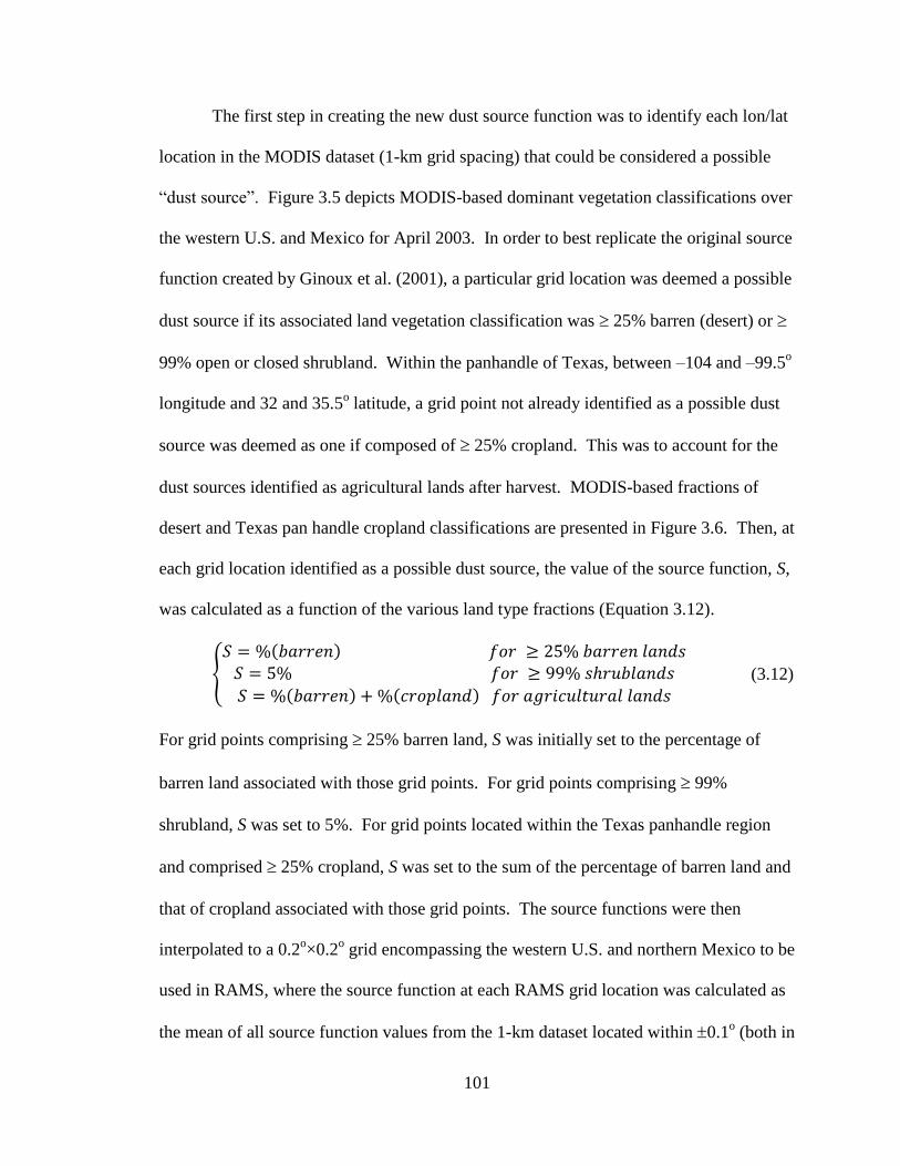
101

The first step in creating the new dust source function was to identify each lon/lat

location in the MODIS dataset (1-km grid spacing) that could be considered a possible

“dust source”. Figure 3.5 depicts MODIS-based dominant vegetation classifications over

the western U.S. and Mexico for April 2003. In order to best replicate the original source

function created by Ginoux et al. (2001), a particular grid location was deemed a possible

dust source if its associated land vegetation classification was 25% barren (desert) or

99% open or closed shrubland. Within the panhandle of Texas, between –104 and –99.5o

longitude and 32 and 35.5o latitude, a grid point not already identified as a possible dust

source was deemed as one if composed of 25% cropland. This was to account for the

dust sources identified as agricultural lands after harvest. MODIS-based fractions of

desert and Texas pan handle cropland classifications are presented in Figure 3.6. Then, at

each grid location identified as a possible dust source, the value of the source function, S,

was calculated as a function of the various land type fractions (Equation 3.12).

{

( )

( ) ( ) (3.12)

For grid points comprising 25% barren land, S was initially set to the percentage of

barren land associated with those grid points. For grid points comprising 99%

shrubland, S was set to 5%. For grid points located within the Texas panhandle region

and comprised 25% cropland, S was set to the sum of the percentage of barren land and

that of cropland associated with those grid points. The source functions were then

interpolated to a 0.2o×0.2

o grid encompassing the western U.S. and northern Mexico to be

used in RAMS, where the source function at each RAMS grid location was calculated as

the mean of all source function values from the 1-km dataset located within 0.1o (both in

102

longitude and latitude) of a particular RAMS grid point. Every RAMS grid point was

assumed to represent approximately the same area, as the ‘dusty’ grid points of interest

were located between 20o and 35

o latitude. Therefore, no cosine (latitudinal) weighting

was performed to create the final source function dataset. Lastly, the RAMS source

function values were adjusted linearly to most closely reproduce the near-surface dust

mass loadings that were observed in the 15-16 April 2003 dust event over western Texas

and eastern New Mexico. This is discussed further in section 7.2.

3.3 Heterogeneous Background Aerosol using WRF/Chem

Atmospheric aerosols interact with each other and undergo complex chemical and

physical transformations. For these reasons, it is difficult to characterize the sources and

sinks of potentially cloud‐active particles with in situ observations. Past treatment of

aerosols in RAMS consisted of initializing the model with some user‐prescribed

horizontally homogeneous profile of aerosol number concentration and size. The aerosol

size and composition remained fixed throughout the simulation and the particle number

field evolved via advection and deposition alone. Andreae and Rosenfeld (2008) argue

that representing the sources and burdens of cloud active aerosol requires a

comprehensive atmospheric model that contains emissions of precursor gases and

primary aerosol species, accounts for transport, transformations, and sinks of precursor

gases, and accounts for the interactions of various aerosol components. Furthermore,

Gustafson et al. (2007) state that a prescribed CCN distribution allowing for vertical and

temporal fluctuations leads to substantially better simulations of cloud properties and

radiative effects as compared to assuming a prescribed uniform and constant CCN

103

distribution. Therefore, RAMS was recently coupled with the Weather Research and

Forecasting with Chemistry (WRF/Chem) model (Grell et al. 2005) to account for the

spatial variability of atmospheric CCN within actual case study simulations (Ward and

Cotton 2011).

Modules within the WRF/Chem framework are used to form a system for

modeling aerosol evolution in the atmosphere, beginning at emission by anthropogenic or

biogenic sources. Anthropogenic emissions of aerosols and aerosol precursor gases are

determined for the continental U.S., southern Canada, and northern Mexico by the

National Emissions Inventory (NEI), which includes both point and area emissions.

Point emissions are released by fixed sources such as power plants, refineries, and other

industrial sites, while area sources represent emissions from sources such as automobiles,

ships, agriculture, and urban activities. Emissions in the NEI have been compiled for

SO2, CO, NOx, NH3, and grouped volatile organic compounds (VOCs). Primary aerosol

PM10 and PM2.5 (particulate matter smaller than 10 and 2.5 µm in diameter, respectively)

emissions are also represented, including sulfate, nitrate, organic, elemental carbon, and

unspeciated aerosol. WRF/Chem uses hourly, summer time representative emissions of

these aerosols, which could lead to inaccuracies for estimates of non‐summer emissions.

The NEI does not account for biomass burning. Natural emissions of aerosol precursor

gases from vegetation are handled by a biogenic emissions module called the Model of

Emissions of Gases and Aerosols from Nature (MEGAN; Guenther et al. 2006). The

module includes emissions of monoterpenes and limonene, needed for biogenic

secondary organic aerosol (SOA) production. MEGAN uses a simple formula for

computing emission rates of various biogenic VOCs using vegetation inventories and

104

estimated canopy information based on leaf area index and foliage conditions. Gas‐phase

chemistry is treated with the Regional Atmospheric Chemistry Model (RACM; Stockwell

et al. 1997). In RACM, organic species with similar oxidation pathways and functional

groups are arranged together in groups. The grouping of organic species corresponds to

the speciation of anthropogenic (16 species groups) and biogenic (3 species groups)

emissions in the NEI. All of these reactions are important in the production of cloud‐

active aerosol since many species need to undergo oxidation in the gas‐phase before

partitioning to the particle phase.

The Modal Aerosol Dynamics Model for Europe (MADE; Ackermann et al.

1998) is used to simulate the aerosol processes and gas‐particle partitioning in

WRF/Chem. Aerosols are separated into three lognormal distributions based on size

(Aitken, accumulation, and coarse modes) and predicted as a single population on

number and size. The Aitken and accumulation modes overlap and interact through

coagulation. Particles are added to the lognormal modes either by direct emission or by

secondary formation. New particle formation is treated solely by the Kulmala et al.

(1998) parameterization of sulfuric acid nucleation, which uses the predicted temperature,

relative humidity, and sulfuric acid vapor concentration to determine a nucleation rate for

particles in the sulfuric acid/water system. New particles are assigned to the Aitken

mode with a diameter of 3.5 nm, and the size distribution parameters are adjusted to

retain the lognormal shape of the distribution. Simulated particles in MADE grow by

condensation and coagulation. Low vapor pressure gas‐phase species condense onto

existing particles at a rate determined by the vapor pressure of the species over the

aerosol surface. The Kelvin effect is parameterized by a size‐dependent growth factor to

105

simplify the computation of the condensational growth rate (Ackermann et al. 1998;

Binkowski and Shankar 1995). Condensation of organic mass is handled by the inclusion

of the Secondary Organic Aerosol Model (SORGAM) into the MADE framework (Schell

et al. 2001). Aerosol mass is predicted for 14 species within the MADE/SORGAM

system (not mineral dust). Aerosol mass can be added to existing particles by

condensation but the particle number remains the same. During coagulation of particles,

the aerosol mass is conserved but the particle number decreases. The lognormal shapes

of the size distributions are held constant in time (Binkowski and Shankar 1995).

Interspecies coagulation occurs in MADE regardless of the particle composition, as the

module assumes internally-mixed aerosol particles composed of multiple aerosol species.

As such, MADE only needs to predict one aerosol number and size distribution that

contains all species.

The WRF/Chem modules simulate the emission and gas to particle formation of

aerosol mass for fourteen separate species, all of which contribute to model CCN. In‐

atmosphere dynamics that modify the particle number and size distribution are also

represented using MADE. The system predicts aerosol mass for each species and one

aerosol size distribution median radius and particle number concentration containing all

species at every grid point. The size and number information can be used directly by the

RAMS droplet activation scheme, but a single‐value representation of the particle

composition using the κ parameter (Petters and Kreidenweis 2007) is still required.

Therefore, the κ parameter is computed as a volume‐weighted average of all 14 aerosol

components and assuming an internal aerosol mixture. This requires values of density for

each WRF/Chem aerosol species or species group to convert the predicted aerosol mass

106

to volume. In addition, a value of κ must be assigned to each component to compute the

weighted average.

WRF/Chem forecasts of aerosol number concentration, mass, size distribution

median radius, and κ are introduced into RAMS using an internal nudging scheme, which

are transported on the RAMS model wind and passed to the droplet activation code. At

each RAMS grid point at a user‐specified time interval, the four aerosol quantities are

updated, or nudged, using Equation 3.13:

( ) ( ) [ ( ) ( )] (3.13)

Pold is the value of a generic variable prior to being updated by the nudging value Pnud,

Pnew is the updated variable, and the nudging factor, nfac, scales the magnitude of the

nudging, preventing large jumps in variable values during the nudging time step. The

four aerosol quantities are nudged for RAMS coarse mode and accumulation mode

aerosols only. Aitken mode particles are not considered to be important to CCN

prediction because of their small sizes. The accumulation mode aerosols are passed

through the RAMS lookup tables. Coarse mode aerosols are not passed through the

lookup tables but are assumed activated at a 100% rate in a supersaturated environment.

WRF/Chem and RAMS use different vertical coordinate systems and often times

different horizontal resolution. Therefore, the WRF/Chem output is linearly interpolated

to that of RAMS offline. Then, if needed, the vertically-interpolated WRF/Chem data are

linearly interpolated to the RAMS grid in the horizontal (also offline). In between

nudging time steps, particles in RAMS are advected by the model wind. However,

neither aerosol dynamics nor chemical processes, including emissions, are treated.

Therefore, it is recommended that aerosol variables within RAMS be tightly constrained

107

by the WRF/Chem forecasts using a high nudging factor (nfac=0.2) and high nudging

frequency (every 5 minutes).

One should note the multiple limitations to the WRF/Chem-RAMS coupling

methodology. Some have already been stated. In addition, recall that the

MADE/SORGAM and chemical mechanism modules within WRF/Chem predict the

major known components of ambient CCN using a modal representation of aerosols.

McKeen et al. (2007) found that WRF/Chem forecasts of PM2.5 distributions exhibited a

low bias in rural areas, attributed to the inadequate treatment of SOA formation and the

lack of consideration of some biogenic precursor gases. The modal representation of

aerosol size distribution, while reducing computation time, also precludes our ability to

simulate complex size distributions and size‐dependent composition. These complexities

affect the cloud‐active fraction of a predicted aerosol (Abdul‐Razzak and Ghan 2002).

Another limitation is the lack of aqueous‐phase sulfate production within the WRF/Chem

module (Kanakidou et al. 2005). Differences in meteorology and cloud processes

between WRF/Chem and RAMS predictions could also lead to inconsistencies in the

aerosol fields, a clear disadvantage of running the aerosol code offline with respect to

RAMS. This becomes especially important in precipitating regions where aerosol

scavenging occurs. Wet deposition is not represented in WRF/Chem, which could lead to

underestimates of total deposition rates in some areas and overestimates of the aerosol

burden. Therefore, even if RAMS correctly removes particles from the atmosphere

during a precipitation event, the nudging constrains the aerosol to possibly inaccurate

WRF/Chem output. Despite these limitations, the aerosol coupling between WRF/Chem

output and RAMS allows for the prediction of CCN and cloud droplet number

108

concentration (CDNC) in RAMS based on model estimates of aerosol properties,

including composition. By integrating the WRF/Chem output and RAMS, even offline,

CDNC predictions in RAMS represent the temporal and spatial variability of the ambient

aerosol.

3.4 Dust Microphysics Activation

The concept of mineral dust having the potential to serve as CCN, GCCN, and IN

was covered at length in Chapter 2. With dust emissions now included in RAMS using

the Ginoux et al. (2001) dust source model (Smith 2007), parameterizations were

developed for simulating dust microphysical effects within the RAMS microphysical

routines. However, multiple factors were considered with respect to the activation of

model dust as CCN, GCCN, and IN, including accounting for the competition effect,

separating the dust size distribution into potential CCN and GCCN, deciding what

fraction of the dust population may serve as IN, and how to treat nucleation scavenging

(wet deposition) as potential sinks of dust.

3.4.1 Activating Dust as CCN

This section describes the creation of a realistic and computationally efficient

algorithm for activating mineral dust as CCN within RAMS given an externally-mixed

total aerosol population, which includes fine mode mineral dust from the dust scheme and

pre-existing background (non-dust) accumulation mode particles from WRF/Chem.

Making the accumulation mode dust particles cloud-active is challenging, as these

aerosols have different size distribution median radii than the WRF/Chem predicted

109

aerosols; they are typically larger. Moreover, their chemical composition differs

appreciably from say anthropogenic pollution aerosols. Since the droplet activation

scheme in RAMS (Saleeby and Cotton 2004, 2008; Ward et al. 2010) predicts droplet

number from a single mode aerosol distribution, inter-modal competition for water vapor

would not be treated if multiple modes were considered separately within the scheme.

Therefore, a scheme for combining two aerosol size distributions into one, in such a way

that the droplet activation properties of both modes are retained, was implemented for

these applications. Two sets of numerical simulations were performed using a parcel

model, in which aerosol populations composed of both dust and non-dust aerosol

mixtures were allowed to activate cloud droplets under multiple environmental

conditions, wherein the competition effect amongst the different aerosol distributions was

included. The methods presented herein were used to create a dust-CCN activation

lookup table to account for the presence of lofted dust in future RAMS simulations.

This study makes use of a Lagrangian parcel model (Heymsfield and Sabin 1989),

described by Saleeby and Cotton (2004). The model activates cloud droplets within an

air parcel containing an initial lognormal dry aerosol distribution and determines the

fraction that serves as CCN given a particular environment. The aerosol distribution is

based on a prescribed size distribution median radius and shape parameter and broken

into 100 size bins. The parcel is lifted with an initial updraft velocity, wherein it becomes

supersaturated with respect to water. Activation of haze particles and droplet growth in

each size bin, and changes in temperature, pressure, air density, and liquid water content

with time are solved iteratively with the Variable-coefficient Ordinary Differential

Equation (VODE) solver (Brown et al. 1989). The model activates haze and cloud

110

droplets via liquid-phase condensation only. It does not allow for ice microphysics or

sedimentation. The independent variables (initial conditions) include the initial aerosol

number concentration, or number concentration of condensation nuclei (NCN), aerosol

size distribution median radius (rg), initial updraft velocity (w), parcel temperature (T),

and aerosol hygroscopicity (Eidhammer et al. 2009) using the hygroscopicity parameter,

(Petters and Kreidenweis 2007).

The parcel model assumes a single lognormal distribution composed of a single or

internally-mixed, aerosol species, as numerically modeling externally-mixed aerosols is

admittedly difficult. While this assumption can yield both over- and under-predictions of

CCN, the mixing state of most ambient aerosol can be considered at least quasi-internal

(e.g., Rissman et al. 2004; McFiggans et al. 2006; Ervens et al. 2007; Cubison et al.

2008). Background aerosol concentrations in RAMS are assumed to be composed of

internally-mixed aerosol particles and represented by a single value of . However,

mineral dust concentrations are treated separately to those of non-dusty (background)

aerosol concentrations. Therefore, two sets of numerical simulations using the parcel

model were performed for this study, each consisting of 28,800 individual parcel

simulations that encompass a variety of initial environmental conditions and aerosol

populations. Values of the independent variables utilized in these simulations are

displayed in Table 3.3. Dust was assumed to originate from the southwestern U.S.,

assigned a value of 0.03 (Koehler et al. 2009) and an accumulation mode median radius

of 0.2 µm. The value of 0.03 was taken from the results of Koehler et al. (2009), who

derived the value using dry-generated Arizona Test Dust (ATD, grade A2), a

commercially-produced, milled product (Powder Technologies, Inc.) originating from

111

Arizona sand, often used to represent North American soil (Koehler et al. 2009; Kumar et

al. 2011). Background values of were varied between 0.05 and 1.0 in order to account

for most typical internally-mixed aerosols. Note that NaCl possesses a value of 1.28

(Petters and Kreidenweis 2007). Andreae and Rosenfeld (2008) reported that typical

continental values of range between 0.2 and 0.4, with few observations below 0.1. The

lognormal shape parameter, g, was fixed at a value of 1.8 to maintain consistency with

existing RAMS lookup tables (Saleeby and Cotton 2004; Ward et al. 2010). The initial

pressure and relative humidity were also constant for all simulations (600 mb and 99%,

respectively) for the same reason. The dust median radius and κ were held constant in

the parcel simulations as well, because they are constant in the RAMS dust source and

transport module.

In the first ensemble, dust and background aerosol distributions were added to

create one bimodal distribution. The parcel model initialization required that the dust and

background distributions be represented by a single value of . Therefore, following the

methods described in Petters and Kreidenweis (2008), each dust bin in the initial

prescribed dust distribution was resized to an effective radius, corresponding to the size

that particle would be if it were forced to comprise the same composition (and thus

hygroscopicity) as that of the background aerosol. The dust distribution, defined by the

effective radius, was added to the background aerosol distribution. The parcel model was

then run with this combined aerosol distribution, assuming the background value of .

Results from various sensitivity tests indicated that this method yields realistic CCN

activation (Daniel Ward, personal communication). Therefore, this set of simulations

112

will be referred to as the ‘control’ (CTL) ensemble, the results from which will be

considered as “truth”.

In the second set of simulations, the background aerosol and dust distributions

were combined into one single mode lognormal distribution using the methods described

below. The combined distribution was represented by a single value of rg, NCN, and ,

where rg and were dependent on the total mass of both aerosol concentrations. The

mass of the background (mb) and that of the dust (md) were calculated using Equation

3.14:

2/exp3

4 3

xxgxx Nrm (3.14)

mx is the mass, rgx is the size distribution median radius, Nx is the CN concentration, and

x is the density of the aerosol species, x. Then the bulk size distribution median radius

could be calculated using Equation 3.15.

3/1

)2/exp()(4

3

d

d

b

b

db

g

mm

NNr

(3.15)

The subscripts ‘b’ and ‘d’ represent values corresponding to the background and dust

distributions, respectively. b was held fixed at 1.77 g cm-3

. d was assumed to be 2.65 g

cm-3

. Equations 3.14 and 3.15 are based on Equation 10 from Saleeby and Cotton

(2004). The bulk value of was calculated using Equation 3.16.

d

d

b

b

d

d

db

b

b

mm

mm

(3.16)

The total CN concentration (NCN) was calculated as the sum of Nb and Nd. The parcel

model was run, representing the single lognormal aerosol distribution with the newly

113

calculated bulk values of rg, NCN, and . These simulations will be referred to as the

experiment (EXP) ensemble. The activated CCN concentrations were compared between

the CTL and EXP ensembles, and a dust activation lookup table was constructed that

forced the EXP activated CCN concentrations to most closely match those of the CTL

ensemble.

Figure 3.7 displays a scatter plot comparing activated CCN between the CTL and

EXP parcel ensembles, where each open circle represents one of the 28,800 pairs of

parcel simulations. A simulation pair refers to any set of CTL and EXP simulations

initiated with the same initial conditions. The one-to-one line is overlaid. The EXP

simulations severely overestimated CCN activation in general, often times by more than

an order of magnitude. Percent errors, calculated as the absolute value of the quantity

[(NCCN,EXP – NCCN,CTL) / NCCN,CTL]x100%, were determined for every simulation pair. The

mean and maximum percent errors over the full dataset were 27% and 908%,

respectively. Of the 28,800 individual parcel model simulations, 25,710 of them

overestimated the activated CCN concentration in the EXP setup compared to

corresponding CTL simulations. This was due primarily to two causes. First, when the

median size of the dust was larger than that of the background, combining the dust and

background aerosol concentrations into one evenly-mixed, mass-weighted lognormal

distribution overly skewed the bulk median radius toward that of the larger dust particles,

making the smaller particles in the distribution large enough to serve as CCN given the

bulk value of . Secondly, as the background aerosol concentration was increased in a

particular set of EXP simulations, the bulk value of in the combined lognormal

distribution increased and the median radius decreased. Decreasing the median size of

114

the aerosol population alone reduced the likelihood of the smallest particles being large

enough to serve as CCN. However, the associated increase in was often great enough

to activate too large a fraction of the aerosol population compared to that in the

corresponding CTL simulation.

Various relationships were discovered within the model parameter space of the

two model ensembles, making it possible to adjust the often over-activated CCN

concentrations in the EXP simulations towards the concentrations produced in the CTL

simulations. Figure 3.8a displays CTL versus EXP activated CCN for a specific set of

parcel simulations where vertical velocity, κ, parcel temperature, and dust number

concentrations were held constant. In this case, w=0.361 m s-1

, b=0.6, T=10oC, and

Nd=316 cm-3

. The EXP-activated CCN failed to match those from the corresponding

CTL simulations, especially when CTL-activated CCN concentrations varied between

100 and 500 cm-3

. However, when the median aerosol size ratio was plotted against

corresponding values of CCN activation ratio (NCCN,CTL/NCCN,EXP) for this specific subset

(Fig. 3.8b), it became evident that each specific aerosol size ratio was associated with a

range of CCN activation ratios. In addition, a geometric relationship was calculated

linking the aerosol concentration ratio (Nrat, defined as Nd/Nb) to the CCN activation

ratio. Examples of this are shown in Figure 3.8c-d for two aerosol median size ratios.

When the aerosol concentration ratio was plotted versus CCN activation ratio for parcel

simulations where the aerosol size ratio was equal to 0.4 (data points in between the two

dashed vertical lines in Fig. 3.8b), the CCN activation ratio varied little with aerosol

concentration ratio (Fig. 3.8d). A best-fit geometric relationship of the form y=axb+c was

calculated nonetheless (Fig. 3.8d, overlaid curve), where y is CCN activation ratio and x

115

is aerosol concentration ratio. When the aerosol size ratio was equal to 0.05 (data points

in between the two solid vertical lines in Fig. 3.8b), the geometric relationship fitted to

the plotted data points (Fig. 3.8c, overlaid curve) was given by a=0.3022, b=0.4197, and

c=0.3653. This curve revealed that the CCN activation ratio increased with increasing

aerosol concentration ratio. This meant that increasing the background aerosol

concentration, given a particular cloud environment and dust concentration, generally

increased the number of activated CCN in the EXP simulation compared to the

corresponding CTL parcel simulation for reasons previously discussed. Similar

geometric relationships were found consistently for every data subset, meaning that for

the aerosol size ranges considered in this study (Table 3.3), aerosol particle size and

composition played important roles in determining a particle’s ability to act as a nucleus

for cloud droplet activation.

Determining the geometric relationships that related aerosol concentration ratio to

CCN activation fraction for every particular ensemble subset allowed the construction of

a lookup table that provided CCN activation ratio as a function of the vertical velocity,

the aerosol concentration ratio, dust number concentration, background hygroscopicity

parameter κ, parcel temperature, aerosol median size ratio, aerosol concentration ratio,

and dust number concentration. For every combination of these variables (Table 3.3),

corresponding geometric best-fit values a, b, and c were included in the lookup table,

thus relating each bulk single mode lognormal aerosol distribution-based activated CCN

concentration to a tuned value.

To test the accuracy of the lookup table, a final (tuned) activated CCN

concentration was calculated by multiplying the EXP concentrations by their

116

corresponding CCN activation fractions via use of the lookup table. The scatter plot in

Figure 3.9 displays CTL activated CCN concentrations versus those of the tuned EXP

simulations, where every EXP parcel simulation was put through the process just

described, thus creating a tuned activated CCN concentration for every parcel simulation

from the EXP runs using the lookup table. More of the data points fall much closer to the

one-to-one line compared to Fig. 3.7. Only 50 of the tuned EXP simulations activated the

same CCN concentration as their corresponding CTL simulations. However, 14,091 of

the tuned EXP simulations overestimated activated CCN concentrations compared to the

CTL simulations, and 14,659 simulations underestimated the activated CCN. This

indicates that the tuned EXP activated CCN were not skewed toward over activation.

Factoring in all 28,800 simulation pairs from the tuned EXP and CTL ensembles yielded

a correlation coefficient of 0.9994. The associated mean and maximum percent errors

were only 2.43% and 34.96%, respectively, a major improvement compared to the CCN

activations in the original EXP ensemble. Use of the activation lookup table greatly

reduced the overestimation of activated CCN that occurred in the original EXP

simulations.

Note that two more sets of parcel simulations using the same parameters listed in

Table 3.3 were performed, but for a constant dust median radius of 0.7 µm. The

simulations yielded similar results to those assuming a dust median radius of 0.2 µm.

Figure 3.10 displays a scatter plot comparing activated CCN between the CTL and EXP

parcel ensembles. The over-activation of CCN in the EXP simulations is even more

apparent, but geometric relationships were again successfully calculated that linked Nrat

to the CCN activation ratio (not shown). These relationships led to the creation of a CCN

117

activation lookup table based on a dust median radius of 0.7 µm. Tuned activated CCN

concentrations were again calculated using the methods described previously, and the

results are displayed in Figure 3.11. Factoring in all 28,800 simulation pairs from the

tuned EXP and CTL ensembles improved the correlation coefficient from 0.929 to

0.9997. The associated mean and maximum percent errors improved from 31% and

175% to 3.87% and 75.3%, respectively.

3.4.2 Activating Dust as GCCN

The lookup table-based droplet activation scheme in RAMS is set up to predict

droplet number on only a single aerosol distribution for every grid cell and time step.

Since Aitken mode aerosols are not likely to be as important in CCN prediction as those

of the accumulation mode, accumulation mode aerosol distributions are used in the CCN

activation scheme. This means that coarse mode aerosols with the potential to serve as

GCCN may not be passed through the droplet activation scheme. Instead, the coarse

mode distributions have traditionally been assumed to have the chemical properties of sea

salt, thus activating at a 100% rate in a supersaturated environment (Saleeby and Cotton

2004). This same philosophy has been adopted for activating the coarse mode aerosol

distributions predicted from WRF/Chem (Ward and Cotton 2011).

The assumption that all available GCCN are activated upon saturation is defended

by the fact that GCCN are defined as particles with radii typically larger than 1 µm.

Recall from the discussion of the Köhler equations in Chapter 2 that for a given chemical

composition, as the dry particle size increases, the critical supersaturation decreases,

making it is easier to activate larger particles. This is because for very large dry aerosol

118

particles, the size of the droplet at activation is very large, and thus the Kelvin (curvature)

effect is very small. Therefore, if a dry particle is large enough to be considered a

GCCN, it can be nearly insoluble and still activate at reasonable supersaturations. It

therefore might seem feasible to simply allow all coarse mode dust particles predicted by

RAMS to act as potential GCCN, considering that the coarse mode dust particles in

RAMS are typically larger than those making up the background distributions. However,

the WRF/Chem-based aerosols produced in RAMS may possess values of κ (often equal

to or greater than 0.3) that are an order of magnitude larger than that attributed to dust (κd

assigned a value of 0.03). Therefore, another ensemble of parcel simulations was

performed using the parcel model of Heymsfield and Sabin (1989) in order to assess the

ability of mineral dust to serve as GCCN. The parcel model (described in section 3.4.1)

was initiated with a single mode lognormal aerosol distribution using a κ value of 0.03 to

represent dust. 735 parcel simulations were performed, encompassing a variety of

particle sizes, initial environmental conditions, and aerosol populations. Values of the

independent variables utilized in these simulations are presented in Table 3.4. The initial

temperature was held fixed at 10oC for simplicity and to reduce simulation time. Just as

in the previous parcel simulations (section 3.4.1), g was fixed at a value of 1.8, the

initial pressure was 600 mb, and the initial relative humidity was 99%. Note that these

large particles rarely reach their expected equilibrium radius given normal cloud liquid

water contents. However, this is assumed in the parcel model.

Figure 3.12 displays dust GCCN activated fractions, defined by the quantity

NdCCN/NTOT, as a function of vertical velocity on a log10 scale for each parcel simulation.

There is a wide spread of activation fractions at vertical velocities ≤ 1 m s-1

. However, it

119

is evident that a particle’s ability to serve as a GCCN generally increases with increasing

vertical velocity. Furthermore, a 3rd

order polynomial was fitted to the data, relating dust

GCCN activation fraction to updraft speed for vertical velocities between 0.01 m s-1

and

10 m s-1

. The polynomial is of the form

(3.17)

where y represents NdCCN/NsCCN, x denotes the log10 quantity of the vertical velocity, and

the five ‘a’ terms are coefficients. A 3rd

order polynomial equation was chosen, because

it was the lowest order polynomial that could represent the vertical velocity dependence

on activation while most improving upon the correlation coefficient of the next lowest

order polynomial fit (correlation coefficients of the data with the best fit 2nd

, 3rd

, 4th

, and

5th

order polynomial equations were 0.878, 0.882, 0.882, and 0.872, respectively). In this

case, a0=0.918, a1=0.251, a2= –0.136, and a3= –0.040. Note that this relationship is only

valid when the updraft speed is between 0.01 m s-1

and 10 m s-1

, and the best-fit

activation fraction reaches a value of 1.0 at 2.87 m s-1

. For vertical velocities less than

0.01 m s-1

, the dust activation fraction will be held constant at a value of 0.192 (the value

associated with a vertical velocity of 0.01 m s-1

). For updrafts greater than 2.86 m s-1

,

100% of the coarse mode dust may activate as GCCN, corresponding to a dust activation

fraction of 1.0. This way, the activation potential of the coarse mode dust as GCCN in

RAMS will be determined as a function of ambient vertical velocity. For example, if the

vertical velocity at a particular time step and grid cell is 1 m s-1

, then (from Fig. 3.14) just

over 92% of the corresponding coarse mode dust population will be added to the

background potential GCCN array to be used for cloud2 droplet nucleation.

120

3.4.3 Activating Dust as IN

DeMott et al. (2010) presents a relatively simple parameterization for activating

mineral dust and other aerosol as IN within mixed-phase clouds in a numerical model.

This parameterization has been implemented in RAMS for use in this study. While

advances in the understanding of atmospheric sources, transformations, and sinks of IN

have been limited, the DeMott et al. (2010) scheme is based on observed relationships

between aerosols and IN populations from eight observational datasets collected within

the past decade, primarily with respect to aerosol size and cloud temperature. Note that

aerosol composition was not examined specifically. IN data were from the Colorado

State University Continuous Flow Diffusion Chamber (CFDC), which processed aerosol

particles from ambient air samples to determine the IN number concentrations present for

specific temperature and humidity conditions. Aerosol data were collected from

condensation particle counters and from mobility, optical, and aerodynamic particle

sizing (APS) instruments. Aerosol aerodynamic diameter data from the APS were

corrected to physical diameter, based on an assumed average dust particle density of 2.3 g

cm-3

. Aerosol and IN concentrations were corrected to standard temperature and pressure

conditions (STP; 273.15 K, 1013.25 mb).

DeMott et al. (2010) found that the number concentrations of aerosol particles

exceeding approximately 0.5 µm in diameter was a strong predictor of IN concentrations,

while cloud temperature played an important but secondary role. The overall size and

temperature dependencies of IN active under mixed-phase cloud conditions are

represented by Equation 3.18 (Equation 1 from DeMott et al. 2010),

( )

( )( ( ) )

(3.18)

121

where a=0.0000594, b=3.33, c=0.0264, d=0.0033, Tk is cloud temperature in Kelvin,

naer,0.5 is the number concentration (scm-3

) of aerosol particles with diameters larger than

0.5 µm, and is ice nuclei number concentration (std L

-1) at Tk. This

parameterization is based at STP. Therefore, all aerosol number concentrations must be

converted to STP in order to calculate activated IN, then the IN concentrations must be

converted back to the temperature and pressure of the ambient cloud environment.

Figure 3.13 shows activated IN concentrations as a function of both potential IN aerosol

concentrations and temperature according to the DeMott et al. (2010) scheme.

The DeMott et al. (2010) parameterization is based only on IN concentrations

measured at relative humidity with respect to water exceeding 100% (101-104%), where

contributions from all known ice nucleation mechanisms are possible, including

deposition nucleation, condensation-freezing, and immersion freezing. The scheme is

therefore not valid for relative humidity with respect to water below saturation. This

limitation is not likely an important factor when numerically simulating a supercell

thunderstorm. DeMott et al. (2010) believe that their measured IN number

concentrations reflect the maximum ambient IN number concentrations due to the

combined action of all known mechanisms at temperatures below about –35oC.

3.4.4 Scheme Implementation, Benefits, and Limitations

A dust microphysical activation scheme has been implemented into RAMS,

which emulates the effectiveness of mineral dust to serve not just as one nucleation

species, but as CCN, GCCN, and IN. A flow chart summarizing the dust microphysics

scheme is shown in Figure 3.14. The dust-CCN activation lookup table uses only those

122

dust concentrations in the accumulation mode, accounting for the water vapor

competition effect but assuming that the dust becomes internally-mixed with the

background aerosol population pre-activation. The lookup table utilizes a constant dust

median radius and κ and assumes the presence of two individual lognormal aerosol

distributions, one of pure dust and one representing the total population of all non-dust

particulates. Recall that RAMS utilizes preexisting lookup tables within its cloud droplet

activation scheme along with WRF/Chem-based aerosol data, represented by a lognormal

distribution, defined by the total number concentration, total mass, and mass-weighted

values of size distribution median radius and κ. These aerosol quantities, representing the

background aerosol population, are nudged for RAMS accumulation mode and coarse

mode aerosols, of which the accumulation mode aerosols are used to activate CCN. In

future numerical experiments that include the added presence of lofted dust, RAMS may

activate CCN by combining the dust and background lognormal aerosol distributions into

one bulk, mass-weighted lognormal distribution, represented by the total number

concentration, NCN, total mass, and mass-weighted values of size distribution median

radius, rg, and κ. This bulk lognormal distribution will be run through the cloud droplet

activation scheme to produce some activated CCN concentration. However, before the

activated CCN concentration is utilized further in RAMS microphysical routines, the new

dust activation lookup table will be called. The grid-cell vertical velocity, κ, air

temperature, median aerosol size ratio, aerosol concentration ratio, dust number

concentration, and total aerosol number concentration will be matched to the most

representative set within the lookup table to assign best-fit geometric values of a, b, and c

to the grid cell. These values will then tune the original activated CCN concentration to a

123

more realistic value. It is this final activated CCN concentration that will be used further

within the RAMS model microphysics.

GCCN activation from dust in RAMS is not based on the activation lookup tables

but rather the assumption that some fraction of the coarse mode dust (dependent on

vertical velocity) may activate at a 100% rate in a supersaturated environment in a

specific grid cell at a particular time, following the results of the coarse mode dust parcel

model simulations.

The activation of dust as IN complicates matters, as dust particles from both the

fine and coarse modes may realistically have the potential to activate IN (particle

diameters > 0.5 µm). The scheme is further complicated by the size overlap of the two

modes. In this study, the fine and coarse mode dust distributions are prescribed median

radii of 0.2 µm and 2.65 µm, respectively, based on limited observations of the case

study of interest (presented in Chapter 7). Assuming a lognormal distribution for both

modes, only 0.34% of the particles in mode 1 have radii greater than 1 µm, thus able to

potentially serve as GCCN. Therefore, none of the fine mode distribution will be used as

potential GCCN. However, 37.82% of the particles in the distribution have diameters

larger than 0.5 µm and are thus potential IN. 4.5% of the particles in the coarse mode

distribution have radii smaller than 1 µm and thus could serve as CCN. However, since

mode 2 number concentrations are rather small (usually no more than a few per cubic

centimeter), none of the coarse mode distribution will be allowed to serve as CCN. On

the contrary, the entire (99.998% of the) coarse (mode 2) distribution are of sufficient

size and therefore allowed to serve as IN in the DeMott et al. (2010) scheme.

124

The DeMott et al. (2010) scheme is not dependent upon aerosol composition but

rather calculates pristine ice concentrations based on the total aerosol number

concentration of particles greater than approximately 0.5 µm in diameter. Therefore, the

potential IN concentration to be used in Equation 3.18 within RAMS comprises the

background CCN and GCCN populations in addition to any existing concentrations of

dust. Therefore, dust concentrations are partitioned as potential CCN and GCCN versus

IN as a function of temperature by first addressing dust as potential IN, even though the

activation of CCN and GCCN occur prior to that of IN in RAMS. Figure 3.15 displays

IN activation fractions, defined as the ratio of the activated aerosol or pristine ice number

concentration (NPI) by the initial potential IN aerosol concentration (Na), as a function of

temperature at 0.5oC increments, for a variety of initial potential IN aerosol

concentrations (calculated using Equation 3.18). Notice that the scheme does not activate

IN at temperatures at or above 0oC. At temperatures between –55

oC and 0

oC, less than

50% of the initial aerosol population is used to nucleate ice crystals. This suggests that at

warmer temperatures where warm-rain processes are most likely to occur, very few

aerosol particles that could potentially serve as IN would actually be used for ice

nucleation in the DeMott et al. (2010) scheme. Therefore, lofted dust in RAMS is

discriminated into potential CCN, GCCN, and IN as follows, recalling that roughly 38%

of the fine mode dust distribution is of sufficient size to serve as IN. First, the potential

IN concentration is calculated as the sum of the background CCN population greater than

0.5 µm (based on the relationship between lognormal median radius and fraction of

population greater than 0.5 µm), 100% of the background GCCN population, 38% of the

mode 2 dust, and 100% of the mode 2 dust concentrations. This total number

125

concentration and associated temperature and pressure are converted to STP, where

Equation 3.18 can be used to calculate the activated IN concentration. This activated

concentration is then converted back to ambient temperature and pressure. The potential

IN concentration is saved, then used in the ice microphysics routine, but the fraction of

the potential IN concentration left un-activated will be allowed to potentially serve as

CCN and GCCN. Activated IN concentrations are first assumed to be comprised of

mode 2 dust, then background GCCN, then mode 1 dust, then background CCN. This is

based on the assumption that Equation 3.18 will activate the largest IN for ice nucleation.

Once the partitioning of dust as potential CCN, GCCN, and IN is complete, any

mode 1 dust that fails to nucleate pristine ice may serve as CCN using the RAMS CCN

activation scheme and associated lookup tables. Note that even though the larger

particles in the distribution are potentially used for IN activation, the remaining fine

mode dust used in the CCN activation scheme will still assume a lognormal distribution

represented by the original median radius. In reality, a smaller median radius should be

used, and assuming a lognormal size distribution may no longer be appropriate.

Nevertheless, a lognormal distribution represented by the original median size will be

used to maintain simplicity and consistency with the dust-CCN activation lookup table.

If a mode 2 dust population remains after the calculation of the number

concentration to serve as IN, then most of this remaining mode 2 number concentration

will be used for GCCN activation. Recall that 4.5% of particles in mode 2 are too small

to serve as GCCN. Therefore, 4.5% of the available mode 2 population will be

subtracted from the available distribution, and it is this final number concentration (if

greater than zero) that may be used to serve as GCCN. Then, vertical velocity must be

126

considered. Equation 3.17 determines the maximum fraction of the coarse mode dust

population that is allowed to serve as GCCN. Therefore, the ratio of the mode 2

population left available to serve as GCCN to the total mode 2 dust population will be

compared to the activation fraction calculated by Equation 3.17. The minimum of these

two fractions will determine the number of mode 2 dust that will be added to the potential

GCCN array for the activation of cloud2 droplets. Once CCN and GCCN activation have

occurred within RAMS, then the previously calculated activated IN population will be

added to the pristine ice category, based on available supersaturations with respect to ice.

Use of the DeMott et al. (2010) IN activation scheme requires two adjustments.

First, the measurements from which Equation 3.18 is based made use of optical sizing to

differentiate observed ice crystals from water drops and aerosol particles required the use

of an impactor system upstream of the CDFC to limit sampled particles to aerodynamic

sizes less than 1.6 µm. As a result, the DeMott et al. (2010) scheme does not account for

particles with diameters greater than 1.6 µm that might serve as IN. This means that the

scheme under-predicts activated IN concentrations in environments such as dense mineral

dust plumes, which are defined by high concentrations of potential IN greater than 1.6

µm diameter. Recent testing of the scheme’s accuracy in such environments led to the

findings that (i) when aerosol concentrations greater than 0.5 µm in diameter are near or

less than 70 cm-3

, Equation 3.18 will under-predict activated IN concentrations by a

factor of five, based on measurements at –25oC and (ii) when number concentrations

greater than 0.5 µm in diameter are in excess of 70 cm-3

, Equation 3.18 under-predicts

activated IN concentrations by a factor of 10, based on measurements colder than –35oC

(Paul DeMott, personal communication). Therefore, when RAMS predicts such aerosol

127

concentrations, the activated IN concentrations (and thus pristine ice populations) must

be nudged by a factor of five or 10, accordingly. Second, looking back at Fig. 3.15, it is

clear that at temperatures colder than –62oC, the scheme actually activates a greater

population of aerosol as IN than originally available. For relatively large number

concentrations of potential IN and cold temperatures, the parameterization over-activates

IN by factors of five and greater. As a result, a check must be performed so that the

number of activated IN may not exceed that of the potential IN aerosol concentration.

The treatment of aerosol nucleation sources and evaporation sinks in RAMS are

nontrivial issues. RAMS contains a relatively simple source/sink scheme for CCN and

GCCN, where aerosols are removed after droplet nucleation via nucleation scavenging

and replenished upon droplet evaporation. This scheme was expanded upon in order to

include the presence of dust. Activating dust as CCN requires adding together the

background aerosol and dust into a single array of potential CCN pre-activation and it is

not possible after activation to back out the number concentration of dust that served as

CCN versus that which did not. However, CCN activation in a particular grid cell at a

particular time is calculated online within RAMS twice: first using mode 1 dust as

additional CCN, then using only the background CCN population. If the added presence

of dust increases the number of cloud1 droplets nucleated, then the difference is

subtracted from the mode 1 dust population. The remaining activated population is

subtracted from the background CCN concentration. Activated cloud 2 droplets are first

assumed to originate from mode 2 dust serving as GCCN, then the background GCCN

population, again based on the assumption that the largest particles nucleate first. After

nucleation, the number of nucleated cloud2 droplets is subtracted from the mode 2 dust

128

and background GCCN concentrations, accordingly. Upon droplet evaporation, the

numbers of cloud1 and cloud2 droplets evaporated are added directly to the background

CCN, and GCCN populations, respectively. Cloud droplet evaporation does not

contribute to the dust concentrations.

Treating ice nucleation scavenging as a sink for dust and background aerosol

concentrations has also been implemented in RAMS based on the assumption that larger

particles nucleate ice before smaller particles. After the calculation of nucleated pristine

ice crystal concentration in a grid cell at a particular time step based on available

supersaturations with respect to ice, the newly added pristine ice population is subtracted

from the mode 2 dust concentration, then the background GCCN population, then the

mode 1 dust, and finally from the background CCN. Sublimation does not act as an

added source of IN. Potential IN concentrations are calculated every time step using the

background CCN and GCCN populations along with the mode 1 and mode 2 dust

concentrations.

129

Table 3.1: Median radius and mass fraction for binned dust source function.

Bin 1 2 3 4 5 6 7

Radius (µm) 0.15 0.265 0.471 0.831 1.5 2.65 4.71

Mass fraction 0.0009 0.0081 0.0234 0.0676 0.3 0.3 0.3

130

Table 3.2: IGBP Land Cover Units (Table 1 from Strahler et al. 1999).

131

Table 3.3: Initial values of the independent variables used in the parcel model simulations

Constants d = 0.03 rd = 0.2 m, 0.7 m

T (oC) -5 10 25

w (m/s) 0.01 0.0361 0.361 1.0 3.61 10.0 30.0

b 0.05 0.2 0.6 1.0

Nb (cm-3

) 100 316 1000 3160 10000

rb (m) 0.01 0.02 0.04 0.06 0.08 0.12 0.2 0.4 0.6 1.0

Nd (cm-3

) 31.6 100 316 1000 2000

132

Table 3.4: Initial values of the independent variables used in the GCCN parcel model

simulations.

Constants T=10oC κ=0.03

w (m/s) 0.01 0.0361 0.361 1.0 3.61 10.0

N (cm-3

) 0.1 0.5 1.0 5.0 10.0

rg (m) 2.5 3.0 3.5 4.0 4.5 5.0 5.5

133

Figure 3.1: The Ginoux et al. (2001) dust source function, S, over the western U.S. and

Mexico. The colorbar denotes nondimensional values of S.

134

Figure 3.2: Map outlining the Chihuahuan Desert (after Schmidt 1979; from Rivera

Rivera et al. 2009).

135

Figure 3.3: Fraction of the desert category derived from (a) USGS land-cover data and

(b) MODIS land-cover data (adapted from Park et al. 2009).

136

Figure 3.4: MODIS images of dust plumes originating over northwestern Texas and

eastern New Mexico on (a) 15 December 2003, (b) 1 January 2006, (c) 24 February 2007,

and (d) 6 April 2006 (Figs 3.4a-c from http://earthobservatory.nasa.gov; Fig. 3.4d from

http://visibleearth.nasa.gov)

(c)

(a) (b)

(d)

137

Figure 3.5: Dominant vegetation classifications derived from the MODIS land cover

product for April 2003, generalized and grouped in six primary land type classifications:

savannas (SAV), croplands (CRP), grasslands (GSL), shrub lands (SHB), forest (FST),

and desert or barren land (DST).

138

Figure 3.6: MODIS-based fractions (percentages) of barren land, or desert, category

(yellow-oarange-red colorbar) and croplands within the Texas panhandle (blue-green

colorbar). Fractions are given in units of percent.

139

Figure 3.7: Activated CTL CCN (cm

-3) vs. activated EXP CCN (cm

-3) for all parcel

model simulations. The black line represents the one-to-one line where CTL CCN is

equal to that of EXP CCN for the same initial conditions.

140

Figure 3.8: Plots of (a) CTL vs. EXP activated CCN (cm

-3) and (b) median aerosol size

ratio vs. CCN activation ratio for w=0.361ms-1

, b=0.6, T=10oC, and Nd=316; (c) aerosol

number concentration ratio vs. CCN activation ratio for an aerosol size ratio 0.05, shown

as the data points surrounded by the two solid vertical lines in Fig. 3.8b; (d) same as (c)

but for an aerosol size ratio of 0.4, shown as the data points in between the two dashed

vertical lines in Fig. 2b. The black line in Fig. 3.8a represents the one-to-one line. The

curves overlaid on Fig. 3.8c-d represent the best-fit geometric curves to the plotted data,

represented by the parameters a, b, and c.

141

Figure 3.9: Same as Fig. 3.7 but for CTL vs. lookup table-tuned EXP activated CCN

(cm-3

).

142

Figure 3.10: Same as Fig. 3.7 but for a dust median radius of 0.7 µm.

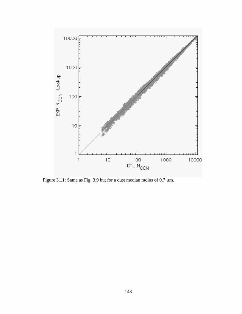
143

Figure 3.11: Same as Fig. 3.9 but for a dust median radius of 0.7 µm.

144

Figure 3.12: Dust GCCN activation fractions plotted as a function of vertical velocity for

each parcel simulation. The black curve represents the 3rd

order polynomial best-fit curve

to the dataset.

145

Figure 3.13: Activated IN concentrations in cm

-3, or pristine ice concentrations (NPI),

plotted as a function of initial potential IN concentrations in cm-3

(aerosol concentrations

of particles with the potential to serve as IN with diameters greater than 0.5 µm, or Na)

according to the DeMott et al. (2010) scheme, based on measurements at STP. The black

line denotes IN activation at a temperature of –15oC, blue –30

oC, green –45

oC, orange, –

60oC, and red –75

oC.

146

Figure 3.14: Flowchart outlining the dust microphysics scheme implemented in RAMS.

147

Figure 3.15: IN activation fractions as a function of temperature according to the DeMott

et al. (2010) activation scheme. Gray open circles denote individual data points at

increments of 0.5oC for initial aerosol concentrations of 0.005, 0.01, 0.05, 0.1, 0.5, 1.0,

5.0, 10.0, 25.0, and 100 cm-3

. The line representing a temperature of –62oC is also

plotted.

148

CHAPTER 4

Idealized Simulations I: Dust Microphysical Impacts

In this chapter, possible dust indirect microphysical influences on supercell

tornadogenesis are investigated. Two numerical simulations of an idealized supercell

thunderstorm are performed, differing only in initial background aerosol concentrations,

representing “clean” continental and aerosol-polluted environments, respectively. The

simulations are compared to assess which is more favorable for tornadogenesis. The

work presented herein has been published in Geophysical Research Letters (Lerach et al.

2008).

4.1 Model Setup

Simulations were performed using RAMS version 4.3 (Cotton et al. 2003) in a

Cartesian coordinate domain. Three two-way interactive nested model grids (Clark and

Farley 1984) were used with horizontal grid spacing of 1000, 333.33, and 111.11 m

respectively. The outer-most grid (Grid 1), used for generating convection, had

horizontal dimensions of 149x149 km. Grid 2, centered over Grid 1 coordinates (49 km,

29 km), had dimensions of 60.33x60.33 km and was used to simulate the scale of the

supercell environment. Grid 3 was centered over Grid 2 coordinates (4.67 km, 4.67 km)

and had horizontal dimensions of 38.44x21.78 km. This inner grid was used to assess the

evolution of the mesocyclone and any tornado-like vortices. The basic radiative

condition (Klemp and Wilhelmson 1978a) was applied to the normal velocity

components at the lateral boundaries of Grid 1. The turbulence scheme utilized in the

149

simulations was the Smagorinsky (1963) deformation-K closure scheme with stability

modifications by Lilly (1962) and Hill (1974). Each grid spanned 22 km in the vertical

using 39 vertical grid levels with spacing that increased from 50 m near the ground to a

maximum of 1 km. This study defined a simulated tornado as a low-level vortex that met

the following criteria, adapted from Wicker and Wilhelmson (1995): (i) The vortex forms

in conjunction with a supercell mesocyclone (ii) The vortex is characterized by highly

convergent swirling winds affecting a relatively narrow path, and (iii) The near-surface

winds exceed minimum EF-1 intensity (~39 m s-1

).

The bin-emulating, two-moment bulk microphysics scheme, described by Saleeby

and Cotton (2004), was utilized in these simulations. The scheme explicitly predicted

mixing ratios and number concentrations of pristine ice, snow, aggregates, graupel, hail,

cloud1 and cloud2 droplets, and rain. Nucleation by CCN, GCCN, and ice nuclei (IN)

were explicitly considered. The model setup excluded the effects of terrain, surface

fluxes, surface drag, radiation, and friction due to the time scales involved and the desire

to simplify the experiment. Convection was explicitly resolved on all grids.

The initial sounding (Fig. 4.1a-b) and vertical wind profile (Fig. 4.1e) utilized

were adapted from a previously employed setup that was found to generate storm-

splitting and supercells (Grasso 2000; van den Heever and Cotton 2004; Gaudet and

Cotton 2006), of which this study focused on the right-movers. Convection was initiated

by introducing a "warm, moist bubble" (10x10x1.5 km, 2 K thermal perturbation, 20%

moisture perturbation) at the surface. The model aerosol species were set initially

horizontally-homogeneous with prescribed vertical profiles of CCN, GCCN, and IN

concentrations. Chemically, the CCN were assumed to be ammonium sulfate. In one

150

simulation, initial background aerosol concentration profiles were set for a relatively

“clean” continental environment (CLN). In the other, concentrations were increased to

act as an aerosol-polluted environment (POL) due to the added presence of a significant

dust plume. CCN (GCCN) concentrations near the surface were set to 600 (0.06) cm-3

and 2000 (0.2) cm-3

for the CLN and POL simulations, respectively (Fig. 4.1c-d), based

on CRYSTAL-FACE measurements over the Florida peninsula (van den Heever et al.

2006). The model did not include initial profiles of IN, as microphysical effects of dust

serving as IN were not addressed in this particular study. Instead, pristine ice was forced

to form via homogeneous nucleation in both simulations. The simulations were

performed over a duration of 120 min. Grid 2 was initiated at 60 min. Grid 3 was

spawned at 85 min. Due to the tendency of convection to propagate off of Grid 1 (via

computational restrictions on grid size), a constant mean storm motion vector of u = 14.1

m s-1

, v = 14.1 m s-1

was subtracted from the hodograph (Fig. 4.1e) at the time of

initialization. This has been done with success in previous studies (Gaudet and Cotton

2006; Gaudet et al. 2006; Snook and Xue 2008).

4.2 Storm Evolution and Precipitation Characteristics

Figure 4.2 displays Grid 2 diagnosed reflectivity at 1 km for both simulations at

multiple times. Updrafts greater than 20 m s-1

and downdrafts greater than 5 m s-1

(at 2

km) are overlaid as line contours. For this discussion, the positive “y,” negative “y,”

positive “x,” and negative “x” directions will be referred to as north, south, east, and

west, respectively. The simulated supercell storm evolves similarly between the CLN

and POL cases. Convection begins to take shape around 45 min for both simulations (not

151

shown), with the development of an updraft core greater than 20 m s-1

at 2 km and a FFD.

By 60 min, a hook-shaped structure begins to form on the southern end of each storm that

wraps cyclonically around the main updraft, associated with the developing RFD (not

shown). The hook is most pronounced at 80 min in both simulations (Fig. 4.2a-b), but

more pronounced in the POL case compared to that of the CLN. The hook-shaped

structure is less defined at 90 min (Fig. 4.2c-d), and by 100 min, the supercell in the POL

case continues to maintain a hook structure whereas there is no longer a well-defined

hook in the CLN case (Fig. 4.2e-f). At 105 min, the hook is completely dissipated in the

CLN supercell, while the POL case still maintains a classic supercell structure (Fig. 4.2g-

h).

Figure 4.3 displays the time evolution of Grid 2 precipitation rate for both

simulations. Just as in the reflectivity signature, the simulated supercell storm initially

evolves similarly between the CLN and POL cases, and a pronounced hook is evident in

both storms at 80 min (Fig. 4.3a-b). Precipitation rates greater than 10 mm hr-1

generally

lie within downdrafts greater than 5 m s-1

. The POL hook is more defined. However, the

CLN supercell shows the strongest precipitation rates, with values greater than 100 mm h-

1 in the RFD and FFD. While precipitation rates greater than 100 mm h

-1 exist toward the

rear of the POL RFD, maximum values in the FFD only reach 70 mm h-1

. The hook-like

structure is less defined at 90 min in both storms, though that of the POL supercell is

more pronounced (Fig. 4.3c-d). Precipitation intensity evolves differently between the

two storms after this time. The POL storm exhibits a distinct maximum in precipitation

rate in the RFD just behind the main updraft. Precipitation rates are strengthening in the

core of the CLN FFD but weakening within the dissipating RFD. The CLN FFD still

152

contains significantly heavier precipitation rates than the POL case. At 100 min, the POL

supercell maintains a well-defined RFD whereas the CLN RFD has essentially dissipated,

leaving only a large FFD containing heavy rain with precipitation rates greater than 200

mm h-1

(Fig. 4.3e-f). As the CLN updraft continues to move ahead of the rest of the

system, the POL updraft remains adjacent to the precipitation-filled RFD, now showing

precipitation rates greater than 200 mm h-1

. The POL case exhibits maximum

precipitation rates in the southern portion of the RFD while the CLN case continues to

show maximum rates further to the north. At 105 min, the POL case maintains a well-

defined hook and a large region of updrafts greater than 20 m s-1

at 2 km. The POL RFD

weakens as the storm’s FFD produces most of the precipitation, with maximum

precipitation rates near 150 mm h-1

(Fig. 4.3g-h). The CLN supercell continues to

dissipate, showing a single core of FFD precipitation and only remnants of a low-level

updraft. The CLN case continues to produce the highest precipitation rates (> 200 mm

h-1

).

The POL simulation produces a steadier, longer-lived storm while the CLN

simulation produces heavier rainfall. At 120 min, the pattern of total accumulated

precipitation on Grid 2 (Fig. 4.4) in the POL case exhibits two distinct precipitation

maxima greater than 50 mm associated with the storm’s RFD and FFD. That of the CLN

case shows only a single maximum greater than 65 mm, associated with the FFD. Notice

that the FFD in the CLN simulation strengthens near 90 min, overtaking the RFD (Fig.

4.3d).

153

4.3 Tornadogenesis on Grid 3

At 100 min the POL supercell produces a tornado-like vortex of EF-1 intensity,

while the CLN supercell is unable to do so. Figure 4.5 displays near-surface (24 m)

pressure, vertical vorticity, horizontal winds, and potential temperature on Grid 3 for both

simulations at 100 min over the POL low-level mesocyclone. The POL case shows the

distinct formation of a strong low-pressure center of 989 mb associated with the tornado-

like vortex (Fig. 4.4a). Pressure increases rapidly north and south of the low, signifying

the RFD- and FFD-based gust fronts. The CLN simulation attempts to create a similar

pressure pattern. However, by 100 min the pressure center has weakened, leaving only a

single line of relatively high pressure (> 995 mb) associated with a single gust front (Fig.

4.4b). The POL supercell produces a well-defined positive vertical vorticity center and

cyclonic winds, associated with the vortex. An ‘S’-shaped pattern in the vorticity field

(Fig. 4.4c) signifies the advancing gust front immediately south, associated with the RFD,

and the FFD-based gust front to the north, both associated with confluent winds. The

strongest near-surface winds exceed 45 m s-1

where the tangential winds due to vortex

rotation coincide with the direction of supercell propagation (Fig. 4.4e). Unable to create

a tornado, the CLN supercell produces a single, relatively straight gust front with

confluent winds with maximum wind speeds of approximately 35 m s-1

behind the gust

front (Fig. 4.4f) and alternating pockets of positive and negative vertical vorticity (Fig.

4.4d).

154

4.4 Microphysical Effects on Cold-Pools

Ice and raindrop size distributions were compared between simulations to assess

aerosol microphysical effects on precipitation. The POL case produced significantly

more hailstones (Fig. 4.6) and small ice crystals aloft, but of smaller sizes as those in the

CLN case. As a result, more ice was transported to the anvil in the POL supercell, while

more ice was available for precipitation processes in the CLN case. One might have

expected the POL case to produce the strongest updrafts (via more latent heat release)

and thus the largest hailstones (Foote 1984). However, the initial sounding used in the

simulations resulted in maximum instability, and both storms produced maximum

updrafts greater than 70 m s-1

. Thus, there were no noteworthy differences in updraft

strength between simulations. The simulations neither produced major differences in

raindrop sizes. However, raindrop concentrations varied significantly between

simulations with respect to storm location. Figure 4.7 displays 1-km rain concentrations

and rain mixing ratios on Grid 2 at 90 min, overlaid with 30-dBZ model reflectivity

boundaries at 1 km to present a relative sense of storm position. Maximum

concentrations were similar between cases, with 13,000 (12,000 m-3

) in the CLN (POL)

simulations. However, the highest concentrations in the POL supercell existed within the

RFD while those of the CLN were in the FFD, as the RFD had nearly dissipated by this

time. This translated to higher rain mixing ratios within the CLN FFD region.

The enhanced aerosol concentrations in the POL case yielded greater activation of

CCN compared to the CLN case. Figure 4.8 displays profiles of mean CCN number

concentrations on Grid 2 at 80 min. Maximum mean concentrations in the POL case

exceed 1000 cm-3

within the updraft region between 1 and 2 km, while those in the

155

lowest 2 km of the CLN updraft region reach only 200 cm-3

, a factor of five difference.

This resulted in a reduction in warm-rain processes in the POL simulation, producing

numerous, small cloud droplets as compared to the CLN case. Larger amounts of

supercooled drops were lofted in the updraft to act as embryos for ice formation, yielding

many small ice particles that were eventually lofted into the storm’s anvil. The CLN

supercell, which produced larger ice particles with greater terminal fall speeds, produced

more ice used in cold-rain (rain formed from the melting of graupel and hail) processes,

leading to heavier precipitation rates in the CLN FFD compared to the POL case. The

greater net evaporative cooling associated with higher rainfall rates caused the FFD to

surge out in the CLN simulation and destroy the RFD at the rear of the storm.

Assessment of potential temperature at 24 m at the time of the POL tornado vortex

occurrence reveals that the minimum cold-pool temperatures were similar between

simulations. However, the POL cold-pool remained approximately 2 K warmer near the

developed vortex as compared to the CLN case, where the coldest temperatures extended

all the way to the storm’s gust front (Fig. 4.5g-h). The stronger cold-pool in the CLN

storm hindered any vortex formation by advancing the gust front further away from the

storm’s core, thus locating the low-level updraft and vorticity source further away from

the low-level mesocyclone compared to the POL case. This is evident in Figure 4.9,

which shows vertical cross-sections of total mixing ratio and vertical vorticity through the

main updrafts of each simulation at 90 (top panels) and 100 min (bottom panels). At 90

min, concentrated positive vertical vorticity with values greater than 25x10-3

s-1

was

present within the low-level mesocyclone near 2 km as well as near the surface in both

simulations. However, by 100 min the POL supercell exhibited a column of strong

156

vertical vorticity extending from the low-level mesocyclone to the surface. The CLN

case failed to create such a column. The near-surface vertical vorticity at 90 min was

located nearly 5 km further east from the vertical vorticity associated with the low-level

mesocyclone in the CLN simulation.

4.5 Discussion

The simulations evaluated in this chapter presented a preliminary look at possible

effects of dust and pollutant aerosol acting as CCN and GCCN on supercell storms.

Enhanced aerosol concentrations in the POL simulation reduced warm- and cold-rain

processes within the RFD and FFD, resulting in lower precipitation rates. A relatively

weak cold-pool was produced at the updraft-downdraft interface due to reduced

evaporative cooling, providing a favorable environment for tornadogenesis, where the

low-level mesocyclone and near-surface vorticity provided by the RFD-based gust front

remained vertically-stacked. This resulted in the formation of an EF-1 tornado while the

CLN case failed to produce such a vortex. Heavier precipitation in the RFD and FFD in

the CLN simulation produced more evaporative cooling, and thus a stronger surface cold-

pool that surged and destroyed the RFD structure. This resulted in a single gust front that

advected away more rapidly from the storm system, separating the low-level vorticity

source from the parent storm and thus hindering the tornadogenesis process. Various

three-dimensional numerical modeling studies (Wilhelmson and Klemp 1978; Weisman

and Klemp 1982; Brooks et al. 1993, 1994a,b; Gilmore and Wicker 1998) found similar

potential failure mechanisms. The results were consistent with the findings of

Markowski et al. (2002, 2003) and Snook and Xue (2008) regarding the importance of

157

cold-pool dynamics and the vertical alignment of vertical vorticity within a supercell to

tornadogenesis. The key difference between the results of this study and Snook and Xue

(2008) was the mechanism controlling evaporative cooling within downdrafts and thus

cold-pool strength (rain amount vs. rain and hail size, respectively). Nevertheless, the

results from this single, idealized set of simulations suggest that “all else being equal,” a

polluted environment is more favorable for tornadogenesis. However, multiple factors

control cold-pool strength including surface fluxes of heat and water vapor (Ross et al.

2004), storm-relative midlevel flow (e.g., Brooks et al. 1994), convective available

potential energy (CAPE; Markowski et al. 2002) and microphysics, particularly hail (van

den Heever and Cotton 2004) and raindrop size (Gilmore et al. 2004).

While the results of this chapter provided insight to the possible role of aerosols in

influencing supercell storms and tornadogenesis, the relative impact must be put into

context with other environmental parameters. VORTEX observations have shown that

tornado likelihood, intensity, and longevity increase as the CAPE (potential buoyancy)

within the RFD increases (Markowski et al. 2002). In addition, observations and

idealized model simulations by Markowski et al. (2002, 2003) found that higher relative

humidity at low levels was more conducive to RFDs associated with relatively high

buoyancy and higher tornadogenesis potential. However, Markowski et al. (2003) noted

that less idealized, three-dimensional numerical studies with sophisticated microphysics

and relatively fine-scale horizontal grid spacing (~100 m) should be performed and

compared with their findings. In Chapter 5, possible dust indirect microphysical

influences on supercell tornadogenesis are investigated further within an idealized setup

and put into context with CAPE and low-level moisture impacts.

158

Figure 4.1: Initial profiles of (a) potential temperature, (b) mixing ratio, (c) CCN and (d)

GCCN concentrations, and (e) Initial horizontal winds depicted as a hodograph (heights

in km; ‘S’ denotes the surface). In Fig. 4.1c-d, CLN profiles are solid and POL profiles

are dashed.

159

Figure 4.2: Time evolution of POL (left) and CLN (right) 1-km model reflectivity on

Grid 2 overlaid with vertical velocity at 2 km: updrafts greater than 20 m s-1

(thick) and

downdrafts greater than 5 m s-1

(thin). All x-y axis labels are grid-relative.

160

Figure 4.3: POL (left) and CLN (right) surface precipitation rate on Grid 2 overlaid with

vertical velocity at 2 km: updrafts greater than 20 m s-1

(thick) and downdrafts greater

than 5 m s-1

(thin). All x-y axis labels are grid-relative (from Lerach et al. 2008).

161

Figure 4.4: (a) POL and (b) CLN accumulated precipitation on Grid 2 at 120 min.

162

Figure 4.5: Grid 3 near-surface (24 m) pressure, vertical vorticity, horizontal winds

overlaid with directional wind barbs, and potential temperature for the POL (left) and

CLN (right) simulations at 100 minutes (from Lerach et al. 2008).

163

Figure 4.6: Hail number concentrations at 8.381 km on Grid 2 at 80 min for the (a) POL

and (b) CLN simulations. The 30-dBZ model reflectivity boundaries at 1 km are overlaid

for reference.

164

Figure 4.7: Rain concentrations at 1 km for the POL (a) and CLN (b) simulations (top

panels) and rain mixing ratios at 1 km for the POL (c) and CLN (d) simulations (bottom

panels) at 90 minutes on Grid 2. Plots are overlaid with 30-dBZ model reflectivity

boundaries at 1 km for reference.

165

Figure 4.8: Profiles of Grid 2 mean CCN concentrations for the (a) POL and (b) CLN

simulations at 80 min. Green profiles represent mean concentrations over the entire grid,

while red and blue profiles denote mean concentrations for regions of updrafts and

downdrafts, respectively.

166

Figure 4.9: Constant ‘y’ vertical cross-sections of total mixing ratio overlaid with vertical

vorticity (–25, –10, 10, 25, 50x10-3

s-1

) at 90 (top) and 100 minutes (bottom) on Grid 2

through the main updraft for the POL (left) and CLN (right) simulations. Cross-section

regions are denoted in Figs. 4.2 and 4.3 as lines ‘AB’.

167

CHAPTER 5

Idealized Simulations II: Comparing Dust Microphysical Effects to Low-Level

Moisture Influences

In this chapter, results are presented from an ensemble of numerical simulations

of an idealized supercell thunderstorm, with simulations differing only in initial

background CCN concentrations and environmental low-level moisture. The simulations

are compared to assess which scenarios best promote vortex development. Additionally,

analyses are conducted in attempt to identify the possible mechanism(s) that lead to

tornadogenesis. The work presented herein is published in the Journal of the

Atmospheric Sciences (Lerach and Cotton 2012).

5.1 Model Setup

This study utilized the RAMS model version 4.3 (Cotton et al. 2003) in a

Cartesian coordinate domain, employing a similar setup as the simulations from Chapter

4. The grid domain included three two-way interactive nested model grids (Clark and

Farley 1984) with horizontal grid spacing of 1000, 333.33, and 111.11 m respectively.

The outer-most grid (Grid 1), used for generating convection, had horizontal dimensions

of 149x149 km. Grid 2, centered over Grid 1 coordinates (74.2 km, 54.2 km), had

dimensions of 60.33x60.33 km and was used to simulate the scale of the supercell

environment. Grid 3 was centered over Grid 2 coordinates (23.9 km, 35.6 km) and had

horizontal dimensions of 38.44x21.78 km. This inner grid was used to assess the

evolution of the mesocyclone and any tornado-like vortices. The basic radiative

168

condition (Klemp and Wilhelmson 1978a) was applied to the normal velocity

components at the lateral boundaries of Grid 1. The turbulence scheme utilized in the

simulations was the Smagorinsky (1963) deformation-K closure scheme with stability

modifications by Lilly (1962) and Hill (1974). Grids 1, 2, and 3 had time steps of 3, 1,

and 0.333 s, respectively. Each grid spanned 22 km in the vertical using 39 vertical grid

levels with spacing that increased from 50 m near the ground to a maximum of 1 km.

The bin-emulating, two-moment bulk microphysics scheme from Meyers et al.

(1997) was utilized in these simulations (Saleeby and Cotton 2004). The scheme

explicitly predicted mixing ratios and number concentrations of pristine ice, snow,

aggregates, graupel, hail, cloud1 and cloud2 droplets, and rain. Nucleation by CCN,

GCCN, and IN were explicitly considered. The effects of terrain, surface fluxes, surface

drag, radiation, and friction were again excluded due to the time scales involved and the

desire to simplify the experiment. Convection was explicitly resolved on all grids.

The initial soundings and vertical wind profile utilized were adapted from those

previously employed in Chapter 4, found to generate storm-splitting and supercells

(Grasso 2000; van den Heever and Cotton 2004; Gaudet and Cotton 2006). This study

focused on the right-moving storms. Convection was initiated by introducing a "warm,

moist bubble" (10x10x1.5 km, 3 K thermal perturbation, 20% moisture perturbation) at

the surface. The model aerosol species were set initially horizontally homogeneously

with prescribed vertical profiles of aerosols that can serve as CCN, GCCN, and IN. Four

simulations were performed. In two of them, the initial background CCN concentrations

were set to represent a relatively “clean continental” environment. In the other two

simulations, CCN concentrations were increased to represent an aerosol-rich environment

169

due to the presence of dust or other pollutants. Chemically, the CCN were assumed to be

ammonium sulfate. The background water vapor mixing ratios below 800 mb differed by

20% for each pair of CCN simulations, in order to maintain consistency with the initial

low-level moisture setups used by Markowski et al. (2003). Figure 5.1 displays the initial

profiles of temperature and dew point temperature (Fig. 5.1a-b), horizontal wind (Fig.

5.1c), CCN (Fig. 5.1d), GCCN (Fig. 5.1e), and IN (Fig. 5.1f). Due to the tendency of

convection to propagate off of Grid 1 (via computational restrictions on grid size), a

constant mean storm motion vector of u = 14.1 m s-1

, v = 14.1 m s-1

was subtracted from

the hodograph (Fig. 5.1c) at the time of initialization. This method has been used with

success in previous studies (Gaudet and Cotton 2006; Gaudet et al. 2006; Snook and Xue

2008). Table 5.1 summarizes the differences between the four simulations conducted.

The simulation with clean continental background CCN and relatively low (high) relative

humidity below 800 mb will be referred to as the CLN-DRY (CLN-WET) simulation.

The simulation with dusty background CCN and relatively low (high) relative humidity

below 800 mb will be referred to as the DST-DRY (DST-WET) simulation. CCN

concentrations near the surface were set to 200 cm-3

and 2000 cm-3

for the CLN and DST

simulations, respectively (Fig. 5.1d), based on CRYSTAL-FACE measurements (van den

Heever et al. 2006). The background initial profiles of GCCN (Fig. 5.1e) and IN (Fig.

5.1f) were held fixed for all four simulations, as their effects were not addressed in this

particular ensemble. Simulations lasted 110 min. Grid 2 was initialized at 40 min. Grid

3 was initialized at 60 min. Note that IN concentrations (and thus heterogeneous

nucleation of ice) were included in these simulations, while IN concentrations were set to

zero in the simulations presented in Chapter 4.

170

5.2 Storm Evolution

The development of the convection closely resembles that of other modeled

supercells in the literature (Klemp and Wilhelmson 1978a,b; Wilhelmson and Klemp

1981; Ray et al. 1981; Grasso and Cotton 1995; Gaudet and Cotton 2006). Each

simulation produces storm splitting, and both a right moving, cyclonically rotating

supercell and left moving, anticyclonically rotating supercell are evident at 55 min (not

shown). The left mover propagates out of the grid domain and is not considered further.

Figure 5.2 displays total condensate at 1 km above ground level (hereafter, all heights

AGL) on Grid 2 for all four simulations in 15-min increments from 65 to 110 min

simulation time. Updrafts greater than 10 m s-1

and downdrafts stronger than –5 m s-1

at

3.5 km are overlaid (in this study positive vertical velocities denote upward motion, and

negative vertical velocities denote downward motion). For simplicity the positive “y,”

negative “y,” positive “x,” and negative “x” directions will be referred to as north, south,

east, and west, respectively. By 65 min, the simulated right movers possess noticeable

hooks in the total condensate fields, associated with precipitation from the RFD wrapping

cyclonically around the main updraft. The storms initialized with higher moisture values

below 800 mb (hereafter, HM) are greater in horizontal extent compared to the storms

initialized with lower moisture values (hereafter, LM), shown in Fig. 5.2 as larger regions

of total condensate greater than 0.001 g kg-1

. In particular, regions of ≥0.5 g kg-1

associated with the RFD and FFD precipitation are noticeably larger in areal coverage in

the HM cases throughout the simulated time span, and the cyclonically curved hook

associated with the RFD is more pronounced in the HM cases. This is all to be expected,

as the HM simulations were initialized with 20% more available moisture below 800 mb,

171

and therefore initialized with 59% higher CAPE (3517 vs. 2207 J kg-1

), suggesting more

intense convection and precipitation in the HM simulations. This coincides with the fact

that the HM supercells possess spatially larger updraft and downdraft cores at 3.5 km

compared to the LM cases. The clean continental storms contain larger regions of

downdrafts stronger than –5 m s-1

compared to the dusty storms, most noticeable after 65

min. Profiles of mean and peak vertical motion within both updraft and downdraft

regions on Grid 2 for all four simulations at 55 min are shown in Figure 5.3. The HM

simulations generally produced stronger peak updrafts than the LM storms (80 vs. 70 m s-

1) due to higher CAPE, with the DST-WET simulation producing peak updraft velocities

roughly 5 m s-1

greater than those of the CLN-WET storm at 12.5 km (Fig. 5.3a). The

CLN-DRY and DST-DRY simulations produced comparable updraft profiles (Fig. 5.3a).

However, the CLN-DRY simulation created slightly larger peak updrafts at 10 km, while

the DST-DRY simulation created greater peak updrafts at 17 km. This difference was

not evident in the HM simulations. Mean profiles of storm updrafts (Fig. 5.3c) were

difficult to assess due to the chaotic behavior of updrafts within supercell storms, and

they revealed no major differences between the two LM simulations. However, the DST-

WET storm produced stronger mean updrafts, on average, compared to the CLN-WET

simulation between 3 and 10 km (Fig. 5.3c). On average, the HM simulations generally

produced stronger peak downdrafts below 5 km compared to the LM simulations due to

greater precipitation loading, while the CLN simulations produced stronger downdrafts

than the DST simulations (Fig. 5.3d). Therefore, the CLN-WET simulation produced the

strongest low-level downdrafts. The DST-DRY simulation produced the weakest

downdrafts. The strongest peak downdrafts occurred below 0.5 km in the HM

172

simulations and near 1.3 km in the LM simulations (Fig. 5.3b). These results coincide

with the general differences seen in cold-pool evolution between simulations.

Figure 5.4 displays near-surface (24 m) temperature on Grid 2 for all simulations

at 95 min. Both low-level moisture and CCN concentrations played contributing roles to

the size and strength of the resulting cold-pools. The CLN-WET supercell produced the

largest and strongest cold-pool, with minimum temperatures reaching 18oC and a large

region reaching 21oC. The DST-DRY supercell produced the smallest and weakest cold-

pool, with minimum temperature values only reaching 21oC over an approximate 2x2 km

region. The CLN-DRY and DST-WET supercells produced comparable cold-pools, with

minimum temperatures around 20oC. However, the CLN-DRY region of 20

oC air

covered an area of roughly 6x6 km, while that of the DST-WET simulation spanned an

area of roughly 4x4 km. Additionally, the minimum cold-pool temperatures were located

back in the FFD region in the CLN-DRY simulation, while minimum cold-pool

temperatures in the DST-WET simulation were located closer to the RFD and leading

storm outflow. Notice that the CLN-WET supercell had the strongest horizontal

temperature gradient across the RFD-based gust front, but the DST-WET supercell

produced the second strongest gradient. By 110 min the LM storms continued to exhibit

a “classical” supercellular structure, while the HM storms (primarily the DST-WET

supercell) became less organized (Fig. 5.2) and began to exhibit some high-precipitation

(HP)-like characteristics, including possessing extensive precipitation along the storms’

rear right flanks and the main updraft being somewhat embedded within the precipitating

region. The CLN-WET storm still exhibited some “classical” supercell characteristics,

including a distinct RFD. However, its flanking line produced new convection southwest

173

of the main updraft. It is difficult to discern a RFD signature in the DST-WET storm at

110 min, as the total condensate field showed a large, single region of ≥0.5 g kg-1

surrounding the main updraft. New convection began initiating just west of the main

storm in both HM simulations, likely due to the strong low-level outflow associated with

these systems on the rear (western) sides of their forward- and rear-flank downdrafts.

Neither the CLN-DRY nor the DST-DRY simulations produced secondary convection.

Every simulation exhibited a decrease in 3.5-km updraft size and strength from 95 to 110

min, suggesting that the storms were weakening at this time.

The evolution of total condensate at 1 km was overall similar between CLN and

DST simulations of the same initial low-level moisture (Fig. 5.2), suggesting that

changing background CCN concentrations had little effect on the convection. However,

assessment of the cold-pool strength between simulations suggested otherwise. The time

evolution of precipitation rates on Grid 2 is shown in Figure 5.5. The precipitation rates

in the HM cases reached maximum values near an hour into the simulations, with peak

values greater than 150 mm h-1

. At 65 min, the precipitation rates in the LM cases

peaked at 50 mm h-1

. Maximum values were slightly greater in the clean continental

simulations, and peak precipitation rates were located within or near the RFD in all

simulations at this time. After 65 min, however, the peak precipitation rates in the clean

simulations were located rearward, within the FFD region. In the DST-DRY supercell,

peak values were located closer to the RFD. Maximum precipitation rates generally

coincided with the RFD in the DST-WET storm. This suggests that precipitation

location and microphysics affected the evolution of the simulated cold-pools. Recall that

the DST-WET cold-pool produced the strongest temperature gradient across the RFD-

174

based gust front, even though minimum temperature values in the CLN-DRY cold-pool

spanned a greater area (Fig. 5.4).

5.3 Microphysical Effects on Grid 2

The enhanced CCN concentrations in the dusty simulations resulted in cloud

droplet concentrations that were on average 10× greater than those produced in the clean

supercells (1000 vs. 100 cm-3

within updraft regions; not shown), and the droplets were of

smaller sizes in the dusty simulations. This resulted in reduced collision efficiencies and

more supercooled water aloft in the updraft regions. Figure 5.6 displays time series for

various grid-cumulative microphysical parameters on Grid 2. With more supercooled

water aloft available for ice formation, the dusty simulations produced noticeably higher

snow and pristine ice particle concentrations (and of smaller sizes) than the clean

simulations with the same low-level moisture (Fig. 5.6a). Therefore, more ice mass was

lifted to the upper levels of the storm in the dusty simulations, meaning more ice reached

the storm’s anvil rather than was utilized at lower levels in warm- and cold-rain

processes. Available low-level moisture played a contributing role as well. The HM

simulations produced more ice aloft and larger anvils than the LM simulations. As such,

the DST-WET simulation yielded the most ice mass while the CLN-DRY simulation

yielded the least. The CLN-WET and DST-DRY simulations produced comparable ice

mass, though values were slightly higher in the CLN-WET simulation.

Figure 5.7 shows mean profiles of rain and hail microphysical parameters at 85

min on Grid 2. The microphysical profiles at 85 min were generally representative of

those throughout the simulation period. With reduced collision efficiencies, the dusty

175

simulations produced fewer raindrops than the clean simulations. The CLN-DRY and

CLN-WET supercells produced maximum raindrop concentrations of approximately

6000 and 4000 m-3

, respectively, while the dusty supercells produced concentrations near

1000 m-3

in updrafts (Fig. 5.7a). However, due to the abundance of cloud drops available

and higher in-cloud trajectories and thus longer net liquid water paths, the raindrops that

did form were able to grow to larger sizes compared to the clean simulations (Fig. 5.7b).

The DST-WET and DST-DRY simulations produced raindrop median diameters of

roughly 0.7 and 0.6 mm in updraft regions, respectively, while the clean simulations

produced raindrops roughly 0.3 mm in diameter. Similar results were seen in the

production of hail. The CLN-WET and CLN-DRY simulations led to net maximum hail

concentrations of around 1800 and 1500 m-3

, respectively, within updraft regions (Fig.

5.7e). The dusty simulations produced concentrations near 600 m-3

, but the sizes of the

hailstones in these simulations were on average larger than in the clean cases. Maximum

median hail diameters in updraft regions for the dusty and clean supercells approached

1.0 and 0.8 mm, respectively (Fig. 5.7f). This translated to larger hail concentrations in

downdraft regions in the clean cases as well, with concentrations aloft around 1300 and

1000 m-3

for the CLN-WET and CLN-DRY cases, respectively. Concentrations in the

DST-WET and DST-DRY cases were near 700 and 400 m-3

, respectively. The dusty

simulations again produced the larger hailstones in the downdrafts at 85 min. The dusty

and clean simulations produced hailstones of 0.95 and 0.85 mm in diameter, respectively.

Differences between simulations in raindrop concentrations and sizes within downdraft

regions were similar to those seen in the updraft regions. The clean simulations produced

the largest raindrop concentrations in downdrafts (1700 and 1000 m-3

for CLN-WET and

176

CLN-DRY, respectively) compared to the dusty simulations (1000 and 600 m-3

for DST-

WET and DST-DRY, respectively). Note that the HM simulations also produced more

numerous raindrops than their respective LM simulations. Again, however, the dusty

simulations produced the largest raindrops (0.9-0.95 mm) compared to the clean

simulations (0.8-0.9 mm). As a result, the cleaner, higher-moisture simulations produced

the most rain, graupel, and hail mass throughout the domain of Grid 2 (Fig. 5.6b-c). The

CLN-WET, DST-WET, CLN-DRY, and DST-DRY simulations produced a total of

15000, 13000, 10000, and 8500 kg of rain, respectively, by 40 min (Fig. 5.6c). In

addition, the CLN-WET, DST-WET, CLN-DRY, and DST-DRY simulations produced a

total of 80000, 55000, 40000, and 25000 kg of hail and graupel, respectively at 40 min

(Fig. 5.6b). As a result, the cleaner, higher-moisture simulations produced the most

accumulated precipitation even though maximum precipitation rates were somewhat

chaotic throughout the simulations (Fig. 5.6d-e). As expected, with more moisture

available for precipitation processes, the HM cases tended to yield the highest

precipitation rates throughout the simulation period. Figure 5.8 displays accumulated

precipitation on Grid 2 at 110 min for all simulations. It is apparent that the LM

simulations produced the greatest localized amounts of precipitation in the rear-flank,

while the HM simulations yielded the most Grid 2 cumulative precipitation. The clean

simulations showed a relative maximum of accumulated precipitation further back within

the FFD, while the dusty simulations produced more accumulated precipitation within the

RFD, near the main updraft. As the clean supercells possessed significantly more

raindrops and hailstones but of smaller sizes compared to the dusty supercells, more total

surface area of precipitation particles were exposed to the air while falling through the

177

downdrafts, leading to more net evaporative cooling and thus colder, stronger downdrafts

in the clean simulations. This produced larger, colder cold-pools at the surface in the

clean cases compared to the dusty simulations (Fig. 5.4). Furthermore, the HM

supercells produced considerably stronger cold-pools compared to the LM supercells,

because the HM simulations contained more available moisture for precipitation and

therefore produced the most rainfall.

5.4 Tornadogenesis on Grid 3

Tornado-like vortices are produced in all four simulations, but at different times

and of varying strength and longevity, suggesting that both low-level moisture and

aerosol-indirect microphysical influences impacted vortex spin-up. The CLN-DRY

supercell produces a vortex at 66 min, which dissipates at 78 min, then reforms from 81

to 82 min, lasting a total of ~13 min. The CLN-WET supercell spawns a vortex for

approximately 5 min, from 76 to 80 min. The DST-DRY simulation creates a vortex at

61 min, which lasts a duration of 9 min, dissipating at 70 min. The DST-WET supercell

produces a weak cyclonic circulation from 77 to 79 min, lasting a total of 3 min (note that

Grid 3 model output was created at 1-min intervals due to computational limitations).

This means that vortex development was delayed in the HM simulations compared to the

LM simulations, by 10 min in the clean simulations and 16 min in the dusty simulations.

The CLN-DRY simulation produced a vortex 5 min later than the DST-DRY simulation,

while the CLN-WET and DST-WET simulations produced vortices near the same time

(76 vs. 77 min, respectively). Furthermore, the duration of the vortices was greater in the

LM simulations compared to the HM simulations, by 8 min and 6 min in the case of the

178

clean continental and dusty simulations, respectively. Figure 5.9 displays the near-

surface (~24 m) temperature, vertical vorticity, perturbation pressure, and ground-relative

winds (storm-relative wind vectors overlaid) on Grid 3 for all four simulations during

maximum vortex intensity while a coherent, convergent cyclonic circulation exists. At

75 min, the tornado-like vortex in the CLN-DRY simulation (Fig. 5.9a-d) coincides with

maximum relative vertical vorticity of 0.215 s-1

, a pressure drop of 7.2 mb (within the

surrounding 12x12 km of the vortex center), and a strong cyclonic circulation as evident

in the storm-relative wind vectors. Maximum ground-relative winds are at EF-2 intensity

south and southwest of the vortex center, with maximum surface winds exceeding 50 m s-

1 just south of the vortex. The circulation actually achieves higher vertical vorticity and a

greater pressure drop at 81 min (0.4 s-1

and 9 mb, respectively). However, there was no

clear cyclonic circulation at the surface at this time. The cold-pool is relatively weak

near the vortex, with minimum temperatures near 25oC immediately surrounding the

vortex. Figure 5.9e-h displays the surface vortex produced by the CLN-WET supercell at

77 min. The vortex achieves a maximum vertical vorticity value of 0.217 s-1

, associated

with a pressure drop of 5.4 mb. A cyclonic circulation exists at the surface, weaker than

that seen in the CLN-DRY simulation. The CLN-WET vortex produces winds of EF-1

intensity south of the vortex center, with maximum winds reaching 42.4 m s-1

. The cold-

pool west of the vortex is noticeably colder compared to that in the CLN-DRY case, as

minimum temperatures around the CLN-WET vortex fall to 22oC, roughly three degrees

lower than those temperatures produced in the CLN-DRY simulation. In the case of the

CLN-DRY near-vortex environment, storm-relative winds north and northeast of the

vortex center clearly contain an easterly and a northerly component within the vicinity of

179

the FFD, while the winds to the west and northwest contain both a northerly and westerly

component within the RFD. In the CLN-WET simulation, storm-relative winds north and

northwest of the main vortex are due northerly, while the winds to the west are due

westerly. Assessing storm-relative near-surface wind magnitudes (not shown) reveals

that the CLN-WET FFD- and RFD-based gust fronts are associated with stronger wind

speeds in the CLN-WET simulation compared to the CLN-DRY simulation, providing a

situation where the warmer, less negatively buoyant air from the inflow region to the

southeast is less able to surround and enter the vortex.

The near-surface vortex in the DST-DRY supercell (Fig. 5.9i-l) reaches its

strongest intensity at 69 min and is most similar to the vortex in the CLN-DRY supercell

compared to that in the CLN-WET experiment. The maximum vertical vorticity is 0.236

s-1

. A pressure drop of about 8 mb is achieved, and the storm-relative wind vectors

indicate a strong cyclonic circulation with EF-1 ground-relative wind intensity

immediately south of the vortex center, as maximum ground-relative winds reach 47.7 m

s-1

. The cold-pool near the vortex is of a similar structure to that in the CLN-DRY

simulation. Storm-relative winds north of the vortex contain an easterly component,

while winds directly west contain a northerly component. The DST-DRY experiment

also produces a larger region where air with temperatures just below 25oC protrudes into

the western edge of the vortex circulation (Fig. 5.9e,i, light green). The DST-WET

simulation (Fig. 5.9m-p) produces a near-surface relative vertical vorticity maximum near

0.3 s-1

at 79 min. This vorticity maximum is associated with a pressure drop of

approximately 8 mb and EF-1 surface winds south of its center where a small region of

maximum ground-relative winds reach 50.2 m s-1

immediately southwest of the vortex

180

center. A more noticeable region of surface winds approximately 1 km wide surrounds

this patch of EF-1 intensity, reaching 44 m s-1

. The cold-pool southwest of the vortex is

colder than that of the CLN-WET simulation, with minimum temperatures reaching

21oC. However, minimum temperatures immediately surrounding the western and

southern edges of the surface vortex are similar to those in the CLN-WET simulation

(22oC). The storm-relative winds associated with the outflow from the FFD and RFD are

most similar to the CLN-WET simulation.

The maximum ground-relative near-surface winds occur where the direction of

primary vortex rotation and storm propagation coincide with the outflow from the RFD.

It appears that the CLN-DRY and DST-DRY supercells produce similar vortices and

similar cold-pool structures surrounding the developing vortices, while the CLN-WET

and DST-WET simulations also compare favorably. This suggests that low-level

moisture played the largest role in driving the cold-pool evolution within each storm.

However, differences in the time of initiation, longevity, and intensity between all four

simulated vortices suggest that aerosol effects did contribute to tornadogenesis, albeit at a

secondary level.

Next, the evolution of vertical vorticity production leading up to maximum vortex

intensity is assessed in order to better understand the tornadogenesis process in these

simulations. Equation 5.1 describes the vertical vorticity time tendency equation:

z

u

y

w

z

v

x

w

y

v

x

uf

zw

yv

xu

t

(5.1)

where yuxv // is the relative vertical vorticity and is the planetary vertical

vorticity. The left hand side of the equation shows the local time rate of change of the

vertical vorticity. The first and second terms on the right hand side represent the

181

horizontal and vertical advection of vertical vorticity, respectively. The third term

identifies the vertical stretching term, and the last term is the tilting/twisting term. Each

term was calculated at the surface within the near-vortex environment for each simulated

storm. It should be noted that this equation has no means of describing the evolution of

the horizontal components of vorticity that may be tilted into the vertical, and hence it is

incapable of describing the very important role of baroclinic (solenoidal) generation that

occurs mainly in the horizontal components (Straka et al. 2007). In addition, Equation

5.1 does not account for turbulent contributions. However, these contributions to the

vertical vorticity should be rather small in this scenario. Figure 5.10 displays the time

evolution of the horizontal advection, vertical stretching, and tilting/stretching terms for

the CLN-DRY simulation at 24 m prior to and during tornadogenesis. Near-surface (24

m) relative vertical vorticity is displayed in the first column to identify the location of the

primary vortex. The vertical advection term has been omitted, as it was never the

dominating term. At 61 min, the horizontal advection term dominates, with maximum

values near the vortex of 5x10-3

s-2

. The tilting/twisting and vertical stretching terms are

still playing a role, with maximum values of 2x10-3

and 4x10-3

s-2

, respectively, near the

developing surface vortex. Note that the tilting/stretching term is slightly positive nearly

everywhere where the relative vertical vorticity is slightly greater than 0 s-1

. This is

consistent throughout every simulation prior to tornadogenesis (not shown). By 71 min,

all three terms roughly double in value near the vortex. The horizontal advection term

shows a maximum value near 8x10-3

s-2

, but the stretching term now plays the largest

role, with maximum values ~9x10-3

s-2

. The tilting/twisting term field contains values

~4x10-3

s-2

near the vortex. At 75 min when the vortex is at its strongest, the vertical

182

stretching term clearly dominates. In fact, the horizontal advection and tilting/twisting

terms are an order of magnitude smaller than the stretching term. The vertical stretching

term has maximum values greater than 10x10-3

s-2

around the vortex while the values of

the horizontal advection and tilting/twisting terms are less than 0.5x10-3

s-2

. However,

the tilting/twisting term remains slightly positive throughout the region. Prior to and

during tornadogenesis, the tilting/twisting term is contributing to the creation of low-level

vertical vorticity, though the degree to which this process is producing vertical vorticity

compared to the ambient mesoscale environment and the downward vertical advection of

vertical vorticity by the RFD has not been quantified. Nevertheless, the near-surface

vortex appears to be initially concentrated by the horizontal advection term. This is

consistent with the results of Gaudet and Cotton (2006) and Gaudet et al. (2006). Then as

expected, the vortex reaches tornadic intensity through vertical stretching. Gaudet and

Cotton (2006) and Gaudet et al. (2006) used a similar idealized setup and initial sounding

in RAMS as this study to create a tornadic supercell that produced a tornado-like vortex

at the surface via conventional two-dimensional vorticity dynamics, where the vortex was

initially formed by the horizontal rearrangement of vertical vorticity.

Figure 5.11 displays vertical profiles of maximum relative vertical vorticity at

various times for the CLN-DRY simulation on Grid 3 within the 10x10 km region

surrounding the primary surface vortex. At 65 min (Fig. 5.11a), the maximum relative

vertical vorticity (0.22 s-1

) is associated with the low-level mesocyclone at 2.2 km.

Vorticity values near the surface are slightly greater than 0.1 s-1

, while values between

0.5 and 1.8 km are close to 0.13 s-1

. Above 3 km values are around 0.05 s-1

. 5 min later

(Fig. 5.11b) vertical vorticity values below 2 km have increased to ~0.15 s-1

. However,

183

maximum vertical vorticity at the surface has increased considerably to 0.22 s-1

, which is

the largest value in the profile. By 75 min (Fig. 5.11c), maximum relative vertical

vorticity reaches values greater than 0.2 s-1

throughout the lowest 0.2 km. Values then

drop off with height above this layer until 1.7 km, where the maximum relative vertical

vorticity is 0.13 s-1

. Maximum vorticity values at 2.2 km have not changed much from

those at 65 min, remaining slightly greater than 0.2 s-1

. This further suggests that the

vortex initially forms at the surface, and then builds upward with time to couple with the

low-level mesocyclone, at which time the column of vorticity can be strengthened via

vertical stretching. Notice that just one minute later at 76 min (Fig. 5.11d), maximum

relative vertical vorticity jumps to higher values throughout the column. Values fluctuate

between 0.15 and 0.21 s-1

in the lowest 1.4 km. Maximum vertical vorticity has

increased to 0.23 s-1

at 3 km and to 0.3 s-1

at 5.5 km. A similar evolution is seen in the

other simulations (not shown). However, the vertical vorticity was initially stronger in

the HM experiments compared to the LM simulations (~0.2 vs. ~0.05 s-1

, respectively),

due to the fact that the HM (and thus higher CAPE) simulations produced the strongest

mid-level mesocyclones.

The overall surface pressures near the vortices of interest were higher in the HM

experiments, as they produced colder outflow throughout the duration of the simulations.

The LM cases produced stronger, more concentrated vortices, as evident in the

temperature data (Fig. 5.9, column 1). The HM supercells created stronger outflows

surrounding the vortex, associated with stronger winds east of the primary vortices (Fig.

5.9, column 4). Consequently, the strength and longevity of the resulting vortex and its

cyclonic circulation appeared to be related to the strength of the surrounding cold-pool

184

produced by the FFD and RFD. Markowski et al. (2002, 2003) found that the

thermodynamic cold-pool played a considerable role in changing the buoyancy near the

vortex, where supercells producing the stronger, longer lived vortices were associated

with higher CAPE and lower convective inhibition (CIN) within the near-vortex

environment. CAPE and CIN were calculated for each simulation herein within the

10x10 km regions surrounding the developing primary vortices using the following

equations:

EL

LFC

p

p

pdR

o

pd pd

c

p

pθθR=CAPE ln

/

(5.2)

LFC

sfc

p

p

pdR

o

pd pd

c

p

pθθR=CIN ln

/

(5.3)

where psfc is the surface pressure, pLFC is the pressure at the level of free convection, pEL

is the pressure at the equilibrium level, θp is the potential temperature of the lifted parcel,

and is the potential temperature of the environment. CAPE was calculated for the

four lowest model levels (24.1, 77.7, 139.4, 210.3 m). The value of CAPE assigned to

each grid point was that calculated from the lowest model height that allowed the

resulting value to be greater than 0 J kg-1

. A grid point was assigned a value of 0 J kg-1

if

there was no CAPE calculated from any of the lowest four model levels. The value of

CIN assigned to each grid point was that which was calculated from the model level

associated with the grid point’s CAPE value. CIN was calculated from the surface

through 500 mb at grid points where there was no CAPE. The resulting CAPE and CIN

fields from all four simulations are displayed in Figure 5.12, five minutes prior to the

time periods shown in Figure 5.9. CAPE values of 0 J kg-1

are not shaded. The CLN-

185

DRY and DST-DRY simulations produced similar CAPE and CIN fields, both in pattern

and magnitude. Within the warm inflow region east, southeast, and northeast of the

vortex center, CAPE values exceeded 2000 J kg-1

and associated values of CIN were near

0 J kg-1

. CAPE values to the southwest varied between 500 and 1500 J kg-1

, while CAPE

just south of the vortex was around 500 J kg-1

and 200 J kg-1

in the CLN-DRY and DST-

DRY simulations, respectively. West and northwest of the vortex, within the core region

of the RFD, there was little to no CAPE and CIN values exceeded 800 J kg-1

, with

maximum values greater than 2000 J kg-1

. The CLN-WET and DST-WET simulations

also resulted in similar fields of CAPE and CIN. The vortex centers were surrounded by

regions of extremely low CAPE (<100 J kg-1

), while values further west (and southwest

and northwest) contained no CAPE. The regions of low CAPE were associated with low

values of CIN, suggesting the presence of relatively neutral buoyancy at low levels.

However, regions of zero CAPE were associated with CIN values exceeding 800 J kg-1

.

Values peaked between 1600 and 2000 J kg-1

within the cold-pool northwest and

southwest of the vortex centers. The warm inflow regions were located further east of the

vortices compared to the LM experiments. However, CAPE values did increase a few

kilometers to the southeast of the surface vortices. Associated values of CIN were

considerably lower, ranging from near 0 J kg-1

to the southeast to 300 to 400 J kg-1

to the

northeast. Clearly, the two strongest tornado-like vortices (CLN-DRY, DST-DRY) were

associated with noticeably higher CAPE surrounding the vortex and relatively low values

of CIN. In particular, it appears that the stronger tornado-like vortices allowed relatively

warm inflow air to cyclonically wrap around and surround the vortex, thus separating the

stronger cold-pool air further from the vortex during peak intensity. This is further

186

evident in the temperature fields shown in Fig. 5.9 (column 1) and in the structure of the

storm-relative wind fields (Fig. 5.9, column 4). Recall that the HM experiments, which

produced stronger outflow from the FFD and RFD, were associated with straight

northerly winds north and northwest of the vortex and strongly westerly winds to the

west. The LM storms that produced stronger vortices were associated with weaker

outflows and thus larger cyclonic circulations surrounding the primary vortex, allowing

less negatively buoyant inflow air from the southeast to surround and enter the vortex.

The HM cases showed little to no CAPE within the vicinity of the vorticity maximum

during peak intensity. Likewise, CIN values were extremely high compared to the LM

cases near the vortex. This supports the findings of Markowski et al. (2002, 2003), which

suggested that the intensity and longevity of a tornadic circulation is related the degree

of negative buoyancy associated with the near-vortex environment. These findings also

fit within the observed ranges of CAPE and CIN values reported by Markowski et al.

(2002). Note that CAPE was calculated only up to 500 mb in that study.

5.5 Isolating Low-Level Moisture Effects

The results of Markowski et al. (2002, 2003) indicated that higher ambient

relative humidity at low levels was often linked to the coldness of the resulting RFD, as

high boundary layer relative humidity was more conducive to higher buoyancy

environments for vortex development. The previous sections described how the HM

simulations created the strongest, coldest RFDs, contrary to Markowski et al. (2002,

2003). However, the altered low-level moisture in the simulations presented herein also

altered environmental CAPE, while the simulations discussed by Markowski et al. (2003)

187

did not. They instead altered the background temperature profile in order to maintain

similar CAPE values between their simulations. This makes it difficult to draw direct

comparisons between the results of this study and those of Markowski et al. (2003) when

it comes to the effects of low-level moisture on tornadogenesis, since CAPE is known to

be a critical factor in storm intensity and resulting precipitation. Therefore, another

nested grid simulation was set up, where the initial sounding used to generate convection

contained the low-level moisture profile of the HM simulations, but maintained the

weaker CAPE of the LM simulations (see Table 5.1 for values). This required increasing

the temperatures of the initial sounding above 700 mb, which in turn slightly altered the

ambient relative humidity profile aloft. The background aerosol concentrations were set

to the clean continental values used in the CLN-DRY and CLN-WET simulations. The

results from this simulation, hereafter referred to as CLN-WETb, were compared to those

of the CLN-DRY and CLN-WET experiments in order to better understand how the

aerosol-CCN effect compared to the influences of low-level moisture found previously

by Markowski et al. (2003). The initial sounding used to initialize the CLN-WETb

experiment is displayed in Figure 5.13.

The CLN-WETb experiment produces a local maximum in vertical vorticity at 24

m from 63 to 69 min. The vorticity center reaches a maximum value of 0.32 s-1

at 64

min. However, the vorticity center is only associated with a clear cyclonic circulation

between 65 and 69 min. Figure 5.14 shows the near-surface (~24 m) temperature,

vertical relative vorticity, perturbation pressure, and ground-relative winds (storm-

relative wind vectors overlaid) for the CLN-DRY (row 1), CLN-WETb (row 2), and

CLN-WET (row 3) simulations on Grid 3 at 75, 66, and 77 min, respectively. The CLN-

188

WETb vortex possesses a cyclonic circulation at the surface and a maximum vertical

vorticity value of 0.18 s-1

. The vortex contains a 5.5-mb pressure drop. Ground-relative

winds are of EF-1 intensity, with winds approaching 40 m s-1

immediately south of the

vortex. However, as with the CLN-WET and DST-WET simulations, the maximum

surface winds are located in the vicinity of the RFD-based outflow region southeast of the

main vortex. Here, wind speeds exceed 44 m s-1

. The near-surface winds north and

northwest of the vortex are strongly northerly. The cold-pool west of the vortex reaches a

minimum temperature value of 19oC. However, the region immediately surrounding the

vortex contains higher temperature values, near 23oC. While all three simulations result

in slightly different cold-pool strengths and positions relative to the developing vortex,

the vortex that forms in the CLN-WETb simulation more closely resembles that produced

by the CLN-WET simulation rather than that of the CLN-DRY experiment. These

simulations yield similar FFD- and RFD-based cold-pool structures, ground-relative wind

fields, and near-vortex pressure falls. Figure 5.15 displays precipitation rates on Grid 2 at

65 min for the CLN-DRY, CLN-WET, and CLN-WETb experiments. Vertical velocities

at 3.5 km are overlaid. The CLN-DRY supercell produces relatively weak precipitation

rates at this time, with the core back within the FFD producing rates less than 75 mm h-1

(Fig. 5.15a). The CLN-WET supercell produces weak precipitation within its FFD.

Precipitation rates greater than 150 mm h-1

exist within the RFD (Fig. 5.15b)

approximately 4 km west of the main updraft core under which tornadogenesis occurs.

Meanwhile, the CLN-WETb supercell creates a precipitation core within the FFD that is

larger than either produced by the CLN-DRY or CLN-WET simulations, with maximum

precipitation rates greater than 100 mm h-1

. In the CLN-WETb simulation, however, the

189

precipitation core is adjacent to the main updraft. Note that the CLN-WET supercell

contained a noticeably stronger mid-level mesocyclone compared to that of the CLN-

DRY and CLN-WETb simulations (not shown) due to the presence of significantly larger

environmental CAPE, allowing for more precipitation to be wrapped cyclonically around

the main updraft to the RFD in the CLN-WET experiment, while more precipitation was

able to fall within the FFD in the CLN-WETb supercell. The updraft is also noticeably

smaller and slightly weaker in the CLN-WETb case compared to the CLN-DRY and

CLN-WET experiments due to the differences between the initial model soundings.

Consequently, the cold-pool in the CLN-WETb simulation was able to propagate through

the developing surface vortex more easily compared to in the CLN-WET simulation (Fig.

5.14, column 1).

The findings of the CLN-WETb simulation, when compared to those of the CLN-

DRY and CLN-WET simulations, indicated that increasing the ambient relative humidity

profile at low levels without affecting CAPE still resulted in a colder, stronger cold-pool

that created a less favorable environment for tornadogenesis. This was in contrast to the

idealized simulations by Markowski et al. (2003), which suggested that increasing the

ambient low-level relative humidity provided a more favorable situation for

tornadogenesis. This apparent contradiction was simply a result of the different

microphysical parameterizations used in the Markowski et al. (2003) model setup

compared to this study. In their simulations, the ambient relative humidity was increased

below ~720 mb but precipitation loading was held constant. As a result, the increased

relative humidity led to reduced evaporative cooling, a weaker cold-pool, and a more

favorable environment for tornadogenesis. In the three-dimensional, less idealized

190

simulations performed for this study, precipitation was not held fixed between

simulations. The increased relative humidity at low levels acted as an increased moisture

supply available for precipitation processes. Therefore, the simulation with increased

relative humidity below 800 mb produced stronger precipitation cores compared to the

simulation initialized with lower relative humidity. The heavier precipitation resulted in

greater net evaporative cooling, stronger downdrafts, and colder cold-pools, which

provided an environment that hindered the tornadogenesis process.

5.6 Discussion

In total, five simulations were conducted to compare the effects of CCN with

those of low-level moisture (and thus CAPE) on tornadogenesis. While each simulation

produced splitting supercells with the right mover producing a tornado-like vortex

between 60 and 80 min, considerable differences were found between simulations with

respect to storm microphysics and low to mid-level dynamics. Increasing the ambient

low-level moisture profile below 800 mb without altering the ambient temperature profile

created significantly higher environmental CAPE. The combined effect was to produce

spatially larger storms with stronger peak updrafts and stronger low-level downdrafts

compared to the LM simulations. In addition, the dusty simulation produced slightly

greater peak updraft velocities due to the presence of more supercooled liquid water aloft

and associated latent heat of freezing. The HM simulations produced storms with

stronger precipitation rates and higher accumulated precipitation, which resulted in

greater evaporation and associated cooling, thus producing stronger cold-pools at the

surface associated with both the forward and rear flank downdrafts. The higher relative

191

humidity at low levels in the HM simulations also delayed evaporation of falling

precipitation, yielding the strongest peak downdrafts and evaporative cooling at lower

levels compared to the LM simulations. The higher CCN concentrations in the dusty

simulations (compared to the clean) reduced warm rain and yielded more supercooled

water aloft, creating larger anvils with less ice mass available for precipitation. This

resulted in lower hail number concentrations. However, raindrops and hailstones grew to

larger sizes. As a result, the supercells from the dusty simulations underwent less

evaporative cooling within downdrafts, and thus produced weaker low level downdrafts

and weaker, warmer cold-pools compared to the clean simulations. However, with

greater terminal fall velocities, the larger hydrometeors fell nearer to the storm’s core,

which positioned the coldest region of the cold-pool closer to the main updraft.

The tornado-like vortices that developed in each simulation initially formed at the

surface, primarily via the horizontal advection of vertical vorticity, then build upward to

couple with the low- and mid-level mesocyclone. Enhanced vertical stretching then

strengthened the vortex to tornadic intensity. Gaudet et al. (2006) described a similar

process to the development of a surface vortex within a similar numerical setup, where

the vortex initially formed primarily via two-dimensional vorticity dynamics through the

horizontal rearrangement of vertical vorticity. With regard to this study, it is unclear as

to how great a role the RFD played in creating ambient horizontal vorticity and

transporting vertical vorticity to the surface. However, tornadogenesis was related to the

size, strength, and location of the FFD- and RFD-based cold-pools. The combined

influence of low-level moisture and CAPE played a noticeably larger role in the

tornadogenesis process compared to the aerosol influence. However, the aerosol effect

192

was still evident. Changing the low-level moisture profile resulted in changes to storm

size and precipitation totals, but altering the background available CCN concentrations

resulted in major differences in storm microphysics and the location of precipitation

cores. It was the combined effect that determined the strength and location of the cold-

pool. The LM simulations produced the weakest cold-pools and were most favorable for

tornadogenesis, as these cold-pools were associated with higher CAPE and lower CIN

(less negative buoyancy) than those of the HM simulations. The combined impact of

CAPE and low-level moisture also had a greater influence over the time of vortex

initiation and duration, although the CCN impact was still important at times.

The results of the LM simulations differed somewhat from those presented in

Chapter 4, which indicated that the CCN-polluted environment was more favorable for

producing a tornado. The CLN-DRY near-vortex environment at low levels was actually

more favorable for tornadogenesis than that of the DST-DRY simulation, as the CLN-

DRY FFD- and RFD-associated outflow possessed warmer temperatures and less

negative buoyancy (stronger CAPE and weaker CIN) than that of the DST-DRY

simulation at the time of vortex development. There were some changes made to the

model setup used in this ensemble compared to that of Chapter 4. The Chapter 4

simulations did not include any IN in the simulations, while here we assumed a typical

background profile (Fig. 5.1f) in the initialization. And while both sets of simulations

assumed similar initial background profiles of CCN, the simulations from Chapter 4

assumed a CCN source/sink scheme, where CCN were removed via droplet nucleation

and replenished upon droplet evaporation. In this study we assumed no sinks of CCN,

meaning that CCN concentrations were allowed to continuously diffuse and advect

193

throughout the model domain. Then in a particular grid cell at a particular time, the

number of cloud droplets that nucleated depended upon the CCN concentration

associated with that grid cell. The simulated storms presented in Chapter 4 produced

considerably higher precipitation rates and more evaporative cooling within the FFD and

RFD, resulting in stronger cold-pools and associated outflow. The clean continental

simulation produced an FFD-based cold-pool strong enough to undercut the storm’s core

before a surface-based vortex could develop. This was not the case in the current set of

simulations, and these differences between the two sets of model simulations might

explain such differences in resulting precipitation.

The results from the CLN-DRY and DST-DRY simulations differed from those of

Snook and Xue (2008) in that their simulations suggested that tornado potential increased

as the cold-pools weakened. The CLN-DRY simulation produced a stronger cold-pool

than the DST-DRY simulation overall. However, the cold-pool in the DST-DRY

simulation was closer to the developing vortex at the time of tornadogenesis than that in

the CLN-DRY experiment, and thus colder, more negatively buoyant air surrounded the

vortex. On the other hand, the CLN-WET and DST-WET simulations produced cold-

pools of comparable strength at the time of tornadogenesis, at least within the near-vortex

environment. As a result, the DST-WET simulation actually produced a slightly stronger

near-surface vortex than that of the CLN-WET experiment. It should be noted that no

significant differences in surface convergence were found within the near-vortex

environment between the CLN-DRY, CLN-WET, DST-DRY, and DST-WET

simulations immediately prior to or during tornadogenesis.

194

The findings from the CLN-WETb simulation indicated that increasing the

ambient relative humidity profile at low levels without affecting CAPE still resulted in a

stronger cold-pool that created a less favorable environment for tornadogenesis, contrary

to the results of the idealized simulations by Markowski et al. (2003). This apparent

contradiction was merely a result of the different microphysical parameterizations used

between studies. The general results of Markowski et al. (2002, 2003) were consistent

with those of this model ensemble. The strongest, longest-lived vortices were associated

with warmer and weaker cold-pools, higher CAPE, lower CIN, and thus less negative

buoyancy in the near-vortex environment compared to those storms that produced

shorter-lived, weaker vortices.

The results from these simulations and those from Chapter 4 reveal that

microphysical scheme selection can be important to simulating CCN impacts on supercell

tornadogenesis, as different schemes and assumptions can significantly vary precipitation

intensity within the FFD and RFD, and thus greatly alter the storm’s near-surface

environment. In conditions where altering the background CCN concentrations has a

significant impact on precipitation rates and resulting cold-pool intensity, aerosol indirect

microphysical effects on supercell storms and their cold-pools can reduce the likelihood

of tornadogenesis via storm undercutting, a potential failure mechanism (Wilhelmson and

Klemp 1978; Weisman and Klemp 1982; Brooks et al. 1993, 1994a,b; Gilmore and

Wicker 1998). However, if conditions are such that storm undercutting is unlikely,

aerosol effects are for more complex but they will have a much smaller impact compared

to the combined effects of low-level moisture and CAPE.

195

Table 5.1: Experiment names and parameters. CCN concentrations and mixing ratios

represent values at the surface.

Experiment CCN (cm-3

) Water Vapor Mixing Ratio (g kg-1

)

CLN-DRY 200 12.6

CLN-WET 200 15.75

DST-DRY 2000 12.6

DST-WET 2000 15.75

196

Figure 5.1: Initial background profiles of (a) temperature and dew point temperature for

the low-moisture simulations, (b) temperature and dew point temperature for the high-

moisture simulations, (c) horizontal wind represented by a hodograph, (d) CCN, (e)

GCCN, and (f) IN. Note that in Fig. 5.1c, ‘S’ represents the surface wind vector and

vectors are labeled every 2 km. In Fig. 5.1d, the solid and dashed curves represent the

“clean continental” and dusty/polluted CCN profiles, respectively.

197

Figure 5.2: Total condensate at 1 km on Grid 2 at 65, 80, 95, and 110 min (rows 1-4,

respectively) for the CLN-DRY, CLN-WET, DST-DRY, and DST-WET (columns 1-4,

respectively) simulations. Vertical velocities of –5, 10, and 20 m s-1

at 3.5 km are

overlaid with thick (thin) contours for updrafts (downdrafts).

198

Figure 5.3: Profiles of (a) peak updrafts, (b) peak downdrafts, (c) mean updrafts for all

updrafts greater than 1 m s-1

, and (d) mean downdrafts for all downdrafts stronger than

0.5 m s-1

on Grid 2. Updraft profiles are shown up to 20 km; low-level downdrafts are

shown up to 5 km.

199

Figure 5.4: Near-surface (24 m) temperature on Grid 2 at 95 min for the (a) CLN-DRY,

(b) CLN-WET, (c) DST-DRY, and (d) DST-WET simulations.

200

Figure 5.5: Same as Fig. 5.2 but for precipitation rates on Grid 2.

201

Figure 5.6: Time series of grid-integrated cumulative (a) snow+pristine ice+aggregates

mass above 10 km, (b) graupel+hail mass, and (c) rain mass below 5 km; (d) time series

of maximum precipitation rates, and (e) grid-integrated accumulated precipitation on

Grid 2. The thick solid, thick dashed, thin solid, and thin dashed timelines represent the

CLN-DRY, CLN-WET, DST-DRY, and DST-WET simulations, respectively.

202

Figure 5.7: Profiles of mean raindrop (a) concentrations and (b) median diameter within

updraft regions (w > 1 m s-1

), (c) concentrations and (d) median diameter within

downdrafts (w < –0.5 m s-1

); (e) mean hail concentrations and (f) median hailstone

diameter within updraft regions (w > 1 m s-1

), (g) mean hail concentrations and (h)

median hailstone diameter within downdrafts (w < –0.5 m s-1

) at 85 min on Grid 2.

203

Figure 5.8: Accumulated precipitation on Grid 2 at 110 min for the (a) CLN-DRY, (b)

CLN-WET, (c) DST-DRY, and (d) DST-WET simulations.

204

Figure 5.9: Near-surface temperature, vertical vorticity, perturbation pressure, and

ground-relative winds overlaid with storm-relative wind vectors in columns 1, 2, 3, and 4,

respectively for Grid 3. Ground-relative winds are contoured only where ground-relative

wind speeds exceed EF-0 intensity (29.2 m s-1

). Rows 1, 2, 3, and 4 display these

variables for the CLN-DRY, CLN-WET, DST-DRY, and DST-WET cases, respectively

at the times of maximum near-surface vortex intensity. Note that a storm-relative wind

vector represents the wind at the location of the end of its tail.

205

Figure 5.10: Vertical vorticity (column 1) and its tendency terms of horizontal advection

(column 2), vertical stretching (column 3), and twisting/tilting (column 4) terms

evaluated at a height of 24 m on Grid 3 at 61 (row 1), 71 (row 2), and 75 (row 3) min for

the CLN-DRY simulation.

206

Figure 5.11: Vertical profiles of maximum relative vertical vorticity on Grid 3 for the

CLN-DRY simulation at (a) 65, (b) 70, (c) 75, and (d) 76 min within the 10x10 km

region surrounding the surface vortex.

207

Figure 5.12: CAPE (column 1) and CIN (column 2) calculated on Grid 3 five minutes

before peak surface vortex intensity for the CLN-DRY (row 1), CLN-WET (row 2),

DST-DRY (row 3), and DST-WET (row 4) simulations. The ‘x’ symbol depicts the

location of the developing surface vortex for each simulation.

208

Figure 5.13: Skew T-log p diagram of initial background temperature and dew point

temperature profiles for the CLN-WETb simulation.

209

Figure 5.14: Same as Fig. 9 but for the CLN-DRY simulation at 75 min (row 1), the

CLN-WETb (row 2) simulation at 66 min, and the CLN-WET (row 3) simulation at 77

min.

210

Figure 5.15: Precipitation rates on Grid 2 for the (a) CLN-DRY, (b) CLN-WET, and (c)

CLN-WETb simulations at 65 min. 3.5-km updrafts are overlaid, contoured at 10 and 20

m s-1

.

211

CHAPTER 6

15-16 April 2003 Case Overview

The 15-16 April 2003 supercell thunderstorm outbreak was a product of a

dynamic upper level low that moved rapidly from the desert southwest U.S. into the

Southern Plains, which resulted in rapid surface cyclogenesis in southeastern Colorado.

The associated development of a well-defined dryline through western Texas triggered

multiple discrete supercells, which eventually merged and formed a squall line that

continued to propagate through eastern Texas and Oklahoma. The supercell outbreak

resulted in 11 tornado reports within the Texas panhandle and southwestern Oklahoma as

well as numerous reports of large hail and damaging surface winds (Fig. 6.1). In

addition, the synoptic-scale flow pattern produced a substantial dust storm that originated

in the Chihuahuan Desert and moved into southeastern New Mexico and western Texas.

6.1 Synoptic Overview

The winds at 300 mb on 16 April 2003 at 0000 UTC showed a deep trough over

Colorado oriented northwest-southeast, which dipped into western Texas (Fig. 6.2).

Strong divergence existed over much of western Texas and Oklahoma at this level. The

divergence was accompanied by a diffluent wind pattern, evident in the wind barb pattern

and streamline analysis. 500-mb analyses for the same time period indicated that the

center of the low was located near the border of southeastern Colorado and northeastern

New Mexico, with southwesterly winds near 85 kt over the Texas panhandle region (Fig.

212

6.3). This setup provided for the advection of substantial positive vertical relative

vorticity into the Texas panhandle region, evident in Figure 6.4.

Figure 6.5 displays 700-mb analyses at 16 April 2003 at 0000 UTC, which

revealed a well-developed midlatitude cyclone centered over western Texas and

Colorado. The low height center was located over eastern Colorado, with southwesterly

winds in western Texas. A large region defined by dew point temperatures greater than -

4°C extended southward from the low into eastern Mexico. Dew point temperatures

reached 0°C over the Texas panhandle, corresponding to mixing ratios near 5 g kg-1

.

Assessment of the time evolution of 700-mb dew point temperature field revealed that the

moisture over the southern plains originated from the Pacific Ocean, just west of the

southern portion of the Baja Peninsula (not shown). At 850 mb during the same time

period, the center of the low was also located in eastern Colorado, with the trough axis

extending southward through western Texas (Fig. 6.6). Dew point temperatures greater

than 0°C were associated with the region located east of the low height center and

extending southward into northern Mexico. The convective region of interest was

associated with dew point temperature values greater than 16°C, corresponding to mixing

ratios of nearly 14 g kg-1

. It was difficult to identify the source of this low-level moisture

simply by assessing the time evolution of 850-mb dew point temperature. It appears that

the Pacific Ocean was originally the source of moisture 12 hours prior. However, as the

cyclone propagated eastward, the winds in central and eastern Texas shifted to southerly

(Fig. 6.6) and moisture was then advected into the convective region from the Gulf of

Mexico. Maximum 850-mb dew point temperatures over central Texas at 0000 UTC

resulted from the vertical advection of moisture from even lower levels (section 6.2).

213

6.2 Mesoscale Overview

6.2.1 Surface Analyses

Surface analyses suggested that two centers of low pressure were forming at 1500

UTC on 15 April 2003, one in eastern Colorado and another in Nebraska, both associated

with minimum surface pressures of 997 mb (Fig. 6.7a). The associated surface trough is

not analyzed well due to the presence of the Rocky Mountains. However, it is evident

that the associated surface trough extends southward from the low in Colorado, through

New Mexico, and into Mexico. A dryline was analyzed from the northernmost surface

low, through western Kansas and the Oklahoma panhandle, extending southward through

western Texas. The dryline was associated with a wind shift, from southwesterly winds

near 10 kt west of the dryline to southerly winds at 20 kt on the eastern side. Dew point

temperatures on the eastern side of the dryline reached values greater than 60°F, while

values on the dry (west) side were much lower (near 45°F). This indicated that the Gulf

of Mexico was in fact the primary supplier of moisture to the convective line of interest.

The surface low was still strengthening at this time. At 0300 UTC on 16 April (Fig.

6.7b), a closed low with a minimum pressure value of 988 mb was analyzed at the

Colorado-Nebraska-Kansas boundary. By this time, the cold front had overrun the

dryline, and the dew point gradient across the front had strengthened, with dew points

less than 20°F west of the frontal boundary and values greater than 60°F to the east.

6.2.2 Sounding Analyses

The convective potential of the 15-16 April pre-storm environment was difficult

to assess. The two closest sounding sites were Amarillo, TX (KAMA) and Norman, OK

214

(KOUN) (Fig. 6.8a). Unfortunately, soundings from 15 April 2003 12 UTC and 16 April

2003 00 UTC at KAMA as well as 15 April 12 UTC at KOUN did not reveal the

presence of any CAPE. In addition, the sounding data from KOUN at 00 UTC on 16

April only contained measurements from the surface up to 423 mb. Soundings associated

with supercell pre-storm environments tend to show CAPE values closer to 2500-3000 J

kg-1

. By time-interpolating KAMA sounding data to 20 UTC on 15 April and making use

of the KAMA MEteorological Terminal Aviation Routine (METAR) surface temperature

and dew point temperature at 20 UTC, a CAPE value of only 1038 J kg-1

was calculated

from the LCL to the EL (Fig. 6.8b). However, while KAMA might have been

representative of the upper level atmospheric characteristics, the bulk of the convection

actually occurred east of Amarillo, in warmer regions with greater low-level moisture

contents. Interpolating the KAMA sounding to 22 UTC on 15 April and using the

associated surface temperature and dew point from Childress, TX (KCDS; Fig. 6.8a),

CAPE was calculated to be 3256 J kg-1

from the LCL to the EL (Fig. 6.8c). In fact, using

interpolated KAMA sounding data along with METAR data from KCDS, calculated

CAPE was greater than 2500 J kg-1

between 18 UTC on 15 April and 00 UTC on 16

April. Similar calculations of CAPE were made using METAR observations from

Abilene, TX (KABI) and Hobart, OK (KHBR) (Fig. 6.8a). CAPE estimations exceeded

2500 J kg-1

from 19 UTC on 15 April to 00 UTC on 16 April at KABI and from 22 UTC

to 23 UTC on 15 April at KHBR (not shown). This suggested that the eastern portion of

the Texas panhandle possessed CAPE sufficient to support strong convection and

possibly supercell development.

215

Calculations of low-level vertical wind shear further indicated supercell and

tornado potential. 0-4 km vertical wind-shear vectors were calculated using 16 April 00

UTC sounding observations from KAMA and KOUN. KAMA contained shear of 41.2 m

s-1

, or 0.01 s-1

. KOUN had shear of 27.4 m s-1

(0.007 s-1

). The estimated values of CAPE

and low-level vertical wind shear were consistent with those associated with tornadic

supercell thunderstorms and severe bow echo MCSs (Rasmussen and Wilhelmson 1983;

see Fig. 2.2).

Storm-relative helicity calculations were made by combining wind observations

from the 16 April 00 UTC KAMA sounding, METAR surface wind reports at KAMA

and KCDS, and assuming a storm motion vector of 260o at 24.77 m s

-1 (estimated from

WSR-88D radar composite reflectivity images). Wind observations between 1 and 3 km

were taken from the sounding. Using the KAMA 20 UTC METAR surface wind report,

a storm-relative helicity value of 201 m2 s

-2 was calculated. When the KCDS 22 UTC

METAR surface wind report was used, storm-relative helicity was calculated at 219 m2 s

-

2. These values are often associated with supercell storms and weak tornadoes (Davies-

Jones and Burgess 1990).

Weisman and Klemp (1982, 1984) introduced a bulk Richardson number (R) that

combines the effects of buoyant energy and shear:

, (6.1)

where is defined as the difference between the density-weighted mean wind speed

taken over the lowest 6 km and an average surface wind speed taken over the lowest 500

m. Values of R between 10 and 40 suggest supercellular growth (Weisman and Klemp

1982, 1984). Using the values of CAPE calculated previously with KAMA sounding

216

data and surface observations from KAMA at 20 UTC and KCDS at 22 UTC on 15 April,

associated values of R were calculated to be 13 and 24, respectively (consistent with

values reported for supercell-producing environments).

6.2.3 Radar Analyses

Figure 6.9 displays hourly WSR-88D radar images of composite reflectivity over

the Southern Plains from 22 UTC on April 15 to 03 UTC on 16 April 2003. Unorganized

convection initiated between 19 and 20 UTC on 15 April near the border of New Mexico

and the Texas panhandle (not shown), and multiple individual ordinary convective cells

were evident by 21 UTC (not shown). By 22 UTC, the convection began to organize,

with the strongest cell located furthest northeast in the Texas panhandle (Fig. 6.9a). At

23 UTC, convective cells began to merge into a squall line (Fig. 6.9b). The cell furthest

to the northeast had developed into a supercell by this time (denoted by a yellow arrow)

and produced multiple tornadoes between 23 UTC on 15 April and 00 UTC on 16 April,

according to associated NOAA severe storm reports. The squall line also appeared to be

associated with a trailing stratiform region at this time, suggested by the broad region of

reflectivity ranging between 25 and 35 dBZ in the southwestern portion of the Texas

panhandle. However, only a few scattered reports of drizzle and light rain were

associated with this region between 23 and 00 UTC.

At 00 UTC on 16 April (Fig. 6.9c), the squall line was well defined by the

reflectivity field as multiple regions of reflectivity between 55 and 60 dBZ. The

supercell at the northeast end of the line was still tornadic around this time (northern

yellow arrow). In addition, a mature supercell developed just ahead (east) of the main

217

line in the southeastern portion of the Texas panhandle (southern yellow arrow), which

produced tornadoes between 0000 and 0052 UTC. By 01 UTC, the cell was dissipating

in southwestern Oklahoma. The storms that exhibited the highest reflectivity (>60 dBZ)

were located in the southern portion of the convective line. One of these storms produced

a tornado at 0152 UTC (identified in Fig. 6.9e at 02 UTC with a yellow arrow), but in

general, convection had weakened considerably by this time. A region of leading

stratiform-based precipitation developed to the east of the main line, indicated by a wide

region of reflectivity ranging between 30 and 45 dBZ through central Oklahoma.

Convection continued to weaken at 03 UTC (Fig. 6.9f), and the leading stratiform region

propagated further out ahead of the remnants of the main convective line. The largest

cells remained at the southern end of the line. However, the thin line of strong

reflectivity oriented north-south in central Oklahoma was associated with two final

tornado reports at 0440 and 0455 UTC (not shown). By 05 UTC, what little remained of

the convective line moved through eastern Oklahoma (not shown).

6.3 Dust Plume Observations

The dust storm that occurred on 15 April 2003 in western Texas and eastern New

Mexico was associated with numerous surface reports from multiple METAR stations.

This included human-reported observations of blowing dust as well as automated reports

of haze and reduced visibility. A time table of these reports as well as a map depicting

the locations of each METAR station is shown in Figure 6.10. Dust and haze reports are

denoted by the letters ‘D’ and ‘H’, respectively. Visibility is reported numerically in

statute miles (mi). Altogether, the reports suggested that the source of the dust storm was

218

the Chihuahuan Desert, as reports first appeared in Marfa, TX (KMRF) and El Paso, TX

(KELP) around 15 UTC. Furthermore, visibility dropped to ≤ 1 mi at KELP and

Deming, NM (KDMN) between 17 and 21 UTC. Reports at KMRF lasted through 07

UTC on 16 April. The other station reports indicated that the bulk of the dust was

initially advected to the north, as stations in southern New Mexico experienced blowing

dust and lowered visibility after 17 UTC and visibility ≤ 5 mi after 19 UTC. Stations

located in far eastern New Mexico and south of the panhandle in western Texas (e.g.,

KHOB, KINK, KMAF) did not experience such low visibility associated with the dust

storm until after 21 UTC. Numerous reports at Clovis, NM (KCVS) are missing

throughout the dust event. However, blowing dust and visibility ≤ 5 mi was reported

continuously between 18 UTC on 15 April and 02 UTC on 16 April. The timing of these

reports relative to those at the other stations suggested that there might have been a

secondary dust source in this region, likely from agricultural lands.

Figure 6.11a displays a visible composite image from the Moderate Resolution

Imaging Spectroradiometer (MODIS) instrument aboard the Aqua satellite, showing

Mexico and the southern U.S. on 15 April 2003 at 2020 UTC. A large dust plume can be

seen emanating from the Chihuahuan Desert, flowing northeastward into a cluster of

developing convection in eastern New Mexico. Dr. Steven Miller, affiliated with the

Cooperative Institute for Research in the Atmosphere (CIRA), has developed a rather

sophisticated algorithm using various channels of the MODIS instrument that

discriminates observations of dust from those of clouds and the surface (Miller 2003). A

depiction of the dust algorithm applied to the MODIS dataset from 2020 UTC is shown

in Figure 6.11b. Here, the lofted dust plume is highlighted in yellow. Clouds and ground

219

are contoured in blue and black colors, respectively. This image more accurately

identifies the multiple local source regions of the dust plume in northern Mexico and

southeastern New Mexico as well as the plume’s ingestion into the developing

convection.

One relatively simple method that can be used to highlight dust plumes in satellite

imagery is that of the “split window” technique (Prata 1989). Upwelling thermal infrared

radiation between 10 m and 12 m from the earth’s surface is selectively scattered and

absorbed by airborne particles. Dust plumes composed primarily of silicates can be

discriminated from clouds by using the dual thermal infrared bands found on

meteorological satellites, because ice and liquid water particles preferentially absorb

longer wavelengths while silicates preferentially absorb shorter wavelengths (Gu et al.

2003). Silicate particles with mean diameters in the size range of 1–15 m cause a

positive brightness temperature difference (BTD) between 12 m and 10 m for the dust

plume region with the longer wavelength channel measuring a higher brightness

temperature (Tb). In other words, the “split-window” method (Tb (12um) - Tb (10um) > 0)

highlights the absorption and subsequent emission of thermal radiation by the silicate

particles in the dust plume. This technique has been used to detect dust plumes in

multiple studies (e.g., Ackerman 1997; Gu et al. 2003; Rivera Rivera et al. 2010).

Unfortunately, 2020 UTC was the only MODIS pass over the dust plume. Therefore, the

sophisticated dust detection algorithm developed by Steven Miller (which includes the

“split-window” technique as one aspect of the algorithm) could not be used to investigate

the time evolution of the 15-16 April dust plume, as not all of the channels required are

part of the Geostationary Operational Environmental Satellite (GOES) instrumentation

220

that scan the U.S. on a nearly continuous basis. However, both the MODIS and GOES

instrumentation include dual infrared (IR) channels. Therefore, the “split window”

technique was utilized to assess the time evolution of the dust plume. A MODIS BTD

image at 2020 UTC on 15 April was created for verification of the technique’s accuracy

in this particular case study using channels 31 (centered at 11.03 m) and 32 (centered at

12.02 m), which possess 1-km horizontal resolution at nadir. GOES-10 BTD images

were created using channels 4 (centered at 10.7 m) and 5 (centered at 12.0 m). The

equations for calculating BTD for MODIS and GOES-10 are given by Equations 6.2 and

6.3, respectively.

BTDMODIS = Tb (12.02 m) - Tb (11.03 m) (6.2)

BTDGOES = Tb (12.0 m) - Tb (10.7 m) (6.3)

The GOES channels have only 4-km horizontal resolution but possess significantly

higher temporal resolution compared to that of MODIS (15-min vs. ~1-2 images per day,

respectively).

The MODIS BTD image on 15 April 2003 at 2020 UTC is shown in Figure 6.11c.

In this case, the “split-window” technique adequately identifies the dust plume relative to

the surrounding clouds and ground. The densest regions of the plume are characterized

by BTD values greater than 3 K, and the multiple source regions are evident. BTD

values between 0 K and 0.5 K, however, do not appear to accurately represent the dust

plume. Therefore, GOES-10 BTD values were threshold at 0.5 K. Figure 6.12 depicts

GOES-10 based images that show the time evolution of the 15-16 April dust plume.

GOES-10 visible (albedo in units of percent) imagery is contoured in black and white.

BTD values ≥ 0.5 K are overlaid with a yellow-orange-red color scale. Lofted dust was

221

first evident at 1615 UTC on 15 April (not shown), originating over the Chihuahuan

Desert in northern Mexico. At 1730 UTC, the dust plume was in its early stages,

beginning to advect into the U.S. (Fig. 6.12a). By 1930 UTC, the dust plume was

characterized by a distinct region of BTD values greater than 3 K while being advected

through El Paso, TX northeastward into southeastern New Mexico. Weak convection

was initiating in eastern New Mexico at this time (Fig. 6.12b). At 2130 UTC (Fig.

6.12c), the dust plume surged eastward through New Mexico into strengthening

convection located within the Texas panhandle. Maximum BTD values exceeded 3.5 K.

By 2330 UTC (Fig. 6.12d), the dust plume engulfed the southern end of the convective

line. However, the plume appeared to be less dense than two hours prior, as maximum

BTD values had dipped below 2 K. Fig. 6.12d suggests that the trailing stratiform-like

region seen in radar imagery after 22 UTC on 15 April (Fig. 6.9) might have been

associated with the advancing dust plume.

It was not possible to determine how dust was ingested into or interacted with the

convection using BTD imagery, as cloud cover prevented dust detection at lower levels in

the storms. For instance, surface reports indicated that Clovis, NM (KCVS) experienced

considerable blowing dust by 18 UTC (Fig. 6.10), while convection passed over eastern

New Mexico and the western portion of the Texas panhandle around this time. It was not

evident that lofted dust existed over KCVS from GOES-10 BTD imagery until after 22

UTC (not shown but can be inferred using Fig. 6.12). However, combining the surface

observations with those of available satellite data indicated that a major dust plume

interacted with developing and mature convective cells associated with the 15-16 April

2003 severe storms outbreak.

222

Figure 6.1: Preliminary severe storm reports over the U.S. for 15 April 2003 from the

Storm Prediction Center (SPC).

223

Figure 6.2: 300-mb analyses from SPC for 16 April 2003 at 0 UTC. Isotachs are color

contoured in knots, streamlines are black, divergence contours are yellow, and wind

barbs (kt) are overlaid in blue.

224

Figure 6.3: 500-mb analyses from SPC for 16 April 2003 at 0 UTC. Isoheights are

overlaid in black, and isotherms are plotted with red dashed curves. Wind barbs (kt) are

overlaid in blue. Temperature, dew point temperature, and 500-mb heights are plotted at

various sounding stations in red, green, and purple, respectively.

225

Figure 6.4: Vertical relative vorticity at 500 mb on 16 April 2003 at 0 UTC from

Plymouth State University online archives. 500-mb geopotential height contours (m) are

overlaid (http://vortex.plymouth.edu).

226

Figure 6.5: 700-mb analyses from SPC for 16 April 2003 at 0 UTC. Isoheights are

overlaid in black, and isotherms greater than 0°C (≤0°C) are plotted with red (blue)

dashed curves. Wind barbs (kt) are overlaid in blue. Temperature, dew point

temperature, and 700-mb heights are plotted at various sounding stations in red, green,

and purple, respectively.

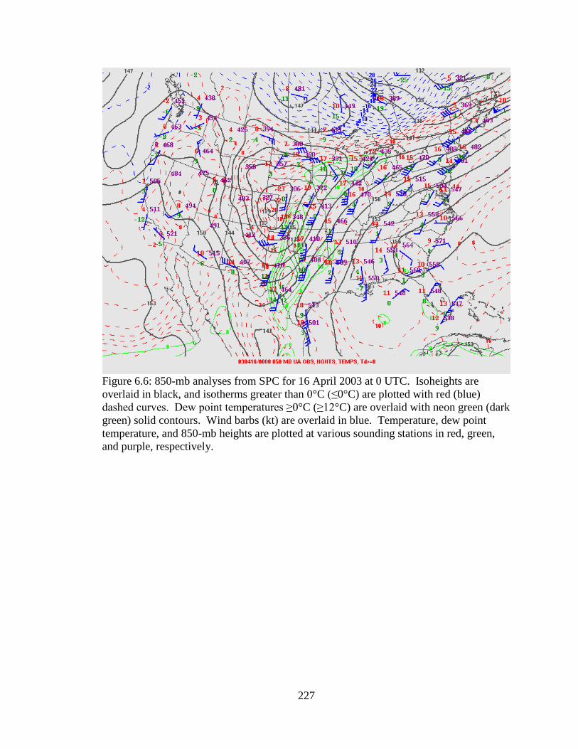
227

Figure 6.6: 850-mb analyses from SPC for 16 April 2003 at 0 UTC. Isoheights are

overlaid in black, and isotherms greater than 0°C (≤0°C) are plotted with red (blue)

dashed curves. Dew point temperatures ≥0°C (≥12°C) are overlaid with neon green (dark

green) solid contours. Wind barbs (kt) are overlaid in blue. Temperature, dew point

temperature, and 850-mb heights are plotted at various sounding stations in red, green,

and purple, respectively.

228

(a)

229

Figure 6.7: National Oceanic and Atmospheric Administration (NOAA) surface analyses

from (a) 15 April 2003 at 15 UTC and (b) 16 April 2003 at 3 UTC.

(b)

230

Figure 6.8: (a) Map showing the locations of upper air/METAR station Amarillo, TX

(KAMA) and METAR sites Childress, TX (KCDS), Abilene, TX (KABI), and Hobart,

OK (KHBR); (b) KAMA skew-T diagrams from 15 April 2003 at 12 UTC (green), 16

April 2003 at 00 UTC (blue), and interpolated to 15 April 2003 at 20 UTC (black) using

the observed 20 UTC surface temperature and dew point; (c) KAMA skew-T diagram

interpolated to 15 April 2003 at 22 UTC using the observed 22 UTC surface temperature

and dew point from KCDS. The orange curves in Figs. 6.8b-c denote surface lifted

parcel trajectories associated with the profiles plotted in black.

231

Figure 6.9: WSR-88D radar images of composite reflectivity over eastern New Mexico,

northern Texas, and Oklahoma at (a) 22 and (b) 23 UTC on 15 April 2003 and (c) 00, (d)

01, (e) 02, and (f) 03 UTC on 16 April 2003. Yellow arrows point to individual

supercells that are tornadic near the time of the image.

(a) (b)

(c) (d)

(e) (f)

232

Figure 6.10: (a) METAR site locations that reported dust, haze and/or reduced visibility

during 15-16 April 2003, (b) Dust, haze, and visibility METAR observations for 15-16

April 2003 as a function of time (hourly reports) and surface station (three letter

identifiers). Dust and haze reports are denoted by ‘D’ and ‘H’, respectively. Visibility is

represented numerically with units of statute miles. Yellow highlighting denotes a report

of visibility < 10 statute miles and/or a direct report of dust. Orange (red) denotes

visibility ≤ 5 (≤ 1) statute miles. ‘M’ indicates missing data.

(a)

(b)

233

Figure 6.11: Images of a major dust plume centered over the southwestern U.S. and the

Chihuahuan Desert region of Mexico on 15 April 2003 at 2020 UTC: (a) MODIS visible

composite, (b) application of a sophisticated dust detection algorithm supplied by Steven

Miller of CIRA, and (c) application of the “split window” technique.

(a) (b)

(c)

234

Figure 6.12: GOES-10 visible (albedo) imagery overlaid with “Split window” brightness

temperature differences (Tb,12.0 µm- Tb,10.7 µm) for (a) 1730, (b) 1930, (c) 2130, and (d)

2330 UTC.

235

CHAPTER 7

15-16 April 2003 Case Study

7.1 Model Setup

7.1.1 Model Configuration

The simulations presented in this chapter were performed using RAMS version

4.3 (Pielke et al. 1992; Cotton et al. 2003) in a polar stereographic horizontal coordinate

domain. Four two-way interactive nested model grids (Clark and Farley 1984) with

horizontal grid spacing of 30, 6, 2, and 0.5 km were employed (Fig. 7.1). The two outer-

most grids (Grid 1-2) were used for setting up the synoptic-scale flow as well as lofting

and handling the advection of dust. Grid 3 was employed to initiate and organize

convection. Grid 4 was used to assess individual supercell storms. Grids 1 and 2 were

initiated on 15 April 2003 at 06 UTC. Grid 3 was initiated at 20 UTC. Grid 4 was

initiated on 16 April at 0030 UTC. Simulations were run for 24 hours (completed on 16

April at 06 UTC). Soil moisture was initialized using ~30-km North American Regional

Reanalysis (NARR) data. The model was initialized with 1o×1

o data from the Global

Forecast System (GFS) model, as this dataset provided for more accurate surface winds

than produced by NARR and other model-based datasets.

The basic radiative condition (Klemp and Wilhelmson 1978a) was applied to the

normal velocity components at the lateral boundaries of Grid 1. The Mellor and Yamada

(1974) level 2.5 ensemble-averaged TKE scheme was utilized on Grids 1-3, while Grid 4

made use of the Smagorinsky (1963) deformation-K closure scheme with stability

modifications by Lilly (1962) and Hill (1974). Grids 1, 2, 3, and 4 had time steps of 30,

236

6, 2, and 0.5 s, respectively. Each grid had 39 vertical levels spanning ~20 km; spacing

increased from 50 m near the ground to a maximum of 1 km.

The surface processes were parameterized using LEAF-2 (Walko et al. 2000).

Radiation was parameterized using Harrington’s (1997) scheme. Convection was

parameterized on Grid 1 using the Kain-Fritsch (Kain and Fritsch 1990) cumulus

parameterization scheme and explicitly resolved on Grids 2-4. The dust source and

transport module utilized in these simulations was based on that of Ginoux et al. (2001),

modified by Smith (2007).

A bin-emulating, two-moment bulk microphysics scheme (Meyers et al. 1997;

Feingold et al. 1998; Saleeby and Cotton 2004, 2008) was utilized in these simulations.

The scheme explicitly predicted mixing ratios and number concentrations of pristine ice,

snow, aggregates, graupel, hail, cloud1 and cloud2 droplets, and rain. Nucleation by

CCN, GCCN, and IN was explicitly considered (Saleeby and Cotton 2004).

Heterogeneous ice nucleation was parameterized using the IN-based scheme of DeMott

et al. (2010). Homogeneous ice nucleation of cloud1, cloud2, and haze droplets was

parameterized using the DeMott et al. (1994) scheme. The model configuration used for

the simulations is summarized in Table 7.1.

7.1.2 Treatment of WRF/Chem CCN

The WRF/Chem-RAMS aerosol coupling scheme developed by Dan Ward

(section 3.3) was modified for more effective use in this study. First, the 15-16 April

2003 case study was simulated with WRF/Chem by Dan Ward using a single grid with

15-km horizontal grid spacing. However, previous sensitivity tests indicated that

237

WRF/Chem tends to over predict the κ parameter by roughly 60% (Dan Ward, personal

communication). Therefore, all values of κ produced by WRF/Chem in the 15-16 April

simulation were reduced by 60%. Second, WRF/Chem significantly overproduces CCN

number concentrations (in excess of 20,000 cm-3

). As such, the WRF/Chem output was

tuned to more realistic values using PM2.5 observations collected at –105.56o longitude,

40.36o latitude in eastern Rocky Mountain National Park during Spring of 2006 (Levin et

al. 2009). Model output from the nearest WRF/Chem grid cell at the lowest model level

was compared to the RMNP data. Average values of WRF/Chem CCN number

concentration and median radius were calculated for the simulated time period between

15 April at 0600 UTC and 15 April at 0600 UTC, and then compared to the mean values

reported by Levin et al. (880 cm-3

and 0.04 µm, respectively). The accumulation mode

size in WRF/Chem was underestimated by 50%, based on these comparisons. Noting

that the accumulation mode aerosol concentrations produced in WRF/Chem were

represented by a lognormal size distribution, this 50% underestimation in median radius

corresponded to a 70% overestimation of number concentration (assuming the

conservation of accumulation mode mass produced by the model). As a result, the

median radius dataset from WRF/Chem was multiplied by a size correction factor of 1.5,

while number concentrations were multiplied by a correction factor of 0.3. Clearly, there

are limitations to tuning the values within a regional dataset based on comparisons made

at a single location. However, this method provided a simple way for initializing the

RAMs simulations with realistic, horizontally heterogeneous background accumulation

mode aerosol based on output from the WRF/Chem model.

238

The original WRF/Chem-RAMS coupling scheme developed by Dan Ward

required that WRF/Chem output be created with the same number of nested grids at the

same horizontal grid spacing as the RAMS model setup. Then the aerosol data produced

in WRF/Chem would be ingested into RAMS and time-interpolated at some user-

specified time interval with a chosen model nudge factor. However, WRF/Chem output

was created for the 15-16 April 2003 case study using only a single grid at 15-km

horizontal spacing, far coarser than that of the inner-most RAMS grid (500 m).

Therefore, the WRF/Chem 15-km data were interpolated to RAMS Grids 1-3 at 5-min

intervals from model initialization on 15 April at 0600 UTC until 1200 UTC, when

aerosol concentrations reached their diurnal maximum. After 1200 UTC, aerosol

nudging with WRF/Chem was shut off so that CCN number concentrations were allowed

to freely advect and diffuse through the RAMS model domain. Allowing all of the

aerosol parameters (number concentration, median radius, mass, and κ) to be advected by

the model introduced artificial errors, where the mass and associated number

concentration, radius, and κ fields would lose consistency with each other in time.

Therefore, the median radius and κ of the background accumulation mode aerosol

distributions were held constant throughout the simulations for simplicity and

consistency. Mean values of adjusted WRF/Chem-based median radius and κ parameter

were calculated in the convective region of interest between 0600 UTC 15 April and

0600 UTC on 16 April. The background median radius was held constant at 0.035 µm,

while the background value of κ was set to 0.2 based on these calculations. Mass was

continually recalculated using a constant particle density of 1.8 g cm-3

. The final near-

239

surface CCN field that was simulated in RAMS on Grid 2 is shown in Figure 7.2 between

1200 and 2100 UTC on 15 April.

7.1.3 Experiment Design

In order to simulate the impacts of southwestern U.S. desert dust on convective

development and storm evolution during the 15-16 April severe storms outbreak, the

background CCN in RAMS was initiated with accumulation mode aerosol data adapted

from corresponding WRF/Chem output. However, WRF/Chem failed to produce any

coarse mode aerosol (simulated concentrations on the order of 10-19

cm-3

). Therefore, the

RAMS simulations were initialized with an idealized, horizontally homogeneous profile

of GCCN (Fig. 7.3). Three sensitivity simulations were performed. In one simulation,

neither dust microphysical nor radiative effects were included. This simulation will be

referred to as the control case (CTL). In another simulation, dust radiative effects were

included. However, dust concentrations were not allowed to serve as CCN, GCCN, or

IN. This will be referred to as the dust radiative impacts case (RAD). In the final

simulation, both dust radiative and indirect microphysical effects (dust allowed to serve

as CCN, GCCN, and IN) were included. This simulation will be referred to as the full

dust experiment (DST). The defining characteristics of each simulation are summarized

in Table 7.2.

7.2 Dust Scheme Validation

As discussed in Chapter 3 (section 3.2), the dust fine and coarse mode median

radii had to be set as constants for the case simulations. It was desirable to use AErosol

240

RObotic NETwork (AERONET) observations to set these constants. However, the only

AERONET site situated near the lofted dust plume that collected observations during the

event was located in Sevilleta, NM (–106.885o, 34.35

o). While the core of the dust plume

did not pass directly over this location during the 15-16 April dust event, median radii for

the fine and coarse mode aerosol distributions at this location still reached maximum

values around 2200 UTC on 15 April, then dropped off until 17 April (not shown). This

suggests that lofted dust likely impacted the measurements. Therefore, the fine mode

dust median radius in RAMS was set to 0.2 µm, and the coarse mode dust median radius

was set to 3.0 µm, based on values derived at Sevilleta on 15 April 2003 at 2200 UTC.

The METAR observations discussed in Chapter 6 (section 6.3) indicated that the

main source of lofted dust within the southwestern U.S. during 15-16 April 2003 was the

Chihuahuan Desert and possibly an agricultural based source in the Texas panhandle.

Therefore, the gridded dust source function used for these simulations was limited to the

Chihuahuan Desert region and crop sources in western Texas and eastern New Mexico.

The values of the source function in these regions were set to best replicate observed total

near-surface mass loadings throughout the duration of the dust event. Sensitivity

simulations were conducted on Grids 1 and 2. PM2.5 concentration measurements from

15-16 April 2003 were available at four Texas locations: El Paso (ELP), Amarillo

(AMA), Lubbock (LUB), and Odessa (ODE). PM10 concentrations were not available.

RAMS nearest-grid cell total dust mass concentrations (summation of the fine and coarse

modes) on Grid 2 were compared to the available PM2.5 concentrations at all four

locations, and the final dust source function was set in order to yield simulated near-

surface dust mass loadings that best matched corresponding PM2.5 concentrations. A map

241

of the tuned dust source function values used in the case simulations is displayed in

Figure 7.4. The Chihuahuan Desert region contained a maximum value of 0.11, while

values in the crop-based region in western Texas were set to 0.03 (Fig. 7.4). It should be

noted that by forcing the total RAMS near-surface dust mass loadings to match well with

observed PM2.5 loadings, the fine mode dust number concentrations produced in RAMS

might have been under-predicted compared to reality. This is because dust particles

larger than 2.5 µm contributed to the total dust mass in RAMS, as the coarse mode dust

median radius was set to 3.0 µm.

Figure 7.5 displays time series of observed surface PM2.5 and associated RAMS

nearest-grid cell dust mass concentrations on Grid 2 at ELP, AMA, LUB, and ODE from

1200 UTC on 15 April to 0600 UTC on 16 April during the DST simulation. PM2.5

concentrations at El Paso reached maximum values at 1800 UTC, while simulated dust

mass concentrations did not reach maximum values until 2200 UTC. PM2.5

concentrations at Lubbock reached their maximum values around 0000 UTC, while

simulated dust mass concentrations reached maximum values an hour later. However,

simulated mass concentrations approached roughly the same values as those observed.

Maximum simulated mass concentrations were delayed by 2 hours at Odessa (0000 and

0200 UTC, respectively). In addition, the observed maximum PM2.5 concentrations were

near 340 µg m-3

, while maximum simulated mass concentrations were only 240 µg m-3

.

Observed mass concentrations at Amarillo remained near zero throughout the dust event.

Simulated mass concentrations also remained low compared to the other locations.

However, these simulated concentrations reached 60 µg m-3

at 1400 UTC on 15 April,

remaining greater than 10 µg m-3

until 0300 UTC on 16 April. Furthermore, observed

242

mass concentrations dropped off quickly once maximum values were reached. Simulated

concentrations dropped off with time but at a much slower rate. It is clear that

discrepancies existed between the model and the observations with respect to the timing

of peak dust lofting at particular locations as well as dust atmospheric residence times.

Still, RAMS was able to replicate the maximum dust lofting over El Paso and Lubbock.

Simulated near-surface winds on Grid 2 at El Paso and Lubbock were compared

to observations to assess the timing discrepancies between the simulated lofted dust mass

loadings and the PM2.5 observations. These time series are presented in Figure 7.6.

Near-surface wind directions were simulated relatively well (often within 30o of reality)

at both El Paso and Lubbock (Fig. 7a-b). However, simulated wind directions at both

locations were off by more than 50o at 1500 UTC. The maximum surface wind speeds at

El Paso reached 22 m s-1

at 1900 UTC on 15 April. Simulated maximum wind speeds

were delayed by approximately 4 hours, with winds approaching 15 m s-1

(Fig. 7.6c).

Maximum observed wind speeds at Lubbock first reached 21 m s-1

at 2200 UTC.

Corresponding simulated winds reached only 16 m s-1

and were delayed by 3 hours (Fig.

7.6d). The DST simulation clearly produced weaker maximum winds over the dust

source regions of interest than observed, suggesting that the DST simulation would have

lofted less dust mass in the Chihuahuan Desert and west Texas crop region during the

event if given a source function based on actual winds. However, the maximum mass

loadings simulated by the DST experiment were tuned to corresponding observations at

these locations. This means that the fine and/or coarse mode dust median radius could

have been underestimated for these simulations, thus allowing particles to remain lofted

longer than in reality in order to compensate for reduced lofting at the source region.

243

Another possibility is that the dust mass loading in the Chihuahuan Desert region was

weaker in the simulations than in reality, and the simulated dust lofting from the

agricultural lands near Lubbock (which compensated for the under lofting in the

Chihuahuan Desert) was either overestimated or artificial. Nevertheless, the tuned dust

source function values (Fig. 7.4) allowed the simulations to achieve maximum dust mass

loadings close to reality in the convective region of interest (near Lubbock) during the

time of convection. Figure 7.7 displays column-integrated dust mass on Grid 2 from the

DST simulation at various times. It is plausible that simulated dust lofting was over-

predicted within the Texas panhandle. But overall, the advection of the dust plume

corresponded well with the observations presented in Chapter 6 (Fig. 6.12).

Note that the simulated maximum near-surface wind speeds were achieved

between 3 and 4 hours after the observations, consistent with the delayed dust mass

loadings evident in Fig. 7.5. The dust median radii used in this study were also likely set

too small based on the relatively slow mass dissipation rates simulated near the surface

compared to observations (Fig. 7.5). However, the degree of inaccuracy is difficult to

determine without more detailed observations of the aerosol size distribution associated

with the dust plume.

7.3 Simulation Results

7.3.1 Storm Evolution

Figure 7.8 displays VIC on Grid 2 for the DST, RAD, and CTL simulations

between 2230 UTC on 15 April and 0300 UTC on 16 April. Convection initiated in each

simulation just before 2230 UTC (not shown) within the Texas panhandle. At 2230

244

UTC, two distinct convective cells began developing in the eastern portion of the

panhandle (Fig. 7.8a-c). By 0000 UTC on 16 April, a convective line had formed in the

DST case. The line extended from Kansas southward through Oklahoma into central

Texas. Mature convective cells were embedded within the northern portion of the line,

seen as multiple convective cells associated with VIC values greater than 10 mm located

at the border of Texas and Oklahoma. Convective cell growth within the line built

toward the southwest, as younger, weaker cells developed in central Texas (Fig. 7.8d).

The development of the convective line in the RAD and CTL cases resembled that of the

DST simulation. However, the RAD and CTL convective lines were associated with

fewer discrete convective cores at this time (Fig. 7.8e-f). At 0130 UTC, all three

convective lines contained multiple embedded convective elements with maximum VIC

values greater than 10 mm, extending from southern Kansas into central Texas (Fig. 7.8g-

i). However, the largest cells associated with VIC greater than 10 mm were located at the

northern end of the DST convective line, while such cells in the RAD and CTL cases

were located toward the southern portion of the line. The line continued its movement

toward the east. By 0300 UTC, the northern most cells had merged into larger

convective systems, defined by large regions of VIC values greater than 10 mm in central

Oklahoma in all three simulations (Fig. 7.8j-l). Spatially smaller storms were located

further south in Texas. The DST convective line now resembled a leading stratiform-like

system, as a large region of VIC greater than 1 mm was located immediately east of the

convection. This feature was less evident in the RAD and CTL cases.

Overall, the convective line evolved in a similar manner among the three

simulations on Grid 2 with respect to the timing and location of convection. However,

245

spatial variations in VIC between all three cases suggested that dust influences played a

role in the evolution of the convective line. In particular, convection at the southern-most

tip of the convective line at 0300 UTC was associated with notably lower values of VIC

in the CTL case compared to the DST and RAD simulations (Fig. 7.8j-l). Further

analyses focused on the southern half of the simulated convective line, as it was the tail

end of the line that spawned supercell-like storms in the simulations.

The time evolution of the total condensate field at 1 km on Grid 4 is shown in

Figure 7.9 for all simulations. Updrafts are overlaid at 10 and 20 m s-1

. Convection was

triggered on Grid 3 around 0030 UTC in the DST simulation. This convection organized

and began exhibiting classic supercell-like characteristics by 0100 UTC (not shown).

The developing storm moved into Grid 4 at 0110 UTC and began splitting into two cells

by 0120 UTC (not shown). By 0130 UTC, two distinct cells were moving through the

northwestern portion of Grid 4 (Fig. 7.9a). The left mover propagated off of the grid over

the next 20 minutes and was not considered further. The right-moving supercell moved

eastward through the northern half of Grid 4. This cell was characterized by a core

updraft, a distinct hook in the total condensate field associated with the RFD

precipitation, and a region of total condensate greater than 0.5 g kg-1

(peak values greater

than 4 g kg-1

) located north and northeast of the main updraft, corresponding to

precipitation within the FFD (Fig. 7.9a,d). The RAD and CTL cases failed to produce

isolated cells at this time (Fig. 7.9a-c). Instead, a continuous convective line oriented

southwest-to-northeast was propagating through Grid 4, associated with extensive regions

of total condensate values greater than 4 g kg-1

. The northern portion of the convective

line possessed an updraft with maximum vertical velocities greater than 10 m s-1

in both

246

simulations (Fig. 7.9b-c). The southern portion of the convection in the CTL case was

also characterized by a small updraft region at its leading end (Fig. 7.9c).

A second supercell storm moved into the southwestern corner of Grid 4 in the

DST simulation at 0200 UTC (Fig. 7.9d), exhibiting similar characteristics as the cell

further north, including a main updraft with maximum vertical velocities at 3.5 km

greater than 20 m s-1

, an RFD hook signature in the total condensate field, and a broad

region of total condensate greater than 0.5 g kg-1

within the FFD north of the main

updraft. Another small region of total condensate values greater than 4 g kg-1

corresponded to the precipitation core within the FFD. The convection in the RAD

simulation had organized into two distinct cells by this time (Fig. 7.9e), both showing

signs of supercell activity. This included main updrafts, total condensate greater than 4 g

kg-1

within the FFD, and slight cyclonically-curved hooks in the total condensate field

greater than 0.5 g kg-1

located toward the rear of the storms associated with the RFD.

The convective line in the CTL case was weakening at this time (Fig. 7.9f), suggested by

the dissipation of updraft cores and a reduction in areal coverage of regions of the total

condensate field greater than 4 g kg-1

. Additional storm weakening was evident 30

minutes later (Fig. 7.9i). On the contrary, the northern supercell in the DST simulation

split again on Grid 4 between 0210 and 0220 UTC (not shown). At 0230 UTC, the right-

moving supercells continued to move in a westerly-southwesterly direction, while the

left-moving storm in the northern portion of the grid moved to the northeast (Fig. 7.9g).

The hook signatures associated with the RFD in the two right-moving cells were less

distinct at this time. The southernmost storm in the RAD simulation continued to

organize and move in a westerly direction (Fig. 7.9h). However, the cell that showed

247

signs of supercell growth at 0200 UTC in the northern portion of the grid had dissipated

by 0230 UTC. By 0300 UTC, the northern cells in the DST simulation were exiting Grid

4, while the southern supercell continued to move eastward across the grid (Fig. 7.9j).

The RAD supercell continued to move through the southern portion of Grid 4 at 0300

UTC, characterized by a FFD with maximum total condensate values greater than 4 g kg-

1 covering a broad region and weaker values associated with the RFD. New convection

developed to the southwest (Fig. 7.9k). The unorganized, scattered convective line

simulated in the CTL case at 0300 UTC continued to weaken as it propagated out of Grid

4 (Fig. 7.9l). No updraft cores with velocities greater than 10 m s-1

existed by this time.

7.3.2 Dynamics on Grid 4

The DST simulation produced two distinct supercell-like storms on Grid 4, while

the RAD and CTL simulations produced more widespread convection and heavier

precipitation. However, Grid 4 convection in all three simulations was associated with

two distinct storm tracks: one in the northern portion of the grid and the other further

south. Therefore, Grid 4 was divided into a northern sub region (North-Region 1, or

NR1) and a southern sub region (South-Region 2, or SR2) for better analysis of each

storm. The western boundary of Grid 4 was separated at latitude 32.6o, while the eastern

boundary was separated at latitude 32.8o. This delineation latitude varied linearly

between the east and west boundaries. Figure 7.10 displays the time evolution of

maximum vertical relative vorticity between 2 and 6 km on Grid 4 for all simulations

from 0130 UTC to 0330 UTC in 30-min intervals. The boundary of the NR1 and SR2

regions is plotted in each figure panel as a dashed line. Vorticity was contoured at 0.02

248

and 0.05 s-1

. Each simulation formed supercell storms. Two distinct centers of vertical

vorticity were evident in the DST simulation (Fig. 7.10a). The NR1 supercell exhibited

maximum mid-level vorticity values greater than 0.05 s-1

at 0200 UTC, then values

slowly weakened with time. The SR2 supercell was associated with maximum values of

vorticity greater than 0.02 s-1

throughout its life cycle. Both supercells were

characterized by distinct vorticity maxima for four of the plotted time periods. The RAD

simulation also produced two different centers of vertical vorticity, with one center

propagating through the NR1 region and the other through the SR2 region. However,

only the SR2 cell organized into a long-lived supercell that possessed mid-level vertical

vorticity with maximum values greater than 0.02 s-1

for four time periods (Fig. 7.10b).

The NR1 vorticity maximum possessed noticeably smaller areal coverage and only

existed between 0130 and 0200 UTC. The convective line produced in the CTL

simulation also failed to produce a strong, long-lived supercell storm. A small vorticity

center was produced in the NR1 region at the same time periods as the RAD simulation.

The SR2 sub region failed to produce vertical vorticity greater than 0.2 s-1

during the

displayed time periods (Fig. 7.10c). The CTL SR2 sub region did produce a weak

supercellular storm between 0140 and 0230 UTC. However, the storm was associated

with maximum values of vertical vorticity of only 0.033 s-1

at 0210 UTC.

Maximum vertical vorticity was often achieved at times not displayed in Fig.

7.10. Furthermore, maximum values often developed in the lowest 2 km of the more

explosive, longer-lived supercells that were produced by the DST and RAD simulations.

Table 7.3 summarizes the defining characteristics of all six simulated supercells, based on

the location of maximum relative vertical vorticity below 6 km in each sub region of Grid

249

4 between 0030 and 0400 UTC for each simulation. Table values are based on the

surrounding 10×10 km region of each vorticity center. The strongest, longest-lived

supercell was produced by the DST simulation within the NR1 region. This supercell

was associated with the greatest maximum updrafts, surface winds, surface pressure

deficits, surface convergence, and relative vertical vorticity below 6 km (Table 7.3). The

DST and RAD simulations created comparable supercells in the SR2 region. The DST

supercell yielded greater maximum updrafts and surface winds, surface convergence, and

vertical vorticity below 6 km. The RAD supercell obtained a slightly greater surface

pressure deficit within the near-vortex region and greater storm-relative surface winds.

The supercells that developed in the CTL simulation as well as that in the NR1 region

during the RAD case were shorter-lived, weaker storms than the others. However, the

supercell produced by the CTL simulation in the NR1 region was associated with the

second highest maximum vertical vorticity value (0.08 s-1

at 0150 UTC; the DST NR1

supercell possessed maximum vertical vorticity of 0.14 s-1

at 0200 UTC), even though

values quickly faded by 0200 UTC and were no longer present by 0220 UTC. The RAD

NR1 supercell failed to develop large vertical vorticity over any extended period of time.

Maximum values reached 0.053 s-1

at 0220 UTC.

Figure 7.11 displays profiles of peak and mean updrafts and downdrafts in the

NR1 sub region of Grid 4 for each simulation at 0140 and 0230 UTC on 16 April, as

these time periods generally represent the updraft structures observed throughout the

simulations while supercell storms were present. At 0140 UTC, the supercell in the DST

simulation produced the strongest peak updrafts below 5 km, with maximum peak

updrafts approaching 60 m s-1

just above 1 km (Fig. 7.11a), associated with a strong low-

250

level mesocyclone at this time. The RAD simulation produced the weakest peak

updrafts, with maximum values less than 40 m s-1

between 5 and 12 km. Similar

differences among the simulations are evident in the mean updraft profiles (Fig. 7.11b).

The CTL simulation yielded the greatest mean updrafts overall. In contrast, the RAD

simulation produced the strongest peak downdrafts in the lowest 5 km at this time (Fig.

7.11c), with peak downdrafts exceeding 23 m s-1

near 2.5 km and roughly 13 m s-1

just

below 1 km. The RAD simulation yielded the strongest mean downdrafts near the

surface, while the DST simulation was associated with the weakest downdrafts on

average below 2 km (Fig. 7.11d). By 0230 UTC, the DST simulation produced the

strongest peak updrafts at all levels (Fig. 7.11e), with maximum values exceeding 40 m s-

1 at 7 km. The RAD and CTL simulation produced comparable peak updrafts. The CTL

simulation created the greatest updrafts between 3 and 8 km on average (Fig. 7.11f). The

DST simulation was associated with the strongest peak and mean downdrafts at low

levels at this time (Fig. 7.11g-h), with maximum peak and mean downdrafts reaching 14

and 1.7 m s-1

, respectively. Similar results were found amongst the simulations at 0200

and 0230 UTC in the SR2 region (Fig. 7.12). The supercells produced in the DST

simulation yielded the greatest peak updrafts and initially, possessed relatively weak low-

level downdrafts. With time, however, the DST supercells went on to produce stronger

downdrafts at low levels compared to the RAD and CTL simulations.

7.3.3 Precipitation and Cold-Pool Evolution

Grid 4 precipitation rates are shown in Figure 7.13 for each simulation at 30-min

intervals. At 0130 UTC, the NR1 right-moving supercell in the DST simulation is

251

located in the northwestern portion of Grid 4 splitting off from its left-moving

counterpart (Fig. 7.13a). The right-mover exhibits a classical supercell structure in the

precipitation field, with a hook pattern affiliated with the RFD precipitation wrapping

around the main updraft and considerable precipitation rates within the FFD. Maximum

rates exceed 125 mm h-1

. The left-moving storm is characterized by a single core of

precipitation rates greater than 200 mm h-1

. The convective lines in the RAD and CTL

simulations at this time are defined by two elongated precipitation cores of considerable

horizontal extent, possessing precipitation rates greater than 200 mm h-1

(Fig. 7.13b-c).

At 0200 UTC, maximum precipitation rates are located near the RFD for both supercells

produced by the DST simulation (Fig. 7.13d). The NR1 cell is affiliated with a small

region of precipitation rates greater than 200 mm h-1

, while the SR2 cell contains a small

region with rates greater than 125 mm h-1

. The two storms in the RAD case are

dominated by precipitation rates exceeding 200 mm h-1

(Fig. 7.13e). In the CTL case for

the same time period, the convection in the NR1 sub region is broken up into three cores

of precipitation rates exceeding 200 mm h-1

, while the southern end of the line (located in

SR2) shows two small precipitation cores with maximum rates greater than 75 and 100

mm h-1

, respectively (Fig. 7.13f). Thirty minutes later the precipitation rate pattern

associated with the DST supercells contains a well-defined hook near the RFD, defined

by relatively weak precipitation rates and heavy precipitation rates within the FFD (Fig.

7.13g). The NR1 and SR2 cells show maximum precipitation rates greater than 150 and

125 mm h-1

, respectively. The storms in the RAD simulation have both weakened

substantially by 0230 UTC (Fig. 7.13h). However, the SR2 cell still possesses a

precipitation core with precipitation rates exceeding 150 mm h-1

within the FFD.

252

Convection in the SR2 region of the CTL case has strengthened at this time (compared to

30 min prior), while precipitation in the NR1 region has weakened. Both sub regions

show small cores of precipitation rates just greater than 150 mm h-1

at this time (Fig.

7.13i). By 0300 UTC, the NR1 supercell in the DST simulation is still characterized by a

well-defined RFD and weak precipitation rates. Precipitation rates have weakened

notably within the FFD. The SR2 supercell is associated with a small core of

precipitation rates greater than 150 mm h-1

that is now located near the RFD (Fig. 7.13j).

Precipitation rates in the RAD simulation at this time show small, scattered convective

cores with rates greater than 150 mm h-1

(Fig. 7.13k). Overall, precipitation rates have

been greatly reduced in the CTL simulation (Fig. 7.13l). By 0330 UTC, only the SR2

supercell remains in the DST simulation (Fig. 7.13m). The SR2 supercell in the RAD

simulation continues to precipitate out while new convective precipitation develops

further to the southwest (Fig. 7.13n). This pattern is evident in the CTL case as well.

However, convection is weak, and precipitation rates are rather low. Only a single core

defined by precipitation rates greater than 10 mm h-1

persists near the center of Grid 4

(Fig. 7.13o).

Grid 3 and Grid 4 accumulated precipitation is displayed in Figure 7.14. Both

grids were displayed in order to show that the field on Grid 4 for each simulation was

overall similar to its respective larger view on Grid 3. Therefore, analysis focused on the

inner most grid results (Fig. 7.14d-f), as storm microphysics were better represented at

the horizontal grid spacing of Grid 4 (500 m). The accumulated precipitation pattern

produced by every simulation showed why the grid was broken up into the NR1 and SR2

sub regions, as two main storm tracks were evident. The RAD and CTL simulations

253

clearly produced more accumulated precipitation on Grid 4 than the DST case. The

precipitation signature within the NR1 region of the DST simulation revealed two distinct

storm splits, where both left-moving systems exited the northern boundary of the grid

(Fig. 7.14d). The right-mover moved across the northern half of grid 4, and produced a

maximum accumulated precipitation amount just greater than 45 mm in the northeastern

quadrant of the grid. The SR2 supercell was generally associated with weaker

precipitation rates compared to the NR1 storm, and therefore yielded reduced

accumulated precipitation along its track. Maximum values were generally below 35

mm. The RAD simulation resulted in notably more accumulated precipitation along each

storm track (Fig. 7.14e). Storm-splitting was evident in both the northwestern portion of

the NR1 track as well as in the southwestern region of the SR2 track. Both tracks were

associated with elongated regions of accumulated precipitation amounts exceeding 65

mm, with the SR2 track yielding such high accumulation totals throughout most of its

length. A third storm track was located near the southern boundary of the grid (within

the SR2 sub region), due to the continued development of convection southwest of the

main SR2 supercell. Totals along this track never exceeded 25 mm. A similar pattern

was evident in the CTL simulation (Fig. 7.14f). However, the CTL NR1 storm track was

associated with the most accumulated precipitation, with a large region of values greater

than 65 mm located in the western half of Grid 4. The SR2 storm track was associated

with less accumulation, as maximum amounts failed to reach 50 mm. Much of the SR2

storm track was associated with maximum accumulated amounts below 35 mm.

Grid-cumulative accumulated precipitation and maximum precipitation rates were

calculated for the NR1 and SR2 regions on Grid 4 for each simulation (Fig. 7.15).

254

Convection in the NR1 region for the CTL simulation (red solid curves) produced the

greatest precipitation rates until 0115 UTC (Fig. 7.15b) and thus produced the highest

accumulation totals of any sub grid in any simulation (Fig. 15a). The CTL SR2 region

was associated with weaker precipitation rates and thus reduced accumulated

precipitation (red dashed curves). Recall that the supercells spawned in this simulation

were generally weak and short-lived compared to those produced by the DST simulation.

The NR1 sub region of Grid 4 in the RAD simulation produced the second highest total

accumulated precipitation (Fig. 7.15a, blue solid curve) through 0345 UTC and the

heaviest precipitation rates overall, with maximum values approaching 700 mm h-1

(Fig.

7.15b, blue solid curve). Again, no long-lived supercells were produced in this region.

The SR2 region in the RAD simulation yielded the second highest maximum

precipitation rates (Fig. 7.15b, blue dashed curve) and the second highest accumulated

precipitation amounts overall (Fig. 7.15a, blue dashed curve), because convection

continued to develop to the southwest of existing cells on Grid 4. Thus, accumulated

precipitation in the SR2 region became greater than that of NR1 after 0345 UTC. Recall

that the RAD simulation produced a long-lived supercell storm in the SR2 sub region.

The DST simulation created long-lived supercell storms in both sub domains of Grid 4.

The NR1 (black solid) and SR2 (black dashed) regions yielded the second lowest and

lowest accumulated precipitation amounts, respectively (Fig. 15a). They also possessed

the weakest maximum precipitation rates (Fig. 7.15b). However, the SR2 region was

associated with precipitation rates greater than many of the other Grid 4 sub domains

after 0300 UTC, as a supercell storm continued to move through the southern portion of

the grid in the DST simulation at this time.

255

Grid 4-cumulative precipitation accumulation and maximum precipitation rates

were also calculated (Fig. 7.16). Overall, the DST simulation yielded less than half of the

total accumulated precipitation as the RAD and CTL (Fig. 7.16a). The DST simulation

was consistently associated with weaker precipitation rates than those in the RAD and

CTL cases (Fig. 7.16b). In general, the longer-lived supercells generated by the DST and

RAD simulations were associated with weaker precipitation rates and lower accumulated

precipitation amounts than the sub domains of the RAD and CTL simulations that failed

to produce long-lived, organized convection. The CTL SR2 sub domain produced no

noteworthy precipitation overall, as heavy precipitation in the NR1 region prevented the

triggering of strong convection in the SR2 sub domain.

Figure 7.17 displays near-surface temperature on Grid 2 at 2200 UTC on 15 April

and at 0200 UTC on 16 April to show pre-convective surface temperatures as well as

non-convective surface temperatures after convection had been triggered. Convective

(and non-convective precipitation) regions are overlaid, represented by VIC greater than

0.01 mm. Pre-convective temperatures in the Texas panhandle reached values greater

than 26oC by 2200 UTC on 15 April (Fig. 7.17a-c), while values exceeded 30

oC in

southwestern Texas. However, by 0200 UTC on 16 April when convection had initiated

in the region, temperatures had cooled to values closer to 24oC behind the main

convective line in each simulation, due to radiative cooling after sunset as well as the

eastward propagation of the cold front that spanned the southern U.S. (Fig. 7.17d-f).

Surface temperatures were near 22oC east of the main line. Surface temperatures within

convective cold-pool regions reached lower values. Figure 7.18 displays surface

temperatures on Grid 4 for each simulation between 0200 and 0330 UTC on 16 April. At

256

0200 UTC the DST simulation yielded the weakest cold-pools, associated with two

mature supercells (Fig. 7.18a). Minimum surface temperatures were near 20oC, only 2

oC

colder than surface temperature east of the convective line. Temperatures behind the line

were closer to 24oC. The RAD simulation produced the strongest cold-pool in the NR1

region (Fig. 7.18b), with minimum surface temperatures reaching 17oC. The cold-pool in

the SR2 region was associated with temperatures as low as 19.5oC. A similar surface

pattern is seen in the CTL simulation at this time (Fig. 7.18c), with a large portion of the

NR1 region associated with temperatures less than 17oC and slightly weaker cold-pools

in the SR2 region. At 0230 UTC, the DST simulation was still characterized by two

distinct cold-pools associated with the two supercells moving through the grid (Fig.

7.18d), while temperatures colder than 21oC existed throughout much of the grid in the

RAD and CTL simulations (Fig. 7.18e-f), associated more widespread convection with

heavy precipitation (and embedded weak supercells). By 0300 UTC, the NR1 supercell

in the DST simulation had produced a cold-pool at the surface with a small region of

temperatures just below 21oC, while the left-mover was associated with noticeably colder

temperatures to the northwest. The second DST supercell in the SR2 region was

associated with a small region of temperatures colder than 19oC, associated with

precipitation within the storm’s FFD (Fig. 7.18g). The RAD and CTL simulations were

still characterized by widespread cold-pools at this time (Fig. 7.18h-i), and the RAD

supercell in the SR2 region was producing the strongest cold-pool among the simulations.

Minimum surface temperatures in the CTL case were slightly warmer than 30 min prior,

as precipitation had weakened. At 0330 UTC, the cold-pool affiliated with the DST SR2

supercell (Fig. 7.18j) was colder than that in the RAD simulation (Fig. 7.18k). The CTL

257

simulation produced the strongest cold-pool at this time due to the presence of some

short-lived, non-supercell convection (Fig. 7.18l).

The horizontal coverage of cold-pools produced in the DST simulation was lower

than that of the other cases, because the CTL and RAD simulations produced more

widespread heavily-precipitating convection within the main line, while the DST

simulation produced more isolated supercells associated with weaker precipitation rates.

However, note that the supercells in the DST simulation yielded colder cold-pools than

the RAD and CTL simulations at times, even though these supercells continuously were

associated with the weakest precipitation rates and lowest overall accumulated

precipitation.

7.3.4 Dust Microphysical Effects

The differences in precipitation and storm evolution between the DST simulation

and the RAD and CTL cases coincide with microphysical differences between the

simulations, due to the presence of dust serving as CCN, GCCN, and IN in the DST case.

7.3.4.1 Hydrometeor Size Spectra

Figure 7.19 displays mean profiles of cloud1 and cloud2 droplet mixing ratio,

number concentration, and median diameter within updrafts greater than 1 m s-1

on Grid 4

at 0200 UTC on 16 April in the NR1 region. Convection in the RAD and CTL

simulations produce nearly identical profiles of cloud1 mixing ratio and number

concentration (Fig. 7.19a-b). The DST simulation yields the smallest mixing ratios but

the highest number concentrations of cloud1 droplets. The cloud1 droplets in the DST

258

simulation are also of significantly smaller size on average than those in the RAD and

CTL simulations (Fig. 7.19c). Mean median diameters in the RAD and CTL simulations

approach 50 µm, while those in the DST simulations range between 10 and 30 µm.

Similarly, the RAD and CTL simulations yield nearly identical profiles of mean cloud2

mixing ratios (Fig. 7.19d), while mixing ratios in the DST simulation are roughly 50%

lower. The DST simulation also produces slightly lower number concentrations of

cloud2 droplets than the RAD and CTL simulation on average (Fig. 7.19e). The cloud2

droplets produced in the DST simulation are also smaller in size than those of the RAD

and CTL simulation (Fig. 7.19f). Median diameters in the DST simulation fall between

70 and 89 µm, while those in the RAD and CTL simulations are higher, ranging between

90 and 98 µm. Figure 7.20 displays the same profiles but for the SR2 region at 0210

UTC. More spread exists between the three simulations in this sub domain, as the CTL

simulation resulted in little SR2 convection. The CTL simulation produces the lowest

cloud1 mixing ratios, while the RAD simulation produces the largest (Fig. 7.20a). In

contrast, the CTL simulation produces the highest cloud2 mixing ratios (Fig. 7.20d), and

the DST simulation produces the lowest. Just as in the NR1 region, the highest number

concentrations of cloud1 droplets are found in the DST simulation (Fig. 7.20b), cloud2

droplet concentrations are comparable but slightly lower in the DST case compared to the

other simulations (Fig. 7.20e), and the DST simulation produces cloud1 and cloud2

droplets of notably smaller size (Fig. 7.20c,f).

The resulting raindrop, graupel, and hail stone size spectra differed among the

simulations. Mean profiles of rain, graupel, and hail number concentrations as well as

median diameter in updrafts and downdrafts in the NR1 region are plotted for each

259

simulation in Figure 7.21 at 0200 UTC. The DST simulation produced lower raindrop

concentrations than the RAD and CTL simulations within updraft regions (Fig. 7.21a),

while the highest concentrations were found in the CTL simulation (>7000 m-3

above 2

km). The DST simulation produced the largest raindrops above 2 km (Fig. 7.21b).

Within downdrafts, the DST simulation still produced the lowest number concentrations

of rain below 5 km but of comparable sizes to those in the RAD and CTL simulations

(Fig. 7.21d). The DST simulations yielded significantly higher graupel concentrations

within updrafts than the RAD and CTL simulations (Fig. 7.21e). Maximum mean

concentrations were roughly four times larger than in the RAD simulation (8000 vs. 2000

m-3

at 8 km, respectively). Concentrations in the RAD simulation were slightly higher

than those in the CTL case. However, the graupel produced in the DST simulation was

associated with mean median diameters between 0.6 and 0.7 mm, notably smaller than

those in the RAD (0.7 to 1.2 mm) and CTL (0.8 to 1.4 mm) simulations (Fig. 7.21f).

This was also the case within downdraft regions (Fig. 7.21g-h). The DST simulation

yielded significantly higher number concentrations of graupel but of smaller sizes than

those produced by the RAD and CTL simulation. The same comparisons were found

with respect to hail production. The DST simulation produced the highest hail number

concentrations within updrafts (Fig. 7.21i) and downdrafts (Fig. 7.21k) but of smaller

sizes than the RAD and CTL simulations (Fig. 7.21j,l). The RAD simulation produced

slightly higher concentrations of graupel and of larger sizes compared to the CTL case.

The same comparisons were found in the SR2 region at 0210 UTC (Fig. 7.22). However,

at this time, the DST supercell was associated with the largest raindrops in both updraft

260

(0.6 mm at 2 km) and downdraft (1 mm near the surface) regions below 3 km (Fig.

7.22b,d). Graupel production was greatly reduced in the CTL SR2 region.

7.3.4.2 Grid-Cumulative Hydrometeor Mass

Figure 7.23 shows time series of various NR1 and SR2 sub grid-cumulative

hydrometeor mass on Grid 4 for each simulation. The RAD simulation and the NR1

region of the CTL case produced the greatest amounts of cloud1 mass after 0140 UTC

(Fig. 7.23a). Between 0140 and 0300 UTC, the CTL SR2 sub domain produced the least

amount of cloud1 water. Both NR1 and SR2 regions in the DST simulation yielded the

least amount of cloud2 water mass (Fig. 7.23b). Cloud2 amounts in the RAD and CTL

NR1 regions were nearly identical, while the CTL SR2 region produced the most cloud2

water mass after 0130 UTC. The NR1 and SR2 regions of the DST simulation yielded

the least cumulative rain mass (Fig. 7.23c). The heavily-precipitating convective lines in

the NR1 regions of the RAD and CTL simulations produced the greatest cumulative rain

mass below 5 km until 0220 UTC (maximum values greater than 80,000 kg). After this

time, the supercell in the SR2 region of the RAD simulation was associated with the most

rain. However, the DST SR2 and NR1 regions yielded the highest and second highest net

small ice particle mass above 5 km, respectively (both greater than 60,000 kg). The RAD

supercell in the SR2 region produced the third highest totals, peaking at 0210 UTC (Fig.

7.23d). The RAD and CTL NR1 regions, which produced the greatest rainfall, yielded

even less small ice particle mass aloft. The DST NR1 supercell created the most graupel

mass (greater than 40,000 kg between 0100 and 0200 UTC), while the CTL NR1 region

yielded the second highest maximum amounts (Fig. 7.23e). The DST SR2 region yielded

261

the third highest totals. The RAD NR1 and SR2 sub domains produced comparable

graupel mass, while the CTL SR2 region accumulated the least sub grid-cumulative

graupel. The RAD and CTL NR1 regions accumulated the highest hail mass overall (Fig.

7.23f), with peak values greater than 100,000 kg at 0130 UTC. The DST NR1 and RAD

SR2 sub regions yielded similar maximum hail mass. The DST SR2 region was

associated with maximum values near 40,000 kg. The CTL SR2 region produced the

lowest accumulated hail mass (maximum values near 30,000 kg).

7.3.4.3 Cause and Effect

It is not possible to determine exactly how much dust served as CCN, GCCN, and

IN in the DST simulation (or how often) without more sophisticated microphysical

budgets installed in RAMS. However, various print statements throughout the simulation

indicated that the fine mode dust did not effectively serve as CCN in this study. Instead,

the presence of the dust actually reduced the overall ability of the total aerosol population

to nucleate cloud drops. Recall that the fine mode dust and background CCN were

combined into a bulk lognormal distribution just prior to nucleation, making use of the κ

parameter and the assumption of internally-mixed particles. In the DST simulation, the

number concentration of fine mode dust was significantly lower than that of the

background population, so the overall number of potential CCN was not increased by the

presence of dust. The dust was also of larger size but of significantly lower

hygroscopicity. This meant that the dust increased in the median size of the bulk fine

mode aerosol population; however, the bulk value of κ was lowered significatly from 0.2

to values much closer to 0.03. With such lower values of κ, cloud1 droplet nucleation

262

was greatly reduced in the DST simulation compared to the RAD and CTL simulations,

and cloud1 droplets in the DST simulation did not grow to the sizes found in the other

simulations. With cloud1 droplets 4-5× smaller in the DST case (Figs. 7.19-7.20),

autoconversion was greatly reduced, which yielded fewer cloud2 droplet concentrations,

and cloud2 droplets were of smaller size than those produced in the RAD and CTL

simulations (Figs. 7.19-7.20). Print statements during model runtime indicated that the

coarse mode dust also served as GCCN in the DST simulations, which nucleated

relatively large cloud2 droplets due to size of the coarse mode dust. However, with such

low number concentrations of cloud2 droplets produced in the DST simulation and the

cloud2 droplets produced in the DST simulation generally being 10 to 20 µm smaller

than those in the RAD and CTL cases, it is clear that the impact of the fine mode dust

reducing CCN activation played a far greater role on the resulting cloud2 droplet spectra

than of the coarse mode dust serving at times as GCCN. More sophisticated dust

microphysical budgets will have to be installed in RAMS or more idealized simulations

isolating the impacts of dust serving as CCN against dust serving as GCCN will have to

be performed in order to truly distinguish the two processes. In any case, with smaller

cloud droplets and reduced autoconversion, the warm rain process was severely reduced

in the DST simulation. However, due to the abundance of cloud drops available and

higher in-cloud trajectories and thus longer net liquid water paths, the raindrops that did

form were able to grow to larger sizes compared to the RAD and CTL simulations. This

is consistent with the simulation results presented in Chapter 5 as well as from other

RAMS simulations (e.g., Storer et al. 2010). Instead, the small cloud drops were sent

into the mixed-phase region of the updraft, which upon freezing, enhanced latent heating

263

and helped to strengthen peak updrafts within DST convective cells (Figs. 7.11-7.12).

With considerably more ice mass aloft in the DST simulations (Fig. 7.23d) and numerous

small cloud drops available for riming, the DST simulation produced the highest graupel

concentrations among the simulations but of relatively small size due to reduced riming

efficiencies and hence reduced riming rates of small cloud droplets. The RAD and CTL

simulations had notably less graupel embryos compared to the DST simulation.

However, with larger cloud drops available (and thus greater riming rates), the graupel

that did form in the RAD and CTL updrafts were of larger size than that of the DST case

(Figs. 7.21-7.22).

With such a high proficiency for creating small graupel, the DST simulation also

produced the largest hail number concentrations. However, the RAD and CTL

simulations yielded higher riming efficiencies and riming rates than the DST, due to the

presence of larger cloud droplets and higher number concentrations of supercooled

raindrops. As a result, the hail that was formed in the RAD and CTL cases grew to larger

sizes (Figs. 7.21-7.22). With severely reduced warm rain processes and reduced riming

rates, the DST simulation yielded convection with the lowest rainfall rates and

accumulated precipitation. However, the DST downdraft regions were associated with

higher number concentrations of smaller graupel and hail particles. As these particles fell

within downdrafts below the melting level, associated melting and evaporation of these

small hydrometeors resulted in enhanced cooling, increased negative buoyancy, and thus

at times, stronger downdrafts than those produced in the RAD and CTL simulations.

However, with significantly reduced rainfall overall, this effect was often not enough to

create stronger downdrafts than what was produced in the RAD and CTL simulations

264

where precipitation was greater (Figs. 7.11-7.12). Even though the DST simulation

produced such high number concentrations of graupel and hail, much of the total mass

was distributed into particles of small enough sizes to remain lofted in the storm and

eventually be ejected into the storm anvils rather than falling as precipitation. The

combined effects of warm rain efficiency, ice production, and hydrometeor size together

controlled the overall evolution of cold-pools and storm structure. The RAD and CTL

convective lines initially produced copious amounts of warm rain on Grid 4 between

0040 and 0200 UTC, while the DST simulation saw a reduction in warm rain production.

As a result, the RAD and CTL simulations produced widespread regions of heavy

precipitation, which yielded widespread cold-pool production of varying temperature.

This hindered the early formation of any long-lived, classical type supercells in these

simulations, even though supercells tried to spin up in both simulations after 0100 UTC.

The DST convective line was associated with reduced rainfall and thereby able to form

multiple discrete supercells that produced relatively weak cold-pools, allowing them to

retain a classical hook-echo type pattern in their condensate fields and continue to move

throughout Grid 4 with little dissipation. The RAD simulation eventually produced a

strong, persistent supercell in the SR2 sub domain, which exhibited many similar features

as that produced by the DST simulation in the same region. During this time, the DST

and RAD supercells switched off in producing the strongest cold-pool at various time

periods, due to the interplay between evaporative cooling of large melted graupel and hail

stones and high rain concentrations in the RAD supercell and cooling associated with the

melting and evaporation of smaller, more numerous graupel and hail particles below the

freezing level in the DST simulation. The CTL simulation failed to produce any long-

265

lived supercell storms. Two storms formed briefly within the heavily precipitating

convective line. However, the widespread rainfall and associated cold-pools prevented

any major development. These storms were additionally associated with weaker updrafts

overall, making these cells more susceptible to cold-pool destruction.

7.3.4.4 Further Discussion

The DST simulation yielded smaller cloud drops, reduced warm rain efficiency,

and thus greater amounts of small cloud droplets aloft within the updraft. This led to

enhanced freezing and thus higher number concentrations of small ice particles to serve

as graupel embryos compared to the RAD and CTL simulations. However, the DST

simulation actually yielded significantly fewer pristine ice concentrations aloft than what

was generated in the RAD and CTL simulations (Fig. 7.24a). This is likely due to the

Hallett-Mossop (rime-splinter) process parameterization in RAMS (Mossop 1978), which

requires the presence of cloud droplets with diameters larger than 24 µm. The presence

of such particles within the mixed-phase region allows the rime-splintering process to

activate in the model, thus producing significantly increased number concentrations of

very small pristine ice crystals. With such small cloud1 droplets and low number

concentrations of cloud2 droplets available, this process was severely reduced in the DST

simulation. Therefore, the DST simulation produced relatively low pristine ice

concentrations of larger sizes (not shown) than those produced in the RAD and CTL

cases. In turn, the DST simulation produced lower snow concentrations (Fig. 7.24b) of

larger sizes (not shown), because snow forms from pristine ice crystals undergoing vapor

deposition in RAMS. With larger pristine ice and snow crystals available, the DST

266

simulation was more favorable for aggregation, producing aggregate number

concentrations nearly seven times greater than those in the RAD and CTL simulations

(Fig. 7.24c). Thus, the DST simulation produced considerably more graupel and hail

embryos for riming to occur, as pristine ice cannot rime cloud droplets to form graupel in

the model. With higher concentrations of graupel and hail embryos, and an abundance of

smaller cloud droplets and fewer raindrops, the DST simulation produced the highest

graupel and hail concentrations, but they were generally of smaller size than those in the

RAD and CTL simulations due to reduced riming efficiencies in the DST simulation.

Note that in the idealized simulations presented in Chapters 4 and 5, the polluted

(dusty) simulations contained significantly higher CCN concentrations, which generated

more supercooled water aloft and thus increased pristine ice concentrations. With such

strong updrafts, the increased concentrations of pristine ice were emitted directly into the

anvil, never to be used in precipitation processes, and thus reducing precipitation overall.

In this case, pristine ice concentrations were actually lower in the DST simulation.

However, aggregation was more favored in the DST simulation, and the overall effect

was to create numerous graupel and hail of very small sizes and small fall velocities.

Much of the graupel produced was small enough to remain lofted throughout the duration

of the supercells produced, thus resulting in lower net precipitation.

The DST simulation produced pristine ice, snow, aggregates, graupel, and hail at

lower levels in the atmosphere than the other simulations (Figs. 7.21, 7.24). The RAD

and CTL cases first produced ice mass above 8 km (aggregates above 6 km) while the

DST simulation began to generate various ice concentrations above 4km, albeit in

relatively small number concentrations compared to values produced further aloft. This

267

height (4 km) corresponded to the maximum height of the dust plume and temperatures

near –5oC within updraft regions. This means that the existence of these relatively low

ice concentrations just above 4 km most likely occurred due to the presence of dust

serving as IN at temperatures just below freezing, as the DeMott et al. (2010)

heterogeneous ice nucleation scheme utilized in these simulations begins nucleating

pristine ice just below 0oC. Print statements recorded during the DST simulation also

revealed that fine and coarse mode dust effectively served as enhanced IN concentrations

aloft within developing convection. Dust serving as enhanced IN concentrations in

environments warmer than ­30oC would generally reduce the homogeneous nucleation of

ice further aloft by taking up available water vapor. It was not possible in these

simulations to quantify the amount of dust activated as IN or the net effect on convection.

However, it is clear that with significantly higher pristine ice concentrations produced in

the RAD and CTL simulations due to enhanced Hallett-Mossop rime-splintering, any

increases of nucleated pristine ice particles in the DST simulations due to the presence of

dust acting as IN were overshadowed by the differences in rime-splinter efficiency. In

the future, more idealized simulations will have to be conducted where dust-IN effects

are isolated from the effects of fine and coarse mode dust serving CCN and GCCN,

respectively.

7.3.5 Dust Radiative Effects

The RAD and CTL simulations were compared in order to determine if dust direct

radiative effects on the environment impacted convective development during the 15-16

April severe storms outbreak. Mean hourly profiles of temperature, dew point

268

temperature, and mode 1 and mode 2 dust number concentrations were constructed

within dry regions of the dust plume away from the Chihuahuan Desert source region,

based on grid cells that were located north of 32o latitude and east of –104

o longitude and

associated with VIC values of less than 0.01 mm in both simulations. The resulting

profiles from 2300 UTC on 15 April are displayed in Figure 7.25. Figure panels 7.25d

and 7.25e display mean profiles of mode 1 and mode 2 dust concentrations, respectively,

corresponding to the dust plume locations plotted in Fig. 7.25a. Maximum values of dust

were located close to the surface, and values dropped off with height. The dissipation

rate of number concentration with height between 500 m and 2 km was noticeably

weaker than that above 2 km. Mean mode 1 and mode 2 dust concentrations at 2 km

were roughly 10 and 0.95 cm-3

, respectively. By 2300 UTC, the presence of the dust

plume resulted in a mean warming of the environment by 1.1oC at 2 km (Fig. 7.25c).

Such warming was of lower magnitudes below 2 km. Near-surface (~24 m) temperatures

were actually reduced in the RAD simulation by 0.3oC compared to the CTL. This

indicated that the increased solar (as well as terrestrial) absorption within the lofted dust

plume warmed the layer over time, which reduced the amount of radiation that reached

the surface and therefore resulted in slight cooling at the surface. The overall effect was

to increase the stability of the environment within the lowest 2 km (Fig. 7.25b). Mean

values of dew point temperature also differed between the simulations. Dew point values

within the dust plume below 2 km were slightly lower in the RAD simulation than those

in the CTL case, while values above 690 mb were greater in the RAD case (Fig. 7.25b).

Enhanced solar warming within the dust plume resulted in a small strengthening of the

horizontal pressure gradient behind the dust plume, resulting in enhanced moisture

269

advection into the dust plume above 690 mb (not shown). Lower dew point temperatures

at lower levels were largely due to the reduction in surface sensible heat and moisture

fluxes from the surface. Enhanced absorption of solar radiation within the dust layer in

the RAD simulation resulted in lower surface temperatures. As a result, sensible heat

fluxes off the surface were reduced, which reduced surface water vapor fluxes as well

(not shown). The reduction in vapor flux between the RAD and CTL simulations was on

the order of 1e–5 kg/kg m/s. Over the course of the simulations, such differences

resulted in the lowered dew points observed in the RAD simulation by 2300 UTC.

The change in lapse rate at 2300 UTC toward the leading edge of the dust plume

could have led to changes in convective initiation in the RAD simulation compared to the

CTL case due to the slightly enhanced capping inversion. Recall that Ziegler et al.

(2010) found that inversions in high CAPE/high shear environments better support the

development of isolated, long-lived supercells, while more horizontally-homogeneous

regions lacking inversions often support the development of secondary convection and

rapid upscale growth. This instead favors long-lived mesoscale convective systems as

opposed to supercell storms. However, the pre-storm environment at 2300 UTC was not

defined by such differences in temperature and dew point between simulations. Figure

7.26 displays the same panels as Fig. 7.25 but for the pre-convective environment located

east of the lofted dust plume where severe convection first initiated (Fig. 7.26a). Mean

dust concentrations were extremely low here compared to values within the core of the

dust plume, with maximum mean mode 1 and mode 2 concentrations only reaching 1.0

and 0.1 cm-3

, respectively (Fig. 7.26d-e). With such low number concentrations, there

was little additional warming within the layer in the RAD case. Slight warming occurred

270

between 0.9 and 1.7 km, associated with maximum mean temperature increases of less

than 0.2oC (Fig. 7.26b). There were no noteworthy changes in dew point values (Fig.

7.26b). Such minor alterations to the pre-storm environment at 2300 UTC meant that

there would be no substantial differences in convection between the two simulations.

There were no major differences between the RAD and CTL in the structure of

the convective line through 0130 UTC on 16 April, based on the assessment of VIC on

Grid 2 (Fig. 7.8, columns 2 and 3), and then only minor changes by 0300 UTC.

However, noticeable differences in storm structure were apparent in the lower portion of

the convective line on Grid 4 after 0130 UTC, even though the RAD and CTL

simulations yielded approximately the same accumulated precipitation (Fig. 7.14a) and

produced similar storm tracks (Fig. 7.12e-f). Both simulations attempted to spawn two

supercell storms, one in the NR1 region and another in the SR2 sub domain of Grid 4.

The supercell within the NR1 region of the RAD simulation was heavily precipitating

and created strong cold-pools at the surface. As a result, the cell was short-lived (roughly

30 min), possessing weak updrafts and low values of vertical vorticity (Table 7.3). The

CTL simulation yielded even stronger precipitation in the NR1 region prior to 0230 UTC

(Fig. 7.13). A short-lived supercell was triggered in this case as well (30 min). However,

the CTL NR1 supercell produced greater maximum updrafts and greater vertical vorticity

than that of the RAD simulation (Table 7.3). The CTL simulation also attempted to

create a supercell in the SR2 region between 0140 and 0210 UTC. However, this storm

was the weakest produced among all three simulations and extremely short-lived

(maximum vertical vorticity exceeded 0.02 s-1

for only one 10-min time period). Such

heavy precipitation in the NR1 region greatly reduced the convective potential of the SR2

271

region in the CTL simulation. The RAD simulation, however, produced a relatively

isolated long-lived supercell (>90 min) in the SR2 region, which was characterized by

strong updrafts and vertical vorticity greater than 0.05 s-1

(Table 7.3).

The CTL simulation generally produced more widespread convection and

precipitation within the NR1 region prior to 0230 UTC, while the RAD simulation

produced the strongest convective cores, which seemed contradictory to the maximum

and mean updraft profiles displayed in Fig. 7.11. However, at 0200 UTC within the NR1

region, there were 22,532 grid cell columns defined by values of vertically integrated

liquid (VIL) greater than 0.01 mm in the RAD simulation, compared to 25,431 in the

CTL simulation. This corresponded to a percent difference of 12.9% between

simulations. In addition, the CTL simulation was associated with 4,300 grid cell columns

where maximum updrafts within the columns exceeded 5 m s-1

in the NR1 region at this

time. The RAD simulation was associated with 3,296 such grid cell columns, yielding a

percent difference of 30.5% between the simulations. The RAD simulation contained

only 49 grid cell columns with maximum updrafts within the columns greater than 30 m

s-1

in the NR1 sub domain at this time. The CTL simulation contained no updraft regions

greater than 30 m s-1

. By 0210 UTC, the CTL produced a supercell associated with 23

grid cell columns with maximum updrafts greater than 30 m s-1

. After this time,

however, convection was greatly reduced in the CTL simulation, particularly in the SR2

region. Conversely, the RAD SR2 region produced a long-lived supercell that

continually produced heavy precipitation until 0330 UTC.

The differences in convection and precipitation distribution over the NR1 sub

region of Grid 4 prior to 0210 UTC were consistent with the results found by Ziegler et

272

al. (2010), suggesting that the enhancement of the low-level capping inversion from the

radiative effects of the dust plume at its leading edge played a role in convective

development and storm evolution. With a strengthened low-level inversion, the resulting

convection within the main line on Grid 4 was less widespread in the RAD simulation.

With reduced cold-pool coverage overall, the RAD simulation was able to form a

supercell in the SR2 sub domain. The distribution of precipitation on Grid 4 in the CTL

simulation yielded more widespread cold-pools, which ultimately prevented strong

convection from triggering in the SR2 region. Nevertheless, the CTL simulation

produced the stronger NR1 supercell and greater maximum precipitation rates within this

region. Furthermore, convection in the CTL simulation precipitated out after producing

widespread cold-pools rather than growing upscale. These results are inconsistent with

the findings of Ziegler et al. (2010). Clearly, the slight modification to the capping

inversion in the RAD simulation was not the only cause of the differences observed

between cases. The dust plume-based sounding also showed slightly lower dew point

temperatures at low levels compared to the CTL simulation due to reduced upward vapor

fluxes (Fig. 7.25). With more moisture available at low levels, the CTL simulation had

higher potential for warm rain production, at least initially. The CTL simulation was

associated with higher maximum precipitation rates on Grid 4 than those produced in the

RAD simulation prior to 0115 UTC (fig. 7.15), suggesting that slight variations in the

vertical displacement of moisture between the simulations, at least towards the leading

edge of the dust plume, played a role in the resulting convection. However, it is difficult

to quantify exactly how the moisture impact compared to that of dust radiative effects on

the temperature profile without performing more idealized simulations where each impact

273

can be isolated. Note that the findings of Ziegler et al. were based on simulations where

the low-level inversion was completely absent in simulations that failed to produce

isolated, long-lived supercells. In this study, a low-level capping inversion was present in

both the RAD and CTL simulations in the pre-convective environment. The strength of

the inversion was simply increased slightly in the RAD simulation due to the radiative

properties of the dust yielding warmer temperatures in the inversion and cooler

temperatures at the surface.

7.3.6 Implications for Tornadogenesis

The finest horizontal grid spacing utilized in these simulations was 500 m on Grid

4, too coarse to resolve the tornadogenesis process. However, inferences can be made as

to which simulations were most likely to produce tornado-like vortices by examining the

low-level storm environments in each simulation. Figure 7.27 displays Grid 4 vertical

relative vorticity at 2 km overlaid with 2-km storm-relative wind vectors, near-surface

vertical relative vorticity overlaid with near-surface pressure, near-surface winds, and

near-surface temperature overlaid with 1-km total condensate for the supercells produced

in the DST NR1, DST SR2, RAD SR2, and CTL NR1 sub domains. The times displayed

correspond to the time of maximum vertical vorticity occurrence below 6 km. The SR2

sub domain of the CTL simulation and NR1 region in the RAD simulation failed to

produce noteworthy supercells and are therefore not shown. The DST NR1 supercell is

displayed at 0200 UTC exhibiting a strong mesocyclone at 2 km, defined by a distinct

storm-relative cyclonic circulation (Fig. 7.27a). The near-surface fields at this time

indicate the presence of a tornado cyclone (the larger circulation from which a tornado is

274

spawned), characterized by near-surface pressure deficits of more than 20 mb (Fig.

7.27b), a clear cyclonic circulation at the surface with maximum surface winds greater

than 60 m s-1

(Fig. 7.27c), and near-surface temperatures greater than 20oC in the vicinity

of the vortex (Fig. 7.27d). The other simulations also exhibit mesocyclones at 2 km, but

of lower vertical vorticity than the DST NR1 supercell (Fig. 7.27, column 1). The DST

SR2 and RAD SR2 supercells are associated with relatively weak vortex development

(Fig. 7.27f,j) and no clear cyclonic circulation near the surface (Fig. 7.27g,k). Instead,

maximum surface winds are associated with the RFD and FFD-based gust fronts.

Surface temperatures below the mesocyclones approach 19.5oC (Fig. 7.27h,l). The

supercell produced by the CTL simulation in the NR1 sub domain at 0150 UTC is

associated with a small center of cyclonic rotation near the surface and corresponding

pressure deficit (Fig. 7.27n). Maximum surface winds exceed 35 m s-1

at the southern

edge of the circulation, while near-surface temperatures as low as 17oC surround the

developing vortex.

Figure 7.28 depicts vertical cross-sections of mean potential temperature (θ) and

maximum vertical vorticity through the mesocyclone of each supercell shown in Fig. 7.27

at the same times. Each domain is centered over the location of maximum relative

vertical vorticity below 6 km (same as Fig. 7.27). Mean total condensate greater than 1 g

kg-1

is shaded pink above 477 m for reference. Such regions are contoured with a dashed

line below 477 m in order to display θ contours at low levels. Contoured values were

calculated using the latitude of maximum vertical vorticity (± 2.5 km to the north and

south). At 0200 UTC, the DST NR1 supercell exhibits a vertically-stacked column of

vertical vorticity greater than 0.1 s-1

in the lowest 2 km of the storm, RFD precipitation

275

west of the vortex column, and mean θ values near 301 K surrounding the vortex (Fig.

7.28a). θ values below the RFD near the surface reach 298 K. The RFD associated with

the second DST supercell located in the SR2 sub domain at 0220 UTC is characterized by

higher mean values of θ compared to the NR1 supercell and vertical vorticity greater than

0.05 s-1

below 3.5 km. However, such values are restricted to heights above 1 km (Fig.

7.28b). The RAD SR2 supercell (Fig. 7.28c) is defined by the smallest region of vertical

vorticity greater than 0.05 s-1

(just above 1 km) and RFD-based total condensate values

less than 1 g kg-1

below 1 km (not contoured). Mean values of θ at low levels are

approximately 2oC lower than in the DST supercells. The supercell produced in the NR1

sub domain of the CTL simulation is characterized by heavy precipitation loading

throughout the core of the storm and low-level θ values as low as 297 K (Fig. 7.28d).

Despite possessing the coldest cold-pools, the supercell produces a vertical vorticity

column with values greater than 0.05 s-1

below 1.7 km.

It appears that the supercell produced in the NR1 region of the DST simulation

possessed the greatest potential to create a tornado-like vortex. This supercell was long-

lived, possessed the strongest updrafts and vertical vorticity below 4 km, and produced

moderate precipitation amounts and relatively weak cold-pools, particularly at the time of

tornado cyclone development. The NR1 region of the CTL simulation yielded the second

strongest near-surface vortex at 0150 UTC. However, this heavily precipitating storm

saw major net evaporative cooling within downdraft regions, and thus yielded strong

cold-pools that surrounded and quickly cut off vortex development. By 0200 UTC, the

near-surface cyclonic circulation had been destroyed and maximum vertical vorticity

within the mesocyclone had dropped to values less than 0.02 s-1

(not shown). Both the

276

DST and RAD simulations produced long-lived supercells within the SR2 sub domain,

which displayed comparable low-level storm environments, although most precipitation

in the RAD supercell was confined to the FFD while the DST SR2 supercell produced a

well-defined RFD signature as well. Both supercells contained weaker vertical vorticity

than that of the DST NR1 storm. Neither storm produced a cyclonic circulation at the

surface.

The low-level storm analyses of Figs. 7.27-7.28 suggest that the DST simulation

was most favorable for tornadogenesis (particularly in the NR1 sub domain) since two

long-lived supercells were produced, the northern-most cell exhibiting near-surface

rotation at 0200 UTC. The CTL simulation yielded the only other supercell with near-

surface rotation. However, this rotation was extremely short-lived due to storm

undercutting by the strong RFD and FFD-based cold-pools it created. While the SR2

regions of the DST and RAD simulations both spawned long-lived supercells, neither

storm appeared likely to spin up a tornado-like vortex, as no surface circulations

developed. Unfortunately, it is impossible to determine which simulated supercells were

truly most favorable for tornadogenesis on Grid 4, as 500-m horizontal grid spacing is not

fine enough to resolve vortex spin up to tornadic strength. Inferences may be made, but

simulating tornadogenesis in case studies such as the 15-16 April 2003 severe storms

outbreak is left for future work and model setups with horizontal grid spacing on the

order of 100 m or less.

277

Table 7.1: RAMS 15-16 April 2003 case study model configuration Model aspect Setting Grid Arakawa C grid (Mesinger and Lamb 1976)

Four grids

Horizontal grid: Grid 1: ∆x=∆y=30 km 50×45 points

Grid 2: ∆x=∆y=6 km

162×137 points Grid 3: ∆x=∆y=2 km

155×116 points

Grid 4: ∆x=∆y=0.5 km 322×250 points

Vertical grid: ∆z variable (50 m at the surface; maximum of 1 km)

39 vertical levels Model top: ~20 km

11 levels below 1 km

Initialization 1o GFS data Soil data initialized with ~32 km NARR analyses

Background CCN initialized with 15-km WRF/Chem output

Time step 30 s Simulation duration 24 h

Microphysics scheme Two-moment bin-emulating microphysics (Meyers et al. 1997; Saleeby and Cotton 2004, 2008)

DeMott et al. (2010) heterogeneous ice nucleation Water species: vapor, cloud1 and cloud2 drops, rain, pristine ice, snow, aggregates, graupel, and hail

Convective initiation Kain-Fritsch (Kain and Fritsch 1990) cumulus parameterization scheme on grid 1; explicit convection

on grids 2-4 Boundary conditions Radiative lateral boundary (Klemp and Wilhelmson 1978a)

Turbulence scheme Mellor and Yamada (1974) level 2.5 scheme on grids 1-3; Smagorinsky (1963) deformation-K

closure scheme with stability modifications by Lilly (1962) and Hill (1974) on grid 4 Radiation scheme Harrington (1997)

Surface scheme LEAF-2 (Walko et al. 2000)

Dust scheme Ginoux et al. (2001)

278

Table 7.2: Experiment names and model characteristics Experiment Name Aerosol available for warm microphysics Dust radiative effects

DST Background WRF/Chem-based CCN + idealized GCCN +

dust

on

RAD Background WRF/Chem-based CCN + idealized GCCN on

CTL Background WRF/Chem-based CCN + idealized GCCN off

279

Table 7.3: NR1 and SR2 supercell characteristics on Grid 4 for the DST, RAD, and CTL

simulations. Values are based on the location of maximum vertical relative vorticity (ζ)

and the surrounding 10×10 km region. Maximum vertical relative vorticity values are

based on values in the lowest 6 km. Variable DST NR1 DST SR2 RAD NR1 RAD SR2 CTL NR1 CTL SR2 max w (m/s) 58.09 52.53 37.9 42.3 49.47 27.89 max Vh,sfc (m/s) 64.01 56.31 39.36 48.17 38.34 22.76 max Vh,storm

(m/s) 68.83 54.7 47.79 56.53 51.82 34.67

Δpsfc (mb) 24.32 14.46 9.64 15.12 9.12 12.58 max surface

convergence (s-1) 0.083 0.07 0.043 0.061 0.051 0.023

max ζ (s-1) 0.14 0.066 0.053 0.057 0.08 0.033

280

Figure 7.1: The four nested model grid configuration used for the 15-16 April 2003 case

simulations.

281

Figure 7.2: Near-surface CCN on Grid 2 at (a) 12 UTC, (b) 15 UTC, (c) 18 UTC, and (d)

21 UTC on 15 April 2003.

282

Figure 7.3: Initial profile of GCCN number concentrations for the 15-16 April 2003 case

simulations.

283

Figure 7.4: A map of dust source function utilized for the 15-16 April 2003 case

simulations. Values in the Chihuahuan Desert region were tuned to a maximum value of

0.11. Agricultural-based values in the Texas panhandle were set to 0.03.

284

Figure 7.5: Time series of simulated total dust mass concentrations on Grid 2 from the

DST experiment (solid curves) and observed PM2.5 mass concentrations (filled triangles)

at El Paso (ELP; black), Amarillo (AMA; green), Lubbock (LUB; blue), and Odessa

(ODE; red).

285

Figure 7.6: Time series of simulated near-surface winds on Grid 2 from the DST

experiment (solid curves) and associated hourly METAR reported winds (filled

triangles); (a) El Paso (ELP) wind direction, (b) Lubbock (LUB) wind direction, (c) El

Paso wind speed, and (d) Lubbock wind speed.

286

Figure 7.7: Simulated total dust column mass loadings on Grid 2 from the DST

experiment on 15 April at (a) 16 UTC, (b) 19 UTC, (c) 22 UTC, and (d) 1 UTC on 16

April. Vertically-integrated condensate (VIC) is overlaid at 0.1, 1.0, and 10.0 mm.

287

Figure 7.8: Grid 2 VIC for the DST (column 1), RAD (column 2), and CTL (column 3)

simulations at 2230 UTC on 15 April (row 1) and 16 April at 0000 (row 2), 0130 (row 3),

and 0300 UTC (row 4).

288

Figure 7.9: Total condensate at 1 km on Grid 4 for the DST (column 1), RAD (column 2),

and CTL (column 3) simulations on 16 April at 0130 (row 1), 0200 (row 2), 0230 (row

3), and 0300 UTC (row 4). 3.5-km vertical velocity is overlaid at 10 and 20 m s-1

.

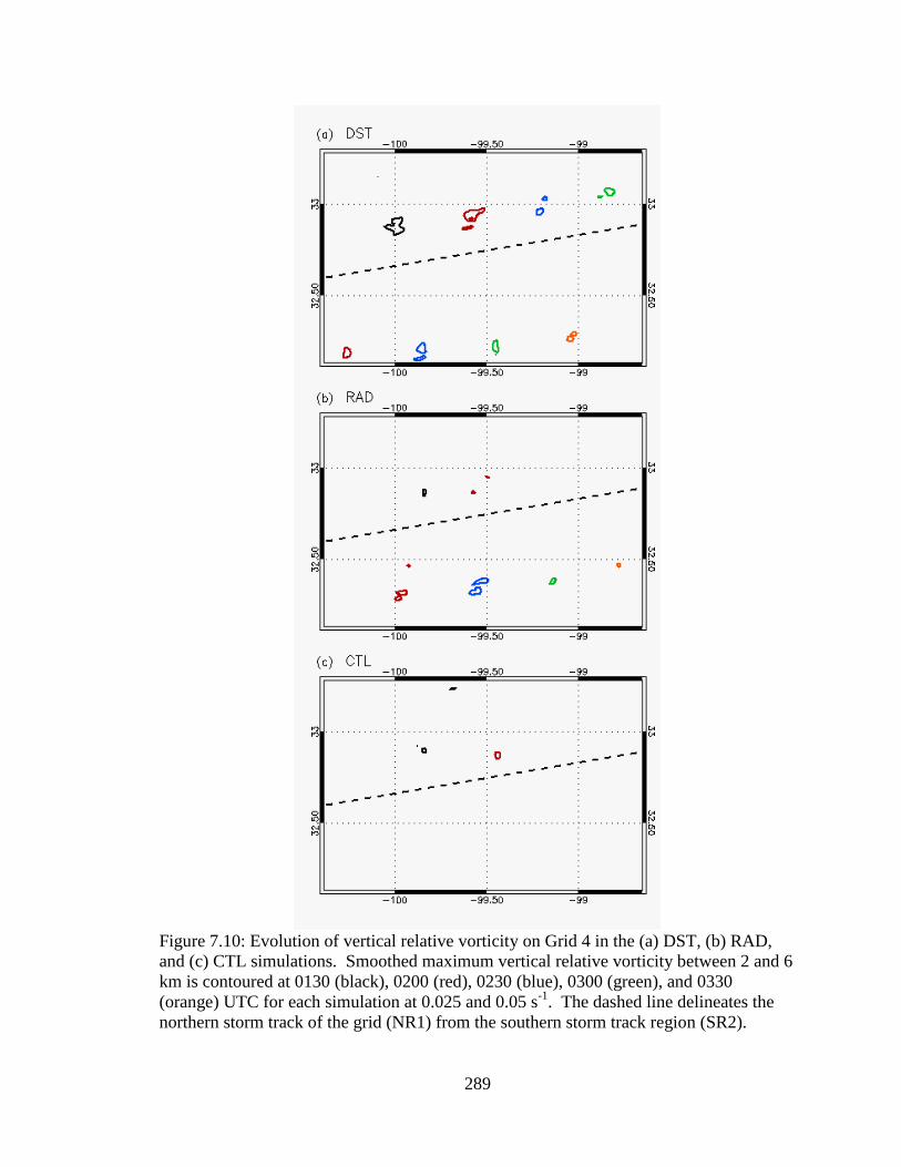
289

Figure 7.10: Evolution of vertical relative vorticity on Grid 4 in the (a) DST, (b) RAD,

and (c) CTL simulations. Smoothed maximum vertical relative vorticity between 2 and 6

km is contoured at 0130 (black), 0200 (red), 0230 (blue), 0300 (green), and 0330

(orange) UTC for each simulation at 0.025 and 0.05 s-1

. The dashed line delineates the

northern storm track of the grid (NR1) from the southern storm track region (SR2).

290

Figure 7.11: Profiles of maximum vertical velocity (column 1), mean updrafts greater

than 1 m s-1

(column 2), minimum vertical velocity (column 3), and mean downdrafts less

than –0.5 m s-1

(column 4) at 0140 (row 1) and 0230 (row 2) UTC on Grid 4 for the DST

(thick solid), RAD (thick dashed), and CTL (thin solid) simulations. Profiles are based

on a 25×25 km region surrounding the location of maximum relative vertical vorticity in

the NR1 region.

291

Figure 7.12: Profiles of maximum vertical velocity (column 1), mean updrafts greater

than 1 m s-1

(column 2), minimum vertical velocity (column 3), and mean downdrafts less

than –0.5 m s-1

(column 4) at 0200 (row 1) and 0230 (row 2) UTC on Grid 4 for the DST

(thick solid), RAD (thick dashed), and CTL (thin solid) simulations. Profiles are based

on a 25×25 km region surrounding the location of maximum relative vertical vorticity in

the SR2 region.

292

Figure 7.13: Precipitation rates on Grid 4 for the DST (column 1), RAD (column 2), and

CTL (column 3) simulations on 16 April at 0130 (row 1), 0200 (row 2), 0230 (row 3),

0300 (row 4), and 0330 UTC (row 5).

293

Figure 7.14: Accumulated precipitation on Grid 3 (row 1) and Grid 4 (row 2) at 5 UTC

on 16 April from the DST (column 1), RAD (column 2), and CTL (column 3)

simulations.

294

Figure 7.15: Time series of (a) grid-cumulative accumulated precipitation and (b)

maximum precipitation rates on Grid 4 for the DST (black), RAD (blue), and CTL (red)

simulations in the NR1 (solid) and SR2 (dashed) regions of the grid.

295

Figure 7.16: Time series of (a) grid-cumulative accumulated precipitation and (b)

maximum precipitation rates on Grid 4 for the DST (thick solid), RAD (thick dashed),

and CTL (thin solid) simulations.

296

Figure 7.17: Near-surface temperature on Grid 2 for the DST (column 1), RAD (column

2), and CTL (column 3) simulations at 2200 UTC on 15 April (row 1) and 0200 UTC on

16 April (row 2). Panels are overlaid with VIC at 0.5 and 5 mm.

297

Figure 7.18: Near-surface temperature on Grid 4 for the DST (column 1), RAD (column

2), and CTL (column 3) simulations at 0200 (row 1), 0230 (row 2), 0300 (row 3), and

0330 (row 4) UTC on 16 April. Panels are overlaid with VIC at 0.5 and 5 mm.

298

Figure 7.19: Mean profiles of cloud1 (row 1) and cloud2 (row 2) droplet mixing ratio

(column 1), number concentration (column 2), and median diameter (column 3) within

updrafts greater than 1 m s-1

on Grid 4 within the NR1 region for the DST (thick solid),

RAD (thick dashed), and CTL (thin solid) simulations at 0200 UTC. Values are based on

the location of maximum vertical relative vorticity and the surrounding 25×25 km region.

299

Figure 7.20: Mean profiles of cloud1 (row 1) and cloud2 (row 2) droplet mixing ratio

(column 1), number concentration (column 2), and median diameter (column 3) within

updrafts greater than 1 m s-1

on Grid 4 within the SR2 region for the DST (thick solid),

RAD (thick dashed), and CTL (thin solid) simulations at 0210 UTC. Values are based on

the location of maximum vertical relative vorticity and the surrounding 25×25 km region.

300

Figure 7.21: Mean profiles of rain (row 1), graupel (row 2), and hail (row 3) number

concentration (column 1) and median diameter (column 2) within updrafts greater than 1

m s-1

, as well as number concentration (column 3) and median diameter (column 4)

within downdrafts stronger than –0.5 m s-1

for the DST (thick solid), RAD (thick dashed),

and CTL (thin solid) simulations at 0200 UTC in the NR1 region. Values are based on

the location of maximum vertical relative vorticity and the surrounding 25×25 km region.

301

Figure 7.22: Mean profiles of rain (row 1), graupel (row 2), and hail (row 3) number

concentration (column 1) and median diameter (column 2) within updrafts greater than 1

m s-1

, as well as number concentration (column 3) and median diameter (column 4)

within downdrafts stronger than –0.5 m s-1

for the DST (thick solid), RAD (thick dashed),

and CTL (thin solid) simulations at 0210 UTC in the SR2 region. Values are based on

the location of maximum vertical relative vorticity and the surrounding 25×25 km region.

302

Figure 7.23: Time series of grid-cumulative (a) cloud1 mass, (b) cloud2 mass, (c) rain

mass below 5 km, (d) pristine ice+snow+aggregate mass above 5 km, (e) graupel mass,

and (f) hail mass on Grid 4 for the DST (black), RAD (blue), and CTL (red) simulations

in the NR1 (solid) and SR2 (dashed) regions of the grid.

303

Figure 7.24: Mean profiles of (a) pristine ice, (b) snow, and (c) aggregate number

concentrations within updrafts greater than 1 m s-1

for the DST (thick solid), RAD (thick

dashed), and CTL (thin solid) simulations at 0210 UTC in the SR2 region.

304

Figure 7.25: Mean sounding comparisons on Grid 2 between the RAD and CTL

simulations at 2300 UTC on 15 April north of 32o latitude and east of –104

o longitude,

within the dust plume where VIC was less than 0.01 mm: (a) grid cells used for mean

calculations; (b) Skew-T log p diagrams of the mean RAD (black) and CTL (blue)

thermodynamic profiles below 500 mb; (c) mean temperature differences between the

RAD and CTL simulations (RAD-CTL); (d) mean profile of mode 1 dust number

concentrations; (e) mean profile of mode 2 dust number concentrations.

305

Figure 7.26: Mean sounding comparisons on Grid 2 between the RAD and CTL

simulations at 2300 UTC on 15 April within the pre-storm environment between 32 and

34o latitude and between –101 and –100

o longitude, where VIC was less than 0.01 mm:

(a) grid cells used for mean calculations; (b) Skew-T log p diagrams of the mean RAD

(black) and CTL (blue) thermodynamic profiles below 500 mb; (c) mean temperature

differences between the RAD and CTL simulations (RAD-CTL); (d) mean profile of

mode 1 dust number concentrations; (e) mean profile of mode 2 dust number

concentrations.

306

Figure 7.27: Grid 4 vertical relative vorticity at 2 km overlaid with storm-relative wind

vectors at the same level (column 1), near-surface vertical relative vorticity overlaid with

near-surface pressure (column 2), near-surface ground-relative wind speeds overlaid with

storm-relative wind vectors at the same level (column 3), and near-surface temperature

overlaid with 1-km total condensate line-contoured at 1 and 4 g kg-1

(column 4) for the

DST NR1 (row 1), DST SR2 (row 2), RAD SR2 (row 3), and CTL NR1 (row 4)

supercells, plotted at the time of maximum vertical vorticity below 6 km; centered over

the location of maximum vertical vorticity. The panels displayed are 10 km×10 km.

307

Figure 7.28: Vertical cross-sections of mean potential temperature overlaid with mean

total condensate greater than 1 g kg-1

(filled pink contoured above 477 m; dashed pink

contour lines below 477 m) and maximum relative vertical vorticity contoured at 0.01,

0.05 (thick), and 0.1 s-1

on Grid 4 for the (a) DST NR1 supercell at 0200 UTC, (b) DST

SR2 supercell at 0220 UTC, (c) RAD SR2 supercell at 0230 UTC, and (d) CTL NR1

supercell at 0150 UTC. The domains are centered over the location of maximum relative

vertical vorticity below 6 km (same as Fig. 7.27). Maximum values of vorticity and

mean values of total condensate and θ are based on the latitude of maximum vorticity

(below 6 km) ± 2.5 km in the latitudinal direction.

308

CHAPTER 8

Summary, Conclusions, and Future Work

8.1 Summary

In this study, multiple three-dimensional, nested grid numerical simulations were

performed using the RAMS model to investigate possible southwestern U.S. desert dust

impacts on severe, tornadic storms in both idealized horizontally-homogeneous scenarios

and a non-idealized, heterogeneous environment of an actual severe storms outbreak.

Initially, two simulations were performed of an idealized supercell storm, where

initial background aerosol concentration profiles were set for a relatively “clean”

continental environment and an aerosol-polluted environment due to the added presence

of a large dust plume. The results of these simulations, presented in Chapter 4, offered a

preliminary look at possible effects of dust and pollutant aerosol acting as CCN and

GCCN on supercell storms. Motivated by the VORTEX findings of Markowski et al.

(2002, 2003), a second ensemble of numerical experiments were conducted, which put

the relative microphysical impacts of aerosols into context with those of CAPE and low-

level moisture for a similar idealized supercell (presented in Chapter 5). In total, five

simulations were performed. In two of them, the initial background CCN concentrations

were set to represent a relatively “clean continental” environment. In two other

simulations, CCN concentrations were increased to represent an aerosol-rich environment

due to the presence of dust or other pollutants. The background water vapor mixing

ratios below 800 mb differed by 20% for each pair of CCN simulations; each simulation

pair was therefore initiated with a 59% difference in CAPE. The fifth simulation was set

309

up with the higher low-level moisture profile but with the same amount of CAPE as the

simulations initialized with the lower low-level moisture profile (created by increasing

the temperatures of the initial sounding above 700 mb). The simulation was initialized

with the “clean continental” background aerosol concentrations.

A final set of numerical experiments was performed in order to simulate possible

dust indirect microphysical and direct radiative impacts on convection during the 15-16

April 2003 severe storms outbreak. These simulations, discussed in Chapter 7, made use

of a comprehensive dust source and transport module (Ginoux et al. 2001; Smith 2007),

wherein a new dust source function was created especially for the southwestern U.S. and

implemented into RAMS for this study. The background CCN was initialized with

heterogeneous fine mode aerosol fields adapted from WRF/Chem model output. Fine

mode dust was activated as CCN using a dust-CCN activation lookup table, based on the

results of a series of parcel simulations where the dust and background aerosol fields

were combined into a single lognormal size distribution represented by bulk values of

number and mass concentration, median radius, and κ parameter. Coarse mode dust was

activated as GCCN using a vertical velocity-activation fraction relationship derived from

the results of a different set of parcel simulations. Heterogeneous ice nucleation was

parameterized by the DeMott et al. (2010) scheme, where dust and non-dust aerosol with

diameters larger than 0.5 µm were allowed to serve as IN at temperatures colder than

0oC. Dust radiative properties were simulated within the Harrington (1997) radiation

scheme, based on the modifications of Stokowski (2005). In one simulation, neither dust

microphysical nor radiative effects were included. In a second simulation, only dust

radiative effects were considered. In a third simulation, both dust radiative and indirect

310

microphysical effects were simulated. The results from the three simulations were

compared in order to evaluate if and how the presence of lofted dust impacted the

strength of resulting convection on 15-16 April 2003.

8.2 Conclusions

In the idealized supercell simulations discussed in Chapter 4, enhanced aerosol

concentrations in the POL simulation reduced warm- and cold-rain processes within the

RFD and FFD. A relatively weak cold-pool was produced at the updraft-downdraft

interface due to reduced evaporative cooling. This provided a favorable environment for

tornadogenesis, where the low-level mesocyclone and near-surface vorticity provided by

the RFD-based gust front remained vertically-stacked. Therefore, the POL supercell

resulted in the formation of an EF-1 tornado while the CLN case failed to produce such a

vortex. Heavier precipitation in the RFD and FFD in the CLN simulation produced more

evaporative cooling, and thus a stronger surface cold-pool that surged and destroyed the

RFD structure. This resulted in a single gust front that advected away more rapidly from

the storm’s core, separating the low-level vorticity source from the parent storm. The

results were consistent with the findings of Markowski et al. (2002, 2003) and Snook and

Xue (2008) regarding the importance of cold-pool dynamics and the vertical alignment of

vertical vorticity within a supercell to tornadogenesis. The results from this single,

idealized set of simulations suggested that “all else being equal,” a polluted environment

is more favorable for tornadogenesis.

In the idealized supercell simulations discussed in Chapter 5, the right moving

supercell produced a tornado-like vortex in each simulation. However, considerable

311

differences were found with respect to storm microphysics and low to mid-level

dynamics. The combined effects of increased ambient low-level moisture and increased

CAPE (HM simulations) resulted in spatially larger storms with stronger peak updrafts

and stronger low-level downdrafts compared to the LM simulations. The dusty

simulations produced slightly greater peak updrafts due to the presence of more

supercooled liquid water aloft and associated latent heat of freezing. The HM storms

produced noteably stronger precipitation, which resulted in greater evaporation and

associated cooling, thus producing stronger cold-pools at the surface associated with both

the forward and rear flank downdrafts. The higher CCN concentrations in the dusty

simulations reduced warm rain and yielded more supercooled water aloft, creating larger

anvils with less ice mass available for precipitation. This resulted in lower hail number

concentrations. However, raindrops and hailstones grew to larger sizes. The supercells

from the dusty simulations underwent less evaporative cooling within downdrafts as a

result, and produced weaker low level downdrafts and weaker, warmer cold-pools

compared to the clean simulations. With greater terminal fall velocities, the larger

hydrometeors fell nearer to the storm’s core, which positioned the coldest region of the

cold-pool closer to the main updraft. Tornadogenesis was related to the size, strength,

and location of the FFD- and RFD-based cold-pools. The combined influence of low-

level moisture and CAPE played a noticeably larger role in the tornadogenesis process

compared to the aerosol influence. However, the aerosol effect was still evident.

Changing the low-level moisture profile resulted in changes to storm size and

precipitation totals, but altering the background available CCN concentrations resulted in

large differences in storm microphysics and the location of precipitation cores. It was the

312

combined effect that determined the strength and location of the cold-pool, which in turn,

determined vortex initiation and duration. The findings from the CLN-WETb simulation

indicated that increasing the ambient relative humidity profile at low levels without

affecting CAPE still resulted in a stronger cold-pool that hindered the tornadogenesis

process, as the increased moisture supply at low levels led to increased precipitation and

strong evaporative cooling within downdrafts. The general results of Markowski et al.

(2002, 2003) were consistent with those of this model ensemble. The strongest, longest-

lived tornado-like vortices were associated with warmer and weaker cold-pools, higher

CAPE, lower CIN, and thus less negative buoyancy in the near-vortex environment

compared to those storms that produced shorter-lived, weaker vortices.

The results from the simulations of Chapters 4 and 5 suggested that altering

background CCN concentrations can have large impacts on precipitation rates and

resulting cold-pool intensity, which in turn, can influence the likelihood of

tornadogenesis via storm undercutting, a known potential failure mechanism for

tornadogenesis (Wilhelmson and Klemp 1978; Weisman and Klemp 1982; Brooks et al.

1993, 1994a,b; Gilmore and Wicker 1998). However, if conditions are such that storm

undercutting is unlikely even with changes to the background aerosol, aerosol effects are

far more complex but will have a much smaller impact compared to the combined effects

of low-level moisture and CAPE.

In the 15-16 April case study, all three simulations produced a north-south

oriented convective line with embedded supercell convection. In the DST simulation,

cloud1 droplet nucleation was greatly reduced due to the presence of fine mode dust

reducing bulk aerosol hygroscopicity. Therefore, cloud1 droplets were of smaller sizes

313

than those found in the RAD and CTL simulations. This reduced cloud droplet self-

collection, which further resulted in smaller cloud2 droplet concentrations of smaller size

in the DST simulations. The impact of the fine mode dust reducing CCN nucleation

played a far greater role on the resulting cloud2 droplet spectra than of the coarse mode

dust serving at times as GCCN. The warm rain process was severely reduced in the DST

simulation, even though raindrops grew to larger sizes than those in the RAD and CTL

simulations. The small cloud drops were sent into the mixed-phase region of the updraft,

which upon freezing, enhanced latent heating and helped to strengthen peak updrafts

within DST convection. The rime-splinter process was favored in the RAD and CTL

simulations due to the presence of cloud1 droplets with diameters greater than 24µm,

which yielded high concentrations of small pristine ice crystals. In contrast, aggregation

was most efficient in the DST simulation. Dust served as IN in the DST simulation as

well. However, this process was offset by the enhanced Hallett-Mossop rime-splintering

in the RAD and CTL cases. With considerably more ice mass aloft in the DST

simulations and numerous small cloud drops available for riming, the DST simulation

produced the highest graupel and hail concentrations but of relatively small size due to

reduced riming efficiencies and riming rates. The graupel and hail that formed in the

RAD and CTL simulations grew to larger sizes than in the DST simulation, because the

presence of larger cloud drops and higher raindrop number concentrations resulted in

greater riming efficiency and thus higher riming rates.

The DST simulation yielded the lowest rainfall rates and accumulated

precipitation, as much of the total water mass within the convective cells were in the form

of aggregates and small graupel particles that remained aloft and were transported into

314

the anvil region rather than falling as precipitation. However, the DST downdraft regions

were associated with higher number concentrations of smaller graupel and hail particles.

With such high surface area-to-volume ratios, associated melting and evaporation of

these small hydrometeors falling below the melting level resulted in enhanced cooling,

increased negative buoyancy, and at times, stronger downdrafts than those produced in

the RAD and CTL simulations. However, this effect was often not enough to create

stronger downdrafts than what was produced in the RAD and CTL simulations where

precipitation was greater overall. The combined effects of warm rain efficiency, ice

production, and hydrometeor size together controlled the overall evolution of cold-pools

and storm structure. The RAD and CTL convective lines initially produced heavy warm

rain precipitation on Grid 4 between 0040 and 0200 UTC, while the DST simulation saw

a reduction in warm rain production. As a result, the RAD and CTL simulations

produced widespread cold-pools of varying temperature, which initially hindered the

formation of long-lived, classical type supercells. The DST convective line was

associated with reduced rainfall and multiple long-lived supercells. The RAD simulation

eventually produced a strong, persistent supercell in the SR2 sub domain, which

exhibited many similar features as that produced by the DST simulation in the same

region.

Comparisons between the RAD and CTL simulation revealed that dust radiative

influences played a role in developing convection. The increased absorption of solar

radiation within the lofted dust plume in the RAD simulation warmed the dust layer over

time, which reduced the amount of radiation that reached the surface and therefore

resulted in slight cooling at the surface compared to the CTL simulation. This created a

315

steeper lapse rate and thus increased atmospheric stability in the RAD simulation within

the lowest 2 km. Dew point values within the dust plume below 2 km were also slightly

lower in the RAD simulation than those in the CTL case, due to reduced surface water

vapor fluxes. Consistent with the findings of Ziegler et al. (2010), the CTL simulation

generally produced more widespread convection and precipitation within the NR1 region

prior to 0230 UTC, while the RAD simulation produced the strongest convective cores.

In addition, the RAD SR2 region produced a long-lived supercell while the CTL

simulation failed to spawn any long-lived supercell storms. However, with reduced pre-

convective low-level moisture in the RAD simulation, the CTL simulation had higher

potential for warm rain production, at least initially, and the CTL simulation was

associated with the maximum precipitation rates prior to 0115 UTC. This suggested that

slight variations in available low-level moisture between simulations, at least towards the

leading edge of the dust plume, contributed to resulting convection.

All three simulations produced convection that exhibited similar features to the

actual 15-16 April convective line. With reduced rainfall overall, the DST simulation

possessed the greatest severe storm potential, producing two long-lived supercells on

Grid 4. The RAD and CTL simulations yielded higher precipitation rates, more

precipitation accumulation, greater riming efficiencies, and larger hail. However, the

RAD simulation produced only one supercell-like storm on Grid 4 that lasted longer than

30 min. The CTL simulation failed to produce any long-lived supercells. These results

suggest that dust indirect microphysical effects and direct radiative impacts on severe

convection can be important. However, additional work is needed to address the

robustness of these results and to better isolate potential dust influences on severe storms.

316

8.3 Future Work

While the 15-16 April simulations suggested that lofted desert dust from the

southwestern U.S. may impact the severity of storm outbreaks in the Southern Plains via

indirect microphysical and direct radiative effects on convection and subsequent cold-

pool production, the horizontal grid spacing on Grid 4 was too coarse to assess possible

impacts on tornadogenesis. Furthermore, it was difficult to isolate specific aerosol effects

on the simulated convective line, because the extent of the role that dust and other

aerosols played will likely vary among individual convective cells. Therefore, idealized

simulations similar to those presented in Chapters 4 and 5 should be performed for an

individual supercell, where the model is initialized with a horizontally homogeneous

environment based on the pre-convective mesoscale environment associated with the 15-

16 April 2003 outbreak. This would allow for horizontal grid spacing on the order of 100

m and explicit simulation of the tornadogenesis process. In addition, the effects of dust

serving as CCN, GCCN, and IN could be further isolated.

Various computational restrictions must be taken into account when considering

the merit of the 15-16 April case simulations. Given that Grid 2 was forced to cover a

larger domain than originally planned in order to better resolve the convective line of

interest, Grid 4 was limited to 500-m horizontal spacing due to computational demands.

In addition, the double-moment microphysics package that was used is incapable of

producing hail sizes comparable to what is found in deep convection (diameters greater

than 1 cm). As a result, RAMS simulations using this scheme cannot produce hail that

reaches the surface. Lastly, it is always difficult to generalize the results of a single case.

RAMS version 6 is now available (Stephen Saleeby, personal communication), capable

317

of running on 64-bit computers, no longer limited by a maximum memory storage

allowance. This means that simulations run with RAMS version 6 can make use of larger

domains and finer grid spacing. In addition, Loftus (2012) has implemented a 3-moment

hail model into RAMS 4.3, which allows for the simulation of more realistic hail size

distributions, larger hail, and thus hail accumulation at the surface. In the future, the

WRF/Chem-based treatment of aerosol in RAMS 4.3 and the triple-moment hail scheme

should be implemented into RAMS version 6. Once installed, the 15-16 April case study

as well as other possible dust cases should be simulated with RAMS version 6 using a

single grid with horizontal grid spacing on the order of 200 m, making use of the 3-

moment hail scheme.

The idealized simulations performed in Chapters 4 and 5 were for a single

sounding. In order to determine the robustness of the results from those simulations as

well as to determine which storm and background aerosol environments are most likely

to be influenced by dust microphysical effects, another idealized model ensemble should

be performed using RAMS version 6, where parameters such as CAPE, vertical wind

shear, low-level moisture, CCN, GCCN, and IN concentrations are all varied among the

simulations to determine when aerosols are most likely to impact tornadogenesis.

318

REFERENCES

Abdul‐Razzak, Hayder and Steven J. Ghan, 2002: A parameterization of aerosol

activation 3. Sectional representation. J. Geophys. Res., 107(D3),

doi:10.1029/2001JD000483.

Achtemeier, G. L., 1975: Doppler velocity and reflectivity morphology of a severe left-

moving split thunderstorm. Preprints, 16th Conf. Radar Meteor., Houston, Amer.

Meteor. Soc., 93-98.

Ackerman, S.A., 1997. Remote sensing aerosols using satellite infrared observations.

J. Geophys. Res., 102, (D14), 17069-17079.

AFCCC (Air Force Combat Climatology Center), 2004: Rules of Thumb for Dust

Storms. AFCC Strategic Weather Now, March 2004, 1, No. 3.

Albrecht, Bruce A., 1989: Aerosols, cloud microphysics, and fractional cloudiness.

Science, 245, 1227‐1230.

Andreae, M. O., and D. Rosenfeld, 2008: Aerosol–cloud–precipitation interactions. Part

1: The nature and sources of cloud‐active aerosols. Earth Sci. Rev., 89,

doi:10.1016/j.earscirev.2008.03.001.

Arakawa, A., and V. Lamb, 1981: A potential enstrophy and energy conserving scheme

for the shallow water equations. Mon. Wea. Rev., 109, 18–36.

Archuleta, C.M., P. J. DeMott, and S. M. Kreidenweis, 2005: Ice nucleation by

surrogates for atmospheric mineral dust and mineral dust/sulfate particles at cirrus

temperatures. Atmospheric Chemistry and Physics, 5, 2617-2634.

Auer, A. H. Jr., D. L. Veal, and J. D. Marwitz, 1969: Observations of Ice Crystal and Ice

Nuclei Concentrations in Stable Cap Clouds. J. Atmos. Sci., 26, 1342-1343.

Austin, P., Y. Wang, R. Pincus, and V. Kujala, 1995: Precipitation in stratocumulus

clouds: Observational and modeling results. J. Atmos. Sci., 52, 2329-2352.

Barkstrom, B. R., 1978: Some effects of 8-12 um radiant energy transfer on the mass and

heat budgets of cloud droplets. J. Atmos. Sci., 35, 665-673.

Barnes, S. L., 1964: A technique for maximizing details in numerical weather map

analysis. J. Appl. Meteor., 3, 396-409.

Barnes, S. L., 1978: Oklahoma thunderstorms on 29-30 April, 1970. Part II: radar-

observed merger of twin hook echoes. Mon. Wea. Rev., 106, 685-696.

319

Barnes, S. L., and C. W. Newton, 1986: Thunderstorms in the synoptic setting.

Thunderstorm Morphology and Dynamics, E. Kessler, ed., University of Oklahoma

Press, 615 pp.

Baron, P. A., and K. Willeke, 2001: Aerosol measurement: Principles, techniques and

applications. Second Edition. Wiley-Interscience Inc.

Berezinski, N., G. Stepanov, V. Khorguani, 1986: Height variation of relative ice-

forming activity of natural aerosol. Meteorologia 1 Gidrologia. 12, 102-105.

Bergeron, T., 1933: On the physics of clouds and precipitation, in Proc. 5th

Assembly

UGGI, Vol. 2., Lisbon.

Bigg, E.K., 1953: The Supercooling Of Water. Proceedings Of The Physical Society Of

London Section B, 66(404): 688-694.

Bigg, E. K., 1988: Secondary ice nucleus generation by silver iodide applied to the

ground. J. Appl. Meteor., 27, 453-457.

Bigg, E. K., 1990: Aerosol over the southern ocean, Atmos. Res., 25, 583-600

Bigg, E. K., and E. Turton, 1988: Persistent effects of cloud seeding with silver iodide. J.

Appl. Meteor., 27, 505-514.

Binkowski, Francis S. and Uma Shankar, 1995: The Regional Particulate Matter Model:

1. Model description and preliminary results. J. Geophys. Res., 100(D12), 26,191‐26,209.

Bluestein, H. B., 1984: Further examples of low-precipitation severe thunderstorms. Mon.

Wea. Rev., 112, 1885-1888.

Bluestein, H. B., 1985: The formation of a ‘landspout’ in a ‘broken-line’ squall line in

Oklahoma. Preprints, 14th

Conf. On Severe Local Storms, Indianapolis, IN, Amer.

Meteor. Soc., 267-270.

Bluestein, H. B., 1992: Synoptic-Dynamic Meteorology in Midlatitudes. Oxford

University Press, New York, p. 335.

Bluestein, H. B., 2005: A review of ground-based, W-band Doppler-radar observations of

tornadoes and dust devils. Dyn. Atmos. Oceans, 40, 163-188.

Bluestein, H. B., and C. R. Parks, 1983: A synoptic and photographic climatology of low-

precipitation severe thunderstorms in the southern plains. Mon. Wea. Rev., 111, 2034-

2046.

Bluestein, H. B., and G. R. Woodall, 1990: Doppler-radar analysis of a low-precipitation

severe storm. Mon. Wea. Rev., 118, 1640-1664.

320

Borys, R. D., D. H. Lowenthal, M. A. Wetzel, F. Herrera, A. Gonzalez, and J. Harris,

1998: Chemical and microphysical properties of marine stratiform cloud in the North

Atlantic. J. Geophys. Res., 103, 22073-22085.

Borys, R. D., D. H. Lowenthal, S. A. Cohn, and W. O. J. Brown, 2003: Mountaintop and

radar measurements of anthropogenic aerosol effects on snow growth and snowfall rate.

Geophys. Res. Lett., 30(10), doi:10.1029/2002GL016855.

Borys, R. D., D. H. Lowenthal, and D. L. Mitchell, 2000: The relationship among cloud

microphysics, chemistry, and precipitation rate in cold mountain clouds. Atmos. Environ.,

34, 2593‐2602.

Brady, R. H., and E. J. Szoke, 1989: A case study of non-mesocyclone tornado

development in northeast Colorado: Similarities to waterspout formation. Mon. Wea.

Rev., 117, 843-856.

Braham, R. R., Jr., 1964: What is the role of ice in summer rain-showers? J. Atmos. Sci.,

21, 640-646.

Braham, R. R., Jr., R. G. Semonin, A. H. Auer, S. A. Changnon Jr., and J. M. Hales,

1981: Summary of urban effects on clouds and rain. METROMEX: A review and

summary, Meteor. Monogr., 40, 141-152.

Brandes, E. A., 1978: Mesocyclone evolution and tornadogenesis: Some observations.

Mon. Wea. Rev., 106, 995-1011.

Brooks, H. E., C. A. Doswell III, and R. Davies-Jones, 1993: Environmental helicity and

the maintenance and evolution of low-level mesocyclones. The Tornado: Its structure,

dynamics, prediction, and hazards. Geophys. Monogr., No. 79, Amer. Geophys. Union,

97-104.

Brooks, H. E., C. A. Doswell III, and R. B. Wilhelmson, 1994: The role of

midtropospheric wind in the evolution and maintenance of low-level mesocyclones. Mon.

Wea. Rev., 122, 126–136.

Brooks, H. E., C. A. Doswell III, and J. Cooper, 1994b: On the environments of tornadic

and nontornadic mesocyclones. Wea. Forecasting, 9, 606–618.

Brooks, N., 2000: Dust-climate interactions in the Sahel-Sahara zone of Northern Africa,

with particular reference to late twentieth century Sahelian drought. Ph.D. Dissertation,

Climatic Research Unit, University of East Anglia, Norwich.

Browning, K. A., 1964: Airflow and precipitation trajectories within severe local storms

which travel to the right of the winds. J. Atmos. Sci., 21, 634–639.

Browning, K. A., 1968: The organization of severe local storms. Weather, 23, 429-434.

321

Brown, P. N., G. D. Byrne, and A. C. Hindmarsh, 1989: Vode –A variable-coefficient

ODE solver. SIAM J. Sci. Stat. Comp., 10(5), 1038–1051.

Burgess, D. W., and R. J. Donaldson, Jr, 1979: Contrasting tornadic storm types.

Preprints, 11th

Conf. on Severe Local Storms, Kansas City, MO, Amer. Meteor. Soc.,

189-192.

Burgess, D. W., and R. P. Davies-Jones, 1979: Unusual tornadic storms in eastern

Oklahoma on 5 December, 1975. Mon. Wea. Rev., 107, 451-457.

Burgess, D. W., V. T. Wood, and R. A. Brown, 1982: Mesocyclone evolution statistics.

Preprints, 12th

Conf. on Severe Local Storms, Amer. Meteor. Soc., 84-89.

Burgess, D. W., R. A. Brown, L. R. Lemon, and C. R. Safford, 1977: Evolution of a

tornadic thunderstorm. Preprints, 10th Conf. On Severe Local Storms, Omaha, NE, Amer.

Meteor. Soc., 84–89.

Chate, D. M., and T. S. Pranesha, 2004: Field measurements of sub-micron aerosol

concentration during cold season in India. Current Sci., 86, 1610-1613.

Chate, D. M., 2005: Study of scavenging of submicron-sized aerosol particles by

thunderstorm rain events. Atmos. Environ., 39, 6608-6619.

Chylek, P., M. K. Dubey, U. Lohmann, V. Ramanathon, Y. J. Kaufman, G. Lesins, J.

Hudson, G. Altmann, and S. C. Olsen, 2006: Aerosol indirect effect over the Indian

Ocean. Geophys. Res. Lett., 33, doi:10.1029/2005GL025397.

Clark, T. L., 1977: A small scale dynamic model using a terrain-following coordinate

transformation. J. Comput. Phys., 24, 186-215.

Clark, T. L., and R. D. Farley, 1984: Severe downslope windstorm calculations in two

and three spatial dimensions using anelastic interactive grid nesting: A possible

mechanism for gustiness. J. Atmos. Sci., 41, 329–350.

Cober, S. G., and R. List, 1993: Measurements of the heat and mass transfer parameters

characterizing conical graupel growth. J. Atmos. Sci., 50, 1591-1609.

COMET (Cooperative Program for Operational Meteorology), 2003: Mesoscale Primer.

Forecasting Dust Storms. University Corporation for Atmospheric Research. Sections

3.1.1, 3.1.2, 3.2.2, 3.2.5, 3.3.3, 5.2.1, 6.3.

Cooper, W. A., 1995: Ice formation in wave clouds: Observed enhancement during

evaporation. Proc. Conf. Cloud Physics, Dallas, Amer. Meteor. Soc., 147-152.

Cotton, W. R., 1972: Numerical simulation of precipitation development in supercooled

cumuli-Part I. Mon. Wea. Rev., 100, 757–763.

322

Cotton, R. J., and P. R. Field, 2002: Ice nucleation characteristics of an isolated wave

cloud. Q. J. Roy. Met. Soc., 128, 2417-2437.

Cotton, W. R., and S. Yuter, 2007: Principles of cloud and precipitation formation. In:

Levine, Z., Cotton, W. (Eds.), WMO/IUGG International Aerosol Precipitation Science

Assessment Group (IAPSAG) Report: Aerosol Pollution Impact on Precipitation: a

Scientific Review. World Meteorological Organization, pp. 31-68.

Cotton, W. R., R. A. Pielke Sr., R. L. Walko, G. E. Liston, C. J. Tremback, H. Jiang, R.

L. McAnelly, J. Y. Harrington, M. E. Nicholls, G. G. Carrio, and J. P. McFadden, 2003:

Rams 2001: Current status and future directions. Meteor. Atmos. Phys., 82, 5-29.

Cotton, W. R., R. McAnelly, G. Carrio, P. Mielke, and C. Hartzell, 2006: Simulations of

snowpack augmentation in the Colorado Rocky Mountains. J. Wea. Mod., 38, 58-65.

Cubison, M.J., B. Ervens, G. Feingold, K.S. Docherty, I.M. Ulbrich, L. Shields, K.

Prather, S. Hering, J.L. Jimenez, 2008: The influence of chemical composition and

mixing state of Los Angeles urban aerosol on CCN number and cloud properties. Atmos.

Chem. Phys., 8, 5649‐5667.

Danielson, E. F., 1977: Inherent difficulties in hail probability prediction. Meteor.

Monogr., 16, No. 38, Amer. Met. Soc., Boston, MA, G. B. Foote and C. A. Knight, Eds.,

135-143.

Danielson, E. F., and V. A. Mohnen, 1977: Project DUSTORM report: Ozone transport,

in situ measurements and meteorological analysis of tropopause folding. J. Geophys.

Res., 82, 5867-5877.

Davenport, H. M., and L. K. Peters, 1978: Field studies of atmospheric particulate

concentration changes during precipitation. Atmos. Environment, 12, 997-1008.

Davies-Jones, R. P., 1982a: A new look at the vorticity equation with application to

tornadogenesis. Preprints, 12th Conf. on Severe Local Storms, San Antonio, TX, Amer.

Meteor. Soc., 249–252.

Davies-Jones, R. P., 1982b: Observational and theoretical aspects of tornadogenesis.

Intense Atmospheric Vortices, L. Bengtsson and J. Lighthill, Eds., Springer-Verlag, 175–

189.

Davies-Jones, R. P., 1984: Streamwise vorticity: The origin of updraft rotation in

supercell storms. J. Atmos. Sci., 41, 2991-3006.

Davies-Jones, R. P., 1985: Dynamical interaction between an isolated convective cell and

a veering environmental wind. Preprints, 14th

Conf. on Severe Local Storms, Indianapolis,

IN, Amer. Meteor. Soc., 588-592.

323

Davies-Jones, R. P., 1996: Formulas for the barotropic and baroclinic components of

vorticity with applications to vortex formation near the ground. Preprints, Seventh Conf.

on Mesoscale Processes, Reading, United Kingdom, Amer. Meteor. Soc., 14-16.

Davies-Jones, R. P., 2000: Can the hook echo instigate tornadogenesis barotropically?

Preprints, 20th Conf. on Severe Local Storms, Orlando, FL, Amer. Meteor. Soc., 269–272.

Davies-Jones, R., and D. W. Burgess, 1990: Test of helicity as a tornado forecast

parameter. Preprints, 16th Conf. on Severe Local Storms, Kananaskis Park, AB, Canada,

Amer. Meteor. Soc., 588-592.

Davies-Jones, R. P., 2006: Tornadogenesis in supercell storms: What we know and what

we don’t know. Preprints, Symp. on the Challenges of Severe Convective Storms, Atlanta,

GA, Amer. Meteor. Soc., 2.2.

Davies-Jones, R. P., 2008: Can a descending rain curtain in a supercell instigate

tornadogenesis barotropically? J. Atmos. Sci., 65, 2469-2497.

Davies-Jones, R. P., and H. E. Brooks, 1993: Mesocyclogenesis from a theoretical

perspective. The Tornado: Its Structure, Dynamics, Prediction, and Hazards, Geophys.

Monogr., 79, Amer. Geophys. Union, 105–114.

Davies-Jones, R. P., R. J. Trapp, and H. B. Bluestein, 2001: Tornadoes and Tornadic

Storms. Severe Convective Storms, Meteor. Monograph, 28, Amer. Meteor. Soc., Boston,

MA, 126-221.

Deardorff, J. W., 1980: Stratocumulus-capped mixed layers derived from a three-

dimensional model. Bound.-Layer Meteor., 18, 495-527.

DeFries, R. S., and J. R. Townshend, 1994: NDVI-derived land cover classification at a

global scale. Int. J. Remote Sens., 15, 3567-3586.

DeMott, P. J., A. J. Prenni, X. Liu, S. M. Kreidenweis, M. D. Petters, C. H. Twohy, M. S.

Richardson, T. Eidhammer, and D. C. Rogers, 2010: Predicting global atmospheric ice

nuclei distributions and their impacts on climate. P. Natl. Acad. Sci. USA, 107, 11217-

11222.

DeMott, P.J., D.J. Cziczo, A. J. Prenni, D. M. Murphy, S. M. Kreidenweis, D. S.

Thomson, R. Borys, and D.C. Rogers, 2003: Measurements of the concentration and

composition of nuclei for cirrus formation. Proceedings of the Nat. Academy of Sciences,

100, No. 25, 14655‐14660.

DeMott, P. J., M. D. Petters, A. J. Prenni, C. M. Carrico, S. M. Kreidenweis, J. L. Collett,

and H. Moosmuller, 2009: Ice nucleation behavior of biomass combustion particles at

cirrus temperatures. J. Geophys. Res., 114, D16205, doi: 10.1029/2009jd012036.

324

DeMott, P. J., Y. Chen, S. M. Kreidenweis, D. C. Rogers, and D. E. Sherman, 1999: Ice

formation by black carbon particles, Geophys. Res. Lett., 26(16), 2429-2432.

DeMott, P. J., K. Sassen, M. R. Poellot, D. Baumgardner, D. C. Rodgers, S. D. Brooks,

A. J. Prenni, and S. M. Kreidenweis, 2003: African dust aerosols as atmospheric ice

nuclei. Geophys. Res. Lett., 30, No. 14, 1732, doi:10.1029/2003GL017410.

DeMott, P. J., M.P. Meyers, and W. R. Cotton, 1994: Parameterization and impact of ice

initiation processes relevant to numerical model simulations of cirrus clouds. J. Atmos.

Sci., 41, 77-90.

Dong, Y.Y., R.G. Oraltay, R.G. and J. Hallett, 1994: ice particle generation during

evaporation. Atmos. Res. 32, 45-53.

Doswell, C. A., III, 1985: The operational meteorology of convective weather. Vol II:

Storm-scale analysis. NOAA Tech. Memo. ERL ESG-15, 240 pp.

Doswell, C. A., III, and D. W. Burgess, 1993: Tornadoes and tornadic storms: A review

of conceptual models. The Tornado: Its Structure, Dynamics, Prediction, and Hazards,

Geophys. Monogr., No. 79, Amer. Geophys. Union, 161–172.

Doswell, C. A., III, A. R. Moller, and R. Przybylinski, 1990: A unified set of conceptual

models for variations on a supercell theme. Preprints, 16th Conf. on Severe Local Storms,

Kananaskis Park, AB, Canada, Amer. Meteor. Soc., 40–45.

Droegemeier, K. K., S. M. Lararus, and R. Davies-Jones, 1993: The influence of helicity

on numerically simulated convective storms. Mon. Wea. Rev., 121, 2005–2029.

Dufour, L., and R. Defay, 1963: Thermodynamics of Clouds, Ch. VIII, Academic, New

York.

Dunion, J. P. and C. S. Velden, 2004: The impact of the Saharan Air Layer on Atlantic

tropical cyclone activity. Bull. Amer. Meteor. Soc., 353-365.

Durant, A.J. and R.A. Shaw, 2005: Evaporation freezing by contact nucleation inside-out.

Geophys. Res. Lett., 32, doi:10.1029/2005GL024175.

Eagan, R. C., P. V. Hobbs, and L. F. Radke, 1974: Particle emissions from a large Kraft

paper mill and their effects on the microphysical structure of warm clouds. J. Appl.

Meteor., 13, 535-552.

Eidhammer, T., P. J. DeMott, and S. M. Kreidenweis, 2009: A comparison of

heterogeneous ice nucleation parameterizations using a parcel model framework, J.

Geophys. Res.-Atmos., 114, D06202, doi:10.1029/2008JD011095.

325

Ervens, B., M. Cubison, E. Andrews, G. Feingold, J. A. Ogren, J. L. Jimenez, P. DeCarlo,

and A. Nenes, 2007: Prediction of cloud condensation nucleus number concentration

using measurements of aerosol size distributions and composition and light scattering

enhancement due to humidity. J. Geophys. Res., 112, D10S32,

doi:10.1029/2006JD007426.

Facchini, M. C., M. Mircea, S. Fuzzi, and R. J. Charlson, 1999: Cloud albedo

enhancement by surface-active organic solutes in growing droplets. Nature, 401, 257-

259.

Fan, S.-M., L. W. Horowitz, H. L. II, and W. J. Moxim, 2004: Impact of air pollution on

wet deposition of mineral dust. J. Geoph. Res., 31, L02104, doi:10.1029/2003GL018501.

Feingold, G., W. R. Cotton, S. M. Kreidenweis, and J. T. Davis, 1999: The impact of

giant cloud condensation nuclei on drizzle formation in stratocumulus: Implications for

cloud radiative properties. J. Atmos. Sci., 56, 4100-4117.

Field, P. R., R. J. Cotton, K. Noone, and coauthors, 2001: Ice nucleation in orographic

wave clouds: Measurements made during INTACC, Quart. J. Royal Meteorol. Soc., 127,

1493-1512.

Findeisen, W., 1938: Die kolloidmeteorologisch Vorgänge bei der Niederschlagsbildung.

Met. Z55, 121-132.

Fletcher, N.H., 1958: Size Effect in Heterogeneous Nucleation. J. of Chemical

Physics, 29(3), 572-576.

Fletcher, N.H., 1962: The Phys. of Rainclouds, Cambridge University Press, Cambridge,

U.K., 242 pp.

Foote, G. B., 1984: A study of hail growth utilizing observed storm conditions. J. Climate

Appl. Meteor., 23, 84-101.

Fujita, T. T., 1957: Three-dimensional mesoanalysis of a squall line. Res. Rep. No. 1,

Contract DA-36-039- SC-64656, Illinois State Water Survery, 19 pp.

Fujita, T. T., 1963: Analytical mesometeorology: A review. Severe Local Storms, Meteor.

Monogr., 27, Amer. Meteor. Soc., 77–125.

Fujita, T. T., 1971: Proposed mechanism of suction spots. Weatherwise, 23, 161-173.

Fujita, T. T., 1981: Tornadoes and downbursts in the context of generalized planetary

scales. J. Atmos. Sci., 38, 1511-1534.

326

Gagin, A., 1965: Ice Nuclei, their physical characteristics and possible effect on

precipitation initiation: Proc. Tokyo-Sapporo Int. Conf. On Cloud Physics, Sapporo,

Japan, Int. Assoc. of Meteor. and Atmos. Phys. of the IUGG, 155-162.

Gal-Chen, T., and R. C. J. Somerville, 1975: On the use of a coordinate transformation

for the solution of the Navier- Stokes equations. J. Comput. Phys., 17, 209–228.

Gaudet, B. J., and W. R. Cotton, 2006: Low-level mesocyclonic concentration by non-

axisymmetric processes. Part I: Supercell and mesocyclone evolution. J. Atmos. Sci., 63,

1113-1133.

Gaudet, B. J., W. R. Cotton, and M. T. Montgomery, 2006: Low-level mesocyclonic

concentration by nonaxisymmetric transport: II. Vorticity dynamics. J. Atmos. Sci., 63,

1134–1150.

Georgii, H. W. and E. Kleinjung, 1967: Relations between the chemical composition of

atmospheric aerosol particles and the concentration of natural ice nuclei. J. Rech.

Atmos., 3, 145-156.

Gillette, D. A., and R. Passi, 1988: Modeling dust emission caused by wind erosion. J.

Geoph. Res., 93, 14,233-14,242.

Gilmore, M. S., and L. J. Wicker, 1998: The influence of midtropospheric dryness on

supercell morphology and evolution. Mon. Wea. Rev., 126, 943–958.

Gilmore, M. S., J. M. Straka, and E. N. Rasmussen, 2004: Precipitation uncertainty due to

variations in precipitation particle parameters within a simple microphysics scheme. Mon.

Wea. Rev., 132, 2610-2627.

Ginoux, P., M. Chin, I. Tegen, J. M. Prospero, B. Holden, O. Dubovik, and S.-J. Lin,

2001: Sources and distributions of dust aerosols simulated with the gocart model. J.

Geoph. Res., 106, 20255-20273.

Gitlin, S. N., 1978: Microprobe Analysis of Project DUSTORM Hailstone Samples. J.

Atmos. Sci., 17, 64-72.

Gokhale, N.R., and J.D. Spengler, 1972: Freezing of freely suspended water drops by

contact nucleation. J. Appl. Meteor., 11, 157–160.

Gong, S., and L. A. Barrie, 2007: The distribution of atmospheric aerosols: Transport,

transformation and removal. In: Levine, Z., Cotton, W. (Eds.), WMO/IUGG

International Aerosol Precipitation Science Assessment Group (IAPSAG) Report:

Aerosol Pollution Impact on Precipitation: a Scientific Review. World Meteorological

Organization, pp. 127-187.

327

Gong, S. L., X. Y. Zhang, T. L. Zhao, I. G. McKendry, D. A. Jaffe, and N. M. Lu, 2003:

Characterization Of Soil Dust Distributions In China And Its Transport During ACE-

ASIA 2. Model Simulation and Validation. J. Geophys. Res., 108, 4262,

doi:4210.1029/2002JD002633.

Grasso, L. D., 1996: Numerical simulation of the May 15 and April 26, 1991 tornadic

thunderstorms. Ph.D. dissertation, Atmos. Sci. Paper 596, Colorado State University, 151

pp.

Grasso, L. D., 2000: The dissipation of a left-moving cell in a severe storm environment.

Mon. Wea. Rev., 128, 2797–2815.

Grasso, L. D., and W. R. Cotton, 1995: Numerical simulation of a tornado vortex. J.

Atmos. Sci., 52, 1192–1203.

Greenan, B. J. W., and R. List, 1995: Experimental closure of the heat and mass transfer

theory of spheroidal hailstones. J. Atmos. Sci., 52, 3797-3815.

Greenfield, S., 1957: Rain scavenging of radioactive particulate matter from the

atmosphere. J. Meteor., 14, 115-125.

Grell, G.A., S.E. Peckham, R. Schmitz, S.A. McKeen, G. Frost, W.C. Skamarock, B.

Eder, 2005: Fully coupled "online" chemistry within the WRF model. Atmos. Env., 39,

6957‐6975.

Gu, Yingxin, W. I. Rose, and G. J. S. Bluth, 2003: Retrieval of mass and sizes of particles

in sandstorms using two MODIS IR bands: a case study of April 7, 2001 sandstorm in

China. Geophys. Res. Lett., 30, (15), 1805. doi:10.1029/2003GL017405.

Guenther, A., T. Karl, P. Harley, C. Wiedinmyer, P. I. Palmer, and C. Geron, 2006:

Estimates of global terrestrial isoprene emissions using MEGAN (Model of Emissions of

Gases and Aerosols from Nature). Atmos. Chem. Phys., 6, 3181‐3210.

Gunn, R., and B. B. Phillips, 1957: An experimental investigation of the effect of air

pollution on the initiation of rain. J. Meteor., 14, 272‐280.

Gunthe, S. S., S. M. King, D. Rose, Q. Chen, P. Roldin, D. K. Farmer, J. L. Jimenez, P.

Artaxo, M. O. Andreae, S. T. Martin, and U. Pöschl, 2009: Cloud condensation nuclei in

pristine tropical rainforest air of Amazonia: size-resolved measurements and modeling of

atmospheric aerosol composition and CCN activity. Atmos. Chem. Phys. Discuss., 9,

3811–3870.

Gustafson, William I, Elaine G. Chapman, Steven J. Ghan, Richard C. Easter, and Jerome

D. Fast, 2007: Impact on modeled cloud characteristics due to simplified treatment of

uniform cloud condensation nuclei during NEAQS 2004. Geophys. Res. Lett., 34,

L19809, doi:10.1029/2007GL030021.

328

Guzzi, R., and R. Rizzi, 1980: The effect of radiative exchange on the growth of a

population of droplets. Contrib. Atmos. Phys., 53, 351-365.

Hallett, J., and S. C. Mossop, 1974: Production of secondary ice crystals during the rim

process. Nature, 249, 26-28.

Hansen, J., M. Sato, and R. Ruedy, 1997: Radiative forcing and climate response, J.

Geophys. Res., 102, 6831-6864.

Harrington, J., 1997: The effects of radiative and microphysical processes on simulated

warm and transition season arctic stratus. Ph.D. Dissertation, Colorado State

University, 289 pp.

Haywood, J., P. Francis, S. Osborne, M. Glew, N. Loeb, E. Highwood, D. Tanre, G.

Myhre, P. Formenti and E. Hirst, 2003: Radiative properties and direct radiative effect of

Saharan dust measured by the C-130 aircraft during SHADE: 1. Solar Spectrum. J.

Geophys. Res., 108, No. D18.

Heymsfield, A. J. and R. M. Sabin, 1989: Cirrus crystal nucleation by homogeneous

freezing of solution droplets. J. Atmos. Sci., 46, 2252–2264.

Heymsfield, A. J., A. P. Jameson, and H. W. Frank, 1980: Hail growth mechanisms in a

Colorado storm. Part II: Hail formation processes. J. Atmos. Sci., 37, 1779-1807.

Hill, G. E., 1974: Factors controlling the size and spacing of cumulus clouds as revealed

by numerical experiments. J. Atmos.Sci., 31, 646–673.

Hindman, E.E., II, 1975: The nature of aerosol particles from a paper mill and their

effects on clouds and precipitation. Ph.D. dissertation, University of Washington, Seattle,

242 pp.

Hobbs, P.V., 1969: Ice multiplication in clouds. J. Atmos. Sci., 26, 315–318.

Hobbs, P.V., 1974: Ice Physics, Clarendon Press, Oxford: Clarendon, 837 pp.

Hobbs, P.V., and A. L. Rangno, 1985: Ice particle concentrations in clouds. J. Atmos.

Sci., 42, 2523-2549.

Hobbs, R.I., and W.A. Cooper, 1987: Field Evidence Supporting Quantitative Predictions

of Secondary Ice Production Rates. J. Atmos. Sci., 44, 1071-1082.

Hobbs, P. V., and A. L. Rangno, 1990: Rapid development of high ice particle

concentrations in small polar maritime cumuliform clouds. J. Atmos. Sci., 47, 2710-2722.

Hobbs, P. V., J. L. Stitch, and L. F. Radke, 1980: Cloud‐active nuclei from coal‐fired

electric power plants and their interactions with clouds. J. Appl. Meteor., 19, 439‐451.

329

Hobbs, P. V., L. F. Radke, and S. E. Shumway, 1970: Cloud condensation nuclei from

industrial sources and their apparent influence on precipitation in Washington State.

J. Atmos. Sci., 27, 81-89.

Holle, R. L., and M. W. Maier, 1980: Tornado formation from downdraft interaction in

the FACE Mesonetwork. Mon. Wea. Rev., 108, 646-673.

Idso, S.B., Ingram, R.S., and Pritchard, J.M., 1972: An American haboob. Bull. Amer.

Met. Soc., 53, 930- 935.

Hoppel, W. A., J. E. Dinger, and R. E. Ruskin, 1973: Vertical profiles of CCN at various

geographical locations. J. Atmos. Sci., 30, 1410-1420.

Hung, H. M., A. Malinowski, and S. T. Martin, 2003: Kinetics of heterogeneous ice

nucleation on the surfaces of mineral dust cores inserted into aqueous ammonium

sulfate particles. J. Of Phys. Chem. A, 107(9), 1296-1306.

Isono, K., M. Komabayasi, and A. Ono, 1959: Volcanoes As A Source Of Atmospheric

Ice Nuclei. Nature, 183, 317-318.

Iverson, J. D., and B. R. White, 1982: Saltation threshold on earth, mars and venus.

Sedimentology, 29, 111-119.

Jiang, H., G. Feingold, and W.R. Cotton, 2002: Simulations of aerosol-cloud-dynamical

feedbacks resulting from entrainment of aerosol into the marine boundary layer during

the Atlantic Stratocumulus Transition Experiment. J. Geophys. Res., 107, 4813,

doi:10.1029/2001JD001502.

Johnson, D.B., 1976: Ultragiant urban aerosol particles, Science, 194, 941-942.

Johnson, D. B., 1982: The role of giant and ultragiant aerosol particles in warm rain

initiation. J. Atmos. Sci., 39, 448–460.

Johnson, K. W., P. S. Ray, B. C. Johnson, and R. P. Davies-Jones, 1987: Observations

related to the rotational dynamics of the 20 May, 1977 tornadic storms. Mon. Wea. Rev.,

115, 2463-2478.

Jung, C. H., Y. P. Kim, and K. W. Lee, 2003: A moment model for simulating raindrop

scavenging of aerosols. J. Atmos. Sci., 34, 1217-1233.

Junge, C., 1954: The chemical composition of atmospheric aerosols I: Measurements at

Round Hill Field Station June-July 1953. J. Meteor., 11, 323-333.

Junge, C., 1956: Recent investigations in air chemistry, Tellus, 8, 127-139.

330

Kain, J.S., and J.M. Fritsch, 1990: A one-dimensional entraining/detraining plume model

and its application in convective parameterization. J. Atmos. Sci., 47, 2784-2802.

Kanakidou, M. J. H. Seinfeld, S. N. Pandis, I. Barnes, F. J. Dentener, M. C. Facchini, R.

Van Dingenen, B. Ervens, A. Nenes, C. J. Nielsen, E. Swietlicki, J. P. Putaud, Y.

Blakanski, S. Fuzzi, J. Horth, G. K. Moortgat, R. Winterhalter, C. E. L. Myhre, K.

Tsigaridis, E. Vignati, E. G. Stephanou, and J. Wilson, 2005: Organic aerosol and global

climate modeling: a review. Atmos. Chem. Phys., 5, 1053‐1123.

Kaufman, Y. J., and T. Nakajima, 1993: Effect of Amazon smoke on cloud microphysics

and albedo-Analysis from satellite imagery. J. Appl. Meteor., 32, 729-744.

Kelly, J. T., Chuang, C. C. and Wexler, A.S., 2007: Influence of dust composition on

cloud droplet formation. Atmos. Environ., doi:10.1016/j.atmosenv.2006.12.008.

Khain, A.P., and M.B. Pinsky, 1997: Turbulence effects on the collision kernel. II:

Increase of the swept volume of colliding drops. Q. J.Roy. Meteor. Soc., 123, 1543-1560.

Khain, A. P., A. Pokrovsky, M. Pinsky, A. Seifert, and V. Phillips, 2004: Simulation of

effects of atmospheric aerosols on deep turbulent convective clouds using a spectral

microphysics mixed‐phase cumulus cloud model. Part I: model description and possible

applications. J. Atmos. Sci., 61, 2963‐2982.

Klemp, J. B., and R. B. Wilhelmson, 1978a: The simulation of three-dimensional

convective storm dynamics. J. Atmos. Sci., 35, 1070–1096.

Klemp, J. B., and R. B. Wilhelmson 1978b: Simulations of right- and left-moving storms

produced through storm splitting. J. Atmos. Sci., 35, 1097–1110.

Klemp, J. B., and R. Rotunno, 1983: A study of the tornadic region within a supercell

thunderstorm. J. Atmos. Sci., 40, 359–377.

Knupp, K. R., and W. R. Cotton, 1982: An intense, quasi-steady thunderstorm over

mountainous terrain. Part II: Doppler radar observations of the storm morphological

structure. J. Atmos. Sci., 39, 343-358.

Koehler K. A., S. M. Kreidenweis, P. J. DeMott, M. D. Petters, A. J. Prenni, C. M.

Carrico, 2009: Hygroscopicity and cloud droplet activation of mineral dust aerosol.

Geophys. Res. Lett., 36, L08805, doi:10.1029/2009GL037348.

Koenig, L. R., 1963: The glaciating behavior of small cumulonimbus clouds. J. Atmos

Sci., 20, 29-47.

Koenig, L.R., and F.W. Murray, 1976: Ice-bearing cumulus cloud evolution: Numerical

simulations and general comparison against observations. J. Appl. Meteor., 15, 747-762.

331

Köhler, H., 1926: Zur Thermodynamik der Kondensation on Hygrskopischen Kernen und

Bermer Kungen über dos Zussammenfliessen der Tropfen, Meddel. Met.-Hydr. Anst.

Stockholm, 3, No. 8.

Koziol, A.S., and H.G. Leighton, 1996: The effect of turbulence on the collision rates of s

cloud drops. J. Atmos. Sci., 53, 13, 1910-1920.

Kreidenweis, S. M., C. Walcek, C. H. Kim, G. Feingold, W. Gong, M. Z. Jacobson, X.

Liu, J. Penner, A. Nenes, and J. H. Seinfeld, 2003: Modification of aerosol mass and size

distribution due to aqueous-phase SO2 oxidation in clouds: comparisons of several

models. J. Geophys. Res., 108, No. D7, 4213, doi:10.1029/2002JD002697.

Kulmala, M., A. Laaksonen, and L. Pirjola, 1998: Parameterizations for sulfuric

acid/water nucleation rates. J. Geophys. Res., 103, 8301‐8307.

Kumar, P., I. N. Sokolik, and A. Nenes, 2011: Measurements of cloud condensation

nuclei activity and droplet activation kinetics of fresh unprocessed regional dust samples

and minerals. Atmos. Chem. Phys., 11, 3527-3541.

Kuo, H. L., 1974: Further studies of the parameterization of the influence of cumulus

convection on large-scale flow. J. Atmos. Sci., 31, 1232–1240.

Laaksonen, A., A. Hamed, J. Joutsensaari, L. Hiltunen, F. Cavalli, W. Junkermann, A.

Asmi, S. Fuzzi, and M.C. Facchini, 2005: Cloud condensation nucleus production from

nucleation events at a highly polluted region. Geophys. Res. Lett., 32, L06812,

doi:10.1029/2004GL022092.

Laskin, A., M. Iedema, A. Ichkovich, E. Graber, I. Taraniuk, and Y. Rudich, 2005: Direct

observation of completely processed calcium carbonate dust particles. Faraday

Discussions, 130, 453-468.

Lee, B. D., and R. B. Wilhelmson, 1997: The numerical simulation of nonsupercell

tornadogenesis. Part I: Initiation and evolution of pre-tornadic misocyclone circulations

along a dry outflow boundary. J. Atmos. Sci., 54, 32–60.

Lee, B. D., and R. B. Wilhelmson, 1997: The numerical simulation of nonsupercell

tornadogenesis. Part II: Evolution of a family of tornadoes along a weak outflow

boundary. J. Atmos. Sci., 54, 2387-2415.

Lee, J.A., Gill, T.E., Mulligan, K.R., Domínguez Acosta, M., Perez, A.E., 2009. Land

use/land cover and point sources of the December 15, 2003 dust storm in southwestern

North America. Geomorphology, 105, 18-27.

Lemon, L. R., and C. A. Doswell, 1979: Severe thunderstorm evolution and mesocyclone

structure as related to tornadogenesis. Mon. Wea. Rev., 107, 1184–1197.

332

Lerach, D. G., B. J. Gaudet, and W. R. Cotton, 2008: Idealized simulations of aerosol

influences on tornadogenesis. Geophys. Res. Lett., 35, L23806,

doi:10.1029/2008GL035617.

Lerach, D. G., and W. R. Cotton, 2012: Comparing Aerosol and Low-Level Moisture

Influences on Supercell Tornadogenesis: Three-Dimensional Idealized Simulations. J.

Atmos. Sci., In Press.

Leslie, L. M., 1971: The development of concentrated vortices: A numerical study. J.

Fluid Mech., 48, 1–21.

Leslie, L. M., and R. K. Smith, 1978: The effect of vertical stability on tornadogenesis. J.

Atmos. Sci., 35, 1281–1288.

Levin, E. J. T., S. M. Kreidenweis, G. R. McMeeking, C. M. Carrico, J. L. Collett, Jr.,

and W. C. Malm, 2009: Aerosol physical, chemical and optical properties during the

Rocky Mountain Airborne Nitrogen and Sulfur study. Atmos. Env., 43, 1932-1939.

Levin, Z., and S. A. Yankofsky, 1983: Contact versus immersion freezing of freely

suspended droplets by bacterial ice nuclei. J. Clim. and Appl. Meteor., 22, 1964-1966.

Levin, Z., and William R. Cotton, 2009: Aerosol Pollution Impact on Precipitation,

Springer, 386pp.

Levin, Z., A. Teller, E. Ganor and Y. Yin, 2005: On the interactions of mineral dust, sea

salt sparticles and clouds – A Measurement and modeling study from the MEIDEX

campaign. J. Geophys. Res., 110, D20202, doi:10.1029/2005JD005810.

Levin, Z., E. Ganor, and V. Gladstein, 1996: The effects of desert particles coated with

sulfate on rain formation in the eastern mediterranean. J. App. Meteor., 35, 1511-1523.

Levin, Z., S. A. Yankofsky, D. Pardess, and N. Magal, 1987: Possible application of

bacterial condensation freezing to artificial rainfall enhancement. J. Clim. Appl. Meteor.,

26, 1188–1197.

Levkov, L., 1971: Congélation de gouttes d’eau au contact particules de CuS. J. de Rech.

Atmos., 5, 133–136.

Lewellen, D. C., and W. S. Lewellen, 2007a: Near-Surface Vortex Intensification through

Corner Flow Collapse. J. Atmos. Sci., 64, 2195-2209.

Lewellen, D. C., and W. S. Lewellen, 2007b: Near-Surface Intensification of Tornado

Vortices. J. Atmos. Sci., 64, 2176-2194.

Lewellen, W. S., 1993: Tornado vortex theory. The Tornado: Its Structure, Dynamics,

Prediction, and Hazards, Geophys. Monogr., No 79., Amer. Geophys. Union, 19-39.

333

Lilly, D. K., 1962: On the numerical simulation of buoyant convection. Tellus, 14, 148–

172.

Lilly, D. K. 1986: The structure, energetics and propagation of rotating convective

storms. Part II: Helicity and storm stabilization. J. Atmos. Sci., 43, 126-140.

Liu, X. H., J. E. Penner, and M. Herzog, 2005: Model description, evaluation, and

interactions between sulfate and nonsulfate aerosols. J. Geophys. Res., 110.

Loftus, A., 2012: A triple-moment bulk hail microphysics scheme to investigate the

sensitivities of hail to aerosols. Ph.D. Dissertation, Colorado State University, 355 pp.

Ludlam, F. H., 1963: Severe local storms: A review. Severe Local Storms, Meteor.

Monogr., 27, Amer.

Lynn, B., A. P. Khain, J. Dudhia, D. Rosenfeld, A. Pokrovsky, and A. Seifert, 2005:

Spectral (bin) microphysics coupled with a Mesoscale Model (MM5). Part I: Model

description and first results. Monthly Weather Review, 133, 44‐58.

Maddox, R. A., 1976: An evolution of tornado proximity wind and stability data. Mon.

Wea. Rev., 104, 133-142.

Magono, C., and C. W. Lee, 1973: The vertical structure of snow clouds as revealed by

“snow crystal sondes.” J. Meteor. Soc. Japan, 51, 176-190.

Mahowald, N. M., and L. M. Kiehl, 2003: Mineral aerosol and cloud interactions.

Geophys. Res. Lett., 9, doi:10.1029/2002GL016762.

Mahowald, N. M., K. Kohfeld, M. Hansson, Y. Balkanski, S. P. Harrison, I. C. Prentice,

M. Schulz, and H. Rodhe, 1999: Dust sources and deposition during the last glacial

maximum and current climate: A comparison of model results with paleodata from ice

cores and marine sediments. J. Geoph. Res., 104, 15,895-15,916.

Mangold, A., and coauthors, 2005: Experimental investigation of ice nucleation by

different types of aerosols in the aerosol chamber AIDA: implications to microphysics of

cirrus clouds. Meteorologische Zeitschrift, 14, 485-497.

Marcolli, C., S. Gedamke, T. Peter, and B. Zobrist, 2007: Efficiency of immersion mode

ice nucleation on surrogates of mineral dust. Atmos. Chem. Phys. Discuss., 7, 9687-9716.

Markowski, P. M., 2002: Hook echoes and rear-flank downdrafts: A review. Mon. Wea.

Rev., 130, 852-876.

Markowski, P. M., J. M. Straka, and E. N. Rasmussen, 2002: Direct surface

thermodynamic observations within the rear-flank downdrafts of nontornadic and

tornadic supercells. Mon. Wea. Rev., 130, 1692– 1721.

334

Markowski, P. M., J. M. Straka, and E. N. Rasmussen, 2003: Tornadogenesis resulting

from the transport of circulation by a downdraft: Idealized numerical simulations. J.

Atmos. Sci., 60, 795-823.

Markowski, P., Y. Richardson, and M. Majcen, 2010: Near-surface vortexgenesis in

idealized three-dimensional numerical simulations involving a heat source and a heat sink

in a vertically sheared environment. Preprints, 25th Conf. on Severe Local Storms,

Denver, Colorado, Amer. Meteor. Soc., 15.1.

Markowski, P. M., Y. Richardson, E. Rasmussen, J. Straka, R. Davies-Jones, and R. J.

Trapp, 2008: Vortex Lines within Low-Level Mesocyclones Obtained from Pseudo-Dual-

Doppler Radar Observations. Mon. Wea. Rev., 136, 3513-3535.

Marshall, T. P., 2004: The enhanced Fujita (EF) scale. Preprints, 22nd Conf. on Severe

Local Storms, Hyannis, MA, Amer. Meteor. Soc., 3B.2.

Marticorena, B., and G. Bergametti, 2005: Modeling the atmospheric dust cycle: 1.

Design of a soil-derived dust emission scheme. J. Geoph. Res., 100, 16,415-16,430.

McFiggans, G., P. Artaxo, U. Baltensperger, H. Coe, M. C. Facchini, G. Feingold, S.

Fuzzi, M. Gysel, A Laaksonen, U. Lohmann, T. F. Mentel, D. M. Murphy, C. D.

O'Dowd, J. R. Snider, and E. Weingartner, 2006: The effect of physical and chemical

aerosol properties on warm cloud droplet activation. Atmos. Chem. Phys., 6, 2593‐2649.

McKeen, S., S. H. Chung, J. Wilczak, G. Grell, I. Djalalova, S. Peckham, W. Gong, V.

Bouchet, R. Moffet, Y. Tang, G. R. Carmichael, R. Mathur, and S. Yu, 2007: Evaluation

of several PM2.5 forecast models using data collected during the ICARTT/NEAQS 2004

field study. J. Geophys. Res., 112, D10S20, doi:10.1029/2006JD007608.

Mellor, G. L., and T. Yamada, 1982: Development of a turbulence closure model for

geophysical fluid problems. Rev. Geophys. Space Ge., 20, 851‐875.

Meyers M. P., P. J. DeMott, W. R. Cotton, 1992: New primary ice nucleation

parameterizations in an explicit cloud model. J. Appl. Meteor., 31,708-721.

Meyers, R. L. Walko, J. Y. Harrington, and W. R. Cotton, 1997: New RAMS cloud

microphysics parameterization. Part II: The two-moment scheme. Atmos. Res., 45, 3–39.

Miller, S. D., 2003: A consolidated technique for enhancing desert dust storms with

MODIS, Geophys. Res. Lett., 30, 2071-2074.

Molinari, J., 1985: A general form of Kuo’s cumulus parameterization. Mon. Wea. Rev.,

113, 1411–1416.

335

Moller, A. R., and C. A. Doswell III, 1988: A proposed advanced storm spotter’s training

program. Preprints, 15th

Conf. on Severe Local Storms, Baltimore, MD, Amer. Meteor.

Soc., 173-177.

Moller, A. R., C. A. Doswell III, and R. Przybylinski, 1990: High-precipitation

supercells: A conceptual model and documentation. Preprints, 16th

Conf. on Severe Local

Storms, Kananaskis Park, Alberta, Canada, Amer. Meteor. Soc., 52-57.

Moller, A. R., C. A. Doswell III, M. P. Foster, and G. R. Woodall, 1994: The operational

recognition of supercell thunderstorm environments and storm structures. Wea.

Forecasting, 9, 327-347.

Mossop, S. C., 1970: Concentrations of Ice Crystals in Clouds. Bull. of the Amer. Meteor.

Soc., 51, 474-480.

Mossop, S. C., 1978: The influence of drop size distribution on the production of

secondary ice particles during graupel growth. Q. J. Roy. Meteor. Soc., 104, 323–330.

Mossop, S. C. and A. Ono, 1969: Measurements of ice crystal concentration in clouds. J.

Atmos. Sci., 26, 130-137.

Mossop, S. C ., and J. Hallett, 1974: Ice crystal concentration in cumulus clouds:

Influence of the drop spectrum. Science, 186, 632-634.

Mossop, S. C., A. Ono, and K. J. Heffernan, 1967: Studies of ice crystals in natural

clouds. J. Atmos. Res., 1, 44-64.

Mossop, S. C., R. E. Ruskin, and J. K. Hefferman, 1968: Glaciation of a cumulus at -4 C.

J. Atmos. Sci., 25, 889-899.

Mossop, S. C., R. E. Cottis and B. M. Bartlett, 1972: Ice crystal concentrations in

cumulus and stratocumulus clouds. Q. J. Roy. Meteor. Soc., 98, 105-123.

Nelson, R. T., and N. R. Gokhale, 1968: Concentration of giant particles below cloud

bases, Reprint, Proceedings of the First National Conf. on Weather Mod.

Nelson, S. P., 1987: The hybrid multicellular-supercellular storm-an efficient hail

producer. Part II: General characteristics and implications for hail growth. J. Atmos. Sci.,

44, 2060-2073.

Novlan, D. J., M. Hardiman, and T. E. Gill, 2007: A synoptic climatology of blowing

dust events in El Paso, Texas from 1932-2005. 16th Conf. on Appl. Climatology, Amer.

Meteor. Soc., J3.12.

Oraltay, R. G., and J. Hallett, 1989: Evaporation and melting of ice crystals: A laboratory

study. Atmos. Res., 24, 169-189.

336

Park, S. H., Gong, S. L., Gong, W., Makar, P. A., Moran, M. D., Stroud, C. A., Zhang, J.,

2009. Sensitivity of surface characteristics on the simulation of wind-blown dust source

in North America. Atmos Env., 43, 3122-3129.

Petters, M. D., A. J. Prenni, S. M. Kreidenweis, and P. J. DeMott, 2007: On measuring

the critical diameter of cloud condensation nuclei using mobility selected aerosol.

Aerosol Sci. Technol., 41(10), 907‐913.

Petters, M. D., and S. M. Kreidenweis, 2008: A single parameter representation of

hygroscopic growth and cloud condensation nucleus activity: Part II: Including solubility.

Atmos. Chem. Phys., 8, 6273– 6279.

Pielke, R. A., and Coauthors, 1992: A comprehensive meteorological modeling system-

RAMS. Meteor. Atmos. Phys., 49, 69-91.

Pinsky, M., and A. Khain, 1997: Formation of inhomogeneity in drop concentration

induced by the inertia of drops falling in a turbulent flow, and the influence of the

inhomogeneity on the drop-spectrum broadening. Q. J. Roy. Meteorol. Soc., 123, 165-

186.

Pinsky, M. B., and A. P. Khain, 1997: Turbulence effects on droplet growth and size

distributions in clouds-a review. J. Aerosol Sci., 28, 1127–1214.

Pitter, R. L., and H. R. Pruppacher, 1973: Wind-Tunnel Investigation Of Freezing Of

Small Water Drops Falling At Terminal Velocity In Air. Q. J. Roy. Meteor. Soc.,

99(421), 540-550.

Prata, A. J., 1989: Observations of volcanic ash clouds in the 10–12 µm window using

AVHRR/2 data. Int. J. Remote Sensing, 10, 751–761.

Prospero, J. M., 1999: Long-term measurements of the transport of African mineral dust

to the southeastern United States: Implications for regional air quality. J. Geophys. Res.,

104, 15 917–15 927.

Pruppacher, H.R., Klett, J.D., 1997: Microphysics of Clouds and Precipitation. Reidel,

Dordrecht. 954 pp.

Radke, L. F., P. V. Hobbs, and M. W. Eltgroth, 1980: Scavenging of aerosol particles by

precipitation. J. App. Meteor., 19, 715-722.

Rangno, A. L., and P. V. Hobbs, 1994: Ice particle concentrations and precipitation

development in small continental cumuliform clouds. Q. J. Roy. Meteor. Soc., 120, 573-

601.

Rasmussen, E. N., and J. M. Straka, 1996: Variations in supercell morphology. Part I:

Hypothesis and observations. Mon. Wea. Rev., 126, 2406-2421.

337

Rasmussen, E. N., and R. B. Wilhelmson, 1983: Relationships between storm

characteristics and 1200 GMT hodographs, low-level shear, and stability. Preprints, 13th

Conf. On Severe Local Storms, Amer. Meteor. Soc., J5-J8.

Rasool, S.I., 1973: Ed., Chemistry of the Lower Atmosphere, Plenum Press, New York.

Ray, P. S., B. C. Johnson, K. W. Johnson, J. S. Bradberry, J. J. Stephens, K. K. Wagner,

R. B. Wilhelmson, and J. B. Klemp, 1981: The morphology of several tornadic storms on

20 May 1977. J. Atmos. Sci., 38, 1643–1663.

Reutter, P., J. Trentmann, H. Su, M. Simmel, D. Rose, H. Wernli, M. O. Andreae, and U.

Poschl, 2009: Aerosol‐ and updraft‐limited regimes of cloud droplet formation: influence

of particle number, size and hygroscopicity on the activation of cloud condensation

nuclei (CCN). Atmos. Chem. Phys., 9, 7067‐7080.

Rissman, T. A., A. Nenes, and J. H. Seinfeld, 2004: Chemical amplification (or

dampening) of the Twomey effect: Conditions derived from droplet activation theory. J.

Atmos. Sci., 61, 919–930.

Rivera Rivera, N. I., T. E. Gill, M. P. Bleiweiss, and J. L. Hand, 2010: Source

characteristics of hazardous Chihuahuan Desert dust outbreaks. Atmos. Env., 44, 2457-

2468.

Roach, W. T., 1976: On the effect of radiative exchange on the growth by condensation

of a cloud or fog droplet. Q. J. Roy. Meteorol. Soc., 102, 361-372.

Roberts, P., and J. Hallett, 1968: A Laboratory Study Of Ice Nucleating Properties Of

Some Mineral Particulates. Quarterly Journal Of The Royal Meteorological

Society, 94(399), 25-.

Rogers, D. C., 1988: Development of a continuous flow thermal gradient diffusion

chamber for ice nucleation studies. Atmospheric Research, 22, 149-181.

Rosenfeld, D., 1999: TRMM observed first direct evidence of smoke from forest fires

inhibiting rainfall. Geophys. Res. Lett., 26, 3105–3108.

Rosenfeld, D., 2000: Suppression of rain and snow by urban and industrial air pollution.

Science, 287, 1793-1796.

Rosenfeld, D., and W. L. Woodley, 1989: Effects of cloud seeding in west Texas. J. Appl.

Meteor., 28, 1050-1080.

Rosenfeld, D., and W. L. Woodley, 1993: Effects of cloud seeding in west Texas:

Additional results and new insights. J. Appl. Meteor., 32, 1848-1866.

338

Rosenfeld, D., R. Lahav, A. Khain, and M. Pinsky, 2002: The role of sea spray in

cleansing air pollution over ocean via cloud processes. Science, 297, 1667-1670.

Rosenfeld, D., Y. Rudich, and R. Lahav, 2001: Desert dust suppressing precipitation: A

possible desertification feedback loop. Proceedings of the National Academy of Sciences,

98, 5975-5980.

Ross, A. N., A. M. Tompkins, and D. J. Parker, 2004: Simple models of the role of

surface fluxes in convective cold pool evolution. J. Atmos. Sci., 61, 1582-1595.

Rotunno, R., 1981: On the evolution of thunderstorm rotation. Mon. Wea. Rev., 109, 577–

586.

Rotunno, R., and J. B. Klemp, 1982: The influence of the shear induced pressure gradient

on thunderstorm motion. Mon. Wea. Rev., 110, 136–151.

Rotunno, R., and J. B. Klemp, 1985: On the rotation and propagation of simulated

supercell thunderstorms. J. Atmos. Sci., 42, 271-292.

Ruijgrok, W., C. I. Davidson, and K. W. Nicholson, 1995: Dry deposition of particles:

Implications and recommendations for mapping of deposition over Europe. Tellus, 47B,

587-601.

Saleeby, S. M., and W. R. Cotton, 2004: A large droplet mode and prognostic number

concentration of cloud droplets in the Colorado State University Regional Atmospheric

Modeling System (RAMS). Part I: Module descriptions and supercell test simulations. J.

Appl. Meteor., 43, 182-195.

Saleeby, S. M., and W. R. Cotton, 2005: A large droplet mode and prognostic number

concentration of cloud droplets in the Colorado State University Regional Atmospheric

Modeling System (RAMS). Part II: Sensitivity to a Colorado winter snowfall event. J.

Appl. Meteor., 44, 1912-1929.

Saleeby, S. M., and W. R. Cotton, 2008: A binned approach to cloud‐droplet riming

implemented in a bulk microphysics model. J. Appl. Meteorol., 47,

doi:10.1175/2007JAMC1664.1.

Saleeby, S. M., R. D. Borys, M. A. Wetzel, D. Simeral, M. P. Meyers, W. R. Cotton, R.

McAnelly, N. Larson, and E. Heffernan, 2006: Model aerosol sensitivity studies and

microphysical interactions in an orographic snowfall event. Preprints, 12th Conference on

Mountain Meteorology, Santa Fe, NM, Amer. Meteor. Soc.

Saleeby, S. M., W. R. Cotton, R. D. Borys, D. Lowenthal, and M. A. Wetzel, 2007:

Relative impacts of orographic forcing and pollution aerosols on mountain snowfall.

Preprints, 12th Conference on Mesoscale Processes, Waterville Valley, NH, Amer.

Meteor. Soc.

339

Salam, A., and coauthors, 2006: Ice nucleation studies of mineral dust particles with a

new continuous flow diffusion chamber. Aerosol Science and Technology, 40(2), 134-

143.

Sassen, K., 2002: Indirect climate forcing over the western US from Asian dust storms.

Geophys. Res. Lett., 10, doi:10.1029/2001GL014051.

Sassen, K., P. Demott, J. Prospero, and M. Poellot, 2003: Saharan dust storms and

indirect aerosol effects on clouds: Crystal-face results. Geophys. Res. Lett., 30, No. 12,

1633, doi:10.1029/2003GL017371.

Schaefer, V. J., 1949: The formation of ice crystals in the laboratory and the atmosphere.

Chem. Rev., 44, 291-320.

Schaller, R. C., and N. Fukuta, 1979: Ice Nucleation by Aerosol-Particles - Experimental

Studies Using a Wedge-Shaped Ice Thermal-Diffusion Chamber. J. Atmos. Sci., 36(9),

1788-1802.

Schell, Benedikt, Ingmar J. Ackermann, Heinz Hass, Francis S. Binkowski, and Adolf

Ebel, 2001: Modeling the formation of secondary organic aerosol within a comprehensive

air quality model system. J. Geophys. Res., 106(D22), 28,275‐28,293.

Schnell, R.C., and G. Vali, 1976: Biogenic ice nuclei, Part I: Terrestrial and marine

sources. J. Atmos . Sci., 33, 1554-1564.

Schroeder, J. L., W. S. Burgett, K. B. Haynie, I. Sonmez, G. D. Skwira, A. L. Doggett,

and J. W. Lipe, 2005: The West Texas Mesonet: A technical overview. J. Atmos. Oceanic

Technol., 22, 211-222.

Schumann, T., 1989: Large discrepancies between theoretical and field-determined

scavenging coefficients. J. Aerosol Sci., 20, 1159-1162.

Scott, B. C., and P. V. Hobbs, 1977: A theoretical study of the evolution of mixed-phase

cumulus clouds. J. Atmos. Sci., 34, 812-826.

Seifert, A., and K. D. Beheng, 2006: A two-moment cloud microphysics parameterization

for mixed-phase clouds. Part II: Martitime vs. continental deep convective storms.

Meteor. and Atmos. Phys., 92, 67-82.

Seinfeld, J. H., and S. N. Pandis, 1998: Atmospheric Chemistry and Physics: From air

pollution to climate change. John Wiley & Sons, Inc., New York, 1326 pp.

Seinfeld, J. H., and S. N. Pandis, 2006: Atmospheric Chemistry and Physics, Wiley &

Sons, Hoboken, New Jersey, 1203pp.

340

Shaw, R. A., and D. Lamb, 1999: Experimental determination of the thermal

accommodation and condensation coefficients of water. J. Chem. Phys., 111, 659-663.

Simpson, J., G. W. Brier, and R. H. Simpson, 1967: STORMFURY cumulus seeding

experiment 1965: Statistical analysis and main results. J. Atmos. Sci., 24, 508-521.

Slinn, S., and W. G. N. Slinn, 1980: Predictions for particle deposition on natural waters.

atenv, 14, 1013-1016.

Slinn, W. G. N., 1984: Precipitation scavenging, in Atmospheric Science and Power

Production, edited by D. Randerson, pp. 466-532, Document DOE/TIC-27601, Technical

Information Center, Office of Scientific and Technical Information, U.S. Department Of

Energy.

Smagorinsky, J., 1963: General circulation experiments with the primitive equations. I.

The basic experiment. Mon. Wea. Rev., 91, 99–164.

Smith, M. A., 2007: Evaluation of mesoscale simulations of desert sources, sinks and

transport over the Middle East. M.S. Thesis, Colorado State University, 126 pp.

Snook, N., and M. Xue, 2008: Effects of microphysical drop size distribution on

tornadogenesis in supercell thunderstorms. Geophys. Res. Lett., 35, L24803,

doi:10.1029/2008GL035866.

Squires, P., 1958: The microstructure and colloidal stability of warm clouds. I. The

relation between structure and stability. Tellus, 10, 256-271.

Stephens, G. L., D. G. Vane, R. J. Boain, G. G. Mace, K. Sassen, Z. Wang, A. J.

Illingworth, E. J. O'Connor, W. B. Rossow, S. L. Durden, S. D. Miller, R. T. Austin, A.

Benedetti, C. Mitrescu, and The CloudSat Sci. Team, 2002: The CloudSat mission and

the A-train. Bull. Amer. Meteor. Soc., 83, 1771-1790.

Stevens, B., W. R. Cotton, and G. Feingold, 1998: A critique of one- and two-

dimensional models of boundary layer clouds with a binned representation of drop

microphysics. Atmos. Res., 47-48, 529-553.

Stockwell, W.R., F. Kirchner, M. Kuhn, and S. Seefeld, 1997: A new mechanism for

regional atmospheric chemistry modeling. J. Geophys. Res., 102, D22, 25847‐25879.

Stokowski, D. M., 2005: The addition of the direct radiative effect of atmospheric

aerosols into the regional atmospheric modeling system (RAMS). M.S. Thesis, Colorado

State University, 81 pp.

Storer, R. L., S. van den Heever, and G. L. Stephens, 2010: Modeling aerosol impacts on

convective storms in different environments. J. Atmos. Sci., 67, 3904-3915.

341

Stout, G. E., and F. A. Huff, 1953: Radar records Illinois tornadogenesis. Bull. Amer.

Meteor. Soc., 34, 281–284.

Strahler, A., D. Muchoney, J. Borak, M. Friedl, S. Gopal, E. Lambin, and A. Moody,

1999: MODIS Land Cover Product Algorithm Theoretical Basis Document (ATBD)

version 5.0. https://lpdaac.usgs.gov.

Straka, J. M., E. N. Rasmussen, R. P. Davies-Jones, and P. M. Markowski, 2007: An

observational and idealized numerical examination of low-level counter-rotating vortices

toward the rear flank of supercells. Electron. J. Severe Storms Meteor., 2, 1-22.

Szoke, E. J., and R. Rotunno, 1993: A comparison of surface observations and visual

tornado characteristics for the June 15, 1988, Denver tornado outbreak. The Tornado: Its

Structure, Dynamics, Prediction, and Hazards, Geophys. Monogr., No 79, Amer.

Geophys. Union, 353-366.

Tanré, D., J. Haywood, J. Pelon, J. F. Leon, B. Chatenet, P. Formenti, P. Francis, P.

Goloub, E. J. Highwood, and G. Myhre, 2003: Measurement and modeling of the

Saharan dust radiative impact: Overview of the Saharan Dust Experiment (SHADE). J.

Geophys. Res., 108, No. D18, 8574, doi:10.1029/2002JD003273.

Tegen, I., and I. Fung, 1994: Modeling of mineral dust in the atmosphere: Sources,

transport and optical thickness. J. Geoph. Res., 99, 22,897-22,914.

Teller, A., and Z. Levin, 2006: The effects of aerosols on precipitation and dimensions of

subtropical clouds; a sensitivity study using a numerical cloud model. Atmos. Chem. and

Phys., 6, 67-80.

Trapp, R. J., 1999: Observations of nontornadic low-level mesocyclones and attendant

tornadogenesis failure during VORTEX. Mon. Wea. Rev., 127, 1693–1705.

Trapp, R. J., 2000: A clarification of vortex breakdown and tor-

nadogenesis. Mon. Wea. Rev., 128, 888-895.

Trapp, R. J., and B. F. Fiedler, 1995: Tornado-like vortexgenesis in a simplified

numerical model. J. Atmos. Sci., 52, 3757–3778.

Trapp, R. J., and E. D. Mitchell, 1995: Characteristics of tornado vortex signatures

detected by WSR-88D radars. Prepreints, 27th

Conf. on Radar Meteorology, Vail, CO,

Amer. Meteor. Soc., 113-133.

Trapp, R. J., and G. J. Stumpf, 2002: A reassessment of the percentage of tornadic

mesocyclones. Preprints, 21st Conf. On Severe Local Storms, San Antonio, TX. Amer.

Meteor. Soc., 198-201.

342

Trapp, R. J., and R. Davies-Jones, 1997: Tornadogenesis with and without a dynamic

pipe effect. J. Atmos. Sci., 54, 113–133.

Tripoli, G. J., and W. R. Cotton, 1980: A numerical investigation of several factors

leading to the observed variable intensity of deep convection over South Florida. J. Appl.

Meteor., 19, 1037-1063.

Tripoli, G. J., and W. R. Cotton, 1986: An intense, quasi-steady thunderstorm over

mountainous terrain. Part IV: Three-dimensional numerical simulation. J. Atmos. Sci., 43,

894-912.

Twohy, C. H., and M. R. Poellot, 2005: Chemical characteristics of ice residual nuclei in

anvil cirrus clouds: evidence for homogeneous and heterogeneous ice formation.

Atmospheric Chemistry and Physics, 5, 2289-2297.

Twohy, C. H., Sonia M. Kreidenweis, Trude Eidhammer, Edward V. Browell, Andrew J.

Heymsfield, Aaron R. Bansemer, Bruce E. Anderson, Gao Chen, Syed Ismail, Paul J.

DeMott, and Susan C. Van Den Heever, 2009: Saharan dust particles nucleate droplets in

eastern Atlantic clouds. Geophys. Res. Lett., 36, L01807, doi:10.1029/2008GL035846.

Twomey, S., 1974: Pollution and the planetary albedo. Atmos. Environ. 8, 1251-1256.

Twomey, S., 1977: The influence of pollution on the shortwave albedo of clouds. J.

Atmos. Sci., 34, 1149–1152.

Tzivion, S., G. Feingold, and Z. Levin, 1987: An efficient numerical solution to the

stochastic collection equation. J. Atmos. Sci., 44, 3139-3149.

Usher, C. R., A. E., Michel, and V. H. Grassian, 2003: Reactions on mineral dust.

Chemical Reviews, 103(12), 4883-4939.

Vali, G., 1985: Atmospheric ice nucleation - a review. J. Rech. Atmos., 19, 105-115.

Vali, G., 2008: Repeatability and randomness in heterogeneous freezing nucleation.

Atmos. Chem. Phys., 8, 5017-5031.

Vali, G., M. Christensen, R. W. Fresch, E. L. Galyan, L. R. Maki, and R. C. Schnell,

1976: Biogenic ice nuclei: II. Bacterial sources. J. Atmos. Sci., 33, 1565-1570.

Vali, G., Stansbury, E.J., 1966. Time dependent characteristics of the heterogeneous

nucleation of ice. Can. J. Phys., 44, 477-502.

van den Heever, S. C. and W. R. Cotton, 2004: The Impact of Hail Size on Simulated

Supercell Storms. J. Atmos. Sci., 61, 1596-1609.

343

van den Heever, S. C., G. G. Carrio, W. R. Cotton, and P. J. DeMott, 2006: Impacts of

nucleating aerosol on Florida storms. Part I: Mesoscale simulations. J. Atmos. Sci., 63,

1752-1775.

Van Tassel, E. L., 1955: The North Platte Valley tornado outbreak of June 27, 1955.

Mon. Wea. Rev., 83, 255-264.

Volken, M., and T. Schumann, 1993: A critical review of below-cloud aerosol

scavenging results on Mt. Rigi. Water, Air, and Soil Pollution, 68, 15-28.

von Blohn, N., S. K. Mitra, K. Diehl, and S. Borrmann, 2005: The ice nucleating ability

of pollen: Part III: New laboratory studies in immersion and contact freezing modes

including more pollen types. Atmos. Res., 78, 182-189.

Wakimoto, R. M., 1982: The life cycle of thunderstorm gust fronts as viewed with

Doppler radar and rawinsonde data. Mon. Wea. Rev., 110, 1060-1082.

Wakimoto, R. M., and J. W. Wilson, 1989: Non-supercell tornadoes. Mon. Wea. Rev.,

117, 1113-1140.

Wakimoto, R. M., and N. T. Atkins, 1996: Observations on the origins of rotation: the

Newcastle tornado during VORTEX 94. Mon. Wea. Rev., 124, 384-407.

Walko, R. L., 1993: Tornado spin-up beneath a convective cell: Required basic structure

of the near-field boundary layer winds. The Tornado: Its Structure, Dynamics,

Prediction, and Hazards, Geophys. Monogr., 79, Amer. Geophys. Union, 89–95.

Walko, R. L., L. E. Band, J. Baron, T. G. F. Kittel, R. Lammers, and T. J. Lee, 2000:

Coupled atmosphere-biophysics-hydrology models for environmental modeling. J. App.

Meteor., 39, 931-944.

Wallace, J. M, and P. V. Hobbs, 1978: Atmospheric Science: An Introductory Survey.

Academic Press, 467 pp.

Wallace, J. M., and P. V. Hobbs, 2006: Atmospheric Science; An Introductory Science.

2nd Edition, Academic Press, 504 pp.

Wang, J., S. A. Christopher, U. S. Nair, J. S. Reid, E. M. Prins, J. Szykman, and J. L.

Hand, 2006: Mesoscale modeling of central american smoke transport to the United

States: 1. top-down assessment of emission strength and diurnal variation impacts. J.

Geoph. Res., 111.

Wang, P. K., and W. Ji, 2000: Collision efficiencies of ice crystals at low-intermediate

Reynolds numbers colliding with supercooled cloud droplets: A numerical study. J.

Atmos. Sci., 57, 1001-1009.

344

Ward, D. S., and W. R. Cotton, 2011: A method for forecasting Cloud Condensation

Nuclei using predictions of aerosol physical and chemical properties from WRF/Chem. J.

Appl. Meteor. Climat., 50, 1601-1615.

Ward, D. S., T. Eidhammer, W. R. Cotton, and S. M. Kreidenweis, 2010: The role of the

particle size distribution in assessing aerosol composition effects on simulated droplet

activation. Atmos. Chem. Phys., 10, 5435–5447.

Wegener, A., 1911: Thermodynamik der Atmosphäre, J. A. Barth, Leipzig.

Weisman, M. L., and H. W. Bluestein, 1985: Dynamics of numerically simulated LP

storms. Preprints, 14th

Conf. On Severe Local Storms, Indianapolis, IN, Amer. Meteor.

Soc., 267-270.

Weisman, M. L., and J. B. Klemp, 1982: The dependence of numerically simulated

convective storms on vertical wind shear and buoyancy. Mon. Wea. Rev., 110, 504–520.

Weisman, M. L., and J. B. Klemp, 1984: The structure and classification of numerically

simulated convective storms in directionally varying wind shears. Mon. Wea. Rev., 112,

2479-2498.

Weisman, M. L., and J. B. Klemp, 1986: Structure and evolution of numerically

simulated squall lines. J. Atmos. Sci., 45, 1990-2013.

Wesely, M. L., and B. B. Hicks, 2000: A review of the current status of knowledge on

dry deposition. Atmos. Environ., 34, 2261-2282.

Whitby, K. T., 1978: Physical characteristics of sulfur aerosols. Atmos. Environ., 12, 135-

159.

Wicker, L. J., and R. B. Wilhelmson, 1993: Numerical simulation of tornadogenesis

within a supercell thunderstorm. The Tornado: Its Structure, Dynamics, Prediction, and

Hazards, Geophys. Monogr., No 79, Amer. Geophys. Union, 75-88.

Wicker, L. J., and R. B. Wilhelmson, 1995: Simulation and analysis of tornado

development and decay within a three-dimensional supercell thunderstorm. J. Atmos.

Sci., 52, 2675–2703.

Wilhelmson, R. B., and J. B. Klemp, 1978: A numerical study of storm splitting that

leads to long-lived storms. J. Atmos. Sci.,35, 1974–1986.

Wilhelmson, R. B., and J. B. Klemp, 1981: A three-dimensional numerical simulation of

splitting severe storms on 3 April 1964. J. Atmos. Sci., 38, 1581–1600.

Wilson, J. W., 1986: Tornadogenesis by non-precipitation induced wind shear lines. Mon.

Wea. Rev., 114, 270-284.

345

Woodcock, A. H., 1953: Salt nuclei in marine air as a function of altitude and wind force.

J. Meteor., 10, 362-371.

Yankofsky, S., Z. Levin, T. Bertold, and N. Sandlerman, 1981: Some basic

characteristics of bacterial freezing nuclei. J. Appl. Meteor., 20, 1013–1019.

Yin, D., S. Nickovic, and W. A. Sprigg, 2007: The impact of using different land cover

data on wind-blown desert dust modeling results in the southwestern United States.

Atmospheric Environment, 41, 2214-2224.

Yin, Y., S. Wurzler, Z. Levin, and T. G. Reisin, 2002: Interactions of mineral dust

particles and clouds: Effects on precipitation and cloud optical properties. J. Geophys.

Res., 107, 4724, doi:10.1029/2001JD001544.

Yin, Y., Z. Levin, T. G. Reisin and S. Tzivion, 2000b: Seeding convective clouds with

hygroscopic flares; Numerical simulations using a cloud model with detailed

microphysics. J. Appl. Meteor., 39, 1460-1472.

Yin, Y., Z. Levin, T. G. Reisin, and S. Tzivion, 2000a: The effects of giant condensation

nuclei on the development of precipitation in convective clouds – a numerical study.

Atmos. Res., 53, 91-116.

Young, K. C., 1993: Microphysical Processes in Clouds, Oxford University Press, New

York, 335–336.

Zhang, L., S. Gong, J. Padro, and L. Barrie, 2000: A size-segregated particle dry

deposition scheme for an atmospheric aerosol module. Atmos. Environ., 35, 549-560.

Zhang, Renyi, Inseon Suh, Jun Zhao, Dan Zhang, Edward C. Fortner, Xuexi Tie, Luisa T.

Molina, and Mario J. Molina, 2004: Atmospheric new particle formation enhanced by

organic acids. Science, 304, doi:10.1126/science.1095139.

Ziegler, C. L., E. R. Mansell, J. M. Straka, D. R. MacGorman, and D. W. Burgess, 2010:

The impact of spatial variations of low-level stability on the lifecycle of a simulated

supercell storm. Mon. Wea. Rev., 138, 1738-1766.

Zuberi, B., A. Bertram, C. Cassa, L. Molina, and M. Molina, 2002: Heterogeneous

nucleation of ice in (NH4)2SO4-H2O particles with mineral dust immersions. Geophys.

Res. Lett., 29, 1504, doi:10.1029/2001GL014289.

Zufall, M. J., and C. I. Davidson, 1998: Dry deposition of particles. Atmospheric

Particles, 425-473.