Embed Size (px)
Citation preview
12________________________________________________________________________________________________
Display Commands
AMPL offers a rich variety of commands and options to help you examine and reportthe results of optimization. Section 12.1 introduces display, the most convenient com-mand for arranging set members and numerical values into lists and tables; Sections 12.2and 12.3 provide a detailed account of display options that give you more control overhow the lists and tables are arranged and how numbers appear in them. Section 12.4describes print and printf, two related commands that are useful for preparing datato be sent to other programs, and for formatting simple reports.
Although our examples are based on the display of sets, parameters and variables —and expressions involving them — you can use the same commands to inspect dual val-ues, slacks, reduced costs, and other quantities associated with an optimal solution; therules for doing so are explained in Section 12.5.
AMPL also provides ways to access modeling and solving information. Section 12.6describes features that can be useful when, for example, you want to view a parameter’sdeclaration at the command-line, display a particular constraint from a problem instance,list the values and bounds of all variables regardless of their names, or record timings ofAMPL and solver activities.
Finally, Section 12.7 addresses general facilities for manipulating output of AMPLcommands. These include features for redirection of command output, logging of output,and suppression of error messages.
12.1 Browsing through results: the display command
The easiest way to examine data and result values is to type display and a descrip-tion of what you want to look at. The display command automatically formats the val-ues in an intuitive and familiar arrangement; as much as possible, it uses the same list andtable formats as the data statements described in Chapter 9. Our examples use parametersand variables from models defined in other chapters.
219
220 DISPLAY COMMANDS CHAPTER 12
As we will describe in more detail in Section 12.7, it is possible to capture the outputof display commands in a file, by adding >filename to the end of a display com-mand; this redirection mechanism applies as well to most other commands that produceoutput.
Displaying sets
The contents of sets are shown by typing display and a list of set names. Thisexample is taken from the model of Figure 6-2a:
ampl: display ORIG, DEST, LINKS;set ORIG := GARY CLEV PITT;set DEST := FRA DET LAN WIN STL FRE LAF;set LINKS :=(GARY,DET) (GARY,LAF) (CLEV,LAN) (CLEV,LAF) (PITT,STL)(GARY,LAN) (CLEV,FRA) (CLEV,WIN) (PITT,FRA) (PITT,FRE)(GARY,STL) (CLEV,DET) (CLEV,STL) (PITT,WIN);
If you specify the name of an indexed collection of sets, each set in the collection isshown (from Figure 6-3):
ampl: display PROD, AREA;set PROD := bands coils;set AREA[bands] := east north;set AREA[coils] := east west export;
Particular members of an indexed collection can be viewed by subscripting, as indisplay AREA["bands"].
The argument of display need not be a declared set; it can be any of the expres-sions described in Chapter 5 or 6 that evaluate to sets. For example, you can show theunion of all the sets AREA[p]:
ampl: display union {p in PROD} AREA[p];set union {p in PROD} AREA[p] := east north west export;
or the set of all transportation links on which the shipping cost is greater than 500:
ampl: display {(i,j) in LINKS: cost[i,j] * Trans[i,j] > 500};set {(i,j) in LINKS: cost[i,j]*Trans[i,j] > 500} :=(GARY,STL) (CLEV,DET) (CLEV,WIN) (PITT,FRA) (PITT,FRE)(GARY,LAF) (CLEV,LAN) (CLEV,LAF) (PITT,STL);
Because the membership of this set depends upon the current values of the variablesTrans[i,j], you could not refer to it in a model, but it is legal in a display com-mand, where variables are treated the same as parameters.
Displaying parameters and variables
The display command can show the value of a scalar model component:
SECTION 12.1 BROWSING THROUGH RESULTS: THE DISPLAY COMMAND 221
ampl: display T;T = 4
or the values of individual components from an indexed collection (Figure 1-6b):
ampl: display avail["reheat"], avail["roll"];avail[’reheat’] = 35avail[’roll’] = 40
or an arbitrary expression:
ampl: display sin(1)ˆ2 + cos(1)ˆ2;sin(1)ˆ2 + cos(1)ˆ2 = 1
The major use of display, however, is to show whole indexed collections of data. For‘‘one-dimensional’’ data — parameters or variables indexed over a simple set — AMPLuses a column format (Figure 4-6b):
ampl: display avail;avail [*] :=reheat 35
roll 40;
For ‘‘two-dimensional’’ parameters or variables — indexed over a set of pairs or twosimple sets — AMPL forms a list for small amounts of data (Figure 4-1):
ampl: display supply;supply :=CLEV bands 700CLEV coils 1600CLEV plate 300GARY bands 400GARY coils 800GARY plate 200PITT bands 800PITT coils 1800PITT plate 300;
or a table for larger amounts:
ampl: display demand;
demand [*,*]: bands coils plate :=DET 300 750 100FRA 300 500 100FRE 225 850 100LAF 250 500 250LAN 100 400 0STL 650 950 200WIN 75 250 50;
222 DISPLAY COMMANDS CHAPTER 12
You can control the choice between formats by setting option display_1col, which isdescribed in the next section.
A parameter or variable (or any other model entity) indexed over a set of ordered pairsis also considered to be a two-dimensional object and is displayed in a similar manner.Here is the display for a parameter indexed over the set LINKS that was displayed earlierin this section (from Figure 6-2a):
ampl: display cost;cost :=CLEV DET 9CLEV FRA 27CLEV LAF 17CLEV LAN 12CLEV STL 26CLEV WIN 9GARY DET 14GARY LAF 8GARY LAN 11GARY STL 16PITT FRA 24PITT FRE 99PITT STL 28PITT WIN 13;
This, too, can be made to appear in a table format, as the next section will show.To display values indexed in three or more dimensions, AMPL again forms lists for
small amounts of data. Multi-dimensional entities more often involve data in large quan-tities, however, in which case AMPL ‘‘slices’’ the values into two-dimensional tables, asin the case of this variable from Figure 4-6:
ampl: display Trans;Trans [CLEV,*,*]: bands coils plate :=DET 0 750 0FRA 0 0 0FRE 0 0 0LAF 0 500 0LAN 0 400 0STL 0 50 0WIN 0 250 0
[GARY,*,*]: bands coils plate :=DET 0 0 0FRA 0 0 0FRE 225 850 100LAF 250 0 0LAN 0 0 0STL 650 900 200WIN 0 0 0
SECTION 12.1 BROWSING THROUGH RESULTS: THE DISPLAY COMMAND 223
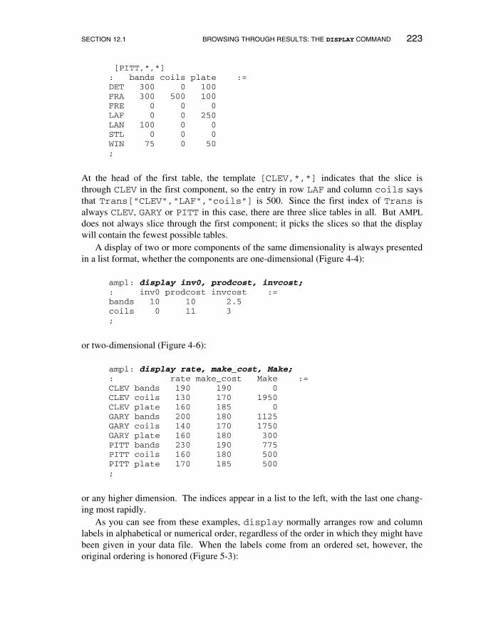
[PITT,*,*]: bands coils plate :=DET 300 0 100FRA 300 500 100FRE 0 0 0LAF 0 0 250LAN 100 0 0STL 0 0 0WIN 75 0 50;
At the head of the first table, the template [CLEV,*,*] indicates that the slice isthrough CLEV in the first component, so the entry in row LAF and column coils saysthat Trans["CLEV","LAF","coils"] is 500. Since the first index of Trans isalways CLEV, GARY or PITT in this case, there are three slice tables in all. But AMPLdoes not always slice through the first component; it picks the slices so that the displaywill contain the fewest possible tables.
A display of two or more components of the same dimensionality is always presentedin a list format, whether the components are one-dimensional (Figure 4-4):
ampl: display inv0, prodcost, invcost;: inv0 prodcost invcost :=bands 10 10 2.5coils 0 11 3;
or two-dimensional (Figure 4-6):
ampl: display rate, make_cost, Make;: rate make_cost Make :=CLEV bands 190 190 0CLEV coils 130 170 1950CLEV plate 160 185 0GARY bands 200 180 1125GARY coils 140 170 1750GARY plate 160 180 300PITT bands 230 190 775PITT coils 160 180 500PITT plate 170 185 500;
or any higher dimension. The indices appear in a list to the left, with the last one chang-ing most rapidly.
As you can see from these examples, display normally arranges row and columnlabels in alphabetical or numerical order, regardless of the order in which they might havebeen given in your data file. When the labels come from an ordered set, however, theoriginal ordering is honored (Figure 5-3):

224 DISPLAY COMMANDS CHAPTER 12
ampl: display avail;avail [*] :=27sep 4004oct 4011oct 3218oct 40;
For this reason, it can be worthwhile to declare certain sets of your model to be ordered,even if their ordering plays no explicit role in your formulation.
Displaying indexed expressions
The display command can show the value of any arithmetic expression that isvalid in an AMPL model. Single-valued expressions pose no difficulty, as in the case ofthese three profit components from Figure 4-4:
ampl: display sum {p in PROD,t in 1..T} revenue[p,t]*Sell[p,t],ampl? sum {p in PROD,t in 1..T} prodcost[p]*Make[p,t],ampl? sum {p in PROD,t in 1..T} invcost[p]*Inv[p,t];sum{p in PROD, t in 1 .. T} revenue[p,t]*Sell[p,t] = 787810sum{p in PROD, t in 1 .. T} prodcost[p]*Make[p,t] = 269477sum{p in PROD, t in 1 .. T} invcost[p]*Inv[p,t] = 3300
Suppose, however, that you want to see all the individual values of revenue[p,t] *Sell[p,t]. Since you can type display revenue, Sell to display the separatevalues of revenue[p,t] and Sell[p,t], you might want to ask for the products ofthese values by typing:
ampl: display revenue * Sell;syntax errorcontext: display revenue >>> * <<< Sell;
AMPL does not recognize this kind of array arithmetic. To display an indexed collectionof expressions, you must specify the indexing explicitly:
ampl: display {p in PROD, t in 1..T} revenue[p,t]*Sell[p,t];revenue[p,t]*Sell[p,t] [*,*] (tr): bands coils :=1 150000 92102 156000 875003 37800 1295004 54000 163800;
To apply the same indexing to two or more expressions, enclose a list of them in paren-theses after the indexing expression:

SECTION 12.1 BROWSING THROUGH RESULTS: THE DISPLAY COMMAND 225
ampl: display {p in PROD, t in 1..T}ampl? (revenue[p,t]*Sell[p,t], prodcost[p]*Make[p,t]);: revenue[p,t]*Sell[p,t] prodcost[p]*Make[p,t] :=bands 1 150000 59900bands 2 156000 60000bands 3 37800 14000bands 4 54000 20000coils 1 9210 15477coils 2 87500 15400coils 3 129500 38500coils 4 163800 46200;
An indexing expression followed by an expression or parenthesized list of expressions istreated as a single display item, which specifies some indexed collection of values. Adisplay command may contain one of these items as above, or a comma-separated listof them.
The presentation of the values for indexed expressions follows the same rules as forindividual parameters and variables. In fact, you can regard a command like
display revenue, Sell
as shorthand for
ampl: display {p in PROD, t in 1..T} (revenue[p,t],Sell[p,t]);: revenue[p,t] Sell[p,t] :=bands 1 25 6000bands 2 26 6000bands 3 27 1400bands 4 27 2000coils 1 30 307coils 2 35 2500coils 3 37 3500coils 4 39 4200;
If you rearrange the indexing expression so that t in 1..T comes first, however, therows of the list are instead sorted first on the members of 1..T:
ampl: display {t in 1..T, p in PROD} (revenue[p,t],Sell[p,t]);: revenue[p,t] Sell[p,t] :=1 bands 25 60001 coils 30 3072 bands 26 60002 coils 35 25003 bands 27 14003 coils 37 35004 bands 27 20004 coils 39 4200;
This change in the default presentation can only be achieved by placing an explicit index-ing expression after display.
226 DISPLAY COMMANDS CHAPTER 12
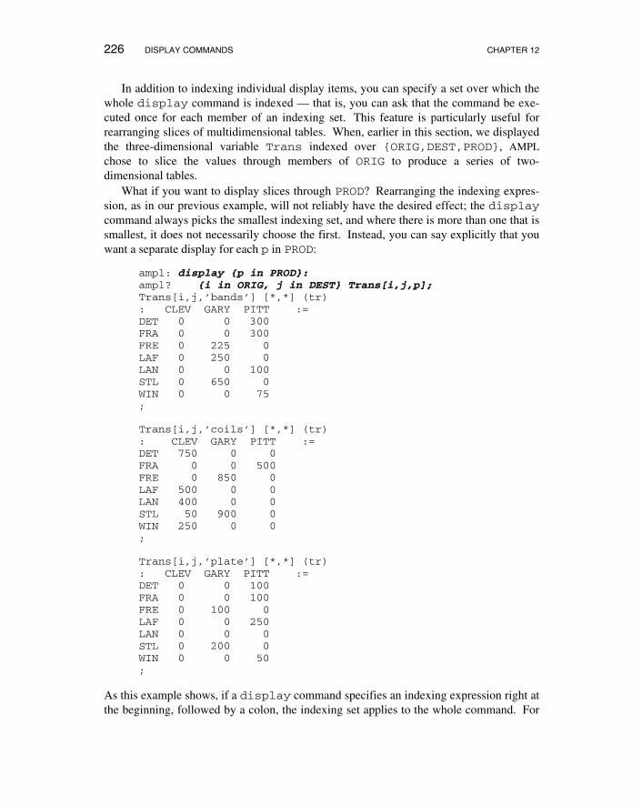
In addition to indexing individual display items, you can specify a set over which thewhole display command is indexed — that is, you can ask that the command be exe-cuted once for each member of an indexing set. This feature is particularly useful forrearranging slices of multidimensional tables. When, earlier in this section, we displayedthe three-dimensional variable Trans indexed over {ORIG,DEST,PROD}, AMPLchose to slice the values through members of ORIG to produce a series of two-dimensional tables.
What if you want to display slices through PROD? Rearranging the indexing expres-sion, as in our previous example, will not reliably have the desired effect; the displaycommand always picks the smallest indexing set, and where there is more than one that issmallest, it does not necessarily choose the first. Instead, you can say explicitly that youwant a separate display for each p in PROD:
ampl: display {p in PROD}:ampl? {i in ORIG, j in DEST} Trans[i,j,p];Trans[i,j,’bands’] [*,*] (tr): CLEV GARY PITT :=DET 0 0 300FRA 0 0 300FRE 0 225 0LAF 0 250 0LAN 0 0 100STL 0 650 0WIN 0 0 75;
Trans[i,j,’coils’] [*,*] (tr): CLEV GARY PITT :=DET 750 0 0FRA 0 0 500FRE 0 850 0LAF 500 0 0LAN 400 0 0STL 50 900 0WIN 250 0 0;
Trans[i,j,’plate’] [*,*] (tr): CLEV GARY PITT :=DET 0 0 100FRA 0 0 100FRE 0 100 0LAF 0 0 250LAN 0 0 0STL 0 200 0WIN 0 0 50;
As this example shows, if a display command specifies an indexing expression right atthe beginning, followed by a colon, the indexing set applies to the whole command. For

SECTION 12.2 FORMATTING OPTIONS FOR DISPLAY 227
____________________________________________________________________________________________________________________________________________________________________________________________________________________________________________________________
display_1col maximum elements for a table to be displayed in list format (20)display_transpose transpose tables if rows – columns < display_transpose (0)display_width maximum line width (79)gutter_width separation between table columns (3)omit_zero_cols if not 0, omit all-zero columns from displays (0)omit_zero_rows if not 0, omit all-zero rows from displays (0)
Table 12-1: Formatting options for display (with default values).____________________________________________________________________________________________________________________________________________________________________________________________________________________________________________________________
each member of the set, the expressions following the colon are evaluated and displayedseparately.
12.2 Formatting options for display
The display command uses a few simple rules for choosing a good arrangement ofdata. By changing several options, you can control overall arrangement, handling of zerovalues, and line width. These options are summarized in Table 12-1, with default valuesshown in parentheses.
Arrangement of lists and tables
The display of a one-dimensional parameter or variable can produce a very long list,as in this example from the scheduling model of Figure 16-5:
ampl: display required;required [*] :=Fri1 100Fri2 78Fri3 52Mon1 100Mon2 78Mon3 52Sat1 100Sat2 78Thu1 100Thu2 78Thu3 52Tue1 100Tue2 78Tue3 52Wed1 100Wed2 78Wed3 52;
228 DISPLAY COMMANDS CHAPTER 12
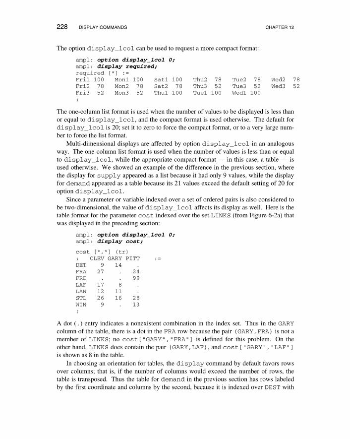
The option display_1col can be used to request a more compact format:
ampl: option display_1col 0;ampl: display required;required [*] :=Fri1 100 Mon1 100 Sat1 100 Thu2 78 Tue2 78 Wed2 78Fri2 78 Mon2 78 Sat2 78 Thu3 52 Tue3 52 Wed3 52Fri3 52 Mon3 52 Thu1 100 Tue1 100 Wed1 100;
The one-column list format is used when the number of values to be displayed is less thanor equal to display_1col, and the compact format is used otherwise. The default fordisplay_1col is 20; set it to zero to force the compact format, or to a very large num-ber to force the list format.
Multi-dimensional displays are affected by option display_1col in an analogousway. The one-column list format is used when the number of values is less than or equalto display_1col, while the appropriate compact format — in this case, a table — isused otherwise. We showed an example of the difference in the previous section, wherethe display for supply appeared as a list because it had only 9 values, while the displayfor demand appeared as a table because its 21 values exceed the default setting of 20 foroption display_1col.
Since a parameter or variable indexed over a set of ordered pairs is also considered tobe two-dimensional, the value of display_1col affects its display as well. Here is thetable format for the parameter cost indexed over the set LINKS (from Figure 6-2a) thatwas displayed in the preceding section:
ampl: option display_1col 0;ampl: display cost;
cost [*,*] (tr): CLEV GARY PITT :=DET 9 14 .FRA 27 . 24FRE . . 99LAF 17 8 .LAN 12 11 .STL 26 16 28WIN 9 . 13;
A dot (.) entry indicates a nonexistent combination in the index set. Thus in the GARYcolumn of the table, there is a dot in the FRA row because the pair (GARY,FRA) is not amember of LINKS; no cost["GARY","FRA"] is defined for this problem. On theother hand, LINKS does contain the pair (GARY,LAF), and cost["GARY","LAF"]is shown as 8 in the table.
In choosing an orientation for tables, the display command by default favors rowsover columns; that is, if the number of columns would exceed the number of rows, thetable is transposed. Thus the table for demand in the previous section has rows labeledby the first coordinate and columns by the second, because it is indexed over DEST with
SECTION 12.2 FORMATTING OPTIONS FOR DISPLAY 229
7 members and then PROD with 3 members. By contrast, the table for cost has columnslabeled by the first coordinate and rows by the second, because it is indexed over ORIGwith 3 members and then DEST with 7 members. A transposed table is indicated by a(tr) in its first line.
The transposition status of a table can be reversed by changing thedisplay_transpose option. Positive values tend to force transposition:
ampl: option display_transpose 5;ampl: display demand;demand [*,*] (tr): DET FRA FRE LAF LAN STL WIN :=bands 300 300 225 250 100 650 75coils 750 500 850 500 400 950 250plate 100 100 100 250 0 200 50;
while negative values tend to suppress it:
ampl: option display_transpose -5;ampl: display cost;cost [*,*]: DET FRA FRE LAF LAN STL WIN :=CLEV 9 27 . 17 12 26 9GARY 14 . . 8 11 16 .PITT . 24 99 . . 28 13;
The rule is as follows: a table is transposed only when the number of rows minus thenumber of columns would be less than display_transpose. At its default value ofzero, display_transpose gives the previously described default behavior.
Control of line width
The option display_width gives the maximum number of characters on a linegenerated by display (as seen in the model of Figure 16-4):
ampl: option display_width 50, display_1col 0;ampl: display required;
required [*] :=Fri1 100 Mon3 52 Thu3 52 Wed2 78Fri2 78 Sat1 100 Tue1 100 Wed3 52Fri3 52 Sat2 78 Tue2 78Mon1 100 Thu1 100 Tue3 52Mon2 78 Thu2 78 Wed1 100;
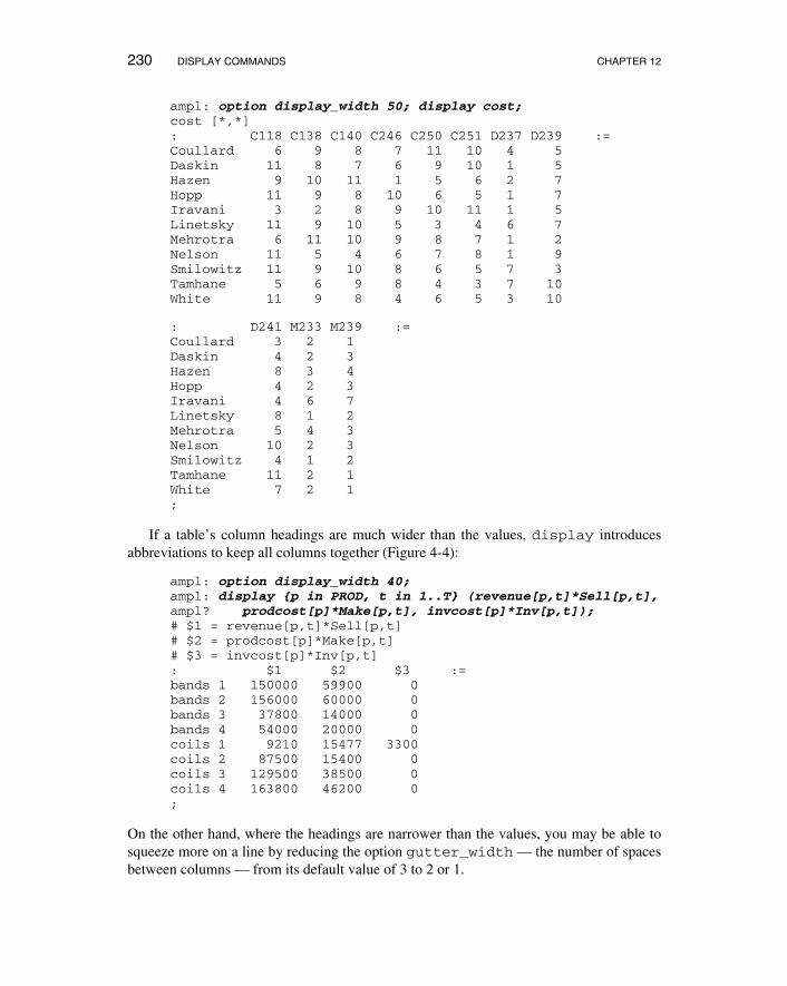
When a table would be wider than display_width, it is cut vertically into two ormore tables. The row names in each table are the same, but the columns are different:
230 DISPLAY COMMANDS CHAPTER 12
ampl: option display_width 50; display cost;cost [*,*]: C118 C138 C140 C246 C250 C251 D237 D239 :=Coullard 6 9 8 7 11 10 4 5Daskin 11 8 7 6 9 10 1 5Hazen 9 10 11 1 5 6 2 7Hopp 11 9 8 10 6 5 1 7Iravani 3 2 8 9 10 11 1 5Linetsky 11 9 10 5 3 4 6 7Mehrotra 6 11 10 9 8 7 1 2Nelson 11 5 4 6 7 8 1 9Smilowitz 11 9 10 8 6 5 7 3Tamhane 5 6 9 8 4 3 7 10White 11 9 8 4 6 5 3 10
: D241 M233 M239 :=Coullard 3 2 1Daskin 4 2 3Hazen 8 3 4Hopp 4 2 3Iravani 4 6 7Linetsky 8 1 2Mehrotra 5 4 3Nelson 10 2 3Smilowitz 4 1 2Tamhane 11 2 1White 7 2 1;
If a table’s column headings are much wider than the values, display introducesabbreviations to keep all columns together (Figure 4-4):
ampl: option display_width 40;ampl: display {p in PROD, t in 1..T} (revenue[p,t]*Sell[p,t],ampl? prodcost[p]*Make[p,t], invcost[p]*Inv[p,t]);# $1 = revenue[p,t]*Sell[p,t]# $2 = prodcost[p]*Make[p,t]# $3 = invcost[p]*Inv[p,t]: $1 $2 $3 :=bands 1 150000 59900 0bands 2 156000 60000 0bands 3 37800 14000 0bands 4 54000 20000 0coils 1 9210 15477 3300coils 2 87500 15400 0coils 3 129500 38500 0coils 4 163800 46200 0;
On the other hand, where the headings are narrower than the values, you may be able tosqueeze more on a line by reducing the option gutter_width — the number of spacesbetween columns — from its default value of 3 to 2 or 1.

SECTION 12.2 FORMATTING OPTIONS FOR DISPLAY 231
Suppression of zeros
In some kinds of linear programs that have many more variables than constraints,most of the variables have an optimal value of zero. For instance in the assignment prob-lem of Figure 3-2, the optimal values of all the variables form this table, in which there isa single 1 in each row and each column:
ampl: display Trans;
Trans [*,*]: C118 C138 C140 C246 C250 C251 D237 D239 D241 M233 M239 :=Coullard 1 0 0 0 0 0 0 0 0 0 0Daskin 0 0 0 0 0 0 0 0 1 0 0Hazen 0 0 0 1 0 0 0 0 0 0 0Hopp 0 0 0 0 0 0 1 0 0 0 0Iravani 0 1 0 0 0 0 0 0 0 0 0Linetsky 0 0 0 0 1 0 0 0 0 0 0Mehrotra 0 0 0 0 0 0 0 1 0 0 0Nelson 0 0 1 0 0 0 0 0 0 0 0Smilowitz 0 0 0 0 0 0 0 0 0 1 0Tamhane 0 0 0 0 0 1 0 0 0 0 0White 0 0 0 0 0 0 0 0 0 0 1;
By setting omit_zero_rows to 1, all the zero values are suppressed, and the listcomes down to the entries of interest:
ampl: option omit_zero_rows 1;
ampl: display Trans;
Trans :=Coullard C118 1Daskin D241 1Hazen C246 1Hopp D237 1Iravani C138 1Linetsky C250 1Mehrotra D239 1Nelson C140 1Smilowitz M233 1Tamhane C251 1White M239 1;
If the number of nonzero entries is less than the value of display_1col, the data isprinted as a list, as it is here. If the number of nonzeros is greater than display_1col,a table format would be used, and the omit_zero_rows option would only suppresstable rows that contain all zero entries.
For example, the display of the three-dimensional variable Trans from earlier in thischapter would be condensed to the following:
232 DISPLAY COMMANDS CHAPTER 12
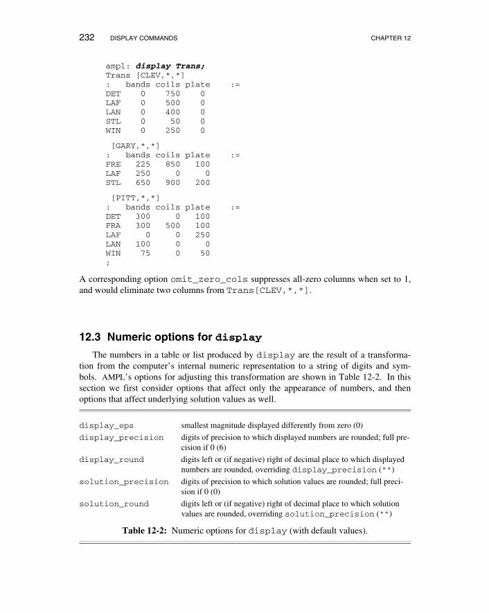
ampl: display Trans;Trans [CLEV,*,*]: bands coils plate :=DET 0 750 0LAF 0 500 0LAN 0 400 0STL 0 50 0WIN 0 250 0
[GARY,*,*]: bands coils plate :=FRE 225 850 100LAF 250 0 0STL 650 900 200
[PITT,*,*]: bands coils plate :=DET 300 0 100FRA 300 500 100LAF 0 0 250LAN 100 0 0WIN 75 0 50;
A corresponding option omit_zero_cols suppresses all-zero columns when set to 1,and would eliminate two columns from Trans[CLEV,*,*].
12.3 Numeric options for display
The numbers in a table or list produced by display are the result of a transforma-tion from the computer’s internal numeric representation to a string of digits and sym-bols. AMPL’s options for adjusting this transformation are shown in Table 12-2. In thissection we first consider options that affect only the appearance of numbers, and thenoptions that affect underlying solution values as well.____________________________________________________________________________________________________________________________________________________________________________________________________________________________________________________________
display_eps smallest magnitude displayed differently from zero (0)
display_precision digits of precision to which displayed numbers are rounded; full pre-cision if 0 (6)
display_round digits left or (if negative) right of decimal place to which displayednumbers are rounded, overriding display_precision ("")
solution_precision digits of precision to which solution values are rounded; full preci-sion if 0 (0)
solution_round digits left or (if negative) right of decimal place to which solutionvalues are rounded, overriding solution_precision ("")
Table 12-2: Numeric options for display (with default values).____________________________________________________________________________________________________________________________________________________________________________________________________________________________________________________________
SECTION 12.3 NUMERIC OPTIONS FOR DISPLAY 233
Appearance of numeric values
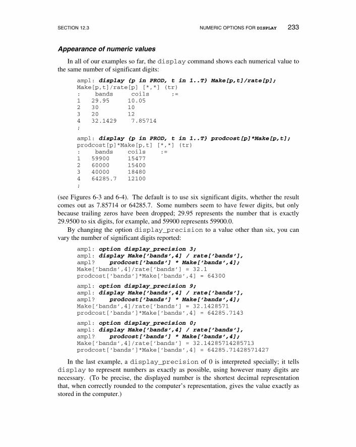
In all of our examples so far, the display command shows each numerical value tothe same number of significant digits:
ampl: display {p in PROD, t in 1..T} Make[p,t]/rate[p];Make[p,t]/rate[p] [*,*] (tr): bands coils :=1 29.95 10.052 30 103 20 124 32.1429 7.85714;
ampl: display {p in PROD, t in 1..T} prodcost[p]*Make[p,t];prodcost[p]*Make[p,t] [*,*] (tr): bands coils :=1 59900 154772 60000 154003 40000 184804 64285.7 12100;
(see Figures 6-3 and 6-4). The default is to use six significant digits, whether the resultcomes out as 7.85714 or 64285.7. Some numbers seem to have fewer digits, but onlybecause trailing zeros have been dropped; 29.95 represents the number that is exactly29.9500 to six digits, for example, and 59900 represents 59900.0.
By changing the option display_precision to a value other than six, you canvary the number of significant digits reported:
ampl: option display_precision 3;ampl: display Make[’bands’,4] / rate[’bands’],ampl? prodcost[’bands’] * Make[’bands’,4];Make[’bands’,4]/rate[’bands’] = 32.1prodcost[’bands’]*Make[’bands’,4] = 64300
ampl: option display_precision 9;ampl: display Make[’bands’,4] / rate[’bands’],ampl? prodcost[’bands’] * Make[’bands’,4];Make[’bands’,4]/rate[’bands’] = 32.1428571prodcost[’bands’]*Make[’bands’,4] = 64285.7143
ampl: option display_precision 0;ampl: display Make[’bands’,4] / rate[’bands’],ampl? prodcost[’bands’] * Make[’bands’,4];Make[’bands’,4]/rate[’bands’] = 32.14285714285713prodcost[’bands’]*Make[’bands’,4] = 64285.71428571427
In the last example, a display_precision of 0 is interpreted specially; it tellsdisplay to represent numbers as exactly as possible, using however many digits arenecessary. (To be precise, the displayed number is the shortest decimal representationthat, when correctly rounded to the computer’s representation, gives the value exactly asstored in the computer.)

234 DISPLAY COMMANDS CHAPTER 12
Displays to a given precision provide the same degree of useful information abouteach number, but they can look ragged due to the varying numbers of digits after the dec-imal point. To specify rounding to a fixed number of decimal places, regardless of theresulting precision, you may set the option display_round. A nonnegative valuespecifies the number of digits to appear after the decimal point:
ampl: option display_round 2;ampl: display {p in PROD, t in 1..T} Make[p,t]/rate[p];Make[p,t]/rate[p] [*,*] (tr): bands coils :=1 29.95 10.052 30.00 10.003 20.00 12.004 32.14 7.86;
A negative value indicates rounding before the decimal point. For example, whendisplay_round is –2, all numbers are rounded to hundreds:
ampl: option display_round -2;ampl: display {p in PROD, t in 1..T} prodcost[p]*Make[p,t];prodcost[p]*Make[p,t] [*,*] (tr): bands coils :=1 59900 155002 60000 154003 40000 185004 64300 12100;
Any integer value of display_round overrides the effect of display_precision.To turn off display_round, set it to some non-integer such as the empty string ’’.
Depending on the solver you employ, you may find that some of the solution valuesthat ought to be zero do not always quite come out that way. For example, here is onesolver’s report of the objective function terms cost[i,j] * Trans[i,j] for theassignment problem of Section 3.3:
ampl: option omit_zero_rows 1;ampl: display {i in ORIG, j in DEST} cost[i,j] * Trans[i,j];cost[i,j]*Trans[i,j] :=Coullard C118 6Coullard D241 2.05994e-17Daskin D237 1Hazen C246 1Hopp D237 6.86647e-18Hopp D241 4... 9 lines omittedWhite C246 2.74659e-17White C251 -3.43323e-17White M239 1;
SECTION 12.3 NUMERIC OPTIONS FOR DISPLAY 235
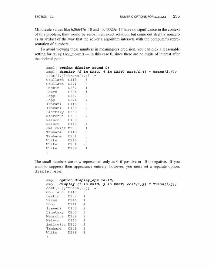
Minuscule values like 6.86647e–18 and –3.43323e–17 have no significance in the contextof this problem; they would be zeros in an exact solution, but come out slightly nonzeroas an artifact of the way that the solver’s algorithm interacts with the computer’s repre-sentation of numbers.
To avoid viewing these numbers in meaningless precision, you can pick a reasonablesetting for display_round — in this case 0, since there are no digits of interest afterthe decimal point:
ampl: option display_round 0;ampl: display {i in ORIG, j in DEST} cost[i,j] * Trans[i,j];cost[i,j]*Trans[i,j] :=Coullard C118 6Coullard D241 0Daskin D237 1Hazen C246 1Hopp D237 0Hopp D241 4Iravani C118 0Iravani C138 2Linetsky C250 3Mehrotra D239 2Nelson C138 0Nelson C140 4Smilowitz M233 1Tamhane C118 -0Tamhane C251 3White C246 0White C251 -0White M239 1;
The small numbers are now represented only as 0 if positive or –0 if negative. If youwant to suppress their appearance entirely, however, you must set a separate option,display_eps:
ampl: option display_eps 1e-10;ampl: display {i in ORIG, j in DEST} cost[i,j] * Trans[i,j];cost[i,j]*Trans[i,j] :=Coullard C118 6Daskin D237 1Hazen C246 1Hopp D241 4Iravani C138 2Linetsky C250 3Mehrotra D239 2Nelson C140 4Smilowitz M233 1Tamhane C251 3White M239 1;
236 DISPLAY COMMANDS CHAPTER 12
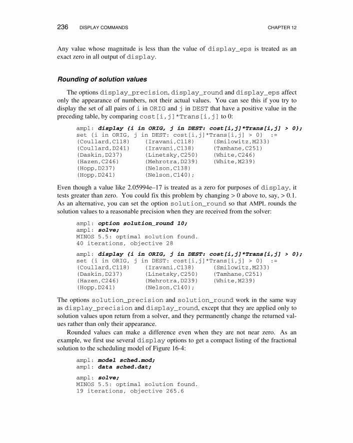
Any value whose magnitude is less than the value of display_eps is treated as anexact zero in all output of display.
Rounding of solution values
The options display_precision, display_round and display_eps affectonly the appearance of numbers, not their actual values. You can see this if you try todisplay the set of all pairs of i in ORIG and j in DEST that have a positive value in thepreceding table, by comparing cost[i,j]*Trans[i,j] to 0:
ampl: display {i in ORIG, j in DEST: cost[i,j]*Trans[i,j] > 0};set {i in ORIG, j in DEST: cost[i,j]*Trans[i,j] > 0} :=(Coullard,C118) (Iravani,C118) (Smilowitz,M233)(Coullard,D241) (Iravani,C138) (Tamhane,C251)(Daskin,D237) (Linetsky,C250) (White,C246)(Hazen,C246) (Mehrotra,D239) (White,M239)(Hopp,D237) (Nelson,C138)(Hopp,D241) (Nelson,C140);
Even though a value like 2.05994e–17 is treated as a zero for purposes of display, ittests greater than zero. You could fix this problem by changing > 0 above to, say, > 0.1.As an alternative, you can set the option solution_round so that AMPL rounds thesolution values to a reasonable precision when they are received from the solver:
ampl: option solution_round 10;ampl: solve;MINOS 5.5: optimal solution found.40 iterations, objective 28
ampl: display {i in ORIG, j in DEST: cost[i,j]*Trans[i,j] > 0};set {i in ORIG, j in DEST: cost[i,j]*Trans[i,j] > 0} :=(Coullard,C118) (Iravani,C138) (Smilowitz,M233)(Daskin,D237) (Linetsky,C250) (Tamhane,C251)(Hazen,C246) (Mehrotra,D239) (White,M239)(Hopp,D241) (Nelson,C140);
The options solution_precision and solution_round work in the same wayas display_precision and display_round, except that they are applied only tosolution values upon return from a solver, and they permanently change the returned val-ues rather than only their appearance.
Rounded values can make a difference even when they are not near zero. As anexample, we first use several display options to get a compact listing of the fractionalsolution to the scheduling model of Figure 16-4:
ampl: model sched.mod;ampl: data sched.dat;
ampl: solve;MINOS 5.5: optimal solution found.19 iterations, objective 265.6

SECTION 12.3 NUMERIC OPTIONS FOR DISPLAY 237
ampl: option display_width 60;ampl: option display_1col 5;
ampl: option display_eps 1e-10;ampl: option omit_zero_rows 1;ampl: display Work;Work [*] :=10 28.8 30 14.4 71 35.6 106 23.2 123 35.618 7.6 35 6.8 73 28 109 14.424 6.8 66 35.6 87 14.4 113 14.4;
Each value Work[j] represents the number of workers assigned to schedule j. We canget a quick practical schedule by rounding the fractional values up to the next highestinteger; using the ceil function to perform the rounding, we see that the total number ofworkers needed should be:
ampl: display sum {j in SCHEDS} ceil(Work[j]);sum{j in SCHEDS} ceil(Work[j]) = 273
If we copy the numbers from the preceding table and round them up by hand, however,we find that they only sum to 271. The source of the difficulty can be seen by displayingthe numbers to full precision:
ampl: option display_eps 0;ampl: option display_precision 0;
ampl: display Work;Work [*] :=10 28.799999999999997 73 28.00000000000001818 7.599999999999998 87 14.39999999999999524 6.79999999999999 95 -5.876671973951407e-1530 14.40000000000001 106 23.20000000000000635 6.799999999999995 108 4.685288280240683e-1655 -4.939614313857677e-15 109 14.466 35.6 113 14.471 35.599999999999994 123 35.59999999999999;
Half the problem is due to the minuscule positive value of Work[108], which wasrounded up to 1. The other half is due to Work[73]; although it is 28 in an exact solu-tion, it comes back from the solver with a slightly larger value of 28.000000000000018,so it gets rounded up to 29.
The easiest way to ensure that our arithmetic works correctly in this case is again toset solution_round before solve:
ampl: option solution_round 10;ampl: solve;MINOS 5.5: optimal solution found.19 iterations, objective 265.6
ampl: display sum {j in SCHEDS} ceil(Work[j]);sum{j in SCHEDS} ceil(Work[j]) = 271
238 DISPLAY COMMANDS CHAPTER 12
We picked a value of 10 for solution_round because we observed that the slightinaccuracies in the solver’s values occurred well past the 10th decimal place.
The effect of solution_round or solution_precision applies to all valuesreturned by the solver. To modify only certain values, use the assignment (let) com-mand described in Section 11.3 together with the rounding functions in Table 11-1.
12.4 Other output commands: print and printf
Two additional AMPL commands have much the same syntax as display, but donot automatically format their output. The print command does no formatting at all,while the printf command requires an explicit description of the desired formatting.
The print command
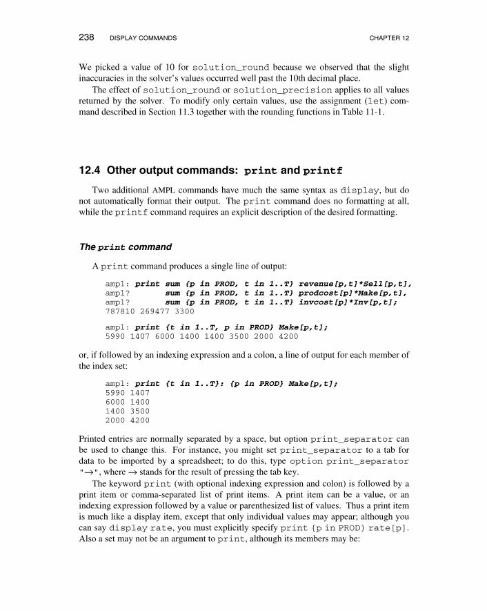
A print command produces a single line of output:
ampl: print sum {p in PROD, t in 1..T} revenue[p,t]*Sell[p,t],ampl? sum {p in PROD, t in 1..T} prodcost[p]*Make[p,t],ampl? sum {p in PROD, t in 1..T} invcost[p]*Inv[p,t];787810 269477 3300
ampl: print {t in 1..T, p in PROD} Make[p,t];5990 1407 6000 1400 1400 3500 2000 4200
or, if followed by an indexing expression and a colon, a line of output for each member ofthe index set:
ampl: print {t in 1..T}: {p in PROD} Make[p,t];5990 14076000 14001400 35002000 4200
Printed entries are normally separated by a space, but option print_separator canbe used to change this. For instance, you might set print_separator to a tab fordata to be imported by a spreadsheet; to do this, type option print_separator"→", where → stands for the result of pressing the tab key.
The keyword print (with optional indexing expression and colon) is followed by aprint item or comma-separated list of print items. A print item can be a value, or anindexing expression followed by a value or parenthesized list of values. Thus a print itemis much like a display item, except that only individual values may appear; although youcan say display rate, you must explicitly specify print {p in PROD} rate[p].Also a set may not be an argument to print, although its members may be:
SECTION 12.4 OTHER OUTPUT COMMANDS: PRINT AND PRINTF 239
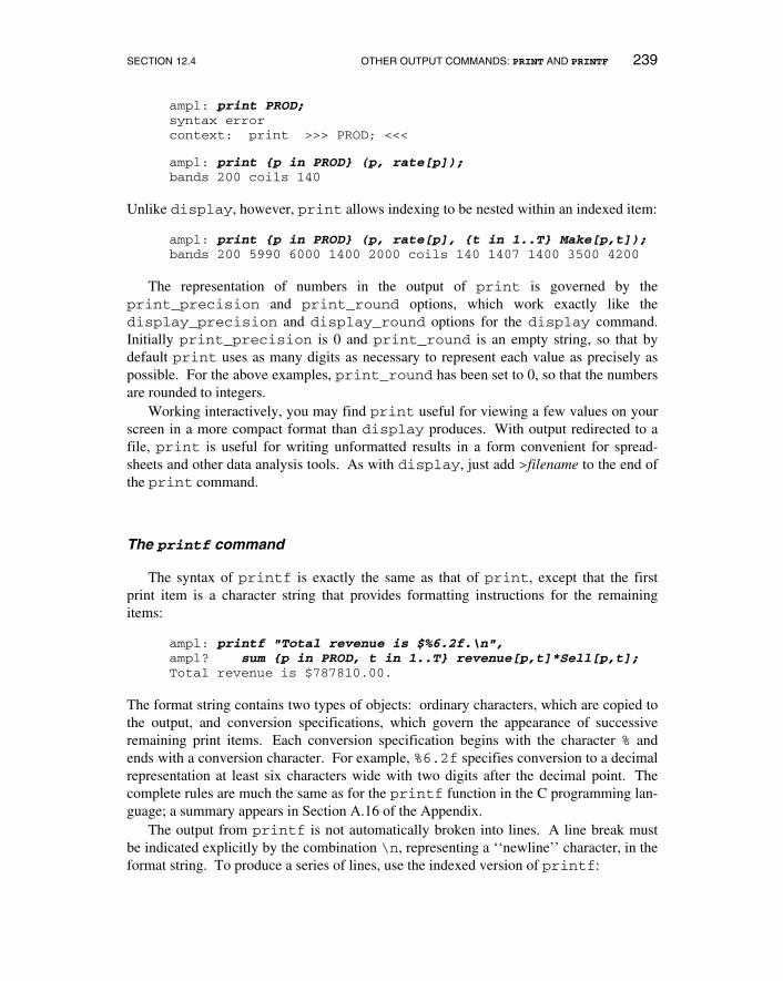
ampl: print PROD;syntax errorcontext: print >>> PROD; <<<
ampl: print {p in PROD} (p, rate[p]);bands 200 coils 140
Unlike display, however, print allows indexing to be nested within an indexed item:
ampl: print {p in PROD} (p, rate[p], {t in 1..T} Make[p,t]);bands 200 5990 6000 1400 2000 coils 140 1407 1400 3500 4200
The representation of numbers in the output of print is governed by theprint_precision and print_round options, which work exactly like thedisplay_precision and display_round options for the display command.Initially print_precision is 0 and print_round is an empty string, so that bydefault print uses as many digits as necessary to represent each value as precisely aspossible. For the above examples, print_round has been set to 0, so that the numbersare rounded to integers.
Working interactively, you may find print useful for viewing a few values on yourscreen in a more compact format than display produces. With output redirected to afile, print is useful for writing unformatted results in a form convenient for spread-sheets and other data analysis tools. As with display, just add >filename to the end ofthe print command.
The printf command
The syntax of printf is exactly the same as that of print, except that the firstprint item is a character string that provides formatting instructions for the remainingitems:
ampl: printf "Total revenue is $%6.2f.\n",ampl? sum {p in PROD, t in 1..T} revenue[p,t]*Sell[p,t];Total revenue is $787810.00.
The format string contains two types of objects: ordinary characters, which are copied tothe output, and conversion specifications, which govern the appearance of successiveremaining print items. Each conversion specification begins with the character % andends with a conversion character. For example, %6.2f specifies conversion to a decimalrepresentation at least six characters wide with two digits after the decimal point. Thecomplete rules are much the same as for the printf function in the C programming lan-guage; a summary appears in Section A.16 of the Appendix.
The output from printf is not automatically broken into lines. A line break mustbe indicated explicitly by the combination \n, representing a ‘‘newline’’ character, in theformat string. To produce a series of lines, use the indexed version of printf:

240 DISPLAY COMMANDS CHAPTER 12
ampl: printf {t in 1..T}: "%3i%12.2f%12.2f\n", t,ampl? sum {p in PROD} revenue[p,t]*Sell[p,t],ampl? sum {p in PROD} prodcost[p]*Make[p,t];
1 159210.00 75377.002 243500.00 75400.003 167300.00 52500.004 217800.00 66200.00
This printf is executed once for each member of the indexing set preceding the colon;for each t in 1..T the format is applied again, and the \n character generates anotherline break.
The printf command is mainly useful, in conjunction with redirection of output toa file, for printing short summary reports in a readable format. Because the number ofconversion specifications in the format string must match the number of values beingprinted, printf cannot conveniently produce tables in which the number of items on aline may vary from run to run, such as a table of all Make[p,t] values.
12.5 Related solution values
Sets, parameters and variables are the most obvious things to look at in interpretingthe solution of a linear program, but AMPL also provides ways of examining objectives,bounds, slacks, dual prices and reduced costs associated with the optimal solution.
As we have shown in numerous examples already, AMPL distinguishes the variousvalues associated with a model component by use of ‘‘qualified’’ names that consist of avariable or constraint identifier, a dot (.), and a predefined ‘‘suffix’’ string. For instance,the upper bounds for the variable Make are called Make.ub, and the upper bound forMake["coils",2] is written Make["coils",2].ub. (Note that the suffix comesafter the subscript.) A qualified name can be used like an unqualified one, so thatdisplay Make.ub prints a table of upper bounds on the Make variables, whiledisplay Make, Make.ub prints a list of the optimal values and upper bounds.
Objective functions
The name of the objective function (from a minimize or maximize declaration)refers to the objective’s value computed from the current values of the variables. Thisname can be used to represent the optimal objective value in display, print, orprintf:
ampl: print 100 * Total_Profit /ampl? sum {p in PROD, t in 1..T} revenue[p,t] * Sell[p,t];65.37528084182735
If the current model declares several objective functions, you can refer to any of them,even though only one has been optimized.
SECTION 12.5 RELATED SOLUTION VALUES 241
Bounds and slacks
The suffixes .lb and .ub on a variable denote its lower and upper bounds, while.slack denotes the difference of a variable’s value from its nearer bound. Here’s anexample from Figure 5-1:
ampl: display Buy.lb, Buy, Buy.ub, Buy.slack;: Buy.lb Buy Buy.ub Buy.slack :=BEEF 2 2 10 0CHK 2 10 10 0FISH 2 2 10 0HAM 2 2 10 0MCH 2 2 10 0MTL 2 6.23596 10 3.76404SPG 2 5.25843 10 3.25843TUR 2 2 10 0;
The reported bounds are those that were sent to the solver. Thus they include not only thebounds specified in >= and <= phrases of var declarations, but also certain bounds thatwere deduced from the constraints by AMPL’s presolve phase. Other suffixes let youlook at the original bounds and at additional bounds deduced by presolve; see the discus-sion of presolve in Section 14.1 for details.
Two equal bounds denote a fixed variable, which is normally eliminated by presolve.Thus in the planning model of Figure 4-4, the constraint Inv[p,0] = inv0[p] fixesthe initial inventories:
ampl: display {p in PROD} (Inv[p,0].lb,inv0[p],Inv[p,0].ub);: Inv[p,0].lb inv0[p] Inv[p,0].ub :=bands 10 10 10coils 0 0 0;
In the production-and-transportation model of Figure 4-6, the constraint
sum {i in ORIG} Trans[i,j,p] = demand[j,p]
leads presolve to fix three variables at zero, because demand["LAN","plate"] iszero:
ampl: display {i in ORIG}ampl? (Trans[i,"LAN","plate"].lb,Trans[i,"LAN","plate"].ub);: Trans[i,’LAN’,’plate’].lb Trans[i,’LAN’,’plate’].ub :=CLEV 0 0GARY 0 0PITT 0 0;
As this example suggests, presolve’s adjustments to the bounds may depend on the dataas well as the structure of the constraints.
The concepts of bounds and slacks have an analogous interpretation for the con-straints of a model. Any AMPL constraint can be put into the standard form
242 DISPLAY COMMANDS CHAPTER 12
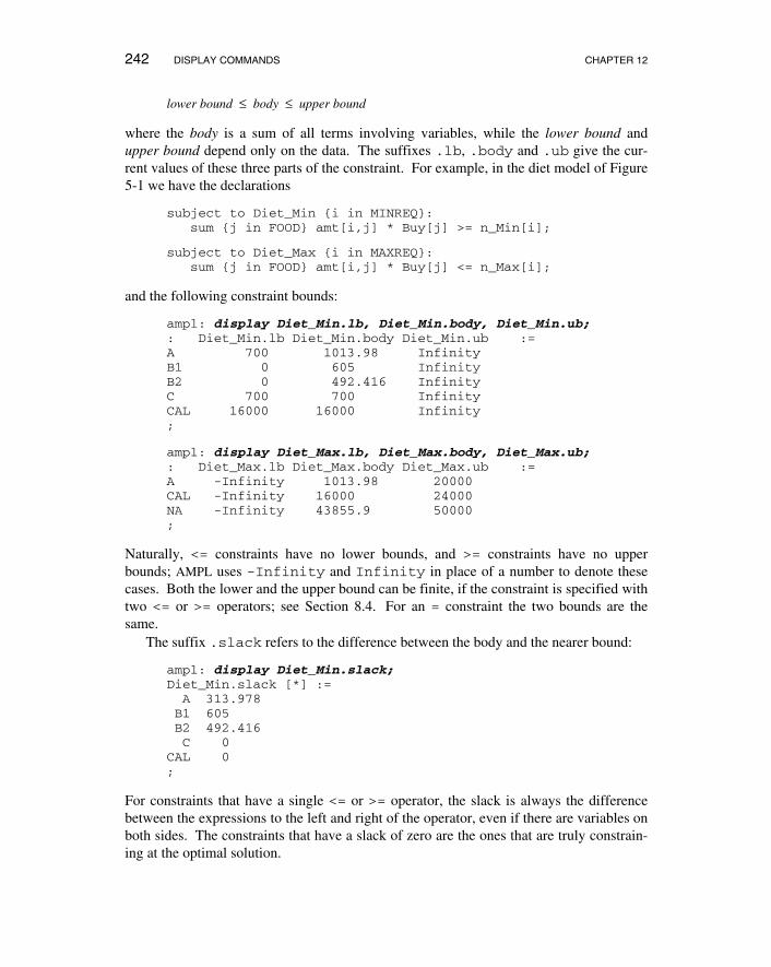
lower bound ≤ body ≤ upper bound
where the body is a sum of all terms involving variables, while the lower bound andupper bound depend only on the data. The suffixes .lb, .body and .ub give the cur-rent values of these three parts of the constraint. For example, in the diet model of Figure5-1 we have the declarations
subject to Diet_Min {i in MINREQ}:sum {j in FOOD} amt[i,j] * Buy[j] >= n_Min[i];
subject to Diet_Max {i in MAXREQ}:sum {j in FOOD} amt[i,j] * Buy[j] <= n_Max[i];
and the following constraint bounds:
ampl: display Diet_Min.lb, Diet_Min.body, Diet_Min.ub;: Diet_Min.lb Diet_Min.body Diet_Min.ub :=A 700 1013.98 InfinityB1 0 605 InfinityB2 0 492.416 InfinityC 700 700 InfinityCAL 16000 16000 Infinity;
ampl: display Diet_Max.lb, Diet_Max.body, Diet_Max.ub;: Diet_Max.lb Diet_Max.body Diet_Max.ub :=A -Infinity 1013.98 20000CAL -Infinity 16000 24000NA -Infinity 43855.9 50000;
Naturally, <= constraints have no lower bounds, and >= constraints have no upperbounds; AMPL uses -Infinity and Infinity in place of a number to denote thesecases. Both the lower and the upper bound can be finite, if the constraint is specified withtwo <= or >= operators; see Section 8.4. For an = constraint the two bounds are thesame.
The suffix .slack refers to the difference between the body and the nearer bound:
ampl: display Diet_Min.slack;Diet_Min.slack [*] :=
A 313.978B1 605B2 492.416C 0
CAL 0;
For constraints that have a single <= or >= operator, the slack is always the differencebetween the expressions to the left and right of the operator, even if there are variables onboth sides. The constraints that have a slack of zero are the ones that are truly constrain-ing at the optimal solution.

SECTION 12.5 RELATED SOLUTION VALUES 243
Dual values and reduced costs
Associated with each constraint in a linear program is a quantity variously known asthe dual variable, marginal value or shadow price. In the AMPL command environment,these dual values are denoted by the names of the constraints, without any qualifying suf-fix. Thus for example in Figure 4-6 there is a collection of constraints named Demand:
subject to Demand {j in DEST, p in PROD}:sum {i in ORIG} Trans[i,j,p] = demand[j,p];
and a table of the dual values associated with these constraints can be viewed by
ampl: display Demand;Demand [*,*]: bands coils plate :=DET 201 190.714 199FRA 209 204 211FRE 266.2 273.714 285LAF 201.2 198.714 205LAN 202 193.714 0STL 206.2 207.714 216WIN 200 190.714 198;
Solvers return optimal dual values to AMPL along with the optimal values of the ‘‘pri-mal’’ variables. We have space here only to summarize the most common interpretationof dual values; the extensive theory of duality and applications of dual variables can befound in any textbook on linear programming.
To start with an example, consider the constraint Demand["DET","bands"]above. If we change the value of the parameter demand["DET","bands"] in thisconstraint, the optimal value of the objective function Total_Cost changes accord-ingly. If we were to plot the optimal value of Total_Cost versus all possible values ofdemand["DET","bands"], the result would be a cost ‘‘curve’’ that shows how over-all cost varies with demand for bands at Detroit.
Additional computation would be necessary to determine the entire cost curve, butyou can learn something about it from the optimal dual values. After you solve the linearprogram using a particular value of demand["DET","bands"], the dual price for theconstraint tells you the slope of the cost curve, at the demand’s current value. In ourexample, reading from the table above, we find that the slope of the curve at the currentdemand is 201. This means that total production and shipping cost is increasing at therate of $201 for each extra ton of bands demanded at DET, or is decreasing by $201 foreach reduction of one ton in the demand.
As an example of an inequality, consider the following constraint from the samemodel:
subject to Time {i in ORIG}:sum {p in PROD} (1/rate[i,p]) * Make[i,p] <= avail[i];
244 DISPLAY COMMANDS CHAPTER 12
____________________________________________________________________________________________________________________________________________________________________________________________________________________________________________________________
constant term
optimalobjective
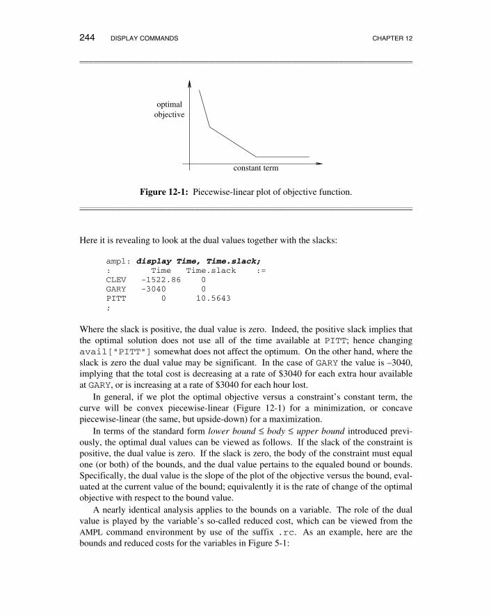
Figure 12-1: Piecewise-linear plot of objective function.____________________________________________________________________________________________________________________________________________________________________________________________________________________________________________________________
Here it is revealing to look at the dual values together with the slacks:
ampl: display Time, Time.slack;: Time Time.slack :=CLEV -1522.86 0GARY -3040 0PITT 0 10.5643;
Where the slack is positive, the dual value is zero. Indeed, the positive slack implies thatthe optimal solution does not use all of the time available at PITT; hence changingavail["PITT"] somewhat does not affect the optimum. On the other hand, where theslack is zero the dual value may be significant. In the case of GARY the value is –3040,implying that the total cost is decreasing at a rate of $3040 for each extra hour availableat GARY, or is increasing at a rate of $3040 for each hour lost.
In general, if we plot the optimal objective versus a constraint’s constant term, thecurve will be convex piecewise-linear (Figure 12-1) for a minimization, or concavepiecewise-linear (the same, but upside-down) for a maximization.
In terms of the standard form lower bound ≤ body ≤ upper bound introduced previ-ously, the optimal dual values can be viewed as follows. If the slack of the constraint ispositive, the dual value is zero. If the slack is zero, the body of the constraint must equalone (or both) of the bounds, and the dual value pertains to the equaled bound or bounds.Specifically, the dual value is the slope of the plot of the objective versus the bound, eval-uated at the current value of the bound; equivalently it is the rate of change of the optimalobjective with respect to the bound value.
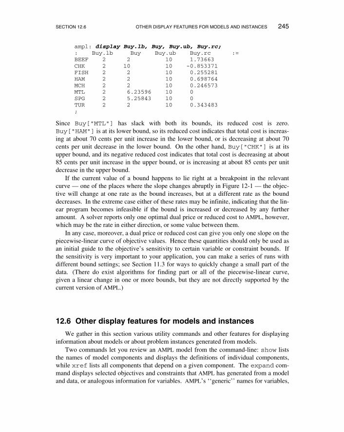
A nearly identical analysis applies to the bounds on a variable. The role of the dualvalue is played by the variable’s so-called reduced cost, which can be viewed from theAMPL command environment by use of the suffix .rc. As an example, here are thebounds and reduced costs for the variables in Figure 5-1:
SECTION 12.6 OTHER DISPLAY FEATURES FOR MODELS AND INSTANCES 245
ampl: display Buy.lb, Buy, Buy.ub, Buy.rc;: Buy.lb Buy Buy.ub Buy.rc :=BEEF 2 2 10 1.73663CHK 2 10 10 -0.853371FISH 2 2 10 0.255281HAM 2 2 10 0.698764MCH 2 2 10 0.246573MTL 2 6.23596 10 0SPG 2 5.25843 10 0TUR 2 2 10 0.343483;
Since Buy["MTL"] has slack with both its bounds, its reduced cost is zero.Buy["HAM"] is at its lower bound, so its reduced cost indicates that total cost is increas-ing at about 70 cents per unit increase in the lower bound, or is decreasing at about 70cents per unit decrease in the lower bound. On the other hand, Buy["CHK"] is at itsupper bound, and its negative reduced cost indicates that total cost is decreasing at about85 cents per unit increase in the upper bound, or is increasing at about 85 cents per unitdecrease in the upper bound.
If the current value of a bound happens to lie right at a breakpoint in the relevantcurve — one of the places where the slope changes abruptly in Figure 12-1 — the objec-tive will change at one rate as the bound increases, but at a different rate as the bounddecreases. In the extreme case either of these rates may be infinite, indicating that the lin-ear program becomes infeasible if the bound is increased or decreased by any furtheramount. A solver reports only one optimal dual price or reduced cost to AMPL, however,which may be the rate in either direction, or some value between them.
In any case, moreover, a dual price or reduced cost can give you only one slope on thepiecewise-linear curve of objective values. Hence these quantities should only be used asan initial guide to the objective’s sensitivity to certain variable or constraint bounds. Ifthe sensitivity is very important to your application, you can make a series of runs withdifferent bound settings; see Section 11.3 for ways to quickly change a small part of thedata. (There do exist algorithms for finding part or all of the piecewise-linear curve,given a linear change in one or more bounds, but they are not directly supported by thecurrent version of AMPL.)
12.6 Other display features for models and instances
We gather in this section various utility commands and other features for displayinginformation about models or about problem instances generated from models.
Two commands let you review an AMPL model from the command-line: show liststhe names of model components and displays the definitions of individual components,while xref lists all components that depend on a given component. The expand com-mand displays selected objectives and constraints that AMPL has generated from a modeland data, or analogous information for variables. AMPL’s ‘‘generic’’ names for variables,

246 DISPLAY COMMANDS CHAPTER 12
constraints, or objectives permit listings or tests that apply to all variables, constraints, orobjectives.
Displaying model components: the show command:
By itself, the show command lists the names of all components of the current model:
ampl: model multmip3.mod;ampl: show;parameters: demand fcost limit maxserve minload supply vcostsets: DEST ORIG PRODvariables: Trans Useconstraints: Demand Max_Serve Min_Ship Multi Supplyobjective: Total_Costchecks: one, called check 1.
This display may be restricted to components of one or more types:
ampl: show vars;variables: Trans Useampl: show obj, constr;objective: Total_Costconstraints: Demand Max_Serve Min_Ship Multi Supply
The show command can also display the declarations of individual components, savingyou the trouble of looking them up in the model file:
ampl: show Total_Cost;minimize Total_Cost: sum{i in ORIG, j in DEST, p in PROD}vcost[i,j,p]*Trans[i,j,p] + sum{i in ORIG, j in DEST}fcost[i,j]*Use[i,j];ampl: show vcost, fcost, Trans;param vcost{ORIG, DEST, PROD} >= 0;param fcost{ORIG, DEST} >= 0;var Trans{ORIG, DEST, PROD} >= 0;
If an item following show is the name of a component in the current model, the declara-tion of that component is displayed. Otherwise, the item is interpreted as a componenttype according to its first letter or two; see Section A.19.1. (Displayed declarations maydiffer in inessential ways from their appearance in your model file, due to transformationsthat AMPL performs when the model is parsed and translated.)
Since the check statements in a model do not have names, AMPL numbers them inthe order that they appear. Thus to see the third check statement you would type
ampl: show check 3;check{p in PROD} :
sum{i in ORIG} supply[i,p] == sum{j in DEST} demand[j,p];
By itself, show checks indicates the number of check statements in the model.

SECTION 12.6 OTHER DISPLAY FEATURES FOR MODELS AND INSTANCES 247
Displaying model dependencies: the xref command
The xref command lists all model components that depend on a specified compo-nent, either directly (by referring to it) or indirectly (by referring to its dependents). Ifmore than one component is given, the dependents are listed separately for each. Here isan example from multmip3.mod:
ampl: xref demand, Trans;# 2 entities depend on demand:check 1Demand# 5 entities depend on Trans:Total_CostSupplyDemandMultiMin_Ship
In general, the command is simply the keyword xref followed by a comma-separatedlist of any combination of set, parameter, variable, objective and constraint names.
Displaying model instances: the expand command
In checking a model and its data for correctness, you may want to look at some of thespecific constraints that AMPL is generating. The expand command displays all con-straints in a given indexed collection or specific constraints that you identify:
ampl: model nltrans.mod;ampl: data nltrans.dat;ampl: expand Supply;subject to Supply[’GARY’]:
Trans[’GARY’,’FRA’] + Trans[’GARY’,’DET’] +Trans[’GARY’,’LAN’] + Trans[’GARY’,’WIN’] +Trans[’GARY’,’STL’] + Trans[’GARY’,’FRE’] +Trans[’GARY’,’LAF’] = 1400;
subject to Supply[’CLEV’]:Trans[’CLEV’,’FRA’] + Trans[’CLEV’,’DET’] +Trans[’CLEV’,’LAN’] + Trans[’CLEV’,’WIN’] +Trans[’CLEV’,’STL’] + Trans[’CLEV’,’FRE’] +Trans[’CLEV’,’LAF’] = 2600;
subject to Supply[’PITT’]:Trans[’PITT’,’FRA’] + Trans[’PITT’,’DET’] +Trans[’PITT’,’LAN’] + Trans[’PITT’,’WIN’] +Trans[’PITT’,’STL’] + Trans[’PITT’,’FRE’] +Trans[’PITT’,’LAF’] = 2900;
(See Figures 18-4 and 18-5.) The ordering of terms in an expanded constraint does notnecessarily correspond to the order of the symbolic terms in the constraint’s declaration.
Objectives may be expanded in the same way:
248 DISPLAY COMMANDS CHAPTER 12
ampl: expand Total_Cost;minimize Total_Cost:
39*Trans[’GARY’,’FRA’]/(1 - Trans[’GARY’,’FRA’]/500) + 14*Trans[’GARY’,’DET’]/(1 - Trans[’GARY’,’DET’]/1000) + 11*Trans[’GARY’,’LAN’]/(1 - Trans[’GARY’,’LAN’]/1000) + 14*Trans[’GARY’,’WIN’]/(1 - Trans[’GARY’,’WIN’]/1000) + 16*... 15 lines omittedTrans[’PITT’,’FRE’]/(1 - Trans[’PITT’,’FRE’]/500) + 20*Trans[’PITT’,’LAF’]/(1 - Trans[’PITT’,’LAF’]/900);
When expand is applied to a variable, it lists all of the nonzero coefficients of thatvariable in the linear terms of objectives and constraints:
ampl: expand Trans;Coefficients of Trans[’GARY’,’FRA’]:
Supply[’GARY’] 1Demand[’FRA’] 1Total_Cost 0 + nonlinear
Coefficients of Trans[’GARY’,’DET’]:Supply[’GARY’] 1Demand[’DET’] 1Total_Cost 0 + nonlinear
Coefficients of Trans[’GARY’,’LAN’]:Supply[’GARY’] 1Demand[’LAN’] 1Total_Cost 0 + nonlinear
Coefficients of Trans[’GARY’,’WIN’]:Supply[’GARY’] 1Demand[’WIN’] 1Total_Cost 0 + nonlinear
... 17 terms omitted
When a variable also appears in nonlinear expressions within an objective or a constraint,the term + nonlinear is appended to represent those expressions.
The command expand alone produces an expansion of all variables, objectives andconstraints in a model. Since a single expand command can produce a very long listing,you may want to redirect its output to a file by placing >filename at the end as explainedin Section 12.7 below.
The formatting of numbers in the expanded output is governed by the optionsexpand_precision and expand_round, which work like the displaycommand’s display_precision and display_round described in Section 12.3.
The output of expand reflects the ‘‘modeler’s view’’ of the problem; it is based onthe model and data as they were initially read and translated. But AMPL’s presolve phase(Section 14.1) may make significant simplifications to the problem before it is sent to thesolver. To see the expansion of the ‘‘solver’s view’’ of the problem following presolve,use the keyword solexpand in place of expand.
SECTION 12.6 OTHER DISPLAY FEATURES FOR MODELS AND INSTANCES 249
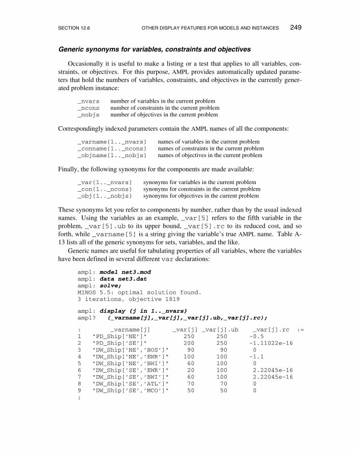
Generic synonyms for variables, constraints and objectives
Occasionally it is useful to make a listing or a test that applies to all variables, con-straints, or objectives. For this purpose, AMPL provides automatically updated parame-ters that hold the numbers of variables, constraints, and objectives in the currently gener-ated problem instance:
_nvars number of variables in the current problem_ncons number of constraints in the current problem_nobjs number of objectives in the current problem
Correspondingly indexed parameters contain the AMPL names of all the components:
_varname{1.._nvars} names of variables in the current problem_conname{1.._ncons} names of constraints in the current problem_objname{1.._nobjs} names of objectives in the current problem
Finally, the following synonyms for the components are made available:
_var{1.._nvars} synonyms for variables in the current problem_con{1.._ncons} synonyms for constraints in the current problem_obj{1.._nobjs} synonyms for objectives in the current problem
These synonyms let you refer to components by number, rather than by the usual indexednames. Using the variables as an example, _var[5] refers to the fifth variable in theproblem, _var[5].ub to its upper bound, _var[5].rc to its reduced cost, and soforth, while _varname[5] is a string giving the variable’s true AMPL name. Table A-13 lists all of the generic synonyms for sets, variables, and the like.
Generic names are useful for tabulating properties of all variables, where the variableshave been defined in several different var declarations:
ampl: model net3.modampl: data net3.datampl: solve;MINOS 5.5: optimal solution found.3 iterations, objective 1819
ampl: display {j in 1.._nvars}ampl? (_varname[j],_var[j],_var[j].ub,_var[j].rc);
: _varname[j] _var[j] _var[j].ub _var[j].rc :=1 "PD_Ship[’NE’]" 250 250 -0.52 "PD_Ship[’SE’]" 200 250 -1.11022e-163 "DW_Ship[’NE’,’BOS’]" 90 90 04 "DW_Ship[’NE’,’EWR’]" 100 100 -1.15 "DW_Ship[’NE’,’BWI’]" 60 100 06 "DW_Ship[’SE’,’EWR’]" 20 100 2.22045e-167 "DW_Ship[’SE’,’BWI’]" 60 100 2.22045e-168 "DW_Ship[’SE’,’ATL’]" 70 70 09 "DW_Ship[’SE’,’MCO’]" 50 50 0;
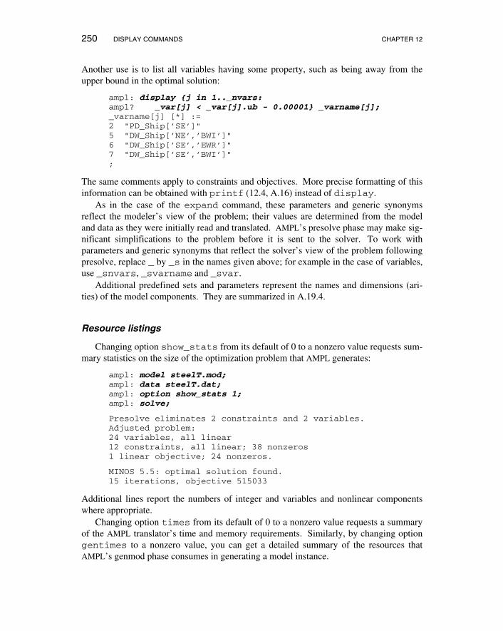
250 DISPLAY COMMANDS CHAPTER 12
Another use is to list all variables having some property, such as being away from theupper bound in the optimal solution:
ampl: display {j in 1.._nvars:ampl? _var[j] < _var[j].ub - 0.00001} _varname[j];_varname[j] [*] :=2 "PD_Ship[’SE’]"5 "DW_Ship[’NE’,’BWI’]"6 "DW_Ship[’SE’,’EWR’]"7 "DW_Ship[’SE’,’BWI’]";
The same comments apply to constraints and objectives. More precise formatting of thisinformation can be obtained with printf (12.4, A.16) instead of display.
As in the case of the expand command, these parameters and generic synonymsreflect the modeler’s view of the problem; their values are determined from the modeland data as they were initially read and translated. AMPL’s presolve phase may make sig-nificant simplifications to the problem before it is sent to the solver. To work withparameters and generic synonyms that reflect the solver’s view of the problem followingpresolve, replace _ by _s in the names given above; for example in the case of variables,use _snvars, _svarname and _svar.
Additional predefined sets and parameters represent the names and dimensions (ari-ties) of the model components. They are summarized in A.19.4.
Resource listings
Changing option show_stats from its default of 0 to a nonzero value requests sum-mary statistics on the size of the optimization problem that AMPL generates:
ampl: model steelT.mod;ampl: data steelT.dat;ampl: option show_stats 1;ampl: solve;
Presolve eliminates 2 constraints and 2 variables.Adjusted problem:24 variables, all linear12 constraints, all linear; 38 nonzeros1 linear objective; 24 nonzeros.
MINOS 5.5: optimal solution found.15 iterations, objective 515033
Additional lines report the numbers of integer and variables and nonlinear componentswhere appropriate.
Changing option times from its default of 0 to a nonzero value requests a summaryof the AMPL translator’s time and memory requirements. Similarly, by changing optiongentimes to a nonzero value, you can get a detailed summary of the resources thatAMPL’s genmod phase consumes in generating a model instance.

SECTION 12.7 GENERAL FACILITIES FOR MANIPULATING OUTPUT 251
When AMPL appears to hang or takes much more time than expected, the display pro-duced by gentimes can help associate the difficulty with a particular model compo-nent. Typically, some parameter, variable or constraint has been indexed over a set farlarger than intended or anticipated, with the result that excessive amounts of time andmemory are required.
The timings given by these commands apply only to the AMPL translator, not to thesolver. A variety of predefined parameters (Table A-14) let you work with both AMPLand solver times. For example, _solve_time always equals total CPU secondsrequired for the most recent solve command, and _ampl_time equals total CPU sec-onds for AMPL excluding time spent in solvers and other external programs.
Many solvers also have directives for requesting breakdowns of the solve time. Thespecifics vary considerably, however, so information on requesting and interpreting thesetimings is provided in the documentation of AMPL’s links to individual solvers, ratherthan in this book.
12.7 General facilities for manipulating output
We describe here how some or all of AMPL’s output can be directed to a file, and howthe volume of warning and error messages can be regulated.
Redirection of output
The examples in this book all show the outputs of commands as they would appear inan interactive session, with typed commands and printed responses alternating. You maydirect all such output to a file instead, however, by adding a > and the name of the file:
ampl: display ORIG, DEST, PROD >multi.out;ampl: display supply >multi.out;
The first command that specifies >multi.out creates a new file by that name (or over-writes any existing file of the same name). Subsequent commands add to the end of thefile, until the end of the session or a matching close command:
ampl: close multi.out;
To open a file and append output to whatever is already there (rather than overwriting),use >> instead of >. Once a file is open, subsequent uses of > and >> have the sameeffect.
Output logs
The log_file option instructs AMPL to save subsequent commands and responsesto a file. The option’s value is a string that is interpreted as a filename:
ampl: option log_file ’multi.tmp’;

252 DISPLAY COMMANDS CHAPTER 12
The log file collects all AMPL statements and the output that they produce, with a fewexceptions described below. Setting log_file to the empty string:
ampl: option log_file ’’;
turns off writing to the file; the empty string is the default value for this option.When AMPL reads from an input file by means of a model or data command (or an
include command as defined in Chapter 13), the statements from that file are not nor-mally copied to the log file. To request that AMPL echo the contents of input files,change option log_model (for input in model mode) or log_data (for input in datamode) from the default value of 0 to a nonzero value.
When you invoke a solver, AMPL logs at least a few lines summarizing the objectivevalue, solution status and work required. Through solver-specific directives, you can typ-ically request additional solver output such as logs of iterations or branch-and-boundnodes. Many solvers automatically send all of their output to AMPL’s log file, but thiscompatibility is not universal. If a solver’s output does not appear in your log file, youshould consult the supplementary documentation for that solver’s AMPL interface; possi-bly that solver accepts nonstandard directives for diverting its output to files.
Limits on messages
By specifying option eexit n, where n is some integer, you determine how AMPLhandles error messages. If n is not zero, any AMPL statement is terminated after it hasproduced abs(n) error messages; a negative value causes only the one statement to beterminated, while a positive value results in termination of the entire AMPL session. Theeffect of this option is most often seen in the use of model and data statements wheresomething has gone badly awry, like using the wrong file:
ampl: option eexit -3;ampl: model diet.mod;ampl: data diet.mod;diet.mod, line 4 (offset 32):
expected ; ( [ : or symbolcontext: param cost >>> { <<< FOOD} > 0;
diet.mod, line 5 (offset 56):expected ; ( [ : or symbol
context: param f_min >>> { <<< FOOD} >= 0;
diet.mod, line 6 (offset 81):expected ; ( [ : or symbol
context: param f_max >>> { <<< j in FOOD} >= f_min[j];
Bailing out after 3 warnings.
The default value for eexit is –10. Setting it to 0 causes all error messages to be dis-played.
The eexit setting also applies to infeasibility warnings produced by AMPL’s pre-solve phase after you type solve. The number of these warnings is simultaneously lim-
SECTION 12.7 GENERAL FACILITIES FOR MANIPULATING OUTPUT 253
ited by the value of option presolve_warnings, which is typically set to a smallervalue; the default is 5.
An AMPL data statement may specify values that correspond to illegal combinationsof indices, due to any number of mistakes such as incorrect index sets in the model,indices in the wrong order, misuse of (tr), and typing errors. Similar errors may becaused by let statements that change the membership of index sets. AMPL catches theseerrors after solve is typed. The number of invalid combinations displayed is limited tothe value of the option bad_subscripts, whose default value is 3.


![HP Color LaserJet 5/5M Printerh10032. type indicates text visible on the printer display or commands seen on the computer display. [Keyface] indicates one of several keys on the printer](https://img.dokumen.tips/doc/110x75/5b1b2c467f8b9a2d258e4650/hp-color-laserjet-55m-type-indicates-text-visible-on-the-printer-display-or-commands.jpg)


![Introduction to Linux commands and Vim - Department of ... · PDF fileIntroduction to Linux commands and Vim ... file1 [file2...] •Display the content of text files and to combine](https://img.dokumen.tips/doc/110x75/5aa6f6217f8b9ad31c8b56a7/introduction-to-linux-commands-and-vim-department-of-to-linux-commands-and.jpg)


