DISCUSSION OF THE DANISH DATA ON LARGE FIRE INSURANCE LOSSES

SIDNEY I. RESNICK

Conlell Umver~ttv

ABSTRACT

Alexander McNel l ' s (1996) study of the Damsh data on large fire insurance losses provides an excellent example of the use of extreme value theory m an m~portam apphcat |on context. We point out how several alternate statistical techmques and plot- ting devices can buttress McNel l ' s conclusions and provide flexible tools for olher studies

KEYWORDS

Heavy tails, regular vanat |on, Hill estimator, Polsson processes, linear programming, parameter esumatlon weak convergence, cons|stency, esumatlon, independence, auto- correlauons.

t I N T R O D U C T I O N

McNefl ' s (1996) interesting study of large fire insurance losses provides an excellent case history illustrating a variety of extreme value techniques The goal of my return'ks Is to show additional techmques and plotting strategies which can be employed for sm~flar data.

Our remarks concentrate on the following: • Dmgnostics for assessing the appropriateness of heavy tailed models • Diagnostics for testing for independence.

It is customary in many insurance studies |nvolvmg heavy tailed phenomena to as- sume independence without actually stausucally checking this important fact so some attention is given to this issue

2 APPROPRIATENESS OF HEAVY TAILED MODELS

Given a particular data set, there are various methods of checking that a heavy tailed model is appropriate. The methods given below (these are also reviewed in Resnlck 1995, 1996, Feigln and Restock, 1996) supplement the techniques discussed by McNeil such as mean excess plot,, and QQ-plots against exponenual quantdes. Unhke the mean excess plot, the following methods do not depend on existence of a finite mean for the marginal distribution of the stationary time series This is m~portant since it ~s becoming clear that it is not difficult to find examples of heavy tailed data which

AS'] IN BULLETIN, Vol 27, No I. 1997 pp I ~9-151

140 SIDNEY I RESNICK

require infinite mean models for adequate fits (See for example the teletraffic exam- pies m Restock (1995, 1996)).

For the discussion that follows, we suppose {X,,, n > I } is a stationary sequence and

that

PIXi > xl = x "~ H x ) . ~. ~ o o (2 1 )

where L ts slowly varying and ct > 0 Consider the following techniques (1) The Htl l plot. Let

Xi~ ) > Xc2 ~ > . > X~,,~

be the order statistics of the sample X~,. , X,, We pick k < n and def, ne the Hill estn- mator (Hdl, 1975) to be

1 ~ log X~'-----L-) Hk'n = k ~=1 X(/~+l)

Note k ~s the number of upper order statistics used m the estmaatlon The Hill plot ~s

the plot of

( (L Hi.I,,), I < Ic < n)

and ff the {X,,} process ns lid or a linear moving average or satnsfies certain mtxmg

condtt,ons then since HA.,, P > a -I as n --~ oo k/n --, 0 the Hall plot should have a

stable regime sitting at height roughly ~x See Mason (1982), Hsmg (1991), Restock

and Stanca (1995, 1996a), Rootzen et al (1990), Rootzen (1996). In the Hd case, under a second order regular variation condition, H~, is asymptotically normal wnth asymp- totnc variance I / ~ (See de Haan and Restock, 1996)

(2) The .~mooHtll P lo t The Hill Plot often exh~bnts extreme volatnhty whuch makes finding a stable regm~e m the plot more guesswork than scnence and to counteract this,

Restock andSt.~nc~ (1996a) developed a smoothing techmque y,eldmg the smooHlll plot Puck an integer u (usually 2 or 3) and define

smooH~,,, (. 1)----~" y~ Hi.,, J=/~+l

In the hid case when a second order regular variation cond~tnon holds, lhe asymptotic

varmnce of~mooH~, , is less than that of the Hill estimator, namely.

I 2 log u c~ 2 u (I - u )

The senstttvtty of the Htll esttmate to the chotce of k corresponds m McNefl's work to the sensitivity of the fit of the generalized Pareto to the data to the choice of threshold

Perhaps some comparable smoothing technique would help m GPD fitting.

(3) Al t p lot t ing, C h a n g i n g the ~cale. As an alternatnve to the Hill plot, it ts sometu- mes useful to dxsplay the mfrormatton provided by the Hall or smooHlll estnmatlon as

DISCUSSION OFTHE DANISH DATA ON LARGE FIRE INSURANCE LOSSES 141

and smallarly for the smooHtll plot where we write Fy-[ for the smallest integer greater or equal to y > 0 We call such plots the alternanue Hill plotabbrcviated AItHlll and

the alternative smoothed Hill plot abbrevmted AltsmooHfll The alternative display is sometimes revealing since the mmal order statistics get shown more clearly and cover a bigger portion of the displayed space. However, when the data is Pareto or nearly Pareto, this alternate plotting device is less useful since in the Pareto case, the Hill estimator applied to the full data set is the maxmmm likelihood estimator and hence the correct answer is usually found at the right end of the Hill plot

(4) Dynamic and static QQ-plots As we did [-'or the Hill plots, pick k upper order statistics

X(i ) > X(2 ) > . > X(k )

and neglect the rest Plot

{ ( - l o g 0 - k---~), log X¢j)), I < j' < k}. (2.2)

If the data are approximately Pareto or even if the marginal tall is only regularly va- rying, this should be approxmlately a straight hne with slope I/~. The slope of the least squares line through the points Is an esumator called the QQ-estunator (Kratz and Restock. 1996) Computing the slope we find that the QQ-estlmator is given by

1 ,

i Y-,i--, ,, or---k,,, (2 3)

k Z~=I ( - log( k+-I ))- - ( k I

There are two different plots one can make based on the QQ-est lmator There is the A

dynamic QQ-plot obtained from plomng {k, l /a- l t , , , , l < k _< n} which is similar to the

Hill plot. Another plot, the statfc QQ-plot, is obtained by choosing and fixing k, plot- ting the points m (3 2) and putting the least squares line through the points while com- puting the slope as the estimate of ~-~

The QQ-estlmator is consistent for the nd model if k --~ ~ and k/n ---) 0 and tinder a second order regular vm lanon condmon and further restriction o n k(n), it is asymptoti- cally normal with asymptotic variance 2 / ~ Th~s is larger than the asymptotic variance of the Hill estimator but the volatility of the QQ-plot always seems to be less than that of the Hill estmlator.

(5) De Haan's moment es,mator McNeil discusses the extreme value distributions (see also Restock, 1987; de Haan, 1970, Leadbette~ et al, 1983, Casnllo, 1988, Em- brechts et al 1997) which can be parameterlzed as a one parameter family

G¢ ( a ) = exp{-( l + ~x)-~--' }, ~ ~ 91,1 +~.r > 0

When ~ = 0, we interpret Go as the Gumbel distribution

Go(x) = e x p { - e - ' }. x ~ 9l.

142 SIDNEY I RESNICK

A distribution whose sample maxima when properly centered and scaled converges in distribution to G~ is said to be in thedomam of attraction of G¢ which m McNetl ' s notation is written F6 MDA(G~) If ~ > 0 and F~ MDA(G 0 then I - F ~ RV_i/~ De

Haan 's moment est imator ~,,, (Dekker 's , Elnmahl, de Haan, 1989, de Haan. 1991,

Dekkers and de Haan, 1991; Resntck and Startca, 1996b) ts designed to estimate ~ =

1/C~ Note that ~x.,,, like the Hill estimator, is based on the k-largest order statistics

Since most common densities such as the exponentml, normal, gamma and Welbull densities and many others are m the MDA(Go), the domain of attraction of the Gumbel distribution, this provides another method of dectdmg when a distribution ts heavy

tailed or not If ~.,, is negative or very close to zero, there is considerable doubt that

heavy taded analysis ~hould be apphed and the moment esttmator is usually much

more rehable in these circumstances than the Hill estmlator In particular, when ~ = 0, the Hill estimator is not usually informatwe and the moment estm~ator does a much better job of identffymg exponential ly bounded tails Smoothed versions of the mo- ment est imator can also be devised (Resntck and Starlca, 1996b) which overcome

volatility in the plot of {k,~x ,,, I _< k _< n}

o

D a n i s h D ~ . t e t Q Q D a n i s h

~ 0 0 ~ 0 0 0 ~ 5 0 0 2 0 0 0

FIGURL2 I T~plot and QQ plot of Damsh data

Q Q D a n i s h . a l l

° . ~ . ~ . . . . . . . . % . . . . . ~ , . ,

P ~ r f l t D a n i s h

°i FIGURE 2 2 QQ plot of Ddm~h oil dala and parameter cst]mate

DISCUSSION OF THE DANISH DATA ON LARGE FIRE INSURANCE LOSSES 143

-R

o

Hi l l a n d D y n a m i c Q Q

0 5 0 0 1 0 0 0 1 5 0 0 2 0 0 0 0 5 0 0 1 0 0 0 1 5 0 0 2 0 0 0 n u m b e r of o r d e r 5 t e t l s t l c s n u m b e r o f o r d e r 8 te t l s t Jcs

FIGURE2 3 Hdl and QQ-ploI of Damsh data

Figure 2 1 gives a time series plot of the 2156 Danish data consisting of losses over one million Danish Krone (DKK) and the right hand plot is the QQ-plot (2 2) of this data yielding a remarkebly strmght plot Figure 2.2 gives the QQ-plot of all of the 2492 losses recorded In the data set labeled danish.all and shows why McNeil was statistically wise to drop losses below one mdhon DKK (In the left hand plot the data is scaled to have a range of (0.3134041, 263 2503660) and the dots below hexght 0

represent the 325 values which are less than 1 m the scaled data.) The right hand plot in Figure 2 2 puts a line through the QQ-plot of the losses above one milhon and yields an estimate of a = I 386 Using only the largest 1500 order statistics and then estimating t~ from the slope of the LS line produces an estimate of a = 1 4

We next attempted to estimate a by means of the Hill plot Figure 2 3 shows a Hill plot side by side with the dynamic QQ-plot . Because the plot m the right side of Figure 2 I is so straight, we tend to trust the Hill plot near the right end of the plot This is because the ~tralght plot m Figure 2 I mdlcate~ the underlying distribution ~s close to Pareto and for the Pareto dlstnbuuon the maxmmm likelihood esumator of the shape parameter ~s the Hill esumator calculated using all thc data This analysis Is confirmed by the excellent fit achieved by McNeil using a GPD with ~ = 0 684 or

= 1.46 corresponding to losses exceeding a threshold of 20 million DKK. Such a GPD is a shlftcd Pareto

On the other hand, examining the altHlll and al tsmooHdl plots in Figure 2 4 makes it seem unlikely that ~ could be as large as 2 01 which is what Is given m M c N e d ' s Figure 7. This corresponds to a ~ = 0 497. Our methods indicate a likely value of c~ = 1 45

In Figure 2 5 we present four views of the moment esumator ~k.,, ol ~ = f la . The

upper right graph and the lower two graphs are m a l t scale where k, I _< k_< n is replaced by Vn°]. 0 <_ 0 _< I Interestingly, we see here and m the four views of the Hall plot, that when the data are very close to Pareto, the alt scale is not advantageous

] 44 SIDNEYI RESNICK

When the data ~s close to Pareto, the rehable part of the graph ~s toward the end and this is the part of the graph under emphasized by the air scale The s~tuatmn ~s very different for something hke stable data (Restock, 1995) where the tradmonal Hill plot

is incapable of identifying the correct value of ~ but the alt plot does a superior job. Based on an amalgam of the QQ, Hill and moment plots, we settle on an esumate of

a = l . 4 o r ~ = 71

o.

~ . 04

ID

E

Hill pl0t AltHill o.

Q. OD

500 1000 1500 2000 0.2 0 4 0 6 0.8 1 0 number of order statistics theta

AltsmooHill AItHill and AItsmooHil l q

Ea.o~

0 2 0.4 0 6 0 8 0.2 0 4 0 6 0 8 1.0 theta theta

FIGURE2 4 Hill and smooHfll plot s., tor Dam~h data

3 TESTING FOR INDEPENDENCE

We outline several tests for mdependence which can help reassure the analyst that an ud model is adequate and that ~t ,s not necessary to try to fit a stationary ame series

with dependencies to the data. Some of our tests are motivated by our experience trying to fit autoregressive processes to heavy taded data

Here .s a survey of several methods which can be used to test independence Some of these are based on asymptotic inethods using heavy tailed ,malysls and the rest are standard rune series tests of homogeneity

(1) Method based on sample acf: An exploratory, informal method for testing for independence can be based on the sample autocorrelatlon funcnon ,6(h) where for h

any posmve integer / t -h

,b(h) = 2. , ,=, (X, - X ) ( X , . h -- X )

Z 2 , -

DISCUSSION OF THE DANISU DATA ON LARGE FIRE INSURANCE LOSSES 145

In many studies of heavy tailed data, the centering by the sample mean is omitted since If mathematical expectation does not exist, there is no advantage or sense to

centering by the sample mean However, since our chosen value of ~ =1 4 imphes EIXJ < oo, we have decided to include the centering From Davis and Resnlck (1985a), if {X,} are nd with regularly varying tall probabilities, then

hnl /~(h)={ I' I f h=0 , , , ~ 0, lfh :*: 0.

Thus, ~f upon graphing /3(h), h = 0, ., n - h we get only small values for h # 0 there is no evidence against independence The Matt distribution of /~(h), h = I, . , q is known (Daws and Resntck, 1985b, 1986 Corollary 1) but it is somewhat difficult to work with and the percentiles must be calculated by simulation It is important to leahze that the 95% confidence bands drawn by a typical statistics package like Splus are drawn using Bartlett 's formula (Biockwell and Davis, 1991) on the assumption

that the data is Gausslan or at least has flmte fourth moment This assumption is to- tally inappropriate for heavy tailed data and the confidence band must be drawn taking ,nto account the heavy tailed limit distribution for f3(h), h = I , . , l

O

¢¢1

g

g 8 E ~

O

O

~d ~ g

o E ¢5

moment estimator

? O

AI t p l o t

o ~ E . ¢

0 500 1000 1500 2000 o 0 4 0.6 0.8 1.0 number of order statistics theta

A l t s m o o AI t a n d a l t s m o o p lo t O

o g E , ¢

0 3 0 4 0.5 0 6 0 7 0 8 o 0 4 0.6 0 8 1 0 theta theta

FIGURE2 5 Moment esmnalor plots for Damsh data

We discuss Jmplementauon of the acf based procedure when 1 < o~ < 2 since m the case of the Danish loss data we have settled on an estnnate of o~ = 1.4 Suppose { Yi,

, Y.} are lid non-negative random variables satisfying

P[,~ > x J - x - a L ( x ) , x ~ o o , l < ~ < 2

146 SIDNEY I RE£NICK

where L is slowly varying From Corollary 1, page 553 of Davis and Restock (1986), if we set /3y (]1) to be the lag h sample acf for Y~, . . Yo, then we have

hm P[Ig,~-' b,~ tSr(h ) _< x l = PIUh / V o -< x] / t . - . ) ~

where Uh is a one sided stable random variable with index o~ = 1 4 and V o is a posture

stable random variable with index cd2 = 0.7 and b,, is the solution to

PI Yz > x I = I / n

and /~,, is the soluhon to

P[YJY2 > x ] = IIn

Thus an approximate symmetric 95% confidence window for the sample correlauons

of the Y's would be placed at _+l/~,,/b,~ where /sausfies

P[luh/v01-< l] = .95.

We estimate the 95%-quantlle of IUj/Uol by sm]ulatlon and if we assume the dlstnbu- uon of Y,'s ~s Pareto from some point on, we find

i b,, l( n I -'`a b,;

The assumpuon o f a Pareto dlstnbuuon seems mild m view of Figure 2 2 and the good fit found by McNed of the GPD with posluve shape parameter

F=gure 3 I presents this techmque apphed to the Damsh loss data. No sDke is protruding trom the band and hence this acf based techmque does not provide any evidence against the assumpuon of independence.

9 5 % C o n f i d e n c e B a n d

Q

9

I I , ] i ' i ' )

5 1 0 1 5 2 0 L a g

FIGURE 3 1 95% confidence band for the acf of the Dam~h loss data

DISCUSSION OF ]'HE DANISH DATA ON LARGE FIRE INSURANCE LOSSES 147

(2) Test~ based on asymptotic theory Estm~ators of autoregresswe coefficients for heavy tailed time series can be used to fashion tests for independence against autore- gresswe alternatives If the autoregress~on ~s described as

P

X, ='~-'~,X,_, +Z, , t = 0 , 1 ....

where {Z,} are lid heavy tailed residuals, then we test if

4'1 = - = Or, = O,

that ~s independence, by rejecting when the maximal estimated coeff|cient

P

is too large This procedure has been mlplemented by Felgm. Restock and Statics1 (1996) based on hnear programming (LP) estimators under the assumption that the lid heavy taded residuals {Z,} are non-negauve. See also Felgln and Restock (1993)

It would not be possible to fix the size of the LP test if the hmlt distribution of the LP estimator d~d not considerably sunphfy Fortunately it does under the null hypothe- sis of independence and we then have

b,,(6,(,~), . , 6 , 0 ~ ) ) ~ L --- (V i - ' . . . . V~7 ~ )

where for .~, > 0, ~ = 1, , p we have that

P[V, < x , . l = 1. ,p]=expl- j~f F(dy I) F(dye)} (3 2) - ~. ~'.)~10 ~1" = " ) ' I X I "

This means that i f we want a 0 05 level rejection region, we should reject when

v p I~ , (n) l > K (05 ) where K(05) is defined by t=]

and to find an approxmlate value of K(.05) we write

P ~,(n)l> g ( 05) = P L,>b,,K(05) <_pP[L,>b,,K(O5)]=pe -c(°~KC°5:, (33)

where c = E(Z{ ~) Thl~ yields

K( O5)= I-I°g('-O5 / p) ) _ ( l °g (~Op) / I / a

b. b,,

We need to esumate c~, c and b. One way to do this is to use the QQ-plot (Fe~gm. Restock andStfincfi, 1996; Kratz and Restock. 1996) which yields both /~. (as the

148 SIDNEY I RESNICK

intercept of the fitted line) and ~ (as the reciprocal of the slope of the fitted line) and then we can get

= ,,-' x 7 t= l

The asymptotic test is implemented and shown In Figure 3 2 None of the estimated coefficient values extend above the bar representing K(05) so this method provides no evidence against the hypothesis of independence

A s y m p t o t i c T e s t

Q

Q

g I I I I 2 4 6 8

n u m b e r o t c o e f f i c i e n t s

FIGURE3 2 Asymptotic test for independence for the Damsh loss data

1 0

(3) Standard tests of randomness. There are several standard time series tests of

randomness (Brockwell and Davis, 1991, Section 9 4) which are non-parametric and can be employed In the present context. We give some examples below We use the notation

Z,, ~ AN(p,,, a,~ )

as shorthand to mean that (Z,, - p , , ) l o , ~ N(O, I)

( I ) Turn ing point test [ f T is the number of turning points alnong X~,. , X,, then under the null hypothesis that the random variables are l id we have

T ~ AN(2(n - 2) 13, (I 6n - 29) 190)

and thls can be used as the basis of a test

(2) Difference-sign test Let S be the number of t = 2, , n such that X, - X, ~ is po- sitive Under the null hypothesis that the random varlablesX~ . . . . X,, are lid we have

S - A N ( ~ ( n - l),(n + 1)/12).

DISCUSSION OF THE DANISH DATA ON LARGE FIRE INSURANCE LOSSES 149

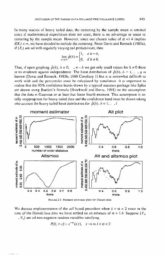
(3) Rank test Let P be the number of pairs (~,j) such that Xj > X, lo r j > t and t = I,

, n - I Under the null hypothesis that the random variables X~, , X,, are lid we have

- A N ( ~ n ( n - I ) , n (n - l ) ( 2 n P + 5)/8).

We would reJect the lid hypothesis at the 0 05 level If any of these standardized vana- bles had an absolute value greather than 1 96. All of these tests are implemented m the

Brockwell and Davis (1991) package ITSM. Data can easily be imported into their

program and tested within the package for randomness. We canied out these tests on the Danish loss data using ITSM and achieved the

following results Turning points 1409 AN (1436 00, 19 572) Diffelence-slgn 1079 AN (1077.50, 13.412)

Rank test 1055894 AN (1161545, 50071 902)

The rank test reJects the hypothesis of independence at the 5% level The turning points and difference-sign tests fail to reJect.

(4) Stability testmg on subsets of the data An informal but useful technique us to

take a stam~tnc, such as the sample acf, and compute it relative to different subsets of the sample If the data is uud, the values of the statistic should be smaular across diffe- rent subsets. For the sample acf, nf the graphs of /gu (h), h = I . . . . . q look different for different subsets, then one should be skeptical of the correctness ot the rid assumption Often ut is enough to split the sample unto halves or thirds to generate some skepticism One

could make acf subset plots for the Damsh data but since the acf values are not signifi-

cantly different from 0, there seems httle point to pursuing this diagnostic in this case

(5) Permutatton te~t for independence. Another approach to testing for indepen- dence in tmle series analysis us based on permutation tests. Here we can use any desi- red statistic that is designed to measure some form of dependence between successive

data Thus statistic umght be a maxm~um autocorrelatuon or partial autocorrelatlon, or it may be a maximal autoregressuve coefficient estimated by the linear programming

paradigm The permutation test us based on companng the observed value of the statistic with

the permutation distribution of that statistic - - that us with the distribution of values of the statistic under all the possible permutations of the time series data If there us no

dependence structure m the data, then the observed value should be a typical value for this reference permutation distribution. If there us some dependence of the type to which the statistic us sensitive, then the observed value should be extreme with respect to thus reference distribution

This approach allows one to perform tests without relying on the asymptotic theory for the partlculai statistic. As we have seen earlier, the asymptotic distribution for

1 5 0 SIDNEY I RIz.SNICK

P v ,~,(n) I=l

revolves vattous parameters that have to be esumated Moreover, the fact that we are not sure of the rate of convergence to the asymptotic distribution, also suggests the

precautionary tactic of using a pernautat~on test In the implementation we use below, we approxmaate the p - va lue of the actually

observed statistic This is achieved by generating 99 permutations of the time series, computing the statistic for each one, and counting the number (C) of these that are greater than or equal to the actually observed statistic The p-value is approximated by (1+C)%. The statistics considered are the maximum absolute autocorrelauon (macf),

the maximum absolute partial autocorrelat~on (mpacf), and the maximum absolute linear programming coefficient estimate (mphl) In each case, one must specify the value of p, the order over which the maxunum is taken

For the Damsh loss data, we took the order to be 10 and ran the tests yielding the tollowmg p-values

maximum autocorrelatlon 0.52

maximum partial autocorrelatlon 0.51 maximum LP coefficient 0 22

and thus at a reasonable level, none of these tests would reject independence

4 CONCLUDING REMARKS

There is very little evidence argtung against the hypothesis of independence and it seems McNell 's presumption that the data were independent was a safe assumption to make for this data set Independence is not that common among teletraffic of finance data in my experience and thus should be treasured in the present insurance context Fittmg dependent data with a heavy tailed stationary time series model can be a frus- trating business (see Restock, 1996b, Felgln and Resnlck, 1996) so when one conclu-

des the data can be modelled as ud, a loud sigh of rehef is heard The sensitivity of the estmmtion and fitting methods to the choice of threshold or

the choice of the number of order statistics used in estimation ~s a persistent and troubhng theme In McNefl 's and my remarks. This seems inherent m the heavy tall and extreme value methods It ~s not clear at this point how much the techmques can be improved to reduce sensmv~ty to choice of k or threshold Smoothing techniques

and alternate plotting help but are not a universal panacea. It is encouraging to see the accumulating mass of theoretical and software tools

which can be used to analyze such data sets

REFERENCES

BROCKWELI, P and DAVIS, R, Tmw Setmv Theo O' and MeHlud.~, 2 na edmon, Sprmger-Verlag, New York 1991

BRt~CKWEI L, P and DAVlq, R ITSM Apt Inteta~ttve Tram Se;ws Modelhnt~ PacLageJor the PC, Sprmgcr- Verlag, New York 1991

CASTII.[ O, ENRIQUE, Ettteme Value Theor~ tit Engineering, Academic Pre,,s. San Diego, Cahforma, 1988

DISCUSSION OF THE DANISH DATA ON LARGE FIRE INSURANCE LOSSE.S ] 5 1

DAVIS. R and RESNICK, S , Lnn~t theory for moving ave]ages at random varmbles with regularly varying Iml probabilities, Ann Probability 13 (1985a). 179-195

DAVIS, R and RESNICK, S , More lantt theory for the ~aalple correlation function of moving averages. Stoch,lstJc Proces,,cs and their Apphcallons. 20 (1985b). 257-279

DAvis, R and RESNIC~ S , Lmlll theory for the sample covanance and correlatmn functions of moving averages, Ann Statist 14 (1989), 533-558

DEKKERS. A , EINMAHL, J , and HAAN, L DL. A inolltent e~ttlnator /'or the tndea of an eatreme value dl3tttbu- tlon, Ann Statist 17 (1989), 1833-1855

DEKKERS, A and HAAN, L DE, On the estimation of the extreme value Index and large quantde estimation, Ann Statrst 17 (1989), 1795-1832

EMBRECHTS, P. KLUPPELBERG, C and M IKOSCH. T. Modelhng E.~trema/Event~ for Iil~aram e and Ftnallce. To appear, Spnnger-Verlag, Hezdclberg. 1997

FIzlGIN. P and RESNICK. S . Limit dr~tttbatton~ fat haeal proglammmg tmle aelte~ e~ttmator~. Stochastic Piocesses and then Apphcat]ons 51 (1994). 135-166

FEIGIN. P and RESNICK, S , Pttfall~ of fitting autoregre~lve models fi)l heavy-taded time aeries. Avadable ,it hllp/www orlc cornell edu/trhst/trhst htlml as TR 1163 pc Z (1996)

FEIGIN, P , RESNICK S , and St~ne~, C, Te¢ttng Jar independence tn heav~, tailed and positive rnnol,atton ttale ~elte~. Stochastic Model~ 11 (1995), 587-612

HAAN, L DE, On Regulal Valtatton alrd It~ Apph~atton to the Weak Convergence of Sample Eatretne,~. Mathematlc,ll Cenue Tract 32, Mathematical Centre, Amsterdam, Holland, 1970

HAAN. L DE. E.~trelne Value Stattstrca, Lecture Notcs. Econometric Inshlute, Erasmus University. Rotter- dam ( 1991 )

HAAN, L DE and RESNICK, S, On as~otptottc tlortttaltt 3' of the Ihll esttolatot, TR1155 ps Z avadable at http/www or le comell edu/tt hst/trhst htlml (1996)

HILL, B , A smlple approach to reference about the tad of a dtstnbtmon, Ann Statxst 3 (1975), II 63-II 74 HSING, T, Extreme value theory for suprema of random varmbles with regularly varying tail probabdmes,

Stoch Proc andthe]rAppl 22 (1986). 51-57 KRATZ, M and RESNICK. S . Tire qq-e~tanator and heavv tads. Stochastic Models 12 (1996). 699-724 LEADBETTER, M , LINDGREN, G and ROOTZEN, H , t:',~treme~ and Related Propertte~ of Random Sequence~

and Procea~e~. Spnng Vcrlag, New York, 1983 MASON, D, Laws of large numbers for sums of extreme valucs, Ann Probablhly 10 (1982), 754-764 MCNEIL, A , Estm~atmg the fads of loss seventy d~,,tnbut~ons using extreme value theory, P~eprmt Dept

Mathematics. ETH Zentrum, CH-8092 Zurich (1966) RE,SNICK, S , Ertleme Valuer. Reg,lat Vattatton, and Point Pto~esse~, Sprlnger-Vellag. New Yolk. 1987 RESNICK, S . Hear~ tail modelhng and teletlaff tc data. Available as TR1134 ps Z at

http/www one eornell edu/trhst/trhst htlml, Ann Stal],,t (1995), (to appear) RE,SNICK, S . Wily noll-hneattttes ~all r~ttlr the heat y tailed modelel '~ da~,, Avmlable as TR1157 p~ Z at

http/www one cornell edu/trhst/trhst htlml, A PRACTICAL GUIDE TO HEAVY TAILS Stal~sl]cal Teehmques for Analysing Heavy Taded D~st~]bul]ons (Robert Adler, R,nsa Feldman, Murad S Taqqu, ed ). B~rkhauset, Boston I996, (to appear)

RESNICK, S ,rod Stfirtefi, C. ConstMenc 3 of Ittll'~ e,~ttn)atorfrn del)endetrt data. J Apphed P)obabdtty 32 (1995), 139-167

RESN~CR, S and St.]ncfi, C. Smoothrng the Hill e~ttmtttot. To appear J Apphcd Probab)hty (1996a) REqNICK, S and Stalled. C , Sn too th t t t~ the Ill01netlt e3trtttalo! of the eatteme i,ahre para t l l e l e t , Avalldhlt2 aq

TR1158 ps Z ,it http/www one eomell cdu/trhst/trhsl htlml, Preprmt (1996b) ROOTZEN, H, LEADBETI'ER. M and DE HAAN, L. Tail and quantde e~trmatton ]or ~ttonglv mramg ~tatton(try

sequencea. Technical Report 292, Cenlcr for Stochastic Processes. Department ol Statistics, Umvers~ty of North Carohna, Chapel Hdl. NC 27599-3260 (1990)

RoolTJ~ H The tail elnprtrt~al plo(e.~.sfi)l ~tattoaat~, ~equen(e~. Preprm! 1995 9 ISSN 1100-2255. Stu- dies m Statistical Quahly Control and Rehabhty. Chalmcrs Umvcrsrty ol Technology (1995)

SIDNEY I RESNICK

C o r n e l l Umver~' t ty ,

S c h o o l o f O p e r a t i o n s Re . search a n d Indua t r t a l E n g i n e e r i n g

Rhode,~ H a l l 2 2 3

I thaca . N Y 1 4 8 5 3 USA

E-mat / " s t d @ o r t e c o r n e l [ . e d u