Embed Size (px)
Citation preview

Discrimination in a universal health system: Explainingsocioeconomic waiting time gaps
Meliyanni Johara, Glenn Jonesa, Michael Keaneb, Elizabeth Savage∗a andOlena Stavrunovaa
aEconomics Discipline Group, University of Technology, SydneybDepartment of Economics, University of Oxford
FundingThis work was supported by the Australian Research Council [DP0986785].
AcknowledgementsWe thank Philip Haywood for clinical advice on mapping ICD codes in the hospital data to con-ditions relevant to hospitalisation. We also thank Pravin Trivedi, Jurgen Meineke, Lisa Cameron,Pedro Barros, Peter Sivey and participants at the 2nd Australasian Workshop on Health Economicsand Econometrics, for useful comments. The NSW Inpatient and Waiting Time data is providedby the NSW Department of Health. The use of the data has program ethics approval from theUniversity of Technology, Sydney.
∗Corresponding author: Elizabeth Savage, University of Technology Sydney, Economics DisciplineGroups, PO Box 123, Broadway NSW 2007 Australia. Email: [email protected] T:+61295143202. F: +61295147722.

Abstract
One of the core goals of a universal health care system is to eliminate discrimi-
nation on the basis of socioeconomic status. We test for discrimination using patient
waiting times for non-emergency treatment in public hospitals. Waiting time should
reflect patients’ clinical need with priority given to more urgent cases. Using data from
Australia, we find evidence of prioritisation of the most socioeconomically advantaged
patients at all quantiles of the waiting time distribution. These patients also benefit
from variation in supply endowments. These results challenge the universal health
system’s core principle of equitable treatment.
Keywords: Public hospital, waiting time, discrimination, decomposition analysis
JEL codes: I11, J7, H51, C14, C21
1

1 Introduction
Equity is one of the primary objectives of the universal health care systems of most European
countries, Canada, New Zealand and Australia. For example, one of the three guiding
principles of the UK National Health System since its foundation has been that access to
health care be based on clinical need, not ability to pay (Greengross et al., 1999). Similarly,
the Australian Medicare system has always been grounded on ‘access on the basis of health
needs, not ability to pay’ (Commonwealth of Australia, 2009). In contrast, in market-
based health care systems such as that of the United States, equity goals are not explicitly
formulated, and as a result, equity of access in the delivery of health services is under public
scrutiny. Low-income Americans, who are likely to be uninsured, not only use fewer health
services, but also receive less care when treated. Lopez et al. (2010) find that low income
patients presenting with chest pain in the emergency department are less likely to be treated
immediately and receive more basic cardiac testing than richer patients. Huynh et al. (2006)
report that compared to richer patients, low income patients have lower access to medical
care when sick (as measured by higher proportions of low income patients waiting six days or
more for a doctor appointment) and are more likely to go without care because of cost. They
also document a higher proportion of incorrect lab results or delay in receiving these results
among uninsured individuals compared to insured individuals. Similarly, Doyle (2005) finds
that hospitals provide less care (as measured by shorter length of stay and lower hospital
costs) to uninsured patients injured in automobile accidents compared to insured patients,
and that uninsured patients also have higher in-hospital mortality.
In universal health care systems, there has been less focus on the relationship between
access to health care and socioeconomic status, perhaps because their core equity principle
is simply assumed to hold. In this paper, we empirically test this presumption using waiting
times for elective, or non-emergency, procedures as the measure of access. In public hos-
pitals which are either free or heavily subsidised, waiting times are used to ration elective
procedures. Prioritisation rules require that patients with the most life-threatening or urgent
conditions, should be admitted first, regardless of their socioeconomic status. Countries dif-
fer in the way they implement clinical-based prioritisation rules. Canada and New Zealand
have developed explicit, systematic prioritisation rules in the form of scoring tools which in-
clude both clinical criteria and non-clinical social factors perceived to contribute to urgency,
such as inability to live and work independently. In contrast, in the UK, Spain, Sweden
and Australia, prioritisation is guided solely by clinical need but without an explicit scoring
procedure (see Siciliani and Hurst, 2005). Regardless of the method of implementation, there
2

is a common theme in universal systems that no patient should be discriminated against on
the basis of his/her socioeconomic status. In this paper, we test for discrimination in waiting
times for elective procedures using data from public hospitals in Australia.
To access hospital care for an elective procedure in Australian public hospitals, a patient
must obtain a referral from a GP for a specialist consultation. While the patient has free
choice of specialist, typically the GP’s advice will be relied upon to select the specialist. It
is the specialist who books the patient onto a hospital waiting list and assigns an urgency
category which determines priority on the waiting list. There are three urgency categories:
(i) ‘30 day’ is assigned to patients with ‘a condition that has the potential to deteriorate
quickly to the point that it may become an emergency’; (ii) ‘90 day’ is used for ‘a condition
causing some pain, dysfunction or disability, but which is not likely to deteriorate quickly
or become an emergency’; and (iii) ‘365 day’ is used for ‘a condition causing minimal or no
pain, dysfunction or disability, which is unlikely to deteriorate quickly and which does not
have the potential to become an emergency’. These urgency categories may be regarded as
the maximum waiting time beyond which treatment can be considered overdue and possibly
to carry health risks to patients.1
All Australian residents are eligible for public patient treatment at public hospitals by
hospital specialists but they may elect to be treated as a private (paying) patient in which
case they can choose their own specialist. Public patients are treated without charge and
are financed from block grants under health agreements between the Commonwealth and
State governments. Private patients are largely funded by insurance and this provides extra
revenue to the public hospital as well as fees to the treating specialist.2 Under hospital
financing agreements, both public and private patients in public hospitals should be subject
to exactly the same rationing rules.3 However, Johar and Savage (2010) find dramatic
waiting time differences between private and public patients waiting for the same procedure.
They also find, even within the same urgency category, much shorter waiting times for
1The number of patients waiting beyond the clinically recommended time is part of hospital qualitypublic reporting process however during the period of our data (2004-05) no financial sanction existed forperformance.
2Specialist fees and pharmaceutical costs for private patients are subsidised under the Australian Medicaresystem.
3The principles governing funding of public hospitals are defined in the Australian Health Care Agree-ments between the Commonwealth and each state. Principle 7 requires that all public hospital services toprivate patients should be provided on the same basis as for public patients. Access to public hospital careshould be on the basis of clinical need, not payment status. The Australian Health Care Agreement for 2003-08 can be found at http://www.health.gov.au/internet/main/publishing.nsf/content/B02C99D554742175CA256F18004FC7A6/$File/New%20South%20%20Wales.pdf
3

private patients in comparison to clinically comparable public patients. Because of the clear
financial incentives for hospitals and specialists to expedite private patient admissions in
public hospitals, we focus our analysis on public patients, who comprise 87% of all admissions
to public hospitals. Private patients incur hospital and medical charges in exchange for choice
of doctor and possibly a better standard of hospital accommodation which add to hospitals’
fixed budgets. Excluding them avoids potential confounding effects due, for example, to
preferences for different characteristics available with private care.
In principle a public hospital patient cannot choose the specialist who will perform the
procedure. However, if the referring specialist has the right to admit private patients at the
hospital to which the patient is referred, it is possible that the specialist may have influence
on scheduling and may even perform the procedure on the public patient. There is no direct
financial incentive for providers, both hospitals and specialists, to discriminate in favour of
high income public patients, however providers may benefit from prioritising high income
public patients by indirect means.
Discussions with hospital clinicians and administrators suggest that discrimination in
favour of richer patients may extend even beyond the hospital, to the referring trail from GP
to specialist and from specialist to hospital. In Australia, there is only anecdotal evidence on
this, however, GP’s influence in the referral trail has been found by Derrett (2005) using data
from New Zealand. She finds that GPs help their patients obtain faster hospital admission
by exaggerating their conditions when making specialist referrals.
Private health insurance provides an important link between patient income and ob-
served referral patterns. Since high income patients are more likely to have private health
insurance, they are more likely to use their insurance and elect to be admitted as private
patients. Because of the financial incentives to increase throughput from private patients for
both specialists and hospitals, preference may be given to patients from GP practices with
many privately insured clients (i.e., GP practices in high income areas). To strengthen this
relationship, this favourable treatment may extend to all patients from these GPs, including
those electing for public treatment. Similarly, hospitals have an incentive to give preference
to the referring recommendations of specialists who refer a greater volume of private patients
to the hospital.
These indirect incentives are facilitated by the considerable variability in waiting list
management procedures across hospitals. In principle, waiting time registers are managed by
the hospital administrator who has the discretion to schedule patients on the lists. However,
in some cases, the treating specialist, who may be contracted to the hospital, manages his/her
4
own waiting list, and in other cases, groups of specialists may jointly manage scheduling. In
addition, the absence of an explicit prioritisation scoring tool gives discretion to specialists in
assigning urgency class to patients, especially where there is low mortality risk from delayed
treatment.4 In either case, there is major involvement by specialists and it is difficult to
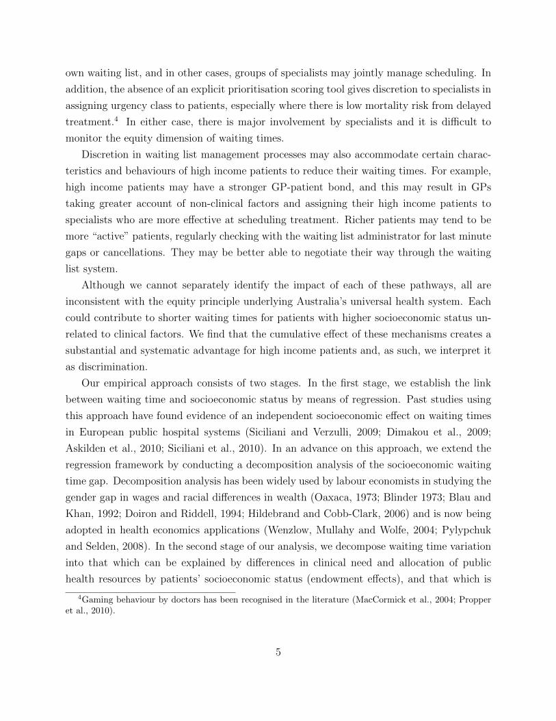
monitor the equity dimension of waiting times.
Discretion in waiting list management processes may also accommodate certain charac-
teristics and behaviours of high income patients to reduce their waiting times. For example,
high income patients may have a stronger GP-patient bond, and this may result in GPs
taking greater account of non-clinical factors and assigning their high income patients to
specialists who are more effective at scheduling treatment. Richer patients may tend to be
more “active” patients, regularly checking with the waiting list administrator for last minute
gaps or cancellations. They may be better able to negotiate their way through the waiting
list system.
Although we cannot separately identify the impact of each of these pathways, all are
inconsistent with the equity principle underlying Australia’s universal health system. Each
could contribute to shorter waiting times for patients with higher socioeconomic status un-
related to clinical factors. We find that the cumulative effect of these mechanisms creates a
substantial and systematic advantage for high income patients and, as such, we interpret it
as discrimination.
Our empirical approach consists of two stages. In the first stage, we establish the link
between waiting time and socioeconomic status by means of regression. Past studies using
this approach have found evidence of an independent socioeconomic effect on waiting times
in European public hospital systems (Siciliani and Verzulli, 2009; Dimakou et al., 2009;
Askilden et al., 2010; Siciliani et al., 2010). In an advance on this approach, we extend the
regression framework by conducting a decomposition analysis of the socioeconomic waiting
time gap. Decomposition analysis has been widely used by labour economists in studying the
gender gap in wages and racial differences in wealth (Oaxaca, 1973; Blinder 1973; Blau and
Khan, 1992; Doiron and Riddell, 1994; Hildebrand and Cobb-Clark, 2006) and is now being
adopted in health economics applications (Wenzlow, Mullahy and Wolfe, 2004; Pylypchuk
and Selden, 2008). In the second stage of our analysis, we decompose waiting time variation
into that which can be explained by differences in clinical need and allocation of public
health resources by patients’ socioeconomic status (endowment effects), and that which is
4Gaming behaviour by doctors has been recognised in the literature (MacCormick et al., 2004; Propperet al., 2010).
5

due to differences in the return to these characteristics in terms of reduced waiting times
(treatment effects). We employ the approach proposed by Firpo, Fortin and Lemieux (2007,
2009) which allows the endowment and treatment effects to vary across the waiting time
distribution. Having a flexible approach is important because the endowment and treatment
effects may be stronger at different parts of the distribution. For example, preferential
treatment to patients on the basis of their socioeconomic status may be more likely to occur
if there is lower mortality risk, so we might expect stronger preferential treatment on the
basis of socioeconomic status in the upper tail of the waiting time distribution.
We find evidence of prioritisation of the most socioeconomically advantaged patients at
all quantiles of the waiting time distribution. At the 90th percentile of the waiting time
distribution, the least socioeconomically advantaged patients wait over 4 months longer for
an elective procedure compared to the most advantaged patient group. None of this gap
can be attributed to differences in clinical needs. About a third of it can be attributed to
favourable treatment of the most socioeconomically advantaged patients and the remaining
gap is due to supply-side endowments that work in their favour. Our results suggest that
the burden of long waits falls disproportionately on the least socioeconomically advantaged
patients and that the current waiting list operation in Australia falls short of the policy goal
of equity.
2 Data
Our data are derived from administrative records of completed waiting list episodes during
the period 2004-2005 in public hospitals in the state of New South Wales (NSW), the most
populous state of Australia. This data set contains information on urgency category, patient’s
age, gender, detailed chronic conditions (diagnoses), procedures and postcode of residence.
We focus on NSW residents and public hospitals that treat acute illnesses. This excludes
smaller health facilities, such as small non-acute hospitals, hospices, multi-purpose units and
rehabilitation units. Further, we consider only patients who have spent at least a day on the
waiting list because patients with zero waiting days are likely to represent quasi emergency
admissions especially in areas with no emergency departments.5 We do not have reliable
information on private health insurance status, however previous studies suggest that those
without private health insurance are much more likely to use the public system than those
privately insured (Savage and Wright, 2003).
5Patients with zero waiting days make up 5% of admissions.
6

We make two more restrictions to get a clearer interpretation of the socioeconomic gap in
waiting time. First, as mentioned, we include only non-charge or public patients6 who make
up the vast majority of admissions to public hospitals (87%). Second, we focus on patients
who live in the state capital, Sydney, who have similar geographic access to public hospitals.
The final sample size consists of 90,162 patients.
As with most, if not all, registry data, information on personal income is not available.
We therefore use information on patients’ residential postcode to combine the individual
patient clinical data with census data on socioeconomic status. The Australian Bureau
of Statistics (ABS) constructs a number of summary measures of economic advantage and
disadvantage, known as SEIFA (Socio-Economic Indexes for Areas) indices, for geographic
areas (ABS, 2001). We use the Index of Relative Advantage and Disadvantage. This index
is constructed using a list of socioeconomic measures such as income, education, employ-
ment status and housing characteristics. The score underlying the index is given by the
first principal component in a principal component analysis; it is the single variable that
best summarises the common relationship among the above set of socioeconomic indicators.
Areas are then ordered according to their scores, and the Index of Relative Advantage and
Disadvantage is the decile of the score for that area (i.e. 1, 2, ... 10). An area with a high
index has a relatively high incidence of advantage and a relatively low incidence of disadvan-
tage. We re-group the deciles into quintiles, SEIFA 1 to 5, and interpret the bottom 20%,
SEIFA 1, as the least socioeconomically advantaged group and the top 20%, SEIFA 5, as the
most advantaged group. To give an idea of the income disparities across the SEIFA groups,
the median individual income of the most advantaged group is about 1.4, 1.7, 2.0 and 2.2
times greater than that of SEIFA 4, 3, 2 and 1, respectively.7
It is possible that the socioeconomic gap in waiting time is not due to discrimination
per se, but because better-off individuals tend to live in areas with a greater supply of
hospital services. Therefore, we also control for a rich set of hospital supply measures. We
supplement patient-level data with information on hospital characteristics obtained from
the NSW Health Services Comparison Data Book(s). The books contain detailed in-hospital
information including activity level, expenditures and staffing. We use the 1997-1998 and
2007-2008 data, which are the closest available books to our sample period. For each variable
of interest, we take the average values from the two periods. We tested the sensitivity of
6These are Medicare-eligible, public patients excluding Veteran’s Affairs, Defence Forces and Worker’sCompensation patients.
7Results using only the median household income to define economically advantaged or disadvantagedgroups are qualitatively the same. They are available from authors upon request.
7

our results to using a weight of 0.3 for 1997-1998 and a weight of 0.7 for 2007-2008, but
the weighting rule does not substantially alter the results. This indicates that hospital
characteristics tend to change slowly.
We consider the following supply variables: (i) to capture the potential bed competition
with admissions from emergency departments we use admission from emergency as a propor-
tion of total admissions; (ii) to measure activity we use same day admissions as proportion
of total admissions and the bed occupancy rate; (iii) to measure the share of private (paying)
patients we use private beds as a proportion of occupied beds; (iv) to capture complexity
we use average length of stay of acute episodes; and (v) to measure human resources we use
inpatient clinical equivalent full-time staff per available bed and the shares of total hospi-
tal expenses of medical salaries and visiting medical officer (VMO) payments and nursing
salaries. The supply variables are entered as deviations from the overall sample mean. This
is done to aid the interpretation of results.
The means of waiting times and some explanatory variables by SEIFA are presented in
Table 1.8 Across SEIFA groups, the most socioeconomically advantaged patients (SEIFA 5)
are older and assigned more urgent categories. Their mean waiting time is markedly shorter
than that of other patients (74 days compared with 112 days for the least socioeconomically
advantaged patients (SEIFA 1)). Because the distribution of waiting time is positively
skewed, for estimation we use the log of waiting time.
A potential source of bias in the data is that we do not observe patients who choose to
be treated at private hospitals. To the extent that the choice of a private hospital is more
likely to be exercised by socioeconomically advantaged patients with long expected waits,
this may lead to underestimation of their average waiting times. If they are non-urgent
and tend to elect for private hospital admission, we would expect to observe a substantially
lower share of most socioeconomically advantaged in the 365 day urgency class than for lower
socioeconomic groups. We do not have data on private hospital admissions, however, we do
observe a considerable share of the most socioeconomically advantaged patients in the least
urgent class (see Table 1). This suggests that any bias due to selection of socioeconomically
advantaged patients with long expected waits into private hospitals is likely to be minimal.
With regard to supply characteristics, SEIFA 5 patients are treated in hospitals with
higher levels of all supply variables apart from medical staffing cost shares. Noticeably, they
use hospitals with a high share of private bed days whilst the opposite is true for the SEIFA
8For conciseness, we suppressed the summary statistics related to diagnoses. They are represented by 28dummy variables. The number of conditions are based on conditions which are associated with hospitalisation(e.g., short-sightedness is excluded).
8

1 patients.
Table 1: Variable means by SEIFA quintile
3 Estimation
3.1 Oaxaca and Blinder decomposition
To quantify the role of various factors in driving the observed socioeconomic waiting time
gap, we undertake a decomposition analysis that has been extensively used in the labour
economics literature. Seminal papers of Oaxaca (1973) and Blinder (1973) (here onwards
OB) decompose gender gap in wages into the contribution of human capital, job types and
industry, other demographics, and interpret the contribution of unexplained factors as a
discrimination effect.
The OB decomposition takes advantage of a linear regression model to decompose the
expected outcomes of any two distinct groups, A and B. Let W be waiting time and X be
a row vector of K individual covariates. The conditional mean of W for group j (j = A,B)
is E(W |X, J = j) = E(X|J = j)βj where E(X|J = j) is the mean of X among group j,
and is a [Kx1] vector of regression coefficients, which can be estimated by OLS. The OB
approach would decompose the overall difference in mean waiting times into two components:
‘endowment’, which measures how waiting time setting factors are unequally distributed
across groups, and ‘treatment’, which relates to differences in coefficients applied to different
groups. By adding and subtracting a counterfactual conditional mean, for instance E(X|J =
A)βB, which reflects a situation in which group B individuals have the covariates of group
A, it is possible to identify the two components:
∆µ = µA − µB= E(X|J = A)βA − E(X|J = B)βB + E(X|J = A)βB − E(X|J = A)βB
= (E(X|J = A)− E(X|J = B))βB + E(X|J = A)(βA − βB) (1)
≡ ∆µE + ∆µ
T ,
where ∆µ, ∆µE and ∆µ
T denote the overall difference in means, the difference in means due to
endowment and the difference in means due to differences in β or ‘treatment’, respectively.
The latter is the unexplained part of the socioeconomic waiting time gap.
9

Moreover, the additivity assumption allows identification of the contribution of each
covariate to the endowment and treatment component. Rewriting equation (1) and replacing
it with its sample counterparts, we have
∆̂µ = WA−WB =∑k
(XAk−XBk)β̂Bk +∑k
XAk(β̂Ak− β̂Bk) + (α̂A− α̂B) = ∆̂µE + ∆̂µ
T , (2)
where WA and WB are sample mean waiting times for group A and B, respectively, β̂jk is
the OLS slope estimate for variable Xk (k = 1, ..., K) for group j, Xjk is its corresponding
sample mean, and α̂j is the intercept. Throughout this study, we define group B as the most
socioeconomically advantaged group, SEIFA 5.
We partition Xk into two sets. The first set reflects clinical need and consists of patient’s
age, gender, procedure, chronic diagnoses, number of chronic diagnoses and urgency assign-
ment. The second set consists of the supply characteristics mentioned above. With two sets
of waiting time determinants, the socioeconomic waiting time variations can be attributed to
4 sources: (i) an endowment effect associated with patients’ clinical needs; (ii) an endowment
effect associated with supply characteristics; (iii) a treatment effect associated with patients’
characteristics; and (iv) a treatment effect associated with supply characteristics.
We argue that (ii)−(iv) have interpretations as discrimination. Discrimination associ-
ated with patients’ health endowments can be explained by the behaviour of the providers
responsible for scheduling procedures. For example, being assigned an urgency classification
of 365 days results in a longer waiting time for SEIFA 1 patients compared with SEIFA
5 patients. Meanwhile, discrimination related to supply in a universal health care system
can take two forms: unequal access to public hospital resources and differential impacts of
hospital resources by socioeconomic status. The former reflects a very broad dimension of
discrimination extending beyond the behaviour of doctors or hospitals. It partly reflects
the allocation procedure that assigns patients to specialists and hospitals but also access to
transport and information about alternative hospitals.
We attribute differences in intercepts (α̂A − α̂B) in equation (2) to patient treatment
effects. The intercept has an interpretation of the expected waiting time of the omitted
patient group in an average hospital. The differences in intercepts can reflect (a) unmeasured
clinical need; (b) the ability of patient to negotiate the system; (c) unmeasured hospital
characteristics (eg quality of hospital management); or (d) pure discrimination effects. We
have detailed data on patient diagnoses and procedures that it is unlikely that differences
in the intercept reflect unmeasured clinical need. Once we rule out (a), we are left with (b),
10

(c) and (d) all of which can have interpretations as discrimination.
While the OB approach is popular and has intuitive appeal, it suffers from several well-
recognised drawbacks. OB focus on the mean but it is quite possible, for example, that
waiting time gaps are larger in the upper tail of the waiting time distribution because pa-
tients’ conditions are less urgent with lower mortality risk of delayed treatment. Another
potential bias comes from the fact that OLS coefficients β depend on the distribution of
covariates. This means that when they are estimated for different groups, the difference be-
tween them can be an empirical manifestation of the different covariate distributions between
groups, rather than reflecting the true differences in treatment effects.
DiNardo, Fortin and Lemieux (1996) and Firpo, Fortin and Lemieux (2007; 2009) (here
onwards FFL) propose a more flexible method of decomposition analysis that generalises
the OB approach by allowing OB-type decomposition of any characteristic of a distribution
(e.g. variance, quantiles, etc.). The FFL method consists of two stages. In the first stage a
counterfactual distribution of waiting time is constructed using a matching technique. The
counterfactual distribution is the distribution which would have prevailed under the waiting
time generating process for SEIFA 5 patients (group B) but with the characteristics of less
socioeconomically advantaged patients (group A). This stage, as proposed in DiNardo et al,
removes waiting time differentials due to differences in the distribution of covariates between
the two groups by reweighting observations in group B. In particular, for each comparison
group A, we estimate a weighting function to construct a counterfactual distribution of
waiting time for SEIFA 5 patients when they are assigned characteristics of group A. The
weights are estimated using a logit model predicting group A membership as a function of all
patient and supply characteristics.9 There are four counterfactual distributions for SEIFA 1
to 4 with the SEIFA 5 waiting time distribution. In each comparison pair, the counterfactual
group is called group C.
In the second stage of FFL decomposition these counterfactual distributions are used to
compute treatment and endowment effects for selected characteristics of the waiting time
distribution (i.e. quantiles in our study) and to decompose these effects into contributions
of various characteristics (i.e. patient and supply characteristics) using re-centred influence
function (RIF) regressions. Next section will discuss the second stage of FFL decomposition
in detail.
9Details of the weighting function can be found in DiNardo, Fortin and Lemieux (1996). Based on thelogit estimates, we can find weights on observations that equalise the patient and supply characteristicsacross groups (so SEIFA group is the only difference).
11

3.2 FFL decomposition
Unlike the mean, which can be decomposed using OLS (as in OB), we cannot decompose
quantiles using the standard quantile regressions. The coefficients in OLS indicate the effect
of covariates X on the conditional mean E(W |X) in the model E(W |X) = Xβ. This yields
an unconditional mean interpretation where β can be interpreted as the effect of increasing
the mean value of X on the (unconditional) mean value of W .
By contrast, only the conditional quantile interpretation is valid in the case of quantile
regressions. A quantile regression model for the τ th conditional quantile postulates that
qτ (X) = Xβτ . By analogy with the case of the mean, βτ can be interpreted as the effect of
X on the τ th conditional quantile of W given X. However, the law of iterated expectations
does not apply in the case of quantiles so, qτ 6= EX [qτ (X)] = E(X)βτ , where qτ is the
unconditional quantile. It follows that βτ cannot be interpreted as the effect of increasing
the mean value of X on the unconditional quantile . This greatly limits the usefulness of
quantile regressions in decomposition problems.
FFL suggest estimating the recentered influence function (RIF) for quantiles of waiting
times and then conducting the OB-style decomposition exercise using the RIF regression
coefficients. Consider the influence function IF (w; v) which measures how much influence
an observation w has on the distributional statistic of interest v, such as a quantile. The RIF
is defined as RIF (w; v) = v(FW ) + IF (w; v), where FW is the waiting time distribution. By
definition, the expectation of the IF with respect to the distribution of w is equal to zero.
Hence, the expectation of the RIF is equal to the statistic of interest.
It can be shown that for observation w the RIF for quantile qτ has the form:
RIF (w; qτ ) = qτ +τ − ι{w ≤ qτ}
fW (qτ ), (3)
where the second term is the IF, qτ is the τ th percentile of waiting time, ι{.} is an indicator
function for waiting time up to and inclusive of the τ th percentile and fW (qτ ) is the density of
W evaluated at qτ . The RIF function can be computed for each observation w (after replacing
fW (qτ ) with its kernel density estimate), and the conditional (on X) expectation of the RIF
can be estimated by OLS regression in which the RIF acts as a dependent variable. The
estimated coefficients γ from the RIF regression can be interpreted as the effect of increasing
the mean value of X on the unconditional quantile qτ (using FFL’s terminology, measures
the ‘unconditional quantile partial effect’).
To save notation, let vA,vB and vC be the quantile of interest for groups A, B and a
12

counterfactual group C, respectively. Recall that the expectation of the RIF is equal to the
statistic of interest. Hence in the presence of covariates we can apply the law of iterated
expectations to write
vj = E(RIF (wj; vj)|J = j) = EX{E(RIF (wj; vj)|X, J = j)} for j = A,B
and
vC = E(RIF (wB; vC)|J = A) = EX{E(RIF (wB; vC)|X, J = A)},
where the notation wj means that observation w belongs to group j.
To allow direct comparison with the OB approach, suppose that the conditional (on
X) expectation of the RIF can be well approximated by a linear function of covariates as
in OB, i.e. E(RIF (wj; vj)|X, J = j) ≈ (X|J = j)γvj , where γvj are the RIF regression
coefficients. Then the unconditional quantile vj is the expectation of (X|J = j)γvj with
respect to X|J = j and thus can be represented as a product of E(X|J = j) and γvj :
vj ≈ E(X|J = j)γvj and vC ≈ E(X|J = A)γvC . (4)
With this approximation, it follows that the endowment and treatment components can be
written as:
∆vE = vC − vB = E(X|J = A)γvC − E(X|J = B)γvB
∆vT = vA − vC = E(X|J = A)γvA − E(X|J = A)γvC (5)
We can write a version of equation (2) for quantile of interest v as:
∆̂vE =
∑k
XCAkγ̂
vCk −
∑k
XBkγ̂vBk =
∑k
(XCAk −XBk)γ̂
vBk + R̂v
1
∆̂vT =
∑k
XAk(γ̂vAk − γ̂vCk) + R̂v
2, (6)
where XCAk is the sample mean of variable Xk in the SEIFA 5 sample, weighted using the
characteristics of group A, R̂v1 =
∑kXAk(γ̂
vCk − γ̂vBk) and R̂v
2 =∑k γ̂
vCk(XAk −X
CAk). Com-
pared to equation (1), apart from R̂v1, ∆̂v
E is similar to the OB endowment component, while
∆̂vT resembles the OB treatment component but with γ̂vCk instead of γ̂vBk. So for the treat-
ment effect, we are using group C as the reference group, instead of group B. This minimises
potential bias in the treatment effect due to the distinct distribution of covariates between
13

groups. R̂v1 can be interpreted as an error associated with the fact that a potentially incor-
rect specification may be used for the RIF regression (Firpo et al., 2007). Meanwhile, R̂v2
measures the appropriateness of the weighting function. If the weighting function is valid,
R̂v2 should be small.
It is noteworthy that because FFL is based on linear regressions like OB, the FFL ap-
proach is path independent, that is, the order in which the different elements of the detailed
decomposition are computed does not affect the results of the decomposition. This contrasts
with the DiNardo et al.’s reweighting approach, which is path dependent. In estimation, we
take the natural logarithm of waiting times, which are highly positively skewed. The RIF
is computed following Fortin’s (2009) sample code and given the RIF regression results, the
decomposition exercise is implemented using oaxaca command in STATA (Jann, 2008).
4 Results
4.1 Regression results
Before we proceed to the decomposition results, we confirm that socioeconomic status has
independent effects on waiting time by running a linear regression. Table 2 reports the results
of two regression models that differ in the sets of covariates included. Model 1 includes only
clinical needs and SEIFA groups while Model 2 also includes supply factors. In both models,
the coefficients on SEIFA categories are jointly significant at the 1% level (F-statistics of
140 and 92 for Model 1 to 2, respectively). Socioeconomic groups have significant and
independent effects on waiting time. When controlling only for clinical need (Model 1),
relative to SEIFA 5 patients, SEIFA 1-3 patients wait on average 30% longer (about 28 days
at the overall mean waiting time of 94 days) and SEIFA 4 patients wait 19% longer (18
days).
When both patient and supply characteristics are added in Model 2, the socioeconomic
waiting time gaps are narrowed compared to those found in Model 1. However, the estimates
still imply that the lower socioeconomic groups wait 16-24% longer than SEIFA 5 patients,
depending on the SEIFA group. If health resources reduce waiting times, this upward bias
suggests a positive relationship between supply and socioeconomic status. Supply consists
of several measures and they have differing effects on waiting times. Waiting times increase
with emergency admissions, bed occupancy rates and share of hospital expenditure to pay
for medical staff and visiting medical officers (VMO). However, waiting times decrease with
the proportion of private patients, the average length of stay, the staffing level per bed and
14

the nursing share in total hospital expenditure.
Table 2: Regression results of log waiting time
4.2 Distribution of log waiting times
Figure 1 plots kernel density estimates of log waiting times by socioeconomic status. It
is clear that a greater mass of SEIFA 5 waiting times is concentrated in the lower half
of the distribution compared with other patients. This implies that the share of patients
experiencing extensive delays is lower for SEIFA 5 patients than for any other patient group.
The upper tail is the thickest for the two lowest SEIFA groups. The noticeable hump at
zero is explained by the presence of patients who are on the waiting list for just a day before
they are admitted. SEIFA 5 has a higher share of these one-day patients than other SEIFA
groups.
Figure 2 shows the density of counterfactual waiting time for SEIFA 5 patients for each
comparison pair (the first stage of the FFL approach). Recall that the counterfactual waiting
time reflects the waiting time that would occur had SEIFA 5 patients had the covariates of
less socioeconomically advantaged patients. We can see that at the lower tail of the waiting
time distribution (short waits), the counterfactual distribution drifts somewhat from the
actual waiting time distribution of SEIFA 5 towards that of the less advantaged patients
suggesting that covariates have a lot to do with socioeconomic waiting time gaps for short
waits. At the upper tail of the waiting time distribution (long waits), the counterfactual
distribution approaches the waiting time distribution of less advantaged patients but the
relatively large remaining gap suggests that factors other than the distribution of covariates
are important in driving the socioeconomic waiting time gaps for long waits.
Figure 1: Density of log waiting times
Figure 2: Density of actual and counterfactual log waiting time by SEIFA pair
4.3 FFL Results
From equation (3), for each patient, we compute the RIF (wj; qj,τ ) using an estimate of qτ
from each group in the pairwise sample. f(qτ ) is estimated by an Epanechnikov kernel with a
15

bandwidth of 0.12.10 We decompose the waiting time gap for 9 waiting time quantiles, from
the 10th to the 90th) quantile. However, for reporting purposes, we report the results for only
3 quantiles, Q10, Q50 (the median) and Q90. We will first discuss the decomposition results
for overall patient and supply characteristics. Later, we present the results of a detailed
decomposition of supply characteristics.
4.3.1 Decomposition of overall patient and supply characteristics
Table 3 reports the total endowment and treatment effects for patient and supply character-
istics, as well as the total differences in log waiting times and residuals. The first two rows
assure us that the observed log waiting time gap and the estimated RIF gap (equation (5))
are very close. In general, waiting time gaps are large and do not decrease in high waiting
time quantiles. At the bottom of the waiting time distribution, a 65% (exp(0.5055)-1) wait-
ing time difference translates to 2 days, but at the top of the distribution, a 65% waiting
time difference means that the most socioeconomically advantaged patients are admitted
over 4 months earlier than the least advantaged patients. This is a substantial delay which
can be costly to patients (e.g. declining work ability and prolonged inconvenience). The last
two rows in Table 3 report the size of the residuals in equation (6). In general, they are
relatively small, lending support to the use of the FFL approach. R̂v1, which can be seen as
an adjustment factor to the endowment effect in the case where the linear specification is
inaccurate, tends to be negative at short waits and positive at long waits.11 Since we observe
that the most socioeconomically advantaged patients access better health resources (Table
1), the positive adjustment factor may reflect a flatter relationship between waiting times
and supply as supply gets larger. Meanwhile, R̂v2 reveals no noticeable pattern and is mostly
insignificant.
Table 3: Decomposition of overall patient and supply characteristics
A striking feature of Table 3 is that in the comparisons between SEIFA 5 and each of
the less advantaged groups the patient endowment effect is an important factor only at low
waiting times and that its importance declines markedly as waiting time increases to become
10We experimented with different bandwidths and Gaussian weights and our results are robust to thesealternative specifications.
11In the labour literature where the decomposition exercise often focuses on the evolution of wage gaps,residuals are often found to be small. This is because groups are defined by time and group membership iswell predicted by covariates such as age and the unemployment rate.
16

approximately zero at Q90. For short waits, a substantial part of the socioeconomic waiting
time gap can be explained by less advantaged patients’ health characteristics. At Q10 patient
endowments explain 35% (0.1784/0.5055) and 33% (0.2108/0.6378) of the waiting time gap
with SEIFA 1 and 2 patients, respectively, and about a half of the waiting time gap with
SEIFA 3 and 4 patients. However, at Q90, surprisingly the endowments of the better-off
patients tend to make them wait longer, but the effects are trivially small except for the
comparison with SEIFA 3.
The endowment effect associated with supply characteristics is positive in all quantiles
of the waiting time distribution. This indicates that differential public health resource avail-
ability by socioeconomic status contributes to the waiting time differential. The supply
endowment effect gets larger at the top of the waiting time distribution. For SEIFA 1 to
3, it explains the bulk of the socioeconomic waiting time gap. For SEIFA 4, the supply
endowment effect is significant, but is not the dominant source of the waiting time gap. This
exception suggests that public health resource availability is relatively similar for the 40%
of the most socioeconomically advantaged patients.
The patient treatment effect behaves very differently from the patient endowment effect:
it is positive and dominates at the top of the waiting time distribution. The positive patient
treatment effect indicates discrimination in favour of the most socioeconomically advantaged
patients. At Q90, the size of the discrimination ranges from 33% to 54% (for the natural log
of the waiting times), which translates to 30 to 60 days.12 Of the four aggregate effects, the
supply treatment effect is relatively small and not generally significant.
Figure 3 depicts the size of the four aggregate effects across 9 waiting time quantiles. The
patient and supply endowment effects are equal at Q60 (Q70 for SEIFA 2 patients) as the
latter assumes a greater role in explaining gap in long waits. The patient treatment effect
is relatively flat, except for SEIFA 4, where it steepens post-median. The patient treatment
effect dominates the patient endowment effect post-median for SEIFA 1, but more quickly
for other comparison groups. Lastly, as discussed, the supply treatment effect is flat around
zero (except at the middle of distribution for SEIFA 1).
12The shares are the ratios of the patient treatment effects to the overall differences in Q90 of the naturallog of waiting times between SEIFA groups 1-4 and SEIFA group 5. To obtain the results in days, note thatfrom (6) the relationship between the quantiles of waiting times in levels, qj ≡ e(vj) for j = A,B, is givenby qA ≈ qB · epe · ese · ept · est, where pe, se, pt and st denote patient and supply endowment and patientand supply treatment effects for logs, respectively. The contribution of each factor to the difference betweenqA and qB is not path independent in the sense that this contribution depends on the order in which thefactor-specific rate of change is applied to the quantile qB of the baseline group. To estimate the size of it’scontribution in days, we apply the patient treatment effect first. For example, for the SEIFA group 1 thecontribution of the patient treatment in days is computed as 197 · (e0.17 − 1) = 37 days.
17

In general, the patient treatment effect and the supply endowment effect (both of which
we interpret as discrimination) account for the bulk in of the waiting time gap in long waits
especially at Q90. While their relative sizes vary across the distribution their combined
effect explains most of the difference in waiting time. For short to median waits, the patient
endowment effect is also an important factor
Figure 3: Aggregate endowment and treatment effects
4.3.2 Detailed decomposition of supply factors
In this section, we conduct detailed decomposition of supply factors to get more information
about public health resource use and public hospital operation. From a policy perspective,
supply factors are potential policy instruments and targets. Figure 4 plots the RIF regression
coefficients of supply variables in the SEIFA 5 sample at each waiting time quantile, γ̂vBk.13
These coefficients are used to compute the supply endowment effect (see equation (6)).
Figure 4: RIF regression coefficients for SEIFA 5 patients
Four of the eight supply variables have changing signs along the waiting time distribution.
This highlights the importance of analysis beyond the means. The rate of admissions from
an emergency department (ED) has a negative impact on waiting times. This result is
surprising since we expect an increase in emergency admission rate to delay the admission of
non-emergency procedures to manage bed occupancy. Unlike demand for elective surgeries,
arguably hospitals have less control over emergency admissions. Reconciling this result with
other SEIFA groups, we find that this negative effect is unique to SEIFA 5 patients. The
waiting times of patients in SEIFAs 1 to 4 increase with admission rates of ED patients.
A higher proportion of same day admissions and clinical full-time staff are associated
with shorter waiting times except at the bottom of the waiting time distribution (Q10).
On the other hand, bed occupancy rates, which measure hospital activity, tend to increase
waiting time, as do medical staff and visiting medical officers (VMOs). These two results
may capture long waiting lists in large teaching hospitals (e.g. Principal Referral hospitals).
The share of private activity increases the waiting time at low quantiles but reduces
waiting time at high quantiles. This suggests that the most socioeconomically advantaged
patients who are waiting for least urgent procedures like cataract and knee replacements
13For conciseness, the full RIF regression coefficients are not reported but are available from the authorsupon request.
18

(i.e. those at the top quantiles) benefit from being treated at hospitals with high share of
private activities. Put another way, this result hints at a positive association between the
socioeconomic status of public patients and the share of private patients in the hospitals they
attend. The most socioeconomically advantaged public patients are more likely than others
to be admitted as private patients. Public hospitals in Australia operate under fixed budgets,
and increasing the share of privately financed hospital activities is one of the few ways they
can generate additional revenues. There is some evidence that public hospitals have been
increasing efforts to boost their private revenues (Private Health Insurance Administration
Council, 2006).
The upper panel of Table 4 reports endowment effects for each supply variable. ED and
complexity contribute positively to waiting time gaps at any point of the distribution. Given
that these two variables shorten waiting times, their inequality-enhancing effect implies that
the most socioeconomically advantaged patients access hospitals with higher ED rates and
complexity. In contrast, bed occupancy rates have a global negative effect, but relatively
small in size. Given that bed occupancy rates increase waiting time, its inequality-reducing
effect implies that the most socioeconomically advantaged patients tend to be treated in
hospitals with high bed occupancy rates. All in all, these results suggest that the most
socioeconomically advantaged patients access large hospitals which have busy ED and treat
complex cases.
Table 4: Detailed decomposition of supply characteristics
Other supply variables have changing signs along the waiting time quantiles. The pro-
portion of same day admissions and fulltime staff ratios widen the waiting time gap at Q10
but narrow it elsewhere. Spending on medical and nursing staff reduce waiting time gaps at
Q90. A policy implication of the negative effect of these variables is that a reduction in the
waiting time gap can be promoted by more equal access to hospital medical professionals.
The endowment effect due to private activity is negative at the lower half of the waiting
time distribution and positive at high waiting time quantiles. It dominates the supply
endowment effect at Q90, mitigating the inequality-reducing effects of some of the other
supply variables. The most socioeconomically advantaged patients tend to use hospitals
with high private activity. Those who are waiting for less urgent procedures (long waits)
benefit from this higher share of private activities in the form of shorter waiting times. The
impact of the proportion of private patients is comparable in size to the overall patient
treatment effect. It explains 35%, 28%, 52% and 27% of waiting time gap (in logs) with
19

SEIFA 1, 2, 3, and 4, respectively, which translates to earlier admissions of SEIFA 5 patients
by 22 to 48 days. ED and Complexity add to the waiting time gap at this point.
The lower panel of Table 4 reports the supply treatment effects. Many of these lack
statistical significance. The treatment effects associated with ED, Bed, Doctors and Staff are
generally smaller than their respective endowment effects. The aggregate supply treatment
effect is driven mainly by the proportion of private beds and complexity. Complexity tends to
reduce waiting time inequality. This may suggest that when hospitals are more advanced (as
measured by complexity), they benefit less advantaged patients more. In contrast, private
activity has a sizeable positive effect at the median for SEIFA 1. This explains the hump
in the aggregate supply treatment effect we saw earlier in Figure 3. A positive treatment
effect associated with private activity suggests that hospitals give the most socioeconomically
advantaged patients priority when faced with increased private activity. At the middle of the
distribution, such preferential treatment is likely to affect mid-urgent patients whose target
waiting times are between 30 to 90 days.
In summary, the socioeconomic waiting time gap is driven by both patient and supply
factors. The most socioeconomically advantaged patients are prioritised in the waiting list
despite having similar clinical needs to other patients. This source of discrimination is ob-
served in almost all points of the waiting time distribution, meaning even urgent patients are
affected. Socioeconomically advantaged patients benefit from higher private activity in the
hospitals they attend. In contrast less advantaged patients may be delayed to accommodate
admissions of ED patients and private patients in hospitals with low private revenues.
4.3.3 Robustness of the patient treatment effect
We conduct several robustness checks. First, to entertain the possibility more socioeconom-
ically advantaged patients are more informed about waiting times and travel to hospitals
with the shortest waiting times, we include distance to hospital as part of patient character-
istics. We use the haversine formula for computing great-circle distances between the centre
point of the postcode where the patient lives and the location of the treating hospital. The
mean distance ranges from 9.5 to 14.6 kilometers across SEIFA groups. Row 1 of Table 5
reproduces the results for patient treatment effects from Table 3 and the results including
distance as a patient characteristic are reported in row 2. It can be seen that the patient
treatment effects remain positive and significant, and are even larger in the comparisons with
the lowest two SEIFA groups.
Second, if privately insured patients, who expect a long wait in public hospitals, substitute
20

to private treatment, we may overestimate the socioeconomic waiting time gap at the upper
tail of the distribution. We do not have reliable insurance information at the patient level.
As a proxy, we include the proportion of households with private insurance at the postcode
level as a patient characteristic. The mean insurance rate is increasing with socioeconomic
status, from 42% for SEIFA 1 to 69% for SEIFA 5. Row 3 of Table 5 shows that patient
treatment effects at long waits are largely unchanged.
Third, another test of substitution to private hospitals is to repeat the analysis excluding
procedures that are predominantly undertaken in private hospitals. Of procedures on eye and
adnexa and ear, nose and throat (ENT), 67% are performed in private hospitals (AIHW,
2006). In the sample we find that ophthalmology and ENT specialties have the longest
average public hospital waiting times (213 and 202 days, respectively). These long expected
waits may motivate more socioeconomically advantaged patients to choose private hospitals
where waiting times are negligible. As a sensitivity test we exclude patients in the two
specialties from the sample. This reduces the sample to 69,425 (77%). Row 4 of Table 5
reports patient treatment effects from the restricted sample. At long waits, we find patient
treatment effects are larger, except in the comparison with SEIFA 3.
Fourth, our analysis implicitly assumes within-SEIFA variation is negligible. To reduce
within-group income variation which may contaminate comparisons across groups, we focus
on postcodes within a SEIFA group have ”similar” income. We take the median household
income from Census data for each postcode and calculate the mean and standard deviation
for each SEIFA group. In each SEIFA group we select only postcodes which are within one
standard deviation away from the mean.14 Row 5 of Table 5 row shows the re-estimated
patient treatment effects remain significant and are largely unchanged.
Fifth, the literature from the US finds evidence of differences in health care utilisation
based on race/ethnicity and language barriers, which may also be linked to socio-economic
status (e.g., Yoo et al., 2009; Leighton and Flores, 2005; Fiscella et al, 2005). The US
health care market is privately driven, so access is contingent on ability-to-pay. In contrast,
Australia has a public health system (Medicare) which guarantees access to free public
hospital treatment for all residents. Our analysis includes only Medicare eligible patients.
We do not have information about ethnicity however we know country of birth and that
14For SEIFA 1 and SEIFA 5, we place one-sided restrictions, excluding postcodes with medians above onestandard deviation of the mean for SEIFA 1 and below one standard deviation of the mean for SEIFA 5. Forthe other SEIFA groups we place two-sided restrictions. This reduces the sample to 80,398 (89% of originalsample); the new samples for SEIFA 1 to 5 are 6,864 (88%), 8,960 (89%), 15,315 (87%), 23,998 (86%) and25,261 (95%), respectively.
21

98% of the sample is non-indigenous (Aboriginal or Torres Straits Island) patients. To test
the sensitivity to indigenous status and being foreign born, we conduct a robustness check
excluding indigenous patients, those born overseas and those whose main language is not
English. The sample size is reduced to 58,572 (65% of the original sample). Row 6 Table 5
reports the patient treatment effects, which are consistent with the main results.
Sixth, we restrict the sample to Sydney patients. The restriction was primarily to ensure
patient access to large public hospitals. Furthermore, some areas outside Sydney border
other states and patients who seek treatment interstate are missing from our data. Because
Australian public hospitals are managed by state governments, there can be state variations
in policies and waiting times, so including border regions may induce sample selection bias
by omitting patients who face shorter waits in different states. We test the sensitivity of
the results by adding non-border regions with major cities to the Sydney sample. Row
7 of Table 5 reports the patient treatment effects for this sample. The result of positive
patient treatment effects across the waiting time distribution is robust to the new sample.
However, the impact of socioeconomic status is larger in the upper tail of the distribution
(long waits). This is consistent with the inclusion of regions outside Sydney which have
higher concentrations of retirees with chronic conditions requiring non-urgent treatment.
Table 5: Robustness of patient treatment effect
5 Conclusion
Waiting time is the rationing device used to equate supply and demand of non-emergency
procedures in public hospital systems where treatment is free at the point of care. Equitable
access to care requires that the length of time to treatment should solely reflect patients’
clinical needs. Extended delays in receiving treatment have been found to prolong suffering,
decrease earning capacity and cause deterioration of quality of life (Oudoff et al. 2007; Hodge
et al. 2007).
Using the case of public (non-paying) patients in Australian public hospitals, we find that
waiting times are strongly influenced by patients’ socioeconomic status. While we are unable
to identify the exact mechanism(s) driving lower waiting times for the most advantaged
patients, which could be multiple and interrelated, it is clear that it is not determined
by clinical need. In accordance with the equity principle of universal health systems, we
interpreted the gap not attributable to clinical factors as discrimination. We find that the
22

largest contributor to discrimination is favourable treatment given to the most advantaged
patients and inequality in access to health resources that works in their favour.
Going beyond mean-based results, distributional analysis reveals that discrimination oc-
curs at all quantiles of the waiting time distribution. For the most urgent patients, while
differences in clinical needs explain some of the waiting time gap, discrimination effects dom-
inate. At the top of the distribution, where urgency is the lowest and there is greater scope
for discretion, almost all of the waiting time gap can be attributed to discrimination; in
terms of waiting period, the most socioeconomically advantaged patients are admitted over
4 months sooner than their less advantaged counterparts.
One implication of our finding that supply endowments favour more advantaged patients
is that there is a potential gain in Australia from changes to treatment patterns among
hospitals. While staffing patterns do not explain waiting time gaps, differences in hospital
preferences for private patients act to substantially widen the waiting time gap for less urgent
public patients. This suggests that there may be scope for a centrally managed system for
assigning private patients to public hospitals.
In the literature there have been suggestions to make waiting time prioritisation accord
more with clinical need. Noseworthy et al. (2002), Gravelle and Siciliani (2008) and Curtis
et al. (2010) have suggested that a more systematic and consistent system of urgency as-
signment may promote greater equity. Our findings indicate that the assignment of urgency
by specialists does not guarantee equitable waiting time outcomes. One way to promote
greater equity could be to require adherence to detailed guidelines for urgency assignment
by procedure and patient co-morbidities. In countries with universal health care systems,
prioritisation mechanisms used by health practitioners and hospitals should be transparent
to the general public, in accordance with equity and fairness principles. Another way to
minimise the scope for discrimination may be to make it visible by requiring that hospi-
tals report waiting times for procedures by indicators of patient socioeconomic status, as
indicated by postcode of residence and payment status. This would be useful, not only for
Australia, but also for countries without explicit waiting list prioritisation rules.
23
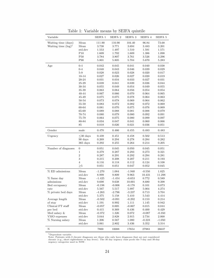
Table 1: Variable means by SEIFA quintile
Variable SEIFA 1 SEIFA 2 SEIFA 3 SEIFA 4 SEIFA 5
Waiting time (days) Mean 111.90 110.90 104.40 96.84 73.68Waiting time (log)† Mean 3.738 3.771 3.694 3.483 3.201
std.dev 1.553 1.497 1.510 1.591 1.571P10 1.609 1.792 1.609 1.386 1.098P50 3.784 3.807 3.761 3.526 3.296P90 5.801 5.805 5.704 5.670 5.283
Age 0-4 0.042 0.045 0.041 0.040 0.0380-4 0.048 0.043 0.046 0.039 0.0295-9 0.028 0.023 0.028 0.020 0.01710-14 0.027 0.026 0.027 0.020 0.01920-24 0.031 0.034 0.033 0.027 0.03125-29 0.039 0.041 0.039 0.036 0.04430-34 0.055 0.049 0.054 0.049 0.05535-39 0.063 0.064 0.056 0.054 0.05440-44 0.067 0.066 0.070 0.064 0.06545-49 0.075 0.075 0.078 0.064 0.06350-54 0.073 0.078 0.069 0.064 0.06255-59 0.083 0.072 0.082 0.072 0.06960-64 0.081 0.070 0.075 0.076 0.06965-69 0.089 0.088 0.081 0.088 0.07970-74 0.080 0.079 0.080 0.092 0.09175-79 0.064 0.075 0.080 0.099 0.09780-84 0.034 0.047 0.041 0.060 0.06685 0.018 0.026 0.021 0.036 0.051
Gender male 0.470 0.466 0.455 0.483 0.483
Urgency ≤30 days 0.439 0.451 0.458 0.502 0.51390 days 0.269 0.294 0.278 0.284 0.282365 days 0.292 0.255 0.264 0.214 0.205
Number of diagnoses 0 0.051 0.045 0.050 0.045 0.0511 0.279 0.287 0.293 0.273 0.3212 0.287 0.291 0.292 0.294 0.2813 0.215 0.208 0.207 0.211 0.1934 0.116 0.118 0.112 0.124 0.108≥5 0.051 0.051 0.047 0.052 0.045
% ED admissions Mean -1.270 1.084 -1.940 -0.550 1.825std.dev 8.999 9.809 9.963 10.431 11.298
% Same day Mean -1.425 -1.454 -0.653 0.772 0.589admissions std.dev 9.698 9.638 10.001 8.680 9.398Bed occupancy Mean -0.198 -0.006 -0.178 0.101 0.073rate std.dev 5.567 5.517 5.997 5.004 4.274% private bed days Mean -4.263 -2.796 -3.237 0.713 3.704
std.dev 5.375 5.158 5.410 5.543 4.414Average length Mean -0.502 -0.091 -0.292 0.153 0.214of stay std.dev 1.191 0.992 1.111 1.145 0.942Clinical FT staff Mean -0.057 0.005 -0.067 0.015 0.044per bed std.dev 0.415 0.369 0.436 0.400 0.429Med salary & Mean -0.372 1.326 0.072 -0.087 -0.350VMO expenses std.dev 3.044 2.828 2.915 2.734 2.068% Nursing salary Mean 1.206 0.567 1.080 -0.223 -1.050
std.dev 3.061 2.802 3.436 3.352 3.314
N 7800 10088 17654 27983 26637
†Dependent variable.Note: Patients with 0 chronic diagnoses are those who only have diagnoses that are not consideredchronic (e.g., short sightedness or hay fever). The 30 day urgency class pools the 7-day and 30-dayurgency categories used in NSW.
24

Table 2: Regression results (dependent variable: log waiting time)
Model 1 Model 2
Coeff t-stat Coeff t-stat
SEIFA 1 Least advantaged 20% 0.332 22.09 0.191 11.492 20% - 40% 0.352 26.01 0.237 15.883 40% - 60% 0.307 26.95 0.195 15.084 60% - 80% 0.192 19.14 0.160 15.31
Urgency 30 days or less -1.165 -122.88 -1.165 -123.26365 days (base: 90 days) 0.331 28.19 0.323 27.50
Age 0-4 -0.196 -6.64 -0.191 -5.735-9 -0.006 -0.21 -0.023 -0.7310-14 -0.064 -1.95 -0.083 -2.3515-19 -0.227 -7.03 -0.237 -7.1820-24 -0.184 -6.39 -0.185 -6.4325-29 -0.156 -6.07 -0.156 -6.1130-34 -0.133 -5.59 -0.131 -5.5335-39 -0.072 -3.14 -0.070 -3.0640-44 -0.008 -0.39 -0.008 -0.3650-54 0.023 1.11 0.022 1.0755-59 0.004 0.20 0.005 0.2360-64 0.002 0.08 0.000 0.0065-69 0.031 1.50 0.029 1.4270-74 0.049 2.43 0.048 2.3775-79 0.037 1.82 0.029 1.4280-84 0.063 2.78 0.048 2.1485 -0.018 -0.69 -0.030 -1.15
Number of 0 -0.327 -5.53 -0.333 -5.65diagnoses 2 0.019 0.34 0.022 0.40
3 0.012 0.11 0.014 0.134 0.008 0.05 0.007 0.04≥5 -0.001 0.00 -0.003 -0.01
Gender Male -0.014 -1.62 -0.015 -1.73
Supply % Admissions from emergency department 0.004 7.36% Same day admissions -0.004 -5.80Bed occupancy rate 0.021 17.75% private bed days -0.013 -11.48Average length of stay -0.090 -14.69Clinical FT staff per bed -0.096 -4.78% doctors & VMO payments 0.013 8.26% nurse salary -0.004 -1.64
Constant 3.348 56.98 3.434 58.39
R-sq 0.464 0.473
Note: also included in the model are 28 dummy variables for primary and up to five secondarydiagnoses (not mutually exclusive) and 196 dummy variables for procedures (the omitted groupis other surgical).
25

Tab
le3:
Dec
omp
osit
ion
ofov
eral
lpat
ient
and
supply
char
acte
rist
ics
SE
IFA
1S
EIF
A2
SE
IFA
3S
EIF
A4
10
50
90
10
50
90
10
50
90
10
50
90
vA−vB
0.5
110
0.4
884
0.5
174
0.6
930
0.5
108
0.5
220
0.5
108
0.4
654
0.4
206
0.2
877
0.2
306
0.3
867
v̂A−v̂B
0.5
055**
0.4
853**
0.5
146**
0.6
378**
0.5
052**
0.5
207**
0.5
489**
0.4
597**
0.4
200**
0.2
776**
0.2
321**
0.3
861**
Pati
ent
En
dow
men
t0.1
784**
0.1
693**
-0.0
307
0.2
108**
0.1
859**
-0.0
034
0.2
599**
0.2
018**
-0.1
208*
0.1
472**
0.1
031**
-0.0
087
Su
pp
lyE
nd
ow
men
t0.1
347**
0.1
249**
0.3
766**
0.0
125
0.0
879**
0.2
983**
0.1
939**
0.1
113**
0.3
426**
0.0
580*
0.0
628**
0.1
721**
Pati
ent
Tre
atm
ent
0.2
469**
0.0
6660
0.1
739*
0.2
717**
0.2
277**
0.2
670**
0.2
890**
0.1
603**
0.1
399**
0.1
807**
0.1
109**
0.2
127**
Su
pp
lyT
reatm
ent
-0.1
019
0.1
173*
-0.0
026
-0.0
268
-0.0
385
-0.0
666
-0.0
532
0.0
065
0.0
021
-0.0
074
0.0
000
0.0
357**
R̂1
-0.0
027
0.0
2180
0.1
131
-0.0
206
0.0
218
0.0
555
-0.1
785**
-0.0
305
0.1
541**
-0.0
872**
-0.0
473*
0.0
034
R̂2
0.0
501
-0.0
1470
-0.1
157
0.1
902*
0.0
204
-0.0
301
0.0
377
0.0
102
-0.0
979
-0.0
137
0.0
026
-0.0
291
Note
:st
ati
stic
al
sign
ifica
nce
isb
ase
don
boots
trap
ped
stan
dard
erro
rsw
ith
100
rep
lica
tion
s.*
an
d**
ind
icate
stati
stic
al
sign
ifica
nce
at
5%
an
d1%
resp
ecti
vel
y.B
ase
don
two-s
am
ple
mea
nd
iffer
ence
test
,ra
wgap
sare
all
stati
stic
ally
sign
ifica
nt
at
any
conven
tion
al
level
.
26

Tab
le4:
Det
aile
ddec
omp
osit
ion
ofsu
pply
char
acte
rist
ics
SE
IFA
1S
EIF
A2
SE
IFA
3S
EIF
A4
10
50
90
10
50
90
10
50
90
10
50
90
EN
DO
WM
EN
T
ED
0.0
444**
0.0
306**
0.0
480**
0.0
213**
0.0
147**
0.0
230**
0.0
670**
0.0
461**
0.0
724**
0.0
515**
0.0
355**
0.0
557**
Sam
ed
ay
-0.0
017
0.0
046
0.0
165*
-0.0
017
0.0
045
0.0
162*
-0.0
017
0.0
046
0.0
164*
0.0
002
-0.0
004
-0.0
015
Bed
-0.0
090
-0.0
165
-0.0
258
-0.0
045
-0.0
082
-0.0
129
-0.0
469**
-0.0
860**
-0.1
346**
-0.0
067*
-0.0
124**
-0.0
194**
Pri
vate
-0.1
285**
-0.0
369
0.1
893**
-0.1
005**
-0.0
288
0.1
480**
-0.1
483**
-0.0
425
0.2
184**
-0.0
722**
-0.0
207
0.1
063**
Com
ple
xit
y0.1
825**
0.0
941**
0.1
798**
0.1
029**
0.0
531**
0.1
014**
0.2
33**
0.1
202**
0.2
296**
0.0
515**
0.0
266**
0.0
508**
Sta
ff-0
.0069
0.0
102
0.0
362
-0.0
005
0.0
007
0.0
026
-0.0
154
0.0
229*
0.0
811**
-0.0
057
0.0
085*
0.0
301**
Doct
ors
&V
MO
0.0
039
-0.0
029
-0.0
064
-0.0
353**
0.0
263**
0.0
575**
0.0
269**
-0.0
201**
-0.0
439**
0.0
045*
-0.0
034*
-0.0
073*
Nu
rse
0.0
500
0.0
417*
-0.0
609
0.0
307
0.0
256
-0.0
374
0.0
792
0.0
661
-0.0
965
0.0
349
0.0
291*
-0.0
425
TR
EA
TM
EN
T
ED
0.0
109
0.0
024
0.0
073
0.0
101
-0.0
095
-0.0
064
-0.0
134
-0.0
062
-0.0
010
0.0
008
-0.0
004
0.0
032
Sam
ed
ay
0.0
244
0.0
243**
0.0
008
0.0
147
-0.0
043
-0.0
139
0.0
075
-0.0
002
0.0
055
-0.0
126*
-0.0
034
0.0
099*
Bed
-0.0
012
-0.0
006
0.0
112*
-0.0
001
0.0
000
0.0
003
-0.0
026
-0.0
019
0.0
086*
-0.0
004
-0.0
013
-0.0
002
Pri
vate
-0.0
795
0.1
772**
0.1
245
-0.0
095
-0.0
630*
-0.0
911*
-0.0
107
-0.0
024
0.0
561
-0.0
031
0.0
053
0.0
317**
Com
ple
xit
y-0
.1017
-0.0
200
-0.1
392**
-0.0
012
0.0
138*
-0.0
230**
-0.0
436
0.0
157
-0.0
835**
0.0
068
0.0
040
0.0
082
Sta
ff0.0
089
-0.0
095
-0.0
393
0.0
007
-0.0
008
0.0
006
0.0
329
0.0
239
-0.0
266
-0.0
018
-0.0
017
0.0
001
Doct
ors
&V
MO
-0.0
008
-0.0
099
-0.0
045
-0.0
309
0.0
091
0.0
172
-0.0
028
-0.0
004
0.0
004
0.0
015
0.0
001
0.0
003
Nu
rse
0.0
371
-0.0
465
0.0
366
-0.0
106
0.0
162
0.0
497*
-0.0
205
-0.0
221
0.0
426
0.0
015
-0.0
026
-0.0
175*
Note
:st
ati
stic
al
sign
ifica
nce
isb
ase
don
boots
trap
ped
stan
dard
erro
rsw
ith
100
rep
lica
tion
s.*
an
d**
ind
icate
stati
stic
al
sign
ifica
nce
at
5%
an
d1%
resp
ecti
vel
y.
27

Tab
le5:
Rob
ust
nes
sof
pat
ient
trea
tmen
teff
ect
SE
IFA
1S
EIF
A2
SE
IFA
3S
EIF
A4
Row
10
50
90
10
50
90
10
50
90
10
50
90
1O
rigin
al
sam
ple
0.2
469**
0.0
666
0.1
739*
0.2
717**
0.2
277**
0.2
670**
0.2
890**
0.1
603**
0.1
399**
0.1
807**
0.1
109**
0.2
127**
2C
ontr
ollin
gfo
rd
is-
tan
ce0.2
474**
0.0
893*
0.2
519**
0.3
054**
0.2
667**
0.3
710**
0.2
694**
0.1
495**
0.0
895
0.0
943**
0.1
229**
0.1
979**
3C
ontr
ollin
gfo
rP
HI
0.3
349*
0.1
416**
0.1
499*
0.2
121*
0.2
405**
0.2
299**
0.2
098**
0.1
595**
0.1
491**
0.1
783**
0.1
134**
0.1
984**
4R
estr
icte
dp
roce
du
res
0.2
464*
0.0
682
0.1
749*
0.3
174**
0.1
983**
0.3
267**
0.2
912**
0.1
249**
0.0
994**
0.1
020**
0.0
920**
0.2
261**
5H
om
ogen
ou
sin
com
e0.3
070**
0.1
038*
0.1
416*
0.2
796**
0.2
047**
0.2
799**
0.3
378**
0.1
508**
0.2
009**
0.1
417**
0.1
442**
0.2
263**
6N
on
-in
dig
enou
s,A
us-
tralian
born
,E
ngli
shm
ain
lan
gu
age
0.2
594**
0.0
930*
0.1
400
0.2
844**
0.2
199**
0.2
711**
0.3
245**
0.1
746**
0.1
515**
0.1
116**
0.1
467**
0.2
062**
7S
yd
ney
an
dre
gio
ns
wit
hm
ajo
rci
ties
0.3
051**
0.1
660**
0.3
151**
0.1
528**
0.1
491**
0.3
032**
0.1
937**
0.1
768**
0.3
418**
0.1
139**
0.0
858**
0.2
305**
Note
:st
ati
stic
al
sign
ifica
nce
isb
ase
don
boots
trap
ped
stan
dard
erro
rsw
ith
100
rep
lica
tion
s.*
an
d**
ind
icate
stati
stic
al
sign
ifica
nce
at
5%
an
d1%
resp
ecti
vel
y.
28

.1.2.3
kernel density
0.1
kernel density
02
46
8
ln(w
ait)
SE
IFA
1S
EIF
A 2
SE
IFA
3S
EIF
A 4
SE
IFA
5
Fig
ure
1:D
ensi
tyof
log
wai
ting
tim
es
29

0.1.2.3
kernel density
02
46
8ln
(wai
t)no
te: d
otte
d lin
e re
pres
ents
cou
nter
fact
ual d
istri
butio
n
SE
IFA
1 &
5
0.1.2.3
kernel density
02
46
8ln
(wai
t)no
te: d
otte
d lin
e re
pres
ents
cou
nter
fact
ual d
istri
butio
n
SE
IFA
2 &
5
0.1.2.3
kernel density
02
46
8ln
(wai
t)no
te: d
otte
d lin
e re
pres
ents
cou
nter
fact
ual d
istri
butio
n
SE
IFA
3 &
5
0.1.2.3
kernel density0
24
68
ln(w
ait)
note
: dot
ted
line
repr
esen
ts c
ount
erfa
ctua
l dis
tribu
tion
SE
IFA
4 &
5
Fig
ure
2:D
ensi
tyof
actu
alan
dco
unte
rfac
tual
log
wai
ting
tim
eby
SE
IFA
pai
r
30

-0.2
-0.10
0.1
0.2
0.3
0.4
0.5
10
20
30
40
50
60
70
80
90
SE
IFA
1
En
do
wm
en
t: P
ati
en
tE
nd
ow
me
nt:
Su
pp
ly
Tre
atm
en
t: P
ati
en
tT
rea
tme
nt:
Su
pp
ly
-0.2
-0.10
0.1
0.2
0.3
0.4
0.5
10
20
30
40
50
60
70
80
90
SE
IFA
2
En
do
wm
en
t: P
ati
en
tE
nd
ow
me
nt:
Su
pp
ly
Tre
atm
en
t: P
ati
en
tT
rea
tme
nt:
Su
pp
ly
-0.2
-0.10
0.1
0.2
0.3
0.4
0.5
10
20
30
40
50
60
70
80
90
SE
IFA
4
En
do
wm
en
t: P
ati
en
tE
nd
ow
me
nt:
Su
pp
ly
Tre
atm
en
t: P
ati
en
tT
rea
tme
nt:
Su
pp
ly
-0.2
-0.10
0.1
0.2
0.3
0.4
0.5
10
20
30
40
50
60
70
80
90
SE
IFA
3
En
do
wm
en
t: P
ati
en
tE
nd
ow
me
nt:
Su
pp
ly
Tre
atm
en
t: P
ati
en
tT
rea
tme
nt:
Su
pp
ly
Fig
ure
3:A
ggre
gate
endow
men
tan
dtr
eatm
ent
effec
ts
31

-0.012
-0.01
-0.008
-0.006
-0.004
-0.002
0
10 20 30 40 50 60 70 80 90
ED
-0.012
-0.01
-0.008
-0.006
-0.004
-0.002
0
0.002
10 20 30 40 50 60 70 80 90
Same day
0.02
0.04
0.06
0.08
0.1
0.12
Bed occupancy rates
-0.02
-0.01
0
0.01
0.02
10 20 30 40 50 60 70 80 90
Private bed days
0
10 20 30 40 50 60 70 80 90-0.03
-0.02
-0.3
-0.25
-0.2
-0.15
-0.1
-0.05
0
10 20 30 40 50 60 70 80 90
Complexity (length of stay)
-0.04
-0.02
0
0.02
0.04
0.06
10 20 30 40 50 60 70 80 90
Medical staff & VMO payments
-0.03
-0.02
-0.01
0
0.01
0.02
0.03
10 20 30 40 50 60 70 80 90
Nurse salary
-0.5
-0.4
-0.3
-0.2
-0.1
0
0.1
0.2
10 20 30 40 50 60 70 80 90
Clinical full-time staff
Figure 4: RIF regression coefficients for supply variables in SEIFA 5 samples
32

References
[1] Askildsen, J.E., Tor Helge, H. and Oddvar, K. (2010) Prioritization and patients’ rights:
Analysing the effect of a reform in the Norwegian hospital sector. Social Science and
Medicine 70(2), 199-208.
[2] Australian Bureau of Statistics. (2001) Census of Population and Housing: Socio-
Economic Indexes for Area’s (SEIFA). Technical Paper 2001 Cat 2039.0.55.001. ABS,
Canberra.
[3] Australian Institute of Health and Welfare. (2007) Australian Hospital Statistics 2005-
06. AIHW, Canberra.
[4] Blinder, A.S. (1973) Wage discrimination: Reduced form and structural estimates. Jour-
nal of Human Resources 8, 436 - 455.
[5] Blau, F.D. and Lawrence, M.K. (1992) The gender earnings gap: Learning from Inter-
national Comparisons. American Economic Review 82, 533-538.
[6] Cobb-Clark, D.A. and Hildebrand, V.A. (2006) The wealth of Mexican Americans.
Journal of Human Resources 41(4), 841-868.
[7] Commonwealth of Australia. (2009) A healthier future for all Australians: National
Health and Hospitals Reform Commission - Final report June 2009. Canberra.
[8] Curtis, A.J., Russell, C.O.H., Stoelwinder, J.U., et al. (2010) Waiting list and elective
surgery: Ordering the queue. Medical Journal of Australia 192(4), 217-220.
[9] Derrett, S. (2005) Booking Systems for Elective Services in New
Zealand, A report by the Centre for Health Planning and Man-
agement to the National Ethics Advisory Committee, New Zealand
(http://www.neac.health.govt.nz/moh.nsf/pagescm/519/$file/booking-systems-
elective-services-nz-feb05.pdf)
[10] Dimakou, S., Parkin, D., Devlin, N. and Appelby, J. (2009) Identifying the impact of
government targets on waiting times in the NHS. Health Care Management Science
12(1), 1-10.
33

[11] DiNardo, J., Fortin, N.M. and Lemieux, T. (1996) Labor market institutions and the dis-
tribution of wages, 1973-1992: A semiparametric approach. Econometrica 64(5), 1001-
1044
[12] Doiron, D.J. and Riddell, W.C. (1994) The impact of unionization on male-female
earnings differences in Canada. Journal of Human Resources 29, 504-534.
[13] Doyle, J.J. (2005) Health insurance, treatment, and outcomes: Using auto accidents as
health shocks. Review of Economics and Statistics 87(2), 256-270.
[14] Firpo, S., Fortin, N. and Lemieux, T. (2007) Decomposing wage dis-
tributions using recentered influence function regressions. Available:
http://www.economie.uqam.ca/pages/docs/Lemieux Thomas.pdf
[15] Firpo, S., Fortin, N. and Lemieux, T. (2009) Unconditional quantile regressions. Econo-
metrica 77(3), 953 - 973.
[16] Firpo, S., Fortin, N. and Lemieux, T. (2010) Decomposition methods in Economics.
NBER Working Paper 16045.
[17] Fiscella, K., Franks, P., Doescher M.P. and Saver B.G. (2002) Disparities in health care
by race, ethnicity, and language among the insured: findings from a national sample.
Medical Care 40(1), 52-59.
[18] Fortin, N. (2009) RIF-Regression STATA ado file from Firpo, Fortin and Lemieux
(2009). Downloadable: http://faculty.arts.ubc.ca/nfortin/datahead.html.
[19] Gravelle, H. and Siciliani, L. (2008) Is waiting time prioritisation welfare improving?
Health Economics 17, 167-184.
[20] Greengross, P., Grant, K. and Collini, E. (1999) The history and development of the UK
National Health Service 1948 1999. Health System Resource Centre, United Kingdom.
[21] Huynh, P.T., Schoen C., Osborn, R. and Holmgren, A.L. (2006) The US health care
divide: Disparities in primary care experiences by income. The Commonwealth Fund
Publication no. 900, New York.
[22] Hodge, W., Horsley, T., Albiani, D., et al. (2007) The consequences of waiting for
cataract surgery: A systematic review. Canadian Medical Association Journal 176(9),
1285-1290.
34

[23] Jann, B. (2008) The Blinder-Oaxaca decomposition for linear regression models. Stata
Journal 8(4), 453-479.
[24] Johar, M., Jones, G., Keane, M., Savage E. and Stavrunova, O. Forthcoming, Waiting
times for elective surgery and the decision to buy private health insurance, Health
Economics, DOI: 10.1002/hec.1707
[25] Johar, M. and Savage, E. (2010) Do private patients have shorter waiting times for
elective surgery? Evidence from New South Wales public hospitals. Economic Papers
29(2), 1-15.
[26] Leighton, K. L. and Flores G. (2005) Pay now or pay later: providing interpreter services
in health care. Health Affairs 24(2), 435-444.
[27] Lopez, L., Wilper, A.P., Cervantes, M., et al. (2010) Racial and sex differences in
emergency department triage assessment and test ordering for chest pain, 1997-2006.
Academic Emergency Medicine 17(8), 801-808.
[28] Lindsay, C.M. and Feigenbaum, B. (1984) Rationing by waiting lists. American Eco-
nomic Review 74(3), 404-417.
[29] MacCormick, A.D., Tan, C.P. and Parry, B.R. (2004) Priority assessment of patients
for elective general surgery: Game on? ANZ Journal of Surgery 74(3), 143-145.
[30] Noseworthy T.W., McGurran, J.J., Hadorn, D.C., et al. (2002) Waiting for scheduled
services in Canada: Development of priority-setting scoring systems. Journal of Evalu-
ation in Clinical Practice 9(1), 23-31.
[31] Oaxaca, R. (1973) Male-Female wage differentials in urban labor markets. International
Economic Review 14, 693 - 709.
[32] Oudhoff, J.P., Timmermans, D.R.M., Knol, D.L., et al. (2007) Waiting for elective
general surgery: Impact on health related quality of life and psychosocial consequences.
BMC Public Health 7, 164.
[33] Park, C.Y., Lee, M.A. and Epstein, A.J. (2009) Variation in emergency department
wait times for children by race/ethnicity and payment source. Health Services Research
44(6), 2022-2039.
35

[34] Pylypchuk, Y. and Selden, T.M. (2008) A discrete choice decomposition analysis of
racial and ethnic differences in children’s health insurance coverage. Journal of Health
Economics 27(4), 1109-1128.
[35] Private Health Insurance Administration Council. (2006) Operations of the Registered
Health Benefits Organisations Annual Report 2005-06. PHIAC, Canberra.
[36] Propper, C., Sutton, M., Whitnall, C. and Windmeijer, F. (2010) Incentives and targets
in hospital care: Evidence from a natural experiment. Journal of Public Economics 94,
318-335.
[37] Productivity Commission. (2008) Report on Government Services, Volume 2 Health,
Community Services and Housing. AGPS, Canberra.
[38] Savage E. and Wright D. (2003) Moral hazard and adverse selection in Australian private
hospitals: 1989-1990. Journal of Health Economics 22, 331-359.
[39] Siciliani, L. and Martin, S. (2007) An empirical analysis of the impact of choice on
waiting times. Health Economics 16, 763-779.
[40] Siciliani, L. and Verzulli, R. (2009) Waiting times and socioeconomic status among
elderly Europeans: Evidence from SHARE. Health Economics 18, 1295-1306.
[41] Siciliani, L. and Laudicella, M. (2010) Waiting time and socioeconomic status: Evidence
from England. HEDG working papers 2010/05.
[42] Wenzlow, A.T., Mullahy, J. and Wolfe, B. (2004) Understanding racial disparities in
health: The income-wealth paradox. La Follette School Working Paper 2004-008.
[43] Yoo HC., Gee GC. and Takeuchi D. (2009) Discrimination and health among Asian
American immigrants: disentangling racial from language discrimination. Social Science
and Medicine 68(4), 726-732.
36