Discretion Rather Than Rules? When Is Discretionary ... · over the timeless-perspective rule, this paper investigates the inﬂu-ence of structural and preference parameters on the

Discretion Rather Than Rules? When IsDiscretionary Policymaking Better Than the

Timeless Perspective?∗

Stephan SauerEuropean Central Bank

Discretionary monetary policy produces a dynamic loss inthe New Keynesian model in the presence of cost-push shocks.The possibility to commit to a specific policy rule can increasewelfare. A number of authors since Woodford (1999) haveargued in favor of a timeless-perspective rule as an optimalpolicy. The short-run costs associated with the timeless per-spective are neglected in general, however. Rigid prices, rela-tively impatient households, a high preference of policymakersfor output stabilization, and a deviation from the steady stateall worsen the performance of the timeless-perspective rule andcan make it inferior to discretion.

JEL Code: E5.

1. Introduction

Kydland and Prescott (1977) showed that rule-based policymakingcan increase welfare. The timeless perspective proposed by Wood-ford (1999) represents a prominent modern form of such a rule in

∗I would like to thank Julia Bersch, Frank Heinemann, Gerhard Illing, UliKluh, Bennett McCallum, Rudiger Pohl, Ludwig Rebner, the editor Carl Walsh,three anonymous referees, and seminar participants at the European CentralBank, the University of Munich, the IWH Halle, and the Xth Spring Meeting ofYoung Economists in Geneva for helpful comments, as well as Bennett McCallumand Christian Jensen for making their MATLAB code available to me. This paperis a revised chapter of my PhD thesis at the University of Munich, and part of itwas completed while I was visiting the Monetary Policy Strategy Division at theEuropean Central Bank; their hospitality is gratefully acknowledged. The viewsexpressed in this paper are my own and do not necessarily reflect those of theEuropean Central Bank or the Eurosystem. Author contact: Kaiserstr. 29, 60311Frankfurt am Main, Germany; E-mail: [email protected].

1

2 International Journal of Central Banking June 2010

monetary policy analysis. It helps to overcome not only the tradi-tional inflation bias in the sense of Barro and Gordon (1983a, 1983b)but also the stabilization bias, a dynamic loss stemming from cost-push shocks in the New Keynesian model as described in Clarida,Galı, and Gertler (1999). It is, however, associated with short-runcosts that may be larger than the long-run gains from commitment.

After deriving a formal condition for the superiority of discretionover the timeless-perspective rule, this paper investigates the influ-ence of structural and preference parameters on the performanceof monetary policy both under discretion and the timeless perspec-tive in the sense of Woodford (1999). Discretion gains relative to thetimeless-perspective rule—i.e., the short-run losses become relativelymore important—if the private sector behaves less forward lookingor if the monetary authority puts a greater weight on output-gapstabilization. For empirically reasonable values of price stickiness,the relative gain from discretion rises with stickier prices. A fourthparameter which influences the relative gains is the persistence ofshocks: Introducing serial correlation into the model only strength-ens the respective relative performance of policies in the situationwithout serial correlation in shocks. In particular, we show condi-tions for each parameter under which discretion performs strictlybetter than the timeless-perspective rule.

Furthermore, the framework of short-run losses and long-rungains also allows explaining why an economy that is sufficiently faraway from its steady state suffers rather than gains from imple-menting the timeless-perspective rule. In general, this paper usesunconditional expectations of the loss function as welfare criterion,in line with most of the literature. The analysis of initial condi-tions, however, requires reverting to expected losses conditional onthe initial state of the economy because unconditional expectationsof the loss function implicitly treat the economy’s initial conditionsas stochastic. Altogether, in the normal New Keynesian model, allconditions for the superiority of discretion need not be as adverse asone might suspect—in particular, if the initial output-gap situationis taken into account.

The following section 2 presents the canonical New Keynesianmodel. Section 3.1 explains the relevant welfare criteria. The ana-lytical solution in section 3.2 is followed by simulation results anda thorough economic interpretation of the performance of policies

Vol. 6 No. 2 Discretion Rather Than Rules? 3

under discretion and the timeless perspective. Section 3.4 completesthe discussion of Woodford’s timeless perspective by looking at theeffects of initial conditions before section 4 concludes.

2. New Keynesian Model

The New Keynesian or New Neoclassical Synthesis model hasbecome the standard toolbox for modern macroeconomics. Whilethere is some debate about the exact functional forms, the standardsetup consists of a forward-looking Phillips curve, an intertempo-ral IS curve, and a welfare function.1 Following, e.g., Walsh (2003),the New Keynesian Phillips curve based on Calvo (1983) pricing isgiven by

πt = βEtπt+1 + αyt + ut (1)

with

α ≡ (1 − ζ)(1 − βζ)ζ

. (2)

πt denotes inflation, Et the expectations operator conditional oninformation in period t, yt the output gap, and ut a stochastic shockterm that is assumed to follow a stationary AR(1) process withAR parameter ρ and innovation variance σ2. While the output gaprefers to the deviation of actual output from natural or flexible-priceoutput, ut is often interpreted as a cost-push shock term that cap-tures time-varying distortions from consumption or wage taxationor markups in firms’ prices or wages. It is the source of the stabiliza-tion bias. 0 < β < 1 denotes the (private sector’s) discount factorand 0 ≤ ζ < 1 is the constant probability that a firm is not able toreset its price in period t. A firm’s optimal price depends on currentand (for ζ > 0) future real marginal costs, which are assumed to beproportional to the respective output gap.2 Hence, ζ and α reflectthe degree of price rigidity in this model, which is increasing in ζand decreasing in α.

1Depending on the purpose of their paper, some authors directly use aninstrument rule or a targeting rule without explicitly maximizing some welfarefunction.

2In (1), the proportionality factor is set equal to 1.


The policymaker’s objective at an arbitrary time t = 0 is tominimize

L = E0

∞∑t=0

βtLt with Lt = π2t + ωy2

t , (3)

where ω ≥ 0 reflects the relative importance of output-gap variabil-ity in policymaker preferences. We assume zero to be the target valueof both inflation and the output gap. While the former assumptionis included only for notational simplicity and without loss of gener-ality, the latter is crucial for the absence of a traditional inflationbias in the sense of Barro and Gordon (1983a, 1983b).

The New Keynesian model also includes an aggregate demandrelationship based on consumers’ intertemporal optimization in theform of

yt = Etyt+1 − b(Rt − Etπt+1) + vt, (4)

where Rt is the central bank’s interest rate instrument and vt isa shock to preferences, government spending, or the exogenousnatural-rate value of output, for example.3 The parameter b > 0captures the output-gap elasticity with respect to the real interestrate. Yet, for distinguishing between the timeless-perspective anddiscretionary solutions, it is sufficient to assume that the centralbank can directly control πt as an instrument. Hence, the aggregatedemand relationship can be neglected below.4

2.1 Model Solutions

If the monetary authority neglects the impact of its policies on infla-tion expectations and reoptimizes in each period, it conducts mone-tary policy under discretion. This creates both the Barro and Gordon(1983a, 1983b) inflation bias for positive output-gap targets and theClarida, Galı, and Gertler (1999) stabilization bias caused by cost-push shocks. To concentrate on the second source of dynamic losses

3vt is generally referred to as a demand shock. But in this model, yt reflectsthe output gap and not output alone. Hence, shocks to the flexible-price level ofoutput are also included in vt. See, e.g., Woodford (2003, p. 246).

4Formally, adding (4) as a constraint to the optimization problems below givesa value of zero to the respective Lagrangian multiplier.


in this model, a positive inflation bias is ruled out by assuming anoutput-gap target of zero in the loss function (3). Minimizing (3)subject to (1) and to given inflation expectations Etπt+1 results inthe Lagrangian

Λt = π2t + ωy2

t − λt(πt − βEtπt+1 − αyt − ut) ∀ t = 0, 1, 2, . . . .(5)

The first-order conditions

∂Λt

∂yt= 2ωyt + αλt = 0

∂Λt

∂πt= 2πt − λt = 0

imply

πt = −ω

αyt. (6)

If instead the monetary authority takes the impact of its actionson expectations into account and possesses an exogenous possibil-ity to credibly commit itself to some future policy, it can minimizethe loss function (3) over an enhanced opportunity set. Hence, theresulting commitment solution must be at least as good as the oneunder discretion. The single-period Lagrangian (5) changes to

Λ = E0

∞∑t=0

βt[(

π2t + ωy2

t

)− λt(πt − βπt+1 − αyt − ut)

]. (7)

This yields as first-order conditions

∂Λ∂yt

= 2ωyt + αλt = 0, t = 0, 1, 2, . . . ,

∂Λ∂πt

= 2πt − λt = 0, t = 0,

∂Λ∂πt

= 2πt − λt + λt−1 = 0, t = 1, 2, . . . ,


implying

πt = −ω

αyt, t = 0 and (8)

πt = −ω

αyt +

ω

αyt−1, t = 1, 2, . . . . (9)

The commitment solution improves the short-run output/inflationtrade-off faced by the monetary authority because short-run pricedynamics depend on expectations about the future. Since theauthority commits to a history-dependent policy in the future, itis able to optimally spread the effects of shocks over several periods.The commitment solution also enables the policymaker to reap thebenefits of discretionary policy in the initial period without payingthe price in terms of higher inflation expectations, since these areassumed to depend on the future commitment to (9). Indeed, opti-mal policy is identical under commitment and discretion in the initialperiod. Nevertheless, the equilibrium outcomes for inflation and theoutput gap under the two policy regimes differ, as they also dependon inflation expectations and thus the prevailing policy regime. Ina recent paper, Dennis and Soderstrom (2006) compare the welfaregains from commitment over discretion under different scenarios.

However, the commitment solution suffers from time inconsis-tency in two ways: First, by switching from (9) to (6) in any futureperiod, the monetary authority can exploit given inflation expec-tations and gain in the respective period. Second, the monetaryauthority knows at t = 0 that applying the same optimization pro-cedure (7) in the future implies a departure from today’s optimalplan, a feature McCallum (2003, p. 4) calls “strategic incoherence.”

To overcome the second form of time inconsistency and thusgain true credibility, many authors since Woodford (1999) have pro-posed the concept of policymaking under the timeless perspective:The optimal policy in the initial period should be chosen such thatit would have been optimal to commit to this policy at a date farin the past, not exploiting given inflation expectations in the initialperiod.5 This implies neglecting (8) and applying (9) in all periods,not just in t = 1, 2, . . .:

5Woodford (1999) compares this “commitment” to the “contract” under JohnRawls’s veil of uncertainty. In a recent contribution, Loisel (2008) endogenizes


πt = −ω

αyt +

ω

αyt−1, t = 0, 1, . . . . (10)

Hence, the only difference to the commitment solution lies in thedifferent policy in the initial period, unless the economy starts fromits steady state with y−1 = 0.6 But since the commitment solutionis by definition optimal for (7), this difference causes a loss of thetimeless-perspective policy compared with the commitment solution.If this loss is greater than the gain from the commitment solution(COM) over discretion, rule-based policymaking under the timelessperspective (TP) causes larger losses than policy under discretion(DIS):

LTP − LCOM > LDIS − LCOM ⇔ LTP > LDIS . (11)

The central aim of the rest of this paper is to compare the lossesfrom TP and DIS.

2.2 Minimal State Variable (MSV) Solutions

Before we are able to calculate the losses under the different policyrules, we need to determine the particular equilibrium behavior ofthe economy, which is given by the New Keynesian Phillips curve(1)7 and the respective policy rule, i.e., DIS (6) or TP (10). FollowingMcCallum (1999), the minimal state variable (MSV) solution to eachmodel represents the rational-expectations solution that excludesbubbles and sunspots.

Under discretion, ut is the only relevant state variable in (1) and(6):

πt = βEtπt+1 + αyt + ut

πt = −ω

αyt,

the timeless perspective for certain calibrated parameter values following thereputation mechanism in Barro and Gordon (1983b).

6Due to the history dependence of (10), the different initial policy has someinfluence on the losses in subsequent periods, too.

7Without loss of generality but to simplify the notation, the MSV solutionsare derived based on (1) without reference to (2). The definition of α in (2) issubstituted into the MSV solutions for the simulation results in section 3.3.


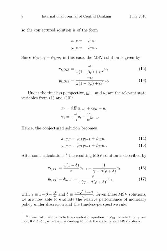
so the conjectured solution is of the form

πt,DIS = φ1ut

yt,DIS = φ2ut.

Since Etπt+1 = φ1ρut in this case, the MSV solution is given by

πt,DIS =ω

ω(1 − βρ) + α2 ut (12)

yt,DIS =−α

ω(1 − βρ) + α2 ut. (13)

Under the timeless perspective, yt−1 and ut are the relevant statevariables from (1) and (10):

πt = βEtπt+1 + αyt + ut

πt = −ω

αyt +

ω

αyt−1.

Hence, the conjectured solution becomes

πt,TP = φ11yt−1 + φ12ut (14)

yt,TP = φ21yt−1 + φ22ut. (15)

After some calculations,8 the resulting MSV solution is described by

πt,TP =ω(1 − δ)

αyt−1 +

1γ − β(ρ + δ)

ut (16)

yt,TP = δyt−1 − α

ω(γ − β(ρ + δ))ut, (17)

with γ ≡ 1+β + α2

ω and δ ≡ γ−√

γ2−4β

2β . Given these MSV solutions,we are now able to evaluate the relative performance of monetarypolicy under discretion and the timeless-perspective rule.

8These calculations include a quadratic equation in φ21, of which only oneroot, 0 < δ < 1, is relevant according to both the stability and MSV criteria.


3. Policy Evaluation

3.1 Welfare Criteria

3.1.1 Unconditional Expectations

The standard approach to evaluate monetary policy performance isto compare average values for the period loss function—i.e., valuesof the unconditional expectations of the period loss function in (3),denoted as E[Lt]. We follow this approach for the analysis of theinfluence of preference and structural parameters mainly because itis very common in the literature9 and allows an analytical solution.However, it includes several implicit assumptions.

First, πt and yt need to be covariance stationary. This is nota problem in our setup since ut is stationary by assumption and0 < δ < 1 is chosen according to the stability criterion; see foot-note 8. Second, using unconditional expectations of Lt implies treat-ing the initial conditions as stochastic (see, e.g., King and Wolman1999, p. 377) and thus averages over all possible initial conditions.Third, the standard approach treats all periods in the same wayas E[Lt] = E[Lt+j ] for all j ≥ 0. This may influence the preciseparameter values for which DIS performs better than TP in section3.3, but it only strengthens the general argument with respect tothe influence of β, as will be shown below.

3.1.2 Conditional Expectations

At the same time, using unconditional expectations impedes aninvestigation of the effects of specific initial conditions and tran-sitional dynamics to the steady state on the relative performance ofpolicy rules. For this reason and to be consistent with the micro-foundations of the New Keynesian model, Kim and Levin (2005),Kim et al. (2008), and Schmitt-Grohe and Uribe (2004) argue infavor of conditional expectations as the relevant welfare criterion. Iffuture outcomes are discounted—i.e., β < 1—the use of conditional

9See, e.g., various articles in the conference volume by Taylor (1999) andClarida, Galı, and Gertler (1999), Jensen and McCallum (2002), and Woodford(1999).


expectations—i.e., L in (3)—as welfare criterion implies that short-run losses from TP become relatively more important to the long-rungains compared with the evaluation with unconditional expectations.

Both concepts can be used to evaluate the performance of mone-tary policy under varying parameter values, and the results are quali-tatively equivalent. Besides its popularity and analytical tractability,the choice of unconditional expectations as the general welfare meas-ure has a third advantage: by implicitly averaging over all possibleinitial conditions and treating all periods the same, we can evalu-ate policies for all current and future periods and thus consider thepolicy problem from a “truly timeless” perspective in the sense ofJensen (2003), which does not bias our results in favor of discre-tionary policymaking. Only the analysis of the effects of differentinitial conditions requires reverting to conditional expectations.

3.2 Analytical Solution

In principle, the relative performance of DIS and TP can be solvedanalytically if closed-form solutions for the unconditional expec-tations of the period loss function are available. This is possible,since

Li = E[Lt,i] = E[π2

t,i

]+ ωE

[y2

t,i

], i ∈ {DIS ,TP} (18)

from (3) and the MSV solutions in section 2.2 determine the uncon-ditional variances E[π2

t,i] and E[y2t,i]. The MSV solution under

discretion, (12) and (13) with ut as the only state variable andE[u2

t ] = 11−ρ2 σ2, gives the relevant welfare criterion

LDIS =[

ω

ω(1 − βρ) + α2

]2 11 − ρ2 σ2

+ ω

[−α

ω(1 − βρ) + α2

]2 11 − ρ2 σ2

=ω(ω + α2)

[ω(1 − βρ) + α2]2· 11 − ρ2 σ2. (19)

For the timeless perspective, the MSV solution (16) and (17)depends on two state variables, yt−1 and ut. From the conjecturedsolution in (14) and (15), we have


E[π2

t,TP]

= φ211E

[y2

t−1]+ φ2

12E[u2

t

]+ 2φ11φ12E[yt−1ut]

E[y2

t,TP]

= φ221E

[y2

t−1]+ φ2

22E[u2

t

]+ 2φ21φ22E[yt−1ut]. (20)

These two equations are solved and plugged into (18) in the appen-dix. The result is

LTP =2ω(1 − δ)(1 − ρ) + α2(1 + δρ)

ω(1 − δ2)(1 − δρ)[γ − β(δ + ρ)]2· 11 − ρ2 σ2. (21)

Hence, discretion is superior to the timeless-perspective rule if

LDIS < LTP ⇔ ω(ω + α2)[ω(1 − βρ) + α2]2

<2ω(1 − δ)(1 − ρ) + α2(1 + δρ)

ω(1 − δ2)(1 − δρ)[γ − β(δ + ρ)]2

⇔ RL ≡ LTP/LDIS − 1 > 0. (22)

Equation (22) allows analytical proofs of several intuitive argu-ments: First, the variance of cost-push shocks 1

1−ρ2 σ2 affects themagnitude of absolute losses in (19) and (21) but has no effect on therelative loss RL because it cancels out in (22). Second, economic the-ory states that with perfectly flexible prices, i.e., ζ = 0 and α → ∞,the short-run Phillips curve is vertical at yt = 0. In this case, theshort-run output/inflation trade-off and hence the source of the sta-bilization bias disappears completely and no difference between DIS,COM, and TP can exist.

Third, if the society behaves as an “inflation nutter” (King 1997)and only cares about inflation stabilization—i.e., ω = 0—inflationdeviates from the target value neither under discretion nor underrule-based policymaking. This behavior eliminates the stabilizationbias because the effect of shocks cannot be spread over several peri-ods. Shocks always enter the contemporaneous output gap com-pletely, but they do not cause welfare losses for an inflation nutter.Furthermore, the initial conditions do not matter, since y−1 receivesa weight of 0 in (10) and no short-run loss arises. The last twostatements are summarized in the following proposition.

Proposition 1. Discretion and Woodford’s timeless perspective areequivalent for


(i) perfectly flexible prices or(ii) inflation-nutter preferences.

Proof.

(i) limα→∞ RL = 0.(ii) limω→0 RL = 0.

Finally, proposition 2 states that discretion is not always inferiorto Woodford’s timeless perspective. If the private sector discountsfuture developments at a larger rate—i.e., β decreases—firms careless about optimal prices in the future when they set their optimalprice today. Hence, the potential to use future policies to spread theeffects of a current shock via the expectations channel decreases.Therefore, the loss from the stabilization bias under DIS, where thispotential is not exploited (i.e., the long-run gains LDIS − LCOM ),also decreases with smaller β, while the short-run costs from TP,LTP − LCOM , remain unaffected under rule (10). In the extremecase of β = 0, expectations are irrelevant in the Phillips curve (1)and the source of the stabilization bias disappears. If the reductionin the long-run gain is sufficiently large, conditions (11) and (22) arefulfilled.

Proposition 2. There exists a discount factor β small enough suchthat discretion is superior to Woodford’s timeless perspective as longas some weight is given to output stabilization and prices are notperfectly flexible.

Proof. RL is continuous in β because stability requires 0 ≤ δ, ρ < 1.Furthermore, limβ→0 RL = [α2+2(1−ρ)ω+(1+ρ)ω](α2+ω)

(α2+2ω)[α2+(1−ρ)ω] − 1 > 0 forω > 0 ∧ α < ∞.

In principle, (22) could be used to look at the influence ofstructural (ζ, ρ) and preference (β, ω) parameters on the relativeperformance of monetary policy under discretion and the timeless-perspective rule more generally.10 Unfortunately, (22) is too complex

10Please note that, conceptually, it would be nonsense to compare one policyover several values of a preference parameter. Here, however, we always com-pare two policies (DIS and TP), holding all preference and structural parametersconstant.


Table 1. Parameter Values Used in the Benchmark Modeland Common in the Literature

Parameter β ω ζ α ρ

Benchmark Model 0.99 0.0625 0.8722 0.02 0Range in the Literature 0.97–1 0.01–0.25 0.73–0.91 0.01–0.1 0–0.95

to be analytically tractable. Hence, we have to turn to results fromsimulations.

3.3 Simulation Results

Preference (β, ω) and structural (ζ, ρ) parameters influence the rel-ative performance of monetary policy under discretion and thetimeless-perspective rule. To evaluate each effect separately, we startfrom a benchmark model with parameter values presented in table 1and then vary each parameter successively.

If one period in the model reflects one quarter, the discount fac-tor of β = 0.99 corresponds to an annual real interest rate of 4percent. Setting ω = 1/16 implies an equal weight on the quarterlyvariances of annualized inflation and the output gap. For β = 0.99,ζ = 0.8722 corresponds to α = 0.02, the value used in Jensen andMcCallum (2002) based on empirical estimates in Galı and Gertler(1999).11

To put the benchmark model into perspective, table 1 alsoreports the range of parameter values commonly used or estimated inthe literature. For example, Ljungqvist and Sargent (2004) calibratetheir model to β between 0.97 and 0.99.12 Furthermore, Rudebuschand Svensson (1999) justify the use of unconditional expectations astheir welfare criterion with the notion that conditional expectationsof the total loss function (3), scaled by (1 − β), and unconditionalexpectations of the period loss function, E[Lt], converge for β → 1

11ζ and α are linked through the definition of α in (2).12Note that Galı, Gertler, and Lopez-Salido (2001) estimate discount factors

in the Phillips curve as low as 0.91 for the euro area and 0.92 for the UnitedStates. The implied steady-state real interest rate of approximately 12 percentper annum for β = 0.97 is, however, substantially above the empirically observedrate of about 2 percent per annum in developed economies.


Figure 1. Variation of Discount Factor β, TP vs. DIS

(see also Dennis 2004). Hence, values between 0.97 and 1 are usedfor β in the literature, while β = 0.99 represents the most commonfigure. The ranges for ω (0.01 to 0.25), α (0.01 to 0.1), and thus via(2) also ζ (0.73 to 0.91) are taken from the discussion of the litera-ture in Walsh (2003, p. 527). Regarding the serial correlation of thecost-push shock, ρ, the literature covers a very broad range between0 and 0.95 (see, e.g., Kuester, Muller, and Stolting 2007). Figures1–5 in the remaining part of this section illustrate the parameterof the benchmark model as a dashed, vertical line and the range ofparameters in the literature as a gray-shaded area.

3.3.1 Discount Factor β

Figure 1 presents the results for the variation of the discount factor βas the loss from the timeless perspective relative to discretionary pol-icy, RL. A positive (negative) value of RL means that the loss fromthe timeless-perspective rule is greater (smaller) than the loss underdiscretion, while an increase (decrease) in RL implies a relative gain(loss) from discretion.

The simulation shows that RL increases with decreasing β; i.e.,DIS gains relative to TP if the private sector puts less weight on thefuture. This pattern reflects proposition 2 in the previous section.


Figure 2. Variation of Discount Factor β UsingConditional Expectations of Loss Function, TP vs. DIS

Since the expectations channel becomes less relevant with smaller β,the stabilization bias and thus the long-run gains from commitmentalso decrease in β, whereas short-run losses remain unaffected.

In particular, DIS becomes superior to TP in the benchmarkmodel for β < 0.839, but, e.g., with ω = 1 already for β < 0.975.13

Differentiating between the central bank’s and the private sector’sdiscount factor β (see McCallum 2005; Sauer 2007) shows that thelatter drives RL because it enters the Phillips curve, while the for-mer is irrelevant due to the use of unconditional expectations asthe welfare criterion, as discussed in section 3.1. But since using theunconditional expectations of the loss function treats all periods thesame and hence gives greater weight to future periods than actuallyvalid for β < 1, this effect only strengthens the general argument.

This can be shown with the value of the loss function (3),L = E0

∑∞t=0 βtLt, conditional on expectations at t = 0 instead

of the unconditional expectations E[L]. As figure 2 demonstrates,

13The threshold of β = 0.975 for ω = 1 is still a rather small value, as it impliesa steady-state real interest rate of approximately 10 percent per annum.


the general impact of β on RL is similar to figure 1.14 The notabledifference is the absolute superiority of DIS over TP in our bench-mark model, independently of β. In order to get a critical value of βfor which DIS and TP produce equal losses, other parameters of thebenchmark model have to be adjusted such that they favor TP, e.g.,by reducing ω as explained below. Hence, figure 2 provides evidencethat the use of unconditional expectations does not bias the resultstoward lower losses for discretionary policy. For reasons presented insection 3.1, we focus on unconditional expectations in this section.

3.3.2 Output-Gap Weight ω

In Barro and Gordon (1983b), the traditional inflation bias increasesin the weight on the output gap, while the optimal stabilizationpolicies are identical both under discretion and under commitment.In our intertemporal model without structural inefficiences, how-ever, the optimal stabilization policies are different under DIS andCOM/TP. The history dependence of TP in (10) improves the mon-etary authority’s short-run output/inflation trade-off in each periodbecause it makes today’s output gap enter tomorrow’s optimal pol-icy with the opposite sign, but with the same weight ω/α in bothperiods. Hence, optimal current inflation depends on the change inthe output gap under TP, but only on the contemporaneous outputgap under DIS. This way, rule-based policymaking eliminates thestabilization bias and reduces the relative variance of inflation andoutput gap, which is a prominent result in the literature.15

The short-run costs from TP arise because the monetary author-ity must be tough on inflation in the initial period. These short-runcosts increase with the weight on the output gap ω.16 The long-rungains from TP are caused by the size of the stabilization bias andthe importance of its elimination given by the preferences in the lossfunction. Equation (10) shows that increasing ω implies a softer pol-icy on inflation today but is followed by a tougher policy tomorrow.Although the effect of tomorrow’s policy is discounted by the privatesector with β, the size of the stabilization bias—i.e., the neglection of

14The use of conditional expectations requires setting the initial conditions—i.e., y−1 and u0—to specific values. In figure 2, y−1 = −0.02 and u0 = 0.

15See, e.g., Dennis and Soderstrom (2006) and Woodford (1999).16The optimal output gap yt under DIS is decreasing in ω; see equation (6).


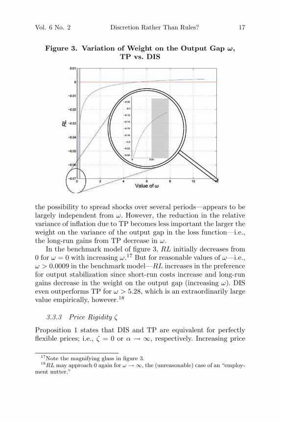
Figure 3. Variation of Weight on the Output Gap ω,TP vs. DIS

the possibility to spread shocks over several periods—appears to belargely independent from ω. However, the reduction in the relativevariance of inflation due to TP becomes less important the larger theweight on the variance of the output gap in the loss function—i.e.,the long-run gains from TP decrease in ω.

In the benchmark model of figure 3, RL initially decreases from0 for ω = 0 with increasing ω.17 But for reasonable values of ω—i.e.,ω > 0.0009 in the benchmark model—RL increases in the preferencefor output stabilization since short-run costs increase and long-rungains decrease in the weight on the output gap (increasing ω). DISeven outperforms TP for ω > 5.28, which is an extraordinarily largevalue empirically, however.18

3.3.3 Price Rigidity ζ

Proposition 1 states that DIS and TP are equivalent for perfectlyflexible prices; i.e., ζ = 0 or α → ∞, respectively. Increasing price

17Note the magnifying glass in figure 3.18RL may approach 0 again for ω → ∞, the (unreasonable) case of an “employ-

ment nutter.”


Figure 4. Variation of Degree of Price Rigidity ζ,TP vs. DIS

rigidity—i.e., increasing ζ—has two effects: First, firms’ price settingbecomes more forward looking because they have fewer opportunitiesto adjust their prices. This effect favors TP over DIS for increasing ζbecause TP optimally incorporates forward-looking expectations.Second, more rigid prices imply a flatter Phillips curve, and thusthe requirement of TP to be tough on inflation already in the initialperiod becomes more costly. Hence, the left-hand side of (11), theshort-run losses from TP over DIS, increases. Figure 4 demonstratesthat for ζ > 0.660, the second effect becomes more important andfor ζ > 0.959, the second effect even dominates the first one.19

Based on the discussion of the literature in Walsh (2003), com-mon estimates for price rigidity lie within α ∈ [0.01; 0.10]; i.e.,ζ ∈ [0.909; 0.733]. In this range, figure 4 shows that RL increaseswith the firms’ probability of not being able to reset their price, ζ,and exceeds 0 for ζ > 0.959 or α < 0.002.

19Since the relationship between ζ and α given by equation (2) also dependson β, there is a qualitatively irrelevant and quantitatively negligible differencebetween varying the probability of no change in a firm’s price, ζ, and directlyvarying the output-gap coefficient in the Phillips curve, α.


Figure 5. Variation of Degree of Serial Correlation ρ,TP vs. DIS

3.3.4 Correlation of Shocks ρ

The analysis of the influence of serial correlation in cost-push shocks,ρ, is more complex. LDIS exceeds LTP in the benchmark model withρ = 0, and raising ρ ceteris paribus strengthens the advantage of TPas demonstrated in the solid line in figure 5. If shocks become morepersistent, their impact on future outcomes increases, and thus TPgains relative to DIS because it accounts for these effects in a supe-rior way. The long-run gains from TP dominate its short-run losses,and RL decreases with ρ.

However, the relationship between ρ and RL is not independentof the other parameters in the model, while the relationships betweenRL and β, ζ, and ω, respectively, appear to be robust to alterna-tive specifications of other parameters. Broadly speaking, as long asLDIS > LTP for ρ = 0, varying ρ results in a diagram similar tothe solid line in figure 5; i.e., LDIS > LTP for all ρ ∈ [0; 1), and RLdecreases in ρ.

On the contrary, an appropriate combination of β, ζ, and ω canlead to LDIS ≤ LTP for ρ = 0. For example, the combination ofa low discount factor with rigid prices and a high preference foroutput-gap stabilization—such as the values β = 0.97, ζ = 0.91, andω = 0.25 reported from the literature in table 1—results in RL > 0.


In this case, a picture symmetric to the horizontal axis emerges, asshown by the dashed line in figure 5.20 That means that a higherdegree of serial correlation only strengthens the dominance of eitherTP or DIS already present without serial correlation. Hence, serialcorrelation on its own does not seem to be able to overcome theresult of the trade-off between short-run losses and long-run gainsfrom TP implied by the other parameter values.21

3.4 Effects of Initial Conditions

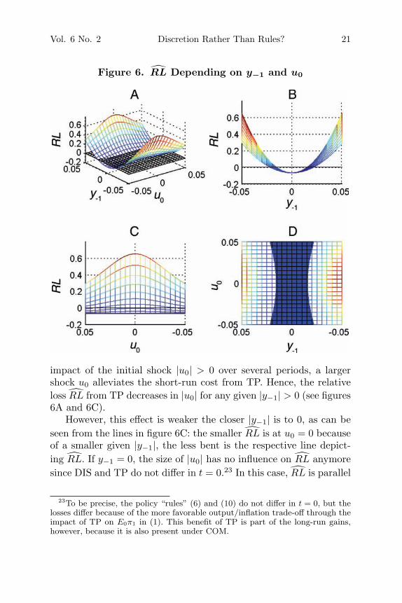
As argued in section 3.1, we have to use conditional expectations ofL in (3) in order to investigate the effects of the initial conditions—i.e., the previous output gap y−1 and the current cost-push shocku0—on the relative performance of policy rules. Figure 6 presentsthe relative loss RL = LTP/LDIS − 1 conditional on y−1 and u0 inthe range between –0.05 and 0.05 from different viewpoints.22

Starting from the steady state with y−1 = u0 = 0 whereRL = −0.0666 in the benchmark model, increasing the absolutevalue of the initial lagged output gap |y−1| increases the short-runcost from following TP instead of DIS and leaves long-run gainsunaffected: While π0,DIS = y0,DIS = 0 from (12) and (13), π0,TP andy0,TP deviate from their target values as can be seen from the historydependence of (10) or the MSV solution (16) and (17). Hence, TPbecomes suboptimal under conditional expectations for sufficientlylarge |y−1|. Note also that this short-run cost is symmetric to thesteady-state value y−1 = 0 (see figures 6A and 6B).

If in addition to |y−1| > 0 a cost-push shock |u0| > 0 hits theeconomy, the absolute losses under both DIS and TP increase. SinceTP allows an optimal combination of the short-run cost from TP,the inclusion of |y−1| > 0 in (10), with the possibility to spread the

20For parameter combinations that result in LDIS in the neighborhood of LTPfor ρ = 0, increasing ρ has hardly any influence on RL, but for high degrees ofserial correlation from about ρ > 0.8, RL increases rapidly.

21This shows that the results in McCallum and Nelson (2004, p. 48), whoonly report the relationship visible from the solid line in figure 5, do not hold ingeneral.

22Figure 6A offers the complete three-dimensional perspective of RL with anadditional plane marking RL = 0; figure 6B turns to the y−1 − RL perspectiveand figure 6C to the u0 − RL perspective; figure 6D provides the birds-eye view,with the shaded area signaling RL < 0.


Figure 6. RL Depending on y−1 and u0

impact of the initial shock |u0| > 0 over several periods, a largershock u0 alleviates the short-run cost from TP. Hence, the relativeloss RL from TP decreases in |u0| for any given |y−1| > 0 (see figures6A and 6C).

However, this effect is weaker the closer |y−1| is to 0, as can beseen from the lines in figure 6C: the smaller RL is at u0 = 0 becauseof a smaller given |y−1|, the less bent is the respective line depict-ing RL. If y−1 = 0, the size of |u0| has no influence on RL anymoresince DIS and TP do not differ in t = 0.23 In this case, RL is parallel

23To be precise, the policy “rules” (6) and (10) do not differ in t = 0, but thelosses differ because of the more favorable output/inflation trade-off through theimpact of TP on E0π1 in (1). This benefit of TP is part of the long-run gains,however, because it is also present under COM.


to the u0-axis. While u0 still influences the absolute loss values Lunder both policies and how these losses are spread over time underTP, it has no influence on the relative gain from TP as measured byRL, which is solely determined by the long-run gains from TP fory−1 = 0.

The shaded area in figure 6D summarizes the previous infor-mation, as it illustrates all combinations of u0 and y−1 for whichRL < 0. DIS is superior to TP for all other combinations of u0 andy−1.

Note that RL is symmetric both to y−1 = 0 for any given u0 andto u0 = 0 for any given y−1. Under DIS, y−1 has no impact because(6) is not history dependent and u0 only influences the respectiveperiod loss L0, which is the weighted sum of the variances π2

0 andy20. Hence, LDIS is independent of y−1 and symmetric to u0 = 0.

Under TP, however, the history dependence of (9) makes y−1 andu0 influence current and future losses. While the transitional dynam-ics differ with the relative sign of u0 and y−1, the total absoluteloss LTP does not for any given combination of |y−1| and |u0|. Ifthe economy was in a recession (y−1 < 0) in the previous period,for example,24 the price to pay under TP is to decrease π0 throughdampening y0 with a ceteris paribus restrictive monetary policy thatlowers aggregate demand.

Scenario 1. If additionally a negative cost-push shock u0 < 0hits the economy—i.e., with the same sign as y−1 < 0—this shocklowers π0 further as the Phillips curve (1) is shifted downward fromits steady-state locus. At the same time, u0 < 0 increases y0 ceterisparibus,25 brings y0 closer to the target of 0, and thus reduces theprice to pay for TP in the next periods t = 1, . . .. The anticipationof this policy in turn lowers inflation expectations E0π1 comparedwith the steady state. Therefore, the Phillips curve shifts even fur-ther down and the output gap y0 closes even more in the resultingequilibrium.

24The following arguments run in a completely analogous manner for y−1 > 0(see Sauer 2010).

25Formally, partial derivatives of (16) and (17) with respect to both state vari-ables (yt−1, ut) show that both have the same qualitative effect on πt and anopposing effect on yt: ∂πt/∂yt−1 = ω(1−δ)

α> 0 and ∂πt/∂ut = 1

γ−β(ρ+δ) > 0while ∂yt/∂yt−1 = δ > 0 and ∂yt/∂ut = −α

ω(γ−β(ρ+δ)) < 0.


Figure 7. Discounted Per-Period Loss Values LTP,t for|y−1| and |u0|

Scenario 2. If, however, the initial cost-push shock u0 ispositive—i.e., of opposite sign to y−1 < 0—the transitional dynamicsare reversed. The Phillips curve (1) is shifted upward. In contrast toscenario 1 with u0 < 0, this reduces the negative impact of y−1 on π0but increases y0. Hence, the price to pay under TP in t = 1 is largerthan in scenario 1, which in turn also lowers inflation expectationsE0π1 by more. The additional shift of the Phillips curve downwardis thus larger than for u0 < 0.

Figure 7 presents the discounted period losses under TP for bothcases in the benchmark model. The behavior of the economy asdescribed above causes a larger loss in the initial period for thefirst scenario with sign(y−1) = sign(u0) compared with the casewith sign(y−1) = −sign(u0) because the expectations channel has asmaller impact; but it causes a reversal of the magnitude of lossesfor t ≥ 1 because the price to pay for TP then is larger until theperiod loss converges to its unconditional value. Since the sum ofthe discounted losses, however, is equal in both scenarios, LTP issymmetric to u0 = 0 given y−1 and to y−1 = 0 given u0.

To summarize, figure 6 presents the influences of the initial con-ditions on the relative performance of TP and DIS and the rest


of this section provides intuitive explanations of the effects presentin the model. RL becomes positive—i.e., DIS performs better thanTP—in the benchmark model for quite realistic values of the initialconditions, e.g., RL > 0 for |y−1| = 0.015 and |u0| = 0.01. Hence,it may not be welfare increasing for an economy to switch from DISto TP if it is not close to its steady state.

The previous sections 3.2 and 3.3 demonstrated, based on uncon-ditional expectations as welfare criterion, the possibility that DISoutperforms TP for some rather extreme combinations of parame-ters. This section has highlighted three points: First, the use ofconditional expectations as a welfare criterion may have importantconsequences for the evaluation of different policies (see also Kim etal. 2008; Schmitt-Grohe and Uribe 2004, for example). Second, therelevance of the results presented in this paper may be non-negligiblein practice given that already small deviations from the steadystate suffice to make discretion superior to the timeless-perspectiverule. Third, other papers have shown that a timeless-perspectiverule exists that is optimal for all combinations of parameters underunconditional expectations as welfare criterion (Blake 2001; Dam-janovic, Damjanovic, and Nolan 2008; Jensen and McCallum 2002;Sauer 2007). However, this rule results in a diagram that is simi-lar to figure 6 when its performance is evaluated for different initialconditions under conditional expectations (see Sauer 2007). For anytimeless rule, initial conditions and hence the short-run costs can besufficiently adverse to make the rule inferior to discretion.

4. Conclusion

This paper explores the theoretical implications of the timeless-perspective policy rule and discretionary policy under varyingparameters in the New Keynesian model. With the comparison ofshort-run gains from discretion over rule-based policy and long-runlosses from discretion, we have provided a framework in which tothink about the impact of different parameters on monetary policyrules versus discretion. This framework allows intuitive economicexplanations of the effects at work.

Already Blake (2001), Jensen (2003), and Jensen and McCallum(2002) provide evidence that a policy rule following the timeless


perspective can cause larger losses than purely discretionary modesof monetary policymaking in special circumstances. But none ofthese contributions considers an economic explanation for this ratherunfamiliar result, let alone analyzes the relevant parameters as rig-orously as this paper.

What recommendations for economic policymaking can bederived? Most importantly, the timeless perspective in its standardformulation is not optimal for all economies at all times. Consider-ing each parameter separately, the critical values obtained in thispaper require a lower discount factor, a greater degree of price rigid-ity, or a higher preference for output stabilization than calibratedor estimated in most of the literature. But if an economy features acombination of these characteristics and in particular a sufficientlylarge deviation from its steady state, the long-run losses from dis-cretion may be less relevant than previously thought. In this case,discretionary monetary policy appears preferable over the timelessperspective.

In an overall laudatory review of Woodford (2003), Walsh (2005)argues that Woodford’s book “will be widely recognized as the defini-tive treatise on the new Keynesian approach to monetary policy.” Hecriticizes the book, however, for its lack of an analysis of the poten-tial short-run costs of adopting the timeless-perspective rule. Walsh(2005) sees these short-run costs arising from incomplete credibilityof the central bank. Our analysis has completely abstracted fromsuch credibility effects and still found potentially significant short-run costs from the timeless perspective. Obviously, if the privatesector does not fully believe in the monetary authority’s commit-ment, the losses from sticking to a rule relative to discretionarypolicy are even greater than in the model used in this paper. Oneway to incorporate such issues is to assume that the private sec-tor has to learn the monetary policy rule. Evans and Honkapohja(2001) provide a convenient framework to analyze this question inmore detail.

Appendix. Derivation of LTP

The unconditional loss for the timeless perspective, equation (21),can be derived in several steps. The MSV solution (16) and (17)


depends on two state variables, yt−1 and ut. From the conjecturedsolution in (15), we have

E[y2

t

]= φ2

21E[y2

t−1]+ φ2

22E[u2

t

]+ 2φ21φ22E[yt−1ut]. (23)

E[yt−1ut] can be calculated from (15) with ut = ρut−1 + ε as

E[yt−1ut] = E[(φ21yt−2 + φ22(ρut−2 + εt−1))(ρut−1 + εt)]

= E

⎡⎢⎣φ21ρ yt−2ut−1︸︷︷︸

=E[yt−1ut]

+φ22

⎛⎜⎝ρ2 ut−1ut−2︸︷︷︸

=ρσ2u

+ρ ut−1εt−1︸︷︷︸=σ2

⎞⎟⎠

⎤⎥⎦ + 3 · 0,

(24)

since the white-noise shock εt is uncorrelated with anything fromthe past. Solving for E[yt−1ut] with σ2

u = 11−ρ2 σ2 gives

E[yt−1ut] =φ22ρ

1 − φ21ρ· 11 − ρ2 σ2. (25)

Plugging this into (23), using E[y2t ] = E[y2

t−1] = E[y2] andφ21, φ22 from the MSV solution (17) leaves

E[y2] =1

1 − φ221

(φ2

22 +2φ21φ

222ρ

1 − φ21ρ

)1

1 − ρ2 σ2

=α2(1 + δρ)

ω2(1 − δ2)(1 − δρ)[γ − β(δ + ρ)]2· 11 − ρ2 σ2. (26)

From the conjectured solution in (14), we have

E[π2

t

]= φ2

11E[y2

t−1]+ φ2

12E[u2

t

]+ 2φ11φ12E[yt−1ut]. (27)

Combining this with the previous results and the MSV solution (16)results in

E[π2] =2(1 − ρ)

(1 + δ)(1 − δρ)[γ − β(δ + ρ)]2· 11 − ρ2 σ2. (28)

Hence, LTP as the weighted sum of E[π2] and E[y2] is given by

LTP =2ω(1 − δ)(1 − ρ) + α2(1 + δρ)

ω(1 − δ2)(1 − δρ)[γ − β(δ + ρ)]2· 11 − ρ2 σ2. (29)


References

Barro, R. J., and D. B. Gordon. 1983a. “A Positive Theory ofMonetary Policy in a Natural-Rate Model.” Journal of PoliticalEconomy 91 (4): 589–610.

———. 1983b. “Rules, Discretion and Reputation in a Model ofMonetary Policy.” Journal of Monetary Economics 12 (1): 101–21.

Blake, A. P. 2001. “A ‘Timeless Perspective’ on Optimalityin Forward-Looking Rational Expectations Models.” WorkingPaper, National Institute of Economic and Social Research.

Calvo, G. A. 1983. “Staggered Prices in a Utility-Maximizing Frame-work.” Journal of Monetary Economics 12 (3): 383–98.

Clarida, R., J. Galı, and M. Gertler. 1999. “The Science of Mone-tary Policy: A New Keynesian Perspective.” Journal of EconomicLiterature 37 (4): 1661–1707.

Damjanovic, T., V. Damjanovic, and C. Nolan. 2008. “Uncondition-ally Optimal Monetary Policy.” Journal of Monetary Economics55 (3): 491–500.

Dennis, R. 2004. “Solving for Optimal Simple Rules in RationalExpectations Models.” Journal of Economic Dynamics & Con-trol 28 (8): 1635–60.

Dennis, R., and U. Soderstrom. 2006. “How Important Is Precom-mitment for Monetary Policy?” Journal of Money, Credit, andBanking 38 (4): 847–72.

Evans, G. W., and S. Honkapohja. 2001. Learning and Expectationsin Macroeconomics. Princeton, NJ: Princeton University Press.

Galı, J., and M. Gertler. 1999. “Inflation Dynamics: A StructuralEconometric Analysis.” Journal of Monetary Economics 44 (2):195–222.

Galı, J., M. Gertler, and J. D. Lopez-Salido. 2001. “European Infla-tion Dynamics.” European Economic Review 45 (7): 1237–70.

Jensen, C. 2003. “Improving on Time-Consistent Policy: The Time-less Perspective and Implementation Delays.” Working Paper,GSIA, Carnegie Mellon University.

Jensen, C., and B. T. McCallum. 2002. “The Non-optimality of Pro-posed Monetary Policy Rules under Timeless-Perspective Com-mitment.” Economics Letters 77 (2): 163–68.


Kim, J., S. Kim, E. Schaumburg, and C. A. Sims. 2008. “Calculat-ing and Using Second-Order Accurate Solutions of Discrete TimeDynamic Equilibrium Models.” Journal of Economic Dynamics& Control 32 (11): 3397–3414.

Kim, J., and A. Levin. 2005. “Conditional Welfare Comparisons ofMonetary Policy Rules.” Mimeo (March).

King, M. 1997. “Changes in U.K. Monetary Policy: Rules and Dis-cretion in Practice.” Journal of Monetary Economics 39 (1):81–97.

King, R. G., and A. L. Wolman. 1999. “What Should the Mone-tary Authority Do When Prices Are Sticky?” In Monetary PolicyRules, ed. J. B. Taylor, 349–98. Chicago: University of ChicagoPress.

Kuester, K., G. J. Muller, and S. Stolting. 2007. “Is the New Key-nesian Phillips Curve Flat?” ECB Working Paper No. 809.

Kydland, F. E., and E. C. Prescott. 1977. “Rules Rather than Discre-tion: The Inconsistency of Optimal Plans.” Journal of PoliticalEconomy 85 (3): 473–91.

Ljungqvist, L., and T. J. Sargent. 2004. “European Unemploymentand Turbulence Revisited in a Matching Model.” Journal of theEuropean Economic Association 2 (2–3): 456–68.

Loisel, O. 2008. “Central Bank Reputation in a Forward-LookingModel.” Journal of Economic Dynamics & Control 32 (11):3718–42.

McCallum, B. T. 1999. “Role of the Minimal State Variable Cri-terion in Rational Expectations Models.” International Tax andPublic Finance 6 (4): 621–39.

———. 2003. “Comment on Athey, Atkeson, and Kehoe, ‘The Opti-mal Degree of Monetary Policy Discretion’.” Second Interna-tional Research Forum on Monetary Policy, Washington, DC,November 14–15.

———. 2005. “What Is the Proper Perspective for Monetary PolicyOptimality?” Monetary and Economic Studies (Bank of Japan)23 (S1): 13–24.

McCallum, B. T., and E. Nelson. 2004. “Timeless Perspective vs.Discretionary Monetary Policy in Forward-Looking Models.”Review (Federal Reserve Bank of St. Louis) 86 (2): 43–56.

Rudebusch, G. D., and L. E. O. Svensson. 1999. “Policy Rules forInflation Targeting.” In Monetary Policy Rules, ed. J. B. Taylor,203–46. Chicago: University of Chicago Press.


Sauer, S. 2007. Frameworks for the Theoretical and Empirical Analy-sis of Monetary Policy. PhD thesis, University of Munich. Avail-able at http://edoc.ub.uni-muenchen.de/7179/.

———. 2010. “When Discretion Is Better: Initial Conditions andthe Timeless Perspective.” Forthcoming in Economics Letters.

Schmitt-Grohe, S., and M. Uribe. 2004. “Optimal OperationalMonetary Policy in the Christiano-Eichenbaum-Evans Modelof the U.S. Business Cycle.” Working Paper. Available athttp://www.econ.duke.edu/∼grohe/research/index.html.

Taylor, J. B. 1999. Monetary Policy Rules. Chicago: University ofChicago Press.

Walsh, C. E. 2003. Monetary Theory and Policy. 2nd ed. Cambridge,MA: MIT Press.

———. 2005. “Interest and Prices: A Review Essay.” MacroeconomicDynamics 9 (3): 462–68.

Woodford, M. 1999. “Commentary: How Should Monetary PolicyBe Conducted in an Era of Price Stability?” In New Challengesfor Monetary Policy, 277–316. Federal Reserve Bank of KansasCity.

———. 2003. Interest and Prices: Foundations of a Theory of Mon-etary Policy. Princeton, NJ: Princeton University Press.

Documents

Discretion Rather Than Rules? When Is Discretionary ... · over the timeless-perspective rule, this paper investigates the inﬂu-ence of structural and preference parameters on the