Discretelinecomplexesand …rspa.royalsocietypublishing.org/content/royprsa/471/2175/...to be guaranteed by Desargues’ classical theorem of projective geometry. A remarkable characterization

rspa.royalsocietypublishing.org

ResearchCite this article: Bobenko AI, Schief WK. 2015Discrete line complexes and integrableevolution of minors. Proc. R. Soc. A 471:20140819.http://dx.doi.org/10.1098/rspa.2014.0819

Received: 20 October 2014Accepted: 14 January 2015

Subject Areas:geometry, mathematical physics

Keywords:line complex, discrete integrable system,Desargues’ theorem, correlation, projectivegeometry

Author for correspondence:W. K. Schiefe-mail: [email protected]

Discrete line complexes andintegrable evolution of minorsA. I. Bobenko1 and W. K. Schief2,3

1Institut für Mathematik, Technische Universität Berlin, Straße des17. Juni 136, 10623 Berlin, Germany2School of Mathematics and Statistics and 3Australian ResearchCouncil Centre of Excellence for Mathematics and Statistics ofComplex Systems, The University of New South Wales, Sydney,New South Wales 2052, Australia

Based on the classical Plücker correspondence, wepresent algebraic and geometric properties of discreteintegrable line complexes in CP

3. Algebraically, theseare encoded in a discrete integrable system thatappears in various guises in the theory of continuousand discrete integrable systems. Geometrically, theexistence of these integrable line complexes is shownto be guaranteed by Desargues’ classical theorem ofprojective geometry. A remarkable characterization interms of correlations of CP

3 is also recorded.

1. IntroductionLine congruences, that is, two-parameter families of lines,constitute fundamental objects in classical differentialgeometry [1]. In particular, normal and Weingartencongruences have been studied in great detail [2].Their importance in connection with the geometrictheory of integrable systems has been well documented(see [3] and references therein). Recently, in thecontext of integrable discrete differential geometry [4],attention has been drawn to discrete line congruences [5],that is, two-parameter families of lines which are(combinatorially) attached to the vertices of a Z

2 lattice.Discrete Weingarten congruences have been shown tolie at the heart of the Bäcklund transformation fordiscrete pseudo-spherical surfaces [6–8]. Discrete normalcongruences have been used to define Gaussian andmean curvatures and the associated Steiner formula fordiscrete analogues of surfaces parametrized in terms ofcurvature coordinates [9–11]. Discrete line congruenceshave also found important applications in architecturalgeometry [12].

2015 The Author(s) Published by the Royal Society. All rights reserved.

on June 28, 2018http://rspa.royalsocietypublishing.org/Downloaded from

http://crossmark.crossref.org/dialog/?doi=10.1098/rspa.2014.0819&domain=pdf&date_stamp=2015-02-11

mailto:[email protected]

http://rspa.royalsocietypublishing.org/

2

rspa.royalsocietypublishing.orgProc.R.Soc.A471:20140819

...................................................

Here, we are concerned with the extension of discrete line congruences in a three-dimensionalcomplex projective space CP

3 to three-dimensional ‘lattices of lines’, that is, maps of the form

l : Z3 → {lines in CP

3}. (1.1)

The latter define three-parameter families of lines which may be termed discrete line complexes.In the following, attention could be restricted to discrete line complexes in a real projectivespace RP

3. However, in order to analyse integrable line complexes in classical (Lie and Plücker)subgeometries of projective geometry, it is required to consider a complex ambient space. Thecorresponding rich geometric structure is the subject of a forthcoming publication. Discrete linecomplexes in a four-dimensional (projective) space have been shown to be integrable if anytwo neighbouring lines intersect [5]. Here, integrability is understood in the sense of multi-dimensional consistency, that is, in a well-defined sense, these discrete line complexes may beextended to Z

N lattices of lines such that the restriction to any Z3 sublattice constitutes a discrete

line complex.This paper is based on the observation that a system of algebraic equations which arises

in various avatars in the theory of both continuous and discrete integrable systems may beinterpreted without reference to its origins as a system of integrable discrete equations. Thus,in §§2 and 3, we set down this privileged discrete integrable system (M-system) and indicate howit is related to, for instance, the important Fundamental and Darboux transformations of classicaldifferential geometry [13,14], the theory of conjugate lattices [4,5] and the hexahedron recurrencewhich has been proposed in the context of cluster algebras and dimer configurations [15].The latter connection is made by interpreting the M-system as discrete evolution equations forthe minors of a matrix, which, in turn, provides a link with the ‘principal minor assignmentproblem’ [16].

In §4, we confine ourselves to the case of a 5 × 5 matrix which depends on three discreteindependent variables. On use of the classical correspondence between lines in a three-dimensional projective space and points in the four-dimensional Plücker quadric [17,18], wedemonstrate that the corresponding M-system governs privileged integrable line complexesin CP

3. These fundamental line complexes, which are termed rectilinear congruences in [5], arecharacterized by the property of intersecting neighbouring lines and a particular planarityproperty of the points of intersection. It is noted that the planarity property holds automaticallyin the case of the aforementioned line complexes in CP

4. It turns out that all fundamental linecomplexes are encoded in the discrete M-system. In order to show this, we use a geometricconstruction of fundamental line complexes which owes its existence to Desargues’ classicaltheorem of projective geometry [19]. In fact, this construction reveals that any ‘elementary cube’ ofa fundamental line complex should be regarded as being embedded in a classical spatial point-lineconfiguration (154 203) of 15 points and 20 lines [20]. It is observed that some of the theorems aboutfundamental line complexes set down in this section turn out to be important in the constructionof supercyclidic nets [21].

In §5, we conclude the paper by characterizing fundamental line complexes in terms ofcorrelations [18,22] of the ambient projective space CP

3 which interchange ‘opposite’ lines ofany elementary cube of a fundamental line complex. This characterization is based on a knowntheorem (cf. [23]) which states that any generic hexagon in CP

3 uniquely defines an involutivecorrelation, namely a polarity, which maps any edge to its ‘opposite’ counterpart.

2. A three-dimensional discrete integrable systemThe geometries presented in this paper are integrable in that they are multi-dimensionallyconsistent in the sense of integrable discrete differential geometry [4]. In algebraic terms, thisis readily verified once one has established that their algebraic incarnations constitute canonical



3


...................................................

reductions of a fundamental system of discrete integrable equations. Thus, we consider threefinite sets of ‘lower’ and ‘upper’ indices

L = {1, . . . , N}, Ul ⊃ L, Ur ⊃ L, (2.1)

and associated scalar functions

Mik : ZN → C, i ∈ Ul, k ∈ Ur

(n1, . . . , nN) �→ Mik(n1, . . . , nN).

⎫⎬⎭ (2.2)

These obey the system of discrete equations

Mikl = Mik − MilMlk

Mll, l ∈ L\{i, k}, (2.3)

which we term M-system. Here, and in the following, we suppress the arguments of any discretefunction f and indicate increments of the independent variables by lower indices. For instance, ifN = 3, then

f = f (n1, n2, n3), f1 = f (n1 + 1, n2, n3), f23 = f (n1, n2 + 1, n3 + 1). (2.4)

It is easy to see that the above system of discrete equations is consistent, because thecompatibility conditions (Mik

l )m = (Mikm)l are satisfied, so that the Cauchy data for the M-system

are two-dimensional. For the same reason, the M-system may be extended consistently to a systemof equations of the same type on any larger lattice Z

N with

Ul,r = Ul,r ∪ {N + 1, . . . , N} (2.5)

so that, for fixed N + 1, . . . , N, one obtains solutions of the original system (2.3), and an incrementof any of the variables N + 1, . . . , N corresponds to a Bäcklund transformation [4,14] of (2.3). Thus,the M-system constitutes a multi-dimensionally consistent three-dimensional (integrable) system.It is noted that, in order to avoid a relabelling of the upper indices on the functions Mik, we haveassumed without loss of generality that N + 1, . . . , N �∈ Ul,r.

As indicated below, there exists a variety of connections with the geometric and algebraictheory of integrable systems both discrete and continuous which illustrates the universal natureof the M-system (2.3).

(a) The Darboux and fundamental transformationsIt is well known that composition of the classical Darboux transformation [24] and its adjoint leadsto a compact binary Darboux transformation formulated in terms of ‘squared eigenfunctions’ [25].Thus, if (φk,φl) and (ψ i,ψ l) are pairs of solutions of the time-dependent Schrödinger equation andits adjoint

φt = φxx + uφ, −ψt =ψxx + uψ , (2.6)

where u = u(x, t) constitutes a given potential, then, up to additive constants of integration,bilinear potentials Mαβ are uniquely defined by the compatible pairs

Mαβx =ψαφβ , Mαβ

t =ψαφβx − ψαx φ

β (2.7)

with α ∈ {i, l}, β ∈ {k, l} and the quantities

φkl = φk − φl Mlk

Mll, ψ i

l =ψ i − ψ l Mil

Mll(2.8)

are again solutions of the Schrödinger equations (2.6) corresponding to the new potential

ul = u + 2(ln Mll)xx. (2.9)



4


...................................................

The new squared eigenfunction Mikl associated with this pair is then readily verified to be [26]


Mll(2.10)

up to a constant of integration. It is important to stress that, algebraically, there is no differencebetween the transformation formulae (2.8) and (2.10). Indeed, if one regards the (adjoint)eigenfunctions φβ and ψα as carrying a ‘hidden’ index and sets M0β = φβ , Mα0 =ψα , then (2.8) isprecisely of the same form as (2.10).

The algebraic structure of the superposition formula (2.10) coincides with that of the discretedynamical system (2.3). In fact, if one regards the lower index l in (2.10) as a shift on a latticeand iterates the above binary Darboux transformation then one may generate solutions ofsystem (2.3). The transformation formulae (2.8) and (2.10) are universal in that they apply to alarge class of linear evolution equations in 1+1 dimensions with potentials Mαβ being defined bysuitable analogues of the pair (2.7) [26]. Moreover, if one considers vector-valued solutions of thehyperbolic equation

φxy = aφx + bφy (2.11)

then (2.8)1 represents nothing but the classical fundamental transformation [13,14] for conjugatenets encoded in (2.11). The transformation formulae (2.8)1 and (2.10) have also been shown toapply in the case of the canonical discrete analogue of the fundamental transformation [5,27].

(b) Conjugate latticesWe now consider the case Ul = {0, 1, . . . , N}, Ur = {1, . . . , N + d} and introduce the vector notation

r = (M0k)k=N+1,...,N+d

and Mi = (Mik)k=N+1,...,N+d, i = 1, . . . , N.

⎫⎬⎭ (2.12)

The M-system (2.3) then translates into

rl = r − M0l

MllMl, Mi

l = Mi − Mil

MllMl. (2.13)

Hence, the quantities Ml may be regarded as the ‘tangent vectors’ of an N-dimensionalquadrilateral lattice

r : ZN → C

d (2.14)

in a d-dimensional Euclidean space. Moreover, system (2.13)2 implies that the quadrilaterals areplanar and, hence, r constitutes a conjugate lattice [4]. Importantly, it may be shown that allconjugate lattices may be obtained in this manner (cf. §4b(iii)). In view of the previous section,the appearance of conjugate lattices is consistent with the classical and well-known observationthat iteration of the classical fundamental transformation generates planar quadrilaterals [28]and therefore conjugate lattices. Thus, one may regard system (2.3) as the algebraic essenceof the classical fundamental transformation without reference to geometry. Important algebraicproperties of the fundamental M-system are presented below.

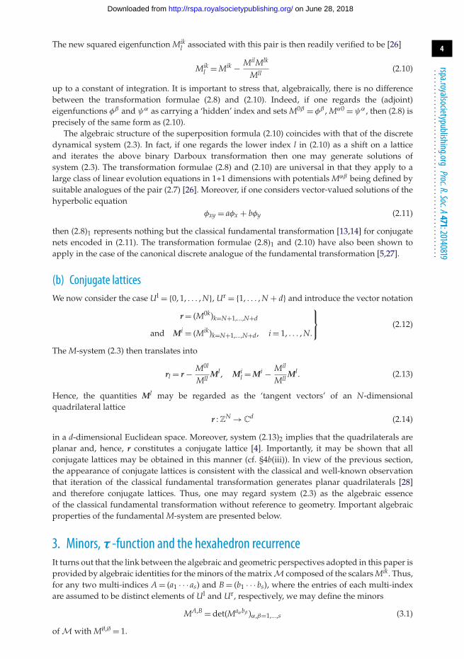
3. Minors, τ -function and the hexahedron recurrenceIt turns out that the link between the algebraic and geometric perspectives adopted in this paper isprovided by algebraic identities for the minors of the matrix M composed of the scalars Mik. Thus,for any two multi-indices A = (a1 · · · as) and B = (b1 · · · bs), where the entries of each multi-indexare assumed to be distinct elements of Ul and Ur, respectively, we may define the minors

MA,B = det(Maαbβ )α,β=1,...,s (3.1)

of M with M∅,∅ = 1.



5


...................................................

(a) Jacobi-type identities and identification of a metricIn terms of the above minors, Jacobi’s classical identity for determinants [29] may be expressed as

MA,BMaaA,bbB − MaA,bBMaA,bB + MaA,bBMaA,bB = 0. (3.2)

A compact form of this quadratic identity is given by

〈Waa,bb,Waa,bb〉 = 0, (3.3)

where

Waa,bb = (MA,B, MaaA,bbB, MaA,bB, MaA,bB, MaA,bB, MaA,bB) (3.4)

and the inner product is taken with respect to the block-diagonal metric

diag

[(0 11 0

), −

(0 11 0

),

(0 11 0

)]. (3.5)

In the above, it is assumed that all upper-left indices and all upper-right indices are distinct sothat the associated minors are well defined.

The identity

MA,BMaaaA,bbbB + MaaA,bbBMaA,bB − MaA,bBMaaA,bbB − MaA,bBMaaA,bbB

+ MaA,bBMaaA,bbB + MaA,bBMaaA,bbB = 0 (3.6)

constitutes an algebraic consequence of the Jacobi identity and proves equally important in thesubsequent analysis. Its validity is readily verified by formulating it as

〈Waa,bb,Waaa,bbb〉 = 0, (3.7)

where

Waaa,bbb = (MaA,bB, MaaaA,bbbB, MaaA,bbB, MaaA,bbB, MaaA,bbB, MaaA,bbB). (3.8)

Indeed, four applications of the Jacobi identity (3.2) show that the vector

�W= MaA,bBWaa,bb − MA,BWaaa,bbb (3.9)

is of the form

�W= (0, ∗, MaA,bBMaA,bB, MaA,bBMaA,bB, MaA,bBMaA,bB, MaA,bBMaA,bB) (3.10)

so that it is seen that

〈�W,�W〉 = 0. (3.11)

The latter is equivalent to (3.7), because Waa,bb and Waaa,bbb are null vectors with respect to themetric (3.5).

A degenerate case of the identity (3.6) is obtained by (temporarily) assuming that the rows ofthe matrix M labelled by a and a are identical. In this case, three of the terms in (3.6) vanish andwe are left with

MaaA,bbBMaA,bB − MaA,bBMaaA,bbB + MaA,bBMaaA,bbB = 0. (3.12)

In the same manner as above, it may now be shown that

〈Waaa,bbb,Waaa,bbb〉 = 0. (3.13)



6


...................................................

Here, (3.12) plays the role of the Jacobi identity (3.2). It is evident that, for reasons of symmetry,the identity

〈Waaa,bbb,Waaa,bbb〉 = 0 (3.14)

likewise holds. The geometric significance of the identities (3.3), (3.7) and (3.13), (3.14) isaddressed in §4.

(b) Evolution of the minors and the τ -functionFor any l ∈ L which is not contained in two multi-indices A and B, a Laplace expansion of MlA,lB

with respect to the row or column labelled by l shows that

MA,Bl = MlA,lB

Ml,l. (3.15)

Hence, if A and B constitute simple indices, then the M-system (2.3) is retrieved. Accordingly,system (2.3) may be reinterpreted as the integrable evolution (3.15) of the minors of the matrix M.It is interesting to note that if one sets aside the genesis of the system (3.15), then (3.15) stillconstitutes a consistent system for some quantities MA,B, because the compatibility condition(MA,B

l )m = (MA,Bm )l is readily seen to be satisfied. Hence, (3.1) may be regarded as a realization

of the quantities MA,B in terms of the minors of a matrix M which evolves according to (2.3).Whether there exist other realizations is the subject of current research.

In the particular case Ul = Ur = L, the above evolution of the minors gives rise to a compactformulation of the evolution of a τ -function associated with the M-system. Thus, it is readilyverified that the compatibility conditions (τi)k = (τk)i, which guarantee the existence of a functionτ defined according to

τi = Miiτ , (3.16)

are satisfied modulo the M-system (2.3). In fact, it turns out that

τik = Mik,ikτ =∣∣∣∣∣M

ii Mik

Mki Mkk

∣∣∣∣∣ τ , (3.17)

which is, indeed, symmetric in the distinct indices i and k. In general, if we consider the multi-index A = (a1 · · · aα) with distinct entries, then the evolution (3.15) immediately implies that

τA = MA,Aτ . (3.18)

In particular, three distinct unit increments result in

τikl =

∣∣∣∣∣∣∣Mii Mik Mil

Mki Mkk Mkl

Mli Mlk Mll

∣∣∣∣∣∣∣ τ . (3.19)

It is noted that any binary Darboux transformation (continuous or discrete) which admits thesuperposition principle (2.10) gives rise to determinantal formulae of the above type if theapplication of a binary Darboux transformation is regarded as a shift on a lattice [30–32].

(c) The hexahedron recurrenceWe conclude this section with an application of the τ -function. A so-called hexahedron recurrencehas been proposed by Kenyon & Pemantle [15] which admits a natural interpretation in terms



7


...................................................

of cluster algebras and dimer configurations [33]. Here, it is demonstrated that the hexahedronrecurrence is but another avatar of the M-system for Ul = Ur = L = {1, 2, 3}. Thus, four functions

h, hx, hy, hz : Z3 → C (3.20)

are said to satisfy the hexahedron recurrence if these are solutions of the coupled system ofdifference equations

hx1hxh = hxhyhz + h1h2h3 + hh1h23,

hy2hyh = hxhyhz + h1h2h3 + hh1h13,

hz3hzh = hxhyhz + h1h2h3 + hh1h12

and h123h2hxhyhz = (hxhyhz)2 + hxhyhz(2h1h2h3 + hh1h23 + hh2h13 + hh3h12)

+ (h1h2 + hh12)(h1h3 + hh13)(h2h3 + hh23).

⎫⎪⎪⎪⎪⎪⎪⎪⎪⎪⎬⎪⎪⎪⎪⎪⎪⎪⎪⎪⎭

(3.21)

We now introduce the quantities

�x = h2h3 + hh23, �y = h1h3 + hh13, �z = h1h2 + hh12, (3.22)

which are seen to constitute key components in the system (3.21). In particular, the third-orderequation (3.21)4 may be cast in the form

h123

h= hxhyhz

h3 + h1�x

h3 + h2�y

h3 + h3�z

h3 − h1h2h3

h3 + �x�y�z

h3hxhyhz , (3.23)

which suggests that its right-hand side may be written as a 3×3 determinant. Accordingly, wemake the change of variables

M23 = −hx

h, M31 = −hy

h, M12 = −hz

h(3.24)

and express one and two distinct unit increments of the arguments of h in terms of the functions

M11 = h1

h, M22 = h2

h, M33 = h3

h(3.25)

and

M32 = −�x

hhx , M13 = −�y

hhy , M21 = −�z

hhz , (3.26)

respectively. The latter two sets of relations may be formulated as

hi = Miih, hik = −∣∣∣∣∣M

ii Mik

Mki Mkk

∣∣∣∣∣ h, (3.27)

and the hexahedron recurrence relation (3.23) becomes

h123 = −

∣∣∣∣∣∣∣M11 M12 M13

M21 M22 M23

M31 M32 M33

∣∣∣∣∣∣∣ h. (3.28)

On use of the definitions (3.24), the remaining hexahedron recurrence relations (3.21)1,2,3 may bewritten as

M231 = M32 − M31M12

M11 (3.29)

and its analogues obtained by cyclically interchanging the indices. Moreover, comparison of(3.27)1 shifted in the direction nk and (3.27)2 yields

Miik = −Mii + MikMki

Mkk, (3.30)



8


...................................................

whereas (3.27)2 shifted in the direction nl, l �= i, k and matched with (3.28) produces

M321 = M23 − M21M13

M11 (3.31)

and its two counterparts. Hence, the functions Mik evolve according to

Mikl = Mki − MklMli

Mll, i �= k �= l �= i. (3.32)

Finally, if the ‘transposition’ operator C is defined by

CMik = Mki, (3.33)

then the successive change of variables

Mik → CnMik, n = n1 + n2 + n3

Mik → (−1)ni+nk Mik, (i, k) ∈ {(1, 2), (2, 3), (3, 1)}and Mii → (−1)nk+nl Mii, i �= k �= l �= i

⎫⎪⎪⎪⎬⎪⎪⎪⎭

(3.34)

transforms the system (3.30), (3.32) into the M-system (2.3) for Ul = Ur = L = {1, 2, 3} and thefunction

τ = (−1)n1n2+n2n3+n3n1 h (3.35)

constitutes the corresponding τ -function obeying the linear system (3.16) and its higher-orderimplications (3.17) and (3.19).

One of the intriguing properties of the hexahedron recurrence (3.21) is that the solution remainspositive if the initial data are positive. Unfortunately, this important property is hidden in theM-system avatar. However, the advantage of the latter formulation is that multi-dimensionalconsistency is automatically guaranteed. In this connection, it is noted that the cube recurrence,that is, the discrete BKP (Miwa) equation, may be formulated in such a manner that positivity isguaranteed but this property does not hold on higher-dimensional lattices [34].

The hexahedron recurrence admits a reduction to a single third-order ‘recurrence’ obtainedby Kashaev [35] in the context of star-triangle moves in the Ising model. The existence of thisrecurrence is readily verified if one exploits its formulation in terms of the M-system. Indeed, itis evident that the M-system considered above admits the reduction Mik = Mki corresponding toa symmetric matrix M. Elimination of its entries Mik between the linear system (3.17) and (3.19)has been shown to lead to the discrete CKP (dCKP) equation [36]

(ττ123 + τ1τ23 − τ2τ13 − τ3τ12)2 − 4(τ12τ13 − τ1τ123)(τ2τ3 − ττ23) = 0. (3.36)

By construction, the left-hand side is symmetric in the indices and, remarkably, turns out tobe Cayley’s 2 × 2 × 2 hyperdeterminant [37]. Furthermore, the dCKP equation interpreted asa local relation between the principal minors of a symmetric matrix M has been derived asa characteristic property by Holtz & Sturmfels [16] in connection with the ‘principal minorassignment problem’. This remarkable interpretation naturally places this equation on a multi-dimensional lattice and implies its multi-dimensional consistency [38].

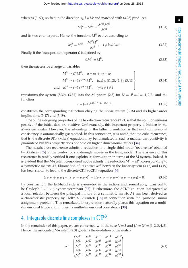
4. Integrable discrete line complexes inCP3

In the remainder of this paper, we are concerned with the case N = 3 and Ul = Ur = {1, 2, 3, 4, 5}.Hence, the associated M-system (2.3) governs the evolution of the matrix

M=

⎛⎜⎜⎜⎜⎜⎝

M11 M12 M13 M14 M15

M21 M22 M23 M24 M25

M31 M32 M33 M34 M35

M41 M42 M43 M44 M45

M51 M52 M53 M54 M55

⎞⎟⎟⎟⎟⎟⎠ (4.1)



9


...................................................

as a function of n1, n2, n3. More precisely, if we prescribe the Cauchy data

Mik(Sik), Sik = {(n1, n2, n3) : nl = 0, l �∈ {i, k}} (4.2)

at the origin and on appropriate coordinate lines and planes Sik, then M is uniquely determinedby the evolution equations (2.3).

(a) From algebra to geometryIn order to reveal the geometry encoded in the matrix M, we focus on the submatrix

M=(

M44 M45

M54 M55

), (4.3)

which is uniquely determined by its value at the origin and the Cauchy data associated with theremaining matrix entries.

(i) Identification of a Plücker quadric

If we define the vector-valued function

V= (M∅,∅, M45,45, M4,4, M5,5, M5,4, M4,5), (4.4)

which is composed of all minors of the matrix M, then the functional relationship

M∅,∅M45,45 − M4,4M5,5 + M5,4M4,5 = 0 (4.5)

between these minors may be expressed as

〈V, V〉 = 0. (4.6)

The latter elementary identity is a special case of the Jacobi identity (3.3), wherein A = B = ∅ and(a, a) = (b, b) = (4, 5). By virtue of the signature of the metric (3.5), it is therefore natural to regard Vas a function

V : Z3 → C

3,3, (4.7)

which represents particular homogeneous coordinates of a lattice of points in a four-dimensionalquadric Q4 embedded in a five-dimensional complex projective space P(C3,3). If we identify thequadric Q4 with the complexification of the classical Plücker quadric [18] then, on use of thePlücker correspondence (cf. §4b(i)), we may interpret any point [V(n)] ∈ Q4 as a line l(n) ⊂ CP

3 ina three-dimensional complex projective space. Here, [X] ∈ P(C3,3) refers to a point in projectivespace with associated homogeneous coordinates X ∈ C

3,3. Accordingly, V may be identified with a(discrete) line complex

l : Z3 → {lines in CP

3}, (4.8)

that is, a three-parameter family of lines which are combinatorially attached to the vertices of Z3

as indicated schematically in figure 1.

(ii) Incidence of lines

In order to uncover the geometric properties of the line complex l defined by V, we first observethat a shift of V in any lattice direction may be expressed elegantly in terms of higher-order minors



10


...................................................

13

233

123

2

121

Figure 1. A combinatorial picture of a line complex l which admits the ‘intersection property’. The lines are combinatoriallyattached to the vertices of a Z

3 lattice. Any two neighbouring lines intersect in a point which may be associated with thecorresponding edge.

ml

l

m

l

mm,l

l,mlm

lm

Figure 2. The relationship between the lines l, the points of intersection pl and the diagonals lm,p.

of M. Indeed, ‘raising indices’ by means of the identity (3.15) produces

Vl = (Ml,l, Ml45,l45, Ml4,l4, Ml5,l5, Ml5,l4, Ml4,l5)Ml,l

(4.9)

so that setting A = B = ∅ and (a, a, a) = (b, b, b) = (l, 4, 5) in (3.7) yields

〈Vl, V〉 = 0. (4.10)

In geometric terms, this orthogonality condition expresses the fact that the associated lines l andll intersect. Thus, the line complex l has the property that the two lines which are combinatoriallyattached to the two vertices of any edge of Z

3 intersect as depicted in figure 1.The above geometric property implies that the four lines l, ll, lm and llm with l �= m form a (skew)

quadrilateral (figure 2). Its diagonals ll,m and lm,l may be obtained by solving the linear system

〈V∗,∗, V〉 = 〈V∗,∗, Vl〉 = 〈V∗,∗, Vm〉 = 〈V∗,∗, Vlm〉 = 0 (4.11)

subject to the condition 〈V∗,∗, V∗,∗〉 = 0. On raising indices by means of (3.15), this linear systemmay be formulated as

〈V∗,∗, V〉 = 〈V∗,∗, Vl,l〉 = 〈V∗,∗, Vm,m〉 = 〈V∗,∗, Vlm,lm〉 = 0, (4.12)

whereVC,D = (MC,D, MC45,D45, MC4,D4, MC5,D5, MC5,D4, MC4,D5) (4.13)

for any multi-indices C and D such that the relevant minors are well defined. Up to scaling, thetwo null vector solutions turn out to be

Vl,m, Vm,l. (4.14)



11


...................................................

231

3

31

213

21

3

2

3

1

13

123

12

2

1

23

32

12

123

312

Figure 3. A combinatorial picture of a fundamental line complex l. The four points of intersection attached to any four edgesof the same ‘type’ are coplanar. This is equivalent to the concurrency of any four ‘diagonals’ of the same ‘type’ indicated by thedotted lines.

Indeed, for instance, the identity (3.7) for (a, a) = (b, b) = (4, 5) and a = l, b = m with A = B = ∅ anda = m, b = l with A = l, B = m coincides with 〈Vl,m, V〉 = 0 and 〈Vl,m, Vlm,lm〉 = 0, respectively. On theother hand, 〈Vl,m, Vl,l〉 = 0 due to the identity (3.13) for (a, a) = (b, b) = (4, 5) and a = l, b = l, b = mwith A = B = ∅. Similarly, the remaining vanishing inner product 〈Vl,m, Vm,m〉 = 0 is a consequenceof the identity (3.14). Finally, for reasons of symmetry, the same arguments apply in the case ofthe solution Vm,l.

(iii) Coplanarity and concurrency properties

In order to analyse the properties of the diagonals ll,m, we label the points of intersection of anytwo neighbouring lines by

[pl] = l ∩ ll (4.15)

and state the following lemma, which is proven in §4b. It is noted that, for brevity, we make nodistinction between a point of intersection [pl] ∈ CP

3 and its (particular) homogeneous coordinatespl ∈ C

4 whenever this cannot lead to any confusion.

Lemma 4.1. The diagonal ll,m passes through the points of intersection pl and plm.

It is natural to associate the point of intersection of any two neighbouring lines with the edgeconnecting the corresponding vertices of the Z

3 lattice. Thus, if we consider four edges of the same‘type’ of an elementary cube then, according to lemma 4.1, the associated points of intersection

pl, plm, pl

p and plmp may be regarded as the vertices of a quadrilateral with edges ll,m, ll,p and ll,mp , ll,pm

(cf. figure 3). Remarkably, this quadrilateral is planar because, for instance, the lines ll,m and ll,mpintersect, as may be concluded from

〈Vl,m, Vl,mp 〉 ∼ 〈Vl,m, Vpl,pm〉 = 0 (4.16)

by virtue of the identity (3.7). Furthermore, because the lines ll,m and lp,m lie in the plane spannedby the lines l and lm, the former lines likewise intersect. Algebraically, this is confirmed by

〈Vl,m, Vp,m〉 = 0, (4.17)



12


...................................................

which, once again, constitutes a special case of the identity (3.14). In fact, it is evident that, underappropriate genericity assumptions, the four diagonals of the same ‘type’ ll,m, ll,mp and lp,m, lp,m

lmust be concurrent, as indicated in figure 3. Hence, we are led to privileged line complexes whichhave been termed rectilinear congruences in [5]. In the current context, we adopt the followingterminology.

Definition 4.2. A line complex l : Z3 → {lines in CP

3} is termed fundamental if any neighbouringlines l and ll intersect and the points of intersection pl enjoy the coplanarity property, that is, forany distinct l, m and p, the quadrilaterals (pl, pl

m, plmp, pl

p) are planar. Equivalently, the lines passing

through the points pl and plm admit the concurrency property, that is, the four lines connecting the

points pl, pp, plp, pp

l and their shifted counterparts plm, pp

m, plpm, pp

lm are concurrent.

Remark 4.3. It is readily verified that if any one of the six coplanarity and concurrencyconditions associated with an elementary cube of a line complex is satisfied then the other fiveconditions automatically hold.

The analysis presented in the preceding may therefore be summarized as follows.

Theorem 4.4. Any solution M of the M-system (2.3) with N = 3 and Ul = Ur = {1, 2, 3, 4, 5}parametrizing a function V according to (4.4) encapsulates a fundamental line complex l via the Plückercorrespondence V↔ l.

(b) From geometry to algebraHere, we demonstrate that the converse of theorem 4.4 is also true, that is, all fundamental linecomplexes are algebraically represented by the M-system (2.3).

(i) The Plücker correspondence

The classical Plücker correspondence is established by considering a lift a ∧ b of a line l in CP3,

that is, by introducing homogeneous coordinates

a=

⎛⎜⎜⎜⎝α0

α1

α2

α3

⎞⎟⎟⎟⎠ , b=

⎛⎜⎜⎜⎝β0

β1

β2

β3

⎞⎟⎟⎟⎠ (4.18)

of two points on the line l and setting

V= (γ 01, γ 23, γ 02, γ 13, γ 03, γ 12), (4.19)

where the coefficients γ μν are defined by the subdeterminants

γ μν = det

(αμ βμ

αν βν

). (4.20)

It is easy to verify that the γ μν obey the classical Plücker identity

γ 01γ 23 − γ 02γ 13 + γ 03γ 12 = 0 (4.21)

so that the components of V, indeed, constitute homogeneous coordinates of a point in the Plückerquadric Q4. Specifically, in the generic case, we may make the choice

a=

⎛⎜⎜⎜⎝

01

M44

M54

⎞⎟⎟⎟⎠ , b=

⎛⎜⎜⎜⎝

−10

M45

M55

⎞⎟⎟⎟⎠ (4.22)

so that

V=(

1,

∣∣∣∣∣M44 M45

M54 M55

∣∣∣∣∣ , M44, M55, M54, M45

)(4.23)



13


...................................................

is precisely of the form (4.4). However, at this stage, M44, M55, M54 and M45 are merely labels ofthe ‘non-trivial’ homogeneous coordinates of the points a and b.

We now focus on the lines of a fundamental line complex l. Because any neighbouring lines land ll intersect, the points a, b and al, bl must be coplanar. This may be expressed as

Nl5�la= Nl4�lb (4.24)

due to the constancy of the first two components of a and b. Here, Nl4 and Nl5 are functions to bedetermined and �lf = fl − f . Accordingly, the points of intersection pl are given by

pl = Nl5a − Nl4b. (4.25)

As an illustration, we (temporarily) consider a fundamental line complex parametrized by asolution of the M-system as stated in theorem 4.4. In this case, the evolution of the matrix (4.3)may be formulated as

�la= −Ml4

MllMl, �lb= −Ml5

MllMl, Ml =

⎛⎜⎜⎜⎝

00

M4l

M5l

⎞⎟⎟⎟⎠ (4.26)

so that

pl ∼ Ml5a − Ml4b=

⎛⎜⎜⎜⎝

Ml4

Ml5

Ml5M44 − Ml4M45

Ml5M54 − Ml4M55

⎞⎟⎟⎟⎠=

⎛⎜⎜⎜⎝

Ml,4

Ml,5

Ml4,54

Ml5,54

⎞⎟⎟⎟⎠ . (4.27)

On use of the Plücker correspondence (4.18)–(4.20) and the identities of §3a, it is thenstraightforward to verify that the line passing through the points of intersection pl and pl

m is indeedgiven by the diagonal ll,m as stated in lemma 4.1.

(ii) Fundamental line complexes inCP4

In order to make the transition from a fundamental line complex to a solution of the M-system, we first observe that, as pointed out in [5], the inclusion of the coplanarity property or,equivalently, the concurrency property in the definition of a fundamental line complex is due tothe dimensionality of the ambient space of the line complexes discussed here. Thus,

Definition 4.5. A line complex l : Z3 → {lines in CP

4} is termed fundamental if any neighbouringlines l and ll intersect.

Indeed, the two sets of four lines {l, l1, l2, l12} and {l3, l13, l23, l123} span two (three-dimensional)hyperplanes which, generically, intersect in a (two-dimensional) plane. The latter plane containsthe points p3, p3

1, p32, p3

12, so that the set of points p3 automatically enjoys the coplanarity property.It turns out that fundamental line complexes in CP

3 may be regarded as projections offundamental line complexes in CP

4.

Theorem 4.6. A line complex in CP3 is fundamental if and only if it may be regarded as a projection

onto a hyperplane of a fundamental line complex in CP4.

Proof. Given a fundamental line complex in CP3 which we regard as being embedded in a

hyperplane of CP4, we consider an ‘elementary cube’ of eight lines l, . . . , l123 and associated points

of intersection. We begin by choosing a generic projection π and prescribing five (black) pointsp2

3, p32, p1

2, p21, p3

1 such that π (plm) = pl

m for (l, m) �= (1, 3) as depicted in figure 4. These points definethe four lines l23, l2, l12, l1 which project onto the lines l23, l2, l12, l1, respectively. Because [p1] ∈ l1and [p2] ∈ l2, the lines l1 and l2 uniquely determine the (grey) points p1 and p2 lying on l1 and

l2, respectively, and obeying π (p1) = p1 and π (p2) = p2. The line l passing through p1 and p2 andprojecting onto the line l gives rise, in turn, to the point p3 (grey square) lying on l such that



14


...................................................

3

1

ˆ

ˆ

ˆˆ

2

ˆ13

ˆ1 ˆ

12

ˆ2

ˆ23

ˆ123

ˆ

ˆ3

13

31

ˆ

ˆ

12ˆ

32ˆ

23

ˆ 21

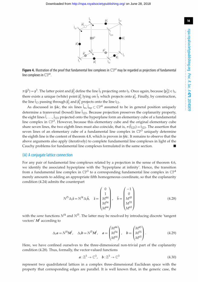
Figure 4. Illustration of the proof that fundamental line complexes inCP3 may be regarded as projections of fundamental

line complexes inCP4.

π (p3) = p3. The latter point and p23 define the line l3 projecting onto l3. Once again, because [p1

3] ∈ l3,there exists a unique (white) point p1

3 lying on l3 which projects onto p13. Finally, by construction,

the line l13 passing through p13 and p3

1 projects onto the line l13.As discussed in §4c, the six lines lm, lmp ⊂ CP

4 assumed to be in general position uniquelydetermine a transversal (boxed) line l123. Because projection preserves the coplanarity property,the eight lines l, . . . , l123 projected onto the hyperplane form an elementary cube of a fundamentalline complex in CP

3. However, because this elementary cube and the original elementary cubeshare seven lines, the two eighth lines must also coincide, that is, π (l123) = l123. The assertion thatseven lines of an elementary cube of a fundamental line complex in CP

3 uniquely determinethe eighth line is the content of theorem 4.8, which is proven in §4c. It remains to observe that theabove arguments also apply (iteratively) to complete fundamental line complexes in light of theCauchy problems for fundamental line complexes formulated in the same section. �

(iii) A conjugate lattice connection

For any pair of fundamental line complexes related by a projection in the sense of theorem 4.6,we identify the associated hyperplane with the ‘hyperplane at infinity’. Hence, the transitionfrom a fundamental line complex in CP

3 to a corresponding fundamental line complex in CP4

merely amounts to adding an appropriate fifth homogeneous coordinate, so that the coplanaritycondition (4.24) admits the counterpart

Nl5�l a= Nl4�lb, a=

⎛⎜⎜⎜⎜⎜⎝

01

M44

M54

M64

⎞⎟⎟⎟⎟⎟⎠ , b=

⎛⎜⎜⎜⎜⎜⎝

−10

M45

M55

M65

⎞⎟⎟⎟⎟⎟⎠ (4.28)

with the same functions Nl4 and Nl5. The latter may be resolved by introducing discrete ‘tangentvectors’ Ml according to

�la = Nl4Ml, �lb = Nl5Ml, a =

⎛⎜⎝M44

M54

M64

⎞⎟⎠ , b =

⎛⎜⎝M45

M55

M65

⎞⎟⎠ . (4.29)

Here, we have confined ourselves to the three-dimensional non-trivial part of the coplanaritycondition (4.28). Thus, formally, the vector-valued functions

a : Z3 → C

3, b : Z3 → C

3 (4.30)

represent two quadrilateral lattices in a complex three-dimensional Euclidean space with theproperty that corresponding edges are parallel. It is well known that, in the generic case, the



15


...................................................

quadrilaterals of lattices of this type must be planar and, hence, by definition, the conjugatelattices a and b constitute Combescure transforms of each other [39].

The planarity of the quadrilaterals of a and b may be expressed as

Mlm = ImlMl + NmlMm, l �= m (4.31)

with associated compatibility conditions (Mlm)p = (Ml

p)m

, leading to

Imlp (IplMl + NplMp) + Nml

p (IpmMm + NpmMp)

= Iplm(ImlMl + NmlMm) + Npl

m(ImpMp + NmpMm). (4.32)

Under the non-degeneracy assumption of linearly independent tangent vectors M1, M2, M3, wetherefore conclude that, in particular,

Imlp Ipl = Ipl

mIml. (4.33)

It is observed that these relations may be interpreted as the algebraic incarnation of theorem 4.6.Thus, if the vectors Ml were associated with a line complex in CP

3 and therefore two-dimensionalthen the expansions (4.31) would still be valid but equating to zero and then the coefficientsmultiplying the tangent vectors in (4.32) would not be justified. The conditions (4.33) give riseto the parametrization

Iml = ϕlm

ϕl(4.34)

in terms of potentials ϕl. These may be used to scale the coefficients Iml to unity by applying thegauge transformation Ml → ϕlMl. Hence, we may assume without loss of generality that Iml = 1.The remaining compatibility conditions then reduce to the nonlinear system

Nmlp = Nml + NmpNpl

1 − NmpNpm . (4.35)

The latter constitutes a standard discretization of the classical Darboux equations governingequivalence classes of Combescure transforms of conjugate coordinate systems [40,41]. Forany fixed solution Nlm, Ml of the discrete Darboux system and the linear system (4.31), twoCombescure transforms are given by a and b, where the coefficients Nl4 and Nl5 are solutionsof the same linear system

Nlkm = Nlk + NlmNmk

1 − NlmNml, k = 4, 5, (4.36)

namely the compatibility conditions associated with the linear system (4.29). It is noted that thetwo systems (4.35) and (4.36) are identical in form.

The final step in the identification of the M-system in question is based on the observation thatthe discrete Darboux system admits the ‘conservation laws’

Ξ lmΞlpm =Ξ lpΞ lm

p , Ξ lm = 1 − NlmNml. (4.37)

Accordingly, there exist associated potentials Mll defined by the linear equations

Mllm = (1 − NlmNml)Mll. (4.38)

Hence, if we introduce the parametrization

Nlm = −Mlm

Mll, Ml =

⎛⎜⎝M4l

M5l

M6l

⎞⎟⎠ (4.39)

then the systems (4.29), (4.31), (4.35), (4.36) and (4.38) may be combined to obtain the M-system


Mll, l �∈ {i, k}

and i ∈ {1, 2, 3, 4, 5, 6}, k ∈ {1, 2, 3, 4, 5}, l ∈ {1, 2, 3}.

⎫⎪⎬⎪⎭ (4.40)



16


...................................................

(a) (b)

Figure 5. (a) Six (black) lines forming a spatial hexagon uniquely determine the remaining two (boxed) lines of an ‘elementarycube’ of a fundamental line complex inCP

4. (b) A Cauchy problem for fundamental line complexes. InCP4, the boxed lines are

determined by the black lines. InCP3, the boxed lines constitute additional Cauchy data which have to intersect the relevant

triples of black lines.

Because the coefficients M6k are merely auxiliary functions which represent the transition of afundamental line complex from CP

3 to CP4, we are now in a position to state the converse of

theorem 4.4.

Theorem 4.7. Any fundamental line complex in CP3 gives rise to a solution M of the M-system (2.3)

with N = 3 and Ul = Ur = {1, 2, 3, 4, 5} via the lift a ∧ b of the lines l encapsulated in (4.22).

(c) Geometric construction of fundamental line complexesAn elementary cube of a fundamental line complex l in CP

4 may be constructed by prescribing askew hexagon formed by the two triples of lines l1, l2, l3 and l12, l23, l13 (figure 5). On the assumptionthat these triples are in general position, the lines l and l123 are then uniquely determined bythe requirement that these pass through the relevant triple of lines. An entire fundamental linecomplex is uniquely determined by prescribing a ‘plane’ of hexagons as Cauchy data, that is, byspecifying the set of lines

{l(n1, n2, n3) : n1 + n2 + n3 ∈ {1, 2}} (4.41)

as illustrated in figure 5.In the case of fundamental line complexes in CP

3, the Cauchy problem becomes non-trivial,because the coplanarity property needs to be taken into account. If we prescribe a hexagon of linesas above then the three lines l1, l2, l3 may be interpreted as three generators of a unique quadric.The line l then constitutes an element of the second one-parameter family of generators of thequadric. An analogous interpretation is valid in the case of the second triple of lines l12, l23, l13 andits transversal line l123. As shown in [5], the line l123 is uniquely determined by the coplanarityproperty and a fixed choice of the line l. In fact, the existence of the line l123 may be traced back tothe classical Desargues theorem of projective geometry [19].

Theorem 4.8. Given seven lines in CP3 which are combinatorially attached to seven vertices of an

elementary cube and intersect each other ‘along edges’, there exists a unique eighth line such that the eightlines constitute an elementary cube of a fundamental line complex.

Proof. Without loss of generality, we consider the seven (short black) lines l, l1, l2, l3 and l12, l23, l13depicted in figure 6. The associated nine (black) points of intersection are given by p1, p1

2, p13,

p2, p21, p2

3 and p3, p31, p3

2. The coplanarity property is implemented by defining p312 as the (grey) point

of intersection of the plane passing through p3, p31, p3

2 and the line l12. Similarly, the (grey) points p123

and p213 are constructed. In order to demonstrate that the three points p1

23, p213 and p3

12 are indeedcollinear and therefore define the (boxed) line l123, we focus on a subset of nine lines, namely,for instance, the lines l1, l12, l13 and the lines passing through the pairs of points of intersection(p1, p1

2), (p13, p1

23), (p31, p3

12) and (p1, p13), (p1

2, p123), (p2

1, p213) (cf. figure 7). Because the coplanarity property



17


...................................................

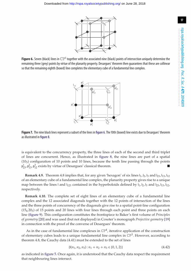
Figure 6. Seven (black) lines inCP3 together with the associated nine (black) points of intersection uniquely determine the

remaining three (grey) points by virtue of the planarity property. Desargues’ theorem then guarantees that these are collinearso that the remaining eighth (boxed) line completes the elementary cube of a fundamental line complex.

13

31

21

213

312

123

13

12

1

1 12

123

Figure 7. The nine black lines represent a subset of the lines in figure 6. The 10th (boxed) line exists due to Desargues’ theoremas illustrated in figure 8.

is equivalent to the concurrency property, the three lines of each of the second and third tripletof lines are concurrent. Hence, as illustrated in figure 8, the nine lines are part of a spatial(103) configuration of 10 points and 10 lines, because the tenth line passing through the pointsp1

23, p213, p3

12 exists by virtue of Desargues’ classical theorem. �

Remark 4.9. Theorem 4.8 implies that, for any given ‘hexagon’ of six lines l1, l2, l3 and l23, l13, l12of an elementary cube of a fundamental line complex, the planarity property gives rise to a uniquemap between the lines l and l123 contained in the hyperboloids defined by l1, l2, l3 and l23, l13, l12,respectively.

Remark 4.10. The complete set of eight lines of an elementary cube of a fundamental linecomplex and the 12 associated diagonals together with the 12 points of intersection of the linesand the three points of concurrency of the diagonals give rise to a spatial point-line configuration(154 203) of 15 points and 20 lines with four lines through each point and three points on eachline (figure 9). This configuration constitutes the frontispiece to Baker’s first volume of Principlesof geometry [20] and was used (but not displayed) in Coxeter’s monograph Projective geometry [19]in connection with the proof of the converse of Desargues’ theorem.

As in the case of fundamental line complexes in CP4, iterative application of the construction

of elementary cubes leads to a unique fundamental line complex in CP3. However, according to

theorem 4.8, the Cauchy data (4.41) must be extended to the set of lines

{l(n1, n2, n3) : n1 + n2 + n3 ∈ {0, 1, 2}} (4.42)

as indicated in figure 5. Once again, it is understood that the Cauchy data respect the requirementthat neighbouring lines intersect.



18


...................................................

1

1

13

12312

123

213

312

31

13

21

12

Figure 8. The Desargues configuration associated with the 10 lines of the fundamental line complex displayed in figure 7. Thetwo white points exist due to the concurrency property.

Figure9. Aclassical (154 203) point-line configurationwhich is characterizedby theproperty that three triangles areperspectivefrom three collinear points or, equivalently, from a line.

5. Fundamental line complexes and correlationsIt turns out that fundamental line complexes in CP

3 may be characterized in terms of correlations.A correlation of a d-dimensional projective space is an incidence-preserving transformation whichmaps k-dimensional projective subspaces to d − k − 1-dimensional projective subspaces [18,22].In particular, in three dimensions, the points of a line are mapped to planes which meet in a line.Here, we represent a correlation by a map

κ : CP3 → {planes in CP

3}. (5.1)

For brevity, we use the same symbol κ for the representation of this map in terms of homogeneouscoordinates. Any correlation is then encoded in a complex 4×4 matrix B such that

κ(x) = {y ∈ C4 : yTBx= 0}. (5.2)

In the previous section, it has been demonstrated that, for any given line of an elementarycube of a fundamental line complex in CP

3, the ‘opposite’ line is determined by the hexagonformed by the remaining six lines and the planarity property. It is therefore natural to enquire asto whether opposite lines of an elementary cube of a fundamental line complex are linked by a



19


...................................................

common correlation. To this end, we recall the self-polarity of a hexagon in CP3 (cf. [23]). Thus,

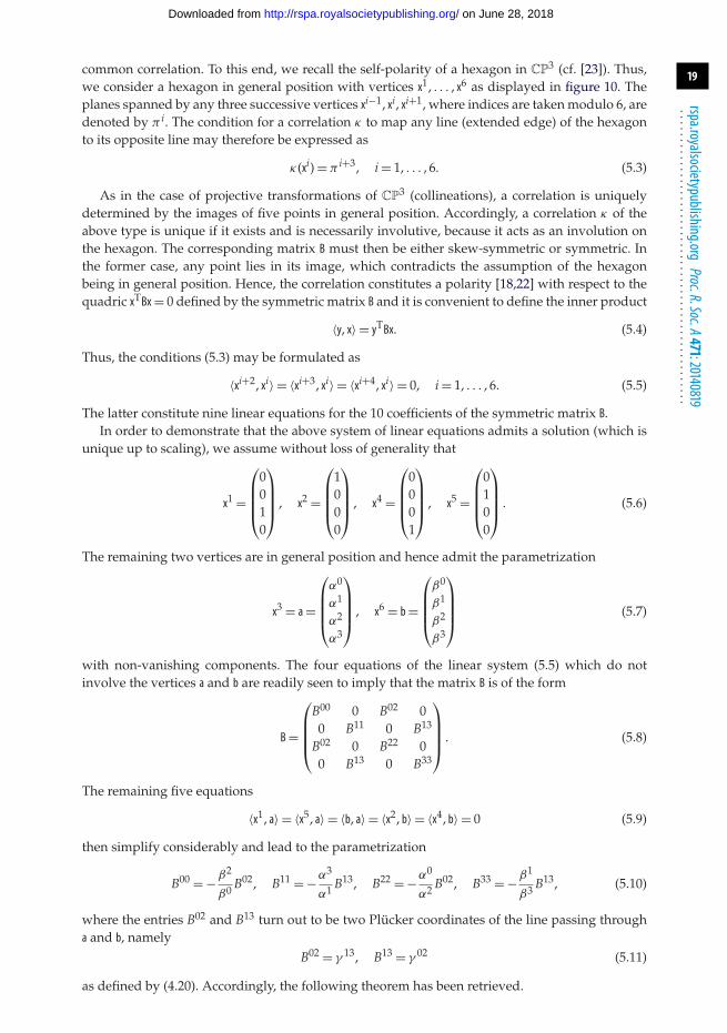
we consider a hexagon in general position with vertices x1, . . . , x6 as displayed in figure 10. Theplanes spanned by any three successive vertices xi−1, xi, xi+1, where indices are taken modulo 6, aredenoted by π i. The condition for a correlation κ to map any line (extended edge) of the hexagonto its opposite line may therefore be expressed as

κ(xi) = π i+3, i = 1, . . . , 6. (5.3)

As in the case of projective transformations of CP3 (collineations), a correlation is uniquely

determined by the images of five points in general position. Accordingly, a correlation κ of theabove type is unique if it exists and is necessarily involutive, because it acts as an involution onthe hexagon. The corresponding matrix B must then be either skew-symmetric or symmetric. Inthe former case, any point lies in its image, which contradicts the assumption of the hexagonbeing in general position. Hence, the correlation constitutes a polarity [18,22] with respect to thequadric xTBx= 0 defined by the symmetric matrix B and it is convenient to define the inner product

〈y, x〉 = yTBx. (5.4)

Thus, the conditions (5.3) may be formulated as

〈xi+2, xi〉 = 〈xi+3, xi〉 = 〈xi+4, xi〉 = 0, i = 1, . . . , 6. (5.5)

The latter constitute nine linear equations for the 10 coefficients of the symmetric matrix B.In order to demonstrate that the above system of linear equations admits a solution (which is

unique up to scaling), we assume without loss of generality that

x1 =

⎛⎜⎜⎜⎝

0010

⎞⎟⎟⎟⎠ , x2 =

⎛⎜⎜⎜⎝

1000

⎞⎟⎟⎟⎠ , x4 =

⎛⎜⎜⎜⎝

0001

⎞⎟⎟⎟⎠ , x5 =

⎛⎜⎜⎜⎝

0100

⎞⎟⎟⎟⎠ . (5.6)

The remaining two vertices are in general position and hence admit the parametrization

x3 = a=

⎛⎜⎜⎜⎝α0

α1

α2

α3

⎞⎟⎟⎟⎠ , x6 = b=

⎛⎜⎜⎜⎝β0

β1

β2

β3

⎞⎟⎟⎟⎠ (5.7)

with non-vanishing components. The four equations of the linear system (5.5) which do notinvolve the vertices a and b are readily seen to imply that the matrix B is of the form

B=

⎛⎜⎜⎜⎝

B00 0 B02 00 B11 0 B13

B02 0 B22 00 B13 0 B33

⎞⎟⎟⎟⎠ . (5.8)

The remaining five equations

〈x1, a〉 = 〈x5, a〉 = 〈b, a〉 = 〈x2, b〉 = 〈x4, b〉 = 0 (5.9)

then simplify considerably and lead to the parametrization

B00 = −β2

β0 B02, B11 = −α3

α1 B13, B22 = −α0

α2 B02, B33 = −β1

β3 B13, (5.10)

where the entries B02 and B13 turn out to be two Plücker coordinates of the line passing througha and b, namely

B02 = γ 13, B13 = γ 02 (5.11)

as defined by (4.20). Accordingly, the following theorem has been retrieved.



20


...................................................

4

2

1

5p 4

6 =

= 3

Figure 10. A hexagon inCP3 with vertices xi and associated planesπ i .

4

3

2

2345

56

61

61

6

534

12

1

4534

¢

23

12

56

Figure 11. The hexagonwith vertices xi uniquely determines a correlationκ which interchanges opposite lines lii+1 and li+3i+4.The correlation κ then maps the given line l to a line l′. The vertices xi and the points of intersection xii+1 enjoy the planarityproperty, that is, for instance, the points x2, x34, x5 and x61 are coplanar.

Theorem 5.1. For any hexagon in CP3 in general, position, there exists a unique correlation which maps

any line (extended edge) of the hexagon to its opposite line. The correlation is involutive and constitutes apolarity.

We now combinatorially attach the lines of the hexagon to six vertices of an elementary cubeand the points of intersection xi to the corresponding edges as depicted in figure 11. The linepassing through the vertices xi and xi+1 is denoted by lii+1. There exists a one-parameter family oflines l which intersect the lines l12, l34 and l56. Any fixed line l is mapped by the correlation κ to aline l′ which intersects the lines l23, l45 and l61. Accordingly, the eight lines l, l12, l23, l34, l45, l56, l61 andl′ form an elementary cube of a line complex with the usual property of lines intersecting alongedges. On the other hand, as pointed out in the preceding, the hexagon and the line l uniquelydetermine via the planarity property an eighth line l such that the eight lines form an elementarycube of a fundamental line complex. Hence, as indicated above, the connection between the linesl′ and l is now being examined.

We denote by xii+1 the point of intersection of a line l or its counterpart l′ and the line lii+1 asindicated in figure 11. One may construct the one-parameter family of lines l by parametrizing thepoints

x12 =μ1x1 + μ2x2, x34 =μ3x3 + μ4x4, x56 =μ5x5 + μ6x6 (5.12)

and solving the collinearity condition

x12 + x34 + x56 = 0 (5.13)



21


...................................................

for μ3,μ4,μ5,μ6 in terms of μ1 and μ2. A brief calculation reveals that

μ3 = β0μ1 − β2μ2

γ 02 , μ4 = γ 03μ1 − γ 23μ2

γ 02

and μ6 = −α0μ1 − α2μ2

γ 02 , μ5 = γ 01μ1 + γ 12μ2

γ 02 .

⎫⎪⎪⎪⎬⎪⎪⎪⎭

(5.14)

Similarly, the one-parameter family of lines intersecting the lines l23, l45 and l61 may be obtainedon use of the parametrization

x23 = ν2x2 + ν3x3, x45 = ν4x4 + ν5x5, x61 = ν6x6 + ν1x1 (5.15)

of the points of intersection. The collinearity condition

x23 + x45 + x61 = 0 (5.16)

then determines the coefficients ν6, ν1, ν2, ν3 in terms of ν4 and ν5. The latter two parameters arefixed (up to scaling) by the condition that l′ be the image of l under the correlation κ . This isequivalent to demanding that, for instance,

〈x12, x23〉 = 0 (5.17)

and it turns out that νi =μi. Finally, one may directly verify that, for instance,

|x2, x34, x5, x61| = 0 (5.18)

so that the points x2, x34, x5, x61 are seen to be coplanar as indicated in figure 11. This implies that,remarkably, the lines lii+1 and l, l′ form an elementary cube of a fundamental line complex in CP

3

and therefore l′ = l. Hence, a characterization of fundamental line complexes in CP3 in terms of

correlations has been uncovered.

Theorem 5.2. Fundamental line complexes in CP3 are line complexes with the property that

neighbouring lines intersect and opposite lines of any elementary cube are interchanged by a correlationwhich, necessarily, constitutes a polarity. Furthermore, the planarity and concurrency properties associatedwith any elementary cube of a fundamental line complex are interchanged by the correspondingcorrelation in the sense that any four coplanar diagonals are mapped to four concurrent diagonals andvice versa.

6. ConclusionThe superposition principle (2.10) for the squared eigenfunctions Mik associated with binaryDarboux transformations is standard in the algebraic and geometric theory of continuousand discrete integrable systems. In this paper, we interpret this superposition principle as astand-alone discrete integrable system, namely the M-system (2.3), and discuss its algebraicand geometric properties. In order to highlight its universality, we have briefly indicated itsdirect connection with conjugate lattices and the hexahedron recurrence. The main aim of thispaper is to introduce a novel correspondence between the M-system and fundamental linecomplexes represented as lattices in the Plücker quadric. In fact, the Plücker coordinates ofthe lines turn out to be the entries Mik and, more generally, the minors of the matrix M.This point of view is custom-made for a detailed analysis of special fundamental linecomplexes associated with subgeometries. This is the subject of a forthcoming publication.For instance, it is well known that the binary Darboux transformation associated with theCKP hierarchy of integrable equations requires the squared eigenfunctions to be ‘symmetric’.Indeed, it is easy to see that the constraint Mik = Mki is compatible with the M-system. Ingeometric terms, this means that one considers the intersection of the Plücker quadric witha hyperplane, resulting in a three-dimensional quadric which one may identify with theLie quadric of Lie circle geometry. In this manner, the intersecting lines of the fundamental



22


...................................................

line complexes are contained in a linear complex and may be reinterpreted as touching-oriented circles. As a consequence, these circle complexes are governed by the dCKP equationalluded to in §3. An analogous approach is also available in the context of Lie spheregeometry. A key ingredient in the geometric treatment of these special fundamental linecomplexes is the characterization of fundamental line complexes in terms of the correlationsdiscussed in §5.

Author contributions. The authors contributed in an equal manner to all components of the research reported inthis paper.Funding statement. This research was supported by the DFG Collaborative Research Centre SFB/TRR 109Discretization in Geometry and Dynamics and the Australian Research Council (ARC).Conflict of interests. We have no competing interests.

References1. Finikov SP. 1959 Theorie der Kongruenzen. Berlin, Germany: Akademie-Verlag.2. Eisenhart LP. 1960 A treatise on the differential geometry of curves and surfaces. New York, NY:

Dover.3. Doliwa A. 2001 Discrete asymptotic nets and W-congruences in Plücker line geometry. J. Geom.

Phys. 39, 9–29. (doi:10.1016/S0393-0440(00)00070-X)4. Bobenko AI, Suris YB. 2008 Discrete differential geometry. Integrable structure. Graduate Studies

in Mathematics, no. 98. Providence, RI: AMS.5. Doliwa A, Santini PM, Manas M. 2000 Transformations of quadrilateral lattices. J. Math. Phys.

41, 944–990. (doi:10.1063/1.533175)6. Sauer R. 1950 Parallelogrammgitter als Modelle für pseudosphärische Flächen. Math. Z. 52,

611–622. (doi:10.1007/BF02230715)7. Wunderlich W. 1951 Zur Differenzengeometrie der Flächen konstanter negativer Krümmung.

Österreich. Akad. Wiss. Math.-Nat. Kl. S.-B. II 160, 39–77.8. Bobenko A, Pinkall U. 1996 Discrete surfaces with constant negative Gaussian curvature and

the Hirota equation. J. Diff. Geom. 43, 527–611.9. Schief WK. 2003 On the unification of classical and novel integrable surfaces. II. Difference

geometry. Proc. R. Soc. Lond. A 459, 373–391. (doi:10.1098/rspa.2002.1008)10. Schief WK. 2006 On a maximum principle for minimal surfaces and their integrable discrete

counterparts. J. Geom. Phys. 56, 1484–1495. (doi:10.1016/j.geomphys.2005.07.007)11. Bobenko AI, Pottmann H, Wallner J. 2010 A curvature theory for discrete surfaces based on

mesh parallelity. Math. Ann. 348, 1–24. (doi:10.1007/s00208-009-0467-9)12. Wang J, Jiang C, Bompas P, Wallner J, Pottmann H. 2013 Discrete line congruences for shading

and lighting. In SGP ’13 Proc. the Eleventh Eurographics/ACMSIGGRAPH Symp. on GeometryProcessing, pp. 53–62. Aire-la-Ville, Switzerland: The Eurographics Association.

13. Eisenhart LP. 1962 Transformations of surfaces. New York, NY: Chelsea.14. Rogers C, Schief WK. 2002 Darboux and Bäcklund transformations. Geometry and modern

applications in soliton theory. Cambridge Texts in Applied Mathematics. Cambridge, UK:Cambridge University Press.

15. Kenyon R, Pemantle R. 2013 Double-dimers, the Ising model and the hexahedron recurrence.(http://arxiv.org/abs/1308.2998)

16. Holtz O, Sturmfels B. 2007 Hyperdeterminantal relations among symmetric principal minors.J. Algebra 316, 634–648. (doi:10.1016/j.jalgebra.2007.01.039)

17. Plücker J. 1865 On a new geometry of space. Phil. Trans. R. Soc. Lond. A 155, 725–791.(doi:10.1098/rstl.1865.0017)

18. Onishchik AL, Sulanke R. 2006 Projective and Cayley–Klein geometries. Springer Monographs inMathematics. Berlin, Germany: Springer.

19. Coxeter HSM. 1987 Projective geometry, 2nd edn. New York, NY: Springer-Verlag.20. Baker HF. 1922 Principles of geometry. Cambridge, UK: Cambridge University Press.21. Bobenko A, Huhnen-Venedey E, Rörig T. Submitted. Supercyclidic nets .22. Semple JG, Kneebone GT. 1952 Algebra projective geometry. Oxford, UK: Oxford University

Press.23. Carver WB. 1905 On the Cayley–Veronese class of configurations. Trans. Am. Math. Soc. 6,

534–545. (doi:10.1090/S0002-9947-1905-1500727-X)


http://dx.doi.org/doi:10.1016/S0393-0440(00)00070-X

http://dx.doi.org/doi:10.1007/BF02230715

http://dx.doi.org/doi:10.1098/rspa.2002.1008

http://dx.doi.org/doi:10.1016/j.geomphys.2005.07.007

http://dx.doi.org/doi:10.1007/s00208-009-0467-9

http://arxiv.org/abs/1308.2998

http://dx.doi.org/doi:10.1016/j.jalgebra.2007.01.039

http://dx.doi.org/doi:10.1098/rstl.1865.0017

http://dx.doi.org/doi:10.1090/S0002-9947-1905-1500727-X


23


...................................................

24. Darboux G. 1882 Sur une proposition relative aux equations linéaires. C. R. Acad. Sci. Paris 94,1456–1459.

25. Matveev VB, Salle MA. 1991 Darboux transformations and solitons. Berlin, Germany: Springer-Verlag.

26. Oevel W, Schief WK. 1993 Darboux theorems and the KP hierarchy. In Applications ofanalytic and geometric methods to nonlinear differential equations (ed. PA Clarkson), pp. 192–206.Dordrecht, The Netherlands: Kluwer Academic Publishers.

27. Manas M, Doliwa A, Santini PM. 1997 Darboux transformations for multidimensionalquadrilateral lattices. I. Phys. Lett. A 232, 99–105. (doi:10.1016/S0375-9601(97)00341-1)

28. Bianchi L. 1923–1927 Lezioni di geometria differenziale, vol. 1–4. Bologna, Italy: Zanichelli.29. Hirota R. 2003 Determinants and Pfaffians: how to obtain N-soliton solutions from 2-soliton

solutions. RIMS Kôkyûroku 1302, 220–242.30. Schief WK. 1992 Generalized Darboux and Darboux-Levi transformations in 2 + 1

dimensions. PhD thesis, Loughborough University of Technology, UK.31. Aratyn H, Nissimov E, Pacheva S. 1998 Method of squared eigenfunction potentials

in integrable hierarchies of KP type. Commun. Math. Phys. 193, 493–525. (doi:10.1007/s002200050338)

32. Manas M. 2001 Fundamental transformations for quadrilateral lattices: first potentials andτ -functions, symmetric and pseudo-Egorov reductions. J. Phys. A, Math. Gen. 34, 10 413–10 421.(doi:10.1088/0305-4470/34/48/307)

33. Goncharov AB, Kenyon R. 2013 Dimers and integrability. Ann. ENS 46, 747–813.34. Adler VE, Bobenko AI, Suris YuB. 2003 Classification of integrable equations on quad-graphs.

The consistency approach. Commun. Math. Phys. 233, 513–543.35. Kashaev RM. 1996 On discrete three-dimensional equations associated with the local Yang-

Baxter relation. Lett. Math. Phys. 33, 389–397. (doi:10.1007/BF01815521)36. Schief WK. 2003 Lattice geometry of the discrete Darboux, KP, BKP and CKP equations.

Menelaus’ and Carnot’s theorems. J. Nonlinear Math. Phys. 10, Supplement 2, 194–208.(doi:10.2991/jnmp.2003.10.s2.16)

37. Gelfand IM, Kapranov MM, Zelevinsky AV. 1994 Discriminants, resultants, and multidimensionaldeterminants. Boston, MA: Birkhäuser.

38. Tsarev SP, Wolf T. 2009 Hyperdeterminants as integrable discrete systems. J. Phys. A, Math.Theor. 42, 454023. (doi:10.1088/1751-8113/42/45/454023)

39. Konopelchenko BG, Schief WK. 1998 Three-dimensional integrable lattices in Euclideanspaces: conjugacy and orthogonality. Proc. R. Soc. Lond. A 454, 3075–3104. (doi:10.1098/rspa.1998.0292)

40. Bogdanov LV, Konopelchenko BG. 1995 Lattice and q-difference Darboux-Zakharov-Manakovsystems via ∂-bar-dressing method. J. Phys. A, Math. Gen. 28, L173–L178. (doi:10.1088/0305-4470/28/5/005)

41. Doliwa A, Santini P. 1997 Multidimensional quadrilateral lattices are integrable. Phys. Lett.233, 265–272. (doi:10.1016/S0375-9601(97)00557-4)


http://dx.doi.org/doi:10.1016/S0375-9601(97)00341-1

http://dx.doi.org/doi:10.1007/s002200050338

http://dx.doi.org/doi:10.1007/s002200050338

http://dx.doi.org/doi:10.1088/0305-4470/34/48/307

http://dx.doi.org/doi:10.1007/BF01815521

http://dx.doi.org/doi:10.2991/jnmp.2003.10.s2.16






http://dx.doi.org/doi:10.1016/S0375-9601(97)00557-4


Documents

Discretelinecomplexesand …rspa.royalsocietypublishing.org/content/royprsa/471/2175/...to be guaranteed by Desargues’ classical theorem of projective geometry. A remarkable characterization