Discrete-time first-order systemsnumbat.ucsd.edu/~bob/signals2016Winter/Signals_&_Systems_2016... · Discrete-time first-order systems 1 Start with the continuous-time system Zero-order

Discrete-time first-order systems 1

Start with the continuous-time system Zero-order hold input

u(t) is held constant for the sample period T Solution

y(t) = ay(t) + bu(t), y(0)

y(t) = eaty(0) +

Z t

0ea(t�⌧)bu(⌧) d⌧

y(T ) = eaT y(0) +

Z T

0ea(T�⌧)b d⌧ u(0)

y(T ) = Ay(0) +Bu(0)

A = eaT , B =

Z T

0ea(T�⇥)b d⇥ =

Z T

0ea�b d�

� = T � ⌧, d� = �d⌧

⌧ = 0, � = T

⌧ = T, � = 0

u(t) = u(nT ), nT t < (n+ 1)T

MAE143A Signals & Systems Winter 2016

Discrete-time first-order systems II


2

Sampled values of zero-order-held continuous-time system General update of samples

This is a first-order difference equation Solution

y(T ) = Ay(0) +Bu(0)

y[1] = Ay[0] +Bu[0]A = eaT , B =

Z T

0ea� b d�

y[n+ 1] = Ay[n] +Bu[n]

y[1] = Ay[0] +Bu[0]

y[2] = Ay[1] +Bu[1] = A2y[0] +ABu[0] +Bu[1]

y[3] = Ay[2] +Bu[2] = A3y[0] +A2Bu[0] +ABu[1] +Bu[2]

... =...

y[n] = Any[0] +n�1X

k=0

An�k�1Bu[k] Easy!!

Discrete-time higher-order systems


3

Second-order system (Example 2.6, p. 60)

Initial conditions input Solution

y[�2] = 2, y[�1] = 1

y[n]� 1.5y[n� 1] + y[n� 2] = 2u[n� 2]

u[n] = 1[n]

y[n] = 1.5y[n� 1]� y[n� 2] + 2u[n� 2]

y[0] = 1.5y[�1]� y[�2] + 2u[�2]

= 1.5⇥ 1� 1⇥ 2 + 2⇥ 0 = �0.5

y[1] = 1.5y[0]� y[�1] + 2u[�1]

= 1.5⇥ (�0.5)� 1⇥ 1 + 2⇥ 0 = �1.75

y[2] = 1.5y[1]� y[0] + 2u[0]

= 1.5⇥ (�1.75)� 1⇥ (�0.5) + 2⇥ 1 = �.125

y[3] = 1.5y[2]� y[1] + 2u[1]

= 1.5⇥ (�0.125)� 1⇥ (�1.75) + 2⇥ 1 = 3.5625

Higher-order discrete-time systems


4

Nth-order linear system

Solution via the recursion/substitution Easy to program

Clearly we need N initial conditions y[-1], …, y[-N] The solution consists of two parts

that due to initial conditions only – zero-input response that due to the input only – zero-state response

y[n] + a1y[n� 1] + a2y[n� 2] + · · ·+ aNy[n�N ] = b0u[n] + b1u[n� 1] + · · ·+ bMu[n�M ]

y[n] = �a1y[n� 1]� a2y[n� 2]� · · ·� aNy[n�N ]

+b0u[n] + b1u[n� 1] + · · ·+ bMu[n�M ]

Discrete impulse response, convolution


5

Discrete impulse signal Zero initial conditions

Output is the impulse response

General inputs Response to is Response to is

y[n] = h[n]

u[n] =1X

k=�1uk�[k � n]

uk�[k � n] ukh[k � n]

u[n]1X

k=�1ukh[k � n]

4= u[n] ⇤ h[n] Discrete

Convolution

�[n] =

(1, if n = 0

0, else

Discrete step response


6

Discrete step function Relationship with discrete impulse Step response is the ‘integral’ of the impulse response

1[n] =nX

k=�1�[k]

s[n] = 1[n] ⇤ h[n] =1X

k=�11[n� k]h[k] =

(Pnk=0 h[k], n � 0

0, else

1[n] =

(1, if n � 0

0, else

Z-transforms


7

Start by considering the Laplace transform of a one-sided sampled-data signal

Define then This is the z-transform of the sequence {x[n]}

It is analogous to the Laplace transform in continuous time But it is much easier to work with

L [xs(t)] =

Z 1

0�xs(t)e

�stdt =

Z 1

0�e

�st1X

n=0

xn�(t� nT ) dt

=1X

n=0

xne�snT

z = esT Z (x[n]) = X(z)4=

1X

n=0

x[n]z�n

Some z-transforms


8

Discrete impulse sequence Delayed impulse General delayed signal

Multiplication of the z-transform by z-1 is a delay operation by one sample time We can extend the z-transform to two-sided signals easily

There is still a convergence question

Z (�[n]) =1X

n=0

�[n]z�n = 1

Z (�[n� k]) =1X

n=0

�[n� k]z�n = z�k

Z (x[n� k]) =1X

n=k

x[n� k]z�n =1X

m=0

x[m]z�m�k = z

�kX(z)

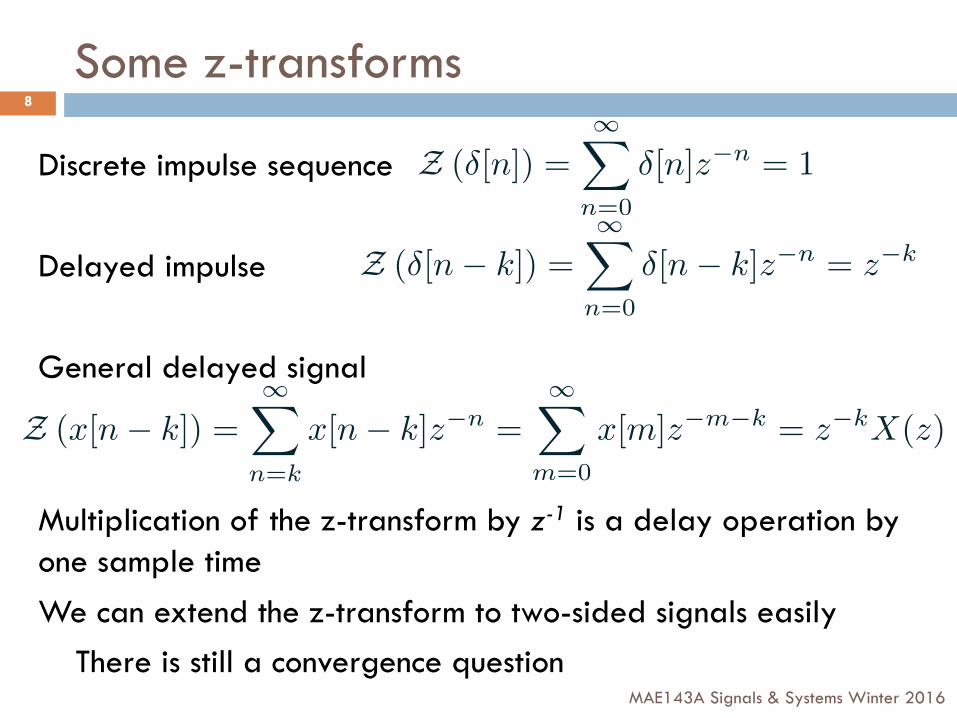
Z-transform of a discrete step


9

This uses the geometric series formula It converges if

We can extend this to a geometric series

This converges if

Z (1[n]) =1X

n=0

1z�n = 1 + z�1 + z�2 + · · · = 1

1� z�1=

z

z � 1

x[n] = a

n1[n]

Z(an1[n]) =1X

k=0

anz�n =1

1� az�1=

z

z � a

|z| > 1

|z| > |a|

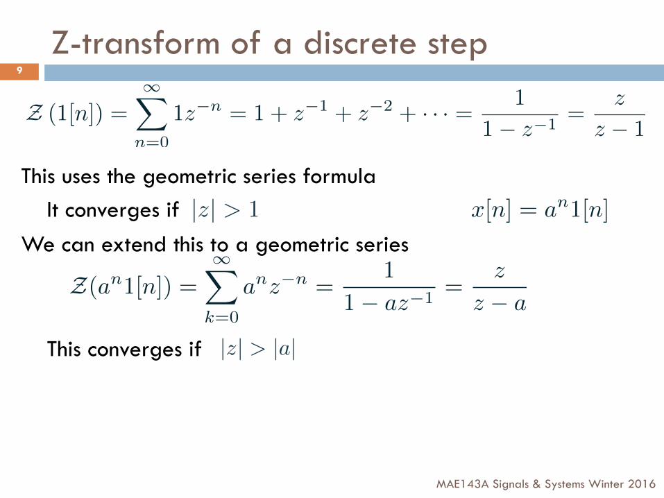
Z-transform and convolution


10

Z(x[n] ⇤ v[n]) =1X

n=0

1X

k=0

x[k]v[n� k]z�n

=1X

n=0

1X

k=0

x[k]z�kv[n� k]z�(n�k)

=1X

k=0

x[k]z�k1X

m=�k

v[m]z�m

=1X

k=0

x[k]z�k1X

m=0

v[m]z�m = X(z)V (z)

Z(x[n] ⇤ v[n]) = X(z)V (z)

Z-transforms


11

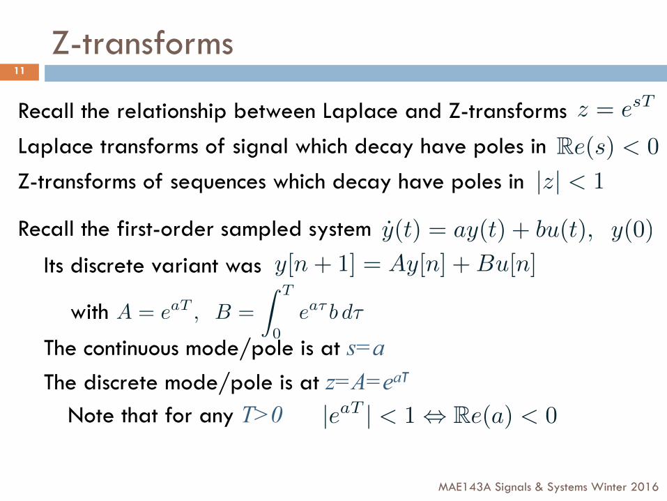
Recall the relationship between Laplace and Z-transforms Laplace transforms of signal which decay have poles in Z-transforms of sequences which decay have poles in

Recall the first-order sampled system

Its discrete variant was

with

The continuous mode/pole is at s=a The discrete mode/pole is at z=A=eaT

Note that for any T>0

z = esT

Re(s) < 0

|z| < 1

y(t) = ay(t) + bu(t), y(0)

A = eaT , B =

Z T

0ea� b d�

y[n+ 1] = Ay[n] +Bu[n]

|eaT | < 1 , Re(a) < 0

Z-transforms and delays


12

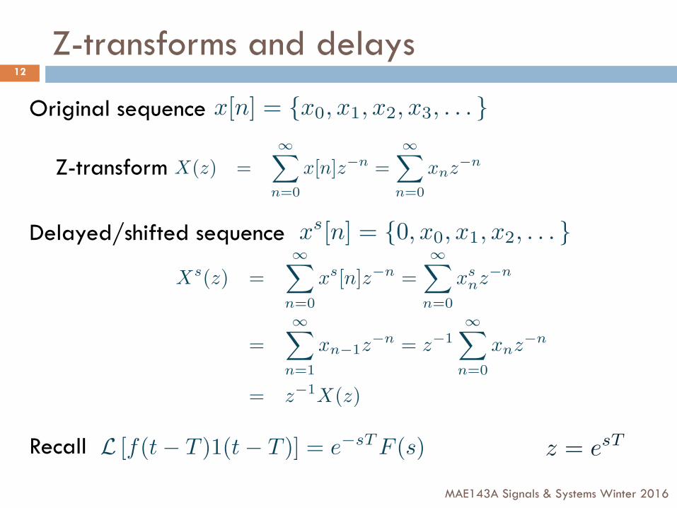
Original sequence

Z-transform

Delayed/shifted sequence

Recall

x[n] = {x0, x1, x2, x3, . . . }

x

s[n] = {0, x0, x1, x2, . . . }

X

s(z) =1X

n=0

x

s[n]z�n =1X

n=0

x

snz

�n

=1X

n=1

xn�1z�n = z

�11X

n=0

xnz

�n

= z

�1X(z)

X(z) =1X

n=0

x[n]z�n =1X

n=0

xnz

�n

L [f(t� T )1(t� T )] = e�sT F (s) z = esT

Discrete system transfer functions


13

Example ODE

Solve by recursion with initial conditions Let’s take the z-transform

Denote the solution z-t by and the input z-t by

A discrete transfer function The initial conditions get mixed in at recursion

y[n] + 0.1y[n� 1]� 0.72y[n� 2] = 0.1u[n� 1] + 0.9u[n� 2]

y[n] = �0.1y[n� 1] + 0.72y[n� 2] + 0.1u[n� 1] + 0.9u[n� 2]

U(z)Y (z)

1X

n=0

y[n]z�n = �0.11X

n=0

y[n� 1]z�n + 0.721X

n=0

y[n� 2]z�n + 0.11X

n=0

u[n� 1]z�n + 0.91X

n=0

u[n� 2]z�n

Y (z) = �0.1z�1Y (z) + 0.72z�2Y (z) + 0.1z�1U(z) + 0.9z�2U(z)Y (z) + 0.1z�1Y (z)� 0.72z�2Y (z) = 0.1z�1U(z) + 0.9z�2U(z)

Y (z) =0.1z�1 + 0.9z�2

1 + 0.1z�1 � 0.72z�2U(z)

MAE143a Signals & Systems Winter 2005 109

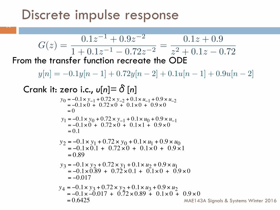
Discrete impulse response - by hand

Impulse response: zero i.c.s, un=!n

!

yn + .1yn"1 " 0.72yn"2 = .1un"1 + .9un"2

!

y0 = "0.1# y"1 + 0.72 # y"2 + 0.1# u"1 + 0.9 # u"2= "0.1# 0 + 0.72 # 0 + 0.1# 0 + 0.9 # 0= 0

!

y1 = "0.1# y0 + 0.72 # y"1 + 0.1# u0 + 0.9 # u"1= "0.1# 0 + 0.72 # 0 + 0.1#1 + 0.9 # 0= 0.1

!

y2 = "0.1# y1 + 0.72 # y0 + 0.1# u1 + 0.9 # u0= "0.1# 0.1 + 0.72 # 0 + 0.1# 0 + 0.9 #1= 0.89

!

y3 = "0.1# y2 + 0.72 # y1 + 0.1# u2 + 0.9 # u1= "0.1# 0.89 + 0.72 # 0.1 + 0.1# 0 + 0.9 # 0= "0.017

!

y4 = "0.1# y3 + 0.72 # y2 + 0.1# u3 + 0.9 # u2= "0.1#"0.017 + 0.72 # 0.89 + 0.1# 0 + 0.9 # 0= 0.6425

Discrete impulse response


14

From the transfer function recreate the ODE

Crank it: zero i.c., u[n]=δ[n]

G(z) =0.1z�1 + 0.9z�2

1 + 0.1z�1 � 0.72z�2=

0.1z + 0.9

z2 + 0.1z � 0.72

y[n] = �0.1y[n� 1] + 0.72y[n� 2] + 0.1u[n� 1] + 0.9u[n� 2]

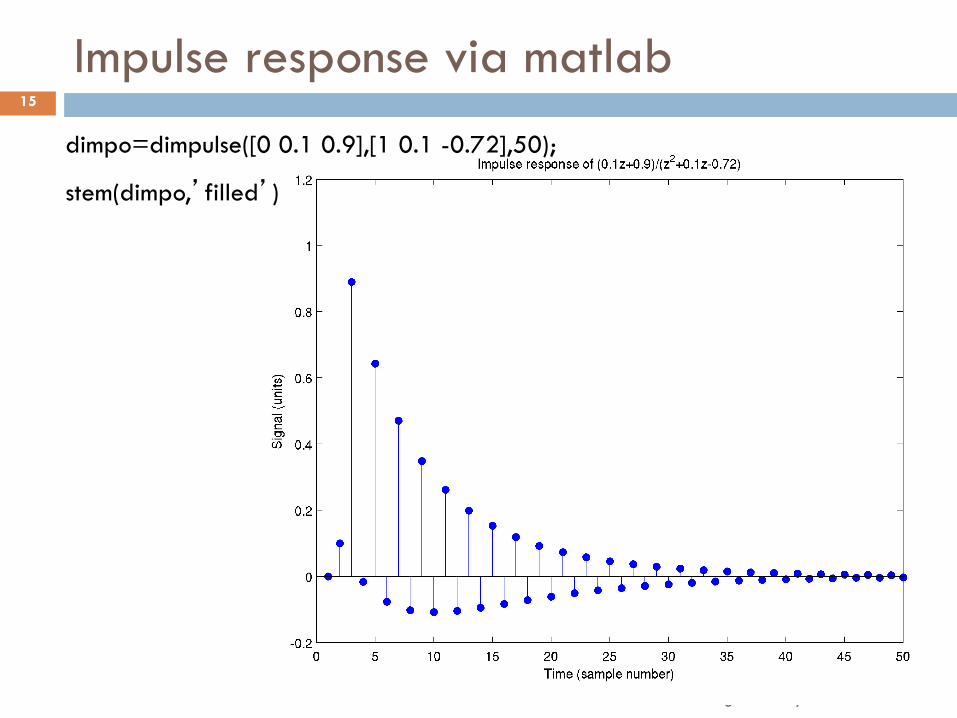
Impulse response via matlab


15

dimpo=dimpulse([0 0.1 0.9],[1 0.1 -0.72],50);

stem(dimpo,’filled’)

Impulse response via partial fractions


16

Same as for Laplace … and just as much fun

Note that the stable poles yield exponentially decaying terms

These modes are very fast – near z=-1 Rapid changes in the response

Y (z) = G(z)U(z) =0.1z�1 + 0.9z�2

1 + 0.1z�1 � 0.72z�2⇥ 1

=0.1z + 0.9

z2 + 0.1z � 0.72

=98/170z � 0.8

� 81/170z + 0.9

=98170

⇥ z�1

1� 0.8z�1� 81

170⇥ z�1

1 + 0.9z�1

=98170

z�1 ⇥ 11� 0.8z�1

� 81170

z�1 ⇥ 11 + 0.9z�1

=98170

z�1�1 + 0.8z�1 + 0.64z�2 + 0.512z�3 + . . .

�

� 81170

z�1�1� 0.9z�1 + 0.81z�2 � 0.729z�3 + . . .

�

= 0 + 0.1z�1 + 0.89z�2 � 0.017z�3 + 0.6425z�4 � . . .

= Z [{0, 0.1, 0.89,�0.017, 0.6425, . . . }]

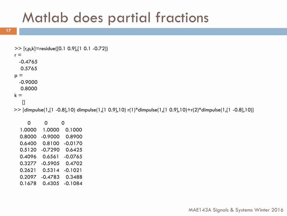
Matlab does partial fractions


17

>> [dimpulse(1,[1 -0.8],10) dimpulse(1,[1 0.9],10) r(1)*dimpulse(1,[1 0.9],10)+r(2)*dimpulse(1,[1 -0.8],10)] 0 0 0 1.0000 1.0000 0.1000 0.8000 -0.9000 0.8900 0.6400 0.8100 -0.0170 0.5120 -0.7290 0.6425 0.4096 0.6561 -0.0765 0.3277 -0.5905 0.4702 0.2621 0.5314 -0.1021 0.2097 -0.4783 0.3488 0.1678 0.4305 -0.1084

>> [r,p,k]=residue([0.1 0.9],[1 0.1 -0.72]) r = -0.4765 0.5765 p = -0.9000 0.8000 k = []

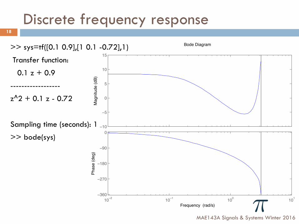
Discrete frequency response


18

>> sys=tf([0.1 0.9],[1 0.1 -0.72],1)

Transfer function:

0.1 z + 0.9

------------------

z^2 + 0.1 z - 0.72

Sampling time (seconds): 1

>> bode(sys)

−10

−5

0

5

10

15

Mag

nitu

de (d

B)

10−2 10−1 100 101−360

−270

−180

−90

0

Phas

e (d

eg)

Bode Diagram

Frequency (rad/s) ⇡

Summary of discrete time

Continuous-time Signals: functions Systems: ODEs, impulse response, state space Laplace transforms:

poles stability in Re[s]<0

Fourier transforms: Frequency content Frequency response Frequency axis

Convolution

Discrete-time Signals: sequences Systems: ODEs, impulse response, state space Z transforms:

Poles stability in |z|<1

Discrete Fourier transforms: Frequency content Frequency response Frequency axis

Convolution via FFT

19


s = j! z = ej!

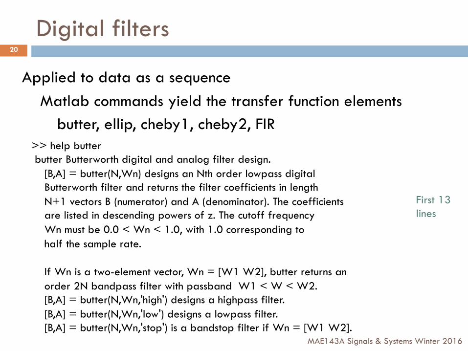
Digital filters


20

Applied to data as a sequence Matlab commands yield the transfer function elements

butter, ellip, cheby1, cheby2, FIR >> help butter butter Butterworth digital and analog filter design. [B,A] = butter(N,Wn) designs an Nth order lowpass digital Butterworth filter and returns the filter coefficients in length N+1 vectors B (numerator) and A (denominator). The coefficients are listed in descending powers of z. The cutoff frequency Wn must be 0.0 < Wn < 1.0, with 1.0 corresponding to half the sample rate. If Wn is a two-element vector, Wn = [W1 W2], butter returns an order 2N bandpass filter with passband W1 < W < W2. [B,A] = butter(N,Wn,'high') designs a highpass filter. [B,A] = butter(N,Wn,'low') designs a lowpass filter. [B,A] = butter(N,Wn,'stop') is a bandstop filter if Wn = [W1 W2].

First 13 lines

Documents

Discrete-time first-order systemsnumbat.ucsd.edu/~bob/signals2016Winter/Signals_&_Systems_2016... · Discrete-time first-order systems 1 Start with the continuous-time system Zero-order