Embed Size (px)
Citation preview

DISCRETE EXTERIOR CALCULUS
MATHIEU DESBRUN, ANIL N. HIRANI, MELVIN LEOK, AND JERROLD E. MARSDEN
Abstract. We present a theory and applications of discrete exterior calculus on simplicial complexes of
arbitrary finite dimension. This can be thought of as calculus on a discrete space. Our theory includes not
only discrete differential forms but also discrete vector fields and the operators acting on these objects. Thisallows us to address the various interactions between forms and vector fields (such as Lie derivatives) which
are important in applications. Previous attempts at discrete exterior calculus have addressed only differential
forms. We also introduce the notion of a circumcentric dual of a simplicial complex. The importance of dualcomplexes in this field has been well understood, but previous researchers have used barycentric subdivision
or barycentric duals. We show that the use of circumcentric duals is crucial in arriving at a theory of discrete
exterior calculus that admits both vector fields and forms.
Contents
1. Introduction 12. History and Previous Work 43. Primal Simplicial Complex and Dual Cell Complex 44. Local and Global Embeddings 105. Differential Forms and Exterior Derivative 126. Hodge Star and Codifferential 147. Maps between 1-Forms and Vector Fields 158. Wedge Product 179. Divergence and Laplace–Beltrami 2210. Contraction and Lie Derivative 2411. Discrete Poincare Lemma 2712. Discrete Variational Mechanics and DEC 3713. Extensions to Dynamic Problems 4413.1. Groupoid Interpretation of Discrete Variational Mechanics 4413.2. Discrete Diffeomorphisms and Discrete Flows 4513.3. Push-Forward and Pull-Back of Discrete Vector Fields and Discrete Forms 4714. Remeshing Cochains and Multigrid Extensions 4915. Conclusions and Future Work 50References 51
1. Introduction
This work presents a theory of discrete exterior calculus (DEC) motivated by potential applicationsin computational methods for field theories such as elasticity, fluids, and electromagnetism. In addition, itprovides much needed mathematical machinery to enable a systematic development of numerical schemesthat mirror the approach of geometric mechanics.
1
2 MATHIEU DESBRUN, ANIL N. HIRANI, MELVIN LEOK, AND JERROLD E. MARSDEN
This theory has a long history that we shall outline below in §2, but we aim at a comprehensive, systematic,as well as useful, treatment. Many previous works, as we shall review, are incomplete both in terms of theobjects that they treat as well as the types of meshes that they allow.
Our vision of this theory is that it should proceed ab initio as a discrete theory that parallels the continuousone. General views of the subject area of DEC are common in the literature (see, for instance, Mattiussi[2000]), but they usually stress the process of discretizing a continuous theory and the overall approach istied to this goal. However, if one takes the point of view that the discrete theory can, and indeed should,stand in its own right, then the range of application areas naturally is enriched and increases.
Convergence and consistency considerations alone are inadequate to discriminate between the variouschoices of discretization available to the numerical analyst, and only by requiring, when appropriate, thatthe discretization exhibits discrete analogues of continuous properties of interest can we begin to address thequestion of what makes a discrete theory a canonical discretization of a continuous one.
Applications to Variational Problems. One of the major application areas we envision is to variationalproblems, be they in mechanics or optimal control. One of the key ingredients in this direction that weimagine will play a key role in the future is that of AVI’s (asynchronous variational integrators) designed forthe numerical integration of mechanical systems, as in Lew et al. [2003]. These are integration algorithmsthat respect some of the key features of the continuous theory, such as their multi-symplectic nature andexact conservation laws. They do so by discretizing the underlying variational principles of mechanics ratherthan discretizing the equations. It is well-known (see the reference just mentioned for some of the literature)that variational problems come equipped with a rich exterior calculus structure and so on the discrete level,such structures will be enhanced by the availability of a discrete exterior calculus. One of the objectives ofthis chapter is to fill this gap.
Structured Constraints. There are many constraints in numerical algorithms that naturally involvedifferential forms, such as the divergence constraint for incompressibility of fluids, as well as the fact thatdifferential forms are naturally the fields in electromagnetism, and some of Maxwell’s equations are expressedin terms of the divergence and curl operations on these fields. Preserving, as in the mimetic differencingliterature, such features directly on the discrete level is another one of the goals, overlapping with our goalsfor variational problems.
Lattice Theories. Periodic crystalline lattices are of important practical interest in material science, and theanisotropic nature of the material properties arises from the geometry and connectivity of the intermolecularbonds in the lattice. It is natural to model these lattices as inherently discrete objects, and an understandingof discrete curvature that arises from DEC is particularly relevant, since part of the potential energy arisesfrom stretched bonds that can be associated with discrete curvature in the underlying relaxed configuration ofthe lattice. In particular, this could yield a more detailed geometric understanding of what happens at grainboundaries. Lattice defects can also be associated with discrete curvature when appropriately interpreted.The introduction of a discrete notion of curvature will lay the foundations for a better understanding of therole of geometry in the material properties of solids.
Some of the Key Theoretical Accomplishments. Our development of discrete exterior calculus in-cludes discrete differential forms, the Hodge star operator, the wedge product, the exterior derivative, aswell as contraction and the Lie derivative. For example, this approach leads to the proper definition of

DISCRETE EXTERIOR CALCULUS 3
discrete divergence and curl operators and has already resulted in applications like a discrete Hodge typedecomposition of 3D vector fields on irregular grids—see Tong et al. [2003].
Context. We present the theory and some applications of DEC in the context of simplicial complexes ofarbitrary finite dimension.
Methodology. We believe that the correct way to proceed with this program is to develop, as we havealready stressed, ab initio, a calculus on discrete manifolds which parallels the calculus on smooth manifoldsof arbitrary finite dimension. Chapters 6 and 7 of Abraham et al. [1988] are a good source for the conceptsand definitions in the smooth case. However we have tried to make this chapter as self-contained as possible.Indeed, one advantage of developing a calculus on discrete manifolds, as we do here, is pedagogical. Byusing concrete examples of discrete two- and three-dimensional spaces one can explain most of calculus onmanifolds at least formally as we will do using the examples in this chapter. The machinery of Riemannianmanifolds and general manifold theory from the smooth case is, strictly speaking, not required in the discreteworld. The technical terms that are used in this introduction will be defined in subsequent sections, butthey should be already familiar to someone who knows the usual exterior calculus on smooth manifolds.
The Objects in DEC. To develop a discrete theory, one must define discrete differential forms along withvector fields and operators involving these. Once discrete forms and vector fields are defined, a calculuscan be developed by defining the discrete exterior derivative (d), codifferential (δ) and Hodge star (∗) foroperating on forms, discrete wedge product (∧) for combining forms, discrete flat ([) and sharp (]) operatorsfor going between vector fields and 1-forms and discrete contraction operator (iX) for combining forms andvector fields. Once these are done, one can then define other useful operators. For example, a discrete Liederivative (£X) can be defined by requiring that the Cartan magic (or homotopy) formula hold. A discretedivergence in any dimension can be defined. A discrete Laplace–deRham operator (∆) can be defined usingthe usual definition of dδ+δd. When applied to functions, this is the same as the discrete Laplace–Beltramioperator (∇2), which is the defined as div curl. We define all these operators in this chapter.
The discrete manifolds we work with are simplicial complexes. We will recall the standard formal def-initions in §3 but familiar examples of simplicial complexes are meshes of triangles embedded in R3 andmeshes made up of tetrahedra occupying a portion of R3. We will assume that the angles and lengths onsuch discrete manifolds are computed in the embedding space RN using the standard metric of that space.In other words, in this chapter we do not address the issue of how to discretize a given smooth Riemannianmanifold, and how to embed it in RN , since there may be many ways to do this. For example, SO(3) canbe embedded in R9 with a constraint, or as the unit quaternions in R4. Another potentially important con-sideration in discretizing the manifold is that the topology of the simplicial complex should be the same asthe manifold to be discretized. This can be verified using the methods of computational homology (see, forexample, Kaczynski et al. [2004]), or discrete Morse theory (see, for example, Forman [2002], Wood [2003]).For the purposes of discrete exterior calculus, only local metric information is required, and we will commenttowards the end of §3 how to address the issue of embedding in a local fashion, as well as the criterion for agood global embedding.
Our development in this chapter is for the most part formal in that we choose appropriate geometricdefinitions of the various objects and quantities involved. For the most part, we do not prove that thesedefinitions converge to the smooth counterparts. The definitions are chosen so as to make some importanttheorems like the generalized Stokes’ theorem true by definition. Moreover, in the cases where previousresults are available, we have checked that the operators we obtain match the ones obtained by other means,such as variational derivations.

4 MATHIEU DESBRUN, ANIL N. HIRANI, MELVIN LEOK, AND JERROLD E. MARSDEN
2. History and Previous Work
The use of simplicial chains and cochains as the basic building blocks for a discrete exterior calculushas appeared in several papers. See, for instance, Sen et al. [2000], Adams [1996], Bossavit [2002c], andreferences therein. These authors view forms as linearly interpolated versions of smooth differential forms, aviewpoint originating from Whitney [1957], who introduced the Whitney and deRham maps that establishan isomorphism between simplicial cochains and Lipschitz differential forms.
We will, however, view discrete forms as real-valued linear functions on the space of chains. These areinherently discrete objects that can be paired with chains of oriented simplices, or their geometric duals,by the bilinear pairing of evaluation. In the next chapter, where we consider applications involving thecurvature of a discrete space, we will relax the condition that discrete forms are real-valued, and considergroup-valued forms.
Intuitively, this natural pairing of evaluation can be thought of as integration of the discrete form overthe chain. This difference from the work of Sen et al. [2000] and Adams [1996] is apparent in the definitionsof operations like the wedge product as well.
There is also much interest in a discrete exterior calculus in the computational electromagnetism commu-nity, as represented by Bossavit [2001, 2002a,b,c], Gross and Kotiuga [2001], Hiptmair [1999, 2001a,b, 2002],Mattiussi [1997, 2000], Nicolaides and Wang [1998], Teixeira [2001], and Tonti [2002].
Many of the authors cited above, for example, Bossavit [2002c], Sen et al. [2000], and Hiptmair [2002], alsointroduce the notions of dual complexes in order to construct the Hodge star operator. With the exceptionof Hiptmair, they use barycentric duals. This works if one develops a theory of discrete forms and does notintroduce discrete vector fields. We show later that to introduce discrete vector fields into the theory thenotion of circumcentric duals seems to be important.
Other authors, such as Moritz [2000], Moritz and Schwalm [2001], Schwalm et al. [1999], have incorporatedvector fields into the cochain based approach to exterior calculus by identifying vector fields with cochains,and having them supported on the same mesh. This is ultimately an unsatisfactory approach, since dualmeshes are essential as a means of encoding physically relevant phenomena such as fluxes across boundaries.
The use of primal and dual meshes arises most often as staggered meshes in finite volume and finitedifference methods. In fluid computations, for example, the density is often a cell-centered quantity, whichcan either be represented as a primal object by being associated with the 3-cell, or as a dual object associatedwith the 0-cell at the center of the 3-cell. Similarly, the flux across boundaries can be associated with the2-cells that make up the boundary, or the 1-cell which is normal to the boundary.
Another approach to a discrete exterior calculus is presented in Dezin [1995]. He defines a one-dimensionaldiscretization of the real line in much the same way we would. However, to generalize to higher dimensionshe introduces a tensor product of this space. This results in logically rectangular meshes. Our calculus,however, is defined over simplicial meshes. A further difference is that like other authors in this field, Dezin[1995] does not introduce vector fields into his theory.
A related effort for three-dimensional domains with logically rectangular meshes is that of Mansfieldand Hydon [2001], who established a variational complex for difference equations by constructing a discretehomotopy operator. We construct an analogous homotopy operator for simplicial meshes in proving thediscrete Poincare lemma.
3. Primal Simplicial Complex and Dual Cell Complex
In constructing the discretization of a continuous problem in the context of our formulation of discreteexterior calculus, we first discretize the manifold of interest as a simplicial complex. While this is typicallyin the form of a simplicial complex that is embedded into Euclidean space, it is only necessary to have anabstract simplicial complex, along with a local metric defined on adjacent vertices. This abstract setting willbe addressed further toward the end of this section.

DISCRETE EXTERIOR CALCULUS 5
We will now recall some basic definitions of simplices and simplicial complexes, which are standard fromsimplicial algebraic topology. A more extensive treatment can be found in Munkres [1984].
Definition 3.1. A k-simplex is the convex span of k + 1 geometrically independent points,
σk = [v0, v1, . . . , vk] =
k∑
i=0
αivi
∣∣∣∣∣αi ≥ 0,n∑
i=0
αi = 1
.
The points v0, . . . , vk are called the vertices of the simplex, and the number k is called the dimension ofthe simplex. Any simplex spanned by a (proper) subset of v0, . . . , vk is called a (proper) face of σk. Ifσl is a proper face of σk, we denote this by σl ≺ σk.
Example 3.1. Consider 3 non-collinear points v0, v1 and v2 in R3. Then, these three points individuallyare examples of 0-simplices, to which an orientation is assigned through the choice of a sign. Examples of1-simplices are the oriented line segments [v0, v1], [v1, v2] and [v0, v2]. By writing the vertices in that orderwe have given orientations to these 1-simplices, i.e., [v0, v1] is oriented from v0 to v1. The triangle [v0, v1, v2]is a 2-simplex oriented in counterclockwise direction. Note that the orientation of [v0, v2] does not agree withthat of the triangle.
Definition 3.2. A simplicial complex K in RN is a collection of simplices in RN , such that,(1) Every face of a simplex of K is in K.(2) The intersection of any two simplices of K is a face of each of them.
Definition 3.3. A simplicial triangulation of a polytope |K| is a simplicial complex K such that theunion of the simplices of K recovers the polytope |K|.
Definition 3.4. If L is a subcollection of K that contains all faces of its elements, then L is a simplicialcomplex in its own right, and it is called a subcomplex of K. One subcomplex of K is the collection of allsimplices of K of dimension at most k, which is called the k-skeleton of K, and is denoted K(k).
Circumcentric Subdivision. We will also use the notion of a circumcentric dual or Voronoi mesh of thegiven primal mesh. We will point to the importance of this choice later on in §7 and 9. We call the Voronoidual a circumcentric dual since the dual of a simplex is its circumcenter (equidistant from all vertices of thesimplex).
Definition 3.5. The circumcenter of a k-simplex σk is given by the center of the k-circumsphere, wherethe k-circumsphere is the unique k-sphere that has all k + 1 vertices of σk on its surface. Equivalently,the circumcenter is the unique point in the k-dimensional affine space that contains the k-simplex that isequidistant from all the k + 1 nodes of the simplex. We will denote the circumcenter of a simplex σk byc(σk).
The circumcenter of a simplex σk can be obtained by taking the intersection of the normals to the (k−1)-dimensional faces of the simplex, where the normals are emanating from the circumcenter of the face. Thisallows us to recursively compute the circumcenter.
If we are given the nodes which describe the primal mesh, we can construct a simplicial triangulation byusing the Delaunay triangulation, since this ensures that the circumcenter of a simplex is always a pointwithin the simplex. Otherwise we assume that a nice mesh has been given to us, i.e., it is such that thecircumcenters lie within the simplices. While this is not be essential for our theory it makes some proofssimpler. For some computations the Delaunay triangulation is desirable in that it reduces the maximumaspect ratio of the mesh, which is a factor in determining the rate at which the corresponding numericalscheme converges. But in practice there are many problems for which Delaunay triangulations are a badidea. See, for example, Schewchuck [2002]. We will address such computational issues in a separate work.

6 MATHIEU DESBRUN, ANIL N. HIRANI, MELVIN LEOK, AND JERROLD E. MARSDEN
Definition 3.6. The circumcentric subdivision of a simplicial complex is given by the collection of allsimplices of the form
[c(σ0), . . . , c(σk)],where σ0 ≺ σ1 ≺ . . . ≺ σk, or equivalently, that σi is a proper face of σj for all i < j.
Circumcentric Dual. We construct a circumcentric dual to a k-simplex using the circumcentric dualityoperator, which is introduced below.
Definition 3.7. The circumcentric duality operator is given by
?(σk)
=∑
σk≺σk+1≺...≺σn
εσk,...,σn
[c(σk), c(σk+1), . . . , c(σn)
],
where the εσk,...,σn coefficient ensures that the orientation of[c(σk), c(σk+1), . . . , c(σn)
]is consistent with
the orientation of the primal simplex, and the ambient volume-form.Orienting σk is equivalent to choosing a ordered basis, which we shall denote by dx1∧ . . .∧dxk. Similarly,[
c(σk), c(σk+1), . . . , c(σn)]
has an orientation denoted by dxk+1 ∧ . . .∧ dxn. If the orientation correspondingto dx1 ∧ . . . ∧ dxn is consistent with the volume-form on the manifold, then εσk,...,σn = 1, otherwise it takesthe value −1.
We immediately see from the construction of the circumcentric duality operator that the dual elementscan be realized as a submesh of the first circumcentric subdivision, since it consists of elements of the form[c(σ0), . . . , c(σk)], which are, by definition, part of the first circumcentric subdivision.
Example 3.2. The circumcentric duality operator maps a 0-simplex into the convex hull generated by thecircumcenters of n-simplices that contain the 0-simplex,
?(σ0) =∑
ασnc (σn)∣∣∣ασn ≥ 0,
∑ασn = 1, σ0 ≺ σn
,
and the circumcentric duality operator maps a n−simplex into the circumcenter of the n−simplex,
?(σn) = c(σn).
This is more clearly illustrated in Figure 1, where the primal and dual elements are color coded to representthe dual relationship between the elements in the primal and dual mesh.
(a) Primal (b) Dual (c) First subdivision
Figure 1: Primal, and dual meshes, as chains in the first circumcentric subdivision.
The choice of a circumcentric dual is significant, since it allows us to recover geometrically importantobjects such as normals to (n− 1)-dimensional faces, which are obtained by taking their circumcentric dual,
DISCRETE EXTERIOR CALCULUS 7
whereas, if we were to use a barycentric dual, the dual to a (n− 1)-dimensional face would not be normal toit.
Orientation of the Dual Cell. Notice that given an oriented simplex σk, which is represented by[v0, . . . , vk], the orientation is equivalently represented by (v1 − v0) ∧ (v2 − v1) ∧ . . . ∧ (vk − vk−1), which wedenote by,
[v0, . . . , vk] ∼ (v1 − v0) ∧ (v2 − v1) ∧ . . . ∧ (vk − vk−1),which is an equivalence at the level of orientation. It would be nice to express our criterion for determiningthe orientation of the dual cell in terms of the (k + 1)-vertex representation.
To determine the orientation of the (n − k)-simplex given by [c(σk), c(σk+1), . . . , c(σn)], or equivalently,dxk+1∧ . . .∧dxn, we consider the n-simplex given by [c(σ0), . . . , c(σn)], where σ0 ≺ . . . ≺ σk. This is relatedto the expression dx1 ∧ . . . ∧ dxn, up to a sign determined by the relative orientation of [c(σ0), . . . , c(σk)]and σk. Thus, we have that
dx1 ∧ . . . ∧ dxn ∼ sgn([c(σ0), . . . , c(σk)], σk)[c(σ0), . . . , c(σn)] .
Then, we need to check that dx1∧. . .∧dxn is consistent with the volume-form on the manifold, which is repre-sented by the orientation of σn. Thus, we have that the correct orientation for the [c(σk), c(σk+1), . . . , c(σn)]term is given by,
sgn([c(σ0), . . . , c(σk)], σk) · sgn([c(σ0), . . . , c(σn)], σn).These two representations of the choice of orientation for the dual cells are equivalent, but the combinatorialdefinition above might be preferable for the purposes of implementation.
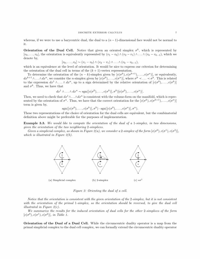
Example 3.3. We would like to compute the orientation of the dual of a 1-simplex, in two dimensions,given the orientation of the two neighboring 2-simplices.
Given a simplicial complex, as shown in Figure 2(a), we consider a 2-simplex of the form [c(σ0), c(σ1), c(σ2)],which is illustrated in Figure 2(b).
(a) Simplicial complex (b) 2-simplex (c) ?σ1
Figure 2: Orienting the dual of a cell.
Notice that the orientation is consistent with the given orientation of the 2-simplex, but it is not consistentwith the orientation of the primal 1-simplex, so the orientation should be reversed, to give the dual cellillustrated in Figure 2(c).
We summarize the results for the induced orientation of dual cells for the other 2-simplices of the form[c(σ0), c(σ1), c(σ2)], in Table 1.
Orientation of the Dual of a Dual Cell. While the circumcentric duality operator is a map from theprimal simplicial complex to the dual cell complex, we can formally extend the circumcentric duality operator

8 MATHIEU DESBRUN, ANIL N. HIRANI, MELVIN LEOK, AND JERROLD E. MARSDEN
Table 1. Determining the induced orientation of a dual cell.
[c(σ0), c(σ1), c(σ2)]
sgn([c(σ0), c(σ1)], σ1) − + + −
sgn([c(σ0), c(σ1), c(σ2)], σ2) + − + −
sgn([c(σ0), c(σ1)], σ1)· sgn([c(σ0), c(σ1), c(σ2)], σ2)·[c(σ1), c(σ2)]
to a map from the dual cell complex to the primal simplicial complex. However, we need to be slightly carefulabout the orientation of primal simplex we recover from applying the circumcentric duality operator twice.
We have that, ? ? (σk) = ±σk, where the sign is chosen to ensure the appropriate choice of orientation.If, as before, σk has an orientation represented by dx1 ∧ . . . ∧ dxk, and ?σk has an orientation representedby dxk+1 ∧ . . . ∧ dxn, then the orientation of ? ? (σk) is chosen so that dxk+1 ∧ . . . ∧ dxn ∧ dx1 ∧ . . . ∧ dxk isconsistent with the ambient volume-form. Since, by construction, ?(σk), dx1 ∧ . . . ∧ dxn has an orientationconsistent with the ambient volume-form, we need only compare dxk+1 ∧ . . . ∧ dxn ∧ dx1 ∧ . . . ∧ dxk withdx1∧ . . .∧dxn. Notice that it takes n−k transpositions to get the dx1 term in front of the dxk+1∧ . . .∧dxn
terms, and we need to do this k times for each term of dx1 ∧ . . . ∧ dxk, so it follows that the sign is simplygiven by (−1)k(n−k), or equivalently,
(3.1) ? ? (σk) = (−1)k(n−k)σk.
A similar relationship holds if we use a dual cell instead of the primal simplex σk.
Support Volume of a Primal Simplex and Its Dual Cell. We can think of a cochain as beingconstructed out of a basis consisting of cosimplices or cocells with value 1 on a single simplex or cell, and0 otherwise. The way to visualize this cosimplex is that it is associated with a differential form that hassupport on what we will refer to as the support volume associated with a given simplex or cell.
Definition 3.8. The support volume of a simplex σk is a n-volume given by the convex hull of the geometricunion of the simplex and its circumcentric dual. This is given by
Vσk = convexhull(σk, ?σk) ∩ |K|.The intersection with |K| is necessary to ensure that the support volume does not extend beyond the
polytope |K| which would otherwise occur if |K| is nonconvex.We extend the notion of a support volume to a dual cell ?σk by similarly defining
V?σk = convexhull(?σk, ? ? σk) ∩ |K| = Vσk .

DISCRETE EXTERIOR CALCULUS 9
To clarify this definition, we will consider some examples of simplices, their dual cells, and their corre-sponding support volumes. For two-dimensional simplicial complexes, this is illustrated in Table 2.
Table 2. Primal simplices, dual cells, and support volumes in two dimensions.
Primal Simplex Dual Cell Support Volume
σ0, 0-simplex ?σ0, 2-cell Vσ0 = V?σ0
σ1, 1-simplex ?σ1, 1-cell Vσ1 = V?σ1
σ2, 2-simplex ?σ2, 0-cell Vσ2 = V?σ2
The support volume has the nice property that at each dimension, it partitions the polytope |K| intodistinct non-intersecting regions associated with each individual k-simplex. For any two distinct k-simplices,the intersection of their corresponding support volumes have measure zero, and the union of the supportvolumes of all k-simplices recovers the original polytope |K|.
Notice, from our construction, that the support volume of a simplex and its dual cell are the same, whichsuggests that there is an identification between cochains on k-simplices and cochains on (n− k)-cells. Thisis indeed the case, and is a concept associated with the Hodge star for differential forms.
Examples of simplices, their dual cells, and the corresponding support volumes in three dimensions aregiven in Table 3.
In our subsequent discussion, we will assume that we are given a simplicial complex K of dimension n inRN . Thus, the highest-dimensional simplex in the complex is of dimension n and each 0-simplex (vertex) isin RN . One can obtain this, for example, by starting from 0-simplices, i.e., vertices, and then constructing aDelaunay triangulation, using the vertices as sites. Often, our examples will be for two-dimensional discretesurfaces in R3 made up of triangles (here n = 2 and N = 3) or three-dimensional manifolds made oftetrahedra, possibly embedded in a higher-dimensional space.
Cell Complexes. The circumcentric dual of a primal simplicial complex is an example of a cell complex.The definition of a cell complex follows.
Definition 3.9. A cell complex ?K in RN is a collection of cells in RN such that,(1) There is a partial ordering of cells in ?K, σk ≺ σl, which is read as σk is a face of σl.(2) The intersection of any two cells in ?K, is either a face of each of them, or it is empty.(3) The boundary of a cell is expressible as a sum of its proper faces.

10 MATHIEU DESBRUN, ANIL N. HIRANI, MELVIN LEOK, AND JERROLD E. MARSDEN
Table 3. Primal simplices, dual cells, and support volumes in three dimensions.
Primal Simplex Dual Cell Support Volume
σ0, 0-simplex ?σ0, 3-cell Vσ0 = V?σ0
σ1, 1-simplex ?σ1, 2-cell Vσ1 = V?σ1
σ2, 2-simplex ?σ2, 1-cell Vσ2 = V?σ2
σ3, 3-simplex ?σ3, 0-cell Vσ3 = V?σ3
We will see in the next section that the notion of boundary in the circumcentric dual has to be modifiedslightly from the geometric notion of a boundary in order for the circumcentric dual to be made into a cellcomplex.
4. Local and Global Embeddings
While it is computationally more convenient to have a global embedding of the simplicial complex into ahigher-dimensional ambient space to account for non-flat manifolds it suffices to have an abstract simplicialcomplex along with a local metric on vertices. The metric is local in the sense that distances between two

DISCRETE EXTERIOR CALCULUS 11
vertices are only defined if they are part of a common n-simplex in the abstract simplicial complex. Then,the local metric is a map d : (v0, v1) | v0, v1 ∈ K(0), [v0, v1] ≺ σn ∈ K → R.
The axioms for a local metric are as follows,Positive.: d(v0, v1) ≥ 0, and d(v0, v0) = 0, ∀[v0, v1] ≺ σn ∈ K.Strictly Positive.: If d(v0, v1) = 0, then v0 = v1, ∀[v0, v1] ≺ σn ∈ K.Symmetry.: d(v0, v1) = d(v1, v0), ∀[v0, v1] ≺ σn ∈ K.Triangle Inequality.: d(v0, v2) ≤ d(v0, v1) + d(v1, v2), ∀[v0, v1, v2] ≺ σn ∈ K.
This allows us to embed each n-simplex locally into Rn, and thereby compute all the necessary metricdependent quantities in our formulation. For example, the volume of a k-dual cell will be computed as thesum of the k-volumes of the dual cell restricted to each n-simplex in its local embedding into Rn.
This notion of local metrics and local embeddings is consistent with the point of view that exterior calculusis a local theory with operators that operate on objects in the tangent and cotangent space of a fixed point.The issue of comparing objects in different tangent spaces is addressed in the discrete theory of connectionson principal bundles in Leok et al. [2003].
This also provides us with a criterion for evaluating a global embedding. The embedding should be suchthat the metric of the ambient space RN restricted to the vertices of the complex, thought of as points in RN ,agrees with the local metric imposed on the abstract simplicial complex. A global embedding that satisfiesthis condition will produce the same numerical results in discrete exterior calculus as that obtained usingthe local embedding method.
It is essential that the metric condition we impose is local, since the notion of distances between points ina manifold which are far away is not a well-defined concept, nor is it particularly useful for embeddings. Asthe simple example below illustrates, there may not exist any global embeddings into Euclidean space thatsatisfies a metric constraint imposed for all possible pairs of vertices.
Example 4.1. Consider a circle, with the distance between two points given by the minimal arc length.Consider a discretization given by 4 equidistant points on the circle, labelled v0, . . . , v3, with the metricdistances as follows,
d(vi, vi+1) = 1, d(vi, vi+2) = 2,
where the indices are evaluated modulo 4, and this distance function is extended to a metric on all pairs ofvertices by symmetry. It is easy to verify that this distance function is indeed a metric on vertices.
0 '!&"%#$
1 '!&"%#$
2 '!&"%#$????
????
? 3 '!&"%#$
?????????
1
2
If we only use the local metric constraint, then we only require that adjacent vertices are separated by 1, andthe following is an embedding of the simplicial complex into R2,
1
1
????
????
????
?
1
1
?????????????

12 MATHIEU DESBRUN, ANIL N. HIRANI, MELVIN LEOK, AND JERROLD E. MARSDEN
If, however, we use the metric defined on all possible pairs of vertices, by considering v0, v1, v2, we have thatd(v0, v1) + d(v1, v2) = d(v0, v2). Since we are embedding these points into a Euclidean space, it follows thatv0, v1, v2 are collinear.
Similarly, by considering v0, v2, v3, we conclude that they are collinear as well, and that v1, v3 are coinci-dent, which contradicts d(v1, v3) = 2. Thus, we find that there does not exist a global embedding of the circleinto Euclidean space if we require that the embedding is consistent with the metric on vertices defined for allpossible pairs of vertices.
5. Differential Forms and Exterior Derivative
We will now define discrete differential forms. We will use some terms (which we will define) from algebraictopology, but it will become clear by looking at the examples that one can gain a clear and working notionof what a discrete form is without any algebraic topology. We start with a few definitions for which moredetails can be found on page 26 and 27 of Munkres [1984].
Definition 5.1. Let K be a simplicial complex. We denote the free abelian group generated by a basisconsisting of oriented k-simplices by Ck (K; Z) . This is the space of finite formal sums of the k-simplices,with coefficients in Z. Elements of Ck(K; Z) are called k-chains.
Example 5.1. Figure 3 shows examples of 1-chains and 2-chains.
12 1
3
2−chain1−chain
•
•
•
••
•
•
•
•
•
•
????
??? yyyyyyyyyy
cccccccc
\\\\\\\\\\\ ****
****1
&&NNNNNNNN
3::vvvv 2
77
777
5
II
Figure 3: Examples of chains.
We view discrete k-forms as maps from the space of k-chains to R. Recalling that the space of k-chainsis a group, we require that these maps be homomorphisms into the additive group R. Thus, discrete formsare what are called cochains in algebraic topology. We will define cochains below in the definition of formsbut for more context and more details readers can refer to any algebraic topology text, for example, page251 of Munkres [1984].
This point of view of forms as cochains is not new. The idea of defining forms as cochains appears, forexample, in the works of Adams [1996], Dezin [1995], Hiptmair [1999], and Sen et al. [2000]. Our point ofdeparture is that the other authors go on to develop a theory of discrete exterior calculus of forms only byintroducing interpolation of forms, which we will be able to avoid. The formal definition of discrete formsfollows.
Definition 5.2. A primal discrete k-form α is a homomorphism from the chain group Ck(K; Z) to theadditive group R. Thus, a discrete k-form is an element of Hom(Ck(K),R), the space of cochains. Thisspace becomes an abelian group if we add two homomorphisms by adding their values in R. The standardnotation for Hom(Ck(K),R) in algebraic topology is Ck(K; R). But we will often use the notation Ωk
d(K)for this space as a reminder that this is the space of discrete (hence the d subscript) k-forms on the simplicialcomplex K. Thus,
Ωkd(K) := Ck(K; R) = Hom(Ck(K),R) .

DISCRETE EXTERIOR CALCULUS 13
Note that, by the above definition, given a k-chain∑
i aicki (where ai ∈ Z) and a discrete k-form α, we
have that
α
(∑i
aicki
)=∑
i
aiα(cki ) ,
and for two discrete k-forms α, β ∈ Ωkd(K) and a k-chain c ∈ Ck(K; Z),
(α+ β)(c) = α(c) + β(c) .
In the usual exterior calculus on smooth manifolds integration of k-forms on a k-dimensional manifold isdefined in terms of the familiar integration in Rk. This is done roughly speaking by doing the integration inlocal coordinates, and showing that the value is independent of the choice of coordinates, due to the changeof variables theorem in Rk. For details on this, see the first few pages of Chapter 7 of Abraham et al. [1988].We will not try to introduce the notion of integration of discrete forms on a simplicial complex. Instead thefundamental quantity that we will work with is the natural bilinear pairing of cochains and chains, definedby evaluation. More formally, we have the following definition.
Definition 5.3. The natural pairing of a k-form α and a k-chain c is defined as the bilinear pairing
〈α, c〉 = α(c).
As mentioned above, in discrete exterior calculus, this natural pairing plays the role that integration offorms on chains plays in the usual exterior calculus on smooth manifolds. The two are related by a proceduredone at the time of discretization. Indeed, consider a simplicial triangulation K of a polyhedron in Rn, i.e.,consider a “flat” discrete manifold. If we are discretizing a continuous problem, we will have some smoothforms defined in the space |K| ⊂ Rn. Consider such a smooth k-form αk. In order to define the discreteform αk
d corresponding to αk, one would integrate αk on all the k-simplices in K. Then, the evaluation of αkd
on a k-simplex σk is defined by αkd(σk) :=
∫σk α
k. Thus, discretization is the only place where integrationplays a role in our discrete exterior calculus.
In the case of a non-flat manifold, the situation is somewhat complicated by the fact that the smoothmanifold, and the simplicial complex, as geometric sets embedded in the ambient space do not coincide. Asmooth differential form on the manifold can be discretized into the cochain representation by identifyingthe vertices of the simplicial complex with points on the manifold, and then using a local chart to identifyk-simplices with k-volumes on the manifold.
There is the possibility of k-volumes overlapping even when their corresponding k-simplices do not inter-sect, and this introduces a discretization error that scales like the mesh size. One can alternatively constructgeodesic boundary surfaces in an inductive fashion, which yields a partition of the manifold, but this can becomputationally prohibitive to compute.
Now we can define the discrete exterior derivative which we will call d, as in the usual exterior calculus.The discrete exterior derivative will be defined as the dual, with respect to the natural pairing defined above,of the boundary operator, which is defined below.
Definition 5.4. The boundary operator ∂k : Ck(K; Z) → Ck−1(K; Z) is a homomorphism defined by itsaction on a simplex σk = [v0, . . . , vk],
∂kσk = ∂k([v0, . . . , vk]) =
k∑i=0
(−1)i[v0, . . . , vi, . . . , vk] ,
where [v0, . . . , vi, . . . , vk] is the (k − 1)-simplex obtained by omitting the vertex vi. Note that ∂k ∂k+1 = 0.
Example 5.2. Given an oriented triangle [v0, v1, v2] the boundary, by the above definition, is the chain[v1, v2]− [v0, v2] + [v0, v1], which are the three boundary edges of the triangle.

14 MATHIEU DESBRUN, ANIL N. HIRANI, MELVIN LEOK, AND JERROLD E. MARSDEN
Definition 5.5. On a simplicial complex of dimension n, a chain complex is a collection of chain groupsand homomorphisms ∂k, such that,
0 // Cn(K)∂n // . . .
∂k+1// Ck(K)
∂k // . . . ∂1 // C0(K) // 0 ,
and ∂k ∂k+1 = 0.
Definition 5.6. The coboundary operator, δk : Ck(K) → CK+1(K), is defined by duality to the boundaryoperator, with respect to the natural bilinear pairing between discrete forms and chains. Specifically, for adiscrete form αk ∈ Ωk
d(K), and a chain ck+1 ∈ Ck+1(K; Z), we define δk by
(5.1)⟨δkαk, ck+1
⟩=⟨αk, ∂k+1ck+1
⟩.
That is to sayδk(αk) = αk ∂k+1 .
This definition of the coboundary operator induces the cochain complex,
0 Cn(K)oo . . .δn−1oo Ck(K)δk
oo . . .δk−1oo C0(K)δ0
oo 0oo ,
where it is easy to see that δk+1 δk = 0.
Definition 5.7. The discrete exterior derivative denoted by d : Ωkd(K) → Ωk+1
d (K) is defined to be thecoboundary operator δk.
Remark 5.1. With the above definition of the exterior derivative, d : Ωkd(K) → Ωk+1
d (K), and the rela-tionship between the natural pairing and integration, one can regard equation 5.1 as a discrete generalizedStokes’ theorem. Thus, given a k-chain c, and a discrete k-form α, the discrete Stokes’ theorem, which istrue by definition, states that
〈dα, c〉 = 〈α, ∂c〉 .Furthermore, it also follows immediately that dk+1dk = 0.
Dual Discrete Forms. Everything we have said above in terms of simplices and the simplicial complex Kcan be said in terms of the cells that are duals of simplices and elements of the dual complex ?K. One justhas to be a little more careful in the definition of the boundary operator, and the definition we constructbelow is well-defined on the dual cell complex. This gives us the notion of cochains of cells in the dualcomplex and these are the dual discrete forms.
Definition 5.8. The dual boundary operator, ∂k : Ck (?K; Z) → Ck−1 (?K; Z), is a homomorphism definedby its action on a dual cell σk = ?σn−k = ?[v0, . . . , vn−k],
∂σk = ∂ ? [v0, ..., vn−k]
=∑
σn−k+1σn−k
?σn−k+1 ,
where σn−k+1 is oriented so that it is consistent with the induced orientation on σn−k.
6. Hodge Star and Codifferential
In the exterior calculus for smooth manifolds, the Hodge star, denoted ∗, is an isomorphism between thespace of k-forms and (n−k)-forms. The Hodge star is useful in defining the adjoint of the exterior derivativeand this is adjoint is called the codifferential. The Hodge star, ∗ : Ωk(M) → Ωn−k(M), is in the smoothcase uniquely defined by the identity,
〈〈αk, βk〉〉v = αk ∧ ∗βk ,

DISCRETE EXTERIOR CALCULUS 15
where 〈〈 , 〉〉 is a metric on differential forms, and v is the volume-form. For a more in-depth discussion, see,for example, page 411 of Abraham et al. [1988].
The appearance of k and (n − k) in the definition of Hodge star may be taken to be a hint that primaland dual meshes will play some role in the definition of a discrete Hodge star, since the dual of a k-simplexis an (n− k)-cell. Indeed, this is the case.
Definition 6.1. The discrete Hodge Star is a map ∗ : Ωkd(K) → Ωn−k
d (?K), defined by its action onsimplices. For a k-simplex σk, and a discrete k-form αk,
1|σk|
〈αk, σk〉 =1
| ? σk|〈∗αk, ?σk〉.
The idea that the discrete Hodge star maps primal discrete forms to dual forms, and vice versa, is well-known. See, for example, Sen et al. [2000]. However, notice we now make use of the volume of these primaland dual meshes. But the definition we have given above does appear in the work of Hiptmair [2002].
The definition implies that the primal and dual averages must be equal. This idea has already beenintroduced, not in the context of exterior calculus, but in an attempt at defining discrete differential geometryoperators, see Meyer et al. [2002].
Remark 6.1. Although we have defined the discrete Hodge star above, we will show in Remark 12.1 of §12that if an appropriate discrete wedge product and metric on discrete k-forms is defined, then the expressionfor the discrete Hodge star operator follows from the smooth definition.
Lemma 6.1. For a k-form αk,∗ ∗ αk = (−1)k(n−k)αk .
Proof. The proof is a simple calculation using the property that for a simplex or a cell σk, ? ? (σk) =(−1)k(n−k)σk (Equation 3.1).
Definition 6.2. Given a simplicial or a dual cell complex K the discrete codifferential operator, δ :Ωk+1
d (K) → Ωkd(K), is defined by δ(Ω0
d(K)) = 0 and on discrete (k + 1)-forms to be
δβ = (−1)nk+1 ∗ d ∗ β .
With the discrete forms, Hodge star, d and δ defined so far, we already have enough to do an interestingcalculation involving the Laplace–Beltrami operator. But, we will show this calculation in §9 after we haveintroduced discrete divergence operator.
7. Maps between 1-Forms and Vector Fields
Just as discrete forms come in two flavors, primal and dual (being linear functionals on primal chainsor chains made up of dual cells), discrete vector fields also come in two flavors. Before formally definingprimal and dual discrete vector fields, consider the examples illustrated in Figure 4. The distinction lies inthe choice of basepoints, be they primal or dual vertices, to which we assign vectors.
Definition 7.1. Let K be a flat simplicial complex, that is, the dimension of K is the same as that of theembedding space. A primal discrete vector field X on a flat simplicial complex K is a map from thezero-dimensional primal subcomplex K(0) (i.e., the primal vertices) to RN . We will denote the space of suchvector fields by Xd(K). The value of such a vector field is piecewise constant on the dual n-cells of ?K.Thus, we could just as well have called such vector fields dual and defined them as functions on the n-cellsof ?K.
Definition 7.2. A dual discrete vector field X on a simplicial complex K is a map from the zero-dimensional dual subcomplex (?K)(0) (i.e, the circumcenters of the primal n simplices) to RN such that itsvalue on each dual vertex is tangential to the corresponding primal n-simplex. We will denote the space of

16 MATHIEU DESBRUN, ANIL N. HIRANI, MELVIN LEOK, AND JERROLD E. MARSDEN
(a) Primal vector field (b) Dual vector field
Figure 4: Discrete vector fields.
such vector fields by Xd(?K). The value of such a vector field is piecewise constant on the n-simplices ofK. Thus, we could just as well have called such vector fields primal and defined them as functions on then-simplices of K.
Remark 7.1. In this paper we have defined the primal vector fields only for flat meshes. We will addressthe issue of non-flat meshes in separate work.
As in the smooth exterior calculus, we want to define the flat ([) and sharp (]) operators that relate formsto vector fields. This allows one to write various vector calculus identities in terms of exterior calculus.
Definition 7.3. Given a simplicial complex K of dimension n, the discrete flat operator on a dualvector field, [ : Xd(?K) → Ωd(K), is defined by its evaluation on a primal 1 simplex σ1,
〈X[, σ1〉 =∑
σnσ1
| ? σ1 ∩ σn|| ? σ1|
X · ~σ1 ,
where X · ~σ1 is the usual dot product of vectors in RN , and ~σ1 stands for the vector corresponding to σ1,and with the same orientation. The sum is over all σn containing the edge σ1. The volume factors are indimension n.
Definition 7.4. Given a simplicial complex K of dimension n, the discrete sharp operator on a primal1-form, ] : Ωd(K) → Xd(?K), is defined by its evaluation on a given vertex v,
α](v) =∑
[v,σ0]
〈α, [v, σ0]〉∑
σn[v,σ0]
| ? v ∩ σn||σn|
n[v,σ0] ,
where the outer sum is over all 1-simplices containing the vertex v, and the inner sum is over all n-simplicescontaining the 1-simplex [v, σ0]. The volume factors are in dimension n, and the vector n[v,σ0] is the normalvector to the simplex [v, σ0], pointing into the n-simplex σn.
For a discussion of the proliferation of discrete sharp and flat operators that arise from considering theinterpolation of differential forms and vector fields, please see Hirani [2003].

DISCRETE EXTERIOR CALCULUS 17
8. Wedge Product
As in the smooth case, the wedge product we will construct is a way to build higher degree forms fromlower degree ones. For information about the smooth case, see the first few pages of Chapter 6 of Abrahamet al. [1988].
Definition 8.1. Given a primal discrete k-form αk ∈ Ωkd(K), and a primal discrete l-form βl ∈ Ωl
d(K), thediscrete primal-primal wedge product, ∧ : Ωk
d(K)× Ωld(K) → Ωk+l
d (K), defined by the evaluation on a(k + l)-simplex σk+l = [v0, . . . , vk+l] is given by
〈αk ∧ βl, σk+l〉 =1
(k + l)!
∑τ∈Sk+l+1
sign(τ)|σk+l ∩ ?vτ(k)|
|σk+l|α ^ β(τ(σk+l)) ,
where Sk+l+1 is the permutation group, and its elements are thought of as permutations of the numbers0, . . . , k + l + 1. The notation τ(σk+l) stands for the simplex [vτ(0), . . . , vτ(k+l)]. Finally, the notationα ^ β(τ(σk+l)) is borrowed from algebraic topology (see, for example, page 206 of Hatcher [2001]) and isdefined as
α ^ β(τ(σk+l)) := 〈α,[vτ(0), . . . , vτ(k)
]〉〈β,
[vτ(k), . . . , vτ(k+l)
]〉 .
Example 8.1. When we take the wedge product of two discrete 1-forms, we obtain terms in the sum thatare graphically represented in Figure 5.
Figure 5: Terms in the wedge product of two discrete 1-forms.
Definition 8.2. Given a dual discrete k-form αk ∈ Ωkd(?K), and a primal discrete l-form βl ∈ Ωl
d(?K), thediscrete dual-dual wedge product, ∧ : Ωk
d(?K) × Ωld(?K) → Ωk+l
d (?K), defined by the evaluation on a(k + l)-cell σk+l = ?σn−k−l, is given by
〈αk ∧ βl, σk+l〉 =〈αk ∧ βl, ?σn−k−l〉
=∑
σnσn−k−l
sign(σn−k−l, [vk+l, . . . , vn])∑
τ∈Sk+l
sign(τ)
· 〈αk, ?[vτ(0), . . . , vτ(l−1), vk+l, . . . , vn]〉〈βl, ?[vτ(l), . . . , vτ(k+l−1), vk+l, . . . , vn]〉
where σn = [v0, . . . , vn], and, without loss of generality, assumed that σn−k−l = ±[vk+l, . . . , vn].
Anti-Commutativity of the Wedge Product.
Lemma 8.1. The discrete wedge product, ∧ : Ck(K)× Cl(K) → Ck+l(K), is anti-commutative, i.e.,
αk ∧ βk = (−1)klβl ∧ αk .
Proof. We first rewrite the expression for the discrete wedge product using the following computation,∑τ∈Sk+l+1
sign(τ)|σk+l ∩ ?vτ(k)|〈αk, τ [v0, . . . , vk]〉βl, τ [vk, . . . , vk+l]〉

18 MATHIEU DESBRUN, ANIL N. HIRANI, MELVIN LEOK, AND JERROLD E. MARSDEN
=∑
τ∈Sk+l+1
(−1)k−1 sign(τ)|σk+l ∩ ?vτ(k)| 〈αk, τ [v1, . . . , v0, vk]〉〈βl, τ [vk, . . . , vk+l]〉
=∑
τ∈Sk+l+1
(−1)k−1 sign(τ)|σk+l ∩ ?vτρ(0)|〈αk, τρ[v1, . . . , vk, v0]〉〈βl, τρ[v0, vk+1, . . . , vk+l]〉
=∑
τ∈Sk+l+1
(−1)k−1(−1)k sign(τ)|σk+l ∩ ?vτρ(0)|〈αk, τρ[v0, . . . , vk]〉〈βl, τρ[v0, vk+1, . . . , vk+l]〉
=∑
τρ∈Sk+l+1ρ
(−1)k−1(−1)k(−1) sign(τ ρ)|σk+l ∩ ?vτρ(0)|
· 〈αk, τρ[v0, . . . , vk]〉〈βl, τρ[v0, vk+1, . . . , vk+l]〉
=∑
τ∈Sk+l+1
sign(τ)|σk+l ∩ ?vτ(0)|〈αk, τ [v0, . . . , vk]〉〈βl, τ [v0, vk+1, . . . , vk+l]〉 .
Here, we used the elementary fact, from permutation group theory, that a k + 1 cycle can be written asthe product of k transpositions, which accounts for the (−1)k factors. Also, ρ is a transposition of 0 and k.Then, the discrete wedge product can be rewritten as
〈αk ∧ βl, σk+l〉 =1
(k + l)!
∑τ∈Sk+l+1
sign(τ)|σk+l ∩ ?vτ(0)|
|σk+l|
· 〈αk, [vτ(0), . . . , vτ(k)]〉〈βl, [vτ(0),τ(k+1), . . . , vτ(k+l)]〉.
For ease of notation, we denote [v0, . . . , vk] by σk, and [v0, vk+1, . . . , vk+l] by σl. Then, we have
〈αk ∧ βl, σk+l〉 =1
(k + l)!
∑τ∈Sk+l+1
sign(τ)|σk+l ∩ ?vτ(0)|
|σk+l|〈αk, τ(σk)〉〈βl, τ(σl)〉.
Furthermore, we denote [v0, vl+1 . . . , vk+l] by σk, and [v0, v1, . . . , vl] by σl. Then,
〈βl ∧ αk, σk+l〉 =1
(k + l)!
∑τ∈Sk+l+1
sign(τ)|σk+l ∩ ?vτ(0)|
|σk+l|〈αk, τ(σk)〉〈βl, τ(σl)〉.
Consider the permutation θ ∈ Sk+l+1, given by
θ =(
0 1 . . . k k + 1 . . . k + l0 l + 1 . . . k + l 1 . . . l
),
which has the property that
σk = θ(σk),
σl = θ(σl).
Then, we have
〈βl ∧ αk, σk+l〉 =1
(k + l)!
∑τ∈Sk+l+1
sign(τ)|σk+l ∩ ?vτ(0)|
|σk+l|〈αk, τ(σk)〉〈βl, τ(σl)〉
=1
(k + l)!
∑τ∈Sk+l+1
sign(τ)|σk+l ∩ ?vτθ(0)|
|σk+l|〈αk, τ θ(σk)〉〈βlτ θ(σl)〉
=1
(k + l)!
∑τθ∈Sk+l+1θ
sign(τ θ) sign(θ)|σk+l ∩ ?vτθ(0)|
|σk+l|〈αk, τ θ(σk)〉〈βl, τ θ(σl)〉.

DISCRETE EXTERIOR CALCULUS 19
By making the substitution, τ = τ θ, and noting that Sk+l+1θ = Sk+l+1, we obtain
〈βl ∧ αk, σk+l〉 = sign(θ)1
(k + l)!
∑τ∈Sk+l+1
sign(τ)|σk+l ∩ ?vτ(0)|
|σk+l|〈αk, τ(σk)〉〈βl, τ(σl)〉
= sign(θ)〈αk ∧ βl, σk+l〉 .To obtain the desired result, we simply need to compute the sign of θ, which is given by
sign(θ) = (−1)kl.
This follows from the observation that in order to move each of the last l vertices of σk+l forward, we requirek transpositions with v1, . . . , vk. Therefore, we obtain
〈βl ∧ αk, σk+l〉 = sign(θ)〈αk ∧ βl, σk+l〉 = (−1)kl〈αk ∧ βl, σk+l〉,and
αk ∧ βl = (−1)klβl ∧ αk.
Leibniz Rule for the Wedge Product.
Lemma 8.2. The discrete wedge product satisfies the Leibniz rule,
d(αk ∧ βl) = (dαk) ∧ βl + (−1)kαk ∧ (dβl).
Proof. The proof of the Leibniz rule for discrete wedge products is directly analogous to the proof of thecoboundary formula for the simplicial cup product on cochains, which can be found on page 206 of Hatcher[2001]. This is because the discrete exterior derivative is precisely the coboundary operator, and the wedgeproduct is constructed out of weighted sums of cup products.
The cup product satisfies the Leibniz rule for an given partial ordering of the vertices, and the permutationsin the signed sum in the discrete wedge product correspond to different choices of partial ordering. We thenobtain the Leibniz rule for the discrete wedge product by applying it term-wise for each choice of permutation.
Consider
〈(dαk) ∧ βl, σk+l+1〉 =k+1∑i=0
(−1)i 1(k + l)!
∑τ∈Sk+l+1
sign(τ)|σk+l ∩ ?vτ(0)|
|σk+l|
· 〈αk, [vτ(0), . . . , vi, . . . , vτ(k+1)]〉〈βl, [vτ(k+1), . . . , vτ(k+l+1)]〉,and
(−1)k〈αk ∧ (dβl), σk+l+1〉 = (−1)kk+l+1∑
i=k
(−1)i−k 1(k + l)!
∑τ∈Sk+l+1
sign(τ)|σk+l ∩ ?vτ(0)|
|σk+l|
· 〈αk, [vτ(0), . . . , vτ(k)]〉〈βl, [vτ(k), . . . , vi, . . . , vτ(k+l+1)]〉.The last set of terms, i = k + 1, of the first expression cancels the first set of terms, i = k, of the secondexpression, and what remains is simply 〈αk ∧ βl, ∂σk+l+1〉. Therefore, we can conclude that
〈(dαk) ∧ βl, σk+l+1〉+ (−1)k〈αk ∧ (dβl), σk+l+1〉 = 〈αk ∧ βl, ∂σk+l+1〉 = 〈d(αk ∧ βl), σk+l+1〉,or simply that the Leibniz rule for discrete differential forms holds,
d(αk ∧ βl) = (dαk) ∧ βl + (−1)kαk ∧ (dβl).
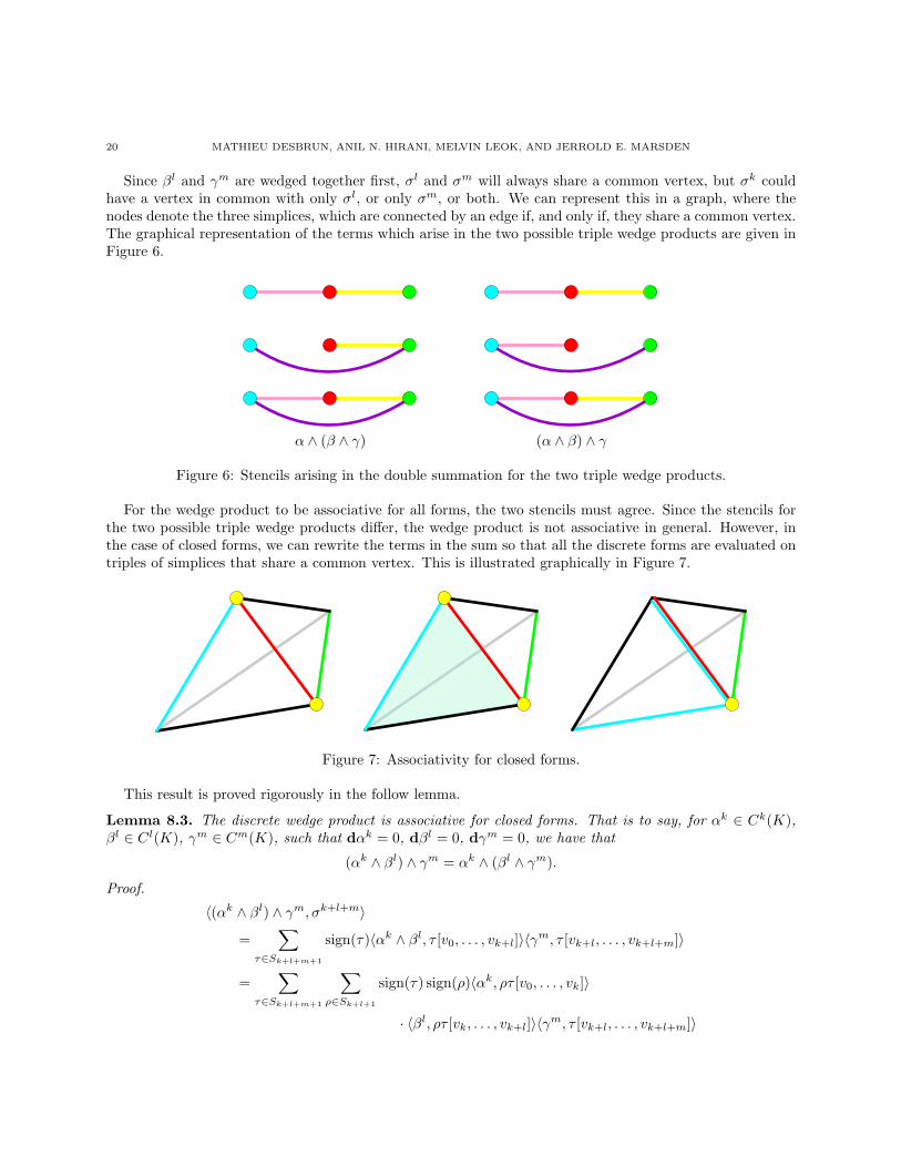
Associativity for the Wedge Product. The discrete wedge product which we have introduced is notassociative in general. This is a consequence of the fact that the stencil for the two possible triple wedgeproducts are not the same. In the expression for 〈αk∧(βl∧γm), σk+l+m〉, each term in the double summationconsists of a geometric factor multiplied by 〈αk, σk〉〈βl, σl〉〈γm, σm〉 for some k, l,m simplices σk, σl, σm.
20 MATHIEU DESBRUN, ANIL N. HIRANI, MELVIN LEOK, AND JERROLD E. MARSDEN
Since βl and γm are wedged together first, σl and σm will always share a common vertex, but σk couldhave a vertex in common with only σl, or only σm, or both. We can represent this in a graph, where thenodes denote the three simplices, which are connected by an edge if, and only if, they share a common vertex.The graphical representation of the terms which arise in the two possible triple wedge products are given inFigure 6.
α ∧ (β ∧ γ) (α ∧ β) ∧ γ
Figure 6: Stencils arising in the double summation for the two triple wedge products.
For the wedge product to be associative for all forms, the two stencils must agree. Since the stencils forthe two possible triple wedge products differ, the wedge product is not associative in general. However, inthe case of closed forms, we can rewrite the terms in the sum so that all the discrete forms are evaluated ontriples of simplices that share a common vertex. This is illustrated graphically in Figure 7.
Figure 7: Associativity for closed forms.
This result is proved rigorously in the follow lemma.
Lemma 8.3. The discrete wedge product is associative for closed forms. That is to say, for αk ∈ Ck(K),βl ∈ Cl(K), γm ∈ Cm(K), such that dαk = 0, dβl = 0, dγm = 0, we have that
(αk ∧ βl) ∧ γm = αk ∧ (βl ∧ γm).
Proof.
〈(αk ∧ βl) ∧ γm, σk+l+m〉
=∑
τ∈Sk+l+m+1
sign(τ)〈αk ∧ βl, τ [v0, . . . , vk+l]〉〈γm, τ [vk+l, . . . , vk+l+m]〉
=∑
τ∈Sk+l+m+1
∑ρ∈Sk+l+1
sign(τ) sign(ρ)〈αk, ρτ [v0, . . . , vk]〉
· 〈βl, ρτ [vk, . . . , vk+l]〉〈γm, τ [vk+l, . . . , vk+l+m]〉

DISCRETE EXTERIOR CALCULUS 21
Here, either ρτ(k) = τ(k + l), in which case all three permuted simplices share vτ(k+l) as a common vertex,or we need to rewrite either 〈αk, ρτ [v0, . . . , vk]〉 or 〈βl, ρτ [vk, . . . , vk+l]〉, using the fact that αk and βl areclosed forms.
If vτ(k+l) /∈ ρτ [v0, . . . , vk], then we need to rewrite 〈αk, ρτ [v0, . . . , vk]〉 by considering the simplex obtainedby adding the vertex vτ(k+l) to ρτ [v0, . . . , vk], which is [vτ(k+l), vρτ(0), . . . , vρτ(k)]. Then, since αk is closed,we have that
0 = 〈dαk, [vτ(k+l), vρτ(0), . . . , vρτ(k)]〉
= 〈αk, ∂[vτ(k+l), vρτ(0), . . . , vρτ(k)]〉
= 〈αk, [vρτ(0), . . . , vρτ(k)]〉 −k∑
i=0
(−1)i〈αk, [vτ(k+l), vρτ(0), . . . , vρτ(i), . . . , vρτ(k)]〉
or equivalently,
〈αk, [vρτ(0), . . . , vρτ(k)]〉 =k∑
i=0
(−1)i〈αk, [vτ(k+l), vρτ(0), . . . , vρτ(i), . . . , vρτ(k)]〉.
Notice that all the simplices in the sum, with the exception of the last one, will share two vertices, vτ(k+l)
and vρτ(k) with ρτ [vk, . . . , vk+l], and so their contribution in the triple wedge product will vanish due to theanti-symmetrized sum.
Similarly, if vτ(k+l) /∈ ρτ [vk, . . . , vk+l], using the fact that βl is closed yields
〈αk, [vρτ(k), . . . , vρτ(k+l)]〉 =k+l∑i=k
(−1)(i−k)〈αk, [vτ(k+l), vρτ(k), . . . , vρτ(i), . . . , vρτ(k+l)]〉.
As before, all the simplices in the sum, with the exception of the last one, will share two vertices, vτ(k+l)
and vρτ(k) with ρτ [v0, . . . , vk], and so their contribution in the triple wedge product will vanish due to theanti-symmetrized sum.
This allows us to rewrite the triple wedge product in the case of closed forms as
〈(αk ∧ βl) ∧ γm, σk+l+m〉 =k+l+m∑
i=0
∑τ∈Sk+l+m
sign(ρiτ)〈αk, ρiτ [v0, . . . , vk]〉〈βl, ρiτ [v0, vk+1, . . . , vk+l]〉
· 〈γm, ρiτ [v0, vk+l+1, . . . , vk+l+m]〉 ,where τ ∈ Sk+l+m is thought of as acting on the set 1, . . . , k + l+m, and ρi is a transposition of 0 and i.A similar argument allows us to write αk ∧ (βl ∧ γm) in the same form, and therefore, the wedge product isassociative for closed forms.
Remark 8.1. This lemma is significant, since if we think of a constant smooth differential form, anddiscretize it to obtain a discrete differential form, this discrete form will be closed. As such, this lemmastates that in the infinitesimal limit, the discrete wedge product we have defined will be associative.
In practice, if we have a mesh with characteristic length ∆x, then we will have that1
|σk+l+m|〈αk ∧ (βl ∧ γm)− (αk ∧ βl) ∧ γm, σk+l+m〉 = O(∆x),
which is to say that the average of the associativity defect is of the order of the mesh size, and thereforevanishes in the infinitesimal limit.

22 MATHIEU DESBRUN, ANIL N. HIRANI, MELVIN LEOK, AND JERROLD E. MARSDEN
9. Divergence and Laplace–Beltrami
In this section, we will illustrate the application of some of the DEC operations we have previously definedto the construction of new discrete operators such as the divergence and Laplace–Beltrami operators.
Divergence. The divergence of a vector field is given in terms of the Lie derivative of the volume-form,by the expression, (div(X)µ = £Xµ. Physically, this corresponds to the net flow per unit volume of aninfinitesimal volume about a point.
We will define the discrete divergence by using the formulas defining them in the smooth exterior calculus.The divergence definition will be valid for arbitrary dimensions. The resulting expressions involve operatorsthat we have already defined and so we can actually perform some calculations to express these quantitiesin terms of geometric quantities. We will show that the resulting expression in terms of geometric quantitiesis the same as that derived by variational means in Tong et al. [2003].
Definition 9.1. For a discrete dual vector field X the divergence div(X) is defined to be
div(X) = −δX[ .
Remark 9.1. The above definition is a theorem in smooth exterior calculus. See, for example, page 458 ofAbraham et al. [1988].
As an example, we will now compute the divergence of a discrete dual vector field on a two-dimensionalsimplicial complex K, as illustrated in Figure 8.
Figure 8: Divergence of a discrete dual vector field.
A similar derivation works in higher dimensions, where one needs to be mindful of the sign that arisesfrom applying the Hodge star twice, ∗ ∗αk = (−1)k(n−k)αk. Since div(X) = −δX[, it follows that div(X) =∗d ∗X[. Since this is a primal 0-form it can be evaluated on a 0-simplex σ0, and we have that
〈div(x), σ0〉 = 〈∗d ∗X[, σ0〉 .Using the definition of discrete Hodge star, and the discrete generalized Stokes’ theorem, we get
1|σ0|
〈div(X), σ0〉 =1
| ? σ0|〈∗ ∗ d ∗X[, ?σ0〉
=1
| ? σ0|〈d ∗X[, ?σ0〉
=1
| ? σ0|〈∗X[, ∂(?σ0)〉 .

DISCRETE EXTERIOR CALCULUS 23
The second equality is obtained by applying the definition of the Hodge star, and the last equality is obtainedby applying the discrete generalized Stokes’ theorem. But,
∂(?σ0) =∑
σ1σ0
?σ1 ,
as given by the expression for the boundary of a dual cell in Equation 5.8. Thus,1|σ0|
〈div(X), σ0〉 =1
| ? σ0|〈∗X[,
∑σ1σ0
?σ1〉
=1
| ? σ0|∑
σ1σ0
〈∗X[, ?σ1〉
=1
| ? σ0|∑
σ1σ0
| ? σ1||σ1|
〈X[, σ1〉
=1
| ? σ0|∑
σ1σ0
| ? σ1||σ1|
∑σ2σ1
| ? σ1 ∩ σ2|| ? σ1|
X · ~σ1
=1
| ? σ0|∑
σ1σ0
∑σ2σ1
| ? σ1 ∩ σ2||σ1|
X · ~σ1
=1
| ? σ0|∑
σ1σ0
| ? σ1 ∩ σ2| (X · ~σ1
|σ1|) .
This expression has the nice property that the divergence theorem holds on any dual n-chain, which,as a set, is a simply connected subset of |K|. Furthermore, the coefficients we computed for the discretedivergence operator are the unique ones for which a discrete divergence theorem holds.
Laplace–Beltrami. The Laplace–Beltrami operator is the generalization of the Laplacian to curved spaces.In the smooth case the Laplace–Beltrami operator on smooth functions is defined to be ∇2 = div curl = δd.See, for example, page 459 of Abraham et al. [1988]. Thus, in the smooth case, the Laplace–Beltrami onfunctions is a special case of the more general Laplace–deRham operator, ∆ : Ωk(M) → Ωk(M), defined by∆ = dδ + δd.
As an example, we compute ∆f on a primal vertex σ0, where f ∈ Ω0d(K), and K is a (not necessarily
flat) triangle mesh in R3, as illustrated in Figure 9.This calculation is done below.
1|σ0|
〈∆f, σ0〉 = 〈δdf, σ0〉
= −〈∗d ∗ df, σ0〉
= − 1| ? σ0|
〈d ∗ df, ?σ0〉
= − 1| ? σ0|
〈∗df, ∂(?σ0)〉
= − 1| ? σ0|
〈∗df,∑
σ1σ0
?σ1〉
= − 1| ? σ0|
∑σ1σ0
〈∗df, ?σ1〉

24 MATHIEU DESBRUN, ANIL N. HIRANI, MELVIN LEOK, AND JERROLD E. MARSDEN
σ0
Figure 9: Laplace–Beltrami of a discrete function.
= − 1| ? σ0|
∑σ1σ0
| ? σ1||σ1|
〈df, σ1〉
= − 1| ? σ0|
∑σ1σ0
| ? σ1||σ1|
(f(v)− f(σ0)) ,
where ∂σ1 = v − σ0. But, the above is the same as the formula involving cotangents found by Meyer et al.[2002] without using discrete exterior calculus.
Another interesting aspect, which will be discussed in §12, is that the characterization of harmonic func-tions as those functions which vanish when the Laplace–Beltrami operator is applied is equivalent to thatobtained from a discrete variational principle using DEC as the means of discretizing the Lagrangian.
10. Contraction and Lie Derivative
In this section we will discuss some more operators that involve vector fields, namely contraction, and Liederivatives.
For contraction, we will first define the usual smooth contraction algebraically, by relating it to Hodgestar and wedge products. This yields one potential approach to defining discrete contraction. However, sincein the discrete theory we are only concerned with integrals of forms, we can use the interesting notion ofextrusion of a manifold by the flow of a vector field to define the integral of a contracted discrete differentialform.
We learned about this definition of contraction via extrusion from Bossavit [2002b], who goes on to definediscrete extrusion in his paper. Thus, he is able to obtain a definition of discrete contraction. Extrusionturns out to be a very nice way to define integrals of operators involving vector fields, and we will show howto define integrals of Lie derivatives via extrusion, which will yield discrete Lie derivatives.
Definition 10.1. Given a manifold M , and S, a k-dimensional submanifold of M , and a vector fieldX ∈ X(M), we call the manifold obtained by sweeping S along the flow of X for time t as the extrusion ofS by X for time t, and denote it by Et
X(S). The manifold S carried by the flow for time t will be denotedϕt
X(S).
Example 10.1. Figure 10 illustrates the 2-simplex that arises from the extrusion of a 1-simplex by a discretevector field that is interpolated using a linear shape function.
Contraction (Extrusion). We first establish an integral property of the contraction operator.

DISCRETE EXTERIOR CALCULUS 25
Figure 10: Extrusion of 1-simplex by a discrete vector field.
Lemma 10.1. ∫S
iXβ =d
dt
∣∣∣∣t=0
∫Et
X(S)
β
Proof. Prove instead that ∫ t
0
[∫Sτ
iXβ]dτ =
∫Et
X(S)
β .
Then, by first fundamental theorem of calculus, the desired result will follow. To prove the above, simplytake coordinates on S and carry them along with the flow and define the transversal coordinate to be theflow of X. This proof is sketched in Bossavit [2002b].
This lemma allows us to interpret contraction as being the dual, under the integration pairing betweenk-forms and k-volumes, to the geometric operation of extrusion. The discrete contraction operator is thengiven by
〈iXαk+1, σk〉 =d
dt
∣∣∣∣t=0
〈αk+1, EtX(σk)〉,
where the evaluation of the RHS will typically require that the discrete differential form and the discretevector field are appropriately interpolated.
Remark 10.1. Since the dynamic definition of the contraction operator only depends on the derivative ofpairing of the differential form with the extruded region, it will only depend on the vector field in the regionS, and not on its extension into the rest of the domain.
In addition, if the interpolation for the discrete vector field satisfies a superposition principle, then thediscrete contraction operator will satisfy a corresponding superposition principle.
Contraction (Algebraic). Contraction is an operator that allows one to combine vector fields and forms.For a smooth manifold M , the contraction of a vector field X ∈ X(M) with a (k + 1)-form α ∈ Ωk+1(M)is written as iXα, and for vector fields X1, . . . , Xk ∈ X(M), the contraction in smooth exterior calculus isdefined by
iXα(X1, . . . , Xk) = α(X,X1, . . . , Xk) .We define contraction by using an identity that is true in smooth exterior calculus. This identity originallyappeared in Hirani [2003], and we state it here with proof.
Lemma 10.2 (Hirani [2003]). Given a smooth manifold M of dimension n, a vector field X ∈ X(M), anda k-form α ∈ Ωk(M), we have that
iXα = (−1)k(n−k) ∗ (∗α ∧X[) .

26 MATHIEU DESBRUN, ANIL N. HIRANI, MELVIN LEOK, AND JERROLD E. MARSDEN
Proof. Recall that for a smooth function f ∈ Ω0(M), we have that iXα = f iXα. This, and the multilinearityof α, implies that it is enough to show the result in terms of basis elements. In particular, let τ ∈ Sn be apermutation of the numbers 1, . . . n, such that τ(1) < . . . < τ(k), and τ(k + 1) < . . . < τ(n). Let X = eτ(j),for some j ∈ 1, . . . , n. Then, we have to show that
ieτ(j)eτ(1) ∧ . . . ∧ eτ(k) = (−1)k(n−k) ∗ (∗(eτ(1) ∧ . . . ∧ eτ(k)) ∧ eτ(j)) .
It is easy to see that the LHS is 0 if j > k, and it is
(−1)j−1(eτ(1) ∧ . . . ∧ eτ(j) . . . ∧ eσ(k)) ,
otherwise, where eτ(j) means that eτ(j) is omitted from the wedge product. Now, on the RHS of Equa-tion 10.2, we have that
∗(eτ(1) ∧ . . . ∧ eτ(k)) = sign(τ)(eτ(k+1) ∧ . . . ∧ eτ(n)) .Thus, the RHS is equal to
(−1)k(n−k) sign(τ) ∗ (eτ(k+1) ∧ . . . ∧ eτ(n) ∧ eτ(j)) ,
which is 0 as required if j > k. So, assume that 1 ≤ j ≤ k. We need to compute
∗(eτ(k+1) ∧ . . . ∧ eτ(n) ∧ eτ(j)) ,
which is given bys eτ(1) ∧ . . . eτ(j) ∧ . . . ∧ eτ(k) ,
where the sign s = ±1, such that the equation,
s eτ(k+1) ∧ . . . ∧ eτ(n) ∧ eτ(j) ∧ eτ(1) ∧ . . . ∧ eτ(j) ∧ . . . ∧ eτ(k) = µ ,
holds for the standard volume-form, µ = e1 ∧ . . . ∧ en. This implies that
s = (−1)j−1(−1)k(n−k) sign(τ) .
Then, RHS = LHS as required.
Since we have expressions for the discrete Hodge star (∗), wedge product (∧), and flat ([), we have thenecessary ingredients to use the algebraic expression proved in the above lemma to construct a discretecontraction operator.
One has to note, however, that the wedge product is only associative for closed forms, and as a consequence,the Leibniz rule for the resulting contraction operator will only hold for closed forms as well. This is, however,sufficient to establish that the Leibniz rule for the discrete contraction will hold in the limit as the mesh isrefined.
Lie Derivative (Extrusion). As was the case with contraction, we will establish a integral identity thatallows the Lie derivative to be interpreted as the dual of a geometric operation on a volume. This involvesthe flow of a volume by a vector field, and it is illustrated in the following example.
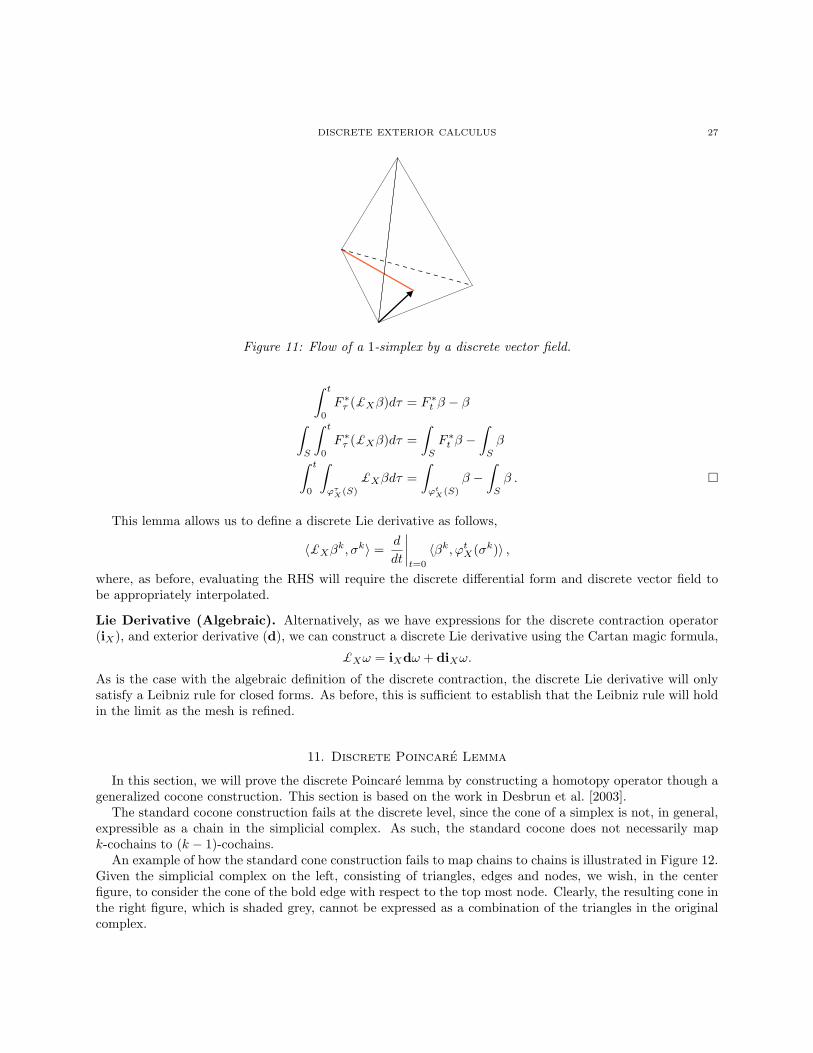
Example 10.2. Figure 11 illustrates the flow of a 1-simplex by a discrete vector field interpolated using alinear shape function.
Lemma 10.3. ∫S
£Xβ =d
dt
∣∣∣∣t=0
∫ϕt
X(S)
β .
Proof.
F ∗t (£Xβ) =d
dtF ∗t β
DISCRETE EXTERIOR CALCULUS 27
Figure 11: Flow of a 1-simplex by a discrete vector field.
∫ t
0
F ∗τ (£Xβ)dτ = F ∗t β − β∫S
∫ t
0
F ∗τ (£Xβ)dτ =∫
S
F ∗t β −∫
S
β∫ t
0
∫ϕτ
X(S)
£Xβdτ =∫
ϕtX(S)
β −∫
S
β .
This lemma allows us to define a discrete Lie derivative as follows,
〈£Xβk, σk〉 =
d
dt
∣∣∣∣t=0
〈βk, ϕtX(σk)〉 ,
where, as before, evaluating the RHS will require the discrete differential form and discrete vector field tobe appropriately interpolated.
Lie Derivative (Algebraic). Alternatively, as we have expressions for the discrete contraction operator(iX), and exterior derivative (d), we can construct a discrete Lie derivative using the Cartan magic formula,
£Xω = iXdω + diXω.
As is the case with the algebraic definition of the discrete contraction, the discrete Lie derivative will onlysatisfy a Leibniz rule for closed forms. As before, this is sufficient to establish that the Leibniz rule will holdin the limit as the mesh is refined.
11. Discrete Poincare Lemma
In this section, we will prove the discrete Poincare lemma by constructing a homotopy operator though ageneralized cocone construction. This section is based on the work in Desbrun et al. [2003].
The standard cocone construction fails at the discrete level, since the cone of a simplex is not, in general,expressible as a chain in the simplicial complex. As such, the standard cocone does not necessarily mapk-cochains to (k − 1)-cochains.
An example of how the standard cone construction fails to map chains to chains is illustrated in Figure 12.Given the simplicial complex on the left, consisting of triangles, edges and nodes, we wish, in the centerfigure, to consider the cone of the bold edge with respect to the top most node. Clearly, the resulting cone inthe right figure, which is shaded grey, cannot be expressed as a combination of the triangles in the originalcomplex.
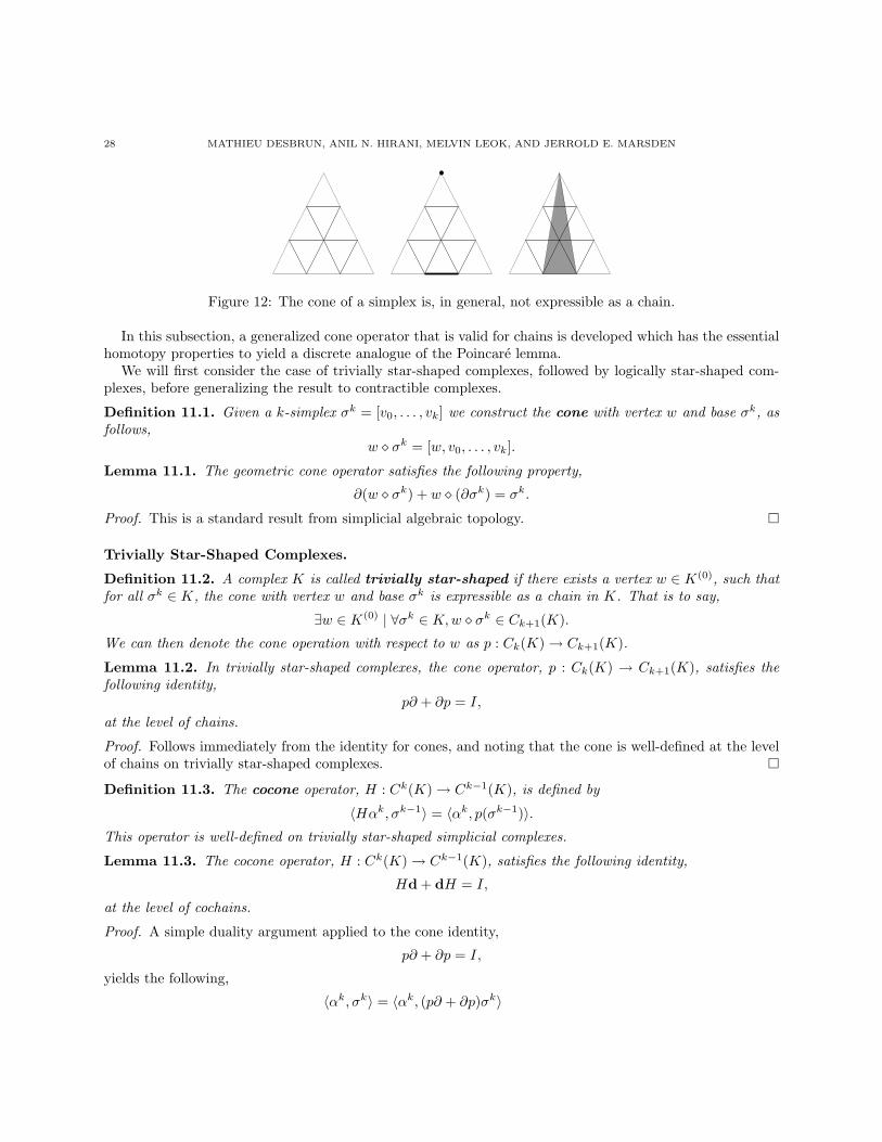
28 MATHIEU DESBRUN, ANIL N. HIRANI, MELVIN LEOK, AND JERROLD E. MARSDEN
Figure 12: The cone of a simplex is, in general, not expressible as a chain.
In this subsection, a generalized cone operator that is valid for chains is developed which has the essentialhomotopy properties to yield a discrete analogue of the Poincare lemma.
We will first consider the case of trivially star-shaped complexes, followed by logically star-shaped com-plexes, before generalizing the result to contractible complexes.
Definition 11.1. Given a k-simplex σk = [v0, . . . , vk] we construct the cone with vertex w and base σk, asfollows,
w σk = [w, v0, . . . , vk].
Lemma 11.1. The geometric cone operator satisfies the following property,
∂(w σk) + w (∂σk) = σk.
Proof. This is a standard result from simplicial algebraic topology.
Trivially Star-Shaped Complexes.
Definition 11.2. A complex K is called trivially star-shaped if there exists a vertex w ∈ K(0), such thatfor all σk ∈ K, the cone with vertex w and base σk is expressible as a chain in K. That is to say,
∃w ∈ K(0) | ∀σk ∈ K,w σk ∈ Ck+1(K).
We can then denote the cone operation with respect to w as p : Ck(K) → Ck+1(K).
Lemma 11.2. In trivially star-shaped complexes, the cone operator, p : Ck(K) → Ck+1(K), satisfies thefollowing identity,
p∂ + ∂p = I,
at the level of chains.
Proof. Follows immediately from the identity for cones, and noting that the cone is well-defined at the levelof chains on trivially star-shaped complexes.
Definition 11.3. The cocone operator, H : Ck(K) → Ck−1(K), is defined by
〈Hαk, σk−1〉 = 〈αk, p(σk−1)〉.This operator is well-defined on trivially star-shaped simplicial complexes.
Lemma 11.3. The cocone operator, H : Ck(K) → Ck−1(K), satisfies the following identity,
Hd + dH = I,
at the level of cochains.
Proof. A simple duality argument applied to the cone identity,
p∂ + ∂p = I,
yields the following,
〈αk, σk〉 = 〈αk, (p∂ + ∂p)σk〉
DISCRETE EXTERIOR CALCULUS 29
= 〈αk, p∂σk〉+ 〈αk, ∂pσk〉
= 〈Hαk, ∂σk〉+ 〈dαk, pσk〉
= 〈(dHαk, σk〉+ 〈Hdαk, σk〉
= 〈(dH +Hd)αk, σk〉.Therefore,
Hd + dH = I,
at the level of cochains.
Corollary 11.4 (Discrete Poincare Lemma for Trivially Star-shaped Complexes). Given a closed cochainαk, that is to say, dαk = 0, there exists a cochain βk−1, such that, dβk−1 = αk.
Proof. Applying the identity for cochains,
Hd + dH = I,
we have,
〈αk, σk〉 = 〈(Hd + dH)αk, σk〉 ,
but, dαk = 0, so,
〈αk, σk〉 = 〈d(Hαk), σk〉.
Therefore, βk−1 = Hαk is such that dβk−1 = αk at the level of cochains.
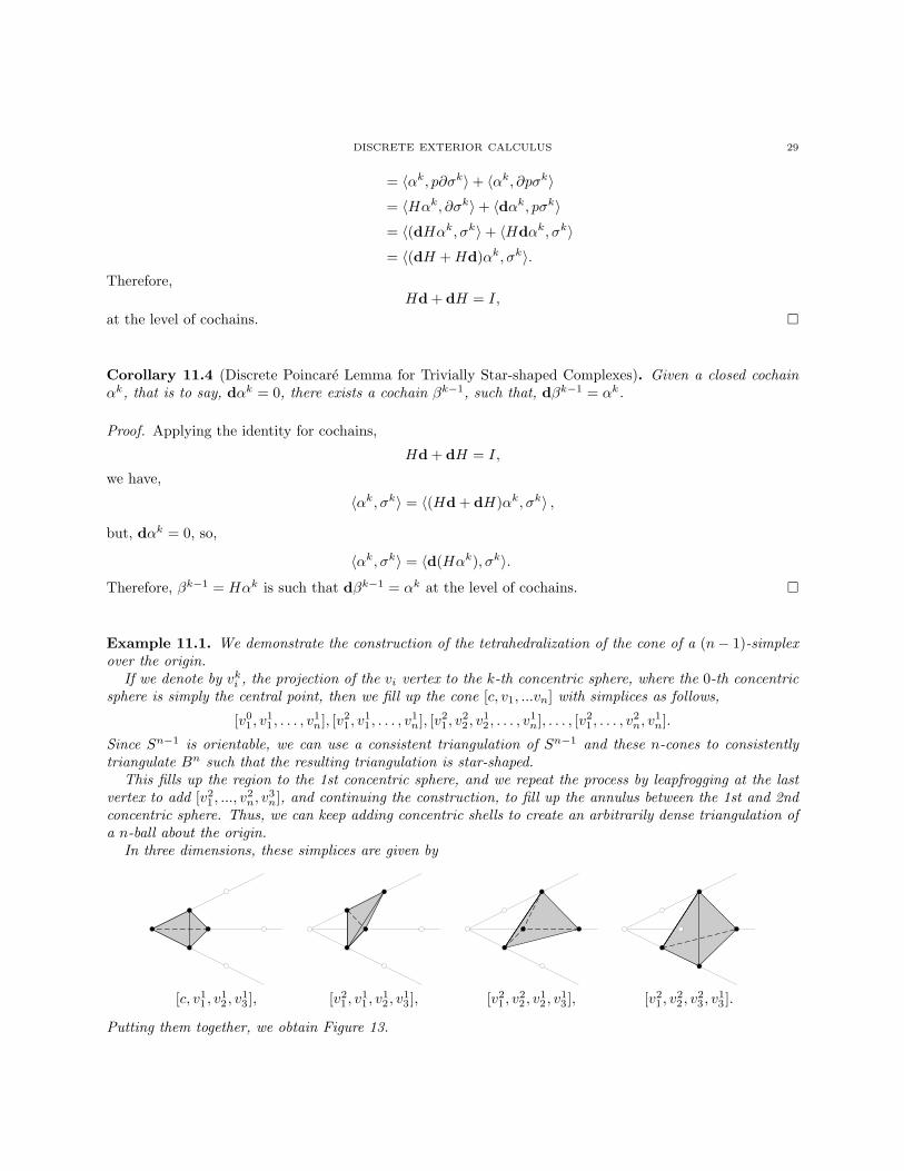
Example 11.1. We demonstrate the construction of the tetrahedralization of the cone of a (n− 1)-simplexover the origin.
If we denote by vki , the projection of the vi vertex to the k-th concentric sphere, where the 0-th concentric
sphere is simply the central point, then we fill up the cone [c, v1, ...vn] with simplices as follows,
[v01 , v
11 , . . . , v
1n], [v2
1 , v11 , . . . , v
1n], [v2
1 , v22 , v
12 , . . . , v
1n], . . . , [v2
1 , . . . , v2n, v
1n].
Since Sn−1 is orientable, we can use a consistent triangulation of Sn−1 and these n-cones to consistentlytriangulate Bn such that the resulting triangulation is star-shaped.
This fills up the region to the 1st concentric sphere, and we repeat the process by leapfrogging at the lastvertex to add [v2
1 , ..., v2n, v
3n], and continuing the construction, to fill up the annulus between the 1st and 2nd
concentric sphere. Thus, we can keep adding concentric shells to create an arbitrarily dense triangulation ofa n-ball about the origin.
In three dimensions, these simplices are given by
[c, v11 , v
12 , v
13 ], [v2
1 , v11 , v
12 , v
13 ], [v2
1 , v22 , v
12 , v
13 ], [v2
1 , v22 , v
23 , v
13 ].
Putting them together, we obtain Figure 13.

30 MATHIEU DESBRUN, ANIL N. HIRANI, MELVIN LEOK, AND JERROLD E. MARSDEN
Figure 13: Triangulation of a three-dimensional cone.
This example is significant, since we have demonstrated that for any n-dimensional ball about a point, wecan construct a trivially star-shaped triangulation of the ball, with arbitrarily high resolution. This allowsus to recover the smooth Poincare lemma in the limit of an infinitely fine mesh, using the discrete Poincarelemma for trivially star-shaped complexes.
Logically Star-Shaped Complexes.
Definition 11.4. A simplicial complex L is logically star-shaped if it is isomorphic, at the level of anabstract simplicial complex, to a trivially star-shaped complex K.
Example 11.2. We see two simplicial complexes, in Figure 14, which are clearly isomorphic as abstractsimplicial complexes.
∼=
Figure 14: Trivially star-shaped complex (left); Logically star-shaped complex (right).
Definition 11.5. The logical cone operator p : Ck(L) → Ck+1(L) is defined by making the followingdiagram commute,
Ck(K)pK // Ck+1(K)
Ck(L)pL // Ck+1(L)
Which is to say that, given the isomorphism ϕ : K → L, we define
pL = ϕ pK ϕ−1.

DISCRETE EXTERIOR CALCULUS 31
Example 11.3. We show an example of the construction of the logical cone operator.
pK //
pL //
This definition of the logical cone operator results in identities for the cone and cocone operator thatfollow from the trivially star-shaped case, and we record the results as follows.
Lemma 11.5. In logically star-shaped complexes, the logical cone operator satisfies the following identity,
p∂ + ∂p = I,
at the level of chains.
Proof. Follows immediately by pushing forward the result for trivially star-shaped complexes using theisomorphism.
Lemma 11.6. In logically star-shaped complexes, the logical cocone operator satisfies the following identity,
Hd + dH = I,
at the level of cochains.
Proof. Follows immediately by pushing forward the result for trivially star-shaped complexes using theisomorphism.
Similarly, we have a Discrete Poincare Lemma for logically star-shaped complexes.
Corollary 11.7 (Discrete Poincare Lemma for Logically Star-shaped Complexes). Given a closed cochainαk, that is to say, dαk = 0, there exists a cochain βk−1, such that, dβk−1 = αk.
Proof. Follows from the above lemma using the proof for the trivially star-shaped case.
Contractible Complexes. For arbitrary contractible complexes, we construct a generalized cone operatorsuch that it satisfies the identity,
p∂ + ∂p = I,
which is the crucial property of the cone operator, from the point of view of proving the discrete Poincarelemma.
The trivial cone construction gives a clue as to how to proceed in the construction of a generalized coneoperator. Notice that if a σk+1 is a term in p(σk), then p(σk+1) = ∅. This suggests how we can use thecone identity to inductively construct the generalized cone operator.

32 MATHIEU DESBRUN, ANIL N. HIRANI, MELVIN LEOK, AND JERROLD E. MARSDEN
To define p(σk), we consider σk+1 σk, such that, σk+1 and σk are consistently oriented. We applyp∂ + ∂p to σk+1. Then, we have
σk+1 = p(σk) + p(∂σk+1 − σk) + ∂p(σk+1).
If we set p(σk+1) = ∅,
σk+1 = p(σk) + p(∂σk+1 − σk) + ∂(∅)
= p(σk) + p(∂σk+1 − σk).
Rearranging, we havep(σk) = σk+1 − p(∂σk+1 − σk),
andp(σk+1) = ∅.
We are done, so long as the simplices in the chain ∂σk+1−σk already have p defined on it. This then reducesto enumerating the simplices in such a way that in the right hand side of the equation, we never evoke termsthat are undefined.
We now introduce a method of augmenting a complex so that the enumeration condition is always satisfied.
Definition 11.6. Given a n-complex K, consider a (n− 1)-chain cn−1 that is contained on the boundary ofK, and is included in the one-ring of some vertex on ∂K. Then, the one-ring cone augmentation of Kis the complex obtained by adding the n-cone w cn−1, and all its faces to the complex.
Definition 11.7. A complex is generalized star-shaped if it can be constructed by repeatedly applying theone-ring augmentation procedure.
We will explicitly show in Examples 11.4, and 11.7, how to enumerate the vertices in two and threedimensions. And in Examples 11.6, and 11.8, we will introduce regular triangulations of R2 and R3 that canbe constructed by inductive one-ring cone augmentation.
Remark 11.1. Notice that a non-contractible complex cannot be constructed by inductive one-ring coneaugmentation, since it will involve adding a cone to a vertex that has two disjoint base chains. This preventsus from enumerating the simplices in such as way that all the terms in ∂σk+1 − σk have had p defined onthem, and we see in Example 11.9 how this causes the cone identity, and hence the discrete Poincare lemmato break.
Example 11.4. In two dimensions, the one-ring condition implies that the base of the cone consists of eitherone or two 1-simplices. To aid in visualization, consider Figure 15.
Figure 15: One-ring cone augmentation of a complex in two dimensions.
In the case of one 1-simplex, [v0, v1], when we augment using the cone construction with the new vertexw, we define,
p([w]) = [v0, w] + p([v0]), p([v0, w]) = ∅,p([v1, w]) = [v0, v1, w]− p([v0, v1]), p([v0, v1, w]) = ∅.

DISCRETE EXTERIOR CALCULUS 33
In the case of two 1-simplices, [v0, v1], [v0, v2], we have,
p([w]) = [v0, w] + p([v0]), p([v0, w]) = ∅,p([v1, w]) = [v0, v1, w]− p([v0, v1]), p([v0, v1, w]) = ∅,p([v2, w]) = [v0, v2, w]− p([v0, v2]), p([v0, v2, w]) = ∅.
Example 11.5. We will now explicitly utilize the one-ring cone augmentation procedure to compute thegeneralized cone operator for part of a regular two-dimensional triangulation that is not logically star-shaped.
As a preliminary, we shall consider a logically star-shaped complex, and augment with a new vertex, asseen in Figure 16.
Figure 16: Logically star-shaped complex augmented by cone.
We use the logical cone operator for the subcomplex that is logically star-shaped, and the augmentationrules in the example above for the newly introduced simplices. This yields,
p
= + p
= ,
p
= ∅,
p
= + p
= + ∅
= ,
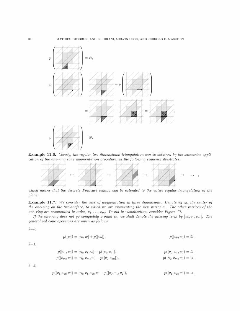
34 MATHIEU DESBRUN, ANIL N. HIRANI, MELVIN LEOK, AND JERROLD E. MARSDEN
p
= ∅,
p
= + p
= + = ,
p
= ∅.
Example 11.6. Clearly, the regular two-dimensional triangulation can be obtained by the successive appli-cation of the one-ring cone augmentation procedure, as the following sequence illustrates,
7→ 7→ 7→ 7→ . . . ,
which means that the discrete Poincare lemma can be extended to the entire regular triangulation of theplane.
Example 11.7. We consider the case of augmentation in three dimensions. Denote by v0, the center ofthe one-ring on the two-surface, to which we are augmenting the new vertex w. The other vertices of theone-ring are enumerated in order, v1, . . . , vm. To aid in visualization, consider Figure 17.
If the one-ring does not go completely around v0, we shall denote the missing term by [v0, v1, vm]. Thegeneralized cone operators are given as follows.
k=0,
p([w]) = [v0, w] + p([v0]), p([v0, w]) = ∅,
k=1,
p([v1, w]) = [v0, v1, w]− p([v0, v1]), p([v0, v1, w]) = ∅,p([vm, w]) = [v0, vm, w]− p([v0, vm]), p([v0, vm, w]) = ∅,
k=2,
p([v1, v2, w]) = [v0, v1, v2, w] + p([v0, v1, v2]), p([v1, v2, w]) = ∅,

DISCRETE EXTERIOR CALCULUS 35
Figure 17: One-ring cone augmentation of a complex in three dimensions.
p([vm−1, vm, w]) = [v0, vm−1, vm, w] + p([v0, vm−1, vm]), p([vm−1, vm, w]) = ∅.
If it does go around completely,
p([vm, v1, w]) = [v0, vm, v1, w] + p([v0, vm, v1]), p([v0, vm, v1, w]) = ∅.
Example 11.8. We provide a tetrahedralization of the unit cube that can be tiled to yield a regular tetrahe-dralization of R3. The 3-simplices are as follows,
[v000, v001, v010, v10], [v001, v010, v100, v101], [v001, v010, v011, v101],
[v010, v100, v101, v110], [v010, v011, v101, v110], [v011, v101, v110, v111].
The tetrahedralization of the unit cube can be seen in Figure 18.
(a) Tileable tetrahedralization of the unit cube (b) Partial tiling of R3
Figure 18: Regular tiling of R3 that admits a generalized cone operator.

36 MATHIEU DESBRUN, ANIL N. HIRANI, MELVIN LEOK, AND JERROLD E. MARSDEN
Since this regular tetrahedralization can be constructed by the successive application of the one-ring coneaugmentation procedure, the Discrete Poincare lemma can be extended to the entire regular tetrahedralizationof R3.
In higher dimensions, we can extend the construction of the generalized cone operator inductively usingthe one-ring cone augmentation by choosing an appropriate enumeration of the base chain. Topologically,the base chain will be the cone of Sn−2 (with possibly an open (n − 2)-ball removed) with respect to thecentral point.
By spiraling around Sn−2, starting from around the boundary of the n− 2 ball, and covering the rest ofSn−2, as in Figure 19, we obtain the higher-dimensional generalization of the procedure we have taken inExamples 11.4, and 11.7.
Figure 19: Spiral enumeration of Sn−2, n = 4.
Notice that n = 2 is distinguished, since S2−2 = S0 is disjoint, which is why in the two-dimensional case,we were not able to use the spiraling technique to enumerate the simplices.
Since we have constructed the generalized cone operator such that the cone identity holds, we have,
Lemma 11.8. In generalized star-shaped complexes, the generalized cone operator satisfies the followingidentity,
p∂ + ∂p = I,
at the level of chains.
Proof. By construction.
Lemma 11.9. In generalized star-shaped complexes, the generalized cocone operator satisfies the followingidentity,
Hd + dH = I,
at the level of cochains.
Proof. Follows immediately from applying the proof in the trivially star-shaped case, and using the identityin the previous lemma.
Similarly, we have a discrete Poincare lemma for generalized star-shaped complexes.
Corollary 11.10 (Discrete Poincare Lemma for Generalized Star-shaped Complexes). Given a closedcochain αk, that is to say, dαk = 0, there exists a cochain βk−1, such that, dβk−1 = αk.
Proof. Follows from the above lemma using the proof for the trivially star-shaped case.

DISCRETE EXTERIOR CALCULUS 37
Example 11.9. We will consider an example of how the Poincare lemma fails in the case when the complexis not contractible. Consider the following trivially star-shaped complex, and augment by one vertex so as tomake the region non-contractible, as show in Figure 20.
(a) Trivially star-shaped complex (b) Non-contractible complex
Figure 20: Counter-example for the discrete Poincare lemma for a non-contractible complex.
Now we attempt to verify the identity,p∂ + ∂p = I,
and we will see how this is only true up to a chain that is homotopic to the inner boundary.
(p∂ + ∂p)
= p
+
-
+ ∂
= +
= +
Since the second term cannot be expressed as the boundary of a 2-chain, it will contribute a non-trivial effect,even on closed discrete forms, and therefore the discrete Poincare lemma does not hold for non-contractiblecomplexes, as expected.
12. Discrete Variational Mechanics and DEC
We recall that discrete variational mechanics is based on a discrete analogue of Hamilton’s principle, andthey yield the discrete Euler–Lagrange equations. A particularly interesting property of DEC arises when itis used to construct the discrete Lagrangian for harmonic functions, and Maxwell’s equations.

38 MATHIEU DESBRUN, ANIL N. HIRANI, MELVIN LEOK, AND JERROLD E. MARSDEN
In particular, for these examples, the following diagram commutes,
LagrangianL : TQ→ R
DEC //
Discrete LagrangianLd : Q×Q→ R
Euler–LagrangeEL : T 2Q→ T ∗Q
DEC //Discrete Euler–Lagrange
ELd : Q3 → T ∗Q
Which is to say that directly discretizing the differential equations for harmonic functions, and Maxwell’sequations using DEC results in the same expressions as the discrete Euler–Lagrange equations associatedwith a discrete Lagrangian which is discretized from the corresponding continuous Lagrangian by using DECas the discretization scheme.
This is significant, since it implies that when DEC is used to discretize these equations, the correspondingnumerical scheme which is obtained is variational, and consequently exhibits excellent structure-preservingproperties.
In the variational principles for both harmonic functions and Maxwell’s equations, we require the L2 normobtained from the L2 inner product on Ωk(M), which is given by
〈αk, βk〉 =∫
M
α ∧ ∗β .
The discrete analogue of this requires a primal-dual wedge product, which is given below for forms ofcomplementary dimension.
Definition 12.1. Given a primal discrete k-form αk ∈ Ωkd(K), and a dual discrete (n − k)-form βn−k ∈
Ωn−kd (?K), the discrete primal-dual wedge product is defined as follows,
〈αk ∧ βn−k, Vσk〉 =|Vσk |
|σk|| ? σk|〈αk, σk〉〈βn−k, ?σk〉
=1n〈αk, σk〉〈βn−k, ?σk〉 ,
where Vσk is the n-dimensional support volume obtained by taking the convex hull of the simplex σk and itsdual cell ?σk.
The corresponding L2 inner product is as follows.
Definition 12.2. Given two primal discrete k-forms, αk, βk ∈ Ωkd(K), their discrete L2 inner product,
〈αk, βk〉d, is given by
〈αk, βk〉d =∑
σk∈K
|Vσk ||σk|| ? σk|
〈αk, σk〉〈∗β, ?σk〉
=1n
∑σk∈K
〈αk, σk〉〈∗β, ?σk〉 .
Remark 12.1. Notice that it would have been quite natural from the smooth theory to propose the followingmetric tensor 〈〈 , 〉〉 for differential forms,
〈 〈〈αk, βk〉〉v, Vσk〉 = |Vσk | 〈αk, σk〉|σk|
〈βk, σk〉|σk|
,

DISCRETE EXTERIOR CALCULUS 39
where the |Vσk | is the factor arising from integrating the volume-form over Vσk , and
〈αk, σk〉|σk|
〈βk, σk〉|σk|
is what we would expect for 〈〈αk, βk〉〉, if the forms αk and βk were constant on σk, which is the product ofthe average values of αk, and βk.
If we adopt this as our definition of the metric tensor for forms, we can recover the definition we obtainedin §6 for the Hodge star operator. Starting from the definition from the smooth theory,∫
〈〈αk, βk〉〉v =∫αk ∧ ∗βk ,
and expanding this in terms of the metric tensor for discrete forms, and the primal-dual wedge operator, weobtain
〈 〈〈αk, βk〉〉v, Vσk〉 = 〈αk ∧ ∗βk, Vσk〉 ,
|Vσk | 〈αk, σk〉|σk|
〈βk, σk〉|σk|
=|Vσk |
|σk|| ? σk|〈αk, σk〉〈∗βk, ?σk〉 .
When we eliminate common factors from both sides, we obtain the expression,1|σk|
〈βk, σk〉 =1
| ? σk|〈∗βk, ?σk〉 ,
which is the expression we previously obtained in Definition 6.1 of §6.
The L2 norm for discrete differential forms is given below.
Definition 12.3. Given a primal discrete k-form αk ∈ Ωkd(K), its discrete L2 norm is given by
‖αk‖2d = 〈αk, αk〉d
=1n
∑σk∈K
〈αk, σk〉〈∗αk, ?σk〉
=1n
∑σk∈K
| ? σk||σk|
〈αk, σk〉2 .
Given these definitions, we can now reproduce some computations that were originally shown in Castrillon-Lopez [2003].
Harmonic Functions. Harmonic functions φ : M → R can be characterized in a variational fashion asextremals of the following action functional,
S(φ) =12
∫M
‖dφ‖2v,
where v is a Riemannian volume-form in M . The corresponding Euler–Lagrange equation is given by
∗d ∗ dφ = −∆φ = 0,
which is the familiar characterization of harmonic functions in terms of the Laplace–Beltrami operator.The discrete action functional can be expressed in terms of the L2 norm we introduced above for discrete
forms,
Sd(φ) =12‖dφ‖2
d
=12n
∑σ1∈K
∣∣?σ1∣∣
|σ1|〈dφ, σ1〉2.

40 MATHIEU DESBRUN, ANIL N. HIRANI, MELVIN LEOK, AND JERROLD E. MARSDEN
The basic variations needed for the determination of the discrete Euler–Lagrange operator are obtained fromvariations that vary the value of the function φ at a given vertex v0, leaving the other values fixed. Thesevariations have the form,
φε = φ+ εη,
where η ∈ Ω0(M ; R) is such that 〈η, v0〉 = 1, and 〈η, v〉 = 0, for any v ∈ K(0)−v0. This family of variationsis enough to establish the variational principle. That is, we have
0 =d
dε
∣∣∣∣ε=0
Sd(φε)
=1n
∑σ1∈K
∣∣?σ1∣∣
|σ1|〈dφ, σ1〉〈dη, σ1〉
=1n
∑v0≺σ1
∣∣?σ1∣∣
|σ1|〈dφ, σ1〉 sgn(σ1; v0),(12.1)
where sgn(σ1; v) stands for the sign of σ1 with respect to v. Which is to say, sgn(σ1; v) = 1 if σ1 = [v′, v],and sgn(σ1; v) = −1 if σ1 = [v, v′]. On the other hand,
〈∗d ∗ dφ, v0〉 =1
| ? v0|〈d ∗ dφ, ?v0〉
=1
| ? v0|〈∗dφ, ∂ ? v0〉
=1
| ? v0|∑
v0≺σ1
〈∗dφ, ?σ1〉 sgn(σ1; v0)
=1
| ? v0|∑
v0≺σ1
| ? σ1||σ1|
〈dφ, σ1〉 sgn(σ1; v0),
where in the second to last equality, one has to note that the border of the dual cell of a vertex v0 consists,up to orientation, in the dual of all the 1-simplices starting from v0. This is illustrated in Figure 21, andfollows from a general expression for the boundary of a dual cell that was given in Definition 5.8.
The sign factor comes from the relation between the orientation of the dual of the 1-simplices and that of∂ ∗ v0. From this, we conclude that the variational discrete equation, given in Equation 12.1, is equivalentto the vanishing of the discrete Laplace–Beltrami operator,
∗d ∗ dφ = −∆ = 0.
Maxwell Equations. We can formulate the Maxwell equations of electromagnetism in a covariant fashionby considering the 1-form A (the potential) as our fundamental variable in a Lorentzian manifold X. Theaction functional for a Lagrangian formulation of electromagnetism is given by,
S(A) =12
∫X
‖dA‖2v ,
where ‖ · ‖ is the norm on forms induced by the Lorentzian metric on X, and v is the pseudo-Riemannianvolume-form. The 1-form A is related to the 4-vector potential encountered in the relativistic formulationof electromagnetism (see, for example Jackson [1998]).
The Euler–Lagrange equation corresponding to this action functional is given by
∗d ∗ dA = 0 .
In terms of the field strength, F = dA, the last equation is usually rewritten as
dF = 0 , ∗d ∗ F = 0 ,

DISCRETE EXTERIOR CALCULUS 41
(a) Vertex v (b) ?v (c) ∂ ? v
(d) σ1 v (e) ?σ1
Figure 21: Boundary of a dual cell.
which is the geometric formulation of the Maxwell equations.For the purposes of simplicity of exposition, we consider the special case where the Lorentzian manifold
decomposes into X = M×R, where (M, g) is a compact Riemannian 3-manifold. In formulating the discreteversion of this variational problem, we need to generalize the notion of a discrete Hodge dual to take intoaccount the pseudo-Riemannian metric structure. This can be subtle in practice, and to overcome this, weconsider a special family of complexes instead.
Let K ′ be a simplicial complex modelling M . For the sake of simplicity we consider M = R3 althoughthis is not strictly necessary. We now consider a discretization tnn∈Z of R. We define the complex K,modelling X = R4, the cells of which are the sets σ = σ′ × tn ⊂ R3 ×R, and σ = σ′ × (tn, tn+1) ⊂ R3 ×Rfor any σ′ ∈ K ′ and n ∈ Z. Of course, this is not a simplicial complex but rather a “prismal” complex, asshown in Figure 22.
The advantage of these cell complexes is the existence of the Voronoi dual. More precisely, given anyprismal cells σ′ × tn ∈ K and σ′ × (tn, tn+1) ∈ K, the Lorentz orthonormal to any of its edges coincidewith the Euclidean one in R4 and the existence of the circumcenter is thus guaranteed. In other words, theLorentz circumcentric dual ?K to K is the same as the Euclidean one in R4.
Remark 12.2. Much of the construction above can be carried out more generally by considering arbitrarycell complexes in R4 that are not necessarily prismal, as long as none of its 1-cells are lightlike. This causalitycondition is necessary to ensure that the circumcentric dual complex is well-behaved. However, it is sufficientfor computational purposes that the complex is well-centered, in the sense that the Lorentzian circumcenterof each cell is contained inside the cell. These issues will be addressed in future work.

42 MATHIEU DESBRUN, ANIL N. HIRANI, MELVIN LEOK, AND JERROLD E. MARSDEN
Space
Tim
eFigure 22: Prismal cell complex decomposition of space-time.
Recall that the Hodge star ∗ is uniquely defined by satisfying the following expression,
α ∧ ∗β = 〈〈α, β〉〉v ,for all α, β ∈ Ωk(X). The upshot of this is that the Hodge star operator depends on the metric, and sincewe have a pseudo-Riemannian metric, there is a sign that is introduced in our expression for the discreteHodge star (Definition 6.1) that depends on whether the cell it is applied to is either spacelike or timelike.The discrete Hodge star for prismal complexes in Lorentzian space is given below.
Definition 12.4. The discrete Hodge star for prismal complexes in Lorentzian space is a map∗ : Ωk
d(K) → Ωkd(∗K) defined by giving its action on cells in a prismal complex as follows,
1| ? σk|
〈∗αk, ?σk〉 = κ(σk)1|σk|
〈αk, σk〉,
where | · | stands for the volume and the causality sign κ(σk) is defined to be +1 if all the edges of σk arespacelike, and −1 otherwise.
The causality sign of 2-cells in a (2 + 1)-space-time is summarized in Table 4. We should note that thecausality sign for a 0-simplex, κ(σ0), is always 1. This is because a 0-simplex has no edges, and as such thestatement that all of its edges are spacelike is trivially true.
Table 4. Causality sign of 2-cells in a (2 + 1)-space-time.
σ2
κ(σ2) +1 +1 −1 −1 −1
This causality term in the discrete Hodge star has consequences for the expression for the discrete norm(Definition 12.3), which is now given.
DISCRETE EXTERIOR CALCULUS 43
Definition 12.5. Given a primal discrete k-form αk ∈ Ωkd(K), its discrete L2 Lorentzian norm is given
by,
‖αk‖2Lor,d =
1n
∑σk∈K
〈αk, σk〉〈∗αk, ?σk〉
=1n
∑σk∈K
κ(σk)| ? σk||σk|
〈αk, σk〉2 .
Having defined the discrete Lorentzian norm, we can express the discrete action as
Sd(A) =12‖dA‖2
Lor,d
=18
∑σ2∈K
〈dA, σ2〉〈∗dA, ?σ2〉
=18
∑σ2∈K
κ(σ2)| ? σ2||σ2|
〈dA, σ2〉2 .
The basic variations needed to determine the discrete Euler–Lagrange operator are obtained from variationsthat vary the value of the 1-form A at a given 1-simplex σ1
0 , leaving the other values fixed. These variationshave the form,
Aε = Aε + εη,
where η ∈ Ω1d(K) is given by 〈η, σ1
0〉 = 1 for a fixed interior σ10 ∈ K and 〈η, σ1〉 = 0 for σ1 6= σ1
0 . Thederivation of the variational principle gives
d
dε
∣∣∣∣ε=0
Sd(Aε) =14
∑σ2∈K
| ? σ2||σ2|
κ(σ2)〈dA, σ2〉〈dη, σ2〉
=14
∑σ10≺σ2
| ? σ2||σ2|
κ(σ2)〈dA, σ2〉〈dη, σ2〉
=14
∑σ10≺σ2
| ? σ2||σ2|
κ(σ2)〈dA, σ2〉 sgn(σ2, σ10),
which vanishes for all the basic variations above. On the other hand, we now expand the discrete 1-form∗d ∗ dA. For any σ1
0 ∈ K, we have that
〈∗d ∗ dA, σ10〉 =
|σ10 |
| ? σ10 |κ(σ1
0)〈d ∗ dA, ?σ10〉
=|σ1
0 || ? σ1
0 |κ(σ1
0)〈∗dA, ∂ ? σ10〉
=|σ1
0 || ? σ1
0 |κ(σ1
0)∑
σ10≺σ2
sgn(σ2, σ10)〈∗dA, ?σ2〉
=|σ1
0 || ? σ1
0 |κ(σ1
0)∑
σ10≺σ2
| ? σ2||σ2|
κ(σ2)〈dA, σ2〉 sgn(σ2, σ10),
where the sign sgn(σ2, σ1) stands for the relative orientation between σ2 and σ1. Which is to say, sgn(σ2, σ1) =1 if the orientation induced by σ2 on σ1 coincides with the orientation of σ1, and sgn(σ2, σ1) = −1 other-wise. For the second to last equality, one has to note that the border of the dual cell of an edge σ1
0 consists,conveniently oriented with the sgn operator, of the union of the duals of all the 2-simplices containing σ1
0 .

44 MATHIEU DESBRUN, ANIL N. HIRANI, MELVIN LEOK, AND JERROLD E. MARSDEN
This statement is the content of Definition 5.8, which gives the expression for the boundary of a dual cell,and was illustrated in Figure 21 for the case of n-dimensional dual cells.
By comparing the two computations, we find that for an arbitrary choice of σ10 ∈ K, 〈∗d ∗ dA, σ1
0〉 isequal (up to a non-zero constant) to δSd(A), which always vanishes. It follows that the variational discreteequations obtained above is equivalent to the discrete Maxwell equations,
∗d ∗ dA = 0.
13. Extensions to Dynamic Problems
It is desirable to leverage the exactness properties of the operators of discrete exterior calculus to constructnumerical algorithms with discrete conservation properties. For these purposes, it is appropriate to extendthe scope of DEC to incorporate dynamical behavior, by addressing the issue of discrete diffeomorphismsand flows.
As discussed in the previous section, DEC and discrete mechanics have interesting synergistic proper-ties, and in this section we will explore a groupoid interpretation of discrete mechanics that is particularlyappropriate to formulating the notion of pull-back and push-forward of discrete differential forms.
13.1. Groupoid Interpretation of Discrete Variational Mechanics. The groupoid formulation of dis-crete mechanics is particularly fruitful and natural, and it serves as a unifying tool for understanding thevariational formulation of discrete Lagrangian mechanics, and discrete Euler–Poincare reduction, as discussedin the work of Weinstein [1996] and Marsden et al. [1999, 2000].
The groupoid interpretation of discrete mechanics is most clearly illustrated if we consider the discretiza-tion of trajectories on TQ in two stages. Given a curve γ : R+ → TQ, we consider a discrete sampling givenby
gi = γ(ih) ∈ TQ.We then approximate TQ by Q×Q, and associate to gi two elements in Q. We denote this by
gi 7→ (q0i , q1i ).
Or equivalently, in the language of groupoids, see Cannas da Silva and Weinstein [1999], Weinstein [2001],we have
G
α
β
Q
where α is the source map, and β is the target map. Then,
gi 7→ (α(gi), β(gi)) = (q0i , q1i ).
This can be visualized as
q0i = α(gi) q1i = β(gi)• •!!
gi
A product · : G(2) → G is defined on the set of composable pairs,
G(2) := (g, h) ∈ G×G | β(g) = α(h).The groupoid composition g · h is defined by
α(g · h) = α(g),
β(g · h) = β(h).

DISCRETE EXTERIOR CALCULUS 45
This can be represented graphically as follows,
•α(g) = α(g · h)
•β(g) = α(h)
•β(h) = β(g · h)
g
!!
h
!!
g·h
!!
The set of composable pairs is the discrete analogue of the set of second-order curves on TQ. A curveγ : R+ → TQ is said to be second-order if there exists a curve q : R+ → Q, such that,
γ(t) = (q(t), q(t)).
The corresponding condition for discrete curves is that given a sequence of points inQ×Q, (q01 , q11), . . . , (q0p, q
1p),
we require thatq1i = q0i+1.
This implies that the discrete curve on Q×Q is derived from a (p+1)-pointed curve (q0, . . . , qp) on Q, where
qi =
q0i+1, if 0 ≤ i < p;q1i , if i = p.
This condition has a direct equivalent in groupoids,
β(gi) = q1i = q0i+1 = α(gi+1).
Which is to say that the sequence of points in Q × Q are composable. In general, this hierarchy of sets isdenoted by
G(p) := (g1, . . . , gp) ∈ Gp | β (gi) = α (gi+1) ,where G(0) ' Q.
In addition, the groupoid inverse is defined by the following,
α(g−1) = β(g),
β(g−1) = α(g).
This is represented as follows,
β(g−1) = α(g) α(g−1) = β(g)• •
g
!!
g−1
aa v
ng_XPI
Visualizing Groupoids. In summary, composition of groupoid elements, and the inverse of groupoidelements can be illustrated by Figure 23. As we will see in the next subsection, representing discretediffeomorphisms as pair groupoids is the natural method of ensuring that the mesh remains nondegenerate.
13.2. Discrete Diffeomorphisms and Discrete Flows. We will adopt the point of view of representinga discrete diffeomorphism as a groupoid, which was first introduced in Pekarsky and West [2003], andappropriately modify it to reflect the simplicial nature of our mesh. In addition, we will address the inducedaction of a discrete diffeomorphism on the dual mesh.
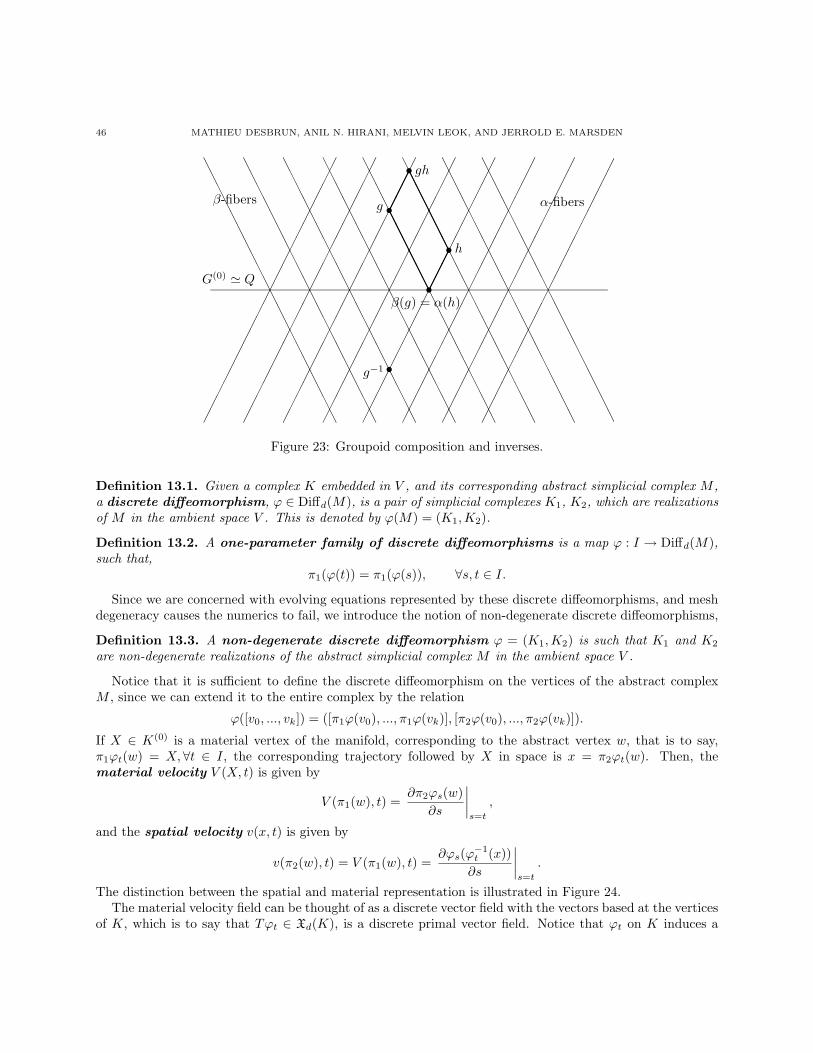
46 MATHIEU DESBRUN, ANIL N. HIRANI, MELVIN LEOK, AND JERROLD E. MARSDEN
β-fibersg
gh
h
β(g) = α(h)
α-fibers
g−1
G(0) ' Q
Figure 23: Groupoid composition and inverses.
Definition 13.1. Given a complex K embedded in V , and its corresponding abstract simplicial complex M ,a discrete diffeomorphism, ϕ ∈ Diffd(M), is a pair of simplicial complexes K1, K2, which are realizationsof M in the ambient space V . This is denoted by ϕ(M) = (K1,K2).
Definition 13.2. A one-parameter family of discrete diffeomorphisms is a map ϕ : I → Diffd(M),such that,
π1(ϕ(t)) = π1(ϕ(s)), ∀s, t ∈ I.
Since we are concerned with evolving equations represented by these discrete diffeomorphisms, and meshdegeneracy causes the numerics to fail, we introduce the notion of non-degenerate discrete diffeomorphisms,
Definition 13.3. A non-degenerate discrete diffeomorphism ϕ = (K1,K2) is such that K1 and K2
are non-degenerate realizations of the abstract simplicial complex M in the ambient space V .
Notice that it is sufficient to define the discrete diffeomorphism on the vertices of the abstract complexM , since we can extend it to the entire complex by the relation
ϕ([v0, ..., vk]) = ([π1ϕ(v0), ..., π1ϕ(vk)], [π2ϕ(v0), ..., π2ϕ(vk)]).
If X ∈ K(0) is a material vertex of the manifold, corresponding to the abstract vertex w, that is to say,π1ϕt(w) = X,∀t ∈ I, the corresponding trajectory followed by X in space is x = π2ϕt(w). Then, thematerial velocity V (X, t) is given by
V (π1(w), t) =∂π2ϕs(w)
∂s
∣∣∣∣s=t
,
and the spatial velocity v(x, t) is given by
v(π2(w), t) = V (π1(w), t) =∂ϕs(ϕ−1
t (x))∂s
∣∣∣∣s=t
.
The distinction between the spatial and material representation is illustrated in Figure 24.The material velocity field can be thought of as a discrete vector field with the vectors based at the vertices
of K, which is to say that Tϕt ∈ Xd(K), is a discrete primal vector field. Notice that ϕt on K induces a

DISCRETE EXTERIOR CALCULUS 47
E1
E2
E3
X
e1
e2
e3
x
ϕ
Figure 24: Spatial and material representations.
map ?ϕt on the vertices of the dual ?K, by the following,
?ϕt(c[v0, . . . , vn]) = (c[π1ϕt(v0), . . . , π1ϕt(vn)], c[π2ϕt(v0), . . . , π2ϕt(vn)]).
Similarly then, T ? ϕt ∈ Xd(?K) is a discrete dual vector field.
Comparison with Interpolatory Methods. At first glance, the groupoid formulation seems like acumbersome way to define a one-parameter family of discrete diffeomorphisms, and one may be tempted tothink of extending ϕt to the ambient space. We would then be thinking of ϕt : V → V . This is undesirablesince given ϕt and ψs which are non-degenerate flows, their composition ϕt ψs, which is defined, may resultin a degenerate mesh when applied to K. Thus, non-degenerate flows are not closed under this notion ofcomposition.
If we adopt groupoid composition instead at the level of vertices, we can always be sure that if we composetwo nondegenerate discrete diffeomorphisms, they will remain a nondegenerate discrete diffeomorphism.
Discrete Diffeomorphisms as Pair Groupoids. The space of discrete diffeomorphisms naturally hasthe structure of a pair groupoid. The discrete analogue of T Diff(M) from the point of view of temporaldiscretization is the pair groupoid Diff(M) × Diff(M). In addition, we discretize Diff(M) using Diffd(M),which is in turn a pair groupoid involving realizations of an abstract simplicial complex in an ambient space.
13.3. Push-Forward and Pull-Back of Discrete Vector Fields and Discrete Forms. For us toconstruct a discrete theory of exterior calculus that admits dynamic problems, it is critical that we introducethe notion of push-forward and pull-back of discrete vector fields and discrete forms under a discrete flow.
Push-Forward and Pull-Back of Discrete Vector Fields.The push-forward of a discrete vector field satisfies the following commutative diagram,
K? //
f
?KX //
?f
RN
Tf
L? // ?L
f∗X// RN
and the pull-back satisfies the following commutative diagram,
K? //
f
?Kf∗X
//
?f
RN
Tf
L? // ?L
X // RN
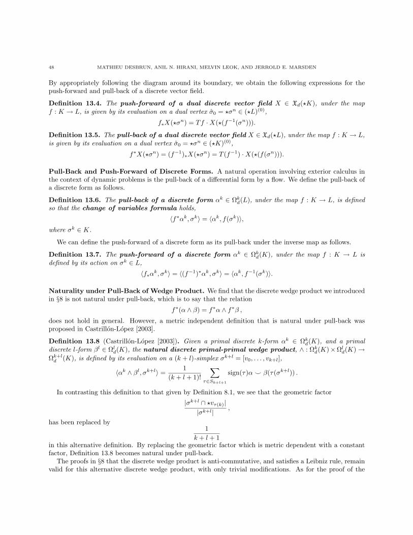
48 MATHIEU DESBRUN, ANIL N. HIRANI, MELVIN LEOK, AND JERROLD E. MARSDEN
By appropriately following the diagram around its boundary, we obtain the following expressions for thepush-forward and pull-back of a discrete vector field.
Definition 13.4. The push-forward of a dual discrete vector field X ∈ Xd(?K), under the mapf : K → L, is given by its evaluation on a dual vertex σ0 = ?σn ∈ (?L)(0),
f∗X(?σn) = Tf ·X(?(f−1(σn))).
Definition 13.5. The pull-back of a dual discrete vector field X ∈ Xd(?L), under the map f : K → L,is given by its evaluation on a dual vertex σ0 = ?σn ∈ (?K)(0),
f∗X(?σn) = (f−1)∗X(?σn) = T (f−1) ·X(?(f(σn))).
Pull-Back and Push-Forward of Discrete Forms. A natural operation involving exterior calculus inthe context of dynamic problems is the pull-back of a differential form by a flow. We define the pull-back ofa discrete form as follows.
Definition 13.6. The pull-back of a discrete form αk ∈ Ωkd(L), under the map f : K → L, is defined
so that the change of variables formula holds,
〈f∗αk, σk〉 = 〈αk, f(σk)〉,where σk ∈ K.
We can define the push-forward of a discrete form as its pull-back under the inverse map as follows.
Definition 13.7. The push-forward of a discrete form αk ∈ Ωkd(K), under the map f : K → L is
defined by its action on σk ∈ L,
〈f∗αk, σk〉 = 〈(f−1)∗αk, σk〉 = 〈αk, f−1(σk)〉.
Naturality under Pull-Back of Wedge Product. We find that the discrete wedge product we introducedin §8 is not natural under pull-back, which is to say that the relation
f∗(α ∧ β) = f∗α ∧ f∗β ,does not hold in general. However, a metric independent definition that is natural under pull-back wasproposed in Castrillon-Lopez [2003].
Definition 13.8 (Castrillon-Lopez [2003]). Given a primal discrete k-form αk ∈ Ωkd(K), and a primal
discrete l-form βl ∈ Ωld(K), the natural discrete primal-primal wedge product, ∧ : Ωk
d(K)×Ωld(K) →
Ωk+ld (K), is defined by its evaluation on a (k + l)-simplex σk+l = [v0, . . . , vk+l],
〈αk ∧ βl, σk+l〉 =1
(k + l + 1)!
∑τ∈Sk+l+1
sign(τ)α ^ β(τ(σk+l)) .
In contrasting this definition to that given by Definition 8.1, we see that the geometric factor
|σk+l ∩ ?vτ(k)||σk+l|
,
has been replaced by1
k + l + 1in this alternative definition. By replacing the geometric factor which is metric dependent with a constantfactor, Definition 13.8 becomes natural under pull-back.
The proofs in §8 that the discrete wedge product is anti-commutative, and satisfies a Leibniz rule, remainvalid for this alternative discrete wedge product, with only trivial modifications. As for the proof of the

DISCRETE EXTERIOR CALCULUS 49
associativity of the wedge product for closed forms, we note the following identity,∑τ∈Sk+l+1
|σk+l ∩ ?vτ(k)||σk+l|
=∑
τ∈Sk+l+1
1k + l + 1
= (k + l)! ,
which is a crucial observation for the original proof to apply to the alternative wedge product.
14. Remeshing Cochains and Multigrid Extensions
It is sometimes desirable, particularly in the context of multigrid, multiscale, and multiresolution compu-tations, to be able to represent a discrete differential form which is given as a cochain on a prescribed mesh,as one which is supported on a new mesh. Given a differential form ωk ∈ Ωk(K), and a new mesh M suchthat |K| = |M |, we can define it at the level of cosimplices,
∀τk ∈M (k), 〈ωk, τk〉 =∑
σk∈K(k)
sgn(τk, σk)|Vτk ∩ Vσk |
|Vσk |〈ωk, σk〉,
and extend this by linearity to cochains. Here, sgn(τk, σk) is +1 if the orientation of τk and σk are consistent,and −1 otherwise. Since k-skeletons of meshes that are not related by subdivision may not have nontrivialintersections, intersections of support volumes are used in the remeshing formula, as opposed to intersectionsof the k-simplices.
We denote this transformation at the level of cochains as, TK,M : Ck(K) → Ck(M). This has the naturalproperty that if we have a k-volume Uk that can be represented as a chain in either the complex K or thecomplex M , that is to say, Uk = σk
1 + . . .+ σkl = τk
1 + . . .+ τkl , then we have
〈ωk, τk1 + . . .+ τk
m〉 =m∑
i=1
〈ω, τki 〉 =
m∑i=1
∑σk∈K(k)
sgn(τki , σ
k)|Vτk
i∩ Vσk |
|Vσk |〈ωk, σk〉
=m∑
i=1
l∑j=1
sgn(τki , σ
kj )|Vτk
i∩ Vσk
j|
|Vσkj|
〈ωk, σkj 〉
=l∑
j=1
m∑i=1
sgn(τki , σ
kj )|Vτk
i∩ Vσk
j|
|Vσkj|
〈ωk, σkj 〉
=l∑
j=1
〈ωk, σkj 〉 = 〈ωk, σk
1 + . . .+ σkl 〉.
Which is to say that the integral of the differential form over Uk is well-defined, and independent of therepresentation of the differential form.
Note that, in particular, if we choose to coarsen the mesh, the value the form takes on a cell in the coarsermesh is simply the sum of the values the form takes on the old cells of the fine mesh which make up the newcell in the coarser mesh.
Non-Flat Manifolds. The case of non-flat manifolds presents a challenge in remeshing akin to thatencountered in the discretization of differential forms. In particular, if the two meshes represent differentdiscretizations of a non-flat manifold, they will in general correspond to different polyhedral regions in theembedding space, and not have the same support region.
We assume that our discretization of the manifold is sufficiently fine that for every simplex, all its verticesare contained in some chart. Then, by using these local charts, we can identify support volumes in thecomputational domain with n-volumes in the manifold, and thereby make sense of the remeshing formula.

50 MATHIEU DESBRUN, ANIL N. HIRANI, MELVIN LEOK, AND JERROLD E. MARSDEN
15. Conclusions and Future Work
We have presented a framework for discrete exterior calculus using the cochain representation of discretedifferential forms, and introduced combinatorial representations of discrete analogues of differential operatorson discrete forms and discrete vector fields. The role of primal and dual cell complexes in the theory aredeveloped in detail. In addition, extensions to dynamic problems and multi-resolution computations arediscussed.
In the next few paragraphs, we will describe some of the future directions that emanate from the currentwork on discrete exterior calculus.
Relation to Computational Algebraic Topology Since we have introduced a discrete Laplace-deRhamoperator, one can hope to develop a discrete Hodge-deRham theory, and relate the deRham cohomology ofa simplicial complex to its simplicial cohomology.
Extensions to Non-Flat Manifolds. The intrinsic notion of what constitutes the discrete tangent spaceto a node on a non-flat mesh remains an open question. It is possible that this notion is related to a choiceof discrete connection on the mesh, and it is an issue that deserves further exploration.
Generalization to Arbitrary Tensors. The discretization of differential forms as cochains is particularlynatural, due to the pairing between forms and volumes by integration. When attempting to discretizean arbitrary tensor, the natural discrete analogue is unclear. In particular, while it is possible to expandan arbitrary tensor using the tensor product of covariant and contravariant one-tensors, this would becumbersome to represent on a mesh. In Leok et al. [2003], which is on discrete connections, we will see Liegroup-valued discrete 1-forms, and one possible method of discretizing a (p, q)-tensor that is alternating inthe contravariant indices, is to consider it as a (0, q)-tensor-valued discrete p-form.
It would be particularly interesting to explore this in the context of the elasticity complex (see, forexample, Arnold [2002]),
se(3) // C∞(Ω,R3) ε // C∞(Ω,S) J // C∞(Ω,S) div // C∞(Ω,R3) // 0 ,
where S is the space of 3× 3 symmetric matrices. One approach to discretize this was suggested in Arnold[2002], which cites the use of the Bernstein–Gelfand–Gelfand resolution in Eastwood [2000] to derive theelasticity complex from the deRham complex. Alternatively, it might be appropriate in the context of theelasticity complex to consider Lie algebra-valued discrete differential forms.
Convergence and Higher-Order Theories. The natural question from the point of view of numericalanalysis would be to carefully analyze the convergence properties of these discrete differential geometricoperators. In addition, higher-order analogues of the discrete theory of exterior calculus are desirable fromthe point of view of computational efficiency, but the cochain representation is attractive due to its conceptualsimplicity and the elegance of representing discrete operators as combinatorial operations on the mesh.
It would therefore be desirable to reconcile the two, by ensuring that high-order interpolation and com-binatorial operations are consistent. As a low-order example, Whitney forms, which are used to interpolatedifferential forms on a simplicial mesh, have the nice property that taking the Whitney form associated withthe coboundary of a simplicial cochain is equal to taking the exterior derivative of the Whitney form asso-ciated with the simplicial cochain. As such, the coboundary operation, which is a combinatorial operationakin to finite differences, is an exact discretization of the exterior derivative, when applied to the degrees offreedom associated to the finite-dimensional function space of Whitney forms.
It would be interesting to apply subdivision surface techniques to construct interpolatory spaces thatare compatible with differential geometric operations that are combinatorial operations on the degrees offreedom. This will result in a massively simplified approach to higher-order theories of discrete exterior

DISCRETE EXTERIOR CALCULUS 51
calculus, by avoiding the use of symbolic computation, which would otherwise be necessary to compute theaction of continuous exterior differential operators on the polynomial expansions for differential forms.
References
R. Abraham, J. E. Marsden, and T. S. Ratiu. Manifolds, Tensor Analysis and Applications, volume 75 ofApplied Mathematical Sciences. Springer-Verlag, second edition, 1988.
D. H. Adams. R-torsion and linking numbers from simplicial abelian gauge theories. arXiv, hep-th/9612009,1996.
D. N. Arnold. Differential complexes and numerical stability. In Proceedings of the International Congressof Mathematicians, Vol. I (Beijing, 2002), pages 137–157, Beijing, 2002. Higher Ed. Press.
A. Bossavit. Generalized finite differences in computational electromagnetics. Progress in ElectromagneticsResearch, PIER, 32:45–64, 2001.
A. Bossavit. Applied differential geometry (a compendium). URLhttp://www.icm.edu.pl/edukacja/mat/Compendium.php. (preprint), 2002a.
A. Bossavit. Extrusion, contraction: Their discretization via Whitney forms. (preprint), 2002b.A. Bossavit. On “generalized finite differences”: Discretization of electromagnetic problems. (preprint),
2002c.A. Cannas da Silva and A. Weinstein. Geometric Models for Noncommutative Algebras, volume 10 of Berkeley
Mathematics Lecture Notes. American Mathematical Society, 1999.M. Castrillon-Lopez. Discrete variational problems on forms. (in preparation), 2003.M. Desbrun, A. N. Hirani, M. Leok, and J. E. Marsden. Discrete Poincare lemma. Appl. Numer. Math.,
2003. (submitted).A. A. Dezin. Multidimensional Analysis and Discrete Models. CRC Press, 1995.M. Eastwood. A complex from linear elasticity. In The Proceedings of the 19th Winter School “Geometry
and Physics” (Srnı, 1999), number 63 in Rend. Circ. Mat. Palermo (2) Suppl., pages 23–29, 2000.R. Forman. Discrete Morse theory and the cohomology ring. Trans. Amer. Math. Soc., 354(12):5063–5085
(electronic), 2002.P. W. Gross and P. R. Kotiuga. Data structures for geometric and topological aspects of finite element
algorithms. Progress in Electromagnetics Research, PIER, 32:151–169, 2001.A. Hatcher. Algebraic Topology. Cambridge University Press, 2001.R. Hiptmair. Canonical construction of finite elements. Math. Comp., 68(228):1325–1346, 1999.R. Hiptmair. Discrete Hodge-operators: An algebraic perspective. Progress in Electromagnetics Research,
PIER, 32:247–269, 2001a.R. Hiptmair. Higher order Whitney forms. Progress in Electromagnetics Research, PIER, 32:271–299, 2001b.R. Hiptmair. Finite elements in computational electromagnetism. In Acta Numerica, volume 11, pages
237–339. Cambridge University Press, 2002.A. N. Hirani. Discrete Exterior Calculus. PhD thesis, California Institute of Technology, 2003.J. D. Jackson. Classical Electrodynamics. Wiley, third edition, 1998.T. Kaczynski, K. Mischaikow, and M. Mrozek. Computational homology, volume 157 of Applied Mathematical
Sciences. Springer-Verlag, 2004.M. Leok, J. E. Marsden, and A. Weinstein. A discrete theory of connections on principal bundles. (in
preparation), 2003.A. Lew, J. E. Marsden, M. Ortiz, and M. West. Asynchronous variational integrators. Arch. Ration. Mech.
An., 167(2):85–146, 2003.E. L. Mansfield and P. E. Hydon. On a variational complex for difference equations. In The Geometrical
Study of Differential Equations (Washington, DC, 2000), volume 285 of Contemporary Mathematics, pages121–129. American Mathematical Society, 2001.

52 MATHIEU DESBRUN, ANIL N. HIRANI, MELVIN LEOK, AND JERROLD E. MARSDEN
J. E. Marsden, S. Pekarsky, and S. Shkoller. Discrete Euler–Poincare and Lie–Poisson equations. Nonlin-earity, 12(6):1647–1662, 1999.
J. E. Marsden, S. Pekarsky, and S. Shkoller. Symmetry reduction of discrete Lagrangian mechanics on Liegroups. J. Geom. Phys., 36(1-2):140–151, 2000.
C. Mattiussi. An analysis of finite volume, finite element, and finite difference methods using some conceptsfrom algebraic topology. J. Comput. Phys., 133(2):289–309, 1997.
C. Mattiussi. The finite volume, finite difference, and finite element methods as numerical methods forphysical field problems. Adv. Imag. Elect. Phys., 113:1–146, 2000.
M. Meyer, M. Desbrun, P. Schroder, and A. H. Barr. Discrete differential-geometry operators for triangulated2-manifolds. VisMath, 2002.
B. Moritz. Vector Difference Calculus. PhD thesis, University of North Dakota, 2000.B. Moritz and W. A. Schwalm. Triangle lattice green functions for vector fields. J. Phys. A., 34(3):589–602,
2001.J. R. Munkres. Elements of Algebraic Topology. Addison-Wesley, 1984.R. A. Nicolaides and D. -Q. Wang. Convergence analysis of a covolume scheme for Maxwell’s equations in
three dimensions. Math. Comp., 67(223):947–963, 1998.S. Pekarsky and M. West. Discrete diffeomorphism groupoids and circulation conserving fluid integrators.
(in preparation), 2003.J. R. Schewchuck. What is a good linear finite element? Interpolation, conditioning, anisotropy and quality
measures. URL http://www.cs.berkeley.edu/~jrs/papers/elemj.ps. (preprint), 2002.W. A. Schwalm, B. Moritz, M. Giona, and M. K. Schwalm. Vector difference calculus for physical lattice
models. Phys. Rev. E., 59(1, part B):1217–1233, 1999.S. Sen, S. Sen, J. C. Sexton, and D. H. Adams. Geometric discretization scheme applied to the abelian
Chern–Simons theory. Phys. Rev. E, 61(3):3174–3185, 2000.F. L. Teixeira. Geometric aspects of the simplicial discretization of Maxwell’s equations. Progress in Elec-
tromagnetics Research, PIER, 32:171–188, 2001.Y. Y. Tong, S. Lombeyda, A. N. Hirani, and M. Desbrun. Discrete multiscale vector field decomposition.
ACM Transactions on Graphics (SIGGRAPH), July 2003.E. Tonti. Finite formulation of electromagnetic field. IEEE Trans. Mag., 38:333–336, 2002.A. Weinstein. Lagrangian mechanics and groupoids. In Mechanics Day (Waterloo, ON, 1992), volume 7 of
Fields Institute Communications, pages 207–231. American Mathematical Society, 1996.A. Weinstein. Groupoids: unifying internal and external symmetry. A tour through some examples. In
Groupoids in Analysis, Geometry, and Physics (Boulder, CO, 1999), volume 282 of Contemporary Math-ematics, pages 1–19. American Mathematical Society, 2001.
H. Whitney. Geometric Integration Theory. Princeton University Press, 1957.Z. J. Wood. Computational Topology Algorithms for Discrete 2-Manifolds. PhD thesis, California Institute
of Technology, 2003.
Computer Science, USC, 941 W. 37th Place Los Angeles, CA 90089.
E-mail address: [email protected]
256-80, Computer Science, Caltech, Pasadena, CA 91125.
E-mail address: [email protected]
107-81, Control and Dynamical Systems, Caltech, Pasadena, CA 91125.
E-mail address: [email protected]
107-81, Control and Dynamical Systems, Caltech, Pasadena, CA 91125.E-mail address: [email protected]


![DISCRETE EXTERIOR CALCULUS arXiv:math/0508341v2 ...arXiv:math/0508341v2 [math.DG] 18 Aug 2005 DISCRETE EXTERIOR CALCULUS MATHIEU DESBRUN, ANIL N. HIRANI, MELVIN LEOK, AND JERROLD E](https://img.dokumen.tips/doc/110x75/60b7a1cc2888b721ac372341/discrete-exterior-calculus-arxivmath0508341v2-arxivmath0508341v2-mathdg.jpg)


![Discretization of Maxwell-Vlasov Equations based on Discrete Exterior …1276... · 2017. 9. 28. · Maxwell-Vlasov equations based on discrete exterior cal-culus [3, 5, 6] and some](https://img.dokumen.tips/doc/110x75/60e079cee64c2b05b10a79ca/discretization-of-maxwell-vlasov-equations-based-on-discrete-exterior-1276.jpg)