Physica A 389 (2010) 4755–4768

Contents lists available at ScienceDirect

Physica A

journal homepage: www.elsevier.com/locate/physa

Discovering network behind infectious disease outbreakYoshiharu Maeno ∗Social Design Group, Tokyo, Japan

a r t i c l e i n f o

Article history:Received 31 March 2010Received in revised form 11 June 2010Available online 16 July 2010

Keywords:Epidemiological compartment modelMeta-population network modelMaximal likelihood estimationSevere Acute Respiratory SyndromeStochastic differential equation

a b s t r a c t

Stochasticity and spatial heterogeneity are of great interest recently in studying thespread of an infectious disease. The presented method solves an inverse problem todiscover the effectively decisive topology of a heterogeneous network and reveal thetransmission parameters which govern the stochastic spreads over the network from adataset on an infectious disease outbreak in the early growth phase. Populations in acombination of epidemiological compartment models and a meta-population networkmodel are described by stochastic differential equations. Probability density functions arederived from the equations and used for themaximal likelihood estimation of the topologyand parameters. The method is tested with computationally synthesized datasets and theWHO dataset on the SARS outbreak.

© 2010 Elsevier B.V. All rights reserved.

1. Introduction

When the epidemiologists at a public health agency detect a signal of an infectious disease outbreak, they rely heavily onmathematical models of disease transmission in estimating the rate of transmission, predicting the direction and speed ofthe spread, and figuring out an effective measure to contain the outbreak. Many of the models formulate stochasticity andspatial heterogeneity, which are of great interest recently. The spatial heterogeneity ranges from the uneven probabilitiesof contacts between the individuals in communities [1,2], dependence of the strength of the demographical interactionsbetween cities on the distance [3], to nation-wide or world-wide inhomogeneous geographical structures [4,5].AMonte-Carlo stochastic simulation is widely used to understand the influence of the spatial heterogeneity on stochastic

spreading. In such a simulation, accuracy and reproducibility of the input demographical knowledge such as the amount oftraffic between cities have great impacts on the reliability of the output pattern of the movement of pathogens and theirhosts. But, in studyingworld-wide epidemics, just a collection of regular airline routes and aircraft capacities does not alwayspresent the transportation network which results in the real chain of transmission. Some routes are influential decisively,but the others are not. Examples are found in the spread of Severe Acute Respiratory Syndrome (SARS) from Asia to theworld in 2003. There were not any cases in Japan in spite of the heavy traffic there from Asian countries. Many patientsappeared in Canada earlier than the United States to which airlines connect Asian countries muchmore densely. Here arisesan interesting question. Inversely, is it possible to learn the effectively decisive transportation network by observing howthe disease spreads, reinforce the demographical knowledge on the network, and import the acquired knowledge into themathematical model? This is an inverse problem similar to the network tomography [6,7].In this study, a statistical method is presented to discover the effectively decisive topology of a heterogeneous network

and reveal the parameters which govern stochastic transmission from a dataset on the early growth phase of the outbreak.The dataset consists of either the number of infectious persons or the number of new cases per an observation interval.The method is founded on a mathematical model for a stochastic reaction–diffusion process [8]. The population in the

∗ Corresponding address: Social Design Group, 1-6-38F Sengoku, Bunkyo-ku, Tokyo 112-0011, Japan.E-mail address:maeno.yoshiharu@socialdesigngroup.com.

0378-4371/$ – see front matter© 2010 Elsevier B.V. All rights reserved.doi:10.1016/j.physa.2010.07.014

4756 Y. Maeno / Physica A 389 (2010) 4755–4768

model is described by a set of Langevin equations. The equations are stochastic differential equations which include rapidlyfluctuating and highly irregular functions of time. Probability density functions and likelihood functions are derived fromthe equations analytically, and used for the maximal likelihood estimation of the topology and parameters. The method istested with a number of computationally synthesized datasets and the World Health Organization (WHO) dataset on theSARS outbreak in March through April in 2003.

2. Problem

2.1. Stochastic model

Themodel in this study is a special case of a stochastic reaction–diffusion process. Themodel is a combination of standardepidemiological SIR or SIS compartment models and a meta-population network model [9]. The meta-population networkmodel [10] sub-divides the entire population into distinct sub-populations in N geographical regions. Movement of personsoccurs between the sub-populations while the epidemiological state transitions (infection and recovery) occur in a sub-population. A sub-population is randomly well-mixed. Heterogeneity is present between sub-populations.The geographical regions are represented by nodes ni (i = 0, 1, . . . ,N−1). The movement is parameterized by a matrix

γ whose i-th row and j-th column element γij is the probability at which a person moves from ni to nj per a unit time. Aperson remains at the same node at the probability of 1−

∑N−1j=0 γij. Generally, γij = γji does not hold. By definition, γii = 0. It

is often confirmed empirically that a simple law relates a network topology to the movement [11]. The topology is specifiedby a neighbor matrix l. The transportation between two regions is represented by a pair of unidirectional links. If a pairof links is present between ni and nj, lij = lji = 1. If absent, lij = lji = 0. By definition, lii = 0. In the experiments inSection 4, an empirically confirmed law γij = Γij(l) is postulated, and the topology and the probability of movement aretreated interchangeably.The SIR compartmentmodel [12] is a behavioral extremewhere immunity is life-long. The state of a person changes from

a susceptible state (S), through an infectious state (I), to a recovered state (R). In contrast, the immunity does not occur inthe SIS compartment model. The state of a recovered patient goes back to S. The parameter α represents the probability atwhich an infectious person contacts a person and infect the person per a unit time. If the contacted person is susceptible, thenumber of the infectious persons increases by 1. The effective rate of infection by a single infectious person is the productof α and the proportion of the susceptible persons within the population. The parameter β represents the probability atwhich an infectious person recovers per a unit time. These parameters are constants over subpopulations and time. Thebasic reproductive ratio r is defined by r = α/β [13].Movement, infection and recovery are Markovian stochastic processes governed by γij, α, and β .

2.2. Time evolution of spread

In a stochastic process, even if the initial condition is known, there are many possible trajectories which the processmight go along. A set of these possible trajectories is a statistical ensemble. The change in the population is described by aset of Langevin equations [14]. A Langevin equation is a stochastic differential equation [15]. The microscopic continuoustime evolution of a system is obtained by adding a fluctuation (a stochastic term) to the knownmacroscopic time evolutionof the system.The quantity Si(t) is the number of susceptible persons at a node ni at time t . Ii(t) is the number of infectious persons.

Ri(t) is the number of recovered persons. The change in Ii(t) (i = 0, 1, . . . ,N − 1) is given by Eq. (1) [16]. It is a set of Nstochastic differential equations.

dIi(t)dt=

αSi(t)Ii(t)Si(t)+ Ii(t)+ Ri(t)

− βIi(t)+N−1∑j=0

γjiIj(t)−N−1∑j=0

γijIi(t)

+

√αSi(t)Ii(t)

Si(t)+ Ii(t)+ Ri(t)ξ[α]i (t)−

√βIi(t)ξ

[β]

i (t)+N−1∑j=0

√γjiIj(t)ξ

[γ ]

ji (t)−N−1∑j=0

√γijIi(t)ξ

[γ ]

ij (t). (1)

Stochastic terms ξ(t) = (ξ[α]i (t), ξ [β]i (t), ξ [γ ]ij (t)) are rapidly fluctuating and highly irregular functions of time. The

number of terms is M = N2 + N (N terms for infection, N terms for recovery, and N(N − 1) terms for movement). Thefunctional forms of individual elements ξa(t) (a = 0, 1, . . . ,M−1) are not known. Their statistical property is the Gaussianwhite noise which satisfies Eq. (2) through (4).

〈ξa(t)〉ensemble = 0 (2)〈ξa(t)ξb(u)〉ensemble = δabδ(u− t) (3)〈ξa(t)ξb(u)ξc(v) · · ·〉ensemble = 0. (4)

Y. Maeno / Physica A 389 (2010) 4755–4768 4757

In these equations, δ(t) is aDirac’s delta function, and δab is a Kronecker’s delta symbol. The ensemble average of a variablex is 〈x〉ensemble. Eq. (3) means that there is no correlation at different times and between different terms. Eq. (4) means thatthe third and higher order moments vanish.Inmost cases, the outbreak is contained before the spread reaches equilibrium. In the early growth phase of the outbreak,

Ii � Si and Ri � Si hold true. The first term of the rightside of Eq. (1) is independent of Si and Ri because Si/(Si+ Ii+Ri) ≈ 1.The resulting equation is Eq. (5). Eq. (5) can also be applied to the SIS model.

dIi(t)dt= αIi(t)− βIi(t)+

N−1∑j=0

γjiIj(t)−N−1∑j=0

γijIi(t)

+

√αIi(t)ξ

[α]i (t)−

√βIi(t)ξ

[β]

i (t)+N−1∑j=0

√γjiIj(t)ξ

[γ ]

ji (t)−N−1∑j=0

√γijIi(t)ξ

[γ ]

ij (t). (5)

The cumulative number of new cases until time t is represented by Ji(t) (i = 0, 1, . . . ,N−1). The rate of increase in Ji(t)equals to the first term of Eq. (5). That is, αIi(t). The time evolution of Ji(t) is given by Eq. (6). The rightside dose not dependon Ji(t) itself.

dJi(t)dt= αIi(t)+

√αIi(t)ξ

[α]i (t). (6)

The total number of the infectious persons at time t is given by I(t) =∑N−1i=0 Ii(t). Its time evolution is given by Eq. (7).

It does not depend on the values of γij.

dI(t)dt= αI(t)− βI(t)+

N−1∑i=0

√αIi(t)ξ

[α]i (t)−

N−1∑i=0

√βIi(t)ξ

[β]

i (t). (7)

The total cumulative number of new cases until time t is given by J(t) =∑N−1i=0 Ji(t). Its time evolution is given by Eq.

(8).

dJ(t)dt= αI(t)+

N−1∑i=0

√αIi(t)ξ

[α]i (t). (8)

2.3. Definition of problem

The problem is to discover the network topology l (or γ) and reveal the transmission parameter r (or α and β) from agiven dataset Ii(td) (i = 0, 1, . . . ,N − 1, d = 0, 1, . . . ,D − 1) or1Ji(td) (i = 0, 1, . . . ,N − 1, d = 0, 1, . . . ,D − 1). Thedataset Ii(td) is the time sequence of the number of infectious persons. The dataset 1Ji(td) = Ji(td+1) − Ji(td) is the timesequence of the number of new cases between observations. An observation is made at every node ni (i = 0, 1, . . . ,N − 1)at times td (d = 0, 1, . . . ,D − 1). The time interval between observations is 1t = td+1 − td. For example, a bundle of thedaily reports on cases from hospitals is a dataset1Ji(td)where1t = 1 day. Other information is not known. That is, nothingis known about Si(td), Ri(td), nor the initial condition which could identify the index case (the first patient from whom theinfectious disease has spread).

3. Method

3.1. Likelihood function

Various techniques of statistical inference can be applied once the likelihood function is obtained analytically. Thelikelihood function is the conditional probability of the obtained dataset as a function of the unknown parameters of aparameterized statistical model. The conditional probability becomes noticeably large if the value of the parameters is closeto the true value. For example, maximal a posteriori estimation is used to find the parameters whichmaximize the posteriordistribution. In this study, the problem is solved by maximal likelihood estimation. The Langevin equation (5) through(8) are solved by obtaining the moments of probability variables at time t so that the probability density functions andlogarithmic likelihood functions can be derived, rather than by calculating the trajectories of time-dependent variables fora given functional form of ξa(t) [4]. Four logarithmic likelihood functions L[I1](θ), L[I2](θ), L[J1](θ), and L[J2](θ) are derived forgiven datasets Ii(td), I(td),1Ji(td), and1J(td) respectively under the unknown parameters θ = {γ, α, β}.Appendix A presents the procedure to solve the Langevin equations through a Fokker–Planck equation [17]. Appendix B

summarizes the formula for the time evolution of m[I](t|θ),m[J](t|θ) (row vectors whose i-th element is the mean of Ii, Ji)and v[II](t|θ), v[IJ](t|θ), v[JJ](t|θ) (matrices whose i-th row and j-th column element is the covariance between Ii and Ij, Iiand Jj, Ji and Jj). Appendix C summarizes the formula for the time evolution of m[I](t|θ),m[J](t|θ) (the mean of I, J) andv[II](t|θ), v[IJ](t|θ), v[JJ](t|θ) (the variance of I , covariance between I and J , variance of J).

4758 Y. Maeno / Physica A 389 (2010) 4755–4768

3.1.1. Case 1: for given Ii(td)The logarithmic likelihood function L[I1](θ) is determined by Ii(td). If the third and higher ordermoments are ignored, the

probability density function p(I, td+1|θ) is a multi-variate Gaussian distribution with the meanm[I](td+1|θ) and covariancev[II](td+1|θ) in Eq. (9). This is the probability of I = (I0, . . . , In−1) at t = td+1 given θ. X T is a transpose of a matrix X .

p[I1](I, td+1|θ) =exp

(−12 (I −m[I](td+1|θ))v[II](td+1|θ)−1(I −m[I](td+1|θ))T

)√(2π)N det v[II](td+1|θ)

. (9)

L[I1](θ) is the logarithm of a product of the probability of the individual observation I(td+1) at t = td+1. It is given byEq. (10).

L[I1](θ) =D−2∑d=0

log p[I1](I(td+1), td+1|θ). (10)

If 1t is small, the formula for the moments become simpler. The exact formula form[I](t|θ) and v[II](t|θ) are expandedin terms of 1t , and the second and higher order terms are ignored. If the data Ii(td) at t = td is reliable completely,m[I]i (td|θ) = Ii(td) and v

[II]ij (td|θ) = 0. The moments after 1t are given by Eqs. (11) and (12). The moments at t = td+1

depend only on the data at t = td.

m[I]i (td+1|θ) ≈ Ii(td)+

{(α − β −

N−1∑k=0

γik

)Ii(td)+

N−1∑j=0

γjiIj(td)

}1t (11)

v[II]ij (td+1|θ) ≈

[{(α + β +

N−1∑k=0

γik

)Ii(td)+

N−1∑k=0

γkiIk(td)

}δij − γijIi(td)− γjiIj(td)

]1t. (12)

Similarly, the logarithmic likelihood function L[I2](θ) is determined by I(td). I(td) can be calculated from the givendataset Ii(td). The probability density function p[I2](I, td+1|θ) = p[I2](I, td+1|α, β) is a Gaussian distribution with the meanm[I](td+1|θ) and variance v[II](td+1|θ). It does not depend on γ . L[I2](θ) = L[I2](α, β) is the logarithm of a product of theprobability of individual observation I(td+1) at t = td+1. It is given by Eq. (13).

L[I2](α, β) =D−2∑d=0

log p[I2](I(td+1), td+1|α, β). (13)

Again, if1t is small, the formula for the moments become simpler. They are given by Eqs. (14) and (15).

m[I](td+1|θ) ≈ I(td)+ (α − β)I(td)1t (14)

v[II](td+1|θ) ≈ (α + β)I(td)1t. (15)

3.1.2. Case 2: for given1Ji(td)The logarithmic likelihood function L[J1](θ) is determined by 1Ji(td). The probability density function p[J1](J , td+1|θ) is

a multi-variate Gaussian distribution in the same functional form as Eq. (9) with the mean m[J](td+1|θ) and covariancev[JJ](td+1|θ). The functional form of L[J1] is also the same as Eq. (10). Ji(td+1) can be calculated from the dataset by Ji(td+1) =Ji(t0)+

∑dd′=01Ji(td′). The first observation1Ji(t0)may include all the known cases at that time. Then, Ji(t0) can be deleted

from the above formula. There is, however, a big difference from L[I1](θ). The probability at t = td+1 is not determined by thedata Ji(td) because the moments of Ji at t = td+1 depends on Ii at t = td whose value is not known. Such an approximationas Eq. (14) or (15) is not correct. Thus, the exact formula for v[JJ](t|θ) as a function of t must be evaluated to calculate thevalue of L[J1](θ).Similarly, the logarithmic likelihood function L[J2](θ) is determined by J(td). J(td) can be calculated from the given

dataset1Ji(td). The probability density function p[J2](J, td+1|θ) = p[J2](J, td+1|α, β) is a Gaussian distribution with themeanm[J](td+1|θ) and variance v[JJ](td+1|θ). The functional form of L[J2](θ) = L[J2](α, β) is the same as Eq. (13). The approximationin Eqs. (14) and (15) is not correct either. Thus, the exact formula for v[JJ](t|θ) as a function of t must be evaluated to calculatethe value of L[J2](α, β).

3.2. Estimation procedure

Theoretically, every formula in the following can be applied in estimating γij directly, aswell as estimating l and obtainingγ by the law γij = Γij(l). But, the estimation of N(N− 1)/2 binary parameters lij (i < j) tends to be more robust than that ofN(N − 1) continuous parameters γij (i 6= j). The binary parameters are suitable for reliable combinatorial optimization bymeans of well-established numerical algorithms and computational implementations. Thus, the estimation of l is detailedhere and demonstrated in Section 4.

Y. Maeno / Physica A 389 (2010) 4755–4768 4759

3.2.1. Case 1: for given Ii(td)The procedure for the estimation from Ii(td) is presented. The problem is solved by dividing it to two sub-problems and

solving them sequentially, rather than by searching the maximal likelihood estimators α, β , and l simultaneously. The firstsub-problem is to obtain α and β by solving Eq. (16).

α, β = argmaxα, βL[I2](α, β). (16)

The estimators are given by Eqs. (17) and (18) where1I(td) = I(td+1)− I(td).

α =121t

1D

D−1∑d=0

1I(td)I(td)

−1D

(D−1∑d=0

1I(td))2

D−1∑d=0I(td)

+

D−1∑d=0

1I(td)

D−1∑d=0I(td)

(17)

β =121t

1D

D−1∑d=0

1I(td)I(td)

−1D

(D−1∑d=0

1I(td))2

D−1∑d=0I(td)

−

D−1∑d=0

1I(td)

D−1∑d=0I(td)

. (18)

The second sub-problem is to obtain the maximal likelihood estimator l using the obtained values of α and β . They areobtained by solving Eq. (19).

l = argmaxlL[I1](α, β,Γij(l)). (19)

Eq. (19) cannot be solved analytically. There are 1014 possible topologies for N = 10, and 1057 for N = 20. Simulatedannealing [18] is a powerful meta-heuristic algorithm to solve such a combinatorial global optimization problem. Acandidate of parameters l ′ is generated randomly near the present value of l. The parameters are updated from γij = Γij(l)to Γij(l ′) according to the probability p(s) in Eq. (20) in the s-th step (s = 0, 1, . . .) of iterations.

p(s) = min

(exp

(L[I1](α, β,Γij(l))− L[I1](α, β,Γij(l ′))

kT (s)

), 1

). (20)

T (s) is the annealing temperature in the s-th step. A typical cooling schedule is T (s) = 1/ log(s+ 1). Since O(T ) = 1, thescaling constant k is selected as an appropriate value whose order is the same as that of L[I1].

3.2.2. Case 2: for given1Ji(td)The procedure for the estimation from1Ji(td) is presented. Again, the problem is divided to two sub-problems. The first

sub-problem is to solve Eq. (21). The quantity I(0) is the initial value of the number of infectious persons, which appears inthe formula for the mean and variance of J in Appendix C. It is not the same as the known J(t0), but an unknown parameter.

α, β, I(0) = arg maxα,β,I(0)

L[J2](α, β, I(0)). (21)

Simulated annealing uses the probability p(s) in Eq. (22) for the update of a candidate. An alternative means to solve Eq.(21) is such a function maximization algorithm as a BFGS quasi-Newton method [18].

p(s) = min(exp

(L[J2](α, β, I(0))− L[J2](α′, β ′, I(0)′)

kT (s)

), 1). (22)

A great difficulty in maximizing L[J1](θ) is encountered in solving the second sub-problem. The very complex formulafor v[JJ](t|θ) to obtain the value of L[J1](θ) is not tractable even numerically unless N is very small. An approximation isintroduced to convert this problem to the computationally tractable second sub-problem in 3.2.1. The valued of Ii(td) isapproximately obtained from the value of 1Ji(td) by Eq. (23), which use the already obtained value of α. Eq. (19) is solvedwith the converted values of Ii(td) instead of maximizing L[J1](θ) directly.

Ii(td) ≈1Ji(td)α1t

. (23)

Eq. (23) is a discrete time approximation of Eq. (6) for small 1t . This relationship holds true for the mean values ofIi(td) and 1Ji(td). But the variance of Ii(td) is overestimated by neglecting the stochastic term

√αIiξ

[α]i . Because of the

4760 Y. Maeno / Physica A 389 (2010) 4755–4768

approximation, the estimation from 1Ji(td) would be more erroneous than that from Ii(td). The estimation errors aredemonstrated in Section 4.

4. Experiment

4.1. Computationally synthesized dataset

A number of test datasets are synthesized by numerical integration [15] of a Langevin equation (1) for random networktopologies and transmission parameters. The network is a Erdös–Rényi model in a combination of N and the average nodaldegree 〈ki〉. The nodal degree of a node ni is given by ki =

∑N−1j=0 lij. The probability at which lij = 1 is 〈ki〉/(N − 1).

It is postulated that the total number of persons who moves from ni to nj per a unit time is proportional to√kikj if a link

is present. This law is known valid generally for theworld-wide airline transportation network [11]. It is also postulated thatthe initial population Pi(0) = Si(0)+ Ii(0)+ Ri(0) of a node ni is proportional to the total number of persons who outgoesfrom the node per a unit time. Consequently, γij is determined as a function of l by Eq. (24). The fraction of persons whooutgoes per a unit time is a constant γ over the network. This is an additional unknown parameter in solving Eq. (19). Thelaw in Eq. (24) is used in discovering the network topology by Eq. (19) as well as synthesizing the datasets computationally.

γij = Γij(l) =lij√kikj

N−1∑j=0lij√kikj

γ . (24)

Pi(0) is given by Eq. (25). The total population is set to P = 106N in the experiment.

Pi(0) =

N−1∑j=0lij√kikj

N−1∑i=0

N−1∑j=0lij√kikj

P. (25)

The estimation error of the basic reproductive ratio is defined by Eq. (26). It is a relative absolute deviation from the truevalue.

Er =|r − r|r=|α/β − α/β|

α/β. (26)

The estimation error of the topology is defined by Eq. (27). It is the fraction of linkswhose presence or absence is estimatedwrongly.

El =

∑i<j|lij − lij|

N(N − 1)/2. (27)

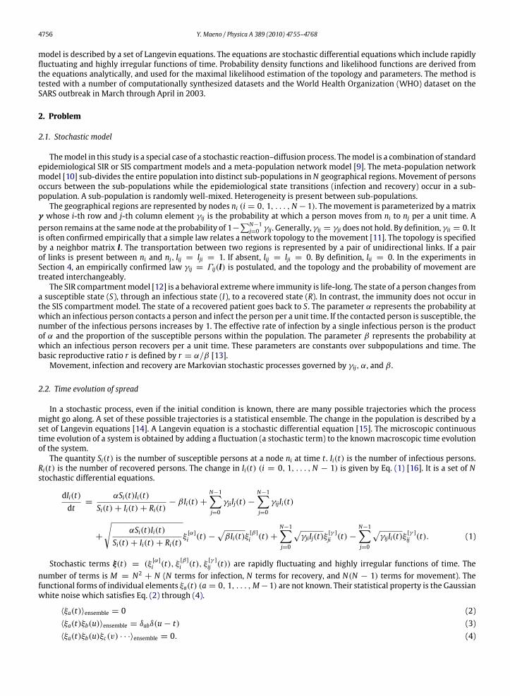
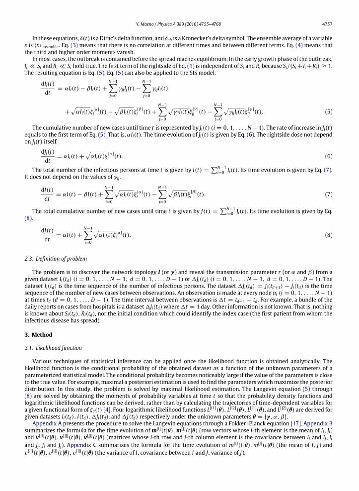
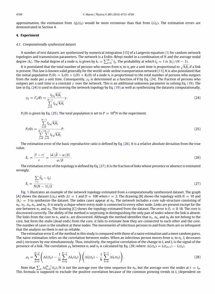
Fig. 1 illustrates an example of the network topology estimated from a computationally synthesized dataset. The graph[A] shows the dataset Ii(td) with 1t = 1 and D = 100 when r = 2. The drawing [B] shows the topology with N = 10 and〈ki〉 = 3 to synthesize the dataset. The index cases appear at n0. The network includes a core sub-structure consisting ofn0, n2, n4, n5, and n9. It is nearly a clique where every node is connected to every other node. Links are present except for theone between n5 and n9. The drawing [C] shows the topology estimated from the dataset. The error is El = 0.18. The core isdiscovered correctly. The ability of themethod is surprising in distinguishing the only pair of nodes where the link is absent.The links from the core to n1 and n7 are discovered. Although the method identifies that n3, n6, and n8 do not belong to thecore, but form the stubs (dead ends) from the core, it fails to estimate how they are connected to each other and the core.The number of cases is the smallest at these nodes. Themovements of infectious persons to and from them are so infrequentthat the analysis on them is not so reliable.The estimation error El of themethod in this study is comparedwith those of a naive estimation and amere randomguess.

The naive estimation relies on the correlation between nodes. When an infectious person moves from ni to nj, Ii decreasesand Ij increases by one simultaneously. Thus, intuitively, the negative correlation of the change in Ii and Ij is the signal of thepresence of a link. The correlation ρij between ni and nj is calculated by Eq. (28) where1Ii(td) = Ii(td+1)− Ii(td).

ρij =

D−2∑d=0

(1Ii(td)−

1N

N−1∑k=0

1Ik(td)

)(1Ij(td)−

1N

N−1∑k=0

1Ik(td)

). (28)

Note that∑k1I

N−1k=0 (td)/N is not the average over the time sequence for nk, but the average over the nodes at t = td.

This formula is supposed to exclude the positive correlation because of the common growing trends in Ii (dependent on

Y. Maeno / Physica A 389 (2010) 4755–4768 4761

Fig. 1. Example of the network topology estimated from a computationally synthesized dataset. [A]: dataset Ii(td) with 1t = 1 and D = 100 when thebasic reproductive ratio is r = 2 (α = 0.067, β = 0.033, γ = 0.1). Individual curves represent the nodes. [B]: random network topology with N = 10and 〈ki〉 = 3 to synthesize the dataset in [A]. The index cases appear at n0 . At t = t99, I2 > I4 > I0 > I5 > I9 > I7 > I1 > I6 > I8 > I3 . [C]: networktopology estimated from the dataset in [A].

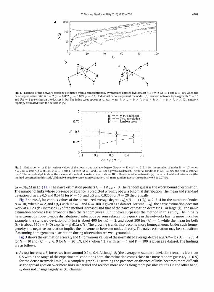
Fig. 2. Estimation error El for various values of the normalized average degree 〈ki〉/(N − 1) (〈ki〉 = 2, 3, 4 for the number of nodes N = 10) whenr = 2 (α = 0.067, β = 0.033, γ = 0.1), and Ii(td)with1t = 1 and D = 100 is given as a dataset. The initial condition is I0(0) = 200 and Ii(0) = 0 for alli 6= 0. The individual plots show the mean and standard deviation over trials for 100 different random networks. [a]: maximal likelihood estimation (themethod presented in this study). [b]: naive negative correlation estimation. [c]: mere random guess (theoretically 0.5± 0.0745).

(α−β)Ii1t in Eq. (11)). The naive estimation predicts lij = 1 if ρij < 0. The random guess is the worst bound of estimation.The number of links whose presence or absence is predicted wrongly obeys a binomial distribution. The mean and standarddeviation of El are 0.5 and 0.0745 for N = 10, and 0.5 and 0.0256 for N = 20 theoretically.Fig. 2 shows El for various values of the normalized average degree 〈ki〉/(N − 1) (〈ki〉 = 2, 3, 4 for the number of nodes

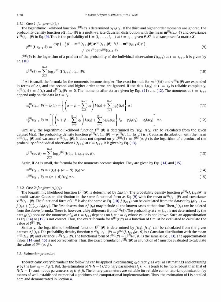
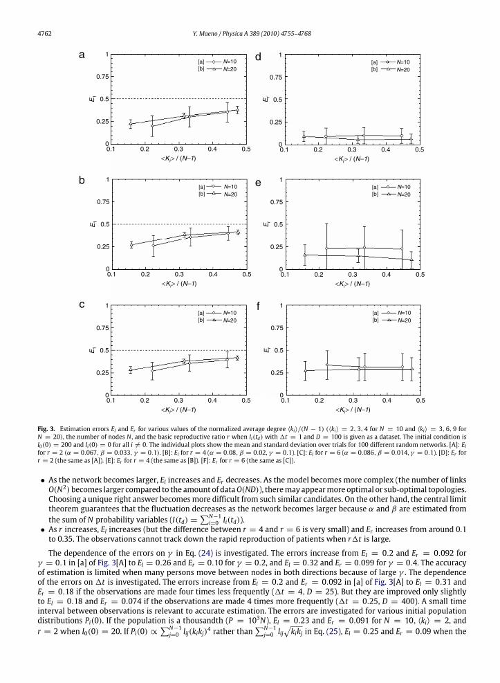
N = 10)when r = 2, and Ii(td)with1t = 1 and D = 100 is given as a dataset. For small 〈ki〉, the naive estimation does notwork at all. As 〈ki〉 increases, El of the method increases and that of the naive estimation decreases. For large 〈ki〉, the naiveestimation becomes less erroneous than the random guess. But, it never surpasses the method in this study. The initiallyheterogeneous node-to-node distribution of infectious persons relaxes more quickly in the networks having more links. Forexample, the standard deviation of Ii(t99) is about 400 for 〈ki〉 = 2, and about 300 for 〈ki〉 = 4, while the mean for both〈ki〉 is about 550 (≈ I0(0) exp((α − β)D1t)/N). The growing trends also become more homogeneous. Under such homo-geneity, the negative correlation implies the movements between nodes directly. The naive estimation may be a substituteif assuming homogeneous distribution during observation are well-grounded.Fig. 3 shows the estimation errors El and Er for various values of the normalized average degree 〈ki〉/(N−1) (〈ki〉 = 2, 3, 4

for N = 10 and 〈ki〉 = 3, 6, 9 for N = 20),N , and r when Ii(td)with1t = 1 and D = 100 is given as a dataset. The findingsare as follows.

• As 〈ki〉 increases, El increases from around 0.2 to 0.4. Although El (the average ± standard deviation) remains less than0.5 within the range of the experimental conditions here, the estimation comes close to a mere random guess (El → 0.5)for the dense network limit (→ a complete graph). Discerning the presence or absence of links becomes more difficultas the spread goes on over more links in parallel and reaches more nodes along more possible routes. On the other hand,Er does not change largely as 〈ki〉 changes.

4762 Y. Maeno / Physica A 389 (2010) 4755–4768

1

0.75

0.5E1

0.25

0

[a][b]

N=10N=20

0.1 0.2 0.3<Ki> / (N–1)

0.4 0.5

1

0.75

0.5E1

0.25

0

[a][b]

N=10N=20

0.1 0.2 0.3<Ki> / (N–1)

0.4 0.5

1

0.75

0.5E1

0.25

0

[a][b]

N=10N=20

0.1 0.2 0.3<Ki> / (N–1)

0.4 0.5

1

0.75

0.5Er

0.25

0

[a][b]

N=10N=20

0.1 0.2 0.3<Ki> / (N–1)

0.4 0.5

1

0.75

0.5Er

0.25

0

[a][b]

N=10N=20

0.1 0.2 0.3<Ki> / (N–1)

0.4 0.5

1

0.75

0.5Er

0.25

0

[a][b]

N=10N=20

0.1 0.2 0.3<Ki> / (N–1)

0.4 0.5

a d

b e

c f

Fig. 3. Estimation errors El and Er for various values of the normalized average degree 〈ki〉/(N − 1) (〈ki〉 = 2, 3, 4 for N = 10 and 〈ki〉 = 3, 6, 9 forN = 20), the number of nodes N , and the basic reproductive ratio r when Ii(td) with 1t = 1 and D = 100 is given as a dataset. The initial condition isI0(0) = 200 and Ii(0) = 0 for all i 6= 0. The individual plots show the mean and standard deviation over trials for 100 different random networks. [A]: Elfor r = 2 (α = 0.067, β = 0.033, γ = 0.1). [B]: El for r = 4 (α = 0.08, β = 0.02, γ = 0.1). [C]: El for r = 6 (α = 0.086, β = 0.014, γ = 0.1). [D]: Er forr = 2 (the same as [A]). [E]: Er for r = 4 (the same as [B]). [F]: Er for r = 6 (the same as [C]).

• As the network becomes larger, El increases and Er decreases. As the model becomes more complex (the number of linksO(N2)becomes larger compared to the amount of dataO(ND)), theremay appearmore optimal or sub-optimal topologies.Choosing a unique right answer becomesmore difficult from such similar candidates. On the other hand, the central limittheorem guarantees that the fluctuation decreases as the network becomes larger because α and β are estimated fromthe sum of N probability variables (I(td) =

∑N−1i=0 Ii(td)).

• As r increases, El increases (but the difference between r = 4 and r = 6 is very small) and Er increases from around 0.1to 0.35. The observations cannot track down the rapid reproduction of patients when r1t is large.

The dependence of the errors on γ in Eq. (24) is investigated. The errors increase from El = 0.2 and Er = 0.092 forγ = 0.1 in [a] of Fig. 3[A] to El = 0.26 and Er = 0.10 for γ = 0.2, and El = 0.32 and Er = 0.099 for γ = 0.4. The accuracyof estimation is limited when many persons move between nodes in both directions because of large γ . The dependenceof the errors on 1t is investigated. The errors increase from El = 0.2 and Er = 0.092 in [a] of Fig. 3[A] to El = 0.31 andEr = 0.18 if the observations are made four times less frequently (1t = 4,D = 25). But they are improved only slightlyto El = 0.18 and Er = 0.074 if the observations are made 4 times more frequently (1t = 0.25, D = 400). A small timeinterval between observations is relevant to accurate estimation. The errors are investigated for various initial populationdistributions Pi(0). If the population is a thousandth (P = 103N), El = 0.23 and Er = 0.091 for N = 10, 〈ki〉 = 2, andr = 2 when I0(0) = 20. If Pi(0) ∝

∑N−1j=0 lij(kikj)

4 rather than∑N−1j=0 lij

√kikj in Eq. (25), El = 0.25 and Er = 0.09 when the

Y. Maeno / Physica A 389 (2010) 4755–4768 4763

Er

[a][b]

N=10N=20

<Ki> / (N–1)

1

0.75

0.5

0.25

00.1 0.2 0.3 0.4 0.5

Er

[a][b]

N=10N=20

<Ki> / (N–1)

1

0.75

0.5

0.25

00.1 0.2 0.3 0.4 0.5

Er

[a][b]

N=10N=20

<Ki> / (N–1)

1

0.75

0.5

0.25

00.1 0.2 0.3 0.4 0.5

E1

[a][b]

N=10N=20

<Ki> / (N–1)

1

0.75

0.5

0.25

00.1 0.2 0.3 0.4 0.5

E1

[a][b]

N=10N=20

<Ki> / (N–1)

1

0.75

0.5

0.25

00.1 0.2 0.3 0.4 0.5

E1

[a][b]

N=10N=20

<Ki> / (N–1)

1

0.75

0.5

0.25

00.1 0.2 0.3 0.4 0.5

a

b

c

d

e

f

Fig. 4. Estimation errors El and Er for various values of 〈ki〉/(N−1),N , and r when1Ji(td)with1t = 1 andD = 100 is given as a dataset. The experimentalconditions are the same as those for Fig. 3.

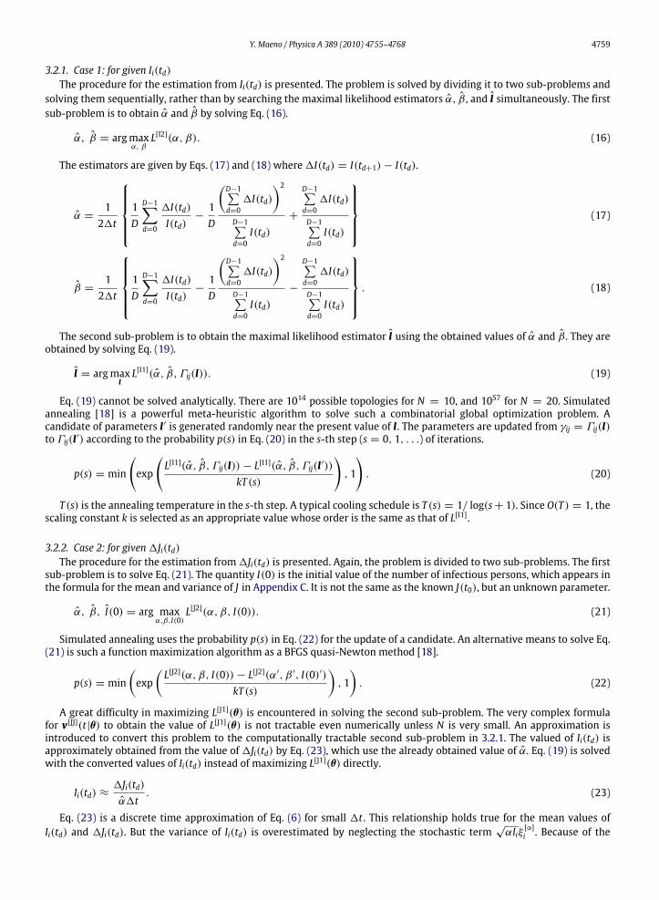
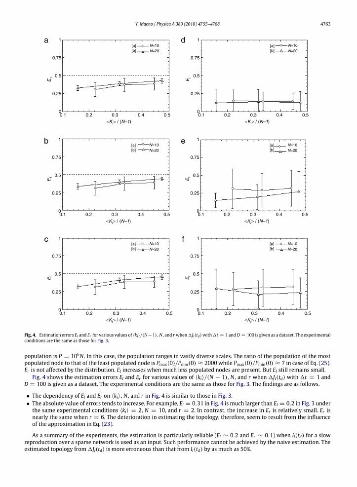
population is P = 106N . In this case, the population ranges in vastly diverse scales. The ratio of the population of the mostpopulated node to that of the least populated node is Pmax(0)/Pmin(0) ≈ 2000 while Pmax(0)/Pmin(0) ≈ 7 in case of Eq. (25).Er is not affected by the distribution. El increases when much less populated nodes are present. But El still remains small.Fig. 4 shows the estimation errors El and Er for various values of 〈ki〉/(N − 1),N , and r when 1Ji(td) with 1t = 1 and

D = 100 is given as a dataset. The experimental conditions are the same as those for Fig. 3. The findings are as follows.

• The dependency of El and Er on 〈ki〉,N , and r in Fig. 4 is similar to those in Fig. 3.• The absolute value of errors tends to increase. For example, El = 0.31 in Fig. 4 is much larger than El = 0.2 in Fig. 3 underthe same experimental conditions 〈ki〉 = 2,N = 10, and r = 2. In contrast, the increase in Er is relatively small. Er isnearly the same when r = 6. The deterioration in estimating the topology, therefore, seem to result from the influenceof the approximation in Eq. (23).

As a summary of the experiments, the estimation is particularly reliable (El ∼ 0.2 and Er ∼ 0.1) when Ii(td) for a slowreproduction over a sparse network is used as an input. Such performance cannot be achieved by the naive estimation. Theestimated topology from1Ji(td) is more erroneous than that from Ii(td) by as much as 50%.

4764 Y. Maeno / Physica A 389 (2010) 4755–4768

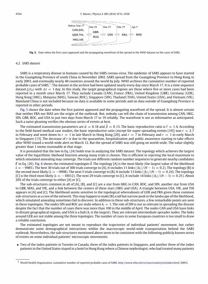
Fig. 5. Date when the first cases appeared and the propagating wavefront of the spread in the WHO dataset on the cases of SARS.

4.2. SARS dataset

SARS is a respiratory disease in humans caused by the SARS corona-virus. The epidemic of SARS appears to have startedin the Guangdong Province of south China in November 2002. SARS spread from the Guangdong Province to Hong Kong inearly 2003, and eventually nearly 40 countries around the world by July. WHO archives the cumulative number of reportedprobable cases of SARS.1. The dataset in the archive had been updated nearly every day since March 17. It is a time sequencedataset Ji(td) with 1t = 1 day. In this study, the target geographical regions are those where five or more cases had beenreported in a month since March 17. They include Canada (CAN), France (FRA), United Kingdom (GBR), Germany (GER),Hong Kong (HKG), Malaysia (MAS), Taiwan (ROC), Singapore (SIN), Thailand (THA), United States (USA), and Vietnam (VIE).Mainland China is not included because no data is available in some periods and no data outside of Guangdong Province isreported in other periods.Fig. 5 shows the date when the first patient appeared and the propagating wavefront of the spread. It is almost certain

that neither FRA nor MAS are the origin of the outbreak. But, nobody can tell the chain of transmission among CAN, HKG,SIN, GBR, ROC, and USA in just two days from March 17 to 19 reliably. The wavefront is not as informative as anticipated.Such a naive gleaning verifies the obvious series of events at best.The estimated transmission parameters are α = 0.18 and β = 0.13. The basic reproductive ratio is r = 1.4. According

to the field-based medical case studies, the basic reproductive ratio (except for super-spreading events [19]) was r = 2.7in February and went down to r = 1 in late March in Hong Kong [20], and r = 7 in February and r = 1 in early Marchin Singapore [13]. The decrease of r is due to the quarantine, hospitalization and public awareness starting to take effectsafter WHO issued a world-wide alert on March 12. But the spread of SARS was still going on world-wide. The value slightlygreater than 1 seems reasonable at that stage.It is postulated that the law in Eq. (24) holds true in analyzing the SARS dataset. The topology which achieves the largest

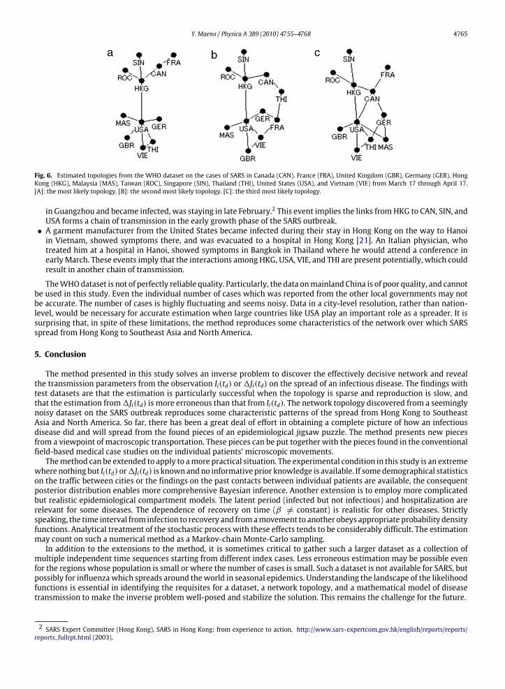
value of the logarithmic likehood function among many trials is chosen. This is efficient in rejecting the local maximum towhich simulated annealingmay converge. The trials use different random number sequences to generate nearby candidatesl ′ in Eq. (20). Fig. 6 shows the estimated topologies l. The topology [A] is the most likely (the largest value of the likelihoodL = −9985). The best 30 trials out of 300 trials converge to [A]. It includes 11 links (〈ki〉/(N − 1) = 0.2). The topology [B] isthe secondmost likely (L = −9998). The next 5 trials converge to [B]. It include 13 links (〈ki〉/(N−1) = 0.24). The topology[C] is the third most likely (L = −10012). The next 29 trials converge to [C]. It include 14 links (〈ki〉/(N − 1) = 0.25). About20% of the trials converge to either [A] or [C].The sub-structures common in all of [A], [B], and [C] are a star from HKG to CAN, ROC, and SIN, another star from USA

to GBR, MAS, and VIE, and a link between the centers of these stars (HKG and USA). A triangle between USA, VIE, and THIappears in [A] and [C]. The likelihood seems sensitive to the topological whereabouts of GER and FRA given these commonsub-structures as a core of the network. Thismayhappen tomake [B] a tall but narrowpeak in the landscape of the likelihood,which simulated annealing sometimes fail to discover. In addition to these sub-structures, a few remarkable points are seenin these topologies. The nodes SIN and ROC are stubs where ki = 1. The role of SIN is not so relevant in spreading the diseasedespite the fact that the number of cases there was more than 100 in the middle of April. The nodes CAN and USA have linksto distant geographical regions, and USA is a hub (ki is the largest). They are relevant intermediate spreader nodes. The linksaround GER are not stable among the three topologies. The number of cases in some European countries is too small to drawa reliable conclusion.The estimated topologies are not meant to reproduce the trajectories of individual patients’ movement, but rather

demonstrate some demographical interactions within the macroscopic world-wide transportation behind the SARSoutbreak. Nevertheless, the sub-structuresmentioned above seem to be consistent with the following publicly known seriesof events on some individual patients’ microscopic movements.

• Two of the index patients in Toronto in Canada, three of the index patients in Singapore, and another three of the indexpatients in theUnited States stayed in a hotel in Hong Kongwhere a Chinese nephrologist, who had treatedmany patients

1 World Health Organization, cumulative number of reported probable cases of SARS, http://www.who.int/csr/sars/country/en/index.html (2003).

Y. Maeno / Physica A 389 (2010) 4755–4768 4765

Fig. 6. Estimated topologies from the WHO dataset on the cases of SARS in Canada (CAN), France (FRA), United Kingdom (GBR), Germany (GER), HongKong (HKG), Malaysia (MAS), Taiwan (ROC), Singapore (SIN), Thailand (THI), United States (USA), and Vietnam (VIE) from March 17 through April 17.[A]: the most likely topology. [B]: the second most likely topology. [C]: the third most likely topology.

in Guangzhou and became infected, was staying in late February.2 This event implies the links fromHKG to CAN, SIN, andUSA forms a chain of transmission in the early growth phase of the SARS outbreak.• A garment manufacturer from the United States became infected during their stay in Hong Kong on the way to Hanoiin Vietnam, showed symptoms there, and was evacuated to a hospital in Hong Kong [21]. An Italian physician, whotreated him at a hospital in Hanoi, showed symptoms in Bangkok in Thailand where he would attend a conference inearly March. These events imply that the interactions among HKG, USA, VIE, and THI are present potentially, which couldresult in another chain of transmission.

TheWHOdataset is not of perfectly reliable quality. Particularly, the data onmainland China is of poor quality, and cannotbe used in this study. Even the individual number of cases which was reported from the other local governments may notbe accurate. The number of cases is highly fluctuating and seems noisy. Data in a city-level resolution, rather than nation-level, would be necessary for accurate estimation when large countries like USA play an important role as a spreader. It issurprising that, in spite of these limitations, the method reproduces some characteristics of the network over which SARSspread from Hong Kong to Southeast Asia and North America.

5. Conclusion

The method presented in this study solves an inverse problem to discover the effectively decisive network and revealthe transmission parameters from the observation Ii(td) or1Ji(td) on the spread of an infectious disease. The findings withtest datasets are that the estimation is particularly successful when the topology is sparse and reproduction is slow, andthat the estimation from1Ji(td) is more erroneous than that from Ii(td). The network topology discovered from a seeminglynoisy dataset on the SARS outbreak reproduces some characteristic patterns of the spread from Hong Kong to SoutheastAsia and North America. So far, there has been a great deal of effort in obtaining a complete picture of how an infectiousdisease did and will spread from the found pieces of an epidemiological jigsaw puzzle. The method presents new piecesfrom a viewpoint of macroscopic transportation. These pieces can be put together with the pieces found in the conventionalfield-based medical case studies on the individual patients’ microscopic movements.Themethod can be extended to apply to amore practical situation. The experimental condition in this study is an extreme

where nothing but Ii(td) or1Ji(td) is knownandno informative prior knowledge is available. If somedemographical statisticson the traffic between cities or the findings on the past contacts between individual patients are available, the consequentposterior distribution enables more comprehensive Bayesian inference. Another extension is to employ more complicatedbut realistic epidemiological compartment models. The latent period (infected but not infectious) and hospitalization arerelevant for some diseases. The dependence of recovery on time (β 6= constant) is realistic for other diseases. Strictlyspeaking, the time interval from infection to recovery and fromamovement to another obeys appropriate probability densityfunctions. Analytical treatment of the stochastic process with these effects tends to be considerably difficult. The estimationmay count on such a numerical method as a Markov-chain Monte-Carlo sampling.In addition to the extensions to the method, it is sometimes critical to gather such a larger dataset as a collection of

multiple independent time sequences starting from different index cases. Less erroneous estimation may be possible evenfor the regions whose population is small or where the number of cases is small. Such a dataset is not available for SARS, butpossibly for influenzawhich spreads around theworld in seasonal epidemics. Understanding the landscape of the likelihoodfunctions is essential in identifying the requisites for a dataset, a network topology, and a mathematical model of diseasetransmission to make the inverse problem well-posed and stabilize the solution. This remains the challenge for the future.

2 SARS Expert Committee (Hong Kong), SARS in Hong Kong: from experience to action, http://www.sars-expertcom.gov.hk/english/reports/reports/reports_fullrpt.html (2003).

4766 Y. Maeno / Physica A 389 (2010) 4755–4768

Appendix A. Probability density function

A generic form of a Langevin equation for multiple time-dependent variables xi(t) is given by Eq. (29). The fluctuationsξa(t) are stochastic terms.

dxi(t)dt= µi(x0(t), . . . , xN−1(t))+

M−1∑a=0

σia(x0(t), . . . , xN−1(t))ξa(t). (29)

Eq. (29) can be solved by deriving the probability density function p(x, t) for probability variables x = (x0, . . . , xN−1) attime t . The time evolution of p(x, t) is given by the Fokker–Planck equation in Eq. (30).

∂p(x, t)∂t

= −

N−1∑i=0

∂

∂xiAi(x)p(x, t)+

12

N−1∑i,j=0

∂2

∂xi∂xjBij(x)p(x, t). (30)

The coefficients Ai and Bij are given by Eqs. (31) and (32).

Ai(x) = µi(x) (31)

Bij(x) =M−1∑a=0

σia(x)σja(x). (32)

Themean (the first order moment) of xi at t is given bymi(t) = 〈xi〉t =∫xip(x, t)dx. The time evolution ofmi(t) is given

by Eq. (33). It is derived by multiplying Eq. (30) by x and partial integration under the condition where p and ∂p/∂x decaymore rapidly than Ai and Bij near the boundary of the domain of x.

dmi(t)dt= 〈Ai(x)〉t . (33)

The covariance (the second order moment) between xi and xj at t is given by vij(t) = 〈xixj〉t − mi(t)mj(t). The timeevolution of vij(t) is given by Eq. (34). Derivation is similar to that for Eq. (33).

dvij(t)dt= 〈Bij(x)〉t + 〈xiAj(x)〉t + 〈Ai(x)xj〉t . (34)

Higher ordermoments can be obtained recursively as a solution of the differential equationswhich include the calculatedlower order moments.

Appendix B. Moments of Ii and Ji

Eq. (35) through (39) are the differential equations for the time evolution of the first and second order moments of Ii andJi. The symbolsm[I](t|θ),m[J](t|θ) are the rowvectorswhose i-th element is themean of Ii, Ji, and v[II](t|θ), v[IJ](t|θ), v[JJ](t|θ)are the N × N matrices whose i-th row and j-th column element is the covariance between Ii and Ij, Ii and Jj, Ji and Jj. Theunknown network topology and transmission parameters are represented by a symbol θ = {γ, α, β}.

dm[I](t|θ)dt

= m[I](t|θ)aT (35)

dm[J](t|θ)dt

= αm[I](t|θ) (36)

dv[II](t|θ)dt

= av[II](t|θ)+ v[II](t|θ)aT + 〈B〉t (37)

dv[IJ](t|θ)dt

= av[IJ](t|θ)+ α(v[II](t|θ)+ c(t)) (38)

dv[JJ](t|θ)dt

= α(v[IJ](t|θ)+ v[IJ](t|θ)T + c(t)). (39)

Y. Maeno / Physica A 389 (2010) 4755–4768 4767

Definitions of the N × N matrices a, B, and c which appear in Eq. (35) through (39) are given by Eq. (40) through (42).

aij =

(α − β −

n−1∑k=0

γik

)δij + γji (40)

Bij =

{(α + β +

N−1∑k=0

γik

)Ii +

N−1∑k=0

γkiIk

}δij − γijIi − γjiIj (41)

cij(t) = δijm[I]i (t|θ). (42)

Eq. (43) through (47) are the solutions. E is a unit matrix.

m[I](t|θ) = I(0) exp(aTt) (43)

m[J](t|θ) = I(0){α(aT)−1 exp(aTt)− α(aT)−1 + E} (44)

v[II](t|θ) =∫ t

0exp(a(t − t ′))〈B〉t ′ exp(aT(t − t ′))dt ′ (45)

v[IJ](t|θ) =∫ t

0α exp(a(t − t ′))(v[II](t ′|θ)+ c(t ′))dt ′ (46)

v[JJ](t|θ) =∫ t

0α(v[IJ](t ′|θ)+ v[IJ](t ′|θ)T + c(t ′)) dt ′

=

∫ t

0α2∫ t ′

0exp(a(t ′ − t ′′))(v[II](t ′′|θ)+ c(t ′′))

+ (v[II](t ′′|θ)+ c(t ′′)) exp(aT(t ′ − t ′′))dt ′′ + αc(t ′) dt ′. (47)

Appendix C. Moments of I and J

Eq. (48) through (52) are the differential equations for the time evolution of the first and second order moments of Iand J . The symbols m[I](t|θ),m[J](t|θ) are the mean of I, J , and v[II](t|θ), v[IJ](t|θ), v[JJ](t|θ) are the variance of I , covariancebetween I and J , variance of J .

dm[I](t|θ)dt

= (α − β)m[I](t|θ) (48)

dm[J](t|θ)dt

= αm[I](t|θ) (49)

dv[II](t|θ)dt

= 2(α − β)v[II](t|θ)+ (α + β)m[I](t|θ) (50)

dv[IJ](t|θ)dt

= (α − β)v[IJ](t|θ)+ α(v[II](t|θ)+m[I](t|θ)) (51)

dv[JJ](t|θ)dt

= α(2v[IJ](t|θ)+m[I](t|θ)). (52)

Eq. (53) through (57) are the solutions.

m[I](t|θ) = I(0) exp(α − β)t (53)

m[J](t|θ) = I(0)(

α

α − βexp(α − β)t −

β

α − β

)(54)

v[II](t|θ) = I(0)α + β

α − β(exp 2(α − β)t − exp(α − β)t) (55)

v[IJ](t|θ) = I(0){α(α + β)

(α − β)2exp 2(α − β)t −

(α(α + β)

(α − β)2+2αβα − β

t)exp(α − β)t

}(56)

v[JJ](t|θ) = I(0)[α2(α + β)

(α − β)3exp 2(α − β)t −

{α(α + β)

(α − β)2+

4α2β(α − β)2

t}exp(α − β)t −

αβ(α + β)

(α − β)3

]. (57)

4768 Y. Maeno / Physica A 389 (2010) 4755–4768

References

[1] D.W. Walker, D. Allingham, H.W.J. Lee, M. Small, Parameter inference in small world network disease models with approximate Bayesiancomputational methods, Physica A 389 (2010) 540–548.

[2] M. Small, C.K. Tse, D.M. Walker, Super-spreaders and the rate of transmission of the SARS virus, Physica D 215 (2006) 146–158.[3] M.J. Keeling, S.P. Brooks, C.A. Gilligan, Using conservation of pattern to estimate spatial parameters from a single snapshot, Proceedings of the NationalAcademy of Sciences USA 101 (2004) 9155–9160.

[4] C.E. Dangerfield, J.V. Ross, M.J. Keeling, Integrating stochasticity and network structure into an epidemic model, Journal of the Royal Society Interface(2009) doi:10.1098/rsif.2008.0410.

[5] S. Riley, Large-scale spatial-transmission models of infectious disease, Science 316 (2007) 1298–1301.[6] Y. Maeno, Node discovery problem for a social network, Connections 29 (2009) 62–76.[7] M.G. Rabbat, M.A.T. Figueiredo, R.D. Nowak, Network inference from co-occurrences, IEEE Transactions on Information Theory 54 (2008) 4053–4068.[8] A. Baronchelli, M. Catanzaro, R. Pastor-Satorras, Bosonic reaction–diffusion processes on scale-free networks, Physical Review E 78 (2008) 01611.[9] M. Simões, M.M.T. da Gama, A. Nunes, Stochastic fluctuations in epidemics on networks, Journal of the Royal Society Interface 5 (2008) 555–566.[10] V. Colizza, A. Vespignani, Invasion threshold in heterogeneous meta-population networks, Physical Review Letters 99 (2007) 148701.[11] A. Barrat, M. Barthélemy, R. Pastor-Satorras, A. Vespignani, The architecture of complex weighted networks, Proceedings of the National Academy of

Sciences USA 101 (2004) 3747–3752.[12] M.J. Keeling, J.V. Ross, On methods for studying stochastic disease dynamics, Journal of the Royal Society Interface 5 (2008) 171–181.[13] M. Lipsitch, et al., Transmission dynamics and control of severe acute respiratory syndrome, Science 300 (2003) 1966–1970.[14] L. Hufnagel, D. Brockmann, T. Geisel, Forecast and control of epidemics in a globalized world, Proceedings of the National Academy of Sciences USA

101 (2004) 15124–15129.[15] P.E. Kloeden, E. Platen, Numerical Solution of Stochastic Differential Equations, Springer, 1992.[16] V. Colizza, A. Barret, M. Barthélemy, A. Vespignani, The role of the airline transportation network in the prediction and predictability of global

epidemics, Proceedings of the National Academy of Sciences USA 103 (2006) 2015–2020.[17] N.G. van Kampen, Stochastic Processes in Physics and Chemistry, Elsevier, 2007.[18] W.H. Press, S.A. Teukolsky, W.T. Vetterling, B.P. Flannery, Numerical Recipes: The Art of Scientific Computing, Cambridge University Press, 2007.[19] R. Fujie, T. Odagaki, Effects of superspreaders in spread of epidemic, Physica A 374 (2007) 843–852.[20] S. Riley, et al., Transmission dynamics of the etiological agent of SARS in Hong Kong: impact of public health interventions, Science 300 (2003)

1961–1966.[21] K.T. Greenfeld, China Syndrome, HarperCollins Publishers, 2006.