Embed Size (px)
Citation preview

Discovering and Summarizing Email Conversations
by
Xiaodong Zhou
B.Eng., Dalian Maritime University, 1996M.Eng., Tsinghua University , 1999
M.Sc., The University of British Columbia, 2003
A THESIS SUBMITTED IN PARTIAL FULFILMENT OFTHE REQUIREMENTS FOR THE DEGREE OF
Doctor of Philosophy
in
The Faculty of Graduate Studies
(Computer Science)
The University Of British Columbia
(Vancouver)
February 2008
c© Xiaodong Zhou 2008

ii
Abstract
With the ever increasing popularity of emails, it is very common nowadays thatpeople discuss specific issues, events or tasks among a group of people by emails.Those discussions can be viewed as conversations via emails and are valuablefor the user as a personal information repository. For instance, in 10 minutesbefore a meeting, a user may want to quickly go through a previous discussionvia emails that is going to be discussed in the meeting soon. In this case, ratherthan reading each individual email one by one, it is preferable to read a concisesummary of the previous discussion with major information summarized. Inthis thesis, we study the problem of discovering and summarizing email conver-sations. We believe that our work can greatly support users with their emailfolders.
However, the characteristics of email conversations, e.g., lack of synchro-nization, conversational structure and informal writing style, make this taskparticularly challenging. In this thesis, we tackle this task by considering thefollowing aspects: discovering emails in one conversation, capturing the conver-sation structure and summarizing the email conversation. We first study howto discover all emails belonging to one conversation. Specifically, we study thehidden email problem, which is important for email summarization and otherapplications but has not been studied before. We propose a framework to dis-cover and regenerate hidden emails. The empirical evaluation shows that thisframework is accurate and scalable to large folders.
Second, we build a fragment quotation graph to capture email conversa-tions. The hidden emails belonging to each conversation are also included intothe corresponding graph. Based on the quotation graph, we develop a novelemail conversation summarizer, ClueWordSummarizer. The comparison witha state-of-the-art email summarizer as well as with a popular multi-documentsummarizer shows that ClueWordSummarizer obtains a higher accuracy in mostcases.
Furthermore, to address the characteristics of email conversations, we studyseveral ways to improve the ClueWordSummarizer by considering more lexicalfeatures. The experiments show that many of those improvements can signifi-cantly increase the accuracy especially the subjective words and phrases.

iii
Contents
Abstract . . . . . . . . . . . . . . . . . . . . . . . . . . . . . . . . . . . . ii
Contents . . . . . . . . . . . . . . . . . . . . . . . . . . . . . . . . . . . . iii
List of Tables . . . . . . . . . . . . . . . . . . . . . . . . . . . . . . . . . vi
List of Figures . . . . . . . . . . . . . . . . . . . . . . . . . . . . . . . . vii
Acknowledgements . . . . . . . . . . . . . . . . . . . . . . . . . . . . . ix
1 Introduction . . . . . . . . . . . . . . . . . . . . . . . . . . . . . . . 1
2 Related Work . . . . . . . . . . . . . . . . . . . . . . . . . . . . . . . 62.1 Multi-Document Summarization . . . . . . . . . . . . . . . . . . 62.2 Email Summarization . . . . . . . . . . . . . . . . . . . . . . . . 72.3 Newsgroup Summarization . . . . . . . . . . . . . . . . . . . . . 102.4 Email Management . . . . . . . . . . . . . . . . . . . . . . . . . . 112.5 Subjective Opinion Mining . . . . . . . . . . . . . . . . . . . . . 112.6 Evaluation Metrics . . . . . . . . . . . . . . . . . . . . . . . . . . 122.7 Searching for Similar Documents . . . . . . . . . . . . . . . . . . 14
3 Discovering and Regenerating Hidden Emails . . . . . . . . . . 153.1 Introduction . . . . . . . . . . . . . . . . . . . . . . . . . . . . . . 153.2 Identifying Hidden Fragments . . . . . . . . . . . . . . . . . . . . 163.3 Creating The Precedence Graph . . . . . . . . . . . . . . . . . . 173.4 The Bulletized Email Model . . . . . . . . . . . . . . . . . . . . . 183.5 A Necessary and Sufficient Condition . . . . . . . . . . . . . . . . 223.6 Regeneration Algorithms . . . . . . . . . . . . . . . . . . . . . . . 24
3.6.1 Algorithm for Strict and Complete Parent-child Graph . . 243.6.2 Heuristics Dealing with Non-strictness and Incompleteness 27
3.7 Summary . . . . . . . . . . . . . . . . . . . . . . . . . . . . . . . 30
4 Optimizations for Hidden Email Discovery and Regeneration 314.1 Introduction . . . . . . . . . . . . . . . . . . . . . . . . . . . . . . 314.2 HiddenEmailFinder: An Overall Framework . . . . . . . . . . . . 324.3 Email Filtration by Word Indexing . . . . . . . . . . . . . . . . . 33
4.3.1 Word-based Filtration: A Basic Approach . . . . . . . . . 33

Contents iv
4.3.2 Enhanced Filtration with Segments . . . . . . . . . . . . . 344.3.3 Enhanced Filtration with Sliding Windows . . . . . . . . 37
4.4 LCS-Anchoring by Indexing . . . . . . . . . . . . . . . . . . . . . 374.5 Empirical Evaluation . . . . . . . . . . . . . . . . . . . . . . . . . 38
4.5.1 The Enron Email Dataset . . . . . . . . . . . . . . . . . . 384.5.2 Prevalence of Emails Containing Hidden Fragments . . . 394.5.3 Accuracy Evaluation . . . . . . . . . . . . . . . . . . . . . 424.5.4 Word-based Email Filtration and LCS-Anchoring . . . . . 454.5.5 Email Filtration by Sliding Windows . . . . . . . . . . . . 484.5.6 Scalability . . . . . . . . . . . . . . . . . . . . . . . . . . . 48
4.6 Summary . . . . . . . . . . . . . . . . . . . . . . . . . . . . . . . 53
5 Summarizing Email Conversations with Clue Words . . . . . . 545.1 Introduction . . . . . . . . . . . . . . . . . . . . . . . . . . . . . . 545.2 Building the Fragment Quotation Graph . . . . . . . . . . . . . . 55
5.2.1 Identifying Quoted and New Fragments . . . . . . . . . . 555.2.2 Creating Nodes . . . . . . . . . . . . . . . . . . . . . . . . 555.2.3 Creating Edges . . . . . . . . . . . . . . . . . . . . . . . . 57
5.3 Email Summarization Methods . . . . . . . . . . . . . . . . . . . 585.3.1 Clue Words . . . . . . . . . . . . . . . . . . . . . . . . . . 585.3.2 Algorithm CWS . . . . . . . . . . . . . . . . . . . . . . . 595.3.3 MEAD: A Centroid-based Multi-document Summarizer . 615.3.4 Summarization Using RIPPER . . . . . . . . . . . . . . . 61
5.4 Result 1: User Study . . . . . . . . . . . . . . . . . . . . . . . . . 625.4.1 Dataset Setup . . . . . . . . . . . . . . . . . . . . . . . . . 635.4.2 Result of the User Study . . . . . . . . . . . . . . . . . . 63
5.5 Result 2: Empirical Evaluation of CWS . . . . . . . . . . . . . . 655.5.1 Evaluation Metrics . . . . . . . . . . . . . . . . . . . . . . 665.5.2 Comparing CWS with MEAD and RIPPER . . . . . . . . 675.5.3 Comparing CWS with MEAD . . . . . . . . . . . . . . . . 695.5.4 Effectiveness of the Fragment Quotation Graph . . . . . . 71
5.6 Summary . . . . . . . . . . . . . . . . . . . . . . . . . . . . . . . 72
6 Summarization with Lexical Features . . . . . . . . . . . . . . . 736.1 Introduction . . . . . . . . . . . . . . . . . . . . . . . . . . . . . . 736.2 Building the Sentence Quotation Graph . . . . . . . . . . . . . . 74
6.2.1 Create the nodes and edges . . . . . . . . . . . . . . . . . 746.2.2 Measuring the Cohesion Between Sentences . . . . . . . . 75
6.3 Summarization Approaches Based on the Sentence QuotationGraph . . . . . . . . . . . . . . . . . . . . . . . . . . . . . . . . . 80
6.4 Summarization with Lexical Cues . . . . . . . . . . . . . . . . . . 836.4.1 Cue Phrases . . . . . . . . . . . . . . . . . . . . . . . . . . 836.4.2 Subjective Opinion . . . . . . . . . . . . . . . . . . . . . . 856.4.3 Roget’s Thesaurus . . . . . . . . . . . . . . . . . . . . . . 866.4.4 Measure Sentence Importance by Lexical Cues . . . . . . 86
6.5 Empirical Evaluation . . . . . . . . . . . . . . . . . . . . . . . . . 88

Contents v
6.5.1 Evaluating the Weight of Edges . . . . . . . . . . . . . . . 886.5.2 Evaluating Sentence-based Lexical Cues . . . . . . . . . . 906.5.3 Reevaluation with a New Dataset . . . . . . . . . . . . . . 100
6.6 Summary . . . . . . . . . . . . . . . . . . . . . . . . . . . . . . . 107
7 Conclusions and Future Work . . . . . . . . . . . . . . . . . . . . 1097.1 Conclusions . . . . . . . . . . . . . . . . . . . . . . . . . . . . . . 1097.2 Future Work . . . . . . . . . . . . . . . . . . . . . . . . . . . . . 110
Bibliography . . . . . . . . . . . . . . . . . . . . . . . . . . . . . . . . . 112
A Proof of Theorem 1 . . . . . . . . . . . . . . . . . . . . . . . . . . . 120
B Evaluating Regeneration Heuristics on a Synthetic Dataset . 125
C PageRank for Email Summarization . . . . . . . . . . . . . . . . 128C.1 PageRank for Summarization . . . . . . . . . . . . . . . . . . . . 128C.2 Empirical Evaluation . . . . . . . . . . . . . . . . . . . . . . . . . 129

vi
List of Tables
4.1 Percentage of Root Mapping Types . . . . . . . . . . . . . . . . . 444.2 Percentage of Different Types w.r.t. minLen on Uncleansed
Dataset . . . . . . . . . . . . . . . . . . . . . . . . . . . . . . . . 44
5.1 GSValues and Possible Selections for Overall Essential Sentences 645.2 Precision of RIPPER, CWS and MEAD . . . . . . . . . . . . . . 68
6.1 Aggregated Precision and P-value for Communication Words . . 956.2 Compare Dataset 1 and Dataset 2 . . . . . . . . . . . . . . . . . 1016.3 Aggregate Pyramid Precision for MergedDataset . . . . . . . . . 1026.4 ROUGE Evaluation for MergedDataset . . . . . . . . . . . . . . 1046.5 Dataset 2: Aggregated Precision over Various Summary Length
and P-value . . . . . . . . . . . . . . . . . . . . . . . . . . . . . . 1066.6 Integrate CWS with Lexical Cues in MergedDataset . . . . . . . 1086.7 Integrate MEAD with Lexical Cues in MergedDataset . . . . . . 108

vii
List of Figures
3.1 Case Study - the Missing/Hidden Email . . . . . . . . . . . . . . 193.2 Case Study - Emails in the Folder . . . . . . . . . . . . . . . . . 193.3 The Precedence Graph . . . . . . . . . . . . . . . . . . . . . . . . 203.4 Example of Precedence Graphs and Bulletized Emails . . . . . . 213.5 Examples of Parent-Child Subgraph . . . . . . . . . . . . . . . . 223.6 Examples Illustrating Strictness . . . . . . . . . . . . . . . . . . . 233.7 Examples Illustrating Incompleteness . . . . . . . . . . . . . . . . 243.8 A Skeleton of Algorithm graph2email . . . . . . . . . . . . . . . . 263.9 An Example Illustrating Algorithm graph2email . . . . . . . . . 273.10 Edge Removal for Completeness . . . . . . . . . . . . . . . . . . . 283.11 A Skeleton of Algorithm Star-cut . . . . . . . . . . . . . . . . . . 29
4.1 A Skeleton of Algorithm HiddenEmailFinder . . . . . . . . . . . 334.2 A Skeleton of Algorithm EmailFiltration(word-based) . . . . . . 344.3 A Skeleton of Algorithm EmailFiltration(segment-based) . . . . . 354.4 Proof of Segmentation Upperbound . . . . . . . . . . . . . . . . . 364.5 A Skeleton of Algorithm LCS-Anchoring . . . . . . . . . . . . . . 394.6 Emails Containing Hidden Fragments . . . . . . . . . . . . . . . 404.7 Histogram of Recollection Rates . . . . . . . . . . . . . . . . . . 414.8 Example of Mapping Between Roots and Regenerated Hidden
Emails . . . . . . . . . . . . . . . . . . . . . . . . . . . . . . . . . 434.9 Type of Overlapping w.r.t. minLen . . . . . . . . . . . . . . . . 454.10 Effectiveness of Optimizations . . . . . . . . . . . . . . . . . . . . 474.11 Email Filtration Based on Sliding Windows . . . . . . . . . . . . 494.12 Runtime to Identify Hidden Fragments . . . . . . . . . . . . . . . 504.13 Runtime to Identify Hidden Fragments of 10 Individual Folders . 504.14 Scalability w.r.t. ft . . . . . . . . . . . . . . . . . . . . . . . . . . 52
5.1 A Real Example . . . . . . . . . . . . . . . . . . . . . . . . . . . 565.2 Example of Clue Words . . . . . . . . . . . . . . . . . . . . . . . 595.3 Algorithm CWS . . . . . . . . . . . . . . . . . . . . . . . . . . . 605.4 Features Used by RIPPER . . . . . . . . . . . . . . . . . . . . . 625.5 Ratio of ClueScore of Overall Essential Sentences and the Re-
maining Ones . . . . . . . . . . . . . . . . . . . . . . . . . . . . . 655.6 Distribution of GSValue . . . . . . . . . . . . . . . . . . . . . . . 665.7 Accuracy of CWS and MEAD . . . . . . . . . . . . . . . . . . . . 70

List of Figures viii
5.8 Pyramid Precision of CWS and Two Random Alternatives . . . . 71
6.1 Algorithm to Generate the Sentence Quotation Graph . . . . . . 756.2 Create the Sentence Quotation Graph from the Fragment Quo-
tation Graph . . . . . . . . . . . . . . . . . . . . . . . . . . . . . 766.3 An Example of Clue Words in the Sentence Quotation Graph . . 786.4 Heuristic to Use Semantic Similarity Based on the WordNet . . . 796.5 Example of Lexical Cues . . . . . . . . . . . . . . . . . . . . . . . 846.6 Communication of Ideas in Roget’s Thesaurus . . . . . . . . . . . 876.7 Accuracy of Using Cosine Similarity . . . . . . . . . . . . . . . . 896.8 Evaluating the Cue Phrases . . . . . . . . . . . . . . . . . . . . . 926.9 Evaluating the Subjective Words in OpFind . . . . . . . . . . . . 936.10 Evaluating the Appraisal Words . . . . . . . . . . . . . . . . . . . 946.11 Evaluating the List of OpBear . . . . . . . . . . . . . . . . . . . . 966.12 Evaluating the ComVerb . . . . . . . . . . . . . . . . . . . . . . . 976.13 Evaluating the ComNoun . . . . . . . . . . . . . . . . . . . . . . 986.14 Evaluating the ComAdjv . . . . . . . . . . . . . . . . . . . . . . . 996.15 Evaluating the ComAll . . . . . . . . . . . . . . . . . . . . . . . . 1006.16 Compare MEAD and CWS in Dataset 2 . . . . . . . . . . . . . . 1036.17 Compare CWS and MEAD in Dataset 1 and 2 . . . . . . . . . . 1046.18 Dataset 2: Compare CWS, CWS-WordNet and CWS-Cosine . . 105
A.1 Proof for Sufficiency . . . . . . . . . . . . . . . . . . . . . . . . . 120A.2 Formation of V and U . . . . . . . . . . . . . . . . . . . . . . . . 121A.3 Adding Nodes into dG′ . . . . . . . . . . . . . . . . . . . . . . . . 122A.4 Proof for Necessity . . . . . . . . . . . . . . . . . . . . . . . . . . 124
B.1 Scalability with Respect to Folder Size and Quotation Length . . 127
C.1 PageRank vs. CWS with Different Edge Weight . . . . . . . . . . 131

ix
Acknowledgements
I am deeply indebted with my supervisors Dr. Raymond T. Ng and Dr. GiuseppeCarenini, who lead me through the long journey of the Doctoral program. Notonly did they give me excellent advice but also gave me enough time and spaceto think, understand and practice by myself. I will never forget the encourage-ment they gave me when I met with various obstacles and difficulties. Withouttheir guidance and help, this thesis will never be possible.
I would like to thank my supervision committee member, Dr. Laks V.S.Lakshmanan, for inspiration and valuable feedbacks for my research. I wouldalso like to thank Dr. Norm Hutchinson and Dr. Hasan Cavusoglu to be myuniversity examiner and Dr. Hosagrahar V. Jagadish to be external examiner.Their comments are valuable to make this thesis better.
I would like to thank Dr. Rachel Pottinger for her help in the past few years.I also owe thanks to all members in the Data Management and Mining Lab, fortheir friendship and encouragement. I also need to thank many of my friendswho accompanied me through the special 5 years in my life, to name a few,Xiushan Feng, Jian Chen, Hui Wang and Shaofeng Bu.
I would like to thank my parents, for their love and support. Those are themost valuable assets I possess. Their love is the light in the sky that alwayscovers me and encourages me to proceed further. A special thank-you goesto my wife, Xiaoyan, for her sacrifice and support. I also owe thanks to mydaughter Linjia. Her smiles took away the clouds in the sky. The duty shebrought to me made me grow together with her.
Finally, I am grateful to people who denounced me, who made me stumbleand even those who hurt me, for they have increased my insights and determi-nation. I would like to thank all people who make me firm and resolute.

1
Chapter 1
Introduction
With the ever increasing popularity of emails, it is very common nowadaysthat people discuss specific issues, events or tasks among a group of people byemails[22][79][15]. Those discussions can be viewed as conversations via emailsand are valuable for the user as a personal information repository[15]. Accordingto one study, about 60% of emails belong to conversations[34].
In this thesis, we study the problem of discovering and summarizing emailconversations. We believe that our work can greatly support users with theiremail folders. For instance, in 10 minutes before a meeting, a user may want toquickly go through a previous discussion via emails about an issue that is goingto be discussed soon. In this case, rather than reading each individual emailone by one, it is preferable to read a concise summary of the previous discussionwith major information summarized. Additionally, when a new email arrives, asummary of the previous related emails can also help users track the discussionand understand the new message in the conversational context. Email summa-rization is also valuable for users reading emails on mobile devices. Given thesmall screen size of handheld devices, it is inconvenient to handle emails in thosedevices. Efforts have been made to re-design the user interface[8]. However, webelieve that providing a concise summary may be just as important[31].
It is critical that the summary is faithful to the original messages. We chooseto select sentences from the original emails and use them as the summary ofthe conversation. Hence, in this thesis, the problem we are studying can bestated as follows: Give a folder of emails MF , discover all email conversationsin MF and generate a summary for each conversation by extracting importantsentences.
However, discovering and summarizing email conversations is a challengingtask. The difficulties can be viewed at least from the following two aspects.
• First, the discovery of an email conversation is difficult. Emails are asyn-chronous conversations which may span over days and even weeks withmany participants, many of whom may just join the discussion in themiddle. How to accurately identify all emails involved in one conversa-tion and extract the corresponding conversation structure is a challengingproblem. This problem has not been well studied so far.
• Second, summarization of email conversations is also difficult. Althoughemail summarization can be viewed as a special case of the general multi-document summarization(MDS), email conversations have their own char-acteristics, e.g., the conversation structure, multiple authors and an infor-

Chapter 1. Introduction 2
mal writing style. Directly applying the existing MDS approaches mayneglect those characteristics and therefore not work well for email conver-sations.
Specifically, in the following we analyze three major challenges for discover-ing and summarizing email conversations. We can see that those three challengesoriginate from the characteristics of emails.
• Regenerating hidden emails is a special challenge for summarizing emailconversations. A hidden email is an email quoted by at least one exist-ing email in a folder, but is not present itself in the same folder. Hiddenemails can occur in many situations. We all have experience of manu-ally shunting emails among folders, making decisions on which emails todelete and which to keep. It often happens that some emails are deleted(un)intentionally, but later on we want to read them again. Forwardedemails are another source of hidden emails. In addition to deleted andforwarded emails, a user may join a discussion in the middle, and hencethe emails she receives may contain previous messages which have neverbeen sent to her directly. Whether the original emails are deleted or neverreceived, they can be found in the quotations of the existing emails. Thehidden email problem is a special characteristic in email conversations andhas not been studied before. In the literature, [14] and [48] mentioned theexistence of some orphaned quotations but they did not study this problemfurther.
To summarize an email conversation, we need to collect all emails involvedin this conversation. For this purpose, hidden emails are as importantas emails explicitly occurring in the folder because they may also carrysome crucial information that need to be included in the summary. Ourexperiment with the Enron dataset shows that 18% important sentences(evaluated by human reviewers) are from hidden emails.
• Extracting the email conversation structure is another challenge for sum-marizing email conversations. Since email conversations are asynchronous,a conversation can span over days or weeks with some participants joiningin the middle. Moreover, one reply may selectively comment on severalparts of a previous email. For example, a quotation can be split into dif-ferent fragments by the new messages, each of which comments on thecorresponding fragment. We call this selective quotation.
To the best of our knowledge, all existing methods dealing with email con-versations use the so called email thread as a representation of the emailconversation structure. The email thread is a hierarchy constructed fromthe email headers, e.g., “Subject”, “Message-id” and “In-reply-to”[37].Each node in this hierarchy corresponds to one email. Conceptually, theheader of an email only records some attributes of this email, but a con-versation is based on the content, i.e., the message in the email body, notthe header. For many applications, email thread is not accurate, becausenot every email software follows the same rule to generate the header[37]

Chapter 1. Introduction 3
[30]. The user may also modify the subject of an reply, in which case thisemail will be separated from the conversation by many existing threadingmethods. More importantly, the current email threading approach canonly extract and represent the email conversation in the email level. Itcannot represent the conversation at a finer granularity, e.g., the level ofselective quotations.
• Summarizing email conversations is also challenging because of the con-versational nature, informal writing style and multiple participants. Theconversation structure is an important characteristic of email conversa-tions that distinguishes them from other documents. How to include theconversation structure in the summarization algorithm is a new topic thathas not been well studied. Most existing email summarization approachesjust use quantitative features to describe the conversation structure, e.g.,the number of replies to an email and the distance to the root in an emailthread[57]. Then, some general MDS methods are applied to summarizethose conversations in a similar way for general document summarization[14][77]. Although such methods consider the conversation structure some-how, they simplify the conversation structure into a few features and donot fully utilize the conversation structure into the summarization proce-dure. How to make use of the conversation structure effectively for emailsummarization is still an unsolved problem.
Other than the conversation structure, email conversations usually involvemultiple participants. We cannot assume that all authors are well-trainedwriters such as columnists for newspapers or university faculties. As aresult, we cannot expect a consistent writing style. Moreover, in manycases, email is an informal way of communication that is different fromthe formal published documents. These characteristics bring in challengesfor summarizing email conversations, where general MDS approaches maynot work well.
Consequently, in this thesis, we propose to solve those three problems in thecorresponding three aspects: regenerating hidden emails, extracting the conver-sation structure and summarizing the email conversation. In the following, webriefly introduce the major contributions of this thesis with respect to thosethree aspects.
• In Chapter 3, we propose a method to discover and regenerate hiddenemails. Ideally, the hidden email can be reconstructed in full and rep-resented exactly as it was first written, i.e., a total order representation.However, doing so will often not be possible. Parts of the original maynot have been quoted in subsequent emails. Even if the entire text doesexist scattered among the various quotations, some uncertainty about thecorrect ordering may remain. In these cases, it is still desirable to settle fora partial order representation, while maintaining utility. Thus, we intro-duce a bulletized model of a reconstructed email that accounts for partial

Chapter 1. Introduction 4
ordering. The email is built from a precedence graph which represents therelative orders among email fragments. The key technical result is a neces-sary and sufficient condition for each component of the precedence graphto be represented as a single bulletized email. Moreover, we develop analgorithm to generate the bulletized email, if the necessary and sufficientcondition is met. We also develop heuristics for generating the emails ifthe graph fails the condition. This framework is useful not only for hid-den email regeneration, but also for the general document forensics wheredifferent document fragments need to be pieced together to reconstructthe original document.
• Although our methods in Chapter 3 deliver the functionality, it cannotdeliver the efficiency, nor the robustness, to deal with large real fold-ers. In Chapter 4, we develop two optimization approaches to improvethe runtime performance of our framework to regenerate hidden emailswithout affecting its accuracy. Both approaches are based on word index-ing(inverted index) and sliding windows. Our results show that hiddenemails are prevalent in the Enron dataset and our framework is accuratein reconstructing hidden emails. The optimization approaches effectivelyimprove the runtime performance over the basic approach by an order ofmagnitude without affecting the accuracy.
• In Chapter 5, we first build a fragment quotation graph to capture emailconversations. Instead of using the header of emails, the fragment quo-tation graph is built by analyzing the quotations embedded in emails.Moreover, the fragment quotation graph provides a fine representation ofthe structure of a conversation. This graph also contains all hidden emailsbelonging to this conversation.
With the fragment quotation graph, we propose an email summarizationmethod, called ClueWordSummarizer (CWS). CWS extracts sentencesfrom an email conversation and uses it as the summary. We compare CWSwith one existing email summarization approach and one generic multi-document summarization approach. The empirical evaluation shows thatCWS has the highest accuracy. In addition, both the fragment quotationgraph and the clue words are valuable for summarizing email conversa-tions.
• In Chapter 6, we try to improve CWS from several aspects. First, weextend the fragment quotation graph into a sentence quotation graph,which can represent the email conversation in the sentence granularity.Second, we extend the concept of clue words from stemming to semanticsimilar words such as synonyms and antonyms. We use the well-knownlexical database WordNet to compute the similarity between two words.Third, we study some sentence-based lexical features, e.g., cue phrasesand subjective words and phrases. The empirical evaluation shows thatsubjective words and phrases can significantly improve the accuracy ofCWS.

Chapter 1. Introduction 5
To summarize, this thesis is organized as follows. In Chapter 2, we discussthe related work. While we develop a framework to discover and regeneratehidden emails in Chapter 3, we develop optimization methods to improve itsruntime performance in Chapter 4. In Chapter 5, we build a fragment quotationgraph to represent the conversation structure and develop a novel summarizationalgorithm ClueWordSummarizer(CWS) that is based on the fragment quotationgraph. In Chapter 6, we try to further improve CWS from many aspects. Weconclude this thesis and propose several directions for future work in Chapter7.

6
Chapter 2
Related Work
Email conversations summarization is a special topic of the general multi-documentsummarization(MDS). In this chapter, we start with the general multi-documentsummarization approaches. Then, we introduce some recent work on emailsummarization. We can see that many of them borrow ideas from the MDSapproaches. We also introduce some work on email management, e.g., emailcleaning and visualization. They study emails from other perspectives and areuseful for email summarization as well. In addition, we also discuss some recentstudies in subjective opinion mining and their applications in summarization.At last, we introduce some popular evaluation metrics for document summa-rization.
2.1 Multi-Document Summarization
Multi-Document Summarization has been studied since 1950’s [40][41]. Ed-mundson et al. [17] gave a survey on the major approaches at that time. Re-cently, with the popularity of Internet and voluminous on-line documents suchas web pages, blogs and on-line discussions, many MDS approaches have beendeveloped within the past few years[3] [55][26][35] [18] [82]. Based on the sum-mary that a MDS system produces, MDS approaches can be divided into twocategories: the extractive summarizer and the abstractive summarizer[41]. Theextractive summarizers pick text units, usually sentences, from the original doc-ument set, and use them as the summary, e.g., MEAD by Radev et al.[55][56],Maximum Marginal Relevance by Goldstein et al.[25][26] and DEMS by Schiff-man et al.[64] Unlike the extractive summarizers which directly select sentencesfrom the original documents as the summary, abstractive summarizers generatenew sentences as the summary by analyzing the existing documents, e.g., Multi-Gen by McKeown et al.[45][43] , RIPTIDES by White et al.[78] and GEA byCarenini et al.[5][4]. In this thesis, the summarization methods we propose areextractive approaches, which select sentences from an email conversation as thesummary. In particular, we use the MEAD system, which is also an extractivesummarizer, as a comparison to our approaches in our empirical evaluation inthe following chapters. Moreover, we can see in the later sections that manyexisting email summarization methods borrow ideas from MEAD.
The MEAD system developed by Radev et al.[56] provides a framework formulti-document summarization. The input to MEAD is a cluster of documentsD and a compression rate r. The output is a summary containing r ∗ D sen-

Chapter 2. Related Work 7
tences from input documents D. MEAD uses a centroid to represent the inputdocuments. The centroid is a vector of words’ average TFIDF values of theinput documents. A word is selected into the centroid if its TFIDF value isgreater than a threshold. Let m denote the total number of words in the cen-troid. Intuitively, the words in the centroid construct a m−dimensional space,in which each input document can be viewed as a point and the centroid is apseudo-document in the center of the input points(documents).
With the centroid representing the “center” of the input documents, MEADcomputes a score for each sentence to represent its salience, and the top r ∗ Dsentences are selected into the summary. The score of s is determined by fourfactors: similarity to the centroid(centroid value), similarity to the first sen-tence in the document(first sentence overlap), position in the document(positionvalue), and redundancy penalty. Suppose sentence si is in document Dk. Thescore of the sentence si is the linear combination of the four values above.
SCORE(si) = (wc ∗ Ci + wf ∗ Fi + wp ∗ Pi − wr ∗ Ri) (2.1)
Ci denotes the similarity between the sentence si and the centroid. It iscomputed by summing up the TFIDF values of all shared words between sand those constructing the centroid. Fi denotes the similarity between thesentence si and the first sentence sk of the document Dk. The similarity ismeasured by the normalized dot product of two sentences’ vector. Pi denotesthe position value of si in document Dk. MEAD assumes that the earlier asentence appears, the more important it is and the higher is the score assignedto it. Ri is redundancy factor that measures the similarity of si to sentenceswith a higher score. At a result, MEAD selects the top r ∗D sentences from theranked sentences into the summary.
One important concept of MEAD is the centroid, which is based on theTFIDF values obtained from all input documents. The TFIDF value of aword represents its importance with respect to all the input documents equally.In other words, it represents the “global” importance without considering anystructure among the input documents. The summarization approach we pro-pose is different from MEAD by considering the conversation structure and the“local” importance based on this conversation structure rather than the globalimportance introduced by the centroid.
2.2 Email Summarization
Muresan et al.[70][74] applied machine learning methods for single email sum-marization with linguistic features. The authors extracted noun phrases froman email as a representation of the content. Their approach includes two steps:(1) extracting candidate Noun Phrases(NP) and (2) selecting Noun Phrases asthe summary. The authors applied Ramshaw et al.’s method[58] to extract baseNP. In order to classify the candidate NPs, the authors used several features todescribe the candidate NPs, e.g., number of words, the position in a sentence,paragraph and a document. Machine learning classifiers were then applied to

Chapter 2. Related Work 8
extract NPs as the summary. Linguistic knowledge such as empty nouns andcommon words(e.g., group, set and even) were also used to enhance machinelearning. The authors reported that linguistic analysis could significantly im-prove both the precision and recall of the extracted salient noun phrases. Notethat this paper is about single email summarization, which is different from ourpurpose of summarizing email conversations. Its outputs, a set of noun phrases,are also different from email summaries of extracted sentences. Moreover, thispaper assumes that noun phrases carry the most critical information. But foremail conversations, the “attitude” and “opinion” are also important. In suchcases, verbs, adjectives and adverbs (outside noun phrases) can also indicate theattitudes of the users and of great importance from the summarization point ofview. Despite such differences, an important finding of this paper is that linguis-tic features can not be neglected for email summarization. They can improvethe accuracy when used appropriately.
As to the extraction and representation of the email conversation structure,all of the existing email summarization methods use email threads as a repre-sentation of an email conversation to the best of our knowledge. Lewis et al.[37]described a few methods applied to construct the email threads. Most of thosemethods use the “header” of emails to construct the email threads, e.g., “Sub-ject”, “In-reply-to” and “References”. Conceptually, an email conversation isbased on the content, not on the header. The header just provides some clues forhow an email is related to others. In [30], Yeh et al. also found that simply usingthe header information is less accurate than using the content analysis based onthe email body. Note that email threads can only represent the email conversa-tion in the email granularity and cannot represent the conversation structure inmore details. In addition, those methods cannot handle hidden emails either.
The first approach to summarize an email conversation, as far as we know,was proposed by Lam et al.[14]. Their method is built on a single documentsummarizer, which is treated as a black box. For each email, the system usesthe single document summarizer to provide a summary of this email. At thesame time, it shows the context information, i.e., parent and child emails in theemail thread to the user. To some extent, this method is not a multi-email sum-marization method, because the summarization algorithm is a single documentsummarization approach without considering features of email conversations.
Rambow et al.[57] proposed a sentence extraction method to extract rep-resentative sentences from an email conversation to form a summary. Thismethod was developed for summarizing the generic email conversations. Theauthors used a set of features to describe each sentence in an email conversa-tions. Those features cover different aspects of a sentence, and are classifiedinto three categories: basic features, features about emails and features aboutemail conversation(threads). The basic features are borrowed from the generalmulti-document summarization methods, e.g., the cosine similarity to the cen-troid and the position of a sentence in an email. Features about emails describecharacteristics based on an email itself, e.g., similarity to the subject. Fea-tures about the conversation are about an email’s relative position in the emailthread, e.g., number of emails replying to it. Based on those features, Rambow

Chapter 2. Related Work 9
et al. applied a machine learning classifier RIPPER to classify whether or not asentence should be included into the summary. Their experiments on a datasetobtained from a mailing list show that features related to emails and threads canimprove both the precision and recall. This supports the intuition that the con-versation structure is important. However, in this approach, the conversationstructure is simplified into several features for each sentence, e.g., the positionof an email in the thread hierarchy. In this way, the conversation structure isnot fully utilized in the summarization procedure. Moreover, this method is asupervised machine learning approach that needs to be trained before using itto classify sentences. A classifier trained for one thread may not be suitable onthe next one because different threads may talk about totally different topic anddifferent people may participate in different kind of conversations. A specificand large enough training corpus is necessary for this method to be effective forthe user. This restricts its usage for email users. Nevertheless, in this thesis,we still apply this method in the empirical evaluation and compare it with ourapproaches.
Besides the general email summarization approaches of Rambow et al., Wanet al.[77] proposed an email summarization approach for decision-making emaildiscussions. They extracted the issue and response sentences from an emailthread as a summary to provide a snapshot of the on-going discussion. It sep-arates the emails in the thread into an issue email and replies, where the rootemail is taken as the issue email and the replies are the following emails in thethread. It is also assumed that all replies are focusing on the issue discussed inthe issue email. Based on the previous assumptions, the issue can be identifiedby analyzing the replies and find the most relevant sentence in the root email.The authors applied the centroid method, singular value decomposition(SVD)and some variants to identify the issue sentence. The centroid method is bor-rowed from the MEAD approach that have been introduced in the previoussection. Their results showed that the centroid method had a good balanceon both precision and recall. SVD and other variants were not as accurate asthe centroid method. As to the identification of the “replies”, the authors usedthe first sentence in each replying email as the summary. They found that thissimple heuristic is the most accurate one in their experiments.
This paper contributes to email summarization by considering the issue andreplies as pairs together. However, it also makes several assumptions, many ofwhich are not practical. For example, although it might be true that the issueis typically proposed in the first email, in some cases, the issue sentence couldalso be in the middle of the conversation. This approach also simplifies theemail conversation structure into a two-level tree with only one root and all thefollowing emails are leaves. In this way, it neglects the conversation structurewhere emails are replying to each other not only the root. The hidden email isnot considered either.
Similar to the issue-response relationship, Shrestha et al.[67] proposed meth-ods to identify the question-answer pairs from an email thread. Their resultsshow that linguistic features alone do not have a good accuracy in identifyingthe question-answer pairs. However, including features about the email thread

Chapter 2. Related Work 10
can greatly improve the accuracy. Corston-Oliver et al. described the Smart-Mail system in [10]. They studied how to identify “action” sentences in emailmessages and use those sentences as a summary. In their approach, each sen-tence is described by a set of features and a Support Vector Machine(SVM)classifier[75][54] is applied to classify whether a sentence is a task-oriented sen-tence or not. They also proposed several methods to present the summary tothe user.
Both Shrestha et al.’s and Corston-Oliver et al.’s approaches show the neces-sity of the email conversation structure and the complexity of email conversa-tions with multiple types and purposes. However, they still have the followinglimitations. First, either study only focuses on a specific kind of email sum-marization, i.e., question-answering and actions respectively. In this thesis, westudy summarization approaches for general email conversations without restric-tion on the type of conversations. Second, both studies use supervised machinelearning classifiers with the email thread as the representation of the conversa-tion structure. The email thread is represented as some quantitative features.In this thesis, we build a fragment quotation graph to represent the email con-versation structure with a finer granularity than that of the email thread. Oursummarization approaches directly use this graph and do not need training.
2.3 Newsgroup Summarization
Other than email summarization, some researchers also work on newsgroupsummarization. Newman [49] proposed a newsgroup summarization approach,which includes two steps: (1) cluster postings of a thread into different clusters.(2) provide a summary(short or long) for each cluster. In this approach, allsentences are clustered in a bottom-up manner, i.e., clustering are only appliedto postings among parent-child and siblings. This process is repeated until thenew cluster is too big or the distance between two clusters are too far, that isto say they are not similar enough to be put into one cluster. For each cluster,the authors applied a MDS method that is similar to MEAD to generate thesummary. Farrell et al.[20] also proposed a similar newsgroup summarizationapproach with clustering and summarization steps.
Those methods have the following two limitations that make them not suit-able for summarizing email conversations. The first reason lies in the differencebetween email conversations and newsgroup discussions. Email conversationsare usually about a specific topic among a group of people usually known to eachother, while newsgroup are open to the public that everyone can take part into.Some newsgroups discussions can involve hundreds of postings. Email conver-sations usually do not include too many emails and too many participants asnewsgroups do. Thus, it may not be accurate to cluster sentences into differentclusters. Second, both newsgroup summarization methods use MDS approachesto generate summaries, in which the conversation structure is only taken as anumerical feature. The conversation structure is not well utilized.

Chapter 2. Related Work 11
2.4 Email Management
Email summarization is not the only way to help users manage their emails.Considerable research has been devoted to emails, e.g., email visualization[76],email cleaning[72][7] and email mining[63].
Venolia et al.[76] studied how to use the email threading structure to presentthe content to the users. They used both a sequential model and a tree modelfor presenting email threads. Newman et al.[48] also proposed a tree-table tovisualize threaded emails. In addition, Rohall et al.[61] describe their ReMailprototype to facilitate email users. The authors also mentioned that the threadhierarchy and the timestamp of the email are very useful for users to understandthe summary. These work can be used to present the summary of an emailconversation to the user as well.
Email cleaning, including quotation and signature identification, relates toalmost all kinds of email applications. Tang et al.[72] proposed a framework todeal with various complications in emails, e.g., headers, quotations, signature,and special characters. Carvalho et al.[7] also studied the problem of signatureand quotation detection within an email. For summarization, their work can beused to preprocess the quotations and signatures.
Stolfo et al.[63] described an email mining tool kit developed to help inves-tigators find important emails to look into. This tool was used by the NewYork Police Department. We believe that this task can benefit from the emailsummarization and hidden email regeneration methods discussed in this thesis.In addition, reconstruction of hidden emails can be generalized to the area ofdocument forensics, where document reconstruction from fragments is crucial.Shanmugasundaram et al. proposed the reconstruction of a total ordered docu-ment in [65]. They took the maximum weight Hamiltonian path in a completegraph as the optimal result. In our goal of reconstructing the hidden email,as well as in document forensics, a total order is not always possible. Forcingone where none exists may be incorrect and even misleading. We believe that apartial order representation constitutes a reasonable solution that satisfies bothaccuracy and completeness concerns.
2.5 Subjective Opinion Mining
In recent years, more and more textual data have accumulated in the Internet,e.g., blogs, on-line reviews and discussions. Many of those data reflect theauthor’s subjective opinions. Such opinions have been paid attention to bymany people. For example, a company may want to know what features of aproduct the customers like most or vice versa. People may want to separatethe arguments for or against a topic in an on-line debate. In those applications,it is important to identify the opinion of a sentence or a document. As toemails, many email conversations are about decision making or discussing somespecific issues. Thus, the author’s opinion can be very important from thesummarization point of view as well [1].

Chapter 2. Related Work 12
Many studies have investigated how to identify subjective opinions in docu-ments. Hermann et al.[27] reported that some words express subjective opinionsand some words represent facts. Riloff et al.[59] studied how to identify sub-jective words and phrases from a large set of documents. They reported thatthe identified subjective expressions could also be used to identify subjectivesentences. Instead of studying the subjectivity, Wilson et al.[81][80] used thesubjective words generated by Riloff et al. and further explored how to identifythe polarity within a context, i.e., whether the opinion is positive or negative.Pang et al.[52] also used Riloff et al.’s dataset and proposed to use machine learn-ing classifiers to identify sentences with subjective meanings. Those sentencesare also used as the summary. Kim et al.[33] [32] built an opinion detectionsystem such that for a given topic this system could present people holding anopinion on this topic together with the sentiment of each opinion. To the bestof our knowledge all the existing opinion detection methods are based on wordsubjectivity or opinions detection and then extend it to sentences.
Carenini et al.[6] studied the multi-document summarization problem forevaluative text, i.e., text expressing positive or negative evaluations. Theyreported that evaluative text is different from the factual text, e.g., differentopinions need to be included in the summary. Previous summarization meth-ods designed for factual text do not work well on the evaluative text. Theydesigned two methods to summarize evaluative text, one extractive and one ab-stractive. Both methods take a pre-defined feature hierarchy as the input andinclude the polarity and its strength to produce a summary. Their empiricalevaluations showed that both methods had a similar accuracy for different rea-sons. Those reasons are complimentary to each other. The authors concludedthat a good summarization system needs to consider both approaches.
2.6 Evaluation Metrics
It is well-known that evaluation of a summary is a difficult task. The reason liesin the intrinsic nature of summarization itself. Summarization is a subjectiveand non-deterministic decision in many cases[62][42]. For the same document,different reviewers can generate different summaries. Even the same person canproduce different summaries for the same document at different times[24]. More-over, even given summaries by human reviewers, different evaluation metrics cangive different results. The accuracy of two system generated summaries can bedifferent under different evaluation metrics[44]. Consequently, many studieshave been done on developing evaluation metrics of summaries[55][47][38]. Twocommonly used evaluation metrics are the Pyramid metric by Nenkova et al.[47]and the ROUGE package by Lin et al.[38]. Both methods have been used inrecent Document Understanding Conferences(DUC)[12][11][50].
The pyramid metric is based on the summary content units(SCU). ThoseSCUs are sub-sentential units from human summaries. For example, “courseproject” is a SCU in the sentence “Our course project is due on next Friday.”.Each SCU is measured quantitatively by the number of times it appears in

Chapter 2. Related Work 13
human summaries. In this way, we can rank those SCUs based on that scoreand build a pyramid. A pyramid contains several tiers. SCUs with the samescore is grouped together as one tier of the pyramid. The tiers of the pyramidis ranked in the descendant order based on the corresponding score of its SCUs.The tier with the highest score is on the top, and the bottom one has the lowestscore. Based on this pyramid, we can compute a score for a given piece of text bycounting the total score of the SCUs it contains. In this way, a system summary’saccuracy is measured against the optimal summary of the same length based onthe pyramid generated from human summaries. In this thesis, we also borrowideas from the pyramid metric and design a sentence-based pyramid metric tomeasure the accuracy of different extractive summarization approaches. Thedetails are discussed in Chapter 5.
ROUGE[38] is the abbreviation of Recall-Oriented Understudy for GistingEvaluation. It measures the quality of system generated summaries against thehuman generated summaries. There are 4 measures in ROUGE: ROUGE-N,ROUGE-L, ROUGE-W and ROUGE-S, all of which are recall-based, i.e., howmuch information in the human summary also exists in the system summary.Let R and C denote the human generated summary and the system generatedsummary respectively. In the following, we discuss how the different measuresin ROUGE evaluate the quality of C with respect to R.
ROUGE-N is the n-gram recall of the system generated summary over thehuman generated summaries. It is the ratio of the number of overlapped n-grams between the system and human generated summary against the totalnumber of n-grams in the human generated summary.
Instead of using the n-gram, ROUGE-L use the longest common subsequenceto measure the quality. In this metric, each sentence is considered as a sequenceof words. When a sentence s is compared to a human generated sentence x, thesimilarity is measured based on the length of the longest common subsequencebetween s and x over the length of x. The length of a sequence is the totalnumber of words in it. When the similarity is 1, s contains all words in x; whenthe similarity is 0, two sentences have no word in common. Since the systemsummary C can contain many sentences, the union of the longest commonsubsequences is used. That is to say, for each sentence r in the human generatedsummary R, we compute the longest common subsequence with every sentencein C and obtain the union of all longest common subsequences. For example,r is composed of five words [w1; w2; w3; w4; w5]. C contains two sentences c1 =[w1; w5; w6] and c2 = [w1; w2; w7]. The longest common subsequences between rand c1, c2 are [w1; w5] and [w1; w2] respectively. The union of the two sequencesis [w1; w2; w5]. Then, ROUGE-L is defined as the ratio of the total length ofunioned longest common subsequence of all sentences r ∈ R and C over thetotal number of words in R. In this example, suppose r is the only sentence inR, the ROUGE-L is 0.6.
Since ROUGE-L does not consider the gap among items in a sequence,ROUGE-W is proposed as an enhancement of ROUGE-L. ROUGE-W acceptsgaps but prefers subsequences with contiguous words. ROUGE-S stands for theskip-bigram co-occurrence. A skip-bigram is a pair of words in a sentence with

Chapter 2. Related Work 14
any gap in between. Similar to ROUGE-N, this metric is defined as the ratio oftotal matches between the bigrams of R and C over the total number bigramsin the human summary R. ROUGE-SU is an extension of ROUGE-S by addingthe unigrams as the counting units as well. In this thesis, we also use ROUGEto evaluate summaries generated by different summarization approaches. Thedetails are discussed in Chapter 5.
2.7 Searching for Similar Documents
Searching for similar documents is relevant to the hidden email problem sincewe need to identify whether the original message of a quotation exists or notin the folder. Sutinen et al. [71] approached document similarity matching byconsidering approximate string matching. They studied how to use q-grams,substrings of length q, as a filter for approximate string matching. To someextent, our optimization strategy in Section 4.3 is similar to theirs, which fo-cus on filtering irrelevant documents. However, our methods are different inthe following senses. In approximate string matching the pattern is a fixedpattern, but in our case, we do not have a fixed pattern. Any long enoughsubstring of the given quotation can be a pattern. In addition, we use the wordindex(inverted index) not the q-gram. Word index has already been used byexisting functions, e.g., searching, and there is no additional cost to create it.Forman et al. [23] used document chunking and sliding windows to find simi-lar documents in a large document repository. That method is similar to theq-gram ideas. In their approach, a document is divided into several chunks andeach chunk is indexed. Documents with the same chunks are considered similar.Our optimization methods in Section 4.3 are different from theirs in that ourmethods do not need to build an additional index and do not affect the accuracywhile improving the runtime performance. Additionally, Yan et al.[83] studiedsubstructure matching in graph databases. They also used a filtering strategyto reduce the number of graphs to compare with.

15
Chapter 3
Discovering and
Regenerating Hidden
Emails
3.1 Introduction
As we have discussed in Chapter 1, hidden emails are important for email sum-marization because they may carry some crucial information that need to beincluded in the email summary. Besides email summarization, hidden emailsmay also find applications in other areas, e.g., email forensics and email visual-ization.
The problem this chapter attempts to solve is: Given a folder of emails, howhidden emails can be discovered and reconstructed using the embedded quotationsfound in messages further down the email conversation.
For any given email folder, some emails may contain quotations from originalmessages that do not exist in the same folder. Each of those quotations is con-sidered a hidden fragment, as part of a hidden email. Several hidden fragmentsmay all originate from the same hidden email, and a hidden fragment may bequoted in multiple emails. Our goal is to reconstruct hidden emails from thehidden fragments by finding the relative ordering of the fragments and, wherepossible, piecing them together.
Ideally, a hidden email can be reconstructed in full and represented exactlyas it was first written, i.e., a total order representation of all the original para-graphs. However, doing so may not always be possible. Parts of the originalmay not have been quoted in subsequent emails. Moreover, even if the entiretext does exist but is scattered among different quotations, some uncertaintyabout the correct ordering may still remain due to selective quotation in dif-ferent emails. In these cases, a key technical question is how to piece all thefragments scattered in multiple quotations together into a hidden email. It isdesirable to settle for a partial order representation, while maintaining utility.We propose a bulletized email model to solve this problem and give a necessaryand sufficient condition for a hidden email be regenerated exactly as one singlebulletized email.
This chapter is organized as follows. We first introduce how we identifyhidden fragments from the given email folder in Section 3.2. Then, in Section3.3, we present our approach to create a precedence graph. This precedence

Chapter 3. Discovering and Regenerating Hidden Emails 16
graph is used to represent the discovered hidden fragments and their relativeordering.
After that, we introduce the bulletized email model to generate hidden emailsin Section 3.4. With the bulletized email model, we can reconstruct a hiddenemail even if its parts are not totally ordered. Consequently, users can read ahidden email sequentially rather than the graphical representation. The bul-letized email model is not only useful for regenerating hidden emails, but alsofor the generic task of presenting a document whose parts are only partiallyordered. This problem might appear in other text mining applications, e.g.,multiple document summarization with sentence extraction. We also give anecessary and sufficient condition for a hidden email be exactly reconstructedas one single bulletized email in Section 3.5. The complete proof is included inAppendix A.
In Section 3.6, we also give an algorithm that guarantees to generate thecorrect bulletized hidden emails if the condition is satisfied. Two heuristics arealso developed to deal with cases when the necessary and sufficient condition isnot satisfied.
3.2 Identifying Hidden Fragments
Given a folder of emails MF = {M1, . . . , Mn}, we first conduct the followingtwo preprocessing steps to identify fragments that are quoted in some email Mi
but do not originate from emails in the folder.
(1) Extracting quoted fragments: Given email Mi, divide it to thequoted and the new (non-quoted) fragments. A quoted fragment is amaximally contiguous string preceded by a quotation symbol, e.g. “>”,or by proper indentation. A new fragment is a maximally contiguousstring delimited by quoted fragments (or by either end of the email). Forconvenience, we use Mi.quote and Mi.new to denote the set of quoted andnew fragments in Mi.
(2) Eliminating quoted fragments originating from the folder:For each quoted fragment F in Mi.quote, we match it against Mj.new forall 1 ≤ j ≤ n. Let τ be the longest common substring (LCS) between Fand some fragment in Mj .new. There are 3 cases:
(a) τ = F :F originates from Mj and is not a fragment from a hidden email.Remove F from Mi.quote.
(b) length(τ) < minLen:τ has fewer characters than the threshold minLen (e.g., 40 characterslong). Some common words or phrases may match in isolated partsof the text, but there is no reason to believe that F , or parts of F ,originates from Mj . Thus, F remains in Mi.quote.

Chapter 3. Discovering and Regenerating Hidden Emails 17
(c) Otherwise, split F into 3 (contiguous) fragments F1, τ and F2. Re-place F in Mi.quote with F1 and F2 and continue.
We have to use LCS and consider the above three cases because quotationsare free text, users can modify it in many ways, e.g., deletion and insertion.Let us clarify this with an example. Assume an original email is a sequence offragments OM = 〈F1, F2 . . . , F5〉. When the user quotes this email, the usermight perform various actions to this sequence, as she can edit the fragments asfree text. She can quote the exact sequence verbatim; or she can delete the be-ginning and/or the end parts (e.g., QF1 = 〈F2, F3, F4〉). In a more sophisticatedsetting, she may quote QF2 = 〈F2, F4〉 to reduce the length. Furthermore, shemay copy another fragment F6 from another email to form QF3 = 〈F2, F6, F4〉.
Given a quoted fragment, the task is to match it against other emails. Inthe case of QF1, a simple substring searching is sufficient to determine that QF1
originates from OM . However, substring searching is not able to handle QF2
and QF3. In contrast, LCS matching can correctly handle QF1, QF2 and QF3.Thus, to maximize the robustness of HiddenEmailFinder, it is necessary to useLCS.
3.3 Creating The Precedence Graph
After the preprocessing described above, every item in Mi.quote is a hiddenfragment. The next step is to look for overlap among the fragments. The samefragment, or parts of it, could be quoted in multiple emails. Such duplicationmust be removed.
Let Fdr be the union of Mi.quote for all 1 ≤ i ≤ n. For each fragment F inFdr, match it against every other fragment F ′ in Fdr. Apply a similar processas in step 2 above.
1. If F ′ is a duplicate of F , then F ′ is removed from Fdr.
2. If F and F ′ do not (sufficiently) overlap, then both remain in Fdr.
3. If F and F ′ overlap sufficiently but not fully, they are split to avoid du-plication. F is split into F1, τ, F2, and F ′ is split into F3, τ, F4. Then Fand F ′ are replaced by F1, F2, F3, F4, τ in Fdr.
After applying the duplication removal process described above, fragmentsremaining in Fdr are used to create a precedence graph G = (V, E). The set ofnodes V is exactly the set of fragments in Fdr. An edge is created from nodeF to F ′ if (i) there exists an email Mi such that both fragments are quoted inMi, and (ii) fragment F precedes fragment F ′ textually. Thus, the precedencegraph G represents the relative textual ordering of all fragments from hiddenemails in M 1
1We assume that each email at most contains one hidden email.

Chapter 3. Discovering and Regenerating Hidden Emails 18
An edge (F, F ′) ∈ E is redundant if the relative ordering of F and F ′ canbe inferred from the rest of the graph. Thus, the Minimum Equivalent Graph(MEG) of G is sufficient to represent the relative ordering. Hereafter, when wetalk about a precedence graph, we refer to its minimum equivalent graph.
Figure 3.1 shows an original but hidden email stored in the teaching-assistantfolder of the author. Figure 3.2 shows 5 emails in the folder, all of which quotethe original email. (For the ease of representation, we use a,b, ..., h to representthe corresponding paragraphs.)
We first identify all quoted fragments in the current 5 emails and get 12quoted fragments: ab, h, c, f, h, a, cd, h, c, g, a, ef . Since the original email isdeleted, all the 12 quoted fragments are hidden fragments after comparisonwith other emails in the folder . After splitting and removing the redundantand overlapped hidden fragments as described above, we get 8 distinct hiddenfragments: a, b, c, d, e, f, g, h. Based on the textual ordering of those hiddenfragments in the 5 emails, we build the precedence graph as shown in Figure3.3. In this graph each hidden fragment is represented as a node. This graphfollows the textual ordering of the hidden fragments in the 5 existing emails.
3.4 The Bulletized Email Model
The precedence graph G describes the relationship between hidden fragments,i.e., their textual ordering. In the ideal case, the edges link all the fragmentsinto several chains of nodes. Each chain amounts to a natural, total orderreconstruction of a unique hidden email. In practice, however, users respondingto emails may modify the quotations in many ways, e.g., many users selectivelyquote the original email with some intermediate sections never quoted by others.All these possibilities give rise to several complications.
First, G may comprise several disconnected components. This may be theresult of having been more than one original email in the folder in the firstplace, or only one original email but with some missing connecting edges. Forsimplicity, in this thesis we assume that each weakly connected component(theunderlining undirected component is connected) in the precedence graph corre-sponds to one hidden email. Thus, each weakly connected component can beprocessed independently.
Second, a node may have outgoing edges to two nodes which are not them-selves connected. That is, in one email, fragment F was quoted before fragmentF1; in another email F was quoted before F2; and there is no path connectingF1 and F2 in G. We refer to these two nodes as incompatible, i.e., nodes with acommon ancestor or descendant but not otherwise connected to each other.
Third, there may be cycles in G. This corresponds, for instance, to a sit-uation when a user may have reshuffled portions of the quoted email. Thus,in one email, fragment F is quoted before fragment F ′, and in another email,the opposite is encountered. There are various heuristics to handle cycles inG; however, in this thesis, for simplicity, we do not consider this situation andassume that G is acyclic.

Chapter 3. Discovering and Regenerating Hidden Emails 19
g) I will bring classlists with me. We need to check off the names and IDs of all students present. If there’s a red serial number in the upper right hand corner of the exam, you should write that beside the student’s name on the check−off list.
Subject: Midterm Details
Here are the midterm details:
a) I need to meet with a faculty recruit at lunch tomorrow. We’ll be at Sagerestaurant, so I’m going to walk to class from Sage (at the north end of campus)
d) I will bring the exams with me to Sage, so you don’t have to bring anything.
f) The exam is 48 minutes long, and it has 48 possible marks.
h) This is a closed book exam, with no help sheet, no calculators, no other aids.
e) Students whose last names begin with the letters M−Q will write in SOWK 124; the rest (A−L and R−Z) will write in their normal classroom: LSK 201.
c) Warren and Qiang, can you go directly to LSK 201. I’ll meet you there about 10
double−spaced, so they’re sitting behind one another in columns.minutes before the exam ... I’ll come right over from SOWK 124. We need to get students
b) Don, can you go directly to SOWK 124 ... it’s just behind the LSK building, and the easiest entrance for you coming from CICSR is to go to the entrance of the corner at University Boulevard and West Mall. SOWK stands for Social Work. I will meet you at SOWK 124 about 15 minutes before the exam. In other words, I’ll meet you around 13:30 on Friday afternoon (today).
Figure 3.1: Case Study - the Missing/Hidden Email
Email 4
> a> b
> h
> c
> f
> h
> c
> g
Email 2Email 1
Email 3
(1) sure, I know where that building is.
(2) Do students need to sign that paper?
(3) ok. I’ll write them on the blackboard..
(4) good design. Easy to mark! :)
(5) Is there a seating plan as last term?
> c> d
> h
> a
Can we walk over together? .
(6) I will be at Sage at that time too.
(7) sounds great.:)
Email 5
> a
I will be near there and can help
> e > f
you carry the exams if you like.
(8) Will we have a seating plan again?
(9) How about a seating plan?
(10) And no asking questions.:−P
(11)What time do you expect to leave?
(12)Do the students know this already?
Figure 3.2: Case Study - Emails in the Folder

Chapter 3. Discovering and Regenerating Hidden Emails 20
c
d f
h
a
g
eb
Figure 3.3: The Precedence Graph
Given the precedence graph G from which hidden emails are to be regener-ated, there are three overall objectives for the reconstruction process:
1. (node coverage) Every node must appear in at least one regeneratedemail. This is natural since this hidden fragment was indeed quoted.If the fragment is not included in any regenerated emails, a real loss ininformation results.
2. (edge soundness) The textual ordering of the fragments in a regeneratedemail must not correspond to a spurious edge not existing in G. That is,two incompatible nodes in G must remain incompatible in a regeneratedemail. It is undesirable to impose an arbitrary ordering on incompatiblenodes.
3. (minimization) The number of regenerated emails should be minimized.This guarantees that the edges in G are reflected as much as possible in theregenerated emails. Note that minimization does not necessarily ensurethat the regenerated emails are the real hidden ones. Nonetheless, givenwhat little is known, minimization is a natural goal to aim for.
Users usually read a document sequentially and are not accustomed to read-ing graphical representations of document fragments. The possible presence ofincompatible nodes and the objective of not introducing arbitrary ordering im-plies that our model for representing emails has to account for partial orderingamong fragments. Bullets represent a standard way to show unordered para-graphs in documents. Thus, we adopt a bulletized email model using bullets andoffsets text devices inspired by [29]. Bullets show no ordering among fragmentsat the same level, which implies that bulletized fragments come in sets of atleast two. They are suitable to represent incompatible nodes. Offsets can onlyapply to bulletized fragments, and show a nested relationship from the set of

Chapter 3. Discovering and Regenerating Hidden Emails 21
bulletized fragments to the fragment from which they are offset. We give aninductive definition below.
Definition 1 A bulletized email BM is a sequence of the form: BM = [BM1; . . . ; BMn],where each BMi is either a fragment BMi ≡ F (base case), or a set of bulletizedemails BMi = {BMi,1, . . . , BMi,in
} (inductive case). This definition can be eas-ily extended to define the bulletized document by replacing email with the generaldocument.
Figure 3.4 (a) and (b) show two precedence graphs of hidden fragmentsdiscovered from the Enron dataset, and their corresponding bulletized emails.In Figure 3.4(a), note that the sequence A, B, C, D, E is incompatible with thesequence F, G, H . Thus, in the bulletized email, the two sequences are shown asbulletized items. Following the convention in the above definition, the email in(a) and (b) are represented as [{[A; B; C; D; E], [F ; G; H ]}; I; J ; K; {[L], [M ]}]and [{[A], [B]}; C; {[D], [E]}; F ].
A
B
C
D
E
F
G
H
L M
A B
C
D E
F
* A* BC* D* EF
E* F G HIJK* L
* A B C D
* M
(b)(a)
I
K
J
Figure 3.4: Example of Precedence Graphs and Bulletized Emails
Notice that the bulletized model addresses the problem of presenting textchunks that are partially ordered, a problem that might appear in other textmining applications, e.g., multiple document summarization with sentence ex-traction.

Chapter 3. Discovering and Regenerating Hidden Emails 22
c
d f
h
cb
a
e
c e
a
g
eb
d f g
b d f
h
(a) (b)
Figure 3.5: Examples of Parent-Child Subgraph
3.5 A Necessary and Sufficient Condition
In the precedence graph generated above, each weakly connected componentcorresponds to one hidden email. Hence, the key scientific questions to ask arewhether each component can be exactly represented as a single bulletized email,and if not, under what conditions it can be done. The answer to the formerquestion is negative. An obvious example is the precedence graph in Figure3.3, which cannot be exactly represented by a single bulletized email, with allthe 3 objectives in Section 3.3 satisfied. The rest of this section deals with thedevelopment of a necessary and sufficient condition on a weakly connected graphto be exactly representable as single bulletized email. In the next section, welook at graphs that fail this condition.
Given a weakly connected precedence graph G = (V, E) and a node v ∈ G,we use child(v) and parent(v) to denote the set of all child nodes and parentnodes of v respectively. We generalize this notation to a set of nodes by takingthe union of the individual sets.
Definition 2 (Parent-child Subgraph) A parent-child subgraph PC = (P ∪C, E′) is a subgraph of G = (V, E), such that:
• for every node p ∈ P , child(p) ⊆ C;
• for every node c ∈ C, parent(c) ⊆ P ;
• E′ is the union of all edges (u, v) ∈ E, u ∈ P, v ∈ C.
• PC is weakly connected, i.e., the underlying undirected graph is connected.
Figure 3.5 shows the precedence graph previously generated in Figure 3.2and the 3 parent-child subgraphs in it.

Chapter 3. Discovering and Regenerating Hidden Emails 23
B
D
A C
E F
G
x y
u
A
B
# * B * C
$ F $ E
D# A
G
(a) strict (b) non−strict
Figure 3.6: Examples Illustrating Strictness
Definition 3 (Strictness) A parent-child subgraph PC = (P ∪C, E) precedesnode u if there exists a node v ∈ P such that v is an ancestor of u. A precedencegraph G is strict if for any pair of vertices x, y such that x, y share the samechild u, then for any parent-child subgraph PC preceding x or y, but not both,all the nodes in PC are ancestors of u.
Figure 3.6(a) illustrates the notion and importance of strictness. Let usfirst consider the situation with A, x, y, u as represented but without node B.(This corresponds to the situation when in one email, A, x, u were quoted in thisorder, and in another email y, u were quoted.) A participates in a parent-childsubgraph preceding u but not y, and A is an ancestor of u. Thus, the graphis strict, and the corresponding bulletized email is [{[A; x], y}; u]. Now if inanother email A, B were quoted in this order, the edge connecting A, B makesthe graph non-strict. Consider the parent-child subgraph with PC = (P ∪C, E)with P = {A}, C = {B, x}. PC precedes x but not y. However, node B inPC is not an ancestor of u, which violates the strictness condition. Looking atstrictness from another perspective, consider where to put B into [{[A; x], y}; u].If we add it into {[A; x], y}, we add a spurious edge between B and u. Similarly,grouping B with u adds spurious edges between x, y and B.
Figure 3.6(b) shows another example of a non-strict graph. Because F isnot an ancestor of G, it is impossible to find a location for G so that G can fitin with other fragments and be captured in a single bulletized email.
Definition 4 (Completeness) A parent-child subgraph PC is complete if PCis a biclique, i.e., a complete bipartite graph. G is a complete parent-child graphiff every parent-child subgraph in G is complete.
The graph in Figure 3.7(a) is complete and strict, and the correspondingbulletized email is shown in (b). However, if we add an edge between C, D,as in (c), the graph is no longer a complete parent-child graph as there is noedge between B, E. The bulletized emails in Figure 3.7(b) and (d) representtwo failed attempts to correctly capture the graph. This shows the importanceof completeness.

Chapter 3. Discovering and Regenerating Hidden Emails 24
(b)(a) (c) (d)
H H
A
B C
D E
F
A
B C
D E
F
A
* B
* C D
EFH
A* B* C# D# EFH
Figure 3.7: Examples Illustrating Incompleteness
These examples illustrate the following theorem, which gives a necessary andsufficient condition that any component of a precedence graph must meet to beexactly captured in a single bulletized email. A proof of this theorem can befound in Appendix A of the thesis.
Theorem 1 A weakly connected precedence graph G can be represented by asingle bulletized email with every edge captured and no inclusion of spuriousedges, iff G is a strict and complete parent-child graph.
3.6 Regeneration Algorithms
3.6.1 Algorithm for Strict and Complete Parent-child
Graph
Theorem 1 gives a necessary and sufficient condition for a weakly connectedprecedence graph be exactly captured in a bulletized hidden email. Figure 3.8shows a skeleton of an algorithm that (i) checks whether the graph satisfiesthe completeness and strictness condition, and if so (ii) generates the bulletizedemail. The algorithm starts from the set of 0-indegree vertices in the precedencegraph, traverses the whole graph and generates a bulletized email. The algo-rithm is recursive and in the following we describe a generic call subgraph2doc.Each recursive call takes as input graph G and a set of nodes S, traverses S’sdescendents T , such that S ∪ T can be represented by a bulletized email inde-pendently. In other words, for every node u ∈ T , every node in parent(u) isconnected with at least one node in S. Each call returns a bulletized documentand a frontier. The frontier is the set of nodes at which subgraph2doc stops

Chapter 3. Discovering and Regenerating Hidden Emails 25
traversing, i.e., each node in the frontier either has no outgoing edge or has atleast one parent that is not a descendent of S. In graph2email, each node isvisited once, and each edge is visited once as well. So the time complexity ofgraph2email is O(|V | + |E|).
In the following, we show how the algorithm graph2email works by usingthe precedence graph shown in Figure 3.7 (a). In Figure 3.9, we initialize Swith all root nodes, S = {A} in step 1 of graph2email. In step 2, we callthe subroutine subgraph2doc with S = {A}. In the following we show stepby step how subgraph2doc generates a bulletized document. For the ease ofrepresentation, we show all the parent-child subgraphs in Figure 3.9.
1. In step 1 of subgraph2doc, S0 = ∅, S1 = {A} = P1, C1 = {B, C}.
2. In step 2, S1 = {A}, since PC1 is a biclique, we continue with step 2(b)and generate a document d1 = [A], update S′
1 = {B, C}. In step 2(c), werecursively call subgraph2doc as follows:
(d′1, S′1) = subgraph2doc(G, S′
1) = subgraph2doc(G, {B, C}).
The returned document is used to generate a document starting at A:d1 = [A; d′1]. In the following we describe this recursive call with the inputS = {B, C}.
(a) In step 1, S0 = ∅, S1 = {B} = P2, S2 = {C} = P3.
(b) In step 2, for S2 = {B}, we generate a document d2 = [B], and setS′
2 = {D}. Then recursively call subgraph2doc again as follows:
(d′2, S′1) = subgraph2doc(G, {D}).
The returned document will be used to update d2 = [B; d′2].
• In step 1 and 2 of this recursive call, we first generate a documentd3 = [D], S′
3 = C4 = {F}. Since the input node set S = {D} ⊂P4, there is no recursive call. So we move on to step 3. Sincethere is only one frontier S′
3 = {F}, and F has one parent Ewhich is not contained in d3, we get S′
t = {F} and no recursivecall is needed.
• In step 4, we simply return the new generated document dt =d3 = [D], S′
t = [F ].
The returned document is used to update document d2 = [B; D].
Similarly for S4 = {C}, we generate a new document d4 = [C; E]and S′
4 = {F}.
(c) In Step 3(a), we have two frontier S′2 = S′
4 = {F}. Thus, the strict-ness grammar is passed. In step 3(b), we have dt = [{d2, d4}] =[{[B; D], [C; E]}] and S′
t = {F}. Since all F ’s parents D, E are con-tained in dt, we start another recursive call for subgraph2doc withS = St = {F} as described in step 3(c).

Chapter 3. Discovering and Regenerating Hidden Emails 26
Algorithm: graph2emailInput: a weakly connected precedence graph GOutput: a bulletized email d(1) Initialize S as the union of all 0-indegree nodes in G.(2) Call subroutine (d, S′) = subgraph2doc(G, S).
Subroutine: subgraph2docInput: a weakly connected precedence graph G and a set of nodes S ∈ G.Output: a bulletized document d and a frontier S′.
1. Among the input nodes S, union all leaf nodes as a set S0. Set d0 = [S0],S′
0 = S0. Find all parent-child subgraph PCi = (Pi ∪ Ci, Ei), i ∈ [1, n],where Pi overlaps with S and Si = Pi ∩ S.
2. For each Si, i ∈ [1, n], generate a document starting from Si as follows:
(a) If PCi is not a biclique, exit.
(b) Set document di as a set of nodes in Si, di = [{Si}], and set frontierS′
i = Ci
(c) If Si = Pi, generate the document starting from Ci,(d′i, S
′i) = subgraph2doc(G, Ci), set document di = [di; d
′]
3. (a) Check for strictness as follows: If there exist S′i ∩ S′
j 6= ∅ and S′i 6= S′
j ,⇒ G is not strict and exit.(b) Union documents that correspond to the identical frontier togetherinto one document dt, i.e.,dt = [{di1 , ..., diti
}] and collapse those identicalfrontiers together into one St. We replace those frontiers in S′ with St.(c) For each collapsed frontier in the last step, S′
t, t ∈ [1, k], if parent(St)are all included in dt, we recursively call (d′t, S
′t) = subgraph2doc(G, St)
and set dt = [dt; d′t].
Repeat step 3 until there are no identical frontiers.
4. Union all documents generated by step 3 into one document d =[{dt1 , ..., dtk
}], and union all frontiers S′ti
into one set of nodes S′. Re-turn d and S′.
Figure 3.8: A Skeleton of Algorithm graph2email
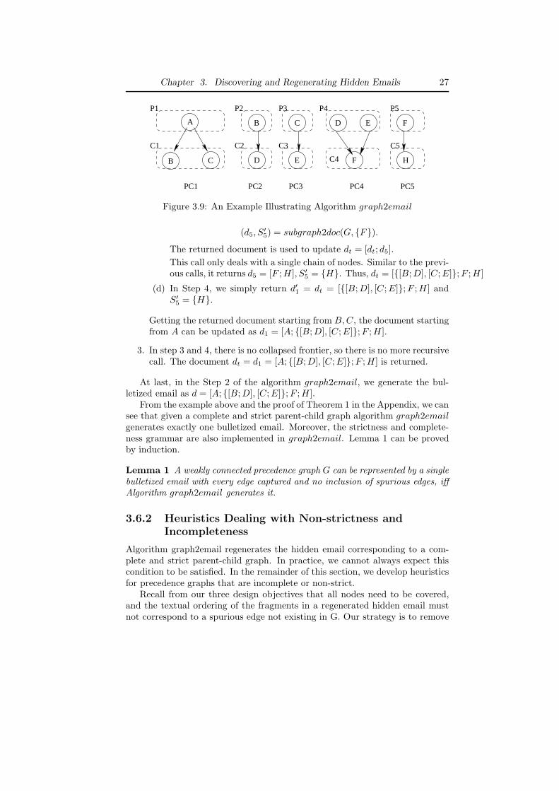
Chapter 3. Discovering and Regenerating Hidden Emails 27
A
C
B
D
C
E
D E F
HB F
PC2 PC3PC1 PC4 PC5
C2
P3
C3
C4
P5
C5
P2
C1
P1 P4
Figure 3.9: An Example Illustrating Algorithm graph2email
(d5, S′5) = subgraph2doc(G, {F}).
The returned document is used to update dt = [dt; d5].
This call only deals with a single chain of nodes. Similar to the previ-ous calls, it returns d5 = [F ; H ], S′
5 = {H}. Thus, dt = [{[B; D], [C; E]}; F ; H ]
(d) In Step 4, we simply return d′1 = dt = [{[B; D], [C; E]}; F ; H ] andS′
5 = {H}.
Getting the returned document starting from B, C, the document startingfrom A can be updated as d1 = [A; {[B; D], [C; E]}; F ; H ].
3. In step 3 and 4, there is no collapsed frontier, so there is no more recursivecall. The document dt = d1 = [A; {[B; D], [C; E]}; F ; H ] is returned.
At last, in the Step 2 of the algorithm graph2email, we generate the bul-letized email as d = [A; {[B; D], [C; E]}; F ; H ].
From the example above and the proof of Theorem 1 in the Appendix, we cansee that given a complete and strict parent-child graph algorithm graph2emailgenerates exactly one bulletized email. Moreover, the strictness and complete-ness grammar are also implemented in graph2email. Lemma 1 can be provedby induction.
Lemma 1 A weakly connected precedence graph G can be represented by a singlebulletized email with every edge captured and no inclusion of spurious edges, iffAlgorithm graph2email generates it.
3.6.2 Heuristics Dealing with Non-strictness and
Incompleteness
Algorithm graph2email regenerates the hidden email corresponding to a com-plete and strict parent-child graph. In practice, we cannot always expect thiscondition to be satisfied. In the remainder of this section, we develop heuristicsfor precedence graphs that are incomplete or non-strict.
Recall from our three design objectives that all nodes need to be covered,and the textual ordering of the fragments in a regenerated hidden email mustnot correspond to a spurious edge not existing in G. Our strategy is to remove

Chapter 3. Discovering and Regenerating Hidden Emails 28
E
B
evictedA B
C D
A B
C ED
==>
E
− A − B # C # D
*
* E
Figure 3.10: Edge Removal for Completeness
some edges from G so that the remaining subgraph G′ still cover all nodes inG and become strict and complete. Recall that we have a completeness andstrictness checker in Step 2(a) and 3(a) of subgraph2doc respectively. Insteadof exiting in both steps, we can call the corresponding heuristics to process Gand continue to generate a bulletized email using Algorithm graph2email andsubgraph2doc. There are many ways to show the removed edges to the user. Onesolution is that we consider the removed edges as a new precedence graph G′′ andapply Algorithm graph2email on G′′. Thus, more than one bulletized emails aregenerated for G and some nodes may appear in both generated emails. Anothersolution is to display the missing edges to the user in the generated email forG′, e.g., a few arrows showing the missing precedence. This is a question of userinterface design, and is not covered in this thesis. We also envision providingthe user with an interface to allow her to reconstruct a possibly totally orderedemail.
Heuristic for Non-strictness
Given the definition of strictness from the previous section, edge removal is aneffective solution for fixing non-strict graphs. There are two kinds of edges thatcan be removed to make the graph strict: (i) the edge that makes two nodes,say x, y, share the same child u; and (ii) the edge between an ancestor and oneof its child nodes that is not itself an ancestor of u. Figure 3.3 shows that theremoval of the edge between b and h makes the graph strict. Removing edge(c, g) also makes the graph strict. Identifying the appropriate edge to removeto overcome non-strictness is easy to incorporate into step 3(a) of Algorithmgraph2email.
Heuristics for Incompleteness
Next we deal with incompleteness. Figure 3.10 shows an incomplete parent-child subgraph because the edge between A and E is missing. Our strategy isto remove the edge between B and E, so that the subgraph involving A, B, C, Dnow becomes a complete bipartite graph. Note that removing an edge can leadto a biclique. In the example above, there is only one biclique left. In general,there may be multiple bicliques.

Chapter 3. Discovering and Regenerating Hidden Emails 29
Algorithm Star-cutInput: a connected bipartite graph G = (L, R, E)Output: a set of edges Ec
1. Find every missing edge ei = (ui, vi), ui ∈ L, vi ∈ R, i ∈ [1, k]. LetU = union(ui), V = union(vi); sort nodes in U in descending order of thenumber of missing edges.
2. For each u ∈ U in descending order, do the following:
(a) Get all missing edges ej = (u, vj)
(b) Add vertex t and edges (vj , t); set the capacity of edge (vj , t) toinfinity.
(c) Get the min-cut cu,t, add cu,t into Ec, and Remove all edges in cu,t
and vertex t
Figure 3.11: A Skeleton of Algorithm Star-cut
We generalize this as a multiple biclique decomposition problem: Given abipartite graph G = (V1 ∪ V2, E) and an edge weight function w, find a subsetof edges Ec ⊆ E with minimum total weight, s.t., G′ = (V1 ∪ V2, E − Ec) canbe partitioned into multiple bicliques, i.e., V1 = V11 ∪ ... ∪ V1k, V2 = V21 ∪ ... ∪V2k, E − Ec = E1 ∪ ... ∪ Ek and Gi = (V1i ∪ V2i, Ei), i ∈ [1, k] is a biclique.
This problem is similar to the maximum edge biclique problem [13], whichis NP-hard. In the following, we present a heuristic algorithm based on themin-cut algorithm.
Let a cut c(u, v) denote a set of edges whose removal disconnects verticesu, v. The capacity of a cut is the total weights of all edges in the cut. c(u, v) iscalled min-cut, iff the capacity of c(u, v) is the minimum among all cuts betweenu, v. For each missing edge (u, v), we can disconnect its two ends by deleting anycut c(u, v). When all the missing edges share the same node u, i.e., ei = (u, vi),we can add an additional node t and edges (vi, t), and set the capacity of edges(vi, t) to a big enough integer(bigger than the degree of vi), the min-cut cu,t
will only contain edges in the original graph, and will therefore give the optimalsolution. The algorithm in Figure 3.11 uses a greedy approach to first processthe node that has the largest number of missing edges incident on it and applythe min-cut in Step 2. To find the min-cut, we use the Edmond-Karp’s maxflowalgorithm [16]. For a flow network with V nodes and E edges, when all edgesare integers and bounded by B, the time complexity is O(|V ||E|).
In order to represent an incomplete parent-child subgraph, the remaininggraph can be multiple bicliques. A single maximum edge biclique, i.e., witha minimum number of deleted edges, is acceptable as well. The maximumedge biclique problem has recently been proved to be NP-complete [53]. Tothe best of our knowledge, Hochbaum’s 2-approximate algorithm [28] is theonly c-approximate algorithm for the edge-deletion problem and is used here as

Chapter 3. Discovering and Regenerating Hidden Emails 30
a comparison. Hochbaum’s algorithm, which is called max-biclique here, alsoapplies the well-known maxflow(min-cut) algorithm. We use Edmond-Karp’salgorithm as well, whose complexity is O(|V ||E|). Both max-biclique and star-cut can be applied in step 2(a) of subroutine subgraph2doc in Figure 3.8. Ourexperiment on a synthetic dataset shows that in most cases, star-cut removesless edges than that of max-biclique. The details can be found in Appendix B.
3.7 Summary
In this chapter, we propose our approach to discover and regenerate hiddenemails. We first discover hidden fragments from each individual email and thenfind hidden fragments that belong to the same hidden email. A precedencegraph is built to represent the relative orders among the hidden fragments.Realizing that the original total textual order among hidden fragments maynot be discovered totally, we develop the bulletized email model to representpartial orderings. A key technical result is that we give a necessary and sufficientcondition for a hidden email to be exactly reconstructed as one bulletized email.Algorithms to regenerate hidden emails are also developed.
31
Chapter 4
Optimizations for Hidden
Email Discovery and
Regeneration
4.1 Introduction
In the previous chapter, we have discussed how to discover and regenerate hiddenemails. Although the previous method has delivered the functionality, it doesnot deliver the efficiency, which is very important as well when dealing with largedataset. In this chapter, we study how to improve the runtime performanceof the hidden email discovery and regeneration. This chapter is organized asfollows.
• In Section 4.2, our overall framework of the discovery and regeneration ofhidden emails is summarized. Based on this framework, we analyze theruntime complexity. We find that the number of emails to compare withand longest common substring comparison are two bottlenecks for runtimeperformance when dealing with large email folders and long emails.
• In Section 4.3 we propose optimization approaches based on email filtra-tion. We first propose a basic email filtration method with word index.Then, we improve it by two filtration methods based on segments and slid-ing windows. We show that the sliding window optimization approach isthe generalized form of all filtration methods we have studied. In Section4.4, we also propose an optimization method for longest common substringcomparison. This approach is also based on the word index and the ideaof segmentation proposed in Section 4.3. For all optimization methods wepropose in both sections, we give conditions that guarantee no decrease inthe accuracy.
• In Section 4.5, we evaluate our framework on the Enron email dataset,which is the largest public accessible email dataset to the best of ourknowledge. First of all, the analysis on the Enron dataset shows thathidden emails are prevalent in the Enron dataset. Second, we study theaccuracy of our framework to regenerate hidden emails on the Enron emaildataset. The experiments show that our framework is accurate even with-out preprocessing of the email corpus. Third, we evaluate the optimization

Chapter 4. Optimizations for Hidden Email Discovery and Regeneration 32
methods proposed in this chapter. Compared with a basic optimizationwith word index only, our methods can greatly reduce the runtime by anorder of magnitude. In addition to the prevalence, accuracy and efficiency,we also evaluated the scalability of our optimization methods by scalingup to larger email folders(up to 12,000 emails). The experiments showthat our methods are scalable to large folders. Moreover, if we adopt aheuristic, we can further improve the runtime performance greatly(about40 times faster) with little decrease(about 2%) in the accuracy.
4.2 HiddenEmailFinder: An Overall
Framework
Figure 4.1 shows the overall algorithm called HiddenEmailFinder, which involvesidentifying all hidden fragments, creating a precedence graph and finally regen-erating bulletized hidden emails. It integrates all the different parts discussedin the previous chapter. Notice that Step 2 of HiddenEmailFinder uses a slightgeneralization of the hidden fragments defined in Section 3.2. It requires thata quoted fragment F be matched against every single email M in the primaryfolder MF , as well as with every email in the reference folders RF1, . . . , RFk.While HiddenEmailFinder finds only hidden fragments and emails in the folderMF , a fragment F is hidden only if it cannot be found in MF , as well as notfound in any of the reference folders RF1, . . . , RFk. The reference folders areuseful because a fragment may be hidden from MF simply because the userfiled the original email into another folder. Thus, to take out the complicationintroduced by email classification, HiddenEmailFinder can take as input multi-ple reference folders for additional checking. The matching in step 2 stops wheneither a match is found (in which case the quoted fragment F is not a hiddenfragment), or a match is not found anywhere (in which case F is consideredhidden).
However, even though HiddenEmailFinder delivers all the required function-alities, a preliminary experimental evaluation revealed that the LCS computa-tion to identify hidden fragments takes most of the runtime. The complexityof identifying the hidden fragments in Step (2) can be analyzed as follows. Letassume that there are totally n emails in the folder MF and reference foldersRF1, ..., RFk. For each email there are c1 new fragments and c2 quoted frag-ments. The length of each fragment is L. The runtime complexity of hiddenfragment identification can be expressed as OHF = O(n ∗ c2 ∗ n ∗ c1 ∗ OLCS) =O(c1c2n
2 ∗ OLCS). Thus, there are two bottlenecks when dealing with largefolders and long emails. The first bottleneck is due to the large number of LCScomputation that may need to be performed between quoted fragments andother emails in the folders, i.e., c1c2n
2. The second bottleneck is due to howwell each single LCS computation is performed, i.e., OLCS . Below we describetwo optimizations to overcome these bottlenecks.

Chapter 4. Optimizations for Hidden Email Discovery and Regeneration 33
Algorithm HiddenEmailFinderInput: email folder MF , and reference email folders RF1, . . . , RFk
Output: a set of bulletized hidden emails in MF
1. For each mail M ∈ MF , extract all the quoted fragments.
2. For each quoted fragment F , match F against all emails in MF as wellas those in RF1, . . . , RFk. In particular, identify the LCS between F andM for every email M ∈ MF or M ∈ RFi for some i. See Section 3.2.Depending on the length of the LCS, F may be declared hidden or not.
3. Find possible overlaps between hidden fragments as described in Section3.3, split them if necessary, and create a precedence graph G.
4. Decompose G into its weakly connected components.
5. For each weakly connected component, do:
(a) Process G with Algorithm graph2email as described in Figure 3.8.If the graph is complete and strict, output the reconstructed hiddenemails. Otherwise, use the heuristics described in Section 3.6.2 todeal with non-strictness and/or incompleteness. Output the recon-structed hidden emails.
Figure 4.1: A Skeleton of Algorithm HiddenEmailFinder
4.3 Email Filtration by Word Indexing
First, we study how to improve the time efficiency by reducing the number ofLCS computation. In other words, we need to reduce the number of emails tobe compared with a quoted fragment without loss of any valid match. Thisoptimization problem can be described as follows.
Given a fragment F and a set of emails MF , find a subset of emails MFsub,such that MFsub includes every email m ∈ MF that contains a fragment F ′
and LCS(F ′, F ) ≥ minLen.The emails in MFsub are called candidates for LCS operation. We need
to compute the LCS between F and every candidate in MFsub until a matchis found. For an email m ∈ MFsub, if LCS(m, F ) ≥ minLen, m is called avalid candidate. Otherwise, it is called an invalid candidate. Our objective is toreduce the number of invalid candidates(cardinality) in MFsub as much as wecan without losing any valid ones.
4.3.1 Word-based Filtration: A Basic Approach
The first optimization is to use a word index, which is known as the invertedindex. Each index entry is of the form: 〈w, Lw〉, where w is a word in the emailcorpus, and Lw is a list of ids of emails containing at least one occurrence of

Chapter 4. Optimizations for Hidden Email Discovery and Regeneration 34
Algorithm EmailFiltration(word-based)Input: the word index, the frequent word list FW , a quoted fragment FOutput: a list of email possibly matching F
1. Tokenize F to a set of words w.
2. For each w not in the list FW , use the word index to identify Lw.
3. Return the unioned list, i.e., ∪w∈F∧w 6∈FW Lw.
Figure 4.2: A Skeleton of Algorithm EmailFiltration(word-based)
w. Given the word index, and a quoted fragment F to be matched, F is firsttokenized to words with all the stop-words removed. Then for each word w, theword index is used to return the list Lw. To support LCS matching between aquoted fragment and an email, a match is allowed even if not all the words arefound in the email. Thus, we take the union of the lists, i.e., ∪w∈F Lw. Thisfiltering process guarantees no false dismissals in the sense that only emails inthe unioned list can ever match F .
Figure 4.2 shows a skeleton of this process. It incorporates an additionaloptimization to reduce the size of the unioned list ∪w∈F Lw. Specifically, itexcludes the most frequent words in the corpus. If we denote this list of wordsas FW , what we actually obtain is the unioned list ∪w∈F∧w 6∈FW Lw. We definethe length of FW as frequent word threshold ft, i.e., the top-ft most frequentwords are kept in FW . In Section 4.5.6, we show that the choice of frequentword threshold has a great impact on the runtime.
4.3.2 Enhanced Filtration with Segments
In the previous word-based filtration approach, we simply union all the emailsthat contain at least one word in the word set W . In this way Msub may in-clude emails that only contain one or two words in F . A valid candidate needsto overlap with F sufficiently and hence has more words in common with F .Moreover, even if an email MF shares many words with F , they may not havea sufficiently long common substring. Such emails shall not be included in thecandidate email set Msub. For example, fragment F contains the following sen-tence:“This morning, Jack came to my house to pick up my book of Database Man-agement Systems.”
Suppose emails M1, ..., M10 share only two common words morning, bookwith F . Thus, in the word-based filtration method, all those 10 emails areselected as candidates and are compared with F . However, with minLen = 40any valid LCS which contains morning also contains Jack and came. Thus,none of M1, ..., M10 can have a LCS of length minLen with F and shall notbe considered as candidates. Consequently, instead of simply using each singleword to filter the invalid candidates, we can use a set of contiguous words, e.g.,

Chapter 4. Optimizations for Hidden Email Discovery and Regeneration 35
Algorithm EmailFiltration(segment-based)Input: fragment F , email folder MF .Output: subset of emails MFsub.
1. Partition F into a sequence of segments(substrings) F = [F1; ...; Fn], suchthat the partition does not split any word in F .
2. For each segment Fi, i ∈ [1, n], do the following:
(a) Tokenize Fi into a set of words Wi.
(b) For each word wj ∈ Wi, get the set of emails Mj ⊆ MF that containswj .
(c) Get the intersection of all Mj as a candidate set of emails for segmentFi, say CMi.
3. Get the union of all emails in CMi as the candidate set of emails MFsub.
Figure 4.3: A Skeleton of Algorithm EmailFiltration(segment-based)
{ “morning”, “Jack”, “came”, “house”}, to filter out more invalid candidates.In other words, we partition the given fragment F into a sequence of segments,and a candidate email has to contain all words of at least one segment. In thisway, we can reduce the number of calls for LCS. This approach is described inFigure 4.3.
The major technical question is that how to partition the fragment F suchthat we can improve the efficiency without loss of accuracy. Obviously, in-creasing the length of a segment can include more words. Since we perform anintersection for the candidates of every word in a segment in Step 2(c), a longersegment implies that more invalid candidates are removed. However, if a seg-ment is too long we may exclude some valid candidates as well. The extreme caseis that the whole F is considered as one segment, which may even exclude validcandidates if the candidate only overlaps with part of F and |F | > minLen. Inthe following we show the existence of an upper bound through one example.Suppose we have a fragment F of length 100, and minLen = 50. If we par-tition F by 25, we get 4 segments, F1, F2, F3, F4, starting from the beginningof F in sequence. For any LCS of length 50, it has to fully cover at least onesegment among F1, ..., F4. Thus, we do not miss any valid candidate email inStep 2(c) of Figure 4.3. If the length of segments is higher than 25, the aboveproperty cannot hold anymore. For example, we can partition F by 26, i.e.,F1 = 26, F2 = 26, F3 = 26, F4 = 22. In this case, if the LCS resides from thesecond character of F to the 51th character of F , it does not fully contain anysegment in F1, F2, F3 and F4. And hence the candidate email is excluded inStep 2(c), because it does not completely include F1 nor F2 due to the absenceof the words in the first and the 51th position. Consequently, we need to findan upper-bound of the length of each segment such that we do not miss anyvalid candidate and reduce as many invalid candidates as we can. Theorem 2describes the upper-bound of segmentation.

Chapter 4. Optimizations for Hidden Email Discovery and Regeneration 36
Theorem 2 Given one string F , which is partitioned into a sequence of seg-ments(substrings) F = [F1; F2; . . . ; Fn], and the threshold of a valid LCS minLen,Let λ = max(|Fi|+|Fi+1|), i ∈ [1, n−1]. For any string F ′, where LCS(F, F ′) ≥minLen, there exists a substring Fi ⊑ F ′ if and only if λ ≤ minLen + 1.
Proof
1. if λ ≤ minLen + 1, i ∈ [1, n], for any string F ′, s.t., LCS(F, F ′) ≥minLen, there exists one segment Fi ⊑ F ′.
Given an arbitrary string F ′, s.t., LCS(F, F ′) ≥ minLen, let l, r denotethe start and end position of LCS(F, F ′) in F respectively. Suppose thecharacters at l and r belong to segments Fi and Fj , i ≤ j respectively.
If j = i, LCS(F, F ′) ⊑ Fi. Hence |Fi| ≥ LCS(F, F ′) ≥ minLen. How-ever, |Fi| < |Fi| + |Fi+1| ≤ minLen + 1, i.e., |Fi| ≤ minLen. Hence,|Fi| = minLen. In other words, l, r are also the left and right boundaryof Fi. LCS(F, F ′) = Fi = minLen
If j = i + 1, LCS(F, F ′) ⊑ Fi + Fj . As LCS(F, F ′) ≥ minLen and|Fi| + |Fj | ≤ minLen + 1, we have the following inequation: minLen ≤LCS(F, F ′) ≤ |Fi| + |Fj | ≤ minLen + 1. Thus, Fi + Fj is at most longerthan LCS(F, F ′) by one character. And hence, either Fi ⊑ LCS(F, F ′) ⊑F ′ or Fj ⊑ LCS(F, F ′) ⊑ F ′.
If j > i + 1, there must exist another segment Fk, i < k < j, Fk ⊑LCS(F, F ′) ⊑ F ′.
Fi Fj
F’
l rLCS(F, F’)
Figure 4.4: Proof of Segmentation Upperbound
2. if λ > minLen + 1, i ∈ [1, n], there exists a string F ′, s.t., LCS(F, F ′) ≥minLen and there does not exist a segment Fi ⊑ F ′.
Suppose |Fi| + |Fi+1| ≥ minLen + 2. Let l denote the beginning and endposition of Fi and r denote the end position of Fi+1.
Let F ′ be the substring from l + 1 to r − 1. Thus, |F ′| ≥ minLen andLCS(F, F ′) ≥ minLen. However, F ′ does not contain either Fi or Fi+1.
�
Corollary 1 If F is partitioned equally, the upper bound of each segment is(minLen + 1)/2.

Chapter 4. Optimizations for Hidden Email Discovery and Regeneration 37
4.3.3 Enhanced Filtration with Sliding Windows
Theorem 2 provides an upper bound on the sum of two consecutive segments,which do not overlap with each other. As we discussed before, we know thatincreasing the length of a segment can reduce the number of candidates but maylose some valid candidates. We want to explore whether we can further increasethe length of each segment, but allowing segments to overlap with each other.Theorem 3 extends Theorem 2 to the general case.
Theorem 3 Given a string F and a sequence of sliding windows Wi, i ∈ [1, n],each of which starts at position si and ends at position ti, si < si+1 and |ti−si| ≤minLen, for any substring Fsub ⊑ F and |Fsub| ≥ minLen, there exists at leastone sliding window which is contained by Fsub, iff ∀i ∈ [1, n − 1], ti+1 − si ≤minLen
In this theorem, we introduce a sliding window W , moving from the left endto the right end of the given fragment F . A candidate email has to containall words in at least one sliding window. The union of candidate emails of allwindows constitute the candidate emails of F . Let GAPi,i+1 = si+1 − si denotethe step of two contiguous sliding windows. Thus, ti+1−si = (ti+1−si+1 +1)+(si+1−si)−1 = Wi+1+GAPi,i+1−1. In other words, the sum of the gap and thelength of its following window need to be less than or equal to minLen+1. Thisapproach is similar to the algorithm in Figure 4.3. But instead of partitioningF into a sequence of segments Fi, we use a sequence of sliding windows Wj tosubstitute segments Fi.
This theorem generalizes the previous theorems. Our previous segmentationmethods can be viewed as special cases of choosing GAP . For example, whenGAP = minLen+1
2 , it corresponds to a sliding window of the length minLen+12
and GAP = minLen+12 , which is Corollary 1. On the other hand, increasing the
window size does not necessarily guarantee less runtime. The total number of
sliding windows for a given fragment can be computed as follows: |F |−minLen
GAP+1.
With the increase of the window size, the total number of sliding windows mayincrease as well. Since we union all the candidates corresponding to each slidingwindow as the candidate for the whole fragment, it is possible that more slidingwindows bring in more candidate emails. Our experiments shows that emailfiltration based on the sliding windows greatly improve the runtime performance.The details can be found in Section 4.5.6.
4.4 LCS-Anchoring by Indexing
While the email filtration algorithm reduces the number of emails to be matchedagainst F , we still need to optimize how well each match can be performed.Recall from Section 3.2 that we extract the longest common substring (LCS)between F and the email currently being checked against. The purpose of usingLCS is to accurately identify all possible hidden fragments. However, the prob-lem with LCS is that its complexity is quadratic in the length of the fragment

Chapter 4. Optimizations for Hidden Email Discovery and Regeneration 38
and the email. For long emails and/or quotations, implementing LCS naively isnot scalable. To address this issue, we propose to extend the word index that weuse to optimize the email filtration step, to optimize LCS. In particular, we aimat reducing the number of comparisons. For each email in the list Lw, we alsorecord the positions at which the word w occurs in the corresponding email, i.e.,each entry in Lw is of the form 〈id, {pos1, . . . , posk}〉. For example, the word“available” may have the following index entry: 〈available, 〈〈id = 17, pos ={89, 3475}〉, 〈id = 278, pos = {190, 345, 3805}〉〉〉.
Then given a quoted fragment F , as before, F is tokenized to words. Foreach word w, and each email M in Lw, we can use the list {pos1, . . . , posk}as “anchors” to facilitate the matching between F and MF . For example,let us say that F contains the word “available.” Then position 89 in email17 is used as an anchor to match up the word “available” in F and email17. By expanding forward and backward from the anchor position as muchas possible, the longest common substring with respect to the anchor positionis formed. Similar anchoring and expansion occurs at position 3475 in email17, and the three specified positions in email 278. If the quoted fragment istokenized to multiple words, the above process is conducted for each word w,and the longest common substring is selected. Figure 4.5 gives a skeleton ofthis optimization step called LCS-anchoring. This optimization is intended tobe used in step 2 and 3 of HiddenEmailFinder. Furthermore, according to ouranalysis in Theorem 2, we can also use segmentation in the LCS computation.Given two fragments F1, F2, we can partition one fragment, e.g., F1, into asequence of segments, each of which is no longer than (minLen + 1)/2. Asdescribed in Theorem 2, a valid overlap of length minLen must contain at leastone segment. Hence, we only need to anchor one word in each segment for LCScomparison.
4.5 Empirical Evaluation
4.5.1 The Enron Email Dataset
The Enron email dataset was made public by the US Federal Energy Regu-latory Commission during the ex-Enron investigation. This dataset containsabout half a million messages belonging to 151 users and 3500 folders with allattachments deleted. For most of the results reported below, we focus on themost common inbox folders of the users. Among the 151 users, 137 have aninbox folder. The number of emails in those folders ranges from 3 to 1466. Theaverage and median number of emails are 327 and 223 respectively. The En-ron corpus has been used for social network analysis, email classification, etc.Many analyses and preprocessing have been done on the Enron dataset[51]. Forexample, the SIAM’05 Workshop on Link Analysis, Spam Detection and Anti-terrorism published several indexes of the Enron dataset. In our experiments,we use their word indexes instead of building our own. The word index con-tains 160,203 unique words. Recall that whenever we refer to a frequent word
Chapter 4. Optimizations for Hidden Email Discovery and Regeneration 39
Algorithm LCS-AnchoringInput: the word index, the frequent word list FW , a quoted fragment F , andan email MOutput: the LCS between F and M
1. Tokenize F to a set of words w, removing the stop-words and keeping onlythose not in FW .
2. If M does not appear in any of the lists Lw for all the remaining w’s,return the empty string.
3. Otherwise, for each such w,
(a) for each anchor position posi
i. Align w at posi in M and F .
ii. Expand the matched substring forward and backward as muchas possible.
4. Return the longest matched substring in the nested loop.
Figure 4.5: A Skeleton of Algorithm LCS-Anchoring
threshold (ft), we mean that the top-ft words are considered too frequent tobe used in EmailFiltration or LCS-Anchoring. Below we vary ft from 1000 to80,000, corresponding to about 0.6% and 50% of the words respectively.
In our experiments we have thoroughly tested all critical aspects of ourframework for hidden email discovery and regeneration. First, we examine theprevalence of hidden fragments in the inbox folders. We also examine the per-centage of hidden fragments that can be recollected from other folders of thesame user. Then, we evaluate the accuracy of our framework. The impact ofsignatures and minLen on the accuracy is discussed. We also evaluate the ef-fectiveness of the optimization algorithms EmailFiltration and LCS-Anchoring.We compare the savings in runtime against the possible reduction in the qualityof the output (i.e., reconstructed emails). Realizing the possibility of large emailfolders for applications such as email forensics, we study the scalability of ourframework. All runtime figures were obtained based on experiments done on aSun Fire 880, 900MHz UltraSPARC-III machine.
4.5.2 Prevalence of Emails Containing Hidden Fragments
For each user in the Enron dataset, we identify all the hidden fragments in theinbox folder. Figure 4.6(a) shows the number of emails that contains at leastone hidden fragment. Due to lack of space, we only show the largest 50 inboxfolders sorted by ascending folder size (ranging from 338 to 1466 emails). Ascan be seen from the figure, there are 5 inbox folders with more than 300 emailscontaining at least one hidden fragment.

Chapter 4. Optimizations for Hidden Email Discovery and Regeneration 40
While Figure 4.6(a) shows the absolute values, Figure 4.6(b) displays thepercentage of emails containing at least one hidden fragment (i.e., relative tothe folder size). Because percentage may not make sense for small folders, weexclude folders with less than 50 emails. The x-axis of the graph shows thepercentage, ranging from 0% to 60%. The y-axis shows the number of userswith the given percentage. It is interesting to see that about half of the usersare within the range of 15% to 30%, i.e., 15% to 30% emails contain hiddenfragments.
0
100
200
300
400
500
600
user folder(sorted by the folder size)
# of
em
ails
con
tain
ing
hidd
en fr
agm
ents
# of emails containing hidden fragments
(a) Emails with Hidden Fragments
0 10 20 30 40 50 600
5
10
15
20
25
percentage of emails containing hidden fragments (%)
num
ber o
f use
rs
(b) Histogram on the Percentage of Emails Containing Hidden Frag-ments
Figure 4.6: Emails Containing Hidden Fragments

Chapter 4. Optimizations for Hidden Email Discovery and Regeneration 41
Note that so far the analysis is based on emails in the inbox only. That isto say, a quoted fragment is designated to be hidden, as long as it cannot befound in the inbox folder. The reader may wonder whether hidden fragmentsjust represent a phenomenon of the user being diligent in filing her emails intoan appropriate folder. To examine this effect, we check other folders of the sameuser. Hereafter, we refer to a hidden fragment as “global” if it is a fragment thatcannot be found in all the folders of the user. We refer to a hidden fragmentas “local” if it is a hidden fragment within the (inbox) folder, but is otherwisefound in some other folder of the user. Let us denote the numbers of globaland local hidden fragments by ng and nl respectively. We define the recollectionrate as the ratio of nl/(nl + ng). That is to say, the closer the ratio is to 1, thesmaller is the number of global hidden fragments.
Figure 4.7 shows a histogram of the recollection rates for all the users. Itis interesting to see that most users have a recollection rate of less than 15%.That is to say, there is less than 15% of hidden fragments that can be found inthe other folders of the user. For the Enron dataset, the average and median(nl +ng) values are 211 and 102 fragments respectively. Using the median figureof 102 hidden fragments as an estimation, a recollection rate of less than 15%corresponds to at most 15 local hidden fragments and at least 87 global hiddenfragments. Thus, hidden fragments do not seem to be simply a phenomenon ofthe user filing the emails to other folders; they are truly missing from the user’sfolders.
0 5 10 15 20 25 30 350
5
10
15
20
25
30
recollection rate(%)
num
ber o
f use
rs
Figure 4.7: Histogram of Recollection Rates
While it is clear that hidden fragments are prevalent in the Enron corpus,the immediate question here is how general this phenomenon is for a “typical”real user. Let us review how the Enron dataset was prepared. As reportedin [9], emails were deliberately deleted from the first published version of theEnron dataset on the users’ request for privacy and redaction purposes. It isestimated that about 8% of the emails were deleted to form the current version.Consider the following two aspects:

Chapter 4. Optimizations for Hidden Email Discovery and Regeneration 42
• First, the deleted emails are believed to be more personal in nature. Itis reasonable to assume that they were less likely to be quoted in manyEnron business emails.
• Second, the average number of reconstructed hidden emails per user isabout 60. Given that the average inbox folder size is 327 emails, if the 8%of the deleted emails were evenly distributed in the inbox folder of eachuser, this would correspond to 26 emails in the folder. The gap between26 and 60 is significant.
The question of whether hidden fragments are prevalent in a typical user’sfolder is hard to be answered definitively. But for the two reasons discussedabove, the abundance of (global) hidden fragments we found in the Enron corpusmay well generalize to other real datasets.
There is actually another interesting point to make here. Emails were deletedpartly to protect privacy. However, some of these deleted emails may be recov-erable from emails in other folders. Thus, if there is an initial set of emails tobe protected, the framework that we develop here can help to strengthen theprotection by identifying other emails quoting the initial set.
4.5.3 Accuracy Evaluation
Dataset setup
So far, we have discussed the abundance of hidden emails. A natural question isthat whether our framework generates hidden emails correctly. Hidden emailsare hidden because we do not know the original emails. Thus, it is difficultto directly evaluate the quality of the regenerated hidden emails. In this ex-periment, we create some hidden emails artificially to perform an evaluation.We first delete some emails from the folder and create some “known” hiddenemails. Then we apply HiddenEmailFinder to regenerate hidden emails from theremaining emails. Finally, we compare the regenerated emails with the deletedones and see to what extent the deleted emails are recovered. Specifically, weuse all email conversations in the 10 largest inbox folders in the Enron datasetas the test folders. The total number of email conversations we find is 296. Theroot emails in those conversations are deleted to create some hidden emails.Since the root emails are quoted by the other emails in the conversation, weapply HiddenEmailFinder to those emails to regenerate the deleted roots.
In our preliminary experiments, we find that there are two major factors thatinfluence the accuracy. First, the accuracy of the regeneration depends on thesuccessful identification of quotations. Since quotations are free text and differ-ent email clients treats quotations in different ways, quotation identification isitself a research problem. Second, HiddenEmailFinder use string overlapping toidentify hidden fragments belonging to the same hidden email. However, twodifferent hidden emails may contain a long common substring. One obviouscase is signature, which is a text fragment automatically attached to an email.In addition, this is also likely to happen when two hidden emails are about the

Chapter 4. Optimizations for Hidden Email Discovery and Regeneration 43
same topic. In such cases, two hidden emails may be regenerated as one hiddenemail by HiddenEmailFinder. We call these two cases as “signature overlap”and “content overlap” respectively. Signature overlap is considered as noise forour framework and need to be identified in the preprocessing stage.
We preprocess the test folders as follows. First of all, we delete all existinghidden emails from the test folders, so that it contains no hidden email beforethe removal of the roots. We call this dataset as “basic” and use it as a basicdataset in our experiment. Then, we make sure that all emails are quoted withstandard quotation marks and can be discovered successfully. Finally, we deletesignatures from the original email. This dataset is called a “cleansed” dataset.Thus, in both datasets all quotations can be identified correctly and all theregenerated hidden emails are related to the deletion of root emails.
Evaluation criteria and the result
We study how the deleted root emails are regenerated into hidden emails. Oneroot email may be recovered as one hidden email, multiple hidden emails ornot discovered at all. In our experiments, all deleted roots are discovered bythe HiddenEmailFinder. There are 4 types of mapping between deleted rootsand the regenerated hidden emails: 1 → 1, m → 1, 1 → m and m → k,(m > 1, k > 1). Figure 4.8 shows an example of the 4 types of mappingdescribed above. Ri, i ∈ [1, 6] are 6 deleted roots, and Hj , j ∈ [1, 7] are 7regenerated hidden emails.
R1 R2 R3 R4 R5 R6
H1 H2 H3 H4 H5 H6 H7
Figure 4.8: Example of Mapping Between Roots and Regenerated HiddenEmails
• 1 → 1, a deleted root is regenerated exactly as one hidden email, whichdoes not contain information from other deleted roots, e.g., R1 and H1.
• 1 → m, one deleted root is regenerated into m hidden emails, which onlycontain fragments from this root, e.g., R2, H2 and H3.
• m → 1, m deleted roots are regenerated as one hidden email, which onlycontains fragments from those m roots,e.g., R3, R4 and H4.
• m → k, m deleted roots are regenerated into k hidden emails. That isto say one regenerated hidden email contains multiple roots, and one rootis reconstructed into multiple hidden emails, e.g., R5, R6, H5, H6 and H7.This cases is a hybrid case of the previous ones. For example, roots R5
and R6 have a long enough common substring. During the regeneration

Chapter 4. Optimizations for Hidden Email Discovery and Regeneration 44
process, R5 is discovered as H5, H6, and R6 is regenerated as H6, H7,where H6 is the common substring shared by two roots. Thus, R5 and R6
are regenerated as 3 hidden emails H5, H6 and H7.
1 → 1 m → 1 1 → m m → kbasic dataset 87.2% 5.2% 0.2% 7.4%cleansed dataset 96.5% 2.0% 1.5% 0%
Table 4.1: Percentage of Root Mapping Types
We apply HiddenEmailFinder to the emails in the test folders and examinethe root mapping types described above. In this experiment, we set minLen =100, f t = 1000. Table 4.1 shows the percentage of the 4 types respectivelyin both the basic and cleansed dataset. In the basic dataset, the percentageof 1 → 1 type is 87%. This shows that our method can reconstruct hiddenemails effectively even in the basic dataset with signatures and non-standardquotations. Among the inaccurate cases, 21 roots(5.2%) belong to the m → 1category. As described before, the major reasons are signature overlapping andcontent overlapping among those roots. Out of the 21 roots, 17 roots are dueto signature overlapping and only 4 roots belong to the content overlappingcategory.
In the cleansed dataset, most of the deleted roots, about 96%, are discoveredas single hidden email. Since the cleansed dataset does not contain signature,only 4 roots (2%) are regenerated as one hidden email due to content overlap-ping. In addition, there are about 1.5% roots in the 1 → m category. The onlyexplanation we found for this is the modification of the quotations, which causessome hidden fragments originating from the same hidden email not to overlapsufficiently, and hence to be identified as different hidden emails.
Accuracy w.r.t. minLen
In the identification of hidden fragments and in the construction of the prece-dence graph (steps 1 and 2 of HiddenEmailFinder), a key parameter is thechoice of minLen, the minimum length for the algorithm to declare a match.This choice affects whether one quoted fragment is considered a hidden fragmentor not (Section 3.2), and whether a fragment need to be split (Section 3.3). Forinstance, a larger minLen can avoid incorrect matching of common sentences
40 100 200 3001 → 1 84.2% 87.2% 90.0% 88.7%m → 1 9.0% 5.2% 2.1% 2.0%1 → m 0.2% 0.2% 1.3% 3.4%m → k 6.6% 7.4% 6.7% 5.9%
Table 4.2: Percentage of Different Types w.r.t. minLen on Uncleansed Dataset

Chapter 4. Optimizations for Hidden Email Discovery and Regeneration 45
11
4
0 0
23
17
1010
0
5
10
15
20
25
40 100 200 300
num
ber
of
roots
content overlapping
signature overlapping
Figure 4.9: Type of Overlapping w.r.t. minLen
and quotation, and hence we have less m → 1 cases. On the other hand, it mayalso miss short quotations, and create more hidden fragments.
Table 4.2 shows the change of accuracy with different minLen from 40 to300 on the basic dataset. From this table we see that with the increase ofminLen from 40 to 200, the percentage of 1 → 1 increases for about 6% witha corresponding decrease of m → 1 case from 9% to 2.1%. The reason liesin that higher minLen can reduce invalid overlappings. Figure 4.9 shows thisin detail. The x-axis is the minLen, and the y-axis is the number of rootsinvolved in either type of overlapping. This figure clearly indicates that forboth types, the number of roots decreases with the increase of minLen. WhenminLen = 200 no root is regenerated as m → 1 case due to content overlapping.At the same time, the signature overlapping drops to 10, which is 43% of thatof minLen = 40. This validates our previous analysis that a large minLen mayreduce invalid overlappings.
On the other hand, the number of roots in 1 → m category increases with theincrease of minLen. This reveals that more roots are regenerated as separatehidden emails. This also explains the slight drop of 1 → 1 cases when minLenincreases from 200 to 300.
4.5.4 Word-based Email Filtration and LCS-Anchoring
In this section, we study the effectiveness of the optimization heuristics of Email-Filtration and LCS-Anchoring. We measure the runtime of step 2 of Hidden-EmailFilter, which is the dominant step. We also record the number of recon-structed hidden emails as a way to measure the output quality of HiddenEmail-

Chapter 4. Optimizations for Hidden Email Discovery and Regeneration 46
Finder. The intent is to observe the tradeoff between runtime efficiency andoutput quality. In the following sections, we use the 137 inbox folders as thetest dataset.
We design our experiments in the following way. In the first round of exper-iments, we only apply the heuristic of word-based EmailFiltration and changethe frequent word threshold (ft). We vary ft from 500 to 80,000. In thesecond round of experiments, we apply both word-based email filtration andLCS-Anchoring. For both rounds, we record the runtime and the number ofreconstructed hidden emails for all the inbox folders.
Figure 4.10(a) shows the median runtime performance. The x-axis is drawnin log scale of the frequent word threshold ft. Let us first focus on the curveapplying only the EmailFiltration algorithm. The basic, unoptimized version ofHiddenEmailFinder corresponds to the case when ft = 0. The median runtimefor this case is about 10 minutes, which is not shown in the figure. As the valueof ft increases, the runtime improves by as much as 2 orders of magnitude,down to less than 10 seconds for ft = 10, 000.
The second curve in Figure 4.10(a) shows the additional gain in efficiencywhen LCS-Anchoring is applied on top of EmailFiltration. The gap between thetwo curves shows that there is a definite bonus in applying LCS-Anchoring. Thegain becomes smaller as ft increases because EmailFiltration alone has alreadyeliminated a lot of emails required for matching, thereby reducing the numberof times that LCS-Anchoring is performed.
Now the question is whether the significant gain in efficiency is achievedthrough reduced quality. Figure 4.10(b) shows that the number of reconstructedhidden emails when ft changes from 1000 to 80,000. The case when ft = 0 is notshown in the figure, but is identical to the value for ft = 1000. As ft increasesfrom 1000 to 80,000, the number of reconstructed hidden emails increases veryslightly, reflecting the reduced connectivity of the precedence graph. Given thatthe two curves in Figure 4.10(b) almost completely coincide, it is clear thatboth EmailFiltration and LCS-Anchoring can bring about a gain in efficiencywithout causing a degradation in the output quality.
Figure 4.10(a) does not include the average runtime because there is a largediscrepancy between folders on how long it takes to process them. Figure 4.10(c)shows the extreme case of the top-10 largest folders. Among these top-10 folders,the median folder contains 1,152 emails, with 37 emails each longer than 1,000words. Large folders and long emails take significantly more time than thesmaller ones. The two curves in the figure show the median runtime acrossthe 10 folders when EmailFiltration alone and when EmailFiltration and LCS-Anchoring. Like in Figure 4.10(a), it is clear that both techniques are effective.For example, when ft = 10, 000, corresponding to 6% of the total number ofunique words, the median runtime even for the top-10 largest folders is nowdown to 28 seconds. But unlike in Figure 4.10(a), this time the gap is farmore significant whether LCS-Anchoring is applied. This convincingly showsthe importance of LCS-Anchoring for long emails and large folders.

Chapter 4. Optimizations for Hidden Email Discovery and Regeneration 47
0
20
40
60
80
100
120
140
1000 10000 100000
frequent word threshold (in log scale)
run
tim
e(s
ec)
median: EmailFiltering
median: EmailFiltering + LCS-Anchoring
(a) runtime
0
5
10
15
20
25
30
35
40
45
50
1000 10000 100000
frequent word threshold (in log scale)
# o
f re
colle
cte
d h
idden e
mails
median: EmailFiltering + LCS-Anchoring
median: EmailFiltering
(b) number of reconstructed hidden emails
0
200
400
600
800
1000
1200
1400
1600
1800
1000 10000 100000
frequent word threshold (in logscale)
run
tim
e (
se
c)
median: EmailFiltering
median: EmailFiltering + LCS-Anchoring
(c) runtime of top-10 largest folders
Figure 4.10: Effectiveness of Optimizations

Chapter 4. Optimizations for Hidden Email Discovery and Regeneration 48
4.5.5 Email Filtration by Sliding Windows
We evaluate empirically the runtime performance with respect to different win-dow(or GAP) size. In these experiments, we first set the window size asminLen+1
2 , which is the maximum segment size described by Corollary 1. Then,we increase the window size based on Theorem 3. In this experiment, we setminLen = 200, f t = 1, 000. Figure 4.11(a) shows the runtime performancewhen changing window size. The x-axis is the window size, and the y-axis is theaverage runtime of all inbox folders. Figure 4.11(a) shows that when the windowsize is 100, which is the maximum non-overlapping window(segment) size, theaverage and median runtime are 9 and 2 seconds respectively. In comparison,when using word-based email filtration approach it takes 126 and 24 secondsrespectively. In other words, by using the sliding windows(or segmentations),the runtime is improved by about 12 times. When we change the window sizefrom 100 to 190, the maximum and minimum average runtime is 14 and 8, bothof which are much less than that of the word-based filtration method. More-over, the runtime decreases from 9 seconds to 8 seconds when the window sizeincreases from 100 to 105. This validates our previous analysis in Section 5that longer windows include more words and hence remove more invalid candi-dates. However, with the increase of the window size afterwards, the runtimekeeps increasing. When the window size is 190, the average runtime reaches14 seconds. Recall our previous analysis that the increase of the window sizecan bring in more sliding windows, and hence may result in more candidates.The decrease and increase in Figure 4.11(a) validates the previous analysis. Inaddition, Figure 4.11(b) shows the number of times LCS is computed w.r.t. thewindow size. We can see that this curve shows a similar trend in accordancewith that of the average runtime in Figure 4.11(a). This supports the analysisof the bottlenecks in runtime performance.
Other than the runtime performance, Figure 4.11(c) shows the number ofhidden fragments found when changing window size. This figure shows thatthe number of discovered hidden fragments hardly varies when the window sizechanges, which is expected according to Theorem 3.
4.5.6 Scalability
In the Enron dataset, the size of the 137 inbox folders ranges from 3 to 1466.However, for email applications, e.g., email forensics, it is possible that theinvestigators need to handle much larger email folders. In the following, westudy the scalability of HiddenEmailFinder to large folders. As discussed inSection 5, the identification process accounts for most of the time consumptionand is the focus of our experiments. We apply both EmailFiltration and LCS-Anchoring heuristics in the following experiments.
We design the scalability experiments as follows. We select the 10 largestinbox folders from the Enron dataset as the test dataset. The number of emailsin each folder ranges from 1008 to 1466. For the ease of presentation, we sortthem by the folder name and call them as A1, . . . , A10 in order. Then we cre-

Chapter 4. Optimizations for Hidden Email Discovery and Regeneration 49
0.00
2.00
4.00
6.00
8.00
10.00
12.00
14.00
16.00
90 110 130 150 170 190 210window size
runtim
e (
seconds)
average
median
(a) Runtime to discover hidden fragments
0
10
20
30
40
50
60
70
90 110 130 150 170 190 210window size
num
ber
LC
S c
om
puta
tion
average
median
(b) # of calls for LCS
0
50
100
150
200
250
90 110 130 150 170 190 210window size
num
ber
of
hid
den f
ragm
ents
average
median
(c) # of hidden fragment discovered
Figure 4.11: Email Filtration Based on Sliding Windows

Chapter 4. Optimizations for Hidden Email Discovery and Regeneration 50
ate a sequence of virtual folders from A1, . . . , A10 and use them to test thescalability. Each virtual folder is the union of some distinct folders from thetest dataset. There are many ways to generate the virtual folder. For thepurpose of scalability, we choose to generate them incrementally as follows.A virtual folder V Fi, i ∈ [1, 10] consists of i individual folders {A1, . . . , Ai}.Hence, V F1, . . . , V F10 are a sequence of folders that contain increasing numberof emails, and V Fi ⊂ V Fj for all 1 ≤ i < j ≤ 10. The smallest virtual folderV F1 contains 1143 emails, and the largest virtual folder V F10 contains 12,259emails.
0
100
200
300
400
500
600
700
800
900
0 2000 4000 6000 8000 10000 12000 14000
number of emails in the folder
run
tim
e to
dis
co
ve
r h
idd
en
fra
gm
en
ts
VF: 10 folders with dasovich-j/inbox
VF': 9 folder without dasovich-j/inbox
Figure 4.12: Runtime to Identify Hidden Fragments
We apply the HiddenEmailFinder to those 10 virtual folders and examineits performance. Figure 4.12 shows the runtime with respect to different virtualfolders. The x-axis is the number of emails in a folder, and the y-axis is theruntime to identify the hidden fragments. In this experiment, we set ft =20, 000, which is about 12% of the total number of words in the Enron dataset.The V F series in Figure 4.12 shows the runtime for V F1, . . . , V F10. The minimalruntime is 2 seconds at the size 1143, and the maximal runtime is about 800seconds at the size of 12,259. Figure 4.13 shows the runtime to identify hiddenfragments for each individual folder A1, . . . , A10 respectively.
We notice that, in general, the runtime keeps increasing with the increaseof the folder size, and the increase is higher than additive. For example, theruntime of V F2 = {V F1, A2} is 13 seconds, which is larger than the sum of the
folder name A1 A2 A3 A4 A5 A6 A7 A8 A9 A10
runtime 6 4 104 11 3 15 2 15 12 25
Figure 4.13: Runtime to Identify Hidden Fragments of 10 Individual Folders

Chapter 4. Optimizations for Hidden Email Discovery and Regeneration 51
runtime of V F1 (6 seconds) and that of A2 (4 seconds). In Section 5, we showthat the runtime complexity is O(c1c2n
2OLCS). Our optimization algorithmscan greatly improve the runtime performance, but empirically the runtime isstill higher than linear.
Another interesting phenomenon is that the first two virtual folders haveruntime of 6 and 13 seconds respectively, while the third one increases dramati-cally into 132 seconds. From the third to the tenth folder, the runtime increasesalmost linearly with respect to the number of emails in the folder. Since we cre-ate virtual folders in an incremental mode, i.e., V F3, . . . , V F10 all contain A3,we suspect that the folder of A3 = dasovich− j/inbox is the one that accountsfor the dramatic increase in runtime.
Figure 4.13 shows that it takes 104 seconds to discover hidden fragmentsin A3, while the average time of other folders are around 10 seconds. Thereason lies in the length of emails. The average number of words per email inA3 is about 800. In contrast, this average is about 300 for the other folders.According to the previous analysis, long emails, which contains more distinctwords, are supposed to have more chances to be compared with other quotedfragments. On the other hand, long quotations need to compare with moreemails to identify whether they are hidden or not. At the same time, it takesmore time for each individual LCS computation. These reasons explain whyA3 dramatically increases the runtime when it is included. Consequently, thisresult shows that long emails are critical to the runtime performance.
Thus, we remove A3 from the test dataset and create another sequence of vir-tual folders, V F ′
1, V F ′2, . . . , V F ′
9 as described before, e.g., V F ′3 = {A1, A2, A4}.
The size of V F ′i is different from that of V Fi, but very close. The runtime is
shown in the V F ′ series in Figure 4.12. We can see that the runtime of V F ′i , i ∈
[3, 7] is about half of the corresponding runtime of the folders V Fi, i ∈ [3, 7].The runtime for V F ′
9 is 400 seconds which is about two thirds of the time spentfor V F9. By comparison of the two series, it is obvious that A3 is critical to theoverall runtime.
The above experiments show the scalability of our framework to large folderswhere we set ft = 20, 000. We find that large folders and long emails play animportant role in the runtime performance. One may still argue that the runtimeis not fast enough for large email forensics applications, where the number ofemails are much larger than 10,000. As discussed in Section 4.3, the use of ftprovides us flexible choice to improve the runtime performance. The larger isthe ft, the faster is it to discover hidden fragments. Figure 4.14(a) shows theruntime when changing ft from 5,000 to 80,000 for virtual folder V F3, V F6 andV F10. The x-axis is the frequent word threshold ft and the y-axis is the runtimeto discover hidden fragments. Let us take folder V F10 which contains 12,599emails as an example. We see that with the increase of ft from 5,000 to 80,000,the runtime of V F10 decreases dramatically from 8332 seconds to 203 seconds.The most significant improvement takes places between 5,000 and 20,000. Whenft = 20, 000 the runtime decreases to about 800 seconds. All three curves showsthe similar shape as that of V F10. The relative ratio in runtime among differentfolders does not change much, e.g., V F10/V F6 is about 2.1. At the same time,
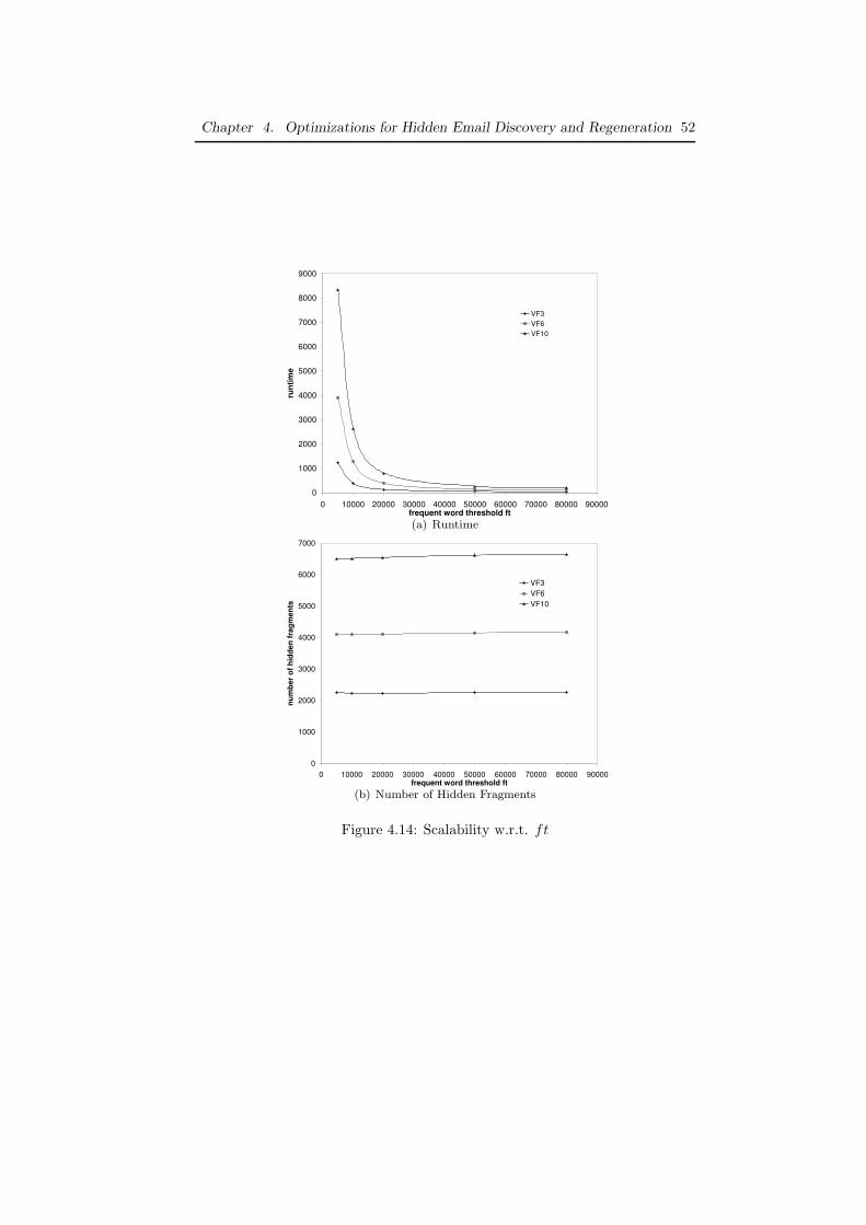
Chapter 4. Optimizations for Hidden Email Discovery and Regeneration 52
0
1000
2000
3000
4000
5000
6000
7000
8000
9000
0 10000 20000 30000 40000 50000 60000 70000 80000 90000frequent word threshold ft
run
tim
e
VF3
VF6
VF10
(a) Runtime
0
1000
2000
3000
4000
5000
6000
7000
0 10000 20000 30000 40000 50000 60000 70000 80000 90000frequent word threshold ft
nu
mb
er
of
hid
den
fra
gm
en
ts
VF3
VF6
VF10
(b) Number of Hidden Fragments
Figure 4.14: Scalability w.r.t. ft

Chapter 4. Optimizations for Hidden Email Discovery and Regeneration 53
the discovered hidden fragments increases from 6507 to 6655 as shown in Figure4.14(b). The increase is about 2.3% of that of ft = 5000. The above experimentsshow that by using ft, we can greatly improve the runtime performance withsome tolerable decrease in accuracy. The use of ft is flexible, and it is up to theuser to decide the tradeoff she can accept.
4.6 Summary
This chapter studies the optimization problem of the basic HiddenEmailFinderalgorithm to deal with large folders and long emails. The two optimizationsare based on word indexing to reduce the number of emails that need to bematched and to reduce the amount of effort required to find the LCS between thefragment and the email under consideration. In addition, we give conditions thatguarantee no decrease of the accuracy. This framework can also be applied tothe email forensic and email mining applications, where discovering informationfrom emails is crucial for the investigators. It can also be used for extractingemail conversations from an email folder as will be discussed in Chapter 5. Asa side effect, given an initial set of emails to be protected, HiddenEmailFindermay be used to strengthen the protection by identifying other emails quotingthe initial set.
Another important result of this chapter is the Enron case study. Fromour experimentation, many valuable lessons are learned. First, we observe thatglobal hidden fragments are prevalent in the Enron corpus, and that HiddenE-mailFinder serves to reconstruct the hidden emails. There are good reasons tobelieve that the prevalence may well generalize to other real datasets, therebyjustifying the importance of the hidden email reconstruction problem. Second,we study the accuracy of our framework and show that the accuracy is high evenon a basic version of the Enron dataset. We also show that both the EmailFil-tration and the LCS-Anchoring techniques are effective in providing scalabilityto large folders and long emails. They can greatly improve the runtime perfor-mance, while not compromising the output quality. Last but not least, we studythe scalability of our framework and shows that with the optimization methodsand the proper use of frequent word threshold, our framework is scalable tolarge folders with little loss of accuracy.

54
Chapter 5
Summarizing Email
Conversations with Clue
Words
5.1 Introduction
In the previous chapters, we have discussed how to discover and regenerate hid-den emails from the quotations of an email conversation. With all the messagesbeing identified, either explicit or hidden ones, in this chapter we study how toextract and represent the structure of an email conversation. Based on this con-versation structure, we further study how to summarize an email conversation.
In Section 5.2, we propose using the fragment quotation graph to captureconversations. Based on an analysis of the quotations embedded in emails, thegraph provides a fine representation of the referential structure of a conversa-tion. An important characteristic of this graph is that the hidden emails of thisconversation are also included into this graph.
In Section 5.3, we propose an email summarization method, called Clue-WordSummarizer (CWS), based on a novel concept called clue words. A clueword from a node is a word (modulo stemming) that appears also in its parentnode(s) and/or child node(s) in the quotation graph. It is important to notethat a clue word takes into account simultaneously (part of) the content andthe structure of the quotation graph. Moreover, CWS is unsupervised and canproduce summaries of any size as requested by the user.
It is an open question how human would summarize email conversations.Thus, in Section 5.4, we present results of a user study on summarizing 20conversations from the Enron data set. Not only does this study provide a goldstandard to evaluate CWS and other summarization methods, but also confirmthe importance of clue words and hidden emails to human summarizers.
In Section 5.5, we evaluate the effectiveness of CWS on the Enron data set.We propose two evaluation metrics Sentence Pyramid Precision and ROUGE.Based on the two evaluation metrics, we compare CWS with other summariza-tion approaches. Our preliminary results show that both the quotation graphand clue words are valuable for summarizing email conversations.

Chapter 5. Summarizing Email Conversations with Clue Words 55
5.2 Building the Fragment Quotation Graph
As we have discussed in Chapter 1, email conversations can be more complicatedthan a simple email thread. One reply can comment on different part of the pre-vious emails separately by selective quotations. The existence of the quotations,especially selective quotations, provides a structural clue on how the replyingemail is organized. In this section, we build a fragment quotation graph, whichis based on the quotation analysis, to capture the email conversation structure.
For any given email folder, there may be multiple email conversations. Tocapture these different conversations, we assume that if one email quotes anotheremail, they belong to the same conversation. We use a fragment quotationgraph to represent the conversation. A fragment quotation graph G = (V, E)is a directed graph, where each node u ∈ V is a text unit in the email folder,and an edge (u, v) means node u is in reply to node v. We are aware that thisframework cannot represent every kind of email conversations. For example,there are cases where the original email is not quoted by the replies, and thereare cases where the quotation is irrelevant to the topic discussed. Nonetheless,we believe that fragment quotation graphs can be applied to many practicalsituations.
5.2.1 Identifying Quoted and New Fragments
The first step to build the quotation graph is to identify quoted and new frag-ments within each email. Quotation identification is itself a research prob-lem [72]. Here we assume that there exist one or more quotation markers (e.g.,“>”) that are used as a prefix of every quoted line. We define the quotationdepth of a line as the number of quotation markers “>” in the prefix. Thequotation depth reflects the number of times that this line has been quotedsince the original message containing this line was sent. A quoted fragment is amaximally contiguous block of quoted lines having the same quotation depth.A new fragment is a maximally contiguous block of lines that are not prefixedby the quotation markers. In other words, an email can be viewed as a sequenceof quoted and new fragments.
For convenience, we use Mi.quote and Mi.new to denote the set of quotedand new fragments in email Mi respectively. We use Mi.frag to denote thesequence of fragments, both quoted and new ones. The order of the fragmentsis in accordance to their textual order in Mi. We denote the quotation depthof fragment F as F.qtDepth. The quotation depth of a new fragment is definedas 0.
5.2.2 Creating Nodes
Given an email folder MF = {M1, . . . , Mn}, we construct a fragment quotationgraph G as follows. After the aforementioned identification of quoted and newfragments in each email Mi in MF , the first step is to identify distinct fragments,each of which will be represented as a node in the graph.

Chapter 5. Summarizing Email Conversations with Clue Words 56
b> a
E2c> b> > a
E3 E4de> c> > b> > > a
E5gh> > d> f> > e
E6> gi
> hj
aE1
(a) Conversation involving 6 Emails
ba c
e
d
f
h
g i
j
(b) Fragment Quotation Graph
Figure 5.1: A Real Example
Note that when a user quotes an email, the user might perform variousactions, as she can edit the fragments as free text. She can quote the exactsequence verbatim; or she can delete some parts of it. For example, a newfragment from an earlier email can be of the form NF1 = 〈F1, F2, F3〉. In alatter email, a quoted fragment may be QF2 = 〈F1, F3〉. In another email,it may appear as QF3 = 〈F1, F4, F3〉, where fragment F4 was quoted from yetanother email. The point is that a fragment can be quoted by many emails, witheach user possibly performing different edits to it. The goal of the task here isto avoid as much duplication as possible in the quoted and new fragments.
To do so, quoted and new fragments from all emails in MF are matchedagainst each other to identify overlaps. We say that there is an overlap be-tween two fragments if there is a common substring that is sufficiently long.In this process, fragments may be split. Using the above examples, when NF1
is matched against QF2, the fragments F1, F2, F3 are identified (assuming thatthey are longer than the overlap threshold). QF2 are then replaced by F1, F3.And when QF3 is processed, F4 is identified as well. This also shows how hiddenfragments (e.g., F4) can be identified.
At the end of this process, every distinct fragment is represented as a nodein the fragment quotation graph G. Note that while the processing is quadraticwith respect to the number of emails in MF , this is designed to be as accurate aspossible to extract the conversations. Indexing techniques developed in Chapter4 and heuristics in [30] can be used to significantly reduce the processing time.
Figure 5.1(a) shows a real example of a conversation from a benchmark dataset involving 6 emails. For the ease of representation, we do not show the orig-inal content and abbreviate them as a sequence of fragments. In the fragmentidentification step, all new and quoted fragments are identified. For instance, E3

Chapter 5. Summarizing Email Conversations with Clue Words 57
is decomposed into 3 fragments: new fragment c and quoted fragments a and b(i.e., different quotation depth). Similarly, 4 fragments are identified from eachof E4, E5 and E6. Then in the node creation step, overlaps are identified, frag-ments are split if necessary (e.g., fragment gh in E5 is split into g and h whenmatched with E6), and duplicates are removed. At the end, 10 distinct frag-ments a, . . . , j give rise to 10 nodes in the graph shown in Figure 5.1(b). Notethat amongst all the fragments quoted, f never appears as a new fragment, andis hence labeled a hidden fragment.
5.2.3 Creating Edges
In general, it is difficult to determine whether one fragment is actually replyingto another fragment. In this chapter, we make the following simplifying as-sumption. We assume that any new fragment is a potential reply to neighboringquotations – quoted fragments immediately preceding or following it. In thatcase, an edge is added between the two corresponding nodes in the fragmentquotation graph. Recall that in the fragment identification step, an email is de-composed into an alternating sequence of new and quoted blocks. For example,E6 in Figure 5.1(a) is decomposed into quoted g, new i, quoted h and new j. Ingeneral, partly because of possible differences in quotation depth, a block maycontain multiple fragments. Thus, for the general situation when a block QSp
precedes NS, which is then followed by QSf , we create an edge (v, u) for eachfragment u ∈ (QSp ∪ QSf ) and v ∈ NS.
Let us consider E3 in Figure 5.1(a). There are the edges (c, b) and (c, a).As will be pointed out later, Figure 5.1(b) only shows the minimum equivalentgraph with all the redundant edges removed. Thus, because of the edge (b, a),the edge (c, a) is not included in Figure 5.1(b). Similarly, for E6, there aretwo edges from node i to g and h, while there is only a single edge from j toh. Other edges are added for the same reason – except for the edges involvinghidden fragment f .
For a hidden fragment, additional edges are created within the quoted block,following the same neighboring quotation assumption. For instance, because ofE5, edges are added from f to d and e.
We use the minimum equivalent graph as the fragment quotation graph,which is transitively equivalent to the original graph. Recall that a folder maycontain emails involved in multiple distinct conversations. In the fragment quo-tation graph, each of these conversations will be reflected as a weakly connectedcomponent.
Figure 5.1(b) shows the fragment quotation graph of the conversation shownin Figure 5.1(a) with all the redundant edges removed. In contrast, if threadingis done at the coarse granularity of entire emails, as adopted in many studies,the threading would be a simple chain from E6 to E5, E5 to E4 and so on. Thisexample clearly shows the advantage of using fragment quotation graphs.

Chapter 5. Summarizing Email Conversations with Clue Words 58
5.3 Email Summarization Methods
Once the fragment quotation graph corresponding to a conversation is extracted,the remaining task is to identify the most informative sentences to be included inthe summary. In this section, we first present a novel method called ClueWord-Summarizer. Then we briefly describe how two existing approaches, MEAD andRIPPER, can be applied to a fragment quotation graph.
5.3.1 Clue Words
It is widely believed in linguistics that coherent text tends to be lexically co-hesive. Words related to the current topic tend to reoccur more frequently insuccessive utterances. In our preliminary analysis of email folders, not surpris-ingly we found this to be true also for fragments in the quotation graph. Thatis to say, some words in a fragment reoccur in the fragments replying to it. Wecall those words clue words.
A clue word in node (fragment) F is a word which also appears in a seman-tically similar form in a parent or a child node of F in the fragment quotationgraph.
Note that the definition of a clue word is established by examining the textualcontent of a fragment. At the same time, a clue word takes into account of thereferential relationship between two nodes connected by an edge. If a wordoccurs both in the parent and child fragments, it is more likely to be relevantand hence important to the conversation. Thus, we believe that clue words areimportant for summarizing email conversations.
Figure 5.2 shows a real example of two nodes from a conversation in theEnron data set. Fragments (a) and (b) are two adjacent nodes with (b) asthe parent node of (a). Between the two nodes, there are 5 clue words Ken,Lay, settle, discuss and liquidity. Note that clue words do not need to reoccurverbatim. The clue words “discussed” and “settle” in (a) reoccur as “discuss”and “settlement” in (b). There are also synonyms, such as “discuss” in (a) and“talk” in (b).
From a preliminary analysis, we observe 3 major kinds of reoccurrence:
• the same root(stem) with different forms, e.g., “settle” vs. “settlement”and “discuss” vs. “discussed” as in the example above.
• synonyms/antonyms or words with similar/contrary meaning, e.g., “talk”vs. “discuss” and “peace” vs. “war”.
• words that have a looser semantic link, e.g., “deadline” vs. “Friday”.
In our experimentation, we observe that stemming occurs most frequentlyamong the three types discussed above. Thus, in this chapter, we only applystemming to the identification of clue words. We use the Porter’s stemmingalgorithm to compute the stem of each word, and use the stems to judge thereoccurrence.

Chapter 5. Summarizing Email Conversations with Clue Words 59
Fragment (a):
Below are the proposed discounts we discussed with Ken Laythis afternoon.
If the midpoint (value between PG&E and Enron settlementoffers) is acceptable from a liquidity and P+L standpoint, propose countering at a discount of $123 million (move half way to midpoint) to provoke a counter offer. Intent is to settle at midpoint discount of $161 million. The Excel file is attached. … …
Fragment (b):
Ken Lay called Rick Buy and I up to his office talk about settlement just now. He would like to settle for liquidity/good news. Rick Buy is going to discuss with Whalley.
Figure 5.2: Example of Clue Words
Several studies in the NLP literature have explored the reoccurrence of simi-lar words within one document due to the text cohesion. The idea has been for-malized in the construct of lexical chains, i.e., sequences of semantically relatedwords appearing in sequences of contiguous sentences within a document. Someapproaches use lexical chains to generate single-document summaries [2] [69].While clue words and lexical chains both rely on lexical cohesion, the two con-cepts are quite different with respect to the kind of linkages considered. Forlexical chains, the concept of “chain” is based on similarities between lexicalitems in contiguous sentences within a single document. In contrast, for cluewords, the linkage is based on the existing conversation structure which is rep-resented by the quotation graph. In other words the “chain” in clue word is notonly “lexical” but also “conversational”, and typically spans over several emails(i.e., documents).
5.3.2 Algorithm CWS
Algorithm ClueWordSummarizer (CWS) uses clue words as the main feature foremail summarization. The assumption is that if those words reoccur betweenparent and child nodes, they are more likely to be relevant and important tothe conversation. A skeleton of algorithm CWS is presented in Figure 5.3.

Chapter 5. Summarizing Email Conversations with Clue Words 60
Input: fragment quotation graph G = (V, E), summary length kOutput: a sequence of sentences SUM = [s1; . . . ; sk].
1. For each node u ∈ V , let u.StemSet denote the multiset of all words’stems in u.
For every sentence s ∈ u, do the following:
(a) Tokenize s into a sequence of words W .
(b) Remove all stop-words from W .
(c) For each word w ∈ W compute its stem wstem with Porter’s stemmingalgorithm.
(d) Insert wstem into u.StemSet.
2. For each sentence s in each node u ∈ V , compute the ClueScore(s) asfollows:
For each non-stop word w, compute ClueScore(w, u) as the number ofoccurrence of wstem in all x.StemSet, where x are u’s parent or childnodes.
The ClueScore of sentence s is computed as follows:
ClueScore(s) =∑
w∈s ClueScore(w, u)
3. Rank all sentences according to their ClueScore and select the top-k onesas SUM .
Figure 5.3: Algorithm CWS
In order to evaluate the significance of the clue words quantitatively, CWSuses ClueScore(CW, F) to represent the importance of a clue word CW infragment F :
ClueScore(CW, F ) =∑
p∈parent(F )
freq(CW, p) +∑
c∈child(F )
freq(CW, c) (5.1)
where freq denotes the frequency the clue word appearing in a fragment. Theabove formula generalizes to the sentence level:
ClueScore(s) =∑
CWi∈s
ClueScore(CWi, F ) (5.2)
where s is a sentence in fragment F .For the example in Figure 5.2, consider the ClueScore for the sentence: “If
the midpoint . . . counter offer.” in fragment (a). ClueScore(“liquidity”) = 1 andClueScore(“settlement”) = 2 because “liquidity” appears once and “settlement”appears twice in fragment (b). Thus, the ClueScore of this sentence is 3.
To select sentences to be included in a summary of k sentences, algorithmCWS first tokenizes each sentence in every node into a multiset of words. After

Chapter 5. Summarizing Email Conversations with Clue Words 61
the stop words are removed and the stem of words are obtained, the aboveClueScore formulas are applied first to words then to sentences. CWS selectsthe k sentences with the highest ClueScore to return as the summary.
5.3.3 MEAD: A Centroid-based Multi-document
Summarizer
Algorithm CWS described above uses the ClueScore to evaluate the importanceof each sentence based on the quotation graph. Since the ClueScore is computedbased on the reoccurrence of the clue words in the parent and child nodes, it maytend to capture more local salience and miss more global salience related to thewhole conversation. So it is reasonable to assume that additional informationis needed. To satisfy these needs we explore using MEAD, a centroid-basedmulti-document summarizer to generate email summaries.
As the first step, MEAD computes the centroid of all emails in one conver-sation. A centroid is a vector of words’ average TFIDF values in all documents.MEAD compares each sentence s with the centroid and assigns it a score as thesum of all the centroid values of the common words shared by the sentence sand the centroid, i.e., C(s) =
∑w∈s Cw.
In addition to the centroid, MEAD also uses other features (e.g., the sentenceposition and the similarity to the selected sentences) to compute the sentencescore, MEADScore. Then all sentences are ranked based on the MEADScore,and the top ones are included in the summary. The details are discussed inChapter 2.
Compared with MEAD, CWS may appear to use more “local” features. Butnotice that locality in CWS is defined with respect to the quotation graph.That is, two sentences with clue words are not textually proximal to each other,but are brought together in a parent and a child node in the quotation graph.Because of this, CWS may achieve a good compromise between local and globalinformation, which may explain its promising performance described in Section5.5.
5.3.4 Summarization Using RIPPER
In [57], Rambow et al. propose to use supervised machine learning to extractrepresentative sentences from the original emails to form a summary. They usethe RIPPER classifier to determine if a given sentence should be included in thesummary. RIPPER is trained on a corpus in which each sentence is described bya set of 14 features and annotated with the correct classification (i.e., whetherit should be included in the summary or not). The features describing each sen-tence comprise linguistic features (e.g., similarity to the centroid) and featuresdescribing the email and the threading structure, (e.g., number of recipients ofthe email containing the sentence).
We have adopted the framework proposed in [57] with only the followingexception. Since some of the features used in [57] are based on the email threadstructure and our algorithm is based on the fragment quotation graph, we need

Chapter 5. Summarizing Email Conversations with Clue Words 62
• centroid sim: Cosine similarity between the TFIDF vector of s and thecentroid of c;
• centroid sim local: Cosine similarity between the TFIDF vector of s andthe centroid of m;
• length: The number of words in s;
• tfidf sum: Sum of TFIDF values of words in s;
• tfidf avg: Average TFIDF values of words in s;
• line num: The number of sentences preceding s in G.
• t rel pos: The line num above divided by the total number of sentencesin c;
• is Question: Whether or not s is a question based on its punctuation;
• msg num: Number of fragments preceding f in G;
• m rel pos: msg num divided by the total number of fragments in G;
• subject sim: Number of overlapped words between s and the subject ofthe conversation;
• num of res: Number of parents of f in G;
• num of recipients: Number of recipients of m, including both the “To”and “Cc” fields in the header; and
• fol Quote: Whether or not s follows a quoted fragment.
Figure 5.4: Features Used by RIPPER
to slightly change some features to fit the quotation graph. For example, thenumber of direct response to an email is replaced by the number of direct re-sponse to the fragment(node), in which a sentence is contained. Let s be asentence in an email m, which is part of conversation c. In the fragment quota-tion graph G, s is a contained in fragment f . Figure 5.4 shows the 14 featuresused by RIPPER.
5.4 Result 1: User Study
In order to compare different approaches of email summarization a gold standardis needed. In practice, for comparing extractive summarizers, we need to knowwhat sentences a human summarizer would extract as most important from atarget email corpus. Notice that having such a gold standard may also allowus to verify our assumptions on what information and algorithms an effectiveextractive email summarizer should rely on. In particular, we verify whethersome important sentences do come from hidden emails and whether ClueScorecorrelates with sentence importance. A few gold standards have been developedin previous work [57] [77], but unfortunately they are not public. In addition,their gold standards only involve 2 human summarizers. It is not clear whetherpersonal preferences are avoided in those gold standards. So we build our ownin a user study described in the following.

Chapter 5. Summarizing Email Conversations with Clue Words 63
5.4.1 Dataset Setup
We collected 20 email conversations from the Enron email dataset as the testbedand recruited 25 human summarizers to review them. The 20 email conversa-tions were selected as follows. From the 10 largest inbox folders in the Enronemail dataset, we discovered 296 email conversations. We randomly select 20conversations from them. Since we are studying multiple email summarizationin a conversational context, we required that each selected conversation con-tained at least 4 emails. In our preliminary study in the email level, we foundthat 4 of them were single chains of emails and 16 were trees.
Secondly, we recruited 25 human summarizers to review those 20 selectedemail conversations. All 25 human summarizers were undergraduate or graduatestudents in the University of British Columbia. Their majors covered variousdisciplines including Commerce, Law, Science and Engineering. Since manyemails in the Enron dataset relate to business and law issues, the variety of thehuman summarizers, especially those with business and legal background are ofan asset to this user study.
Each summarizer reviewed 4 distinct conversations in one hour. In this way,each email conversation were reviewed by 5 different human summarizers. Foreach given email conversation, human summarizers were asked to generate asummary by directly selecting sentences from the original emails in that conver-sation. The generated summary contained about 30% of the original sentences.The selected sentences need to represent the major ideas of the original emailconversations. The human summarizers were told that they need to select thosesentences in a way that, by reading the generated summary, the readers did notneed to refer to the original emails in most cases.
Moreover, human summarizers were asked to classify each selected sentenceas either essential or optional. The essential sentences are crucial to the emailconversation and have to be extracted in any case. The optional sentencesare not critical to the conversation but are useful to help readers understandthe email conversation if the given summary length permits. By classifyingessential and optional sentences, we can distinguish the core information fromthe supporting ones. Moreover, the summarization accuracy changes a lot withdifferent summarization length. With the choice of essential and optional, weask the human summarizers to include about 30% of the total sentences. Thus,we can analyze the result and find the most convincing sentences that mosthuman summarizers agrees on.
5.4.2 Result of the User Study
As we all know, summarization is a subjective activity. Different people makedifferent choices. We cannot expect all summarizers agree to each other on allsentences. We evaluate the agreement among reviewers by the Kappa coefficient.The average Kappa coefficient of the 20 conversations is only 0.29. This is muchlower than the threshold for consistant agreement(0.8) and indicates that theoverall agreement is low. However, we can still build a gold standard as follows.

Chapter 5. Summarizing Email Conversations with Clue Words 64
According to the design of the user study, essential sentences are more importantthan the optional ones. Thus, we give more weights to the essential selections.We assign a GSV alue for each sentence to evaluate its importance accordingto human summarizers’ selection. The score is designed as follows. For eachsentence s, one essential selection has a score of 3, one optional selection has ascore of 1. Suppose ke summarizers classify s as “essential”, and ko summarizersclassify s as “optional”. The GSValue of sentence s is 3∗ke+ko. The reason thatwe choose 3 as the coefficient for essential selection is that we assume that twoessential selections are more important than five optional selections. Thus, theGSValue of a sentence ranges from 0 to 15. If a sentence has a GSValue no lessthan 8, we take it as an overall essential sentence. The GSValue of 8 correspondsto 2 essential and 2 optional selections. Table 5.1 shows the possible casesof overall essential sentences. Intuitively, we can see that an overall essentialsentence requires that at least 3 human summarizers select it as an essentialsentence or at least 4 human summarizers select it in their summary and atleast 2 select it as essential. It is obvious that the overall essential sentence areconsidered important by most summarizers. Out of the 741 sentences in the20 conversations, 88 are overall essential sentences which is about 12% of theoverall sentences. In addition, this also reveals that in general only about 12%sentences are agreed as important sentences by most human summarizers.
GSValue possible selections8 “2 ess + 2 opt”9 “2 ess + 3 opt” or “3 ess”10 “3 ess + 1 opt”11 “3 ess + 2 opt”12 “4 ess”13 “4 ess + 1 opt”14 impossible score15 “5 ess”
Table 5.1: GSValues and Possible Selections for Overall Essential Sentences
With the scoring system discussed above, we study the human summarizers’selection in detail with respect to the following two aspects: hidden emails andsignificance of clue words.
Hidden emails - We sort all sentences by their GSValue and about 17%sentences in the top-30% sentences are from hidden emails. In addition, amongthe 88 overall essential sentences, about 18% sentences are from hidden emails.This clearly shows that the hidden emails do carry crucial information and haveto be considered by the email summarization system.
Significance of clue words - In the user study, we find that among theoverall essential sentences, the clue words are very popular. Recall that theclue words are chosen based on the fragment quotation graph, this validates ourhypothesis that the conversation structure(fragment quotation graph) plays animportant role in the email summarization.

Chapter 5. Summarizing Email Conversations with Clue Words 65
0
1
2
3
4
5
6
7
8
9
1 2 3 4 5 6 7 8 9 10
ClueScore Ratio
Nu
mb
er
of
Co
nv
ers
ati
on
s
Figure 5.5: Ratio of ClueScore of Overall Essential Sentences and the RemainingOnes
After we got the ClueScore of all the sentences, we study whether ClueScoreis consistent with users’ judgment. We do this by comparing the averageClueScore of overall essential sentences with the average of all other sentences.Figure 5.5 shows how significant the ClueScore is for the overall essential sen-tences. This figure is the histogram of the distribution of the ratios. The x-axisis the ratio which ranges from 0 to 10, and the y-axis is the number of conversa-tions in that range. There are 2 conversations with a ratio less than 1, meaningthat the average ClueScore of the overall essential sentences is not higher thanthat of the remaining ones. At the other extreme, there are two conversationswith a ratio greater than 8. For the remaining conversations, the ratio fallswithin [2,8]. The average ratio is 2.1. Specifically, the average ClueScore foroverall essential sentences is 7.6 and 3.6 respectively. The p-value of pairwisestudent t-test is 0.008 for the 20 conversations. These results suggest thatClueScore is significantly different between the overall essential sentences andthe remaining ones. Though there exist non-overall essential sentences whoseClueScore is very high, and there are overall essential sentences whose ClueScoreis very low, in general the higher the ratio, the more likely a sentence with ahigh ClueScore is also considered important by most reviewers. This suggeststhat CWS, which uses ClueScore to rank sentences, can lead to better accuracy.
5.5 Result 2: Empirical Evaluation of CWS
The User Study provides us with a score GSValue for each sentence in the corpusbased on reviewers’ judgment. In this section, we apply three summarizationmethods discussed in this chapter to the 20 conversations and compare theirresults with human reviewers’ selection. First of all, in the following section, wepropose two evaluation metrics that are used to evaluate the system summaryand reviewers’ selection.

Chapter 5. Summarizing Email Conversations with Clue Words 66
0
50
100
150
200
250
300
350
0 1 2 3 4 5 6 7 8 9 10 11 12 13 14 15
GSValue
Nu
mb
er
of
Sen
ten
ces
Figure 5.6: Distribution of GSValue
5.5.1 Evaluation Metrics
Evaluation of summarization is believed to be a difficult problem in general.Different methods have been proposed to measure the quality of a summary. Inthis thesis, we use two metrics to measure the accuracy of a system generatedsummary. One is sentence pyramid precision and the other is ROUGE recall.As to the statistical significance, we use the 2-tail pairwise student t-test in allthe experiments and obtain a corresponding p-value.
Sentence Pyramid Precision
Sentence Pyramid precision is a relative precision based on the GSValue. Sincethis idea is borrowed from the pyramid metric by Nenkova et al.[47], we callit the sentence pyramid precision. In this thesis, we simplify it as the pyramidprecision. Intuitively, with the reviewers’ selection, we get a GSValue for eachsentence. This value ranges from 0 to 15. With this GSValue, we rank allsentences in a descendant order. We also group all sentences with the sameGSValue together as one tier Ti, where i is the corresponding GSValue; i iscalled the level of the tier Ti. In this way, we organize all sentences into apyramid of a sequence of tiers with a descendant order of levels. The bottomtier has the level 0, which means that no reviewers select any sentence in thistier in their reviews. The top tier has a level of 15, which means all reviewersselect those sentences as essential sentences. Let n denote the total number oftiers of a pyramid P . In our experiment, n = 16. Figure 5.6 shows that, ingeneral, the number of sentences decreases with the increase of GSValue. Inother words, the top layers contain fewer sentences than the bottom layers.
With the pyramid of sentences, the accuracy of a summary is evaluated overthe best summary we can achieve under the same summary length. The bestsummary of k sentences contains the top k sentences in terms of GSValue. We

Chapter 5. Summarizing Email Conversations with Clue Words 67
define the summary length as the ratio of the number of sentences in a summaryover the total number of sentences in a pyramid. It is denoted as sumLen.
Let GSV alue(s) denote the GSValue of a sentence s. Let S(T ) denote allthe sentences in the tier T , and let |S(T )| denote the total number of sentencesin the tier T . If a summary D contains k sentences D = {st1 , st2 , . . . , stk
}, thepyramid-precision can be computed by Equation 5.4.
Pyramid Precision =
∑i∈[t1,...,tk] GSV alue(si)
Best(k)(5.3)
Best(k) =∑
i≥l
i ∗ |S(Ti)| + (k −∑
i∈[l,n)
|S(Ti)|) ∗ (l − 1)
l is the lowest level of a tier such that∑
i∈[l,n)
|S(Ti)| < k, (5.4)
Evaluation Based on the ROUGE
In the previous method, our evaluation is based on sentences. For summariza-tion, it is possible that a sentence is not selected by one reviewer because othersentences have been selected. Those sentences need to have a higher score thanthose with little or no relation to the selected ones. Hence, it is useful to eval-uate a summary with a finer granularity than sentences. We adapt the widelyused ROUGE evaluation package to address this issue. ROUGE evaluates twosummaries in a finer granularity than sentences, e.g., n-gram and longest com-mon subsequence. The details of the ROUGE package are discussed in Chapter2 of this thesis.
ROUGE also needs a gold standard summary, to which the system generatedsummary is compared to. Unlike the pyramid method which gives more weightsto sentences with a higher GSValue, ROUGE takes all sentences in one summaryequally without considering how important it is. Directly applying ROUGEmay not be accurate. Hence, we build the gold standard summary based on thepyramid built in the previous section. We use all sentences in the top half tiers asthe gold standard, which are tiers above or within T8. This corresponds to 12%of the total number of sentences in the pyramid. In this way, the ROUGE metricmeasures the similarity of a system generated summary to the gold standardsummary that is highly agreed by most human summarizers. Specifically, we setN = {1, 2, 3, 4} for ROUGE-N, set W=1.2 for ROUGE-W and allow arbitrarygaps for ROUGE-S and ROUGE-SU.
5.5.2 Comparing CWS with MEAD and RIPPER
We start by applying the summarization approach based on RIPPER to ourdataset. We try two different ways to train RIPPER and compare it with MEADand CWS. As a machine learning classifier, RIPPER needs each sentence to beclassified as in the summary or not. In the following experiments, we use theoverall essential sentences as the gold standard summary for RIPPER.

Chapter 5. Summarizing Email Conversations with Clue Words 68
sentence-level conversation-levelRIPPER: 0.34 0.26MEAD: 0.47 0.61CWS: 0.47 0.56
Table 5.2: Precision of RIPPER, CWS and MEAD
Sentence-level training
In sentence level training, we put all the sentences in the 20 conversations to-gether. We use 10-fold cross validation to train and test RIPPER. Correspond-ingly, the pyramid precision is computed based on a merged pyramid of the20 pyramids of the 20 conversations. In the merged pyramid, each tier Ti isthe union of all tiers of level i in the 20 pyramids. The pyramid precision ofRIPPER is computed based on the best R sentences in this merged pyramid,where R is the number of summary sentences selected by RIPPER.
Table 5.2 shows the pyramid precision of the summaries generated by allthree methods. In this experiment, RIPPER only selects 2% sentences as thesummary. Remember that CWS and MEAD are capable of generating sum-maries of any length requested by the user, we force MEAD and CWS to pro-duce summaries of the same length, so as to provide a fair comparison. Tomake CWS and MEAD function properly when all the sentences from the 20conversations are pooled together, statistical standardization is applied to theClueScore of sentences within each conversation before they are pooled. In thisway, we avoid selecting too many sentences from one conversation simply be-cause the ClueScore in one conversation is significantly higher than the rest.Their pyramid precisions are also computed in the same way as RIPPER as de-scribed above. The first column of the table in Table 5.2 shows that even whenCWS is forced to restrict the summary to a length of 2%, CWS still offers aprecision much better than that of RIPPER. MEAD also has a similar precisionas CWS.
Conversation-level training
In the experiment above, we train and test RIPPER by randomly selectingsentences in all conversations. This may not be accurate because the test setitself does not represent a conversation. Thus, to complement the sentence-level training above, we perform a separate experiment using conversation-leveltraining. We apply a 20-fold cross validation as follows. In each round, we select19 conversations as the training set and the remaining one conversation as thetest set. This is repeated 20 times, with every conversation selected once as atest set.
As for CWS and MEAD, we force them to generate exactly the same numberof sentences as selected by RIPPER in each conversation. As is often the casefor many conversations, RIPPER does not select any sentence. Whenever thathappens, to allow the comparison to be completed, we force CWS and MEAD

Chapter 5. Summarizing Email Conversations with Clue Words 69
to return a single sentence with the highest score. The pyramid precision iscomputed based on the pyramid in each single conversation. The experimentshows that out of the 20 conversations, RIPPER does not generate any summaryfor 12 conversations. Table 5.2 shows that CWS and MEAD have twice theprecision than that of RIPPER. The p-value of CWS vs. RIPPER and MEADvs. RIPPER are both less than 0.01, while the p-value between CWS and MEADis 0.5. This shows that both CWS and MEAD are more precise than RIPPER,and the difference between CWS and MEAD is not statistically significant.
From the above experiments, we can conclude that both CWS and MEADhave the following two advantages over RIPPER. First, they can guarantee togenerate a summary for each conversation according to the need of the user.Second, CWS and MEAD show a better accuracy even when they are restrictedto match the summary length of RIPPER.
More importantly, both CWS and MEAD are un-supervised methods whereno training is necessary. We believe that this is an important factor for emailsummarization because we cannot expect that a regular email user can spendmuch time creating a large enough training dataset for herself. Consequently,in this thesis we focus on the un-supervised methods, though we noticed thatother machine learning classifiers, e.g., Naive Bayes, may obtain an accuracyhigher than that of RIPPER and slightly lower than that of CWS.
5.5.3 Comparing CWS with MEADIn the previous experiments, in order to match the summary length of RIPPER,we restrict the summary length of CWS and MEAD to a very low 2%. In thefollowing, we compare CWS and MEAD at various lengths. Figure 5.7 comparesMEAD and CWS under pyramid precision and ROUGE recall. Figure 5.7(a)shows the pyramid precision of both methods under different summary lengths.The x-axis is the summary length sumLen, ranging from 10% to 30%. They-axis is the pyramid precision. This figure shows that the pyramid precision ofCWS is higher than that of MEAD in most cases, especially when the summaryis short. Although we do not observe statistical significance(p-value ≥ 0.05)in each single summary length, the aggregated precision over short summaries(10%, 12% and 15%) does show statistical significance. The average precisionof MEAD and CWS are 0.53 and 0.58 respectively with a p-value of 0.05. Notethat when the requested summary length is larger, the summarization task iseasier. In this case, both methods appear to be fine. However, for shortersummaries, which is a harder summarization problem, CWS dominates. Recallthat CWS focuses on the local importance (wrt. the quotation graph), andMEAD focuses on the global importance. This result may reflect the relativeimportance of local and global importance with different summary lengths.
Figure 5.7(b) shows the aggregated ROUGE recall over all summary lengths.This figure also shows that CWS has a higher recall than that of MEAD in alleight measures of ROUGE. As shown in Figure 5.7(c), for ROUGE-4, ROUGE-S and ROUGE-SU, the p-values are less than 0.05, which indicates a statisticalsignificance. For ROUGE-2 and ROUGE-3, we are still 90% confident that thedifference between CWS and MEAD is significant.

Chapter 5. Summarizing Email Conversations with Clue Words 70
0.00
0.10
0.20
0.30
0.40
0.50
0.60
0.70
top-10% top-12% top-15% top-20% top-30%
sumLen
Pyra
mid
Pre
cis
ion
MEAD
CWS
(a) Pyramid Precision
0.00
0.10
0.20
0.30
0.40
0.50
0.60
ROUGE-
1
ROUGE-
2
ROUGE-
3
ROUGE-
4
ROUGE-
L
ROUGE-
W-1.2
ROUGE-
S
ROUGE-
SU
ROUGE measure
Re
ca
ll
MEAD
CWS
(b) ROUGE
ROUGE- 1 2 3 4 L W S SUp-value 0.23 0.06 0.09 0.03 0.23 0.17 0.01 0.01
(c) p-value of ROUGE
Figure 5.7: Accuracy of CWS and MEAD

Chapter 5. Summarizing Email Conversations with Clue Words 71
The above experiments show that CWS has a higher accuracy than thatof MEAD in many cases. We believe that the success of CWS reveals thatthe conversation structure plays an important role in email conversation sum-marization. In Chapter 6, we further compare MEAD and CWS with newimprovements and experiments.
5.5.4 Effectiveness of the Fragment Quotation Graph
As a sanity check, we try two randomized selection algorithms to compare withCWS. First, we try to randomly select k% sentences from each conversationand compute the pyramid precision. This method is labeled as “Random-sent”in Figure 5.8. Clearly, it shows that CWS dominates such a random approach.For that matter, combining Figure 5.8 with Figure 5.7(a) indicates that MEADalso dominates this random approach.
The second random approach is more intelligent. Here we create a randomgraph Grandom and replace the fragment quotation graph, in the hope of eval-uating the utility of a fragment quotation graph. The random graph containsexactly the same set of nodes as the fragment quotation graph, but the edgesare randomly generated. We guarantee that the minimum equivalent graph ofGrandom contains the same number of edges as the fragment quotation graph.For each fragment quotation graph we generate 5 random graphs and use theaverage as the accuracy.
0.00
0.10
0.20
0.30
0.40
0.50
0.60
0.70
top-10% top-12% top-15% top-20% top-30%
sumLen
Pyra
mid
Pre
cis
ion
CWS
CWS-Random-graph
Random-sent
Figure 5.8: Pyramid Precision of CWS and Two Random Alternatives
Figure 5.8 shows the accuracy of CWS under the fragment quotation graphand the random graph shown with the label “CWS-Random-graph”. The gapbetween “CWS-Random-graph” and “Random-sent” indicates the contributionsof node identification and ClueScore. In all cases, the gap is significant. The gapbetween “CWS-Random-graph” and CWS indicates the importance of the edgesof the fragment quotation graph. In all cases, CWS gives a higher value. Whenthe summary length is 30% and 20%, the corresponding p-value between CWS
Chapter 5. Summarizing Email Conversations with Clue Words 72
and CWS-Random-graph are both 0.01, which shows statistical significance. Inaddition, when the summary length is 15%, the p-value is 0.07. This also showsa 90% confidence of the difference. When aggregated over all summary lengths,the average precision is 0.59 and 0.53 respectively with a p-value of 0.0003. Thisset of experiments clearly show the value of the fragment quotation graph forsummarizing conversations.
5.6 Summary
In this chapter, we study how to generate accurate email summaries. We studythe email conversation structure, which we argue have not been sufficientlyinvestigated in previous research on email summarization. We build a novelstructure: the fragment quotation graph, to represent the conversation struc-ture. This graph includes hidden emails and can represent the conversation inmore details than a simple threading structure. Based on the fragment quo-tation graph, we also develop a new summarization approach CWS to selectimportant sentences from an email conversation. Our experiments with the En-ron email dataset not only indicate that hidden emails have to be consideredfor email summarization, but also show that CWS can generate more accuratesummaries when compared with other methods.
The CWS approach relies on a simple algorithm and is very easy to imple-ment. Yet, it appears to work better than other existing approaches. SinceCWS is built on the fragment quotation graph, we believe that this can be atleast partially attributed to the use of the fragment quotation graph. Our ex-periments on the random graphs also support this. Others have also arguedthat the conversation structure is very important for email summarizations, weclaim that it should be paid even more attention. Furthermore, we believe thatit is promising to combine the CWS method together with other methods. Thiswill be discussed in the following chapter.

73
Chapter 6
Summarization with Lexical
Features
6.1 Introduction
In the previous chapter, we build a fragment quotation graph to represent theconversation structure. We also develop a novel algorithm ClueWordSumma-rizer(CWS) to summarize email conversations based on the concept of cluewords. The experiments show that CWS works better than two comparingemail summarization approaches. Though effective, the previous methods stillhave the following limitations and can be improved further.
First, the fragment quotation graph only represents the email conversationin the fragment level. One fragment may contain many sentences, and not allsentences are relevant to the conversation. The fragment quotation graph is notable to represent an email conversation at the sentence level.
Secondly, in the previous chapter, we only use clue words based on stems. Wealso observe other forms of cohesion other than those clue words, e.g., synonymsand antonyms. Those words can also be taken into consideration.
Third, in addition to CWS, which is based on the fragment quotation graph,there are other lexical features that may indicate sentence importance in emailconversations, e.g., cue phrases and subjective words. Those features may alsocarry important information about the email conversation that clue words donot cover.
Consequently, in this chapter, we try to further improve CWS in the follow-ing three aspects. First, we build a sentence quotation graph to represent theconversation structure at the sentence level. This graph is built on the fragmentquotation graph described in the previous chapter. The details are described inSection 6.2.1.
Secondly, with a sentence quotation graph representing the conversationstructure, we explore how to measure the text cohesion or similarity of twosentences. Besides the basic clue words based on stems, we include semanticsimilarity in WordNet and the cosine similarity. This is discussed in Section6.2.2. We show that clue words are better than the cosine similarity and arecomparable to, if not better than, the semantic distance based on WordNet.Moreover, the runtime of CWS is much less than the semantic distance onWordNet.

Chapter 6. Summarization with Lexical Features 74
Third, we explore some sentence-based lexical features other than clue wordsto measure the importance of a sentence, e.g., cue phrases, opinion bearing wordsand words for communications. We show that we can further improve CWS byusing those words. The details are described in Section 6.4.
6.2 Building the Sentence Quotation Graph
In the previous chapter, we build a fragment quotation graph to represent theconversation structure. In the fragment quotation graph, a node is a distincttext unit in the email conversation, which may contain several sentences, andan edge represents the replying relationship between two fragments. The nodesin the fragment quotation graph are obtained by comparing the quotations andnew messages, and the edges are created solely based on the neighborhoodrelationship among those fragments. Although our previous experiments haveshown that the fragment quotation graph is a good representation of the emailconversation structure, it only represents the conversation in the fragment levelbased on the structural analysis. We notice that, in many cases, when peoplereply to previous messages, one replying sentence can refer to one or more thanone sentence in the previous email. Thus, some sentences in a fragment are morerelevant to the conversation than the remaining ones. The fragment quotationgraph is not capable of representing this relationship in the sentence granularity.Hence, in the following, we describe how to build a sentence quotation graph torepresent the email conversation with the sentence granularity. We build thissentence quotation graph from the fragment quotation graph and introduce somefeatures, including clue words, to weight the edges in the sentence quotationgraph to represent the cohesion between sentences.
6.2.1 Create the nodes and edges
In a sentence quotation graph, each node represents a distinct sentence in theemail conversation, and each edge (u, v) represents the replying relationshipbetween node u and v. Figure 6.1 describes the algorithm to create the sentencequotation graph from the fragment quotation graph. In short, Step (1) and (2)in Figure 6.1, describe how to create the nodes and basic edges. Step (3) showshow to weight the edges. Step (3) is discussed in Section 6.2.2. In the following,we first illustrate how to create nodes and edges in Step (1) and (2).
Given a fragment quotation graph GF = (V F, EF ), we first split each frag-ment v ∈ V F into a set of sentences Sv by the sentence segmentation toolprovided in the MEAD package. For each sentence s ∈ Sv, we create a nodein the sentence quotation graph GS. For the ease of representation, we alsouse s to represent the node corresponding to the sentence s. In this way, eachsentence in the email conversation is represented by a distinct node in GS.
As the second step, we create the edges in GS. The edges in GS are basedon the edges in GF because the edges in GF have already reflected the replyingrelationship among fragments, and we further refine such relation to the sentence

Chapter 6. Summarization with Lexical Features 75
Input: A fragment quotation graph GF = (V F, EF ).Output: A sentence quotation graph GS = (Vs, Es, Ws).
1. (Creating Nodes) For each node vf ∈ V F , parse the corresponding frag-ment f into a sequence of sentences Sv, and let |Sv| denote the numberof sentences in Sv. For each sentence s ∈ Sv, create a node vs ∈ Vs in thesentence quotation graph GS.
2. (Creating Edges) For each edge (u, v) ∈ EF , let Su and Sv denote thesentence sequence in u and v respectively. For every sentence su ∈ Su andsv ∈ Sv, create an edge (su, sv) in GS.
3. (Computing the Edge Weight) For each edge (u, v) ∈ Ws, compute theweight, weight(u, v) based on specific algorithms to compute the weight.By default, we initialize every edge’s weight as one.
Figure 6.1: Algorithm to Generate the Sentence Quotation Graph
level. Consequently, for each edge (u, v) ∈ EF , the source node u and targetnode v contain a set of sentences Su and Sv respectively. Each sentence isrepresented as a node in GS. Thus, for each pair of sentences su ∈ Su andsv ∈ Sv, we create an edge (su, sv) ∈ GS. In other words, we form a bicliquebetween sentences in vf and sentences in child(vf) and parent(vf ) respectively.Moreover, we label (su, sv) with a weight to measure the likelihood that su isa response to sv. For example, as shown in Figure 6.2, Fragment F containsn sentences, {s1, . . . , sn}. F has k parents parent(F ) = {P1, . . . , Pk} and tchildren child(F ) = {C1, . . . , Ct}. In the sentence quotation graph, we createn nodes for each sentence in F, parent(F ) and child(F ). Meanwhile, we createtwo bicliques. One is between all the nodes in F and all sentences in parent(F ),and the other is between all sentences of F and all sentences in child(F ).
6.2.2 Measuring the Cohesion Between Sentences
In the previous sections, we have used the structural information in the emailconversation to build the sentence quotation graph. Now a key technical ques-tion is how to measure the cohesion between two sentences su and sv. We usethis cohesion as the weight of the corresponding edge (su, sv) in the sentencequotation graph. We explore three types of cohesion measures, clue words thatare based on stems, semantic distance based on the WordNet and cosine sim-ilarity that is based on the word TFIDF vector. In the following, we discussthese three methods separately in details.
Clue Words
In Chapter 5, we define clue words based on the fragment quotation graphas reappearing words in at least one parent or child node(fragment). In thissection, we define the concept of clue word in a similar way but in the sentencegranularity.

Chapter 6. Summarization with Lexical Features 76
Pk
F:
... ...P1 Pk
C1 Ct
s1, s2,...,sn
... ...
s1 s2 sn
P1
C1 Ck
(a) Fragment Quotation Graph
(b) Sentence Quotation Graph
Figure 6.2: Create the Sentence Quotation Graph from the Fragment QuotationGraph

Chapter 6. Summarization with Lexical Features 77
A clue word in a sentence S is a word that also appears in a semanticallysimilar form in a parent or a child node(sentence) of S in the sentence quotationgraph.
Given an edge (s1, s2) in the sentence quotation graph, a word w in s1 iscalled a clue word if it also appears in s2. Similar to the clue words basedon the fragment quotation graph in Chapter 5, the reoccurrence is not neces-sary to have the exact form, it can reappear in another form, e.g., “agree” vs.“agreement”. Based on this observation, we use the clue words to measure thecohesion between two sentences as follows.
Given an edge (su, sv) ∈ Es and a word w ∈ su. Let stem(w) denote thestem of the word w. The cohesion of su and sv, i.e., the weight of (su, sv) basedon clue words, can be computed by the total frequency of every word w ∈ su
that reappear in sv. The reoccurrence is measured by their stems. Equation6.1 formulates how the weight is computed. Meanwhile, due to the symmetrybetween su and sv, we also have Equation 6.2.
weight(su, sv) =∑
wi∈su
freq(wi, sv) (6.1)
weight(su, sv) =∑
wj∈sv
freq(wj , su) (6.2)
Figure 6.3 reuses the example of clue words based on the fragment quotationgraph in Figure 5.2 in Chapter 5. In Figure 6.3, both fragment a and b are splitinto a sequence of sentences. We also underline the clue words based on thefragment quotation graph as they are in Figure 5.2 in Chapter 5. We cansee that sentence a1 in fragment (a) contains clue words “discuss”, “Ken” and“Lay”. Sentence b1 contains “Ken” and “Lay”. The weight of (a1, b1) is 2 due tothe reoccurrence of words “Ken” and “Lay”. Although b1 contains another clueword “settlement” that also appears in fragment a but not in a1, this word is nottaken into consideration when computing the weight of the edge (a1, b1) in thesentence quotation graph. Similarly, weight(a1, b2) = 0 and weight(a1, b3) = 1with the reoccurrence of “discuss”.
Weight Feature: Semantic Distance from WordNet
In Chapter 5, we observe that there are three kinds of reoccurrence of cluewords. In the previous sections, we only deal with the most popular one: wordswith the same stem. In our preliminary study we find that when people reply toprevious messages they may also choose some semantically related words, suchas synonyms and antonyms. For example, in Figure 6.3, when the author repliesfragment (a), she uses the word “talk” in b1 instead of the “discuss” used in a1.Such cohesion is not captured by clue words based on stems. In this section weintroduce a semantic similarity and use this semantic similarity to measure theweight of an edge in the sentence quotation graph.
We use the well-known lexical database WordNet to get the semantic sim-ilarity of two words. WordNet organizes words into various synsets. Words

Chapter 6. Summarization with Lexical Features 78
Fragment (a):
[a1]: Below are the proposed discounts we discussed with KenLay this afternoon.
[a2]: If the midpoint (value between PG&E and Enron settlementoffers) is acceptable from a liquidity and P+L standpoint, propose countering at a discount of $123 million (move half way to midpoint) to provoke a counter offer.
[a3]: Intent is to settle at midpoint discount of $161 million. … …
Fragment (b):
[b1]: Ken Lay called Rick Buy and I up to his office talk about settlement just now.
[b2]: He would like to settle for liquidity/good news.
[b3]: Rick Buy is going to discuss with Whalley.
a2a1 a3
b2b1 b3
Figure 6.3: An Example of Clue Words in the Sentence Quotation Graph

Chapter 6. Summarization with Lexical Features 79
Input: an edge (su, sv) in the sentence quotation graph GS.Output: the weight of (su, sv).
1. Parse su and sv into words and remove stop words from them.
2. For each word wi ∈ su and each word wj ∈ sv, compute σ(wi, sv) andσ(wj , su) as follows:
σ(wi, sv) =∑
wj∈sv
σ(wi, wj),
3. Compute the sentence similarity σ(su, sv) and σ(sv, su) as follows:
weight(su, sv) = σ(su, sv) =∑
wi∈su
σ(wi, sv)
Figure 6.4: Heuristic to Use Semantic Similarity Based on the WordNet
within the same synset are considered as synonyms, and one word can appearin several synsets. Those synsets are also linked based on different relations[21][39]. WordNet has been widely used for document summarization [6] [82]. Inthis thesis, we use the algorithm by Patwardhan et al. [68], which is intuitivelybased on the number of “IS A” edges between two words in the WordNet. Thisalgorithm has been implemented by Pedersen et al. in their package of semanticsimilarity[73]. We use this package instead of implementing it by ourselves.
With this word similarity, we can measure the weight of an edge in the sen-tence quotation graph by the semantic similarity between the source and targetnode(sentence). Figure 6.4 illustrates the heuristics to compute the weight ofan edge (su, sv) based on the semantic similarity in WordNet. Let σ(wi, wj)denote the semantic similarity of two word wi, wj based on the “edge” heuris-tic. According to the definition of WordNet and the semantic similarity, thismeasure is symmetric, i.e., σ(wi, wj) = σ(wj , wi). Let σ(wi, s) denote the word-sentence semantic similarity between the word wi and the sentence s. Similarly,let σ(su, sv) denote the similarity of su to sv. σ(su, sv) can be computed fromthe word similarity σ(wi, wj) as follows.
Given two sentences su and sv, we first tokenize both sentences into a setof words and remove the stop-words from them. Then, for each non-stop wordwi in the sentence su, we compute the word-sentence similarity σ(wi, sv) bysumming up the similarity of wi to all non-stop words in sv. In [6], Carenini etal. use the maximal word pair similarity as the word-term similarity instead,where a term is a set of words, i.e., σ(wi, sv) = maxwj∈sv
σ(wi, wj). In ourexperiment, we find that this metric has a lower accuracy than the one wepropose in Step 2 of Figure 6.4.
In Step 3, we compute the similarity of su and sv as the sum of the word-sentence similarity for all words in su. The above three metrics are symmet-

Chapter 6. Summarization with Lexical Features 80
ric, i.e., σ(wi, wj) = σ(wj , wi) and σ(wi, s) = σ(s, wi),σ(su, sv) = σ(sv, su).σ(su, sv) is also assigned as the weight of the edge (su, sv) in the sentence quo-tation graph.
In the following, we show this by one example. Suppose we have two sen-tences s1: “Can we meet this Thursday?” and s2: “How about Monday morn-ing?”. s2 replies to s1. After removing the stop words, only two words, “meet”and “Thursday” remain in s1, and only two words “Friday” and “morning”remains in s2. The semantic similarities are as follows.
σ(meet, Friday) = 0.07,
σ(meet, morning) = 0.11
σ(Thursday, Friday) = 0.33,
σ(Thursday, morning) = 0.17
σ(meet, sv) = 0.07 + 0.11 = 0.18
σ(Thursday, sv) = 0.17 + 0.33 = 0.5
σ(s1, s2) = σ(meet, s2) + σ(Thursday, s2) = 0.68
Cosine Similarity
Cosine similarity is a popular metric to compute the similarity of two textunits. Many document summarization methods use this metric[56][82][26] tocompute similarity between two sentences. To compute the cosine similarity,each sentence is represented as a word vector of TFIDF values, vs. Hence, asentence s is represented as a point in the n-dimensional space, where n is thenumber of the words in the corresponding vocabulary. The cosine similarity oftwo sentences su and sv is then computed by the following equation:
cosine(su, sv) =−→su · −→sv
||−→su|| · ||−→sv ||(6.3)
6.3 Summarization Approaches Based on the
Sentence Quotation Graph
In the previous sections, we have built a sentence quotation graph and designedthree metrics as the edge weight. In this section, we extend Algorithm CWS,which is based on the fragment quotation graph, to the sentence quotationgraph. We prove that this algorithm is equivalent to Algorithm CWS. Hence,we also call this algorithm as CWS. Moreover, we use WordNet and cosinesimilarity in the algorithm and call them as CWS-WordNet and CWS-Cosinerespectively. In general, we describe a unified approach which includes all threemethods described above.
Given the sentence quotation graph, since the weight of an edge (s, t) repre-sents the likelihood that s is related to t, a natural assumption is that the more

Chapter 6. Summarization with Lexical Features 81
likely that a sentence(node) s is relevant to its parents and children, the moreimportant is s. Based on this assumption, we compute the weight of a node sby summing up the weight of all the outgoing and incoming edges of s. This isdescribed in the following equation.
weight(s) =∑
(s,t)∈Es
weight(s, t) +∑
(t,s)∈Es
weight(t, s) (6.4)
The weight of an edge (s, t) can be any of the three metrics described in theprevious section. Particularly, when the weight of the edge is the ClueScore com-puted by Equation 6.1, this method is equivalent to Algorithm CWS proposedin Chapter 5.
Theorem 4 Given a sentence quotation graph GS = (Vs, Es, Ws), which isgenerated from a fragment quotation graph GF = (V F, EF ), if the edge’s weightWs is computed by Equation 6.1 and the node’s weight is computed by Equation6.4, the weight of a node s ∈ Vs is equal to the ClueScore of the sentence s(ClueScore(s)) computed by the Algorithm CWS based on GF .
ProofSuppose a fragment F is composed of n sentences {s1, . . . , sn}. According
to Equation 5.1 in Chapter 5, for any sentence si, i ∈ [1, n],
ClueScore(si) =∑
w∈si
ClueScore(w, F )
ClueScore(w, F ) =∑
T∈{parent(F )∪child(F )}
freq(w, T )
Thus,
ClueScore(si) =∑
T∈{parent(F )∪child(F )}
∑
w∈si
freq(w, T )
Suppose fragment T contains m sentences: {t1, . . . , tm} In the following, weprove that
∑w∈si
freq(w, T ) equals the sum of the weight of edges (si, tj), j ∈[1, m], if T ∈ parent(F ) or (tj , si), j ∈ [1, m], if T ∈ child(F ). In other words,∑
w∈sifreq(w, T ) equals the total weight of edges between si and all sentences
in T .Let freq(w, t) denote the number of reoccurrence of a word w in a sentence
t. The above equation can be rewritten as follows.
∑
w∈si
freq(w, T ) =∑
w∈si
∑
j∈[1,m]
freq(w, tj)
In the following, we compute the weight of an edge in the sentence quotationgraph. Let first assume that T is a child of F . According to the generation ofthe sentence quotation graph, each sentence in F and T corresponds to one node

Chapter 6. Summarization with Lexical Features 82
in GS and {s1, . . . , sn} and {t1, . . . , tm} forms a complete bipartite graph. Theweight of an edge (si, tj) is assigned by Equation 6.1, which is the frequency ofthe reoccurrence of clue words of si in tj .
weight(si, tj) =∑
w∈si
freq(w, tj)
∑
j∈[1,m]
weight(si, tj) =∑
j∈[1,m]
∑
w∈si
freq(w, tj)
=∑
w∈si
∑
j∈[1,m]
freq(w, tj)
Hence, we have the following equation:
∑
w∈si
freq(w, T ) =∑
j∈[1,m]
weight(si, tj) (6.5)
The above process is symmetric for an edge’s direction, i.e., if T is a parentof F , we have the following equation:
∑
w∈si
freq(w, T ) =∑
j∈[1,m]
weight(tj, si) (6.6)
Thus, the ClueScore of a sentence s in any fragment F can be computed bythe ClueScore of the sentences in s
ClueScore(si) =∑
tj∈parent(F )
∑
j∈[1,m]
weight(si, tj)+∑
tj∈child(F )
∑
j∈[1,m]
weight(tj, si)
(6.7)Consequently, we can conclude that when the weight of the edge in the
sentence quotation graph is assigned by Equation 6.1, the total weight of theedges that incident on a node is equal to the ClueScore computed by AlgorithmCWS in Chapter 5.
�
Note that the objective of extractive email summarization is to select im-portant sentences as the email summary. Since each distinct sentence in anemail conversation is represented as one node in the graph, the extractive emailsummarization problem is transformed into a standard node ranking problemwithin the sentence quotation graph. Hence, general node ranking algorithms,e.g., PageRank, can be use for email summarization as well. From this point ofview, the sentence quotation graph provides a flexible and general frameworkfor email summarization with conversation structure represented in the sentencegranularity. We apply PageRank on the sentence quotation graph and generateemail summaries. However, the result is less accurate than that of the CWS.We discuss this in Appendix C.
Chapter 6. Summarization with Lexical Features 83
6.4 Summarization with Lexical Cues
In the previous sections, we have described how to build a sentence quotationgraph and studied various ways to measure the cohesion of sentences based onthe sentence quotation graph. However, we use the weight of edges to ranknodes indirectly. Although the conversation structure is an important factor inemail conversation summarization, there are still other lexical clues that implythe importance of a sentence. It has been suggested that some lexical cues suchas cue phrases can improve the accuracy of meeting summarization[46]. Ouranalysis of some sample email conversations also suggests that some lexical cuescan be useful for summarization. Figure 6.5 shows two fragments of an emailconversation in the Enron dataset. The underlined words are clue words basedon stems. In this example, fragment (a) and (b) only contain one clue wordeach, and no other clue words are found. In this case, clue words alone arenot adequate to measure the importance of those sentences. However, thosesentences contain other clues that either indicate the discourse of the passage orthe opinion of the author. Those words are in bold in Figure 6.5. For example,in sentence s2 the word “unfortunately” indicates that the following part of thesentence will give a negative comment of the issue stated in the preceding part.Moreover, “cannot accept” reveals the real attitude of the writer.
Different from clue words and semantic similarity in the previous sections,these features are independent from the conversation structure and can be com-puted within each single sentence alone. We call them as sentence-based lexicalcues in this thesis. Those lexical cues can be important for email summariza-tion, because they capture important aspects of the email conversation thathave not been included intentionally either by the sentence/fragment quotationgraph or the summarization methods we have proposed. In this section, weattempt to include such lexical cues to further improve the accuracy of sum-marization. Specifically, we consider the following three kinds of lexical cues:cue phrases, subjective words(opinion or attitude) and words and phrases for thecommunication of ideas.
6.4.1 Cue Phrases
Cue phrases are words and phrases that indicate the discourse or flow of apassage or a conversation, e.g., “unfortunately”, “if” and “instead” in Fig-ure 6.5. Cue phrases have already been used for summarization, e.g., sum-marizing meeting recordings by Gabriel et al.[46]. For email conversation, letCuePhraseScore(s) denote the number of cue phrases in the sentence s. Thisis formulated in Equation 6.8. As to the source of cue phrases, Knott et al.[36]obtained a general list of cue phrases. We use that list in our experiments.
CuePhraseScore(s) =∑
wi∈CueList,wi∈s
freq(wi) (6.8)

Chapter 6. Summarization with Lexical Features 84
[s1]: Sara, Thank you for reviewing and returning
the equity forward confirmations so promptly.
[s2]: We have reviewed the handwritten comment
on page 8 of the contract and unfortunately cannot
accept the language as presented.
[s3]: Our concern is that if we are unable to get
through to Clint for any reason either speaking to
him directly or getting voice mail, the termination
notice would not be effective.
… …
[t1]: Christine - Sara is out of the office for the rest
of the week, but I understand why you guys have
trouble with me specifically being listed.
[t2]: Instead of my number being put in there, can
we just use the general Enron Corp phone number 1-
800-973-6766.
[t3]: There will always be a person there to take the
call, and you will always be directed to the right
person regardless of what employee reassignments
may occur between now and then. … …
Figure 6.5: Example of Lexical Cues

Chapter 6. Summarization with Lexical Features 85
6.4.2 Subjective Opinion
Subjectivity: In many applications, it has been proved that sentences withsubjective meanings are paid more attention to than factual ones[52][19]. Forexample, in customer reviews sentences containing people’s opinions are moreinteresting to the company. Those opinions are more important from a highlevel summarization point of view rather than the details of the problems thatpeople have encountered. In email conversations, there are also many sentencesstating subjective opinions for decision making, giving advices and etc. For ex-ample, sentence s2 in Figure 6.5 expresses a subjective opinion, while sentencet3 states a fact without any subjective evaluation. Subjectivity and opinionidentification has attracted considerable attention recently with the increasingtextual materials on the web, e.g., customer reviews and blogs. Many studieshave been done on this area, e.g., Carenini et al.[6] worked on how to sum-marize opinions expressed in several reviews of a product and Riloff et al.[59]studied how to extract subjective words and phrases. Wilson et al. studied thesentimental analysis problem of subjective words[80]. Kim et al.[32] extracteda list of opinion bearing words. In this thesis, we do not explore this directionin details, such as opinion finding in emails. Instead, we just use the existingresults from researchers in this area to help us improve email summarization.
In order to identify whether a sentence is subjective or not, the first attemptis to identify words that suggest a subjective meaning. Hence, we can measurewhether or not a sentence conveys a subjective meaning by the subjective wordswithin this sentence. Specifically, in this section we study whether words andphrases that indicate the subjectivity and opinion of a sentence plays an im-portant role for email summarization or not. We use a straight forward methodby counting the frequency of words and phrases in a sentence s that is likely tobear an opinion. The assumption is that the more subjective or opinion wordsthat s contains, the more likely that s is an important sentence for the purposeof email summarization. Let SubjScore(s) denote the number of words witha subjective meaning. Equation 6.9 illustrates how SubjScore(s) is computed.SubjList is a list of words that indicate subjective opinions.
SubjScore(s) =∑
wi∈SubjList,wi∈s
freq(wi) (6.9)
As to the subjective words and phrases, we obtain the following three listsgenerated by researchers in this area. We will use those lists in our study.
• OpFind: Wilson et al.[80]’s list of subjective words. The major source ofthis list is from Riloff et al.[59] with additional words from other sources.This list contains 8,220 words or phrases in total.
• OpBear: Kim et al.[32]’s lists of opinion bearing words. This list contains27,193 words or phrases in total.
• Appraisal: Argamon et al.[66]’s list of words that contains positive mean-ing. This list contains 2562 words or phrases in total.
Chapter 6. Summarization with Lexical Features 86
6.4.3 Roget’s Thesaurus
Recall that our original intention is to capture important sentences related to theemail conversation. We also use the well-known Roget’s Thesaurus of EnglishWords and Phrases[60]. In Roget’s Thesaurus, words and phrases are organizedinto different categories, among which there is a special category: Communi-cation of Ideas. This category is suitable for email summarization, becauseemail conversation is a special type of communication among people. Figure 6.6shows the classification tree under “Communication of Ideas”. Since email con-versation can be used by people to communicate ideas, this category fits wellinto the email summarization. Those words themselves imply a conversationto some extent. Consequently, those words should be given higher weights tothe remaining ones. Thus, we can use words in this category to measure theimportance of a sentence.
Moreover, the Roget’s Thesaurus also classifies words based on their Partof Speech(POS): verb, noun, adjective and adverb. With the hypothesis thatthe POS may bring in some differences, we also build three lists of words andphrases according to the POS. Below let ComV erb, ComNoun and ComAdjvdenote the word lists corresponding to verbs, nouns and adjectives plus adverbsrespectively. The size of the three lists are 1608, 3352 and 1189 respectively.Similar to the cue phrases and subjective cues, we define a ComScore(s) asthe total number of communication words in a sentence s and use this score tomeasure the strength that the sentence s is involved in a conversation. This isshown by Equation 6.10. ComList is a list of communication words. It can beany one of ComVerb, ComNoun, ComAdjv or their union, ComAll.
ComScore(s) =∑
wi∈ComList,wi∈s
freq(wi, s) (6.10)
6.4.4 Measure Sentence Importance by Lexical Cues
Note that in the lexical cues and the scores to measure them are all based ona single independent sentence. And each lexical cue is composed of a list ofwords(cues). Hence, in the following, we abbreviate all the previous scores intoone score LexCueScore(s) for a sentence s as illustrated by Equation 6.11. Lis a list of words, which can be any list of lexical cues.
LexCueScore(s) =∑
wi∈s,wi∈L
freq(wi) (6.11)
The LexCueScore(s) alone can be used to evaluate the importance of a sen-tence. In addition, we add ClueScore and the LexCueScore together as the scoreof a sentence. We can also generalize this to the linear combination of ClueScoreand LexCueScore as the sentence score. The final sentence score SentScore(s)is used to select the top-K% sentences as the summary.
SentScore(s) = ClueScore(s) + LexCueScore(s) (6.12)

Chapter 6. Summarization with Lexical Features 87
1. Section I: Nature of Ideas CommunicatedMeaning, Unmeaningness, Intelligibility Unintelligibility EquivocalnessMetaphor Interpretation Misinterpretation Interpreter
2. Section II: Modes of CommunicationManifestation, Latency. Implication, Information, Concealment, Disclo-sure, Ambush, Publication, News, Secret, Messenger, Affirmation, Nega-tion, Teaching, Misteaching, Learning, Teacher, Learner, School, Veracity,Falsehood, Deception, Untruth, Dupe, Deceiver, Exaggeration
3. Section III: Means of Communicating Ideas
(a) Natural MeansIndication, Record, Recorder, Representation, Misrepresentation,Painting, Sculpture, Engraving, Artist,
(b) Conversational Means
i. Language GenerallyLanguage, Letter, Word, Neologism, Nomenclature, Misnomer,Phrase, Grammar, Solecism, Style, Perspicuity, Obscurity, Con-ciseness, Diffuseness, Vigor, Feebleness, Plainness, Ornament,Elegance, Inelegance,
ii. Spoken LanguageVoice, Aphony, Speech, Stammering, Loquacity, Taciturnity, .Allocution, Response, Conversation, Soliloquy,
iii. Written LanguageWriting, Printing, Correspondence, Book, Description, Disserta-tion, Compendium, Poetry, Prose, The Drama,
Figure 6.6: Communication of Ideas in Roget’s Thesaurus

Chapter 6. Summarization with Lexical Features 88
6.5 Empirical Evaluation
Having introduced several possible approaches to improve CWS, in this sectionwe evaluate those approaches and explore their performance over the CWS. Inparticular, we first evaluate different ways to weight an edge in the sentencequotation graph.
6.5.1 Evaluating the Weight of Edges
In Section 6.2.2, we develop three ways to compute the weight of an edge inthe sentence quotation graph, i.e., clue words, semantic similarity based onWordNet and cosine similarity. In this section, we evaluate whether we canimprove the accuracy of summarization by using the semantic distance basedon the WordNet and cosine similarity as described in Section 6.2.2.
Figure 6.7 shows the accuracy of using the semantic similarity based onWordNet and the cosine similarity as the edge weight and compare it withCWS. Figure 6.7(a) illustrates the pyramid precision of the three approaches.In this figures, the x-axis is the summary length, ranging from 10% to 30%.The y-axis is the pyramid precision. We can see that the widely used cosinesimilarity does not perform well. Its precision is about half of the precision ofCWS. Under each summary length, we also perform a two-tail student t-testbetween CWS and CWS-Cosine. The p-value is less than 0.0001 in all cases.This clearly shows that CWS is significantly better than CWS-Cosine.
Meanwhile, the above figure shows that WordNet has a similar accuracy asthat of CWS. In some cases CWS is better than CWS-WordNet, and in somecases CWS-WordNet is a little better. For the pyramid precision, we do a 2-tail pairwise student t-test for CWS and CWS-WordNet. Under each summarylength, there is no significant difference. We also aggregate the precision overdifferent summary lengths. The average precision of CWS and CWS-WordNetis 0.59 and 0.58 respectively with a p-value of 0.21.
In order to evaluate the performance of the three approaches further, weevaluate them by ROUGE with top tiers(GSValue ≥ 8) as the gold standardsummary. Figure 6.7(b) shows the aggregate recall over all summary lengths inROUGE. The x-axis lists different measures used by ROUGE, and the y-axis isthe recall. This figure also shows that CWS is significantly better than CWS-Cosine(p − value < 0.001 for all measures). But the difference in ROUGE isnot as big as that of pyramid precision in sentences. This shows that althoughCWS-Cosine does not select many sentences that the human reviewers agree on,its selection still contains some information that related to the reviewers’ choice.Figure 6.7(b) also shows that the precision of CWS is consistently better thanCWS-WordNet in all ROUGE measures. But none of the measures is statisti-cally significant(p-value > 0.3). The reason may lies in the size of the dataset,since it is not easy to obtain statistical significance in a small dataset. In the fol-lowing sections, we will get back to this issue. At least, the previous experimentshave shown that CWS and CWS-WordNet have a similar performance.

Chapter 6. Summarization with Lexical Features 89
0.00
0.10
0.20
0.30
0.40
0.50
0.60
0.70
top-10% top-12% top-15% top-20% top-30%
sumLen
pre
cis
ion
CWS
CWS-WordNet
CWS-Cosine
(a) Pyramid Precision
0.00
0.10
0.20
0.30
0.40
0.50
0.60
0.70
ROUGE-
1
ROUGE-
2
ROUGE-
3
ROUGE-
4
ROUGE-
L
ROUGE-
W-1.2
ROUGE-
S
ROUGE-
SU
ROUGE measure
Re
ca
ll
CWS
CWS-WordNet
CWS-Cosine
(b) ROUGE Recall
ROUGE- 1 2 3 4 L W S SUp-value 0.37 0.87 0.89 0.71 0.37 0.33 0.65 0.66
(c) p-value of ROUGE Recall Between CWS and CWS-WordNet
Figure 6.7: Accuracy of Using Cosine Similarity
Chapter 6. Summarization with Lexical Features 90
The above experiments show that the widely used cosine similarity and themore sophisticated semantic similarity in WordNet do not perform better thanthe basic CWS in the summarization framework we developed. This result canbe viewed from the following two aspects. First clue words, though straightforward, are good at capturing the important sentences within an email con-versation. Its performance is better than the widely used cosine similarity andnot inferior to the semantic similarity with the WordNet. The high accuracyof CWS may reflect the property of email conversations where people usuallydo not spend too much time in choosing words. And some related words inthe previous emails are adapted exactly or in another semantic format. This isdifferent from other documents such as newspaper articles and formal reports.In those cases, the authors are usually professional in writing and choose theirwords carefully, even intentionally avoid repeating the same words to gain somediversity. For those documents, WordNet is useful, which has been shown in[82]. However, for email conversation summarization, this does not appear tobe the case.
Moreover, in the previous discussion we only consider the accuracy in preci-sion without considering the runtime issue. Note that CWS only uses stemmingbased on Porter’s stemming algorithm. In contrast, semantic similarity in Word-Net needs to compute the semantic distance in WordNet. In our experiment,CWS is implemented in C++, while the word semantic similarity is computedby the package provided by Pedersen et al.[73], which is written in Perl. Weacknowledge that it is not fair to directly compare their runtime together be-cause C++ is generally more efficient in runtime than Perl as a programminglanguage. However, in order to have an idea of the runtime of the two methods,we still do the following comparison. We randomly picked 1000 pairs of wordsfrom the 20 conversations and compute their semantic distance, it takes about42 seconds to get the semantic similarity for those 1000 pairs. This correspondsto 0.04 seconds for each pair of words on the average. In contract, the averageruntime to compute the ClueScore for all sentences in a conversation is only0.05 seconds, which is about the same amount of time to compute the simi-larity of one pair of words. Thus, when CWS has generated the summary ofone conversation, CWS-WordNet can only get the semantic distance betweenone pair of words. Note that for each edge in the sentence quotation graph,we need to compute the distance for every pair of words in each sentence, i.e.,if two sentences contain 10 non-stop distinct words each, we have 100 pairs.CWS-WordNet is much less efficient than CWS. Hence, the empirical results donot support using WordNet for email summarization.
6.5.2 Evaluating Sentence-based Lexical Cues
In this section, we report on the experiments on the lexical cues proposed inSection 6.4. Since those lexical cues are all based on words, for each cue list,we first use it independently to compute the score of a sentence, and thenintegrate it together with CWS to see whether or not it can improve CWS. We

Chapter 6. Summarization with Lexical Features 91
use CWS+LEXLIST to represent the integration of CWS and the lexical cue,where LEXLIST corresponds to a specific lexical cue list such as OpFind andComVerb.
Cue Phrases
The first list we try is the list of cue phrases by Knott et al.[36]. The result isshown in Figure 6.8. Figure 6.8(a) is the result in the pyramid precision. Thisfigure shows that using cue phrases alone is not as accurate as CWS. Whenwe integrate cue phrases into CWS, the improvement is neither significant norconsistent. When the summary length is 30%, 20% and 12%, there is a slightincrease in the precision. Those improvements are not statistically significant.When evaluated by ROUGE, as shown in Figure 6.8(b), CWS+CuePhrase showssome improvement over CWS in almost all measures of ROUGE. We also per-form a 2-tail pairwise student t-test. The result is shown in Figure 6.8(c). Inmany cases, the p-value is less than 0.05, which indicates that the improvementis significant. These results with cue phrases show that CWS+CuePhrase canslightly improve CWS.
Subjective Words and Phrases
In the following we experiment on the lists of words that imply a subjectiveopinion or attitude. We first work on the list of subjective words by Wilson etal.[81][80], i.e., the list of OpFind. Figure 6.9(a) shows that using OpFind aloneis not as accurate as CWS in all 5 cases in the experiment. But when we integrateit with CWS, the average precision increases for all 5 summary lengths that weare working on. For the summary length of 20% and 15%, the improvement isstatistically significant. The p-values of a 2-tail student t-test are 0.05 and 0.02respectively. In addition, the aggregated precision over all summary lengthsis 0.64. In contrast, CWS has a precision of 0.59. The corresponding p-valueis 0.001. This clearly illustrates that CWS+OpFind can significantly improveCWS. Figure 6.9(b) shows the aggregated recall of ROUGE. Figure 6.9(c) showsthe corresponding p-value between CWS and CWS+OpFind in each ROUGEmeasure. We can see that in all measures, the p-value is less than 0.1, andin ROUGE-N, ROUGE-L and ROUGE-W, the p-value is less than 0.05. Theabove result clearly shows that CWS+OpFind can significantly improve CWS.
In addition to the list by Wilson et al., we also experiment on the list ofappraisal words by Argamon et al.[66]. Figure 6.10(a) shows that by using theappraisal words alone, the precision is less than the precision of CWS in mostcases. When we combine it together with CWS, CWS+Appraisal improvesCWS consistently. Although for each summary length the improvement is notsignificant, when we aggregate over all summary lengths, the improvement showsstatistically significance with an average precision of 0.63(0.59 for CWS) anda p-value of 0.01. When evaluated by ROUGE, as shown in Figure 6.10(b),CWS+Appraisal also shows consistent improvement. For ROUGE-1, ROUGE-2, ROUGE-L and ROUGE-W, the p-value is less that 0.05, which shows thatthe improvement is significant.

Chapter 6. Summarization with Lexical Features 92
0.00
0.10
0.20
0.30
0.40
0.50
0.60
0.70
top-10% top-12% top-15% top-20% top-30%
sumLen
Py
ram
id P
rec
isio
n
CWS
CWS+CuePhrase
CuePhrase
(a) Pyramid Precision
0.00
0.10
0.20
0.30
0.40
0.50
0.60
0.70
ROUGE-
1
ROUGE-
2
ROUGE-
3
ROUGE-
4
ROUGE-
L
ROUGE-
W-1.2
ROUGE-
S
ROUGE-
SU
ROUGE measure
Re
ca
ll
CWS
CWS+CuePhrase
(b) ROUGE Recall
ROUGE- 1 2 3 4 L W S SUp-value < 0.01 < 0.01 0.02 0.10 < 0.01 < 0.01 0.72 0.69
(c) p-value of ROUGE
Figure 6.8: Evaluating the Cue Phrases

Chapter 6. Summarization with Lexical Features 93
0.00
0.10
0.20
0.30
0.40
0.50
0.60
0.70
0.80
top-10% top-12% top-15% top-20% top-30%
sumLen
Py
ram
id P
rec
isio
n
CWS
CWS+OpFind
OpFind
(a) Pyramid Precision
0
0.1
0.2
0.3
0.4
0.5
0.6
0.7
ROUGE-
1
ROUGE-
2
ROUGE-
3
ROUGE-
4
ROUGE-
L
ROUGE-
W-1.2
ROUGE-
S
ROUGE-
SU
ROUGE measure
Re
ca
ll
CWS
CWS+OpFind
(b) ROUGE Recall
ROUGE- 1 2 3 4 L W S SUp-value 0.0001 0.003 0.01 0.02 0.0001 0.0004 0.09 0.08
(c) p-value of ROUGE
Figure 6.9: Evaluating the Subjective Words in OpFind
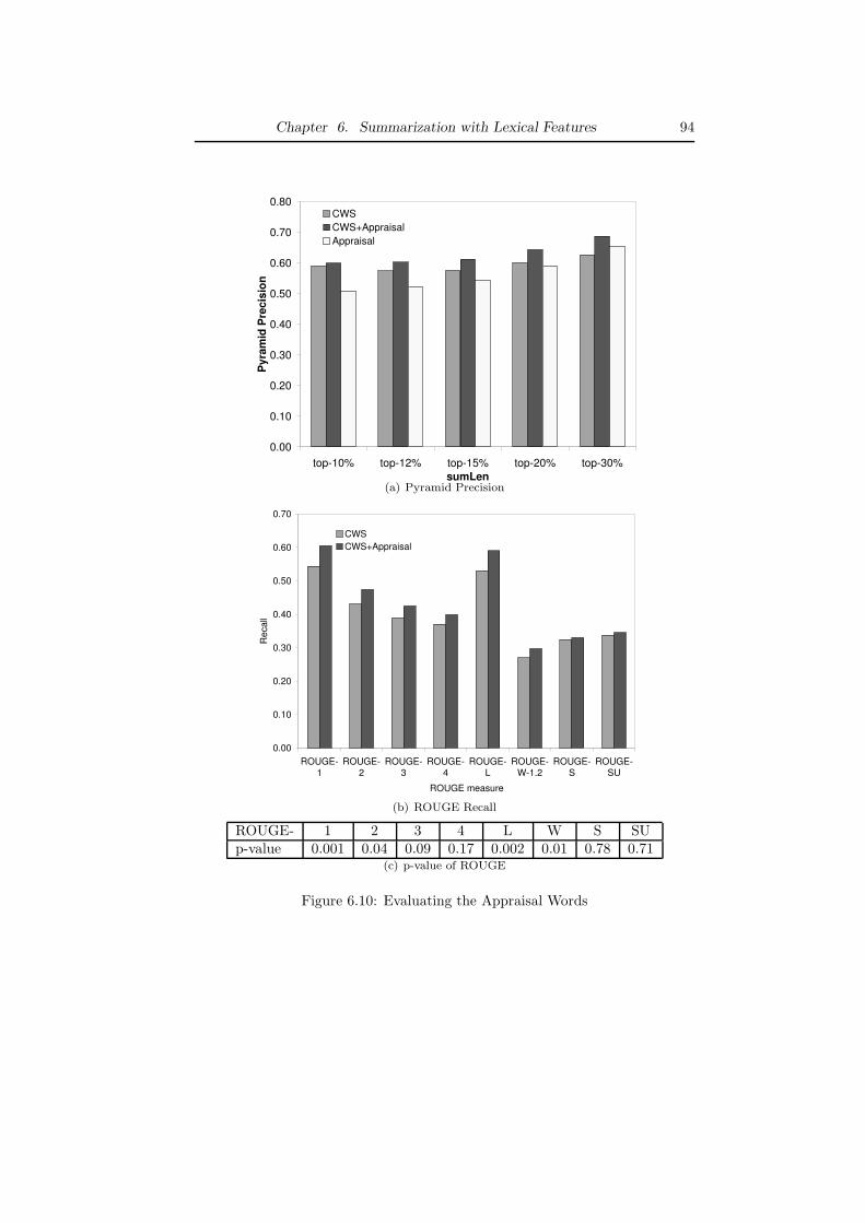
Chapter 6. Summarization with Lexical Features 94
0.00
0.10
0.20
0.30
0.40
0.50
0.60
0.70
0.80
top-10% top-12% top-15% top-20% top-30%
sumLen
Py
ram
id P
rec
isio
n
CWS
CWS+Appraisal
Appraisal
(a) Pyramid Precision
0.00
0.10
0.20
0.30
0.40
0.50
0.60
0.70
ROUGE-
1
ROUGE-
2
ROUGE-
3
ROUGE-
4
ROUGE-
L
ROUGE-
W-1.2
ROUGE-
S
ROUGE-
SU
ROUGE measure
Re
ca
ll
CWS
CWS+Appraisal
(b) ROUGE Recall
ROUGE- 1 2 3 4 L W S SUp-value 0.001 0.04 0.09 0.17 0.002 0.01 0.78 0.71
(c) p-value of ROUGE
Figure 6.10: Evaluating the Appraisal Words

Chapter 6. Summarization with Lexical Features 95
Precision p-valueCWS 0.59 N/ACWS+ComVerb 0.63 0.006CWS+ComNoun 0.62 0.0003CWS+ComAdjv 0.61 0.004CWS+ComAll 0.62 0.0003
Table 6.1: Aggregated Precision and P-value for Communication Words
The next list we experiment on is the opinion bearing words by Kim etal.[32](OpBear). The result is shown in Figure 6.11. From Figure 6.11(a), wecan see that when OpBear is used alone, the precision is lower than, but veryclose to, that of CWS. When integrated with CWS, CWS+OpBear improvesCWS consistently in each summary length. In the summary length of 30%,the improvement is significant with a p-value of 0.05. When aggregated overdifferent summary lengths, CWS+OpBear has a precision of 0.63, which is 0.04higher than that of CWS. This improvement is significant with a p-value of0.006. Figure 6.11(b) compare CWS+OpBear and CWS in ROUGE. From thisfigure we can see that in all ROUGE measures, CWS+OpBear has a higher recallthan that of CWS. In many cases, those improvement is statistically significant,e.g., ROUGE-1, ROUGE-2 and ROUGE-L.
The experiments with three lists of subjective words(OpFind, Appraisal andOpBear) shows that each of the three lists of subjective words can significantlyimprove the accuracy of CWS. Those results support the previous hypothesisthat subjective sentences are important and we can use them for summarizingemail conversations. In terms of runtime, the average runtime for each list is0.2, 0.07, and 0.7 seconds respectively.
Evaluating Communication of Ideas in Roget’s Thesaurus
In this section, we evaluate the three lists obtained from the Roget’s thesaurusand examine whether they can be used to improve CWS. Similar to the previousexperiment, Figures 6.12, 6.13 and 6.14 show the accuracy of using the threelists respectively. Figure 6.12(a), Figure 6.13(a) and Figure 6.14(a) show that allthe three lists improve CWS consistently in pyramid precision in every summarylength. In some cases such improvement is statistically significant even undera single summary length. For example, in Figure 6.12(a) when the summarylength is 30%, the p-value is 0.04. In Figure 6.13(a) when the summary lengthis 15%, 20% and 30%, the p-value is 0.03, 0.04 and 0.02 respectively.
Table 6.1 shows the aggregated precision over all summary length in pyramidprecision. For each method, we also run a 2-tail pairwise student t-test tocompare it with CWS. The result also shows that all three lists can improveCWS statistically significantly. Moreover, CWS+ComVerb obtains the highestprecision among them.

Chapter 6. Summarization with Lexical Features 96
0.00
0.10
0.20
0.30
0.40
0.50
0.60
0.70
0.80
top-10% top-12% top-15% top-20% top-30%
sumLen
Py
ram
id P
rec
isio
n
CWS
CWS+OpBearing
OpBearing
(a) Pyramid Precision
0.00
0.10
0.20
0.30
0.40
0.50
0.60
0.70
ROUGE-
1
ROUGE-
2
ROUGE-
3
ROUGE-
4
ROUGE-
L
ROUGE-
W-1.2
ROUGE-
S
ROUGE-
SU
ROUGE measure
Re
ca
ll
CWS
CWS+OpBear
(b) ROUGE Recall
ROUGE- 1 2 3 4 L W S SUp-value 0.0005 0.02 0.04 0.09 0.0003 0.001 0.30 0.27
(c) p-value of ROUGE
Figure 6.11: Evaluating the List of OpBear

Chapter 6. Summarization with Lexical Features 97
0.00
0.10
0.20
0.30
0.40
0.50
0.60
0.70
0.80
top-10% top-12% top-15% top-20% top-30%
sumLen
Pyra
mid
Pre
cis
ion
CWS
CWS+ComVerb
ComVerb
(a) Pyramid Precision
0.00
0.10
0.20
0.30
0.40
0.50
0.60
0.70
ROUGE-1
ROUGE-2
ROUGE-3
ROUGE-4
ROUGE-L
ROUGE-W-1.2
ROUGE-S
ROUGE-SU
ROUGE measure
Re
ca
ll
CWS
CWS+ComVerb
(b) ROUGE Recall
ROUGE- 1 2 3 4 L W S SUp-value 0.00001 0.00007 0.0009 0.01 0.0001 0.00004 0.93 0.84
(c) p-value of ROUGE
Figure 6.12: Evaluating the ComVerb
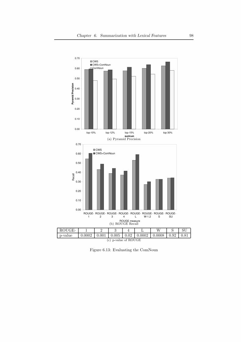
Chapter 6. Summarization with Lexical Features 98
0.00
0.10
0.20
0.30
0.40
0.50
0.60
0.70
top-10% top-12% top-15% top-20% top-30%
sumLen
Pyra
mid
Pre
cis
ion
CWS
CWS+ComNoun
ComNoun
(a) Pyramid Precision
0.00
0.10
0.20
0.30
0.40
0.50
0.60
0.70
ROUGE-
1
ROUGE-
2
ROUGE-
3
ROUGE-
4
ROUGE-
L
ROUGE-
W-1.2
ROUGE-
S
ROUGE-
SU
ROUGE measure
Re
ca
ll
CWS
CWS+ComNoun
(b) ROUGE Recall
ROUGE- 1 2 3 4 L W S SUp-value 0.0002 0.001 0.005 0.02 0.0002 0.0008 0.92 0.81
(c) p-value of ROUGE
Figure 6.13: Evaluating the ComNoun

Chapter 6. Summarization with Lexical Features 99
0.00
0.10
0.20
0.30
0.40
0.50
0.60
0.70
top-10% top-12% top-15% top-20% top-30%
sumLen
Pyra
mid
Pre
cis
ion
CWS
CWS+ComAdjv
ComAdjv
(a) Pyramid Precision
0.00
0.10
0.20
0.30
0.40
0.50
0.60
0.70
ROUGE-
1
ROUGE-
2
ROUGE-
3
ROUGE-
4
ROUGE-
L
ROUGE-
W-1.2
ROUGE-
S
ROUGE-
SU
ROUGE measure
Re
ca
ll
CWS
CWS+ComAdjv
(b) ROUGE Recall
ROUGE- 1 2 3 4 L W S SUp-value 0.00002 0.0002 0.002 0.02 0.00002 0.0001 0.44 0.39
(c) p-value of ROUGE
Figure 6.14: Evaluating the ComAdjv

Chapter 6. Summarization with Lexical Features 100
0.00
0.10
0.20
0.30
0.40
0.50
0.60
0.70
0.80
top-10% top-12% top-15% top-20% top-30%
sumLen
Pyra
mid
Pre
cis
ion
CWS
CWS+ComVerb
CWS+ComNoun
CWS+ComAdjv
CWS+ComAll
(a) Pyramid Precision
Figure 6.15: Evaluating the ComAll
The ROUGE evaluation also gives a consistent result as shown in Figure6.12(b), 6.13(b) and 6.14(b). In all 8 measures of ROUGE, except ROUGE-Sand ROUGE-SU, CWS+Verb, CWS+Noun and CWS+Adjv show statisticallysignificant improvement over CWS. As to the runtime, the average time tocompute the LexCueScore for ComVerb, ComNoun and ComAdjv is 0.04, 0.09and 0.03 respectively, which is almost proportional to their size as well.
Now, after studying the three lists separately, we merge them all togetheras one list ComAll and compare it together with three separate lists discussedabove and CWS. In Figure 6.15 we can see that there is no significant differenceamong these four methods. CWS+ComVerb even works a little better thanCWS+ComAll in terms of the average pyramid precision in many cases.
In this section, we have applied all the proposed approaches to the 20 con-versations from the Enron email dataset. The results have demonstrated thatsubjective words and communication words from Roget’s thesaurus consistentlyand significantly improve CWS. Although cue phrases demonstrate a slight im-provement, it is not comparable to the remaining ones.
6.5.3 Reevaluation with a New Dataset
Dataset and User Study
In the previous experiments, we evaluate the improvement methods proposedin Section 6.2, 6.3 and 6.4 on the 20 conversations. In the following we callthat dataset as Dataset 1. In those experiments on Dataset 1, we showed thatCWS is as accurate as and much more efficient than the method using semantic

Chapter 6. Summarization with Lexical Features 101
Features UserStudy 1 UserStudy 2# of conversations 20 19
# of tree type 15 14# of list type 5 5# emails/conv 5.6 4.5avg sent./conv 37.1 34.4
Table 6.2: Compare Dataset 1 and Dataset 2
distance based on the WordNet. Moreover, by including lexical cues, we canimprove the accuracy of CWS significantly. Besides the effective improvements,there are two unsolved issues in the previous experiments. First, our conclusionsare based on Dataset 1, which is a relatively small dataset containing only 741sentences in 20 conversations. Although many of our discoveries have shownstatistical significance, the dataset may not be large enough to justify the gen-erality of those conclusions. In order to further support those conclusions, it isnecessary to evaluate them with more data. Secondly, some results show con-sistent differences on the average, but their p-values are high, which does notqualify for the statistical significance. One possible reason is the lack of data,which makes it difficult to observe a statistical significance. It is necessary toadd more conversations into the existing dataset and reevaluate the previousconclusions on the whole dataset.
Consequently, we collect another dataset and use it to evaluate differentsummarization approaches. We call this dataset as Dataset 2. Similar to howthe first 20 conversations in Dataset 1 were selected, we select Dataset 2 fromthe largest 10 folders in the Enron dataset. With the same criteria for Dataset1, we also requires that a selected conversation contains at least 4 emails. In thisway, we end up with 19 new conversations. Among them, 5 conversations are achain of emails(based on the email threads), with the remaining ones have a treestructure. Table 6.2 shows a set of quantitative features about both datasets.From this table, we can see that on the average, Dataset 2 and Dataset 1 aresimilar quantitatively, except that on the average a conversation in Dataset 2contains one fewer email than a conversation in Dataset 1.
We also recruit 25 reviewers to “summarize” them. Each conversation isevaluated by 5 reviewers. The given summary length for each conversationis about 30% of the total number of sentences of that conversation, includingboth essential and optional selections. Only one of these 25 reviewers alsoparticipated the user study for Dataset 1. After examining the reviews givenby the reviewers, we identified 4 reviewers who consistently did not follow theexperimental procedure. They selected more essential sentences than the givensummary length, which should include both essential and optional selections.For some reviewers the “essential/given” ratio is as high as 2. Those 4 reviewersdid not understand the experimental procedure. Hence, we replace them byrecruiting another 4 reviewers to generate reviews for the conversations they

Chapter 6. Summarization with Lexical Features 102
MEAD CWSPyramid Precision 0.596 0.597p-value 0.96
Table 6.3: Aggregate Pyramid Precision for MergedDataset
reviewed. We did the same check for the user study on Dataset 1, but no suchreviewers were found. With this user study, we also built a pyramid for theDataset 2 in the same way as we did for the Dataset 1. In the following, we firstevaluate the previous approaches on Dataset 2. Then, we merge Dataset 1 andDataset 2 together and repeat the evaluation on the merged dataset. We callthe merged dataset as MergedDataset.
MEAD and CWS
We first try to compare MEAD and CWS together on Dataset 2 and Merged-Dataset. Figure 6.16(a) shows that when the evaluation is based on the pyra-mid precision, MEAD has a higher precision than that of CWS consistently, butthose differences are not statistically significant. When evaluated by ROUGE,as shown in Figure 6.16(b), CWS is slightly more accurate than MEAD in manycases. This improvement is not significant either. This result is different fromthe result in Chapter 5, where CWS shows significant improvement over MEAD.
We compare the accuracy of either algorithm in Dataset 1 and Dataset 2together. This is shown in Figure 6.17. The x-axis is the summary length andthe y-axis is the pyramid precision. In each summary length, there are four bars,representing the precision of CWS in Dataset 1, CWS in Dataset 2, MEAD inDataset 1 and MEAD in Dataset 2 from the left to the right. From this figurewe can see that under each summary length, CWS has a similar accuracy inboth Dataset 1 and Dataset 2. In contrast, MEAD’s performance varies a lotin two datasets. It has a much higher precision in Dataset 2 than in Dataset 1.CWS shows a stable accuracy. The consistency and stability is a good propertyfor CWS.
We also evaluate CWS and MEAD on MergedDataset and aggregate over allsummary lengths. The average value of CWS and MEAD and the correspondingp-values in Table 6.3 and Table 6.4. From these two tables, we can see that CWSand MEAD have a precision of 0.597 and 0.596 respectively with a p-value of0.96. However, when evaluated in ROUGE the difference is obvious. CWSconsistently works better than MEAD. In ROUGE-S and ROUGE-SU, the p-value is only 0.03.
Semantic Distance in WordNet and Cosine Similarity
Other than CWS, we also examine the performance of the semantic distance inWordNet and the cosine similarity. Figure 6.18 shows that in Dataset 2, neitherCWS-WordNet nor CWS-Cosine can improve CWS, and in some cases their

Chapter 6. Summarization with Lexical Features 103
0.00
0.10
0.20
0.30
0.40
0.50
0.60
0.70
0.80
top-10% top-12% top-15% top-20% top-30%
sumLen
Pyra
mid
Pre
cis
ion
MEAD
CWS
(a) Pyramid Precision
0.00
0.10
0.20
0.30
0.40
0.50
0.60
0.70
ROUGE-
1
ROUGE-
2
ROUGE-
3
ROUGE-
4
ROUGE-
L
ROUGE-
W-1.2
ROUGE-
S
ROUGE-
SU
ROUGE measure
Recall
MEAD
CWS
(b) ROUGE Recall
ROUGE- 1 2 3 4 L W S SUp-value 0.93 0.59 0.97 0.72 0.89 0.22 0.55 0.57
(c) p-value of ROUGE
Figure 6.16: Compare MEAD and CWS in Dataset 2

Chapter 6. Summarization with Lexical Features 104
0.00
0.10
0.20
0.30
0.40
0.50
0.60
0.70
0.80
top-10% top-12% top-15% top-20% top-30%sumLen
Pyra
mid
Pre
cis
ion
CWS-Dataset 1
CWS-Dataset 2
MEAD-Dataset 1
MEAD-Dataset 2
(a) Pyramid Precision
Figure 6.17: Compare CWS and MEAD in Dataset 1 and 2
ROUGE- 1 2 3 4 L W S SUMEAD 0.57 0.45 0.42 0.39 0.56 0.27 0.31 0.32CWS 0.58 0.49 0.44 0.41 0.57 0.29 0.35 0.36p-value 0.42 0.09 0.26 0.26 0.52 0.10 0.03 0.03
Table 6.4: ROUGE Evaluation for MergedDataset

Chapter 6. Summarization with Lexical Features 105
0.00
0.10
0.20
0.30
0.40
0.50
0.60
0.70
top-10% top-12% top-15% top-20% top-30%sumLen
Pre
cis
ion
CWS
CWS-WordNet
CWS-Cosine
Figure 6.18: Dataset 2: Compare CWS, CWS-WordNet and CWS-Cosine
precision is even lower than that of CWS. This result is also consistent with ourprevious conclusions in Dataset 1. When evaluated in MergedDataset, CWSshows significant higher precision(0.60) that that of CWS-WordNet(0.57) witha p-value of 0.04. Thus, the empirical result does not support using WordNeteither from accuracy point of view or from the the efficiency point of view.
Lexical Cues
In the previous experiments on Dataset 1, we have shown that cue phrases,subjective and opinion bearing words can significantly improve the accuracy ofCWS. In this section we re-evaluate this conclusion on Dataset 2.
Table 6.5 shows the average pyramid precision over various summary lengthsand the corresponding p-value versus CWS with a 2-tail pairwise student t-test.Table 6.5 shows that all methods, except CWS+ComAdjv, gain higher precisionthan that of CWS. For CWS+CuePhrase, CWS+Appraisal, CWS+OpBear,CWS+ComVerb and CWS+Noun, the p-value is less than 0.05. CWS+OpFindhas a p-value of 0.06. ComVerb still has the best performance among the 4 listsobtained from Roget’s Thesaurus. Thus, our previous conclusions are still validfor Dataset 2.
Furthermore, we apply those methods on MergedDataset, which is the unionof Dataset 1 and Dataset 2, and compare the performance of different meth-ods pairwise. Table 6.6 shows the average pyramid precision in all datasettogether with the p-value of every pair of methods. The first column and thefirst row are different summarization methods. The second row is the aver-age precision of each method. The pairwise p-values are listed in the corre-sponding cells from the third row to the last row of this table. From this

Chapter 6. Summarization with Lexical Features 106
Methods Average P-value
CWS 0.60 N/ACWS+CuePhrase 0.61 0.04CWS+OpFind 0.64 0.06CWS+Appraisal 0.67 0.002CWS+OpBear 0.65 0.02CWS+ComVerb 0.63 0.0002CWS+ComNoun 0.62 0.05CWS+ComAdjv 0.60 0.87CWS+ComAll 0.61 0.34
Table 6.5: Dataset 2: Aggregated Precision over Various Summary Length andP-value
table, we see that CWS+OpFind has the greatest precision among all methods.Meanwhile, it is statistically significantly better than all remaining methods ex-cept CWS+Appraisal and CWS+OpBear. CWS+Appraisal and CWS+OpBearhas a similar performance, where the average is the same and they are signif-icantly better than the other methods except CWS+OpFind, CWS+Verb andCWS+Noun. Among the remaining lists, ComVerb and ComNoun shows sim-ilar performance. However, CWS+ComVerb has significant improvement overMEAD, while CWS+Noun cannot. Consequently, through the empirical eval-uation, we find that the subjective word list OpFind has the best performanceamong all lexical cues.
Having shown that subjective words and words for communication of ideascan improve CWS significantly, an interesting question to ask is that whetherthose methods can also improve over MEAD. We use the same way describedin Equation 6.12, For each sentence, we use the MEADScore plus the Lex-CueScore as the sentence score and rank all sentences in a conversation basedon this integrated score. Table 6.7 shows the average pyramid precision on theMergedDataset together with the corresponding p-values between each inte-grated method and MEAD. From this table, we can see that none of the lexicalcues we have tried can improve MEAD in the same way as they do for CWS. Insome cases, the integrated version even significantly decrease the precision, e.g.,MEAD+CuePhrase and MEAD+Appraisal. One may be curious about whylexical cues can significantly improve CWS but not MEAD. In a more detailedanalysis, we find that MEAD+LEXLIST have different performance in Dataset1 and Dataset 2. In Dataset 1, MEAD+LEXLIST can improve MEAD to aprecision that is a little lower than that of CWS alone. However, in Dataset 2,MEAD+LEXLIST significantly decreases the precision to that of CWS or evenlower. This also supports our previous analysis of MEAD’s instability in differ-ent datasets. Consequently, this result strengthens the previous conclusion thatintegrating CWS together with lexical cues, especially subjective cues, have ahigher accuracy.
Chapter 6. Summarization with Lexical Features 107
6.6 Summary
In this chapter, we study several lexical approaches to improve CWS. First,we build a sentence quotation graph to represent the conversation structure inthe sentence granularity. This sentence quotation graph unifies the previousClueWordSummarizer(CWS) and the methods discussed in this chapter.
Second, we extend the concept of clue words by considering not only wordswith the same stem but also synonyms, antonyms or words with semanticallysimilar meaning. We use the semantic similarity based on the well-known Word-Net. The empirical results show that CWS is not inferior to the more sophisti-cated semantic similarity.
Third, we tried several sentence-based lexical cues. The experimental re-sults show that sentences with subjective opinions also play an important rolefor email summarization. Among the lists of subjective words we have tried,OpFind obtains the highest accuracy. Additionally, words about communica-tion of ideas from the Roget’s Thesaurus also improve CWS, especially theverbs. But its improvement is not as significant as that of OpFind. The suc-cess of ComVerb also indicates that POS could make a difference as to emailsummarization. This can be explored further in the future.

Chapter
6.
Sum
mariza
tion
with
Lex
icalFea
tures
108
CWS+ MEAD CWS CuePh Appr OpFind OpBear ComVerb ComNoun ComAdjv ComAll
avg 0.60 0.60 0.61 0.64 0.65 0.64 0.63 0.62 0.603 0.62
MEAD x 0.96 0.52 0.01 0.0001 0.001 0.05 0.13 0.67 0.24CWS x 0.02 0.0004 0.0000 0.0007 0.00 0.0004 0.03 0.004CWS+CuePh x 0.003 0.0003 0.003 0.003 0.02 0.55 0.16CWS+Appr x 0.12 0.59 0.35 0.16 0.004 0.05CWS+OpFind x 0.25 0.05 0.01 0.0004 0.002CWS+OpBear x 0.20 0.09 0.01 0.02CWS+ComVerb x 0.46 0.002 0.14CWS+ComNoun x 0.01 0.19CWS+ComAdjv x 0.05CWS+ComAll x
Table 6.6: Integrate CWS with Lexical Cues in MergedDataset
MEAD+ MEAD CuePh Appr OpFind OpBear ComVerb ComNoun ComAdjv ComAll
avg 0.60 0.56 0.58 0.61 0.60 0.55 0.58 0.53 0.57
p-value(MEAD) x 0.02 0.16 0.15 0.7 0.01 0.47 0.0001 0.14
Table 6.7: Integrate MEAD with Lexical Cues in MergedDataset

109
Chapter 7
Conclusions and Future
Work
7.1 Conclusions
In this thesis, we study how to discover and summarize email conversations. Wefirst develop a framework to identify and regenerate hidden emails and proposeseveral optimization methods to improve the runtime performance. We alsobuild a fragment quotation graph and a sentence quotation graph to representthe email conversation structure, in which the hidden emails are included aswell. Based on the fragment/sentence quotation graph, we propose a novelemail summarization approach, ClueWordSummarizer(CWS) and improve itwith lexical feature, e.g., cue phrases and subjective words. Specifically, thecontributions of this thesis can be summarized as follows.
• We study the hidden email problem, which is very important for emailsummarization and other applications but has been largely omitted inthe previous research on emails. Our user study for email summarizationshows that many important sentences evaluated by human summarizersare from hidden emails.
• To discover and regenerate hidden emails, we propose a framework: Hid-denEmailFinder. In this framework, we build a precedence graph to rep-resent the relative textual orderings among hidden fragments belonging tothe same hidden email. Then, we propose the bulletized email model torepresent the partial orderings among hidden fragments. A key technicalresult is that we give a necessary and sufficient condition for a hiddenemail be exactly regenerated as one single bulletized email. We also givean algorithm that guarantees to generate the correct bulletized hiddenemails if the necessary and sufficient condition is satisfied. Two heuristicsare also developed to deal with cases when the condition is not satisfied.
We also study two optimization approaches to improve the runtime per-formance of HiddenEmailFinder when dealing with large folders and longemails. Both approaches are based on word indexing to reduce the num-ber of comparisons to discover hidden fragments. We give conditions thatguarantee no decrease of the accuracy.
The framework of HiddenEmailFinder can also be applied to the emailforensic and email mining applications, where discovering information

Chapter 7. Conclusions and Future Work 110
from emails is crucial for the investigators. Specifically, it can be usedfor extracting email conversations from an email folder with some minorchanges.
One important contribution is the empirical study with the Enron dataset.The results not only show the prevalence of hidden emails but also demon-strate that our framework is accurate and the optimization methods areeffective and scalable to large folders.
• We build a fragment quotation graph to capture the email conversations.The fragment quotation graph is able to capture the conversation struc-ture in selective quotations and represent the email conversations withfiner granularity than the commonly used email thread. Furthermore, wedevelop a sentence quotation graph to represent the conversation in thesentence level. The sentence quotation graph is based on the fragmentquotation graph, but is more flexible and easy to use for summarizationwith sentence extraction.
• With the fragment/sentence quotation graph representing the email con-versation structure, we develop an email summarizer, ClueWordSumma-rizer(CWS), which relies on a novel concept, the clue word. Clue wordsare based on the conversation structure and capture the cohesion withinthe conversation.
• We compare CWS with one state-of-the-art email summarization methodand one generic multi-document summarization method. Two commonlyused evaluation metrics are applied. One is the pyramid precision, and theother is ROUGE. Our experiments with the Enron email dataset show thatCWS can generate more accurate summaries when compared with othermethods.
• We also explore many ways to improve CWS. One important discovery isthat words expressing subjective opinions can significantly improve CWS.Note that most of the email conversations in the Enron dataset are dis-cussing some business issues related to the ex-Enron corporation. Many ofthose conversations contain opinions of the authors in the discussion. Ourdiscovery clearly indicates that subjective opinions are very important forsuch email conversations.
7.2 Future Work
Discovering and summarizing email conversations is a relatively new but impor-tant topic that has not been studied extensively. Besides the work presentedin this thesis, in the future we would like to further explore in the followingdirections.

Chapter 7. Conclusions and Future Work 111
• We have shown that hidden emails are very important for email summa-rization since they can contain crucial information. Besides email summa-rization, we would like to explore how hidden emails affects other appli-cations, e.g., email forensic and email visualization.
• Other than the fragment/sentence quotation graph, we want to furtherexplore how to capture the conversation structure. Although in this the-sis we have shown that semantic distance based on the WordNet doesnot work better than the simple clue words based on stems, we want tostudy other measures of semantic distance based on the WordNet and thequotation graph.
• Our experiments indicate that subjective words are of great importancefor summarizing email conversations. In this thesis, we only adopt thesubjective words discovered by other researchers and use them in a straightforward way by summing up their frequency in a sentence. In the future,we would like to study how to identify subjective words and sentencesin email conversations directly. Moreover, it is also interesting to findwhether the polarity(positive or negative) of a sentence can affect thesummary accuracy or not, e.g., whether or not the negative opinions aremore important than the positive ones.
• Email conversations are discussions among a group of people. The author’ssocial role can also affect the importance of the email. It is interesting toknow whether we can further improve email summarization by includingthe social network analysis obtained from the user’s email folders.
• In this thesis, the email conversations are chosen from the Enron emaildataset. Most of them are discussions related to the business issues ofthe ex-Enron corporation. We want to study how well our summarizationapproaches work for other types of email conversations. Meanwhile, theautomatic classification of email conversations in different types may alsobe interesting for the purpose of summarization.
• In this thesis, we only study the accuracy of email summaries withoutconsidering how to present the summary to the user. In the future wewant to study this further, e.g., the bulletized email model could be usedto present an email summary.
• Finally, the current summarization methods are producing informativesummaries, i.e., the summary covers the crucial information in the orig-inal conversation. By reading the summary, a user is not supposed toread the original emails again in most cases. However, indicative sum-mary can also be very useful. For example, when a user is searching fora specific conversation or email, a short indicative summary about theemail(conversation) can be helpful for the user to decide whether to readit or not. This is also related to question-answering for emails. We planto explore all these issues in the future.

112
Bibliography
[1] Rakesh Agrawal, Sridhar Rajagopalan, Ramakrishnan Srikant, and YirongXu. Mining newsgroups using networks arising from social behavior. InWWW ’03: Proceedings of the 12th International Conference on WorldWide Web, pages 529–535, 2003.
[2] Regina Barzilay and Michael Elhadad. Using lexical chains for text sum-marization. In Proceedings of the Intelligent Scalable Text SummarizationWorkshop (ISTS’97) ACL, 1997.
[3] Regina Barzilay, Kathleen R. McKeown, and Michael Elhadad. Informationfusion in the context of multi-document summarization. In Proceedings ofthe 37th annual meeting of the Association for Computational Linguisticson Computational Linguistics, pages 550–557. Association for Computa-tional Linguistics, 1999.
[4] Giuseppe Carenini, Raymond T. Ng, and Adam Pauls. Interactive multi-media summaries of evaluative text. In IUI ’06: Proceedings of the 11thinternational conference on Intelligent user interfaces, pages 124–131, NewYork, NY, USA, 2006. ACM.
[5] Giuseppe Carenini, Raymond T. Ng, and Adam Pauls. Multi-documentsummarization of evaluative text. In Proceedings of the 11st Conferenceof the European Chapter of the Association for Computational Linguistics,Trento, Italy, April 3-7 2006.
[6] Giuseppe Carenini, Raymond T. Ng, and Ed Zwart. Extracting knowledgefrom evaluative text. In Proceedings of the 3rd International Conferenceon Knowledge Capture (K-CAP 2005), pages 11–18, October 2-5 2005.
[7] Vitor R. Carvalho and William W. Cohen. Learning to extract signatureand reply lines from email. In First Conferences on Emails and Anti-spam,2004.
[8] Li-Te Cheng and Daniel Gruen. A mobile user interface for threading,marking, and previewing email. In IBM Technical Report 2003-08, 2003.
[9] US Federal Energy Regulatory Commission.http://www.ferc.gov/industries/electric/indus-act/wem/pa02-2/info-release.asp.

Bibliography 113
[10] Simon Corston-Oliver, Eric K. Ringger, Michael Gamon, and RichardCampbell. Integration of email and task lists. In First Conference onEmail and Anti-Spam, Mountain View, California, USA, July 30-31 2004.
[11] Hoa Trang Dang. Overview of duc 2005. In Proceedings of the DocumentUnderstanding Conference (DUC’05), Vancouver, B.C., Canada, October9-10 2005.
[12] Hoa Trang Dang. Overview of duc 2006. In Proceedings of the DocumentUnderstanding Conference (DUC’06), New York, USA, June 8-9 2006.
[13] Milind Dawande, Pinar Keskinocak, Jayashankar M. Swaminathan, andSridhar Tayur. On bipartite and multipartite clique problems. Journal ofAlgorithms, 41(2):388–403, 2001.
[14] Chris Schmandt Derek Lam, Steven L. Rohall and Mia K. Stern. Exploitinge-mail structure to improve summarization. In CSCW’02 Poster Session,2002.
[15] Nicolas Ducheneaut and Victoria Bellotti. E-mail as habitat: an explorationof embedded personal information management. Interactions, 8(5):30–38,2001.
[16] Jack Edmonds and Richard M. Karp. Theoretical improvements in algo-rithmic efficiency for network flow problems. J. ACM, 19(2):248–264, 1972.
[17] H. P. Edmundson. New methods in automatic extracting. Journal of theAssociation for Computing Machinery, 16(2):264–285, April 1969.
[18] Gunes Erkan and Dragomir R. Radev. Lexrank: graph-based lexical cen-trality as salience in text summarization. Journal of Artificial IntelligenceResearch(JAIR), 22:457–479, 2004.
[19] Andrea Esuli and Fabrizio Sebastiani. Sentiwordnet: A publicly availablelexical resource for opinion mining. In Proceedings of the InternationalConference on Language Resources and Evaluation, May 24-26 2006.
[20] Robert Farrell, Peter G. Fairweather, and Kathleen Snyder. Summarizationof discussion groups. In Proceedings of the tenth international conferenceon Information and knowledge management, pages 532–534, 2001.
[21] Christiane Fellbaum(Editor). WordNet: An Electronic Lexical Database.The MIT Press, Cambridge, MA, 1998.
[22] Danyel Fisher and Paul Moody. Studies of automated collection of emailrecords. In University of Irvine ISR Technical Report UCI-ISR-02-4.
[23] George Forman, Kave Eshghi, and Stephane Chiocchetti. Finding similarfiles in large document repositories. In KDD ’05: Proceeding of the eleventhACM SIGKDD international conference on Knowledge discovery in datamining, pages 394–400, 2005.

Bibliography 114
[24] A. Resnick G. J. Rath and T. R. Savage. The formation of abstracts by theselection of sentences: Part 1: Sentence selection by man and machines. InAmerican Documentation, volume 12(2), pages 139–141, 1961.
[25] Jade Goldstein, Mark Kantrowitz, Vibhu O. Mittal, and Jamie G. Car-bonell. Summarizing text documents: sentence selection and evaluationmetrics. In Research and Development in Information Retrieval, pages121–128, Berkeley, California, 1999.
[26] Jade Goldstein, Vibhu O. Mittal, Jamie Carbonell, and Mark Kantrowitz.Multi-document summarization by sentence extraction. In Udo Hahn,Chin-Yew Lin, Inderjeet Mani, and Dragomir R. Radev, editors,ANLP/NAACL’00-WS, Seattle, WA, April 2000.
[27] Douglas J. Hermann and Lise S. Rubenfeld. Journal of PsycholinguisticResearch, 14(1), January 1985.
[28] Dorit S. Hochbaum. Approximating clique and biclique problems. Journalof Algorithms, 29(1):174–200, 1998.
[29] Eduard H. Hovy and Yigal Arens. Automatic generation of formatted text.In AAAI, pages 92–97, 1991.
[30] Aaron Harnly Jen-Yuan Yeh. Email thread reassembly using similaritymatching. In Third Conference on Email and Anti-Spam (CEAS), July 27- 28 2006.
[31] Jason J. Jung and GeunSik Jo. Template-based e-mail summarization forwireless devices. In Proceedings of the 18th International Symposium onComputer and Information Sciences(ISCIS’03), volume 2869 of LectureNotes in Computer Science, pages 99–106. Springer, November 3-5 2003.
[32] Soo-Min Kim and Eduard Hovy. Automatic detection of opinion bearingwords and sentences. In Proceedings of the Second International Joint Con-ference on Natural Language Processing: Companion Volume, Jeju Island,Republic of Korea, October 11-13 2005.
[33] Soo-Min Kim and Eduard Hovy. Identifying and analyzing judgment opin-ions. In Proceedings of the main conference on Human Language TechnologyConference of the North American Chapter of the Association of Computa-tional Linguistics, pages 200–207, Morristown, NJ, USA, 2006. Associationfor Computational Linguistics.
[34] Bryan Klimt and Yiming Yang. The enron corpus: a new dataset for emailclassification research. In 15th European Conference on Machine Learning(ECML), pages 217–226, September 20-24 2004.
[35] Kevin Knight and Daniel Marcu. Summarization beyond sentence extrac-tion: a probabilistic approach to sentence compression. Artificial Intelli-gence, 139(1):91–107, 2002.

Bibliography 115
[36] Alistair Knott. A data-driven methodology for motivating a set of coherencerelations. PhD thesis, 1996.
[37] David D. Lewis and K. A. Knowles. Threading electronic mail - a pre-liminary study. Information Processing and Management, 33(2):209–217,1997.
[38] Chin-Yew Lin. Rouge: A package for automatic evaluation of summaries. InProceedings of the ACL Text Summarization Workshop., Barcelona, Spain,2004.
[39] Dekang Lin. Book reviews: Wordnet: an electronic lexical database. Com-putational Linguistics, 25, June 1999.
[40] H. P. Luhn. The automatic creation of literature abstracts. IBM Journalof Research Development, 2(2):159–165, 1958.
[41] Inderjeet Mani. Recent developments in text summarization. In Proceed-ings of the 10th International Conference on Information and KnowledgeManagement, pages 529–531, Atlanta, Georgia, USA, 2001.
[42] Daniel Marcu. From discourse structures to text summaries. In Proceedingsof the 14th National Conference on Artificial Intelligence (AAAI-97), pages629–636, Providence, Rhode Island, 1997. AAAI Press / MIT Press.
[43] Kathleen McKeown, Regina Barzilay, Sasha Blair-Goldensohn, DavidEvans, Vasileios Hatzivassiloglou, Judith Klavans, Ani Nenkova, BarrySchiffman, and Sergey Sigelman. The Columbia multi-document summa-rizer. In DUC’02-WS, Philadelphia, PA, July 2002.
[44] Kathleen R. McKeown, Vasileios Hatzivassiloglou, Regina Barzilay, BarrySchiffman, David Evans, and Simone Teufel. Columbia multi-documentsummarization: approach and evaluation. In Proceedings of the DocumentUnderstanding Conference 2001, 2001.
[45] Kathleen R. McKeown, Judith Klavans, Vasileios Hatzivassiloglou, ReginaBarzilay, and Eleazar Eskin. Towards multidocument summarization byreformulation: progress and prospects. In AAAI’99, pages 453–460, July18–22 1999.
[46] Gabriel Murray, Steve Renals, Jean Carletta, and Johanna Moore. In-corporating speaker and discourse features into speech summarization. InProceedings of the main conference on Human Language Technology Con-ference of the North American Chapter of the Association of ComputationalLinguistics, pages 367–374, Morristown, NJ, USA, 2006. Association forComputational Linguistics.
[47] Ani Nenkova, Rebecca Passonneau, and Kathleen McKeown. The pyramidmethod: incorporating human content selection variation in summarizationevaluation. ACM Transaction on Speech and Language Processing, 4(2):4,2007.

Bibliography 116
[48] Paula S. Newman. Exploring discussion lists: steps and directions. In Pro-ceedings of the second ACM/IEEE-CS joint conference on Digital libraries,pages 126–134, 2002.
[49] Paula S. Newman and John C. Blitzer. Summarizing archived discussions:a beginning. In IUI ’03: Proceedings of the 8th international conferenceon Intelligent user interfaces, pages 273–276, New York, NY, USA, 2003.ACM Press.
[50] Paul Over and James Yen. An introduction to duc 2004 intrinsic evaluationof generic new text summarization systems. In Proceedings of the DocumentUnderstanding Conference (DUC’04), Boston, USA, May 6-7 2004.
[51] D. B. Skillicorn P. S. Keila. Structure in the enron email dataset. Com-putational and Mathematical Organization Theory, 11(3):183 – 199, Oct2005.
[52] Bo Pang and Lillian Lee. A sentimental education: sentiment analysisusing subjectivity summarization based on minimum cuts. In ACL ’04:Proceedings of the 42nd Annual Meeting on Association for ComputationalLinguistics, page 271, Morristown, NJ, USA, 2004. Association for Com-putational Linguistics.
[53] Rene Peeters. The maximum edge biclique problem is np-complete. Dis-crete Appl. Math., 131(3):651–654, 2003.
[54] John C. Platt. Fast training of support vector machines using sequen-tial minimal optimization. In Advances in kernel methods: support vectorlearning, pages 185–208, Cambridge, MA, USA, 1999. MIT Press.
[55] Dragomir R. Radev, Hongyan Jing, and Malgorzata Budzikowska.Centroid-based summarization of multiple documents: sentence extraction,utility-based evaluation, and user studies. In NAACL-ANLP 2000 Work-shop on Automatic summarization, pages 21–30, Morristown, NJ, USA,2000. Association for Computational Linguistics.
[56] Dragomir R. Radev, Hongyan Jing, Malgorzata Stys, and Daniel Tam.Centroid-based summarization of multiple documents. Information Pro-cessing and Management, 40(6):919–938, November 2004.
[57] Owen Rambow, Lokesh Shrestha, John Chen, and Chirsty Lauridsen. Sum-marizing email threads. In HLT/NAACL, May 2–7 2004.
[58] Lance Ramshaw and Mitch Marcus. Text chunking using transformation-based learning. In Proceedings of the Third Workshop on Very Large Cor-pora, pages 82–94. Association for Computational Linguistics, 1995.
[59] Ellen Riloff and Janyce Wiebe. Learning extraction patterns for subjectiveexpressions. In Proceedings of the 2003 conference on Empirical methods innatural language processing, pages 105–112, Morristown, NJ, USA, 2003.Association for Computational Linguistics.

Bibliography 117
[60] Peter Mark Roget. Roget’s thesaurus of english words and phrases. Inhttp://www.gutenberg.org/etext/10681.
[61] Steven L. Rohall, Dan Gruen, Paul Moody, Martin Wattenberg, Mia Stern,Bernard Kerr, Bob Stachel, Kushal Dave, Robert Armes, and Eric Wilcox.Remail: a reinvented email prototype. In CHI Extended Abstracts, pages791–792, 2004.
[62] Gerard Salton, Amit Singhal, Mandar Mitra, and Chris Buckley. Auto-matic text structuring and summarization. Information Processing andManagement: an International Journal, 33(2):193–207, 1997.
[63] Shlomo Hershkop Salvatore J. Stolfo. Email mining toolkit supporting lawenforcement forensic analyses. In DG.O, pages 221–222. Digital Govern-ment Research Center, 2005.
[64] Barry Schiffman, Ani Nenkova, and Kathleen McKeown. Experiments inmultidocument summarization. In Proceedings of the second internationalconference on Human Language Technology Research, pages 52–58, SanFrancisco, CA, USA, 2002. Morgan Kaufmann Publishers Inc.
[65] Kulesh Shanmugasundaram and Nasir D. Memon. Automatic reassemblyof document fragments via context based statistical models. In 19th AnnualComputer Security Applications Conference (ACSAC 2003), December 8 -12 2003.
[66] Andrea Esuli Shlomo Argamon, Kenneth Bloom and Fabrizio Sebastiani.Automatically determining attitude type and force for sentiment analysis.In Proceedings of the 3rd Language and Technology Conference, pages 369–373, October 5-7 2007.
[67] Lokesh Shrestha and Kathleen McKeown. Detection of question-answerpairs in email conversations. In Proceedings of COLING’04, pages 889–895, August 23–27 2004.
[68] Satanjeev Banerjee Siddharth Patwardhan and Ted Pedersen. Using mea-sures of semantic relatedness for word sense disambiguation. In Proceedingsof the Fourth International Conference on Intelligent Text Processing andComputational Linguistics, pages 241–257, February 2003.
[69] H. Gregory Silber and Kathleen F. McCoy. Efficient text summarizationusing lexical chains. In IUI ’00: Proceedings of the 5th international con-ference on Intelligent user interfaces, pages 252–255. ACM, 2000.
[70] Evelyne Tzoukermann Smaranda Muresan and Judith L. Klavans. Com-bining linguistic and machine learning techniques for email summarization.In Walter Daelemans and Remi Zajac, editors, Proceedings of CoNLL-2001,pages 152–159. Toulouse, France, 2001.

Bibliography 118
[71] Erkki Sutinen and Jorma Tarhio. Filtration with q-samples in approxi-mate string matching. In CPM ’96: Proceedings of the 7th Annual Sympo-sium on Combinatorial Pattern Matching, pages 50–63, London, UK, 1996.Springer-Verlag.
[72] Jie Tang, Hang Li, Yunbo Cao, and ZhaoHui Tang. Email data cleaning.In ACM SIGKDD’05, pages 489–498, 2005.
[73] Siddharth Patwardhan Ted Pedersen and Jason Michelizzi. Word-net::similarity - measuring the relatedness of concepts. In Proceedings ofFifth Annual Meeting of the North American Chapter of the Associationfor Computational Linguistics (NAACL-04), pages 38–41, May 3-5 2004.
[74] Evelyne Tzoukermann, Smaranda Muresan, and Judith L. Klavans. Gist-it: summarizing email using linguistic knowledge and machine learning. InWalter Daelemans and Remi Zajac, editors, Proceedings of HLT/KM 2001Workshop at ACL/EACL 2001 Confenrence. Toulouse, France, 2001.
[75] V. Vapnik. The nature of statistical learning theory. Springer-Verlag, NewYork, 1995.
[76] Gina Danielle Venolia and Carman Neustaedter. Understanding sequenceand reply relationships within email conversations: a mixed-model visu-alization. In CHI ’03: Proceedings of the SIGCHI conference on Humanfactors in computing systems, pages 361–368, 2003.
[77] Stephen Wan and Kathleen McKeown. Generating overview summariesof ongoing email thread discussions. In Proceedings of COLING’04, the20th International Conference on Computational Linguistics, August 23–27 2004.
[78] Michael White, Tanya Korelsky, Claire Cardie, Vincent Ng, David Pierce,and Kiri Wagstaff. Multidocument summarization via information extrac-tion. In HLT ’01: Proceedings of the first international conference on Hu-man language technology research, pages 1–7, Morristown, NJ, USA, 2001.Association for Computational Linguistics.
[79] Steve Whittaker and Candace Sidner. Email overload: exploring personalinformation management of email. In CHI ’96: Proceedings of the SIGCHIconference on Human factors in computing systems, pages 276–283, 1996.
[80] Theresa Wilson, Paul Hoffmann, Swapna Somasundaran, Jason Kessler,Janyce Wiebe, Yejin Choi, Claire Cardie, Ellen Riloff, and Siddharth Pat-wardhan. Opinionfinder: a system for subjectivity analysis. In Proceedingsof HLT/EMNLP on Interactive Demonstrations, pages 34–35, Morristown,NJ, USA, 2005. Association for Computational Linguistics.
[81] Theresa Wilson, Janyce Wiebe, and Paul Hoffmann. Recognizing contex-tual polarity in phrase-level sentiment analysis. In HLT ’05: Proceedings of
Bibliography 119
the conference on Human Language Technology and Empirical Methods inNatural Language Processing, pages 347–354, Morristown, NJ, USA, 2005.Association for Computational Linguistics.
[82] Jianwu Yang Xiaojun Wan and Jianguo Xiao. Towards an iterative re-inforcement approach for simultaneous document summarization and key-word extraction. In Proceedings of the 45th Annual Meeting of the Associa-tion of Computational Linguistics, pages 552–559, Prague, Czech Republic,June 2007. Association for Computational Linguistics.
[83] Xifeng Yan, Philip S. Yu, and Jiawei Han. Substructure similarity search ingraph databases. In SIGMOD ’05: Proceedings of the 2005 ACM SIGMODinternational conference on Management of data, pages 766–777, New York,NY, USA, 2005. ACM Press.

120
Appendix A
Proof of Theorem 1
THEOREM 1 A weakly connected precedence graph G can be represented by asingle bulletized email with every edge captured and no inclusion of spuriousedges, iff G is a strict and complete parent-child graph.ProofSufficiency: if G is a strict and complete parent-child graph ⇒ G can be rep-resented as a document dG
s2 sns1 ... ...
... ...
... ... ... ...
.........
.........UmU1
VmV1
G
V
U
G’
...
...
V’
(a) Base Case: length = 0
(a) Inductive Case: length = k+1
Figure A.1: Proof for Sufficiency
Let G.length denote the maximum path length in G.
1. G.length = 0This is the base case where G consists of a set of disconnected nodess1, . . . , sn. Thus, G can be represented as [{s1, s2, ..., st}], t ≥ 1.
2. G.length ≤ kSuppose all graph G with G.depth ≤ k can be represented as a documentd.
3. G.length = k + 1Given a graph with G.length = k + 1, let V denote all the leaves in G,Ev denote all edges incident with V . We create a subgraph G′ ⊂ G byremoving V and Ev from G. Let U denote all the leaves in G′. In the

Appendix A. Proof of Theorem 1 121
x
u’
v’v
y
u
Figure A.2: Formation of V and U
following, we first prove that G′ is also a strict and complete parent-childgraph.
∀(x, v) ∈ Ev, if x 6∈ U , then v does not have a parent in U , i.e., parent(v)∩U = ∅. As shown in Figure A.2, for any edge (x, v′) ∈ Ev and x 6∈ U ,there exists at least one leave u′ ∈ U , which is a descendant of x. Sinceu′ 6∈ V , there exists a node v′ ∈ V which is a child of u′. Since G is aminimum equivalent graph(MEG), v 6= v′.
Supposed v has a parent u ∈ U , nodes u, v, x and y ∈ child(x) and y isthe ancestor of v′ constitute a parent-child graph. Due to the requirementof completeness, there must be an edge (u, y). This contradicts with thefact that u is a leave because y 6∈ V . Hence, we conclude that V can bedivided into two subsets V = Vu ∪ V ′ and Vu ∩ V ′ = ∅, s.t., parent(Vu) =U, parent(V ′) ∩ U = ∅.
Suppose U and Vu constitute m parent-child subgraphs: PCi = (Ui, Vi, Ei), i ∈[1, m]. U1∪U2∪. . .∪Um = U and V1∪V2∪. . .∪Vm = V . Removing Vu andthe corresponding nodes in Ev from G does not bring in any non-strictnessand incompleteness.
Suppose V ′ is involved in h parent-child subgraphs, i.e., PCj = (Pj , Cj , Ej), j ∈[1, h]. In this way, V ′ is partitioned into h non-overlapping sets as V ′ ={V ′
1 , V ′2 , . . . , V ′
h}, Vj ⊆ Cj , j ∈ [1, h]. Since G is a complete parent-childgraph, every PCj is a biclique. Removing V ′ and all the correspond-ing edges does not bring in any incompleteness nor non-strictness either.Consequently, G′ is also a strict and complete parent-child graph.
Since the longest path in G must terminate at a node in V , G′.length = k.Hence, G′ can be represented by document dG′ = [d′1; d
′2; ...; d
′n]. d′i, i ∈
[1, n] is either a single document or a set of documents d′i = {d′i1 , ..., d′ipi
}.
It is obvious that all nodes in U are in d′n because they are leaves in G′.In the following, we show that we can generate a new document dG basedon dG′ , which exactly represents G. We first show how we add VU intodG′ , and then show how we add V ′.
Add nodes in V . Without loss of generality, we prove that V1 can beadded into dG′ correctly as shown in Figure A.3(a).

Appendix A. Proof of Theorem 1 122
TG
CV’1
... ...
X
Cv
... ...
C’v
Cm
Pm
... ...
Uj
Vj
... ...
... ...
... ...
X
U1
V’1
(a) Adding V
... ...
t
y
V1
U1
... ...
... ...
... ...
(b) Adding V’
... ...
t
y
GT’1
P’1
C’1
Vj
Figure A.3: Adding Nodes into dG′
Let PCB denote the set of all parent-child subgraphs which precede bothV1 and at least one nodes in Vj , j ∈ [2, m]. For each parent-child sub-graph PC = (P, C, E), we define the maximum depth of the nodes in theparent set P as the depth of this parent-child subgraph. Let PCM =(Pm, Cm, Em) denote the parent-child subgraph with maximum depth inPCB . Thus, all nodes in Pm and a subset of Cm are ancestors of V1.Let Cv denote all V1’s ancestors in Cm, and let T denote the union of Cv
and all its descendants in G′. Thus, for every node t ∈ T , we have thefollowing two conclusions:(1) t is an ancestor of V1, and does not precede any leaf not in V1. Oth-erwise, t is in a parent-child subgraph whose depth is higher than that ofPCM .(2) parent(t) are descendants of Pm. Suppose there exists a node y ∈parent(t) and y is not a descendant of Pm as shown in Figure A.3. Ac-cording to the requirement of strictness, all nodes in Pm and Cm precedest, and hence precedes V1. This contradicts with the previous conditionthat C′
v are not ancestors of V1.
Consequently, for every parent-child subgraph, which precedes V1 and doesnot precede any leaf in Vj , j ∈ [2, m], the parent and child sets are bothsubsets of T .
Thus, all the nodes of T induce a subgraph GT of G′. It is obvious that

Appendix A. Proof of Theorem 1 123
GT is also a complete and strict parent-child graph. Otherwise, G′ is nota strict and complete parent-child graph. The depth of GT is less than k.Thus, there exists a document dGt
which represents GT . Since GT is onlyconnected with Pm and its ancestors, dGt
can be represented in dG′ as[. . . ; {[dGT
], . . .}]. Hence, we can add V1 as follows: [. . . ; {[dGT; V1], . . .}].
Thus, we only include the ordering between leaves in GT and V1, i.e., theedge set E1 in PC1 = (U1, V1, E1).
Add nodes in V’. Secondly, we prove that V ′ can be to document dG′
correctly. Without loss of generality, we show how V ′1 is added as shown
in Figure A.3(b).
After removing V ′ from G, the child set C′1 in PC′
1 = (P ′1, C
′1, E
′1) contains
at least one node not in C′1. Otherwise P ′
1 are leaves in G′. Hence, PC′1
still exists as PC′1 = (P ′
1, C′V ′
1, E′
1), where C′V ′
1= C′
1 − V ′1 .
Moreover, we prove that for any descendant t of C′V ′
1, all its parents are
descendants of P ′1. Suppose there is a node y ∈ parent(t), s.t., y is not
a descendant of P ′1. Due to strictness, the node sets P ′
1, C′V ′
1and V ′
1 all
precedes t. But this contradicts with the fact that V ′1 are the leaves in G.
Thus, all parents of t are descendant of P ′1.
Let T ′1 denote all the descendants of P ′
1 in G′. It is obvious that allnodes in T ′
1 induce a strict and complete parent-child subgraph and canbe represented by a bulletized document dT ′
1. Hence, document dG′ can
be represented as [. . . , {[. . . ; dT ′
1], . . .}]. Thus, we just need to union V ′
1
together with dT ′
1into a set as follows: [. . . , {[. . . ; {V ′
1 , dT ′
1}], . . .}].
To sum up, we generate a new document dG by including all leaves in Vand V ′ into dG′ . dG covers all nodes in G. It neither includes any spuriousedges nor misses any existing edges.
Necessity:if G is represented by d ⇒ G is strict and complete parent-childgraph
Definition 5 Given a document d and an item t ∈ d, the depth of t is the totalnumber of documents di ⊆ d, t ∈ di. The depth of document d is the maximumitem depth for all items t ∈ d.
Let d.depth denote the document depth of d.
1. d.depth = 1In this case, d = [s1; s2; ...; st], and G is a string of nodes. It is obviousthat G is strict and complete parent-child graph.
2. d.depth ≤ kSuppose every document d with depth k can be represented by a strictand complete parent-child graph G.

Appendix A. Proof of Theorem 1 124
... ...
... ... ... ...
... ... ... ...
... ... ... ...
... ... ... ...
... ... ... ...
... ... ... ...
Gi+1
Gi
Ui
Vi+1
(b) Inductive case: length = k+1
(a) Base case: length = 1
Figure A.4: Proof for Necessity
3. d.depth = k + 1d can be represented as d = [d1; d2; ...; dn]. di, i ∈ [1, n] is a single docu-ment of depth less than k+1 or a set of documents di = {BMi1 , BMi2 , ..., BMip
}where each document BMij
is of depth at most k. Thus, the precedencegraph Gi which corresponds to di is strict and complete.
According to the precedence order in the definition of document, the prece-dence graph G, can be generated as follows:
Let Ui denote all the leaves in Gi and Vi+1 denote all the roots in Gi+1.For each node u ∈ Ui, v ∈ Vi+1, add edge (u, v). Thus, each node in Gi
precedes all nodes in Gj , 1 ≤ i < j ≤ n.
Comparing G and G1, G2, ..., Gn, we find that there are n−1 new parent-child subgraphs: PCi = (Ui, Vi+1, Ei), i ∈ [1, n − 1]. It is obvious thatPCi is a complete bipartite graph. Consequently, G is also a completeparent-child graph.
As to strictness, after adding the edges between Ui&Vi+1, each node inGi precedes all nodes in Gj , i < j. So, adding those edges will not bringin non-strictness. Since each Gi, i ∈ [1, n] is strict. G is strict as well.

125
Appendix B
Evaluating Regeneration
Heuristics on a Synthetic
Dataset
In the following, we study how well our algorithms, graph2email, star−cut andmax−biclique, perform with respect to the key parameters that characterize thehidden email problem, e.g., folder size. In our experiments, we use a syntheticdataset to evaluate these parameters. We first build a default setting as follows.We take as input the size of an email folder, say M, and set M=1000. Then wegenerate 1%*M hidden emails. Each hidden email contains 30 fragments, whichis called hidden email length.
After generating a set of hidden emails, we generate the set of emails quotingthem. 30% of emails in the folder quote hidden emails. Each email quotes about10% of the fragments in that hidden email, which is called quotation length.Some hidden emails and fragments are more likely to be quoted since in reallife, hot topics are more frequently discussed. In our experiments, we begin withthe default setting, and scale up one parameter each time to see the effect onperformance. For each setting, we generate 10 datasets and use the average inthe following figures.
One of the key findings of our experiments deal with scalability with respectto the folder size and the quotation length. Figure B.1(a) shows the number ofhidden emails discovered and the number of hidden emails quoted as the foldersize increases. The number of discovered emails increases linearly to the foldersize and is about 10% more than the number of emails quoted. This differ-ence indicates that one original email may be discovered as several independenthidden emails. Figure B.1(b) shows that the number of edges deleted by thetwo heuristics also increases linearly as the folder size increases, and star-cuthas a better performance over max-biclique in the number of deleted edges. Asfor runtime, both heuristics show increases proportional to the folder size. Forthe folder size of 1000 and 10000, both algorithms take about 2 seconds and 20seconds respectively. However, star-cut takes more time than max-biclique. Thedifference is about 3 seconds at M=10000.
Notice that in the default setting, if one email quotes a hidden email, it onlyquotes 10% of the fragments in that hidden email, i.e., each email only quotes3 hidden fragments. Figure B.1(c) shows the number of discovered and quotedhidden emails with respect to various quotation length. This figure shows that

Appendix B. Evaluating Regeneration Heuristics on a Synthetic Dataset 126
with the increase of quotation length, the number of discovered hidden emails isgreatly reduced. When the quotation length is 20%, no original hidden emailsare discovered as separate ones. This shows that longer quotations greatlyincrease connectivity.
The discussion so far has only dealt with change in folder size and quotationlength. Our experimentation covered many other parameters, and we provide abrief summary of how the situation changes when those parameters are altered:
• In the default setting, the number of emails quoting hidden emails is setto be 30%. When we change this percentage from 2% to 90%, we find thatwith more emails quoting hidden emails, the number of discovered emailsfirst increases and then decreases. The increase is natural because morehidden emails are quoted at the same time. When more and more emailsquote hidden emails, the precedence graph becomes more connected, whichaccount for the decrease in the number of discovered emails.
Similarly, the number of deleted edges of both heuristics has an up-hillphase followed by a down-hill phase. The reason is that when more emailsquote hidden emails, the precedence graph becomes more connected, andhence one parent-child subgraph contains more nodes and edges. Suchincrease results in more incomplete parent-child subgraphs, and then moreedges are deleted. While more emails may be quoting hidden emails,both the size of a parent-child subgraph and the number of incompleteparent-child subgraphs decrease. Hence, the down-hill phase is generated.This reveals the fact that more quotations do not necessarily imply betterconnectivity and less edge deletion.
• Comparison of the two heuristics for incompleteness was inconclusive, Inthe default setting, star-cut takes more time, but has a better perfor-mance in the number of deleted edges. However, we found that in somesettings, there is little difference between in both runtime and the numberof deleted edges, while in some settings star-cut may delete more edgesthan that of max-biclique. Their relative performance depends on the kindof precedence graph on which they process and their manner of construct-ing a flow network. Further exploration into this problem may result inan improvement of both heuristics in the future.

Appendix B. Evaluating Regeneration Heuristics on a Synthetic Dataset 127
number of hidden emails
100
109.9
87.1
65.9
43.1
22.3
10.7
80
60
40
20
100
20
40
60
80
100
120
0 2000 4000 6000 8000 10000 12000
folder size
nu
mb
er
of h
idd
en
em
ails
discovered hidden emails
quoted hidden emails
(a) number of hidden emails
692.3
626.6
608.3
416.3
300.7
140.5
3.1
524.9
384.4
254.9
129.34.4
0
100
200
300
400
500
600
700
800
0 2000 4000 6000 8000 10000 12000folder size
nu
mb
er
of
de
lete
d e
dg
es
max-biclique
star-cut
(b) number of deleted edges
0
10
20
30
40
50
60
70
80
90
0% 5% 10% 15% 20%percentage of fragments being quoted per email
num
ber
of
hid
den e
mails
discovered hidden emailsquoted hidden emails
(c) number of hidden emails
Figure B.1: Scalability with Respect to Folder Size and Quotation Length

128
Appendix C
PageRank for Email
Summarization
In Section 6.3, we build a sentence quotation graph from the fragment quotationgraph. We mention the flexibility of the sentence quotation graph for extractivesummarization because it transforms the summarization problem into a stan-dard node ranking problem in a weighted graph. In the following, we apply thefamous PageRank algorithm to the sentence quotation graph and compare itwith CWS.
C.1 PageRank for Summarization
The summarization methods in Section 6.3 only consider the weight of the edgeswithout considering the importance(weight) of the nodes. In some cases, theimportance of a node might be useful as well. For example, if a sentence repliesto or is replied by an important sentence, its own importance should be higherthan the case when it is just linked with unimportant ones. Meanwhile, theweight of the edges reflect the similarity between the source and target sentences.Sentences that are connected with a higher edge weight should also contributemore than those with a lower weight. Both intuitions are similar to the well-known PageRank algorithm. In this section, we apply the PageRank algorithmand change it a little bit to fit into our problem.
The traditional PageRank algorithm only consider the outgoing edges. Inother words, a node’s weight is measured by the nodes pointing to it. Thisintuition is that if a web page P is referenced by an important page R, P is alsoimportant. At the same time, the weight of R is divided by the number of pagesit is pointing to. This is different from email conversation. In email conversation,what we want to measure is the coherence between sentences no matter whichone is being replied. Consequently, for a sentence s, both the sentences that sis replying to and the sentences replying to s are important. Hence, we need toconsider both incoming and outgoing edges and the corresponding sentences. Inour preliminary experiment, we also find that using both incoming and outgoingedges has a higher accuracy than using either one only. Thus, in the followingwe only discuss the case with both incoming and outgoing edges.
Given the sentence quotation graph Gs, let (s, si) and (sj , s) denote theoutgoing and incoming edges of s respectively. The equation of the PageR-
Appendix C. PageRank for Email Summarization 129
ank algorithm is described in Equation C.1. PR(s) is the PageRank score of anode(sentence) s. d is the dumping factor, which is initialized to 0.85 as sug-gested in the PageRank algorithm. Let C denote the transformation matrix.Equation C.4 is the matrix representation of the algorithm.
PR(s) = (1 − d) + d ∗
X
si∈child(s)
weight(s, si) ∗ PR(si) +X
sj∈parent(s)
weight(sj , s) ∗ PR(sj)
X
si∈child(s)
weight(s, si) +X
sj∈parent(s)
weight(sj , s)(C.1)
C(i, j) = weight(si, sj), if there exists an edge (si, sj) or (sj , si)
0, otherwise (C.2)
C(i, j) =C(i, j)∑
k∈[1,n]
C(i, k)(C.3)
PR(n) = (1 − d) ∗ I + d ∗ C ∗ PR(n − 1) (C.4)
Intuitively, with this PageRank algorithm, one sentence’s rank depends onthe rank of its parent and child sentences in the sentence graph and the weightof those edges. A sentence(parent or child) with a higher rank and a higheredge weight contributes more to the rank of s. Thus, sentences(node) that aresimilar to important parent or child sentences(nodes) obtain higher PageRank.
C.2 Empirical Evaluation
To evaluate the performance of PageRank, we apply PageRank to the 20 emailconversations. For each conversation, the weight of the edges in the sentencequotation graph are computed based on the ClueScore, cosine similarity andsemantic similarity based on the WordNet respectively. In the following, we usePageRank-ClueScore, PageRank-Cosine and PageRank-WordNet to representthem respectively.
Figure C.1 shows the comparison of PageRank and CWS under differentedge weights. Figure C.1(a) compares PageRank with CWS with the ClueScoreas the edge weight. The x-axis is different summary length, and the y-axis is thepyramid precision. From this figure, we can see that CWS has a higher precisionthan PageRank in all summary lengths. Especially, when the summary lengthis 30% and 20%, the p-values are 0.01 and 0.02 respectively. For the remainingones, the p-values are still less than 0.08. The aggregated precisions over allsummary length are 0.59 and 0.51 for CWS and PageRank respectively with ap-value of 0.000002. This result shows that CWS is significantly better thanPageRank.
Other than using ClueScore as the weight of the edge, Figure C.1(b) andFigure C.1(c) show the result of using cosine similarity and semantic similar-ity based on the WordNet. We also put the accuracy of CWS together for

Appendix C. PageRank for Email Summarization 130
comparison. From Figure C.1(b) we find that CWS-Cosine has a lower preci-sion than that of PageRank-Cosine in all cases. This shows that CWS is notgood at handling cosine similarity as PageRank does. However, the precisionof PageRank-Cosine is still much less than that of CWS. From Figure C.1(c),we find that CWS-WordNet obtains a higher accuracy than that of PageRank-WordNet. Meanwhile the precision of PageRank is less than that of CWS.
The above results clearly show that in general CWS has a higher precisionthan PageRank. This result can be viewed from the following aspect. WhenPageRank computes a node’s rank, it considers both the weight of edges incidenton it and the rank of the neighboring nodes. In this way, a node’s rank isrelated to the rank of all other nodes. In comparison, CWS only considers thesimilarity between neighboring nodes. The previous result shows that for emailconversation, the local similarity based on clue words are more consistent to thehuman reviewers’ selections.

Appendix C. PageRank for Email Summarization 131
0.00
0.10
0.20
0.30
0.40
0.50
0.60
0.70
top-10% top-12% top-15% top-20% top-30%
summary length
Pyra
mid
Pre
cis
ion
CWS
PageRank-ClueScore
(a) ClueScore
0.00
0.10
0.20
0.30
0.40
0.50
0.60
0.70
top-10% top-12% top-15% top-20% top-30%
summary length
Pyra
mid
Pre
cis
ion
CWS
CWS-Cosine
PageRank-Cosine
(b) Cosine Similarity
0.30
0.35
0.40
0.45
0.50
0.55
0.60
0.65
top-10% top-12% top-15% top-20% top-30%
summary length
Pyra
mid
Pre
cis
ion
CWS
CWS-WordNet
PageRank-WordNet
(c) ClueScore
Figure C.1: PageRank vs. CWS with Different Edge Weight