Embed Size (px)
Citation preview

저 시-비 리- 경 지 2.0 한민
는 아래 조건 르는 경 에 한하여 게
l 저 물 복제, 포, 전송, 전시, 공연 송할 수 습니다.
다 과 같 조건 라야 합니다:
l 하는, 저 물 나 포 경 , 저 물에 적 된 허락조건 명확하게 나타내어야 합니다.
l 저 터 허가를 면 러한 조건들 적 되지 않습니다.
저 에 른 리는 내 에 하여 향 지 않습니다.
것 허락규약(Legal Code) 해하 쉽게 약한 것 니다.
Disclaimer
저 시. 하는 원저 를 시하여야 합니다.
비 리. 하는 저 물 리 목적 할 수 없습니다.
경 지. 하는 저 물 개 , 형 또는 가공할 수 없습니다.

이학석사학위논문
Parsimonious Patterns
in Sea Surface Temperature
of the Tropical Pacific Ocean
열대 태평양상의 해수면 온도 변동의 알짜패턴
2016 년 8 월
서울대학교 대학원
지구환경과학부 대기과학 전공
정 광 오

Abstract
Parsimonious Patterns
in Sea Surface Temperature
of the Tropical Pacific Ocean
Guangoh Jheong
School of Earth and Environmental Sciences
The Graduate School
Seoul National University
A variety of spatiotemporal oscillations have been explored using principal compo-
nent analysis (PCA) or rotated PCA (RPCA). Recent literature has noted many
shortcomings of PCA and RPCA in the investigation of climate variability in a high-
dimensional state space. The main issue is that both PCA and RPCA produce spatial
patterns full of nonzero loadings, which often encumbers the physical interpretation
of intrinsic signatures.
To address this issue, sparse PCA (SPCA) was employed to identify parsimonious
i

patterns in sea surface temperature (SST) of the tropical Pacific Ocean. Sparse re-
gression analysis was also performed using the sparse principal component time series
to obtain the associated spatial patterns in mean sea level pressure (MSLP) and sur-
face wind fields. The results were compared with those of PCA and RPCA.
The SPCA produced sparse structures pertinent to the variation of SST. The
sparse regression successfully revealed the localized atmospheric responses partially
connected with the individual eigenmodes of the SST, while the PCA did not identify
the centers of variation. The RPCA failed to distinguish each eigenmode in the spatial
structure and power spectra of the SST anomaly. The RPCA PC time series could
not produce any relevant spatial patterns in the regression analysis.
Keywords: El Nino Southern Oscillation, Sea surface temperature, Sparse principal
component analysis
Student Number: 2001-20579
ii

Contents
Abstract i
Contents iv
List of Tables v
List of Figures x
Chapter 1 Introduction 1
Chapter 2 Methods 6
2.1 PCA . . . . . . . . . . . . . . . . . . . . . . . . . . . . . . . . . . . . . 6
2.2 RPCA . . . . . . . . . . . . . . . . . . . . . . . . . . . . . . . . . . . . 7
2.3 SPCA . . . . . . . . . . . . . . . . . . . . . . . . . . . . . . . . . . . . 8
2.3.1 Estimation of tuning parameters . . . . . . . . . . . . . . . . . 10
Chapter 3 Data 15
Chapter 4 Results 17
4.1 SST . . . . . . . . . . . . . . . . . . . . . . . . . . . . . . . . . . . . . 17
iii
4.1.1 PCA modes . . . . . . . . . . . . . . . . . . . . . . . . . . . . . 17
4.1.2 RPCA modes . . . . . . . . . . . . . . . . . . . . . . . . . . . . 19
4.1.3 SPCA modes . . . . . . . . . . . . . . . . . . . . . . . . . . . . 21
4.2 Regressed MSLP and surface winds . . . . . . . . . . . . . . . . . . . . 25
4.2.1 Regression against PCs . . . . . . . . . . . . . . . . . . . . . . 28
4.2.2 Regression against RPCs . . . . . . . . . . . . . . . . . . . . . 31
4.2.3 Regression against the SPCs . . . . . . . . . . . . . . . . . . . 34
Chapter 5 Conclusions 40
Bibliography 43
국문초록 50
iv

List of Tables
Table 1 Percentage (%) of the variance explained by the RPCA modes
of the SST. . . . . . . . . . . . . . . . . . . . . . . . . . . . . . 22
Table 2 Degree of the optimal sparsity of the five leading SPCA modes
of the SST in reference to the three selection criteria. The crite-
ria are root-mean-square error of reconstruction based on cross-
validation (RMSECV), Bayesian information criteria (BIC), and
rate of information loss with respect to the growing sparsity
(ROIL). The numbers indicate the percentage (%) of exact-zero
loadings for each eigenmode. . . . . . . . . . . . . . . . . . . . 26
Table 3 As in Table 2, but for the sparse regression maps of the SST
(first), the MSLP (second), and the surface winds (third). . . . 37
v

List of Figures
Figure 1 Distribution of the standard deviation (◦C) of the SST (1948
- 2014). . . . . . . . . . . . . . . . . . . . . . . . . . . . . . . . 5
Figure 2 Soft- and Hard-thresholding functions for the SPCA. . . . . . 11
Figure 3 Five leading PCA modes of the SST over the tropical Pacific.
For ease of comparison, loadings were scaled to have values be-
tween -1 and 1. A number in parentheses on top of each panel
in the left-most column denotes the percentage of the variance
explained by the corresponding PCA modes (a, d, g, j, and
m). Every PC time series (1948-2014) was normalized by its
standard deviation. The gray dots mark the PCs exceeding 2.0
in a unit of standard deviation (b, e, h, k, and n). The thick
(thin) solid curves indicate the global wavelet (Fourier) spec-
tral power. The light gray thick curves mark a 5% significance
level against the corresponding red noise (c, f, i, l, and o). . . 20
vi

Figure 4 As in figure 3, but for the RPCA modes of the SST with 10
loading vectors being rotated. . . . . . . . . . . . . . . . . . . 23
Figure 5 As in figure 3, but for the SPCA modes of the SST. A triplet
of numbers in parentheses on top of each panel in the left-most
column denotes the degree of optimal sparsity in the percent-
age of exact-zero loadings, the percentage of the variances ex-
plained by the SPCA modes, and the percentage of ratio be-
tween the variances explained by the corresponding SPCA and
PCA (a, d, g, j, and m). The blue (red) solid curves indicate
the global wavelet (Fourier) spectral power. The blue (red)
dashed curves denote the ratio of the global wavelet (Fourier)
spectral power of the SPCs to that of the PCs (c, f, i, l, and o) 27
vii

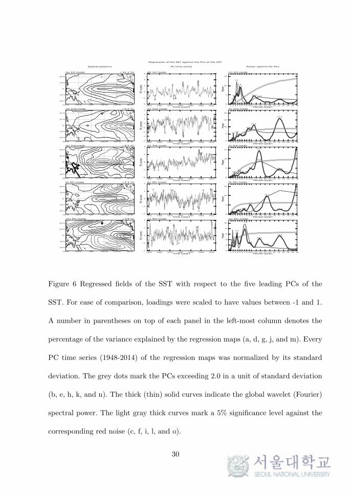
Figure 6 Regressed fields of the SST with respect to the five leading PCs
of the SST. For ease of comparison, loadings were scaled to
have values between -1 and 1. A number in parentheses on top
of each panel in the left-most column denotes the percentage
of the variance explained by the regression maps (a, d, g, j,
and m). Every PC time series (1948-2014) of the regression
maps was normalized by its standard deviation. The grey dots
mark the PCs exceeding 2.0 in a unit of standard deviation
(b, e, h, k, and n). The thick (thin) solid curves indicate the
global wavelet (Fourier) spectral power. The light gray thick
curves mark a 5% significance level against the corresponding
red noise (c, f, i, l, and o). . . . . . . . . . . . . . . . . . . . . 29
Figure 7 As in Fig. 6, but for the regression maps of the MSLP (shaded)
and surface winds (arrows). . . . . . . . . . . . . . . . . . . . 30
Figure 8 As in Fig. 6, but with the RPCs of the SST for the case of 10
loading vectors being rotated. . . . . . . . . . . . . . . . . . . 32
Figure 9 As in Fig. 6, but for the regression maps for the MSLP (shaded)
and surface winds (arrows) with the RPCs of the SST for the
case of 10 loading vectors being rotated. . . . . . . . . . . . . 33
viii

Figure 10 As in Fig. 6, but with the SPCs of the SST by sparse regres-
sion. A triplet of numbers in parentheses on top of each panel
in the left-most column denotes the degree of optimal spar-
sity in the percentage of exact-zero loadings, the percentage
of variances explained by the regressions, and the percentage
of ratio between the variances explained by the sparse regres-
sion and by the linear regression (a, d, g, j, and m). The blue
(red) solid curves indicate the global wavelet (Fourier) spectral
power. The blue (red) dashed curves denote the ratio of the
global wavelet (Fourier) spectral power of the PC time series
of the sparse regression against the SPCs of the SST to that
of the linear regression against the PCs of the SST (c, f, i, l,
and o). . . . . . . . . . . . . . . . . . . . . . . . . . . . . . . . 38
ix

Figure 11 As in Fig. 6, but for the regression maps of the MSLP (shaded)
and surface winds (arrows) with the SPCs of the SST by the
sparse regression. A quadruplet of numbers in parentheses de-
notes the degree of optimal sparsity in the percentage of exact-
zero loadings for the MSLP and surface winds, the percentage
of the variances explained by the regressions, and the per-
centage of ratio between the variances explained by the sparse
regression and by the linear regression (a, d, g, j, and m). The
blue (red) solid curves indicate the global wavelet (Fourier)
spectral power. The blue (red) dashed curves denote the ratio
of the global wavelet (Fourier) spectral power of the PC time
series of the sparse regression against the SPCs of the SST to
that of the linear regression against the PCs of the SST (c, f,
i, l, and o). . . . . . . . . . . . . . . . . . . . . . . . . . . . . . 39
x

Chapter 1
Introduction
The tropical Pacific Ocean has attracted a great deal of attention from climatologists
and environmentalists on account of its large variability in the sea surface temperature
(SST) and its marked impact on global atmospheric circulation. The high degree of
variability shown in Fig. 1 is epitomized by the El Nino Southern Oscillation (ENSO),
which is one of the most important tropical ocean-atmosphere phenomena occurring
in the equatorial Pacific Ocean (Philander, 1990). In relation to the El Nino, we
usually assess the particular spatial patterns of the SST and wind stress anomalies
that persist over the tropical Pacific for several months. Principal component analysis
(PCA), also known as empirical orthogonal function analysis, has played an important
role in identifying the characteristic patterns associated with the ENSO (Legler, 1983;
Diaz and Markgraf, 2000; Ashok et al., 2007). After Larkin and Harrison (2005)
presented the definition of El Nino, Ashok et al. (2007) described ENSO diversity by
introducing the El Nino Modoki (similar but different in Japanese), which is defined
by the second PCA mode of the SST anomaly.
1
Although the ENSO has a huge impact on the Earth, its extent of influence con-
forms to the theoretical framework of equatorial waves. The features are most promi-
nent in the equatorial Pacific basin. Matsuno (1966) showed that equatorial waves
tend to remain close to the equatorial latitudes. In accordance with the argument,
Gill (1980) showed that the atmospheric response to equatorial heating was confined
to equatorial latitudes. More advanced theories on the ENSO such as the delayed
oscillator (Battisti and Hirst, 1989) and recharge-discharge oscillator (Jin, 1997) ad-
dress energy balance and wave motions over the tropical Pacific region straddling the
equator. In considering these facts, we can regard ocean-atmosphere coupled oscilla-
tions in the tropical Pacific such as the ENSO as regionalized spatial patterns with a
particular time period.
PCA has been widely used to capture horizontal patterns in atmospheric motions.
However, the wide use of PCA does not mean it is a perfect solution for separating
and representing a localized feature. Because equatorial waves have a regional scale in
the horizontal domain with a specific periodicity, it may be inappropriate to attempt
to find spatial patterns over an extended latitudinal belt along the equator. A number
of authors have suggested that PCA inherently lacks the ability to represent simple
localized structures in the loading (eigen) vectors (Thurstone, 1931; Kaiser, 1958;
Richman, 1981, 1986; Jolliffe, 1995; Jolliffe et al., 2003; Zou et al., 2006; Hannachi
et al., 2006).
2

As an enhancement of PCA, rotated PCA (RPCA) was proposed by Thurstone
(1931) and has been widely used to facilitate the interpretation of the derived eigen-
modes. The basic concept of RPCA is to rotate a set of loading vectors to maximize
the number of near-zeros in the loading vectors. Lian and Chen (2012) stated that
RPCA could represent the natural variability of SST in the Pacific basin. Recently,
the use of RPCA has been controversial due to its use of several subjective factors
(Jolliffe, 2002; Jolliffe et al., 2003; Hannachi et al., 2006): the selection of loading vec-
tors to be rotated; the choice of rotation criteria (e.g., varimax, quartimax, and the
other 17 measures); and the decision over which object is to be normalized (e.g., load-
ing vectors or PC time series). More importantly, RPCA produces near-zero, rather
than exact-zero, values in the loading vectors (Jolliffe, 2002; Jolliffe et al., 2003).
To overcome the deficiencies of RPCA and PCA, Jolliffe et al. (2003) proposed
sparse principal component analysis (SPCA), referred to as simplified component
technique-LASSO (SCoTLASS). SPCA tends to make eigenvectors much simpler by
increasing the number of exact-zero loadings and simultaneously maximizing the vari-
ances of the corresponding PC time series. The implementation of SPCA is based on
least absolute shrinkage and the selection operator (LASSO) invented by Tibshirani
(1996). Zou et al. (2006) proposed a more elaborate version of SPCA that promoted
the diverse application of SPCA in many fields, e.g., genomics and computer vision.
In such fields, it is as essential to draw out the informative compact features from
3

a given data set as it is in atmospheric science (Lucas et al., 2006; Carvalho et al.,
2008; Wright et al., 2009).
Optimization is not easy in SPCA because it involves a nonconvex problem that
requires more complex computation than a convex problem. Since Zou et al. (2006),
much effort has been devoted to devising an efficient algorithm that requires less
computation (Shen and Huang, 2008; Berthet and Rigollet, 2013). In atmospheric
science, Hannachi et al. (2006) applied the incipient version of SPCA to the MSLP
field of the boreal winter to obtain the SPCA modes and compared them with those
from PCA and RPCA.
This paper is organized as follows. The mathematical basis for each method is
given in section 2. Section 3 summarizes the data used in our analysis. The results
are described in section 4. In section 5, the conclusions are presented and future work
is outlined.
4

90°S
80°S
70°S
60°S
50°S
40°S
30°S
20°S
10°S
0°
10°N
20°N
30°N
40°N
50°N
60°N
70°N
80°N
90°N
0° 30°E 60°E 90°E 120°E 150°E 180° 150°W 120°W 90°W 60°W 30°W
0.2
0.2
0.2
0.2
0.2
0.4
0.4
0.4
0.4
0.4
0.4
0.4
0.4
0.4
0.4
0.4
0.40.40.4
0.4
0.4
0.4
0.40.4
0.4
0.4
0.40.4
0.4 0.4
0.6
0.6
0.6
0.6
0.6
0.6
0.60.6
0.6
0.6 0.6
0.60.6
0.60.
6
0.6
0.8
0.8
0.8
1.0
Figure 1 Distribution of the standard deviation (◦C) of the SST (1948 - 2014).
5

Chapter 2
Methods
2.1 PCA
PCA is a multivariate statistical method to find directions (or eigenmodes) of maximal
variance in a successive manner. For a brief description of PCA, we assume that a
data matrix X comprises n rows (timesteps) and p columns (grid points) with a zero
mean for each column. The covariance matrix may be expressed as
CXX =1
n− 1XTX, (2.1)
whose elements denote the covariances between the time series at any pair of the grid
points. Let v be a column vector indicating a direction such that Xv has maximal
variability. The variance of the time series Xv is
V ar(Xv)
=1
n− 1
(Xv)T (
Xv)
= vTCXXv . (2.2)
A vector v is uniquely determined by solving the constrained maximization prob-
lem as follows.
v = arg maxv
(vTCXXv
)such that vTv = 1 , (2.3)
6

which leads to a simple eigenvalue problem:
CXXv = λv . (2.4)
By using the eigenvector vk (k = 1, 2, · · · , n) in the decreasing order of the eigen-
value λk, the k-th principal component (PC) time series is defined by the projection
of the data matrix X onto the k-th eigenvector vk
zk = Xvk . (2.5)
2.2 RPCA
A rotation matrix R is defined to construct a set of rotated eigenvectors U from a
set of the selected eigenvectors V. The formulation is given as
U = VR , (2.6)
where the rotation matrix R is
R = arg minR
f(VR) . (2.7)
Among the 19 proposed rotation criteria, including orthogonal and oblique rota-
tion (Richman, 1986), the most well-known is the varimax rotation by Kaiser (1958).
This method is employed for comparison with SPCA. It is an orthogonal rotation
criterion expressed as
f(U) =
n∑k=1
[m
m∑i=1
u4ik −( m∑
i=1
u2ik
)2], (2.8)
7

where uik is the i-th element of the rotated k-th eigenvector, defined by uk = vkR,
and m and n are the dimensions of an eigenvector and the number of eigenvectors
to be rotated, respectively. The quantity inside the brackets signifies the variance
of the square of the rotated eigenvector uk (i.e., the spatial variance of the square
of the rotated loadings). The varimax criterion tends to simplify the structure of
eigenvectors resulting from rotation by forcing the loadings to be close to zero or ±1.
2.3 SPCA
SPCA is a constrained PCA with l1-norm regularization and is used to identify the
sparse structure in a given data set. The SPCA is derived by casting PCA into a
multivariate linear regression with a regularization known as LASSO, which makes
loading vectors sparse. The loading vectors of SPCA are determined by minimizing
the cost function defined as
v = arg minv∈Rn
[‖u − Xv‖2F + λLASSO‖v‖1
](2.9a)
= arg minv∈Rn
[‖v − XTu‖2F + λLASSO‖v‖1
](2.9b)
= arg minv∈Rn
[‖X − uvT‖2F + λLASSO‖v‖1
], (2.9c)
where X is the anomaly data matrix of size m× n, u is the PC time series, and v is
the eigenvector (loading vector). Note that ‖ · ‖F and ‖ · ‖1 denote the Frobenius and
8

l1-norms, respectively. They are defined as
‖A‖F =√trace
(ATA
)=
√√√√ m∑i=1
n∑j=1
(aij
)2(2.10a)
‖a‖1 =n∑
i=1
|ai| . (2.10b)
Eq. (9a) expresses the regression of the PC time series u on the anomaly data
matrix X with its coefficients being the eigenvector v. Eq. (9b) corresponds to the
sparse spatial pattern (v) of the anomaly data matrix X that is most correlated with
the PC time series u. Eq. (9c) is used to regress the anomaly data matrix X on the PC
time series u with its coefficient being the eigenvector v. The above three equations
are equivalent to each other with regards to matrix decomposition; however, they
have different uses and benefits in practice. Eq. (9a) and Eq. (9b) were utilized in the
SPCA and sparse regression, respectively.
Without an additional penalty term, the solutions are the same as the eigenvectors
resulting from PCA. In PCA, the minimization of the cost function is straightforward
because of its quadratic relationship to the loading vector v. Difficulty arises when
the cost function contains the l1-norm (LASSO) regularization term because it is
then transmuted into a nonconvex problem. In order to minimize the cost function
with the LASSO regularization, we used the fast iterative soft-thresholding algorithm
(FISTA) by Beck and Teboulle (2009).
Because the PC time series u is dependent on the eigenvector v, we had to proceed
9

with two alternating steps in a recursive manner:
i) To minimize the cost function with respect to the eigenvector v
ii) To compute the PC time series u for the updated eigenvector v
iii) To repeat the above two steps until both u and v converge at a predefined precision
level.
Apparently SPCA is similar to a simple thresholding method in which the load-
ings below a certain threshold value are assigned as zero. However, there exist dis-
tinct differences between the two methods. The simple thresholding method adopts
the hard-thresholding function that has discontinuities at the negative and positive
threshold values, whereas the LASSO penalty term (l1-norm) takes advantage of the
soft-thresholding function that is continuous for the input values (Fig. 2). The hard-
thresholding function impedes the interpretation of obtained eigenvectors and causes
suboptimality in the PC time series due to their dependence on eigenvectors (Cadima
and Jolliffe, 1995).
2.3.1 Estimation of tuning parameters
As the LASSO regularization is controlled by a tuning parameter multiplied by the
l1-norm, the overall performance of SPCA depends on the selection of the LASSO
parameter. The parameter should be optimal with respect to the minimal reconstruc-
tion error or maximal variance explained by each SPCA mode. We will concentrate
on how to determine the optimal values of the LASSO parameter for the SPCA and
10

(a) Soft-thresholding operator
−λ
λ
(b) Hard-thresholding operator
−λ
λ
Figure 2 Soft- and Hard-thresholding functions for the SPCA.
11

the sparse regression.
We consider two types of method for the selection of an optimal parameter: cross-
validation and information criteria. Cross-validation (CV) is used for model selection
and validation by evaluating the predictive performance of a model (Stone, 1974).
The usual procedure is to partition the data into K disjointed subsets and use them
in training and testing a candidate model.
We use the K-fold CV, which is tailored for SPCA. The procedure can be sum-
marized as follows.
Step 1. Split a data matrix X of size m × n into K equal-sized submatrices Xi in a
row-wise manner.
Step 2. For each i ∈{
1, 2, · · · ,K}
, iterate the following procedures.
(a) Let X−i denote the reduced data matrix when Xi is excluded. Find the sparse
loading vector v−i for the matrix X−i. The PC time series ui is obtained by projecting
the submatrix Xi onto v−i as ui = Xiv−i .
(b) Compute the CV root mean squared error (RMSECV ), defined as
RMSECV =
[1
K
K∑i=1
‖Xi − uivT−i‖2F
mn
] 12
. (2.11)
To determine the optimal value of the tuning parameter from the RMSECV , we
apply a ”one-standard error” rule in which the most parsimonious model whose error
falls within one standard deviation above the error of the best model is regarded as
the best model (Hastie et al., 2009).
12
In the literature relating to model selection, CV is known to be loss efficient but
selection inconsistent, especially, for regularized problems (Wang et al., 2009; Zhang
et al., 2010; Chand, 2012). That is, the shrinkage (LASSO) parameter chosen by CV
may not identify the true model, as was formally verified by Wang et al. (2007).
Recent studies show that the Bayesian information criterion (BIC) and its variants
are able to identify the true model among a number of candidates (Wang et al., 2007;
Wang and Leng, 2007; Chand, 2012).
The BIC is a suitable measure of the trade-off between the goodness-of-fit and
the complexity of a model. It is defined as
BIC = − 2logL(θ)
+ k log(N)
, (2.12)
where L(θ)
denotes the likelihood function of the parameters θ in a model, k is the
degrees of freedom of a model, and N is the number of samples. The model with the
smallest BIC is preferred and is selected as the best. Because we are dealing with the
matrix (Frobenius) norm (‖·‖F ), we adopt a form of generalized information criterion
(GIC) suited for its use in the matrix as in Sill et al. (2015):
GICmatrix = (mn)log
(‖X − uvT‖2F
mn
)+ knonzero
(log m
)(log n
). (2.13)
Furthermore, we propose a new criterion to objectively select the sparse patterns
of the real variability of climate systems such as the ENSO. The criterion is ”rate
of information loss (ROIL),” which is the ratio of percent decrease in the explained
13

variance (δVAR) to that of the degrees of freedom (δDF ) of the model. Its functional
form is
ROIL = − δVAR
δDF. (2.14)
Eq. 14 indicates how fast the explained variance (information) decreases against the
growing parsimony (diminishing DF) of the model. Consequently, we can define an
optimal sparsity where the ROIL reaches unity.
We calculated and presented all three criteria to allow for the selection of the best
sparse patterns embedded in the variation of SST, MSLP, and surface winds over the
tropical Pacific.
14

Chapter 3
Data
The data used for the analysis are the monthly mean values of SST, MSLP, and surface
winds. The SST data were obtained from the Centennial in situ Observation-Based
Estimate (COBE). The MSLP and surface wind data were obtained from the National
Center for Environmental Prediction (NCEP)/National Center for Atmospheric Re-
search (NCAR) Reanalysis. These data were provided by the National Oceanic and
Atmospheric Administration (NOAA)/Earth System Research Laboratory (ESRL)
via their website at http://www.esrl.noaa.gov/psd/.
The COBE dataset is a spatially complete, interpolated 1◦×1◦ SST product from
1891 to the present. It combines SSTs from various sources such as the International
Comprehensive Ocean-Atmosphere Data Set, Japanese Kobe collection, and ships
and buoys (Ishii et al., 2005). The NCEP/NCAR Reanalysis dataset was produced
using a state-of-the-art analysis/forecast system by performing data assimilation of
past data from 1948 to present. The dataset covers the globe with a resolution of
2.5◦ × 2.5◦ (Kalnay et al., 1996).
15

The SST data were regridded onto a 2.5◦ × 2.5◦ grid to be consistent with the
resolution of the MSLP and surface wind data. For consistency with that of the
NCEP/NCAR data, we adjusted the analyzed time period from January 1948 to
December 2014.
The analysis domain was bounded by 25◦S − 25◦N, 120◦E − 80◦W , which covers
the tropical Pacific Ocean.
As a preprocess, we removed annual variation by subtracting the calendar mean
value for each month at each grid point of the analysis domain. Then, the anomalies
were multiplied by the square root of the latitudinal cosine factor to account for
the decreasing grid interval in the meridional direction. Because the anomaly fields
were analyzed, the SST, MSLP, and surface winds refer to their respective anomalies,
unless specified otherwise.
16

Chapter 4
Results
We present results for the PCA, RPCA, and SPCA of the SST data. We also show
the linear and sparse regression of the MSLP and surface winds. In the regression
analysis, we used the PC time series of the PCA, RPCA, and SPCA modes of the
SST data; the three time series are named PCs, RPCs, and SPCs, respectively. For
the surface winds, we employed a complex number representation for the vector wind,
as in Hardy (1977).
4.1 SST
4.1.1 PCA modes
Figure 3 shows the five leading PCA modes and the power spectra of the correspond-
ing PCs of SST over the tropical Pacific.
The first mode (Fig. 3(a)) expresses the canonical El Nino pattern, which has
a tongue-shaped protrusion of the positive anomaly. The power spectra of the cor-
responding PC (Fig. 3(c)) has two pronounced peaks at periods of 3.5-years and
17

5-years, which were described as ENSO signals by Rasmusson and Carpenter (1982)
and White and Tourre (2003).
The second mode (Fig. 3(d)) displays a bimodal pattern that has a wedge-shaped
negative anomaly abutting the west coast of South America and a notch-shaped
positive anomaly encircling the former. This mode bears a partial resemblance to El
Nino Modoki (Ashok et al., 2007), except for the fact that the mode does not indicate
an anomalous variation in SST in the far western Pacific with the same sign as in
the eastern equatorial Pacific. The power spectra of the second mode (Fig. 3(f)) show
two distinct peaks at 11-year and 22.5-year periods.
The third mode (Fig. 3(g)) exhibits the central-Pacific (CP)-type of ENSO (Kao
and Yu, 2008) or the mixed type of ENSO (Kug et al., 2009) pattern that resides in
the Nino-3.4 region (5◦S−5◦N, 170◦W −120◦W ), as well as the SST variation of the
western Pacific warm pool (WPWP). Yan et al. (1992); Ho et al. (1995) defined the
WPWP as an area in which SST is higher than 28◦C in the western tropical Pacific.
It is noticeable that the spectral power of the third mode (Fig. 3(i)) peaks at the
13.4-year period.
The fourth and fifth modes (Fig. 3(j) and Fig. 3(m)) display the North Pacific
meridional mode (NPMM), demonstrated by Chiang and Vimont (2004), and the
South Pacific meridional mode (SPMM), proposed by Zhang et al. (2014), which are in
phase and have centers of action located off the equator by 15−20◦. Both the NPMM
18

and the SPMM represent mid-latitude atmospheric variability and subtropical air-sea
thermodynamic coupling (Chiang and Vimont, 2004; Zhang et al., 2014). There exist
several significant peaks over short to long periods in the power spectra of the PCs
(Fig. 3(l) and Fig. 3(o)), which are characteristic of the two Pacific meridional modes
(Zhang et al., 2014).
4.1.2 RPCA modes
All the PCA modes are full of nonzero values and such a complicated pattern hinders
the relevant and succinct interpretation of the underlying physical mechanisms. As
an intermediate stage, we conducted RPCA of the SST data with a different number
(10, 20, and 30) of loading vectors being rotated. (Table 1) We assessed the properties
of the RPCA modes and compared them with the SPCA modes; this will be discussed
later. We applied rotation to the K leading PCA eigenvectors with the varimax
criterion.
The five leading RPCA modes of the SST data are shown for the case of K = 10 in
Fig. 4. One of the most striking features is that the horizontal patterns tend to become
a circular-shaped monopole structure as the number K increases. The cores with the
highest or lowest loading are highly concentrated within an area of about 20◦ latitude
by 45◦ longitude, which shows morphological resemblance to a one-point correlation
map. However, there remain a great number of nonzero loadings throughout the
entire analysis domain, obstructing any effective interpretation (Fig. 4(a), Fig. 4(d),
19

PCA modes of the SST
Spatial patterns PC time series Power spectra for PCs
(a) 1st mode ( 41.1 %) (b) 1st mode (c) 1st mode
20°S
10°S
0°
10°N
20°N
120°E 150°E 180° 150°W 120°W 90°W 1950 1960 1970 1980 1990 2000 2010Time (year)
4
2
0
2
4
6
PC sc
ores
1 2 3 4 5 6 7 8 910 12 14 16 18 20 22 24 26 28 30Period (year)
0
5
10
15
Powe
r
3.7
5.3
11.2
16.9
22.4
13.4
4.8
3.5
2.5
2.2
(d) 2nd mode ( 9.2 %) (e) 2nd mode (f) 2nd mode
20°S
10°S
0°
10°N
20°N
120°E 150°E 180° 150°W 120°W 90°W 1950 1960 1970 1980 1990 2000 2010Time (year)
4
3
2
1
0
1
2
3
PC sc
ores
1 2 3 4 5 6 7 8 910 12 14 16 18 20 22 24 26 28 30Period (year)
0
5
10
15
20
Powe
r
2.1
3.75.1
8.5
11.0
22.4
9.6
5.2
3.72.1
(g) 3rd mode ( 8.5 %) (h) 3rd mode (i) 3rd mode
20°S
10°S
0°
10°N
20°N
120°E 150°E 180° 150°W 120°W 90°W 1950 1960 1970 1980 1990 2000 2010Time (year)
4
2
0
2
4
PC sc
ores
1 2 3 4 5 6 7 8 910 12 14 16 18 20 22 24 26 28 30Period (year)
0
5
10
15
Powe
r
2.53.4
6.0
9.7
13.4
22.4
13.4
4.8
3.72.4
2.1
(j) 4th mode ( 4.3 %) (k) 4th mode (l) 4th mode
20°S
10°S
0°
10°N
20°N
120°E 150°E 180° 150°W 120°W 90°W 1950 1960 1970 1980 1990 2000 2010Time (year)
4
2
0
2
4
PC sc
ores
1 2 3 4 5 6 7 8 910 12 14 16 18 20 22 24 26 28 30Period (year)
0
5
10
15
Powe
r
2.64.0
6.8
9.5
16.7
22.46.74.8
3.02.4
(m) 5th mode ( 3.8 %) (n) 5th mode (o) 5th mode
20°S
10°S
0°
10°N
20°N
120°E 150°E 180° 150°W 120°W 90°W 1950 1960 1970 1980 1990 2000 2010Time (year)
4
2
0
2
4
PC sc
ores
1 2 3 4 5 6 7 8 910 12 14 16 18 20 22 24 26 28 30Period (year)
0
2
4
6
8
10Po
wer 3.6
7.1
9.5
13.5
16.4
22.4
7.4
3.7
2.4
Figure 3 Five leading PCA modes of the SST over the tropical Pacific. For ease
of comparison, loadings were scaled to have values between -1 and 1. A number in
parentheses on top of each panel in the left-most column denotes the percentage of
the variance explained by the corresponding PCA modes (a, d, g, j, and m). Every
PC time series (1948-2014) was normalized by its standard deviation. The gray dots
mark the PCs exceeding 2.0 in a unit of standard deviation (b, e, h, k, and n). The
thick (thin) solid curves indicate the global wavelet (Fourier) spectral power. The
light gray thick curves mark a 5% significance level against the corresponding red
noise (c, f, i, l, and o).
20

Fig. 4(g), Fig. 4(j), and Fig. 4(m)).
Another feature of RPCA is the differential reduction of the variance explained
by each RPCA mode. The explained variances are redistributed among the new load-
ing vectors resulting from the rotation, which ultimately spreads the variance evenly
among the eigenmodes. The consequence of this may be critical in ranking the eigen-
modes in descending order of their explained variance when two or more eigenvectors
are degenerate, so that the corresponding spatial patterns are indistinguishable from
each other. The issue can be corroborated by the similitude in the power spectra of
the RPCs of the SST data (Fig. 4) and in the regression fields of the SST data against
the RPCs of the SST data (Fig. 7). The regression analysis is discussed in detail later.
The power spectra of the four leading RPCs have their highest peaks at periods
ranging from 3 to 5 years, which betokens the archetypal ENSO mode. However,
it is difficult to say any distinctive features with respect to and temporal variation
in the power spectra of the RPCs; drawing an acceptable conclusion requires further
investigation of the effect. In our analysis, RPCA tends to localize the spatial patterns
without splitting up the signatures of the temporal variations for each RPCA mode
(Fig. 4(c), Fig. 4(f), Fig. 4(i), Fig. 4(l))
4.1.3 SPCA modes
Figure 5 shows the five leading SPCA modes that are considered to be optimal with
regard to the averaged sparsity of the three criteria given in Table 2. As expected,
21
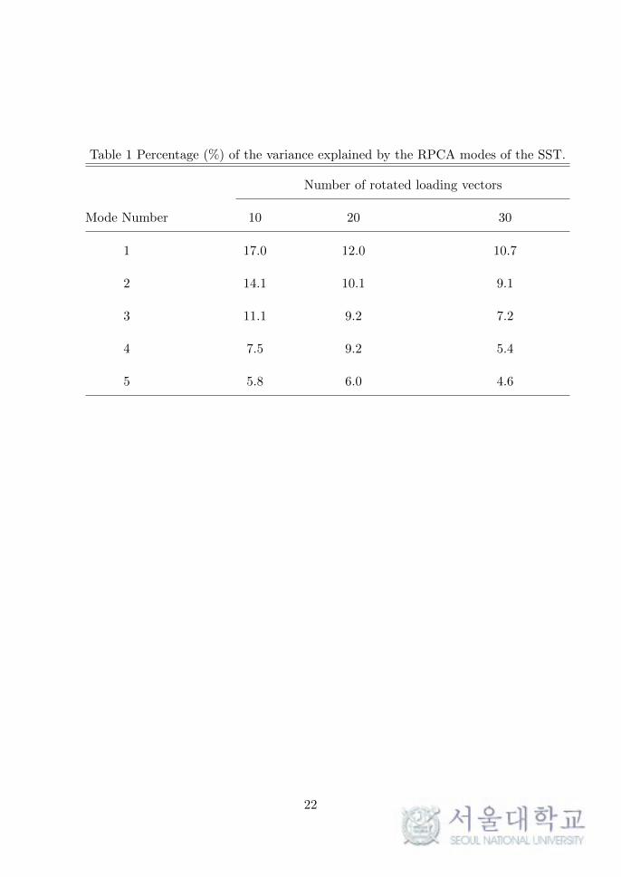
Table 1 Percentage (%) of the variance explained by the RPCA modes of the SST.
Number of rotated loading vectors
Mode Number 10 20 30
1 17.0 12.0 10.7
2 14.1 10.1 9.1
3 11.1 9.2 7.2
4 7.5 9.2 5.4
5 5.8 6.0 4.6
22

RPCA modes of the SST(Number of loading vectors being rotated : 10)
Spatial patterns PC time series Power spectra
(a) 1st mode ( 17.0 %) (b) 1st mode (c) 1st mode
20°S
10°S
0°
10°N
20°N
120°E 150°E 180° 150°W 120°W 90°W 1950 1960 1970 1980 1990 2000 2010Time (year)
6
4
2
0
2
4
PC sc
ores
1 2 3 4 5 6 7 8 910 12 14 16 18 20 22 24 26 28 30Period (year)
0
5
10
15
Powe
r
3.6
5.3
11.213.3
22.4
13.4
4.8
3.5
2.5
2.2
(d) 2nd mode ( 14.1 %) (e) 2nd mode (f) 2nd mode
20°S
10°S
0°
10°N
20°N
120°E 150°E 180° 150°W 120°W 90°W 1950 1960 1970 1980 1990 2000 2010Time (year)
6
4
2
0
2
4
PC sc
ores
1 2 3 4 5 6 7 8 910 12 14 16 18 20 22 24 26 28 30Period (year)
0
5
10
15
Powe
r
2.1
3.6
5.3
6.7 13.5
16.6
22.4
13.4
5.2
3.5
2.2
(g) 3rd mode ( 11.1 %) (h) 3rd mode (i) 3rd mode
20°S
10°S
0°
10°N
20°N
120°E 150°E 180° 150°W 120°W 90°W 1950 1960 1970 1980 1990 2000 2010Time (year)
4
2
0
2
4
PC sc
ores
1 2 3 4 5 6 7 8 910 12 14 16 18 20 22 24 26 28 30Period (year)
0
5
10
15
Powe
r
3.8
5.0
11.3
22.4
13.44.8
3.5
2.5
(j) 4th mode ( 7.5 %) (k) 4th mode (l) 4th mode
20°S
10°S
0°
10°N
20°N
120°E 150°E 180° 150°W 120°W 90°W 1950 1960 1970 1980 1990 2000 2010Time (year)
4
2
0
2
4
PC sc
ores
1 2 3 4 5 6 7 8 910 12 14 16 18 20 22 24 26 28 30Period (year)
0
2
4
6
8
10
Powe
r
3.7
5.3
11.2
17.1
22.4
4.8
3.5
2.52.1
(m) 5th mode ( 5.8 %) (n) 5th mode (o) 5th mode
20°S
10°S
0°
10°N
20°N
120°E 150°E 180° 150°W 120°W 90°W 1950 1960 1970 1980 1990 2000 2010Time (year)
4
2
0
2
4
PC sc
ores
1 2 3 4 5 6 7 8 910 12 14 16 18 20 22 24 26 28 30Period (year)
0
5
10
15
Powe
r
4.3
10.0
16.9
22.4
4.8
Figure 4 As in figure 3, but for the RPCA modes of the SST with 10 loading vectors
being rotated.
23
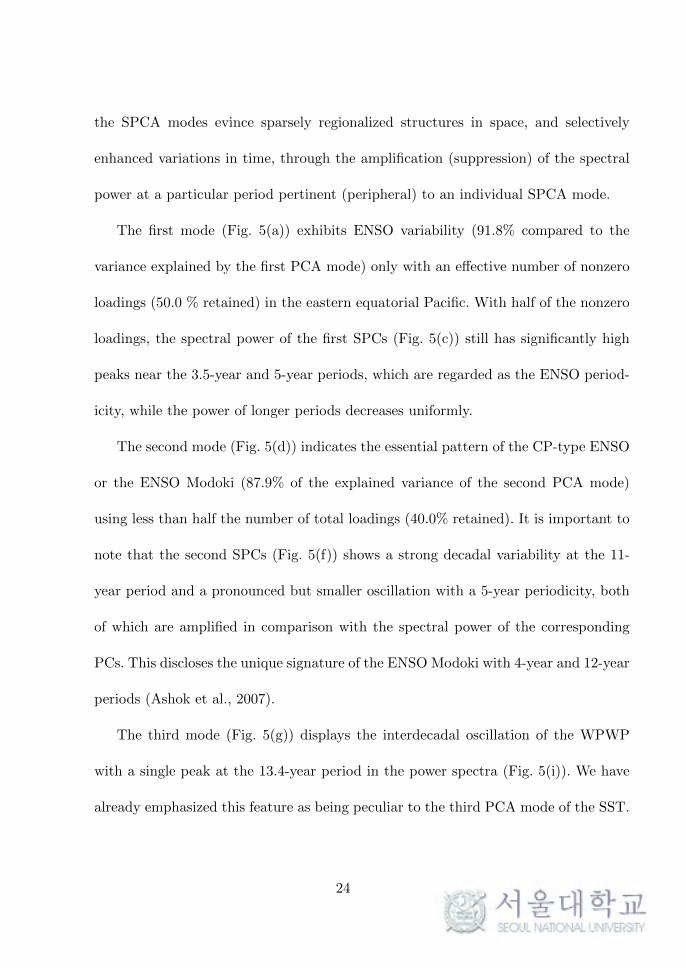
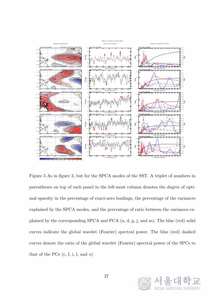
the SPCA modes evince sparsely regionalized structures in space, and selectively
enhanced variations in time, through the amplification (suppression) of the spectral
power at a particular period pertinent (peripheral) to an individual SPCA mode.
The first mode (Fig. 5(a)) exhibits ENSO variability (91.8% compared to the
variance explained by the first PCA mode) only with an effective number of nonzero
loadings (50.0 % retained) in the eastern equatorial Pacific. With half of the nonzero
loadings, the spectral power of the first SPCs (Fig. 5(c)) still has significantly high
peaks near the 3.5-year and 5-year periods, which are regarded as the ENSO period-
icity, while the power of longer periods decreases uniformly.
The second mode (Fig. 5(d)) indicates the essential pattern of the CP-type ENSO
or the ENSO Modoki (87.9% of the explained variance of the second PCA mode)
using less than half the number of total loadings (40.0% retained). It is important to
note that the second SPCs (Fig. 5(f)) shows a strong decadal variability at the 11-
year period and a pronounced but smaller oscillation with a 5-year periodicity, both
of which are amplified in comparison with the spectral power of the corresponding
PCs. This discloses the unique signature of the ENSO Modoki with 4-year and 12-year
periods (Ashok et al., 2007).
The third mode (Fig. 5(g)) displays the interdecadal oscillation of the WPWP
with a single peak at the 13.4-year period in the power spectra (Fig. 5(i)). We have
already emphasized this feature as being peculiar to the third PCA mode of the SST.
24
With the substantial removal of insignificant loadings (40.0% retained), the SPCA
mode maintains 78.0% of the explained variance of the corresponding PCA mode.
This decadal variability may have a connection with the warm pool (WP) El Nino
suggested by Kug et al. (2009), which varies with 10 to 15-year periods in the central
Pacific. Our analysis suggests that this mode is likely to bear a relationship with the
WP El Nino.
The fourth mode (Fig. 5(j)) reveals the SPMM solely, with all other signals ef-
fectively eliminated. While 30% of nonzero loadings are retained, the total variance
responsible for the SPMM remains almost the same as the PCA mode (99.3% of the
variance explained by the fourth PCA mode). Furthermore, this SPCA mode shows
a power spectra (Fig. 5(l)) that has many local peaks over a broad range of periods
(3.8-, 6.6-, 16.7-, 22.4-years in the global wavelet power spectra), which better indi-
cates the traits of temporal variations in the SPMM than did the corresponding PCA
mode.
The fifth SPCA mode (Fig. 5(m)) depicts the NPMM, in which the two oppo-
site anomalous SST patterns appear in the northeastern subtropical Pacific and the
central tropical Pacific. While a trace of the ENSO-like pattern is shown in the south-
eastern Pacific, its spectral power (Fig. 5(o)) became very weak compared to the fifth
PCA mode by amplifying that of the decadal and interdecadal periodicities peaking
at 8.3- and 13.4-year periods.
25
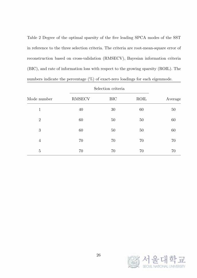
Table 2 Degree of the optimal sparsity of the five leading SPCA modes of the SST
in reference to the three selection criteria. The criteria are root-mean-square error of
reconstruction based on cross-validation (RMSECV), Bayesian information criteria
(BIC), and rate of information loss with respect to the growing sparsity (ROIL). The
numbers indicate the percentage (%) of exact-zero loadings for each eigenmode.
Selection criteria
Mode number RMSECV BIC ROIL Average
1 40 30 60 50
2 60 50 50 60
3 60 50 50 60
4 70 70 70 70
5 70 70 70 70
26
SPCA modes of the SST
Spatial patterns PC time series Power spectra of PCs
(a) 1st mode (50.0%, 37.7%, 91.8%) (b) 1st mode (c) 1st mode
20°S
10°S
0°
10°N
20°N
120°E 150°E 180° 150°W 120°W 90°W 1950 1960 1970 1980 1990 2000 2010Time (year)
4
2
0
2
4
6
PC sc
ores
1 2 3 4 5 6 7 8 910 12 14 16 18 20 22 24 26 28 30Period (year)
0
5
10
15
Powe
r
3.6
5.3
11.2
16.922.4
13.4
4.8
3.5
2.5
2.2
0.5
1.0
1.5
2.0
2.5
3.0
3.5
4.0
4.5
5.0
Ratio
(d) 2nd mode (60.0%, 8.0%, 87.9%) (e) 2nd mode (f) 2nd mode
20°S
10°S
0°
10°N
20°N
120°E 150°E 180° 150°W 120°W 90°W 1950 1960 1970 1980 1990 2000 2010Time (year)
4
3
2
1
0
1
2
3
PC sc
ores
1 2 3 4 5 6 7 8 910 12 14 16 18 20 22 24 26 28 30Period (year)
0
5
10
15
Powe
r
2.3
4.9
11.1
22.4
11.2
4.5
2.0
0.5
1.0
1.5
2.0
2.5
3.0
3.5
4.0
4.5
5.0
Ratio
(g) 3rd mode (60.0%, 6.6%, 78.0%) (h) 3rd mode (i) 3rd mode
20°S
10°S
0°
10°N
20°N
120°E 150°E 180° 150°W 120°W 90°W 1950 1960 1970 1980 1990 2000 2010Time (year)
4
2
0
2
4
PC sc
ores
1 2 3 4 5 6 7 8 910 12 14 16 18 20 22 24 26 28 30Period (year)
0
5
10
15
Powe
r
2.53.4
5.79.1
13.4
22.4
13.4
5.23.52.5
2.1
0.5
1.0
1.5
2.0
2.5
3.0
3.5
4.0
4.5
5.0
Ratio
(j) 4th mode (70.0%, 4.3%, 99.3%) (k) 4th mode (l) 4th mode
20°S
10°S
0°
10°N
20°N
120°E 150°E 180° 150°W 120°W 90°W 1950 1960 1970 1980 1990 2000 2010Time (year)
4
2
0
2
4
PC sc
ores
1 2 3 4 5 6 7 8 910 12 14 16 18 20 22 24 26 28 30Period (year)
0
5
10
15
Powe
r
2.7
3.8
5.0
6.6
9.7
16.7
22.4
4.83.7
2.4 0.5
1.0
1.5
2.0
2.5
3.0
3.5
4.0
4.5
5.0
Ratio
(m) 5th mode (70.0%, 3.1%, 82.5%) (n) 5th mode (o) 5th mode
20°S
10°S
0°
10°N
20°N
120°E 150°E 180° 150°W 120°W 90°W 1950 1960 1970 1980 1990 2000 2010Time (year)
6
4
2
0
2
4
PC sc
ores
1 2 3 4 5 6 7 8 910 12 14 16 18 20 22 24 26 28 30Period (year)
0
2
4
6
8
10
Powe
r
3.6
8.3
13.4
22.4
7.4
3.5
2.4
0.5
1.0
1.5
2.0
2.5
3.0
3.5
4.0
4.5
5.0
Ratio
1.0 0.8 0.6 0.4 0.2 0.0 0.2 0.4 0.6 0.8 1.0
Figure 5 As in figure 3, but for the SPCA modes of the SST. A triplet of numbers in
parentheses on top of each panel in the left-most column denotes the degree of opti-
mal sparsity in the percentage of exact-zero loadings, the percentage of the variances
explained by the SPCA modes, and the percentage of ratio between the variances ex-
plained by the corresponding SPCA and PCA (a, d, g, j, and m). The blue (red) solid
curves indicate the global wavelet (Fourier) spectral power. The blue (red) dashed
curves denote the ratio of the global wavelet (Fourier) spectral power of the SPCs to
that of the PCs (c, f, i, l, and o)
27
4.2 Regressed MSLP and surface winds
The spatial structures of the atmospheric motions may have a close relationship with
those of the SST over the Pacific Ocean. In order to delineate the horizontal patterns
of the atmospheric variations, we regressed the MSLP and surface winds against, as
reference time series, the PCs, RPCs, and SPCs of the SST.
4.2.1 Regression against PCs
Figure 9 shows the regression map of the MSLP and surface winds, each of which was
regressed on the five leading PCs of the SST.
The regression for the first mode (Fig. 9(a)) displays a dipole structure straddling
the dateline between the Eastern and the Western Hemisphere in both the MSLP
and the surface winds. It reveals the typical shape of the Southern Oscillation (SO).
The second mode-based regression of the MSLP (Fig. 9(d)) shows that of the
El Nino Modoki. The regression map is characterized by a negative anomaly in the
MSLP over the central Pacific and enhanced westerly anomalies over the western
tropical Pacific.
The third regression (Fig. 9(g)) exhibits the atmospheric responses to both a
positive anomaly of the SST at the WPWP and a small area of strongly negative
SST anomaly in the central equatorial Pacific. The easterly (westerly) anomalies are
dominant west (east) of 150◦W .
28

The fourth and fifth regression (Fig. 9(j) and Fig. 9(m)) display the characteristics
of the NPMM and the SPMM, which are marked by the anomalous MSLP centers in
the subtropics of the Northern Hemisphere (NH) and the Southern Hemisphere (SH)
along with the cross-equatorial surface wind anomalies.
4.2.2 Regression against RPCs
Figure 10 shows the regression of the MSLP and the surface winds against the RPCs
of the SST. We can see a well-organized pattern in both the MSLP and the surface
winds for all the modes (Fig. 9(a), Fig. 9(d), Fig. 9(g), Fig. 9(j), and Fig. 9(m)); in
essence, this is indicative of the ENSO mode.
To elucidate the source of the similitude among the regression maps, we regressed
the SST against the PCs, RPCs, and SPCs of the SST to enable reconstruction of
the five leading modes of the SST itself. The regression based on the PCs (Fig. 6(a),
Fig. 6(d), Fig. 6(g), Fig. 6(j), and Fig. 6(m)) and SPCs (Fig. 10(a), Fig. 10(d), Fig.
10(g), Fig. 10(j), and Fig. 10(m)) correctly reproduced the original PCA and SPCA
modes in relation to both the spatial pattern and temporal variation. In contrast,
the regression based on the RPCs (Fig. 8(a), Fig. 8(d), Fig. 8(g), Fig. 8(j), and Fig.
8(m)) failed to replicate each of the original RPCA modes and only generated the
ENSO-related mode. This problem, as aforementioned, is ascribed to the rotation
of loading vectors for the purpose of obtaining the sparse and localized eigenmodes
without considering any other factors. RPCA seems incapable of discriminating the
29
Regression of the SST against the PCs of the SST
Spatial patterns PC time series Power spectra for PCs
(a) 1st mode ( 41.1 %) (b) 1st mode (c) 1st mode
20°S
10°S
0°
10°N
20°N
120°E 150°E 180° 150°W 120°W 90°W 1950 1960 1970 1980 1990 2000 2010Time (year)
4
2
0
2
4
6
PC sc
ores
1 2 3 4 5 6 7 8 910 12 14 16 18 20 22 24 26 28 30Period (year)
0
5
10
15
Powe
r
3.7
5.3
11.2
16.9
22.4
13.4
4.8
3.5
2.5
2.2
(d) 2nd mode ( 9.2 %) (e) 2nd mode (f) 2nd mode
20°S
10°S
0°
10°N
20°N
120°E 150°E 180° 150°W 120°W 90°W 1950 1960 1970 1980 1990 2000 2010Time (year)
4
3
2
1
0
1
2
3
PC sc
ores
1 2 3 4 5 6 7 8 910 12 14 16 18 20 22 24 26 28 30Period (year)
0
5
10
15
20
Powe
r
2.1
3.75.1
8.5
11.0
22.4
9.6
5.2
3.72.1
(g) 3rd mode ( 8.5 %) (h) 3rd mode (i) 3rd mode
20°S
10°S
0°
10°N
20°N
120°E 150°E 180° 150°W 120°W 90°W 1950 1960 1970 1980 1990 2000 2010Time (year)
4
2
0
2
4
PC sc
ores
1 2 3 4 5 6 7 8 910 12 14 16 18 20 22 24 26 28 30Period (year)
0
5
10
15
Powe
r
2.53.4
6.0
9.7
13.4
22.4
13.4
4.8
3.72.4
2.1
(j) 4th mode ( 4.3 %) (k) 4th mode (l) 4th mode
20°S
10°S
0°
10°N
20°N
120°E 150°E 180° 150°W 120°W 90°W 1950 1960 1970 1980 1990 2000 2010Time (year)
4
2
0
2
4
PC sc
ores
1 2 3 4 5 6 7 8 910 12 14 16 18 20 22 24 26 28 30Period (year)
0
5
10
15
Powe
r
2.64.0
6.8
9.5
16.7
22.46.74.8
3.02.4
(m) 5th mode ( 3.8 %) (n) 5th mode (o) 5th mode
20°S
10°S
0°
10°N
20°N
120°E 150°E 180° 150°W 120°W 90°W 1950 1960 1970 1980 1990 2000 2010Time (year)
4
2
0
2
4
PC sc
ores
1 2 3 4 5 6 7 8 910 12 14 16 18 20 22 24 26 28 30Period (year)
0
2
4
6
8
10Po
wer 3.6
7.1
9.5
13.5
16.4
22.4
7.4
3.7
2.4
Figure 6 Regressed fields of the SST with respect to the five leading PCs of the
SST. For ease of comparison, loadings were scaled to have values between -1 and 1.
A number in parentheses on top of each panel in the left-most column denotes the
percentage of the variance explained by the regression maps (a, d, g, j, and m). Every
PC time series (1948-2014) of the regression maps was normalized by its standard
deviation. The grey dots mark the PCs exceeding 2.0 in a unit of standard deviation
(b, e, h, k, and n). The thick (thin) solid curves indicate the global wavelet (Fourier)
spectral power. The light gray thick curves mark a 5% significance level against the
corresponding red noise (c, f, i, l, and o).
30

Regression of the MSLP and surface winds against the PCs of the SST
Spatial patterns PC time series Power spectra for PCs
(a) 1st mode ( 23.0 %) (b) 1st mode (c) 1st mode
20°S
10°S
0°
10°N
20°N
120°E 150°E 180° 150°W 120°W 90°W 1950 1960 1970 1980 1990 2000 2010Time (year)
4
2
0
2
4
6
PC sc
ores
1 2 3 4 5 6 7 8 910 12 14 16 18 20 22 24 26 28 30Period (year)
0
5
10
15
Powe
r
3.6
5.311.1
16.6
22.4
13.4
4.8
3.5
2.5
2.1
(d) 2nd mode ( 7.4 %) (e) 2nd mode (f) 2nd mode
20°S
10°S
0°
10°N
20°N
120°E 150°E 180° 150°W 120°W 90°W 1950 1960 1970 1980 1990 2000 2010Time (year)
6
4
2
0
2
4
PC sc
ores
1 2 3 4 5 6 7 8 910 12 14 16 18 20 22 24 26 28 30Period (year)
0
2
4
6
8
10
Powe
r
2.0
3.64.75.6
10.8
16.9
22.4
11.2
4.8
3.7
2.5
2.0
(g) 3rd mode ( 22.6 %) (h) 3rd mode (i) 3rd mode
20°S
10°S
0°
10°N
20°N
120°E 150°E 180° 150°W 120°W 90°W 1950 1960 1970 1980 1990 2000 2010Time (year)
6
4
2
0
2
4
PC sc
ores
1 2 3 4 5 6 7 8 910 12 14 16 18 20 22 24 26 28 30Period (year)
0
5
10
15
Powe
r
2.63.6
5.17.1
11.2
22.4
11.2
4.8
3.5
2.5
2.1
(j) 4th mode ( 7.0 %) (k) 4th mode (l) 4th mode
20°S
10°S
0°
10°N
20°N
120°E 150°E 180° 150°W 120°W 90°W 1950 1960 1970 1980 1990 2000 2010Time (year)
4
2
0
2
4
PC sc
ores
1 2 3 4 5 6 7 8 910 12 14 16 18 20 22 24 26 28 30Period (year)
0
2
4
6
8
10
Powe
r
3.6
5.2
11.4
16.7
22.44.8
3.5
2.5
2.2
(m) 5th mode ( 12.5 %) (n) 5th mode (o) 5th mode
20°S
10°S
0°
10°N
20°N
120°E 150°E 180° 150°W 120°W 90°W 1950 1960 1970 1980 1990 2000 2010Time (year)
6
4
2
0
2
4
6
PC sc
ores
Unit vector1 2 3 4 5 6 7 8 910 12 14 16 18 20 22 24 26 28 30
Period (year)
0
5
10
15
Powe
r
2.0
3.65.4
10.113.3
22.4
4.8
3.5
2.52.1
Figure 7 As in Fig. 6, but for the regression maps of the MSLP (shaded) and surface
winds (arrows).
31

distinct modes, each of which should possess a characteristic spatiotemporal signature;
therefore, the regression maps end up being very similar to each other in terms of
their overall structures.
4.2.3 Regression against the SPCs
To identify coupled patterns in the ocean-atmosphere system, we applied linear re-
gression to the MSLP and surface wind anomalies associated with the SPCA modes
of the SST. It was found that the patterns of the atmospheric fields were similar to
those regressed with the PCs. This is due to the fact that the sparse structures of the
SPCs cannot automatically be transferred to the regression map without an additional
procedure to make them sparse. To obtain the sparse structures of the atmospheric
variables, we applied the sparse regression, which is mathematically equivalent to
the SPCA in the sense that the SPCA is based on the recursive utilization of linear
regression with the LASSO regularization.
With the averaged sparsity of the three selection criteria given in Table 3 in terms
of MSLP and surface winds, the optimal sparse patterns were found by sparsely re-
gressing each variable with the SPCs of the SST. Figure 11 shows the sparse regression
maps of the MSLP and surface winds that are marked by regionalized centers of vari-
ation for each variable. Given the fact that the regressed fields of the MSLP and
surface winds were analyzed separately by sparse regression, it is noteworthy that
they have substantial consistency with each other.
32

Regression of the SST against the RPCs of the SST(Number of loading vectors being rotated : 10)
Spatial patterns PC time series Power spectra of PCs
(a) 1st mode ( 40.5 %) (b) 1st mode (c) 1st mode
20°S
10°S
0°
10°N
20°N
120°E 150°E 180° 150°W 120°W 90°W 1950 1960 1970 1980 1990 2000 2010Time (year)
6
4
2
0
2
4
PC sc
ores
1 2 3 4 5 6 7 8 910 12 14 16 18 20 22 24 26 28 30Period (year)
0
5
10
15
Powe
r
3.6
5.3
11.2
16.722.4
13.4
4.8
3.5
2.5
2.2
(d) 2nd mode ( 38.3 %) (e) 2nd mode (f) 2nd mode
20°S
10°S
0°
10°N
20°N
120°E 150°E 180° 150°W 120°W 90°W 1950 1960 1970 1980 1990 2000 2010Time (year)
6
4
2
0
2
4
PC sc
ores
1 2 3 4 5 6 7 8 910 12 14 16 18 20 22 24 26 28 30Period (year)
0
5
10
15
Powe
r
3.6
5.3
11.2
16.922.4
13.4
4.8
3.5
2.6
2.2
(g) 3rd mode ( 37.5 %) (h) 3rd mode (i) 3rd mode
20°S
10°S
0°
10°N
20°N
120°E 150°E 180° 150°W 120°W 90°W 1950 1960 1970 1980 1990 2000 2010Time (year)
4
2
0
2
4
PC sc
ores
1 2 3 4 5 6 7 8 910 12 14 16 18 20 22 24 26 28 30Period (year)
0
5
10
15
Powe
r3.7
5.2
11.2
22.4
13.4
4.8
3.5
2.5
(j) 4th mode ( 37.3 %) (k) 4th mode (l) 4th mode
20°S
10°S
0°
10°N
20°N
120°E 150°E 180° 150°W 120°W 90°W 1950 1960 1970 1980 1990 2000 2010Time (year)
4
2
0
2
4
6
PC sc
ores
1 2 3 4 5 6 7 8 910 12 14 16 18 20 22 24 26 28 30Period (year)
0
5
10
15
Powe
r
3.7
5.3
11.3
16.9
22.413.4
4.8
3.5
2.5
2.2
(m) 5th mode ( 28.3 %) (n) 5th mode (o) 5th mode
20°S
10°S
0°
10°N
20°N
120°E 150°E 180° 150°W 120°W 90°W 1950 1960 1970 1980 1990 2000 2010Time (year)
4
2
0
2
4
PC sc
ores
1 2 3 4 5 6 7 8 910 12 14 16 18 20 22 24 26 28 30Period (year)
0
5
10
15
Powe
r
3.7
5.2 11.2
16.7
22.413.4
4.8
3.5
2.5
Figure 8 As in Fig. 6, but with the RPCs of the SST for the case of 10 loading vectors
being rotated.
33

Regression of the MSLP and surface winds against the RPCs of the SST(Number of loading vectors being rotated : 10)
Spatial patterns PC time series Power spectra of PCs
(a) 1st mode ( 23.0 %) (b) 1st mode (c) 1st mode
20°S
10°S
0°
10°N
20°N
120°E 150°E 180° 150°W 120°W 90°W 1950 1960 1970 1980 1990 2000 2010Time (year)
6
4
2
0
2
4
6
PC sc
ores
1 2 3 4 5 6 7 8 910 12 14 16 18 20 22 24 26 28 30Period (year)
0
5
10
15
Powe
r
3.6
5.3
11.1
16.5
22.4
13.4
4.8
3.5
2.5
2.1
(d) 2nd mode ( 22.4 %) (e) 2nd mode (f) 2nd mode
20°S
10°S
0°
10°N
20°N
120°E 150°E 180° 150°W 120°W 90°W 1950 1960 1970 1980 1990 2000 2010Time (year)
6
4
2
0
2
4
PC sc
ores
1 2 3 4 5 6 7 8 910 12 14 16 18 20 22 24 26 28 30Period (year)
0
5
10
15
Powe
r
3.6
5.3
11.1 16.7
22.4
13.4
4.8
3.5
2.5
2.1
(g) 3rd mode ( 21.8 %) (h) 3rd mode (i) 3rd mode
20°S
10°S
0°
10°N
20°N
120°E 150°E 180° 150°W 120°W 90°W 1950 1960 1970 1980 1990 2000 2010Time (year)
4
2
0
2
4
6
PC sc
ores
1 2 3 4 5 6 7 8 910 12 14 16 18 20 22 24 26 28 30Period (year)
0
5
10
15
Powe
r3.6
5.3
11.1
22.4
13.4
4.8
3.5
2.5
(j) 4th mode ( 23.0 %) (k) 4th mode (l) 4th mode
20°S
10°S
0°
10°N
20°N
120°E 150°E 180° 150°W 120°W 90°W 1950 1960 1970 1980 1990 2000 2010Time (year)
4
2
0
2
4
6
PC sc
ores
1 2 3 4 5 6 7 8 910 12 14 16 18 20 22 24 26 28 30Period (year)
0
5
10
15
Powe
r
3.6
5.3
11.1
16.7
22.4
16.8
4.8
3.5
2.5
2.1
(m) 5th mode ( 15.6 %) (n) 5th mode (o) 5th mode
20°S
10°S
0°
10°N
20°N
120°E 150°E 180° 150°W 120°W 90°W 1950 1960 1970 1980 1990 2000 2010Time (year)
4
2
0
2
4
PC sc
ores
Unit vector1 2 3 4 5 6 7 8 910 12 14 16 18 20 22 24 26 28 30
Period (year)
0
5
10
15
Powe
r
2.6
3.6
5.2
11.1
16.6 22.4
13.44.8
3.5
2.5
Figure 9 As in Fig. 6, but for the regression maps for the MSLP (shaded) and surface
winds (arrows) with the RPCs of the SST for the case of 10 loading vectors being
rotated.
34

The first regression map indicates that an anomalous pattern of the MSLP and
surface winds (Fig. 11(a)) appeared in the typical SO mode that has a longitudinal
dipole located in the east coast of Australia and an area centered on 25◦S , 130◦W .
The second regression (Fig. 11(d)) shows a localized negatively anomalous MSLP
pattern that is asymmetrically stronger in the NH than in the SH, driving the westerly
(southwesterly) anomaly in the western (central) tropical Pacific of the NH. This
suggests that the CP-type ENSO, or the ENSO Modoki, is a distinctive variability
in the sense that it has centers of atmospheric action in the NH, contrasting with
the canonical ENSO active in the SH. It is not easy to make such an interpretation
without the SPCA and the sparse regression.
The third regression (Fig. 11(g)) indicates the atmospheric responses to the SST
variation at the WPWP. A regionalized strongly positive MSLP anomaly is located
in the eastern equatorial Pacific, accompanied by westerly (easterly) wind anomalies
in the eastern (western) tropical Pacific. It is likely that a moderately positive SST
anomaly causes a weakly negative MSLP anomaly and convergence over a large area
at the WPWP, before indirect subsidence induces the positive MSLP anomaly in the
eastern Pacific, leading to the incidental surface winds. The SPCA and regression
allow for speculation as to the impact of the SST pattern at the WPWP on the
variations in MSLP and surface wind anomalies in the eastern tropical Pacific.
The fourth regression (Fig. 11(j)) reveals the SPMM of the MSLP and surface wind
35

anomalies centered at 90◦W and west of the dateline in the Southern Subtropics with
opposite signs. Distinguishable from the above three modes, this mode features a lack
of a zonal wind anomaly along the equator, a hemispherical asymmetry of a strongly
negative MSLP, and intensified northerly wind anomalies in the southeastern Pacific.
Due to the sparse methods, we were able to extract the atmospheric patterns of the
SPMM; these were mixed with other signals in the PCA mode.
The fifth regression of the MSLP (Fig. 11(m)) shows a positively (negatively)
anomalous MSLP area located in the central subtropical North (South) Pacific. This
is likely to originate from the mid-latitude pressure systems in the NH (SH) and is
likely to have an impact on tropical climate variability through the NPMM (SPMM).
The regressed surface winds (Fig. 11(m)) indicate a westerly (easterly) anomaly south
(north) of a negative MSLP anomaly in the subtropical North (South) Pacific, which
provides positive feedback on a positive (negative) SST anomaly in this region.
36

Table 3 As in Table 2, but for the sparse regression maps of the SST (first), the MSLP
(second), and the surface winds (third).
Selection criteria
Mode number RMSECV BIC ROIL Average
1 40 / 40 / 50 40 / 40 / 20 60 / 60 / 70 50 / 50 / 50
2 60 / 60 / 80 60 / 60 / 60 60 / 60 / 50 60 / 60 / 70
3 60 / 60 / 40 60 / 60 / 20 60 / 60 / 50 60 / 60 / 40
4 80 / 80 / 80 80 / 80 / 70 70 / 70 / 50 80 / 80 / 70
5 80 / 80 / 90 70 / 70 / 80 70 / 70 / 60 80 / 80 / 80
37

Regression of the SST against the SPCs of the SST
Spatial patterns PC time series Power spectra of PCs
(a) 1st mode (50.0%, 38.4%, 93.3%) (b) 1st mode (c) 1st mode
20°S
10°S
0°
10°N
20°N
120°E 150°E 180° 150°W 120°W 90°W 1950 1960 1970 1980 1990 2000 2010Time (year)
4
2
0
2
4
6
PC sc
ores
1 2 3 4 5 6 7 8 910 12 14 16 18 20 22 24 26 28 30Period (year)
0
5
10
15
Powe
r
3.6
5.3
11.2
16.922.4
13.4
4.8
3.5
2.5
2.2
0.5
1.0
1.5
2.0
2.5
3.0
3.5
4.0
4.5
5.0
Ratio
(d) 2nd mode (60.0%, 8.0%, 87.8%) (e) 2nd mode (f) 2nd mode
20°S
10°S
0°
10°N
20°N
120°E 150°E 180° 150°W 120°W 90°W 1950 1960 1970 1980 1990 2000 2010Time (year)
4
3
2
1
0
1
2
3
PC sc
ores
1 2 3 4 5 6 7 8 910 12 14 16 18 20 22 24 26 28 30Period (year)
0
5
10
15
Powe
r
2.2
4.9
11.1
22.4
11.2
4.5
2.0
0.5
1.0
1.5
2.0
2.5
3.0
3.5
4.0
4.5
5.0
Ratio
(g) 3rd mode (60.0%, 6.8%, 80.0%) (h) 3rd mode (i) 3rd mode
20°S
10°S
0°
10°N
20°N
120°E 150°E 180° 150°W 120°W 90°W 1950 1960 1970 1980 1990 2000 2010Time (year)
4
2
0
2
4
PC sc
ores
1 2 3 4 5 6 7 8 910 12 14 16 18 20 22 24 26 28 30Period (year)
0
2
4
6
8
10
Powe
r
2.53.5
5.7
9.0
13.4
22.4
13.4
5.23.52.5
2.1
0.5
1.0
1.5
2.0
2.5
3.0
3.5
4.0
4.5
5.0
Ratio
(j) 4th mode (80.0%, 3.8%, 88.6%) (k) 4th mode (l) 4th mode
20°S
10°S
0°
10°N
20°N
120°E 150°E 180° 150°W 120°W 90°W 1950 1960 1970 1980 1990 2000 2010Time (year)
4
2
0
2
4
PC sc
ores
1 2 3 4 5 6 7 8 910 12 14 16 18 20 22 24 26 28 30Period (year)
0
5
10
15
Powe
r
2.8
3.8
5.0
6.6
9.7
16.7
22.4
4.8
3.7
2.40.5
1.0
1.5
2.0
2.5
3.0
3.5
4.0
4.5
5.0
Ratio
(m) 5th mode (80.0%, 2.5%, 64.7%) (n) 5th mode (o) 5th mode
20°S
10°S
0°
10°N
20°N
120°E 150°E 180° 150°W 120°W 90°W 1950 1960 1970 1980 1990 2000 2010Time (year)
6
4
2
0
2
4
PC sc
ores
1 2 3 4 5 6 7 8 910 12 14 16 18 20 22 24 26 28 30Period (year)
0
2
4
6
8
10Po
wer
3.6
8.3
13.4
22.4
7.43.5
2.4
0.5
1.0
1.5
2.0
2.5
3.0
3.5
4.0
4.5
5.0
Ratio
1.0 0.8 0.6 0.4 0.2 0.0 0.2 0.4 0.6 0.8 1.0
Figure 10 As in Fig. 6, but with the SPCs of the SST by sparse regression. A triplet
of numbers in parentheses on top of each panel in the left-most column denotes the
degree of optimal sparsity in the percentage of exact-zero loadings, the percentage
of variances explained by the regressions, and the percentage of ratio between the
variances explained by the sparse regression and by the linear regression (a, d, g, j,
and m). The blue (red) solid curves indicate the global wavelet (Fourier) spectral
power. The blue (red) dashed curves denote the ratio of the global wavelet (Fourier)
spectral power of the PC time series of the sparse regression against the SPCs of the
SST to that of the linear regression against the PCs of the SST (c, f, i, l, and o).
38

Regression of the MSLP and surface winds against the SPCs of the SST
Spatial patterns PC time series Power spectra of PCs
(a) 1st mode (50.0%, 70.0%, 18.5%, 80.4%) (b) 1st mode (c) 1st mode
20°S
10°S
0°
10°N
20°N
120°E 150°E 180° 150°W 120°W 90°W 1950 1960 1970 1980 1990 2000 2010Time (year)
4
2
0
2
4
6
PC sc
ores
1 2 3 4 5 6 7 8 910 12 14 16 18 20 22 24 26 28 30Period (year)
0
5
10
15
Powe
r
3.6
5.311.2
16.7
22.4
13.4
4.8
3.5
2.5
2.10.5
1.0
1.5
2.0
2.5
3.0
3.5
4.0
4.5
5.0
Ratio
(d) 2nd mode (70.0%, 80.0%, 7.8%, 105.7%) (e) 2nd mode (f) 2nd mode
20°S
10°S
0°
10°N
20°N
120°E 150°E 180° 150°W 120°W 90°W 1950 1960 1970 1980 1990 2000 2010Time (year)
4
2
0
2
4
6
PC sc
ores
1 2 3 4 5 6 7 8 910 12 14 16 18 20 22 24 26 28 30Period (year)
0
5
10
15
20
Powe
r
2.5
4.7
11.1
22.4
11.24.8
3.5
2.5
0.5
1.0
1.5
2.0
2.5
3.0
3.5
4.0
4.5
5.0
Ratio
(g) 3rd mode (40.0%, 60.0%, 9.8%, 43.4%) (h) 3rd mode (i) 3rd mode
20°S
10°S
0°
10°N
20°N
120°E 150°E 180° 150°W 120°W 90°W 1950 1960 1970 1980 1990 2000 2010Time (year)
4
2
0
2
4
PC sc
ores
1 2 3 4 5 6 7 8 910 12 14 16 18 20 22 24 26 28 30Period (year)
0
2
4
6
8
10
Powe
r
2.93.6
5.46.8
11.3
16.7
22.4
11.2
5.2
3.5
2.6
2.2
0.5
1.0
1.5
2.0
2.5
3.0
3.5
4.0
4.5
5.0
Ratio
(j) 4th mode (70.0%, 80.0%, 2.1%, 30.7%) (k) 4th mode (l) 4th mode
20°S
10°S
0°
10°N
20°N
120°E 150°E 180° 150°W 120°W 90°W 1950 1960 1970 1980 1990 2000 2010Time (year)
4
2
0
2
4
6
PC sc
ores
1 2 3 4 5 6 7 8 910 12 14 16 18 20 22 24 26 28 30Period (year)
0
5
10
15
Powe
r
2.1
3.6
5.3
6.4
9.7
16.7
5.2
3.5
2.1
0.5
1.0
1.5
2.0
2.5
3.0
3.5
4.0
4.5
5.0
Ratio
(m) 5th mode (80.0%, 80.0%, 2.0%, 16.3%) (n) 5th mode (o) 5th mode
20°S
10°S
0°
10°N
20°N
120°E 150°E 180° 150°W 120°W 90°W 1950 1960 1970 1980 1990 2000 2010Time (year)
6
4
2
0
2
4
6
PC sc
ores
1 2 3 4 5 6 7 8 910 12 14 16 18 20 22 24 26 28 30Period (year)
0
2
4
6
8Po
wer
2.4
3.7
5.6
11.4
16.9
22.4
11.2
4.5
3.5
2.5
2.1
Unit vector
0.5
1.0
1.5
2.0
2.5
3.0
3.5
4.0
4.5
5.0
Ratio
1.0 0.8 0.6 0.4 0.2 0.0 0.2 0.4 0.6 0.8 1.0
Figure 11 As in Fig. 6, but for the regression maps of the MSLP (shaded) and surface
winds (arrows) with the SPCs of the SST by the sparse regression. A quadruplet of
numbers in parentheses denotes the degree of optimal sparsity in the percentage of
exact-zero loadings for the MSLP and surface winds, the percentage of the variances
explained by the regressions, and the percentage of ratio between the variances ex-
plained by the sparse regression and by the linear regression (a, d, g, j, and m). The
blue (red) solid curves indicate the global wavelet (Fourier) spectral power. The blue
(red) dashed curves denote the ratio of the global wavelet (Fourier) spectral power
of the PC time series of the sparse regression against the SPCs of the SST to that of
the linear regression against the PCs of the SST (c, f, i, l, and o).39
Chapter 5
Conclusions
By utilizing SPCA and sparse regression, we investigated the parsimonious spatial
patterns of SST and their relationship with the MSLP and surface winds over the
tropical Pacific. The analysis results were compared with those obtained using PCA
and RPCA to identify the strengths of each method in exploring climate variability.
The PCA modes show large-scale spatial patterns that account for a particular
climate variability with characteristic periods ranging from interannual (3-5 years) to
interdecadal (11-22 years) time scales. Because they are full of nonzero loadings in
most cases, the spatial patterns cover an entire area of the analysis domain, rather
than exhibiting the key signature of interest. Although RPCA is successful in identi-
fying a localized circular (or elliptic) pattern, our results suggest that it is unable to
reveal structured patterns or to discriminate between the spatiotemporal features. In
contrast to these two methods, SPCA gives a better representation of the inherent
characteristics of natural variability, exhibiting parsimony in the number of nonzero
loadings.
40

The ENSO signal with interannual variability (3-5 years) appears as the most
pronounced mode of the three methods employed in the paper. Note that the SPCA
and sparse regression represent the eigenmode of the SST and the associated MSLP
and surface winds with only half of the nonzero loadings compared to those of the first
PCA mode, thus preserving most of its variance and temporal variation signature.
The decadal oscillation, which is known as the CP-type ENSO or the ENSO
Modoki, is generally captured in association with the second mode of a large SST
variability near the central Pacific. A close inspection of the SPCA mode shows that
there are appreciable differences in terms of horizontal structure and temporal varia-
tion among the three methods. The PCA mode covers a broad area of the same phase
in both hemispheres, and the RPCA mode varies depending on the number of loading
vectors with applied rotation and the normalization procedures. Differing from these
two methods, the SPCA reveals an asymmetrically localized pattern in space and
decadal variability along with an interannual variation of smaller magnitude, which
has already been documented.
Given the well-known oceanic and atmospheric variations in the western Pacific,
both PCA and RPCA could not separate these from other prevailing signals. By
employing SPCA, we were able to extract a meaningful mode that is relevant to the
SST and the related atmospheric fields at the WPWP. Further investigation may be
worthwhile to ensure our understanding of the underlying physical relationship.
41

We also succeeded in revealing the Pacific meridional modes as the remaining
SPCA fourth and fifth modes. In fact, these modes are also observable in the PCA
and RPCA modes, but it is not straightforward to identify them as being pertinent to
the Pacific meridional modes that are intermingled with other oscillations. Due to the
exclusive property of the SPCA in finding the relevant patterns and eliminating the
peripheral oscillations, the Pacific meridional modes can be disclosed as individual
modes.
Overall, our results provide crucial evidence that the SPCA is capable of isolating
the sparsely regionalized features in each mode from the intricate spatiotemporal
variation. This offers a more compact and interpretable representation of the high-
dimensional data while losing some irrelevant information related to reconstruction.
Future research will focus on the issue of improving our understanding of the
physical mechanisms that drive and intertwine the parsimonious patterns presented
in this paper by incorporating upper air observations.
42

Bibliography
Ashok, K., S. K. Behera, S. A. Rao, and H. Weng, 2007: El nino modoki and its
possible teleconnection. J. Geophys. Res., 112, C11 007.
Battisti, D. S., and A. C. Hirst, 1989: Interannual variability in a tropical atmosphere
ocean model - influence of the basic state, scean geometry and nonlinearity. J.
Atmos. Sci., 46, 1687–1712.
Beck, A., and M. Teboulle, 2009: Fast gradient-based algorithms for constrained total
variation image denoising and deblurring problems. IEEE Trans Image Process, 18,
2419–2434.
Berthet, Q., and P. Rigollet, 2013: Optimal detection of sparse principal components
in high dimension. Annals of Statistics, 41 (4), 1780–1815.
Cadima, J., and I. T. Jolliffe, 1995: Loadings and correlations in the interpretation
of principal components. Journal of Applied Statistics, 22 (2), 203–214.
Carvalho, C. M., J. Chang, J. E. Lucas, J. R. Nevins, Q. Wang, and M. West, 2008:
High-dimensional sparse factor modeling: applications in gene expression genomics.
Journal of the American Statistical Association, 101 (484), 1438–1456.
43

Chand, S., 2012: On tuning parameter selection of lasso-type methods - a monte
carlo study. Applied Sciences and Technology (IBCAST), 2012 9th International
Bhurban Conference on, 120–129.
Chiang, J. C. H., and D. J. Vimont, 2004: Analogous pacific and atlantic meridional
modes of tropical atmosphere-ocean variability. J. Climate, 17 (21), 4143–4158.
Diaz, H. F., and V. Markgraf, 2000: El Nino and the Southern Oscillation. Cambridge
University Press, 496pp pp.
Gill, A. E., 1980: Some simple solutions for heat-induced tropical circulation. Q. J.
Roy. Met. Soc., 106, 447–462.
Hannachi, A., I. T. Jolliffe, D. B. Stephenson, and N. T. Trendafilov, 2006: In search
of simple structures in climate. J. Climatol., 26, 7–28.
Hardy, D. M., 1977: Empirical eigenvector analysis of vector observations. Geophys.
Res. Lett., 4 (8), 319–320.
Hastie, T. J., R. J. Tibshirani, and J. H. Friedman, 2009: The elements of statis-
tical learning : data mining, inference, and prediction. 2nd ed., Springer series in
statistics, Springer, New York, 767 pp.
Ho, C.-R., X.-H. Yan, and Q. Zheng, 1995: Satellite observations of upper-layer vari-
44
abilities in the western pacific warm pool. Bull. Amer. Meteor. Soc., 76 (5), 669–
679.
Ishii, M., A. Shouji, S. Sugimoto, and T. Matsumoto, 2005: Objective analyses of
sea-surface temperature and marine meteorological variables for the 20th century
using icoads and the kobe collection. Int. J. Climatol., 25, 865–879.
Jin, F., 1997: An equatorial ocean recharge paradigm for enso. part i: Conceptual
model. J. Atmos. Sci, 54, 811–829.
Jolliffe, I., N. T. Trendafilov, and M. Uddin, 2003: A modified principal component
technique based on the lasso. Journal of Computational and Graphical Statistics,
12 (3), 531–547.
Jolliffe, I. T., 1995: Rotation of principal components: Choice of normalization con-
straints. Journal of Applied Statistics, 22, 29–35.
Jolliffe, I. T., 2002: Principal Component Analysis (2nd ed.). Springer-Verlag, New
York.
Kaiser, H. F., 1958: The varimax criterion for analytic rotation in factor analysis.
Psychometrika, 23 (3), 187–200.
Kalnay, E., and Coauthors, 1996: The ncep/ncar 40-year reanalysis project. Bull.
Amer. Meteor. Soc., 77, 437–471.
45

Kao, H.-Y., and J.-Y. Yu, 2008: Contrasting eastern-pacific and central-pacific types
of enso. J. Climate, 22 (3), 615–632.
Kug, J.-S., F.-F. Jin, and S.-I. An, 2009: Two types of el nino events: cold tongue el
nino and warm pool el nino. J. Climate, 22, 1499–1515.
Larkin, N. K., and D. E. Harrison, 2005: On the definition of el nino and associated
seasonal average u.s. weather anomalies. Geophys. Res. Lett., 32 (13), n/a–n/a,
l13705.
Legler, D. M., 1983: Empirical orthogonal function analysis of wind vector over the
tropical pacific region. Bull. Amer. Meteor. Soc., 64, 234–241.
Lian, T., and D. Chen, 2012: An evaluation of rotated eof analysis and its application
to tropical pacific sst variability. J. Climate, 25, 5361–5373.
Lucas, J., C. Cavalho, Q. Wang, A. Bild, J. R. Nevins, and M. West, 2006: Sparse
statistical modelling in gene expression genomics. Bayesian Inference for Gene
Expression and Proteomics, 155–176.
Matsuno, T., 1966: Quasigeostrophic motions in the equatorial area. J. Meteor. Soc.
Japan, 44, 25–43.
Philander, S. G., 1990: El Nino, La Nina, and the Southern Oscillation. Academic
Press, San Diego, ix + 293pp pp.
46

Rasmusson, E. M., and T. H. Carpenter, 1982: Variations in sea surface temperature
and surface wind fields associated with the southern oscillation/el nino. Mon. Wea.
Rev., 110 (5), 354–384.
Richman, M. B., 1981: Obliquely rotated principal components: An improved mete-
orological map typing technique? J. Appl. Meteor., 20, 1145–1159.
Richman, M. B., 1986: Rotation of principal components. J. Climate, 6 (3), 293–335.
Shen, H., and J. Z. Huang, 2008: Sparse principal component analysis via regularized
low rank matrix approximation. Journal of Multivariate Analysis, 99, 1015–1034.
Sill, M., M. Saadati, and A. Benner, 2015: Applying stability selection to consis-
tently estimate sparse principal components in high-dimensional molecular data.
Bioinformatics, 31 (16), 2683–2690.
Stone, M., 1974: Cross-validatory choice and assessment of statistical prediction. J.
Roy. Statist. Soc. Ser. B, 36 (2), 111–147.
Thurstone, L. L., 1931: The measurement of social attitudes. Journal of Abnormal
and Social Psychology, 27, 249–269.
Tibshirani, R., 1996: Regression shrinkage and selection via the lasso. J. Royal. Statist.
Soc B., 58 (1), 267–288.
47

Wang, H., and C. Leng, 2007: Unified lasso estimation via least square approximation.
J. Am. Stat. Assoc., 102, 1039–1048.
Wang, H., B. Li, and C. Leng, 2009: Shrinkage tuning parameter selection with a
diverging number of parameters. J. Roy. Stat. Soc., 71, 671–683.
Wang, H., R. Li, and C.-L. Tsai, 2007: Tuning parameter selectors for the smoothly
clipped absolute deviation method. Biometrika, 94 (3), 553–568.
White, W. B., and Y. Tourre, 2003: Global sst/slp waves during the 20th century.
Geophys. Res. Lett., 30 (12), n/a–n/a, 1651.
Wright, J., A. Yang, A. Ganesh, S. Sastry, and Y. Ma, 2009: Robust face recognition
via sparse representation. IEEE Transactions on Pattern Analysis and Machine
Intelligence (PAMI), 31 (2), 210–227.
Yan, X.-H., C.-R. Ho, Q. Zheng, and V. Klemas, 1992: Temperature and size vari-
abilities of the western pacific warm pool. Science, 258, 1643–1645.
Zhang, H., A. Clement, and P. D. Nezio, 2014: The south pacific meridional mode :
a mechanism for enso-like variability. J. Climate, 27 (2), 769–783.
Zhang, Y., R. Li, and C.-L. Tsai, 2010: Regularization parameter selection via gen-
eralized information criterion. J. Am. Stat. Assoc., 105 (489), 312–323.
48

Zou, H., T. Hastie, and R. Tibshirani, 2006: Sparse principal component analysis.
Journal of Computational and Graphical Statistics, 15 (2), 265–286.
49

국문초록
주성분 분석법과 회전 주성분 분석법은 다양한 시공간적 변동양상을 파악하는데 유용
하다. 최근 다차원상에서의 기후변동성 연구들은 위 방법론의 단점들에 주목하고 있다.
산출된 고유벡터의 각 성분들이 모두 0이 아니기 때문에, 분석자료에 내재된 특성들의
파악과 물리적 해석이 용이하지 않다.
이러한 문제점을 해결하기 위해, (SPCA)를 도입하여 열대 태평양상의 해수면 온도의
알짜패턴들을 확인하였다. 한편, sparse 회귀분석으로 도출된 해수면 온도와 관련된 해
면기압 및 지상풍의 공간적 패턴들을 파악하였다. 방법론에 따른 차이의 비교를 위해,
PCA와 RPCA의 결과를 보였다. SPCA는 해수면 온도의 국지적 변동양상을 보여주었
다. Sparse 회귀분석도 도출된 해수면 온도의 고유모드에 대응하는 국지적 공간패턴을
보여주었다.그러나 PCA에서는변동의중심을명확히파악하기어려웠고, RPCA에서는
해수면 온도 변동에 대한 각 고유모드의 공간적 분포와 시간적 주기성의 특성들이 유사
하였다. 또한, RPCA의 주성분 시계열을 이용한 회귀분석은 각 고유모드의 공간분포를
복원할 수 없었다.
주요어: ENSO, SST, SPCA
학번: 2001-20579
50