Atmos. Chem. Phys., 16, 6665–6680, 2016www.atmos-chem-phys.net/16/6665/2016/doi:10.5194/acp-16-6665-2016© Author(s) 2016. CC Attribution 3.0 License.

Dimethyl sulfide in the summertime Arctic atmosphere:measurements and source sensitivity simulationsEmma L. Mungall1, Betty Croft2, Martine Lizotte3, Jennie L. Thomas4, Jennifer G. Murphy1, Maurice Levasseur3,Randall V. Martin2, Jeremy J. B. Wentzell5, John Liggio5, and Jonathan P. D. Abbatt1

1Department of Chemistry, University of Toronto, Toronto, Canada2Department of Physics and Atmospheric Science, Dalhousie University, Halifax, Canada3Québec-Océan, Department of Biology, Université Laval, Québec, Canada4Sorbonne Universités, UPMC Univ. Paris 06, Université Versailles St-Quentin, CNRS/INSU, LATMOS-IPSL, Paris, France5Air Quality Processes Research Section, Environment Canada, Toronto, Ontario, Canada

Correspondence to: Jonathan P. D. Abbatt (jabbatt@chem.utoronto.ca)

Received: 1 December 2015 – Published in Atmos. Chem. Phys. Discuss.: 16 December 2015Revised: 26 April 2016 – Accepted: 18 May 2016 – Published: 2 June 2016

Abstract. Dimethyl sulfide (DMS) plays a major role in theglobal sulfur cycle. In addition, its atmospheric oxidationproducts contribute to the formation and growth of atmo-spheric aerosol particles, thereby influencing cloud conden-sation nuclei (CCN) populations and thus cloud formation.The pristine summertime Arctic atmosphere is strongly in-fluenced by DMS. However, atmospheric DMS mixing ratioshave only rarely been measured in the summertime Arctic.During July–August, 2014, we conducted the first high timeresolution (10 Hz) DMS mixing ratio measurements for theeastern Canadian Archipelago and Baffin Bay as one com-ponent of the Network on Climate and Aerosols: Address-ing Key Uncertainties in Remote Canadian Environments(NETCARE). DMS mixing ratios ranged from below thedetection limit of 4 to 1155 pptv (median 186 pptv) duringthe 21-day shipboard campaign. A transfer velocity param-eterization from the literature coupled with coincident at-mospheric and seawater DMS measurements yielded air–seaDMS flux estimates ranging from 0.02 to 12 µmol m−2 d−1.Air-mass trajectory analysis using FLEXPART-WRF andsensitivity simulations with the GEOS-Chem chemical trans-port model indicated that local sources (Lancaster Sound andBaffin Bay) were the dominant contributors to the DMS mea-sured along the 21-day ship track, with episodic transportfrom the Hudson Bay System. After adjusting GEOS-Chemoceanic DMS values in the region to match measurements,GEOS-Chem reproduced the major features of the measuredtime series but was biased low overall (2–1006 pptv, me-

dian 72 pptv), although within the range of uncertainty of theseawater DMS source. However, during some 1–2 day pe-riods the model underpredicted the measurements by morethan an order of magnitude. Sensitivity tests indicated thatnon-marine sources (lakes, biomass burning, melt ponds, andcoastal tundra) could make additional episodic contributionsto atmospheric DMS in the study region, although local ma-rine sources of DMS dominated. Our results highlight theneed for both atmospheric and seawater DMS data sets withgreater spatial and temporal resolution, combined with fur-ther investigation of non-marine DMS sources for the Arctic.

1 Introduction

Despite the established importance of oceanic emissions ofbiogenic sulfur in the form of dimethyl sulfide (DMS) toaerosol formation and growth in the marine boundary layer(e.g. Charlson et al., 1987; Leaitch et al., 2013), key uncer-tainties remain about oceanic DMS concentrations and theair–sea flux of DMS (Tesdal et al., 2015). DMS emissionsare responsible for about 15 % of the tropospheric sulfur bud-get globally and up to 100 % in some remote areas (Bateset al., 1992). Due to its low solubility and high volatility(small Henry’s Law constant) and its supersaturation in theocean with respect to the atmosphere, DMS partitions to theatmosphere after being produced by micro-organisms in sur-face waters. In the atmosphere, DMS is oxidized to sulfu-

Published by Copernicus Publications on behalf of the European Geosciences Union.

6666 E. L. Mungall et al.: DMS in the Canadian Arctic

ric acid and methane sulfonic acid (MSA). These oxidationproducts can then participate in new particle formation (Pir-jola et al., 1999; Chen et al., 2015) or condense upon existingparticles, causing them to grow larger and changing particlehygroscopicity. The influence of DMS emissions on aerosolconcentrations is important since aerosols modify the climatedirectly by scattering and absorbing radiation and indirectlyby modifying cloud radiative properties by acting as seedsfor cloud droplet formation (Charlson et al., 1987; Twomey,1977; Albrecht, 1989). Both composition and size affect theability of an aerosol particle to act as a cloud condensationnucleus (CCN), with bigger and more hygroscopic aerosolparticles preferentially activating as CCN (Köhler, 1936).

The summer Arctic atmosphere contains very few CCNthrough a combination of limited local sources and efficientscavenging mechanisms (Browse et al., 2012). At low CCNlevels the radiative balance as determined by cloud cover isvery sensitive to CCN number (Carslaw et al., 2013). Sea icecover in the summer Arctic is in rapid decline (e.g. Tillinget al., 2015). With the decline in sea ice comes an enhancedpotential for sea–air exchange of compounds such as DMSthat may affect aerosol populations in the Arctic. In general,increased numbers of CCN are associated with a cooling ef-fect on climate. However, portions of the Arctic can residein a CCN-limited cloud–aerosol regime, with the result thatan increase in CCN could have a warming effect due to in-creases in cloudiness in turn increasing the trapping of out-going long-wave radiation (Mauritsen et al., 2011). In orderto predict future changes in CCN number, we need to un-derstand the influence of sea–air exchange on summertimeArctic aerosols.

Quantifying present-day atmospheric DMS mixing ratios(henceforth referred to as DMSg) provides an importantbenchmark for interpreting future measurements. Currently,only a few snapshots of DMSg in the Arctic exist from ahandful of shipboard studies conducted over the last 20 years,none of which captured the most biologically productive timeof June and July (Leck and Persson, 1996; Rempillo et al.,2011; Chang et al., 2011; Tjernström et al., 2014). The dataspan great distances in time and space and provide only afragmented picture of tropospheric DMSg levels in the Arc-tic. Understanding present-day sources of DMSg is also rele-vant for predicting how these sources may change in a futureclimate.

The lifetime of DMSg against OH oxidation of 1–2 dayssuggests that DMSg may either undergo long-range transportbefore being oxidized or remain in the same area under lowwind conditions. Atmospheric transport mixes DMSg withina region, effectively smoothing out atmospheric concentra-tion inhomogeneities due to inhomogeneity in the surfacewater DMS (referred to henceforth as DMSsw). Transport canalso bring DMSg from regions further afield. For example, astudy by Nilsson and Leck (2002) highlighted the importanceof transport in bringing DMSg from regions of open water toregions covered by sea ice within the Arctic.

Despite the potential for an important role for atmospherictransport, few source apportionment studies for sulfur in theArctic have been carried out. Previous work has focused al-most exclusively on the aerosol phase. MSA in the aerosolphase is commonly assumed to arise from oxidation of ma-rine biogenic DMSg (Sharma et al., 2012). However, Hopkeet al. (1995) suggested that terrestrial sources in northernCanada could also contribute MSA to Arctic aerosol. Previ-ous studies indicate that terrestrial emissions of DMSg fromsoils, vegetation, wetlands, and lakes are less important thanoceanic emissions (Bates et al., 1992; Watts, 2000). How-ever, these studies are based on very few or even no measure-ments in the Canadian North, and the fluxes for the Canadiantundra and boreal forest, which cover a very large surfacearea, are highly unconstrained. Much of the Arctic Ocean isin close proximity to land and is more subject to terrestrialinfluence than the open ocean in other regions of the world(Macdonald et al., 2015).

Sources of DMSg other than seawater are not typicallyincluded in chemical transport and climate models, despiteevidence for several other sources of DMSg . For example,significant levels of DMS have been measured in Canadianlakes (Sharma et al., 1999a; Richards et al., 1994). DMSemissions have also been observed from various continen-tal sources such as lichens (Gries et al., 1994), crops suchas corn (Bates et al., 1992), wetlands (Nriagu et al., 1987),and biomass burning (Meinardi et al., 2003; Akagi et al.,2011). Terrestrial plants can be an important source of DMSas demonstrated by DMS levels in the hundreds of pptv rangemeasured from creosote bush in Arizona and from trees andsoils in the Amazonian rainforest (Jardine et al., 2010, 2015).One previous study based on sulfur isotopes from Greenlandincluded a pooled biogenic continental and volcanic source(as the isotopic signatures of these two sources are not easilydistinguishable) and estimated this continental component tobe 44 % (Patris et al., 2002). In addition to the possibilityof a continental source, melt ponds have been suggested asa potentially important source of DMS to the atmosphere(Levasseur, 2013). These fresh or brackish ponds form fromsnowmelt on top of the sea ice in spring and summer, andhave been observed to have an extremely large areal extent,covering 30 % of the sea ice on average in midsummer withup to 90 % coverage in some regions (Rosel and Kaleschke,2012). Here we present sensitivity studies to examine the po-tential importance of these alternative sources of DMSg .

The goals of this study are (1) to present shipboard DMSgmeasurements taken in the Canadian Arctic during July andAugust 2014 and (2) to explore possible sources for the mea-sured DMSg .

Section 2 outlines our measurement methodology. Sec-tion 3 presents the measured DMSg time series along 3weeks of the cruise. Section 3 also includes concurrent mea-surements of DMSsw and the calculated DMS air–sea fluxestimates for the region. Section 4 presents sensitivity stud-ies with the GEOS-Chem chemical transport model and the

Atmos. Chem. Phys., 16, 6665–6680, 2016 www.atmos-chem-phys.net/16/6665/2016/

E. L. Mungall et al.: DMS in the Canadian Arctic 6667

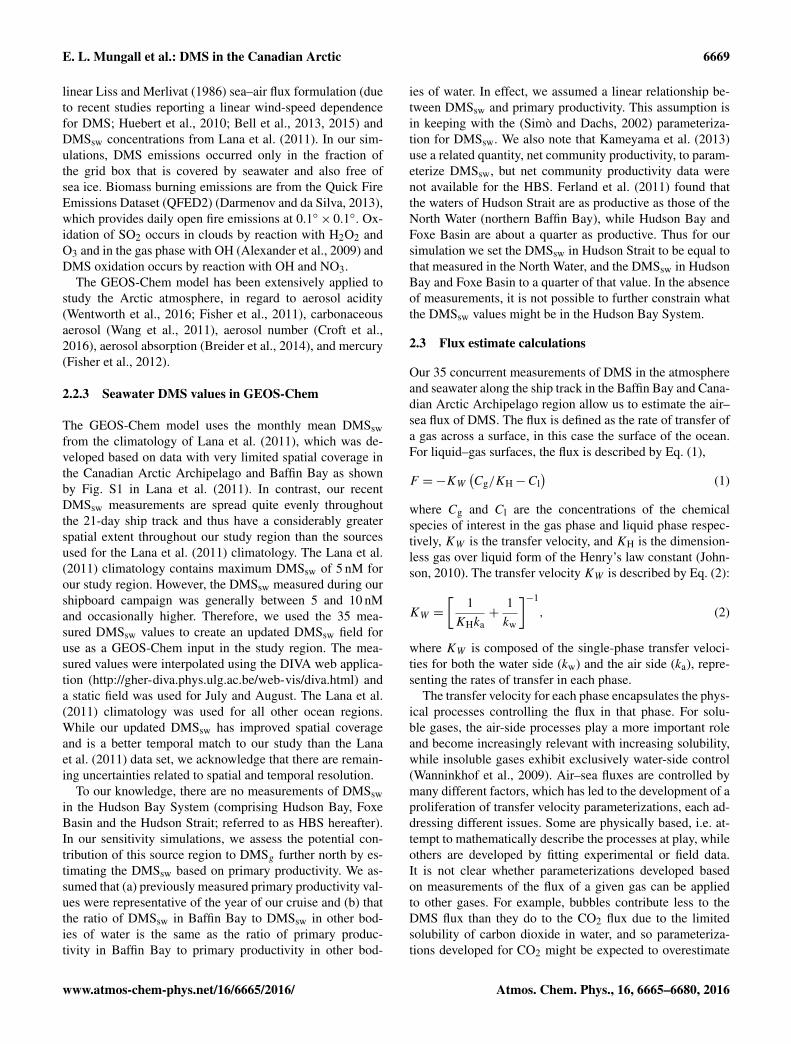
Figure 1. (a) The Amundsen ship position with dates indicated by colours. (b) Surface-layer atmospheric dimethyl sulfide (DMS) mix-ing ratios from ship-based high-resolution time-of-flight chemical ionization mass spectrometer (HR-ToF-CIMS) measurement with colourshowing magnitude of mixing ratios.

FLEXPART-WRF particle dispersion model, which exam-ine the potential contribution of seawater and non-marinesources to the measured DMSg .

2 Methods

2.1 Measurements

Measurements of DMS were made during the first leg of theCCGS Amundsen summer campaign under the aegis of NET-CARE (Network on Climate and Aerosols: Addressing Un-certainties in Remote Canadian Environments). The researchcruise started in Quebec City on 8 July 2014 and ended inKugluktuk on 14 August 2014. Measurements were made inBaffin Bay, Lancaster Sound, and Nares Strait. The ship trackis shown in Fig. 1a.

2.1.1 DMS mixing ratios

DMSg measurements were made using a high-resolutiontime-of-flight chemical ionization mass spectrometer (HR-ToF-CIMS, Aerodyne). The instrument was housed in a con-tainer on the foredeck. The inlet was placed on a tower9.44 m above the deck at the bow, which was itself nomi-nally 6.6 m above sea level (in total ca. 16 m a. s. l.). A di-aphragm pump pulled air at 30 L min−1 through a 25 m long,9.53 mm inner diameter PFA line heated to 50◦ (ClaybornLabs). Flow rate through the line was controlled by a criticalorifice. The flow was subsampled and pulled to the instru-ment inlet through another critical orifice restricting the flowto 2 L min−1. The flow through the sealed 210Po source of theHR-ToF-CIMS, also controlled at 2 L min−1 by a critical ori-fice, was supplied by a zero air generator (Parker Balston,

model HPZA-18000, followed by a Carbon Scrubber P/NB06-0263) via a mass flow controller supplying 2.4 L min−1.The zero air generator also supplied 9.8 sccm (controlled bya mass flow controller) through a bubbler filled with benzene,which was added to the flow through the radioactive sourceto provide the reagent ion. The excess went to exhaust. Fig-ure S1 in the Supplement shows a flow schematic.

The use of benzene cations as a reagent ion for chemicalionization mass spectrometry was first proposed by Allgoodet al. (1990). This reagent ion was successfully applied tothe shipboard detection of DMSg by Kim et al. (2016). Theionization mechanism that prevails is the transfer of chargefrom a benzene cation to an analyte ion which has an ioniza-tion energy lower than that of benzene (Allgood et al., 1990).Due to space constraints on board the ship, a zero air gen-erator was used instead of cylinder nitrogen to produce ourreagent ion flows. The use of zero air introduced other po-tential reagent ions to the mass spectrum (O+2 , NO+, C6H+7 ,and H2O·H3O+; shown in Fig. S2). To investigate the effectof this more complicated reagent ion source, calibration ex-periments were carried out in the laboratory prior to the cam-paign for both air and N2 at different sample flow relativehumidities and under different CIMS voltage configurations.The calibration curves for DMS (detected as CH3SCH+3 )showed a linear response under all conditions. We found thatthe sensitivity of the instrument to DMS did not depend onrelative humidity. The average sensitivity measured by one-point calibrations in the field (±1σ ) was 80± 30 cps pptv−1.Actual uncertainties on the calibration factor were less as atime-varying calibration factor was applied to the data, asdescribed below. Detection limits were below 4 pptv as thebackground was consistently 2–3 pptv.

www.atmos-chem-phys.net/16/6665/2016/ Atmos. Chem. Phys., 16, 6665–6680, 2016

6668 E. L. Mungall et al.: DMS in the Canadian Arctic

Background spectra were collected in the field by over-flowing the inlet with zero air from the zero air generatoras shown in Fig. S1. The high mass resolution of the instru-ment eliminated concern about unit mass isobaric interfer-ences as indicated in Fig. S3. Mass spectra were collectedat 10 Hz. One-point calibrations were performed nearly ev-ery day by overflowing the inlet with zero air and addinga known amount of DMS from a standards cylinder usinga mass flow controller (499± 5 % ppb, Apel-Reimer). Peakfitting was performed using the Tofware software packagefrom Aerodyne (version 2.4.4) in Igor Pro. Reported mixingratios were calculated by first normalizing analyte peak areasto reagent ion peak areas, then subtracting backgrounds, andfinally applying calibration factors obtained by linearly in-terpolating the one-point daily calibrations. Text S1 providesdetails. To remove artifacts that might have occurred due toenhanced DMS flux in the ship’s wake, the data were filteredsuch that values were removed when the ship was moving(speed over ground greater than 2 m s−1) and the wind direc-tion was not within ±90◦ of the bow. This filtering removedless than 12 % of data points.

2.1.2 Surface seawater DMS concentrations

Seawater concentrations of DMS were determined followingprocedures described by Scarratt et al. (2000) and modified inLizotte et al. (2012) using purging, cryotrapping, and sulfur-specific gas chromatography. Briefly, seawater was gentlycollected directly from 12 L Niskin bottles in gas-tight 24 mLserum vials, allowing the water to overflow. Subsamples ofDMS were withdrawn from the 24 mL serum vials withinminutes of collection and sparged using an in line purgeand trap system with a Varian 3800 gas chromatograph (GC)equipped with a pulsed flame photometric detector (PFPD).The GC was calibrated with injections of a 100 nM solutionof hydrolyzed DMSP (Research Plus Inc.). The full data setwill be presented separately (M. Lizotte, personal communi-cation, 2015).

2.1.3 Meteorological data

Basic meteorological measurements were made from a pur-pose built tower on the ship’s foredeck. Air temperature(8.2 m above deck), wind speed and direction (9.4 m abovedeck), and barometric pressure (1.5 m above deck) were mea-sured using respectively a shielded temperature and rela-tive humidity probe (Vaisala™ HMP45C212), wind monitor(RM Young 05103), and pressure transducer (RM Young™

61205V). Sensors were scanned every 2 s and saved as 2 minaverages to a micrologger (Campbell Scientific™, modelCR3000). Platform relative wind was post-processed to truewind following Smith et al. (1999). Navigation data (ship po-sition, speed over ground, course over ground, and heading)necessary for the conversion were available from the ship’sposition and orientation system (Applanix POS MV™ V4).

Periods when the tower sensors were serviced or when theplatform relative wind was beyond±90◦ from the ship’s bowwere screened from the meteorological data set. Screened pe-riods accounted for less than 20 % of total data but up to 45 %in some regions.

2.1.4 Sea surface temperature (SST) and salinity

SST was measured with the ship’s Inboard Shiptrack WaterSystem, Seabird/Seapoint measurement system. There wereno continuous salinity measurements. An average salinityvalue of 29.7 PSU was used for all calculations since the cal-culated transfer velocities had very low sensitivity to changesin salinity for our study region.

2.2 Model descriptions

2.2.1 FLEXPART-WRF

A Lagrangian particle dispersion model based on FLEX-PART (Stohl et al., 2005), FLEXPART-WRF (Brioudeet al., 2013, website: https://www.flexpart.eu/wiki/FpLimitedareaWrf), was used to study the origin of airsampled by the ship. The model is driven by meteorologyfrom the Weather Research and Forecasting (WRF) model(Skamarock et al., 2005) and was run in backward mode tostudy the emissions source regions and transport pathwaysinfluencing ship-based DMS measurements. Specific detailsare in Wentworth et al. (2016).

2.2.2 GEOS-Chem

The GEOS-Chem chemical transport model(www.geos-chem.org) was used to conduct source sen-sitivity studies. We used GEOS-Chem version 9-02 at2◦× 2.5◦ resolution with 47 vertical layers between thesurface and 0.01 hPa. The assimilated meteorology is takenfrom the National Aeronautics and Space Administration(NASA) Global Modeling and Assimilation Office (GMAO)Goddard Earth Observing System version 5.7.2 (GEOS-FP)assimilated meteorology product, which includes bothhourly surface fields and 3-hourly 3-D fields. Our simula-tions used 2014 meteorology and allowed a 2-month spin-upprior to the simulation of July and August 2014.

The GEOS-Chem model includes a detailed oxidant–aerosol tropospheric chemistry mechanism as originally de-scribed by Bey et al. (2001). Simulated aerosol species in-clude sulfate–nitrate–ammonium (Park et al., 2004, 2006),carbonaceous aerosols (Park et al., 2003; Liao et al., 2007),dust (Fairlie et al., 2007, 2010), and sea salt (Alexanderet al., 2005). The sulfate–nitrate–ammonium chemistry usesthe ISORROPIA II thermodynamic model (Fountoukis andNenes, 2007), which partitions ammonia and nitric acid be-tween the gas and aerosol phases. The model includes nat-ural and anthropogenic sources of SO2 and NH3 (Fisheret al., 2011). DMS emissions are based on the piece-wise

Atmos. Chem. Phys., 16, 6665–6680, 2016 www.atmos-chem-phys.net/16/6665/2016/

E. L. Mungall et al.: DMS in the Canadian Arctic 6669

linear Liss and Merlivat (1986) sea–air flux formulation (dueto recent studies reporting a linear wind-speed dependencefor DMS; Huebert et al., 2010; Bell et al., 2013, 2015) andDMSsw concentrations from Lana et al. (2011). In our sim-ulations, DMS emissions occurred only in the fraction ofthe grid box that is covered by seawater and also free ofsea ice. Biomass burning emissions are from the Quick FireEmissions Dataset (QFED2) (Darmenov and da Silva, 2013),which provides daily open fire emissions at 0.1◦× 0.1◦. Ox-idation of SO2 occurs in clouds by reaction with H2O2 andO3 and in the gas phase with OH (Alexander et al., 2009) andDMS oxidation occurs by reaction with OH and NO3.

The GEOS-Chem model has been extensively applied tostudy the Arctic atmosphere, in regard to aerosol acidity(Wentworth et al., 2016; Fisher et al., 2011), carbonaceousaerosol (Wang et al., 2011), aerosol number (Croft et al.,2016), aerosol absorption (Breider et al., 2014), and mercury(Fisher et al., 2012).

2.2.3 Seawater DMS values in GEOS-Chem

The GEOS-Chem model uses the monthly mean DMSswfrom the climatology of Lana et al. (2011), which was de-veloped based on data with very limited spatial coverage inthe Canadian Arctic Archipelago and Baffin Bay as shownby Fig. S1 in Lana et al. (2011). In contrast, our recentDMSsw measurements are spread quite evenly throughoutthe 21-day ship track and thus have a considerably greaterspatial extent throughout our study region than the sourcesused for the Lana et al. (2011) climatology. The Lana et al.(2011) climatology contains maximum DMSsw of 5 nM forour study region. However, the DMSsw measured during ourshipboard campaign was generally between 5 and 10 nMand occasionally higher. Therefore, we used the 35 mea-sured DMSsw values to create an updated DMSsw field foruse as a GEOS-Chem input in the study region. The mea-sured values were interpolated using the DIVA web applica-tion (http://gher-diva.phys.ulg.ac.be/web-vis/diva.html) anda static field was used for July and August. The Lana et al.(2011) climatology was used for all other ocean regions.While our updated DMSsw has improved spatial coverageand is a better temporal match to our study than the Lanaet al. (2011) data set, we acknowledge that there are remain-ing uncertainties related to spatial and temporal resolution.

To our knowledge, there are no measurements of DMSswin the Hudson Bay System (comprising Hudson Bay, FoxeBasin and the Hudson Strait; referred to as HBS hereafter).In our sensitivity simulations, we assess the potential con-tribution of this source region to DMSg further north by es-timating the DMSsw based on primary productivity. We as-sumed that (a) previously measured primary productivity val-ues were representative of the year of our cruise and (b) thatthe ratio of DMSsw in Baffin Bay to DMSsw in other bod-ies of water is the same as the ratio of primary produc-tivity in Baffin Bay to primary productivity in other bod-

ies of water. In effect, we assumed a linear relationship be-tween DMSsw and primary productivity. This assumption isin keeping with the (Simò and Dachs, 2002) parameteriza-tion for DMSsw. We also note that Kameyama et al. (2013)use a related quantity, net community productivity, to param-eterize DMSsw, but net community productivity data werenot available for the HBS. Ferland et al. (2011) found thatthe waters of Hudson Strait are as productive as those of theNorth Water (northern Baffin Bay), while Hudson Bay andFoxe Basin are about a quarter as productive. Thus for oursimulation we set the DMSsw in Hudson Strait to be equal tothat measured in the North Water, and the DMSsw in HudsonBay and Foxe Basin to a quarter of that value. In the absenceof measurements, it is not possible to further constrain whatthe DMSsw values might be in the Hudson Bay System.

2.3 Flux estimate calculations

Our 35 concurrent measurements of DMS in the atmosphereand seawater along the ship track in the Baffin Bay and Cana-dian Arctic Archipelago region allow us to estimate the air–sea flux of DMS. The flux is defined as the rate of transfer ofa gas across a surface, in this case the surface of the ocean.For liquid–gas surfaces, the flux is described by Eq. (1),

F =−KW(Cg/KH−Cl

)(1)

where Cg and Cl are the concentrations of the chemicalspecies of interest in the gas phase and liquid phase respec-tively, KW is the transfer velocity, and KH is the dimension-less gas over liquid form of the Henry’s law constant (John-son, 2010). The transfer velocityKW is described by Eq. (2):

KW =

[1

KHka+

1kw

]−1

, (2)

where KW is composed of the single-phase transfer veloci-ties for both the water side (kw) and the air side (ka), repre-senting the rates of transfer in each phase.

The transfer velocity for each phase encapsulates the phys-ical processes controlling the flux in that phase. For solu-ble gases, the air-side processes play a more important roleand become increasingly relevant with increasing solubility,while insoluble gases exhibit exclusively water-side control(Wanninkhof et al., 2009). Air–sea fluxes are controlled bymany different factors, which has led to the development of aproliferation of transfer velocity parameterizations, each ad-dressing different issues. Some are physically based, i.e. at-tempt to mathematically describe the processes at play, whileothers are developed by fitting experimental or field data.It is not clear whether parameterizations developed basedon measurements of the flux of a given gas can be appliedto other gases. For example, bubbles contribute less to theDMS flux than they do to the CO2 flux due to the limitedsolubility of carbon dioxide in water, and so parameteriza-tions developed for CO2 might be expected to overestimate

www.atmos-chem-phys.net/16/6665/2016/ Atmos. Chem. Phys., 16, 6665–6680, 2016

6670 E. L. Mungall et al.: DMS in the Canadian Arctic

Table 1. Summary of past DMS atmospheric mixing ratio measurements in the Arctic.

Study Leck and Persson(1996)

Rempillo et al. (2011) Rempillo et al. (2011) Chang et al. (2011) Tjernström et al.(2014)

This work

Cruise Name IAOE-91 Amundsen 2007 Amundsen 2008 Amundsen 2008 ASCOS 2008 Amundsen 2014

Season Autumn (August,September, October)

Autumn (Early Octo-ber)

Autumn (lateSeptember)

Autumn (end of Au-gust, September)

Autumn (August, be-ginning of Septem-ber)

Summer (late Julyand early August)

Location Central Arctic Ocean Western CanadianArctic

Eastern CanadianArctic

Eastern CanadianArctic

Central Arctic Ocean Eastern CanadianArctic

Method Gas chromatography Gas chromatography Gas chromatography Proton transferreaction massspectrometry

Proton transferreaction massspectrometry

Benzene chemicalionization massspectrometry

Measurementfrequency

392 samples in 64days

9 samples in 3 days 18 samples in 3 days 5 min 1 min 10 Hz

Median 25 (1.1) 10 (0.44) 30 (1.3) 65.9 26 185.825th percentile 11 (0.48) 41.2 15 117.875th percentile 53 (2.3) 98.9 50 262.5Minimum 1.1 (0.047) Below detection

(< 7 pptv)Below detection(< 7 pptv)

0.3 4.0 Below detection(< 4 pptv)

Maximum 380 (17) 30 (1.3) 94 (4.1) 474 158 1155

The studies of Leck and Persson (1996) and Rempillo et al. (2011) report concentrations in nmol m−3. For purposes of comparison, these have been converted to mixing ratios for an atmospheric pressure and temperature of101 kPa and 4◦ respectively. Original (published) concentration values are reported in parentheses following the calculated mixing ratios.

the DMS flux (Blomquist et al., 2006). Indeed, recent stud-ies have shown that the wind speed dependence of the DMStransfer velocity is close to linear (Huebert et al., 2010; Bellet al., 2013, 2015).

Fluxes were calculated according to Eq. (1) using thetransfer velocity parameterizations of Liss and Merlivat(1986) and Jeffery et al. (2010) for water side and air siderespectively (adjusted to the ambient seawater Schmidt num-ber of DMS; details are in Johnson, 2010). Atmosphericconcentrations were calculated from measured mixing ra-tios using measured atmospheric temperature, pressure, andthe Henry’s law constant for DMS at the in situ tempera-ture. Fluxes were multiplied by the fraction of open waterin order to account for the capping effect of sea ice (Looseet al., 2014). The sea ice cover near the ship’s location wasestimated at a 0.5◦× 0.5◦ resolution by plotting the ship’scourse at hourly resolution on daily ice charts obtained fromthe Canadian Ice Service (http://www.ec.gc.ca/glaces-ice/).These estimates were cross-referenced with daily photostaken aboard the ship to ensure accuracy. Estimates weremade on a scale from 1 to 10 with no fractional values.

3 DMS mixing ratio observations and estimated fluxes

Figure 1b and Table 1 present the DMSg mixing ratio datacollected along the ship track. To our knowledge, these arethe first DMSg measurements for the Arctic during midsum-mer (July). These summertime measurements exceed previ-ous measurements made in late summer and early autumnby a factor of 3–10 (Table 1). This is consistent with theexpectation of higher biological productivity in the summerthan in other seasons (Levasseur, 2013). The time series ex-hibits high temporal variability. Three episodes of elevatedDMSg mixing ratios with values of 400 pptv or above oc-

curred along the ship track on 18–20, 26 July, and 1–2 Au-gust. Two episodes with DMSg mixing ratios with valuesbelow 100 pptv occurred on 22–23 July and 5 August. Ourvalues are on the same order (hundreds of pptv) as mea-surements made at high latitudes under bloom conditions inthe Southern Ocean (Bell et al., 2015; Yang et al., 2011),the North Atlantic (Bell et al., 2013), and the northwesternPacific (Tanimoto et al., 2013) but are higher than measure-ments made in the Tropical Pacific that were on the order oftens of pptv (Simpson et al., 2014).

Figure 2 presents the time series of DMSg along the shiptrack together with both measured and GEOS wind speeds,DMSsw, and our flux estimates. Previous DMS flux estimatesfor the Arctic are summarized in Table 2. The only othersummertime estimate falls within the same range as in thiswork of ca. 0–10 µmol day−1 m−2 (Sharma et al., 1999b). Abetter constrained summer flux estimate for this region willrequire sampling of DMSsw at higher spatial and temporalresolution, and ideally direct continuous flux measurementsusing a technique such as eddy covariance, but these are chal-lenging measurements rendered more so by the remotenessof Arctic Ocean.

4 Source sensitivity studies with GEOS-Chem andFLEXPART

In order to explore the provenance of the air masses beingsampled on the ship, we used FLEXPART-WRF backwardruns as well as GEOS-Chem simulations. Figure 3 summa-rizes our understanding of the origins of air masses arrivingat the ship track. Figure 3a shows the time series of DMSgfrom the GEOS-Chem simulation superimposed on the mea-sured DMSg time series, as well as the GEOS-Chem sea salt(a marine tracer) and methyl ethyl ketone and carbon monox-

Atmos. Chem. Phys., 16, 6665–6680, 2016 www.atmos-chem-phys.net/16/6665/2016/

E. L. Mungall et al.: DMS in the Canadian Arctic 6671

Figure 2. Time series along Amundsen ship track of (a) atmospheric DMS mixing ratio (10 Hz) from HR-ToF-CIMS, (b) observed DMSsurface seawater concentration, (c) hourly-averaged wind speed at ship position (black) and hourly-average GEOS wind speed at ship position(red), and (d) DMS water-air flux estimates.

Table 2. Summary of previous air–ocean DMS flux values in the Arctic.

Flux Date Location Method Authors

0.02–12 µmol m−2 d−1 Summer 2014 (July andAugust)

Eastern Canadian Arctic Estimated frommeasurements

This work

0.1–2.6 µmol m−2 d−1 Autumn 2007, 2008(September to November)

Beaufort Sea to Baffin baythrough Lancaster Sound

Estimated frommeasurements

(Rempillo et al., 2011)

0.002–8.4 µmol m−2 d−1 Autumn 1991 (August toOctober)

Central Arctic Ocean andGreenland Sea

Estimated frommeasurements

(Leck and Persson, 1996)

0.007–11.5 µmol m−2 d−1 Summer 1994 (July andAugust)

Central Arctic Ocean east–west transect

Estimated frommeasurements

(Sharma et al., 1999b)

0.5 µmol m−2 d−1 January North of 60◦ N Global model (Erickson et al., 1990)4–12 µmol m−2 d−1 March–December 1996 Gulf of Alaska Regional model (Jodwalis et al., 2000)

ide (MEK and CO, biomass burning tracers) mixing ratios.Figure 3b shows the main land cover types in the region.Figure 3c shows examples of potential emissions sensitivity(PES) plots generated using FLEXPART-WRF that indicateregions the air has passed over before being sampled. Periodshighlighted with a grey bar and numbered 1 through 3 werechosen as representative of three types of influence: (1) ma-rine influence from south of the Arctic circle, (2) terrestrialinfluence from northern Canada, and (3) regional marine in-fluence from Baffin Bay. Sea salt tracer maxima indicatemarine-influenced air and reflect high winds, while MEKand CO maxima indicate an influence from biomass burning.Biomass burning tracers provide a convenient indication ofcontinental influence on the air mass. Figure 3 shows agree-ment between the sources of the air indicated by FLEXPART-WRF and by the GEOS-Chem tracers. For example, dur-ing Period 2 the MEK tracer is high and FLEXPART-WRF

shows continental influence, while during Period 3 the seasalt tracer is high and FLEXPART-WRF shows marine influ-ence.

4.1 Model–measurement comparison

In comparing the simulated DMSg to our measurements, weassumed that the major cause of discrepancies between mea-surements and model was the representation of the DMSsource in GEOS-Chem. Essentially, since the GEOS-Chemmodel has realistic capabilities in the simulation of transport(Kristiansen et al., 2016) and the chemical sinks of DMS arerelatively well understood (Barnes et al., 2006), we choseto keep the transport and sink parameterizations constant forour sensitivity studies and focused on source sensitivity stud-ies due to the considerable source-related uncertainty.

Figure 3a shows that our GEOS-Chem simulations repro-duce the major features of the measured DMSg time series,

www.atmos-chem-phys.net/16/6665/2016/ Atmos. Chem. Phys., 16, 6665–6680, 2016

6672 E. L. Mungall et al.: DMS in the Canadian Arctic

Figure 3. (a) Surface-layer atmospheric time series along Amundsen ship track of (a) measured and GEOS-Chem (GC) simulated DMS;(b) GC simulation of accumulation mode sea salt mass concentration; (c) GC simulation of methyl ethyl ketone (MEK) mixing ratio; (d) GCsimulation of carbon monoxide (CO) mixing ratio. (b) Olson Land Cover map of North America showing low-lying tundra (red), other tundra(grey), forest (green), wetlands and marsh (brown), and inland water (dark blue). (c) FLEXPART-WRF potential emissions sensitivity (PES)simulation plots showing the likely origin of the air mass at the ship position. The colour scale in seconds corresponds to time spent in thelower 300–1000 m (marked on each plot) before arriving at the ship position. The three plots correspond to the three periods shown by thenumbers and shaded bars in (a), showing examples of (1) transport from lower latitudes, including Hudson Bay (2) continentally influencedair (3) local marine influence from Baffin Bay.

with appropriate magnitudes much of the time and an over-all bias of−67 pptv. The poorest model–measurement agree-ments occur on 1–2 and 6–7 August, as shown in Figs. 4band 3a, where GEOS-Chem overestimates DMS mixing ra-tios by a factor of 2–3. This overestimation coincides withhigh levels of the accumulation mode sea salt aerosol tracerin GEOS-Chem as shown in Fig. 3b. The overestimation maybe due simulation errors related to the DMSsw field, exces-sive GEOS wind speeds driving too large of a flux duringthis episode, or the performance of the air–sea transfer veloc-ity parameterization at high wind speeds. Wind speeds in ourGEOS-Chem simulations display considerable scatter aboutthe observed wind speeds along the ship-track time series butshow a linear relationship with a slope of 0.95 and R2

= 0.35as in Fig. S4 and reproduce major features of the wind timeseries as in Fig. 2c. Overall, GEOS-Chem tended to overes-timate DMSg in Baffin Bay (largely open water at the timeof the campaign) and underestimate it in Lancaster Sound

(where we encountered between 10 and 100 % ice cover). Itis worth noting that the effect of sea ice on sea–air flux ashypothesized by Loose et al. (2014) is to increase the flux atlow wind speeds and decrease it at high wind speeds. Imple-mentation of this transfer velocity parameterization might beexpected to improve model–measurement agreement. Morework is needed to assess how best to parameterize air–seaflux in high-latitude regions and the marginal ice zone in par-ticular. Within these uncertainties, the seawater DMS sourcecould largely account for the measured DMSg . However,there are some notable mismatches that cannot be accountedfor by the uncertainties detailed above. These are discussedin the following sections.

Atmos. Chem. Phys., 16, 6665–6680, 2016 www.atmos-chem-phys.net/16/6665/2016/

E. L. Mungall et al.: DMS in the Canadian Arctic 6673

Figure 4. (a) GEOS-Chem (GC) simulated atmospheric surface-layer DMS mixing ratio along Amundsen ship track as in Fig. 3a, with indi-cation of contributions from Baffin Bay (blue), from Lancaster Sound (purple), and from other marine regions (red). (b) Difference betweenmeasurement and simulated DMS mixing ratio time series along the ship track showing model overprediction in blue and underprediction inorange. (c) GC simulated DMS contributions along ship track from sensitivity tests for additional DMS sources such as melt ponds (blue),tundra (brown), and unknown sources possibly including forests, soils, or lakes in proximity to biomass burning (green).

4.2 Seawater sources: Baffin Bay and Lancaster Soundas principal oceanic DMS source

Our model–measurement comparisons suggest that as ex-pected, seawater makes the dominant contribution to themeasured DMSg . In this section, we examine the potentialregional contributions. Figure 4a shows the relative contribu-tions of various marine source regions to the GEOS-Chemsimulation of the DMSg along the ship track. Nearly 90 % ofthe simulated DMSg could be explained by the DMS oceanicemissions from Baffin Bay and Lancaster Sound when usingthe DMSsw field based on our in situ measurements. The sim-ulated DMSg values originating from Baffin Bay and Lan-caster Sound are shown in blue and purple respectively inFig. 4a. These local emissions also contributed the majorityof the highest mixing ratios observed during the campaign on18 and 20 July. Overall, we conclude that the waters of Baf-fin Bay and Lancaster Sound acted as a strong local sourceof DMSg throughout the campaign.

4.3 Transport from a seawater source: role of HudsonBay System as an additional oceanic DMS source

Figure 4 shows that the simulated influence of the HBS is sig-nificant on 18–19 July, contributing up to 60 % of simulatedDMSg towards the end of that time period. This peak in DMScoincided with a synoptic-scale storm system, which orig-inated at lower latitudes and passed over Lancaster Sound,where the ship was located at the time. This transport patternis visible in the FLEXPART-WRF retroplume for Period 1in Fig. 3c. These results suggest that DMS emissions from

the HBS are potentially an important source of atmosphericsulfur to the Arctic atmosphere during episodic transportevents associated with mid-latitude storms travelling north-ward. Our simulated results depend on the assumption thatthe DMSsw values in the HBS are similar to those observedat higher latitudes. The potential for influence from the HBSis supported by previous reports of high levels of DMSg inair masses transported northward from the Hudson Bay re-gion (Sjostedt et al., 2012). Measurements of both DMSswand DMSg in the HBS are needed to confirm this hypothesis.

4.4 Investigation of possible missing sources

The GEOS-Chem simulated DMSg time series underesti-mates the peaks in measured DMSg on 17 and 26 July(shown in Fig. 3a). This mismatch coincides with a min-imum in the simulated marine tracer (sea salt), suggestingthat possibly a non-marine source of DMSg is not being rep-resented in the GEOS-Chem DMS parameterization. Sincethe emissions of DMSg and sea salt aerosol are similarly de-pendent on wind speed and fraction of open ocean and theirlifetimes are similarly short, we expect the DMSg and seasalt tracers in our simulation to covary when the DMSg isof marine origin. We note that the GEOS wind speeds arein good agreement with measured wind speeds during thesetime periods, as shown in Fig. 2c. It is possible that thismodel–measurement disagreement indicates that the modeldoes not capture the true relationship of DMSg to wind speedor that the GEOS-Chem simulation is missing a coastal bodyof water at a sub-grid scale and that this water body wasemitting large quantities of DMS. However, the FLEXPART-

www.atmos-chem-phys.net/16/6665/2016/ Atmos. Chem. Phys., 16, 6665–6680, 2016

6674 E. L. Mungall et al.: DMS in the Canadian Arctic

WRF retroplumes for 26 July (an example is shown as Period2 of Fig. 3c) indicate that the air mass had spent most of itstime over land surfaces and sea ice before reaching the ship’slocation. This continental air-mass origin is further supportedby high levels of simulated continental tracers (e.g. MEK,shown in the third panel of Fig. 3a) during these same peri-ods.

The suggestion that DMSg may have a continental sourceis not new (Hopke et al., 1995), but it has not received verymuch attention. The FLEXPART-WRF PES retroplumes in-dicate that the continental area influencing the air massessampled by the ship was northern Canada (primarily, regionsto the south and east of Baffin Bay, including Nunavut andthe Northwest Territories). The land cover in that region isshown in Fig. 3b and is a mixture of tundra, boreal forest,wetlands, and lakes. As well, there was a wide spatial ex-tent of melt ponds to the south and west of the ship track(shown in Fig. S5). To investigate the impact that each ofthese sources could have had on the DMSg measured duringthe campaign, we estimated the DMS emission potential ofeach land cover type (including melt ponds) based on exist-ing literature values. We implemented these extra emissionsin the GEOS-Chem model and performed sensitivity tests toexplore their potential to make additional contributions toDMSg at the ship positions. These results are presented inthe following subsections.

4.4.1 Emissions from melt ponds

Melt ponds form on the surface of sea ice as the snowmelts.They cover much of the surface of the sea ice by mid-summerand have been suggested as a potentially important source ofDMS to the atmosphere (Levasseur, 2013). At the time ofthe campaign, the sea ice regions to the west and south ofour ship track, particularly in Lancaster Sound, had consid-erable melt pond coverage as shown in Fig. S5. The meltpond DMS source was implemented in GEOS-Chem by as-suming that 50 % of sea ice was covered by melt ponds andtreating melt ponds as seawater with a DMSsw concentrationof 3 nM (expected to be an upper limit based on Levasseur(2013). The Liss and Merlivat (1986) transfer velocity pa-rameterization was used. The validity of assuming the sameflux parameterization applies to a shallow melt pond as to theopen ocean is untested, but it is a reasonable approximationfor our sensitivity test.

The blue curve in Fig. 4c shows the simulated DMSg con-tribution for the melt pond source. The simulated melt pondcontribution was greatest during 18–25 July when the shipwas in Lancaster Sound. The maximum simulated melt pondcontribution was about 100 % on 23 July when simulatedand measured DMSg were very low. The strong contribu-tion of the melt ponds at this time was likely due to theship’s position at the ice edge and advection of the arriv-ing air mass over ice-covered regions. The simulated meltpond source contributed an average about 20 % to the total

simulated DMSg over the remainder of the time series. Im-plementation of this source reduced the overall normalizedmean model–measurement bias by 9 %, suggesting that meltponds could serve to elevate the regional background levelsof DMSg . Further measurements of DMS concentrations inmelt ponds and, ideally, direct measurements of DMS fluxesfrom melt ponds are needed to better constrain the impactthis source might have on DMSg in the Arctic summer.

4.4.2 Emissions from coastal tundra

Previous studies suggest that DMS emissions from lichens(Gries et al., 1994) and from coastal tundra, particularly inregions where snow geese breed (Hines and Morrison, 1992),may be quite large. For lichens to emit reduced sulfur to theatmosphere, they require a source of sulfur. In coastal regionsthis can be supplied by sea spray. We implemented a tundraDMS source in GEOS-Chem by using the Olson Land Coverdata (http://edc2.usgs.gov/glcc/globdoc2_0.php) to calculatethe fraction of each GEOS-Chem grid box covered by theland type “barren tundra”. We then assumed that 40 % ofthat tundra (to account for inland regions emitting less dueto less sulfate being deposited by sea spray) emitted DMS ata rate of 480 nM m−2 h−1 (Hines and Morrison, 1992). Weconsider this simulation to give us an upper limit to the po-tential influence of tundra DMS emissions.

The results are presented as the brown curve in Fig. 4c.The simulated DMSg at the ship track had the largest contri-bution from tundra sources during 16–17 July, with a max-imum contribution to the simulated DMSg at the ship po-sition of 6 %. The percent contribution was lower than thatof the melt pond source because the tundra source acted toincrease simulated DMSg during times when levels were al-ready high, but as can be seen in Fig. 4c the absolute contri-bution of the simulated tundra source was comparable to orgreater than the melt pond source contribution. Like the meltpond source, the possible tundra source reduces the overallnormalized mean bias (by 14 %) and may contribute to the re-gional background levels of DMSg . However, neither sourcecan account for the large unexplained peaks in the measuredtime series.

4.4.3 Emissions from lakes

To evaluate the potential contribution of DMS from lakes,the fresh water fraction in each GEOS-Chem grid box ina rectangular domain spanning 48 to 75◦ N and −68 to−140◦W was calculated using the Olson Land Cover map, at1 km× 1 km resolution. Based on the work of Sharma et al.(1999a), we assigned a mean value of 1 nM DMS to thefresh water in that domain. We then applied the same Lissand Merlivat (1986) parameterization to the fraction of thegrid box with lake coverage. The same caveats apply to theuse of transfer velocity parameterizations developed for theopen ocean for fluxes from lakes as to the application to melt

Atmos. Chem. Phys., 16, 6665–6680, 2016 www.atmos-chem-phys.net/16/6665/2016/

E. L. Mungall et al.: DMS in the Canadian Arctic 6675

Figure 5. (a) GEOS-Chem simulated July mean surface-layer atmospheric DMS in Canada; (b) absolute change in simulated surface-layerDMS with implementation of lake DMS emissions; (c) percent change in simulated Canadian surface-layer DMS due to DMS emissionsfrom wildfires; (d) percent changes in simulated surface-layer DMS with the implementation of lake DMS emissions.

ponds as discussed above. In our simulation, the lake sourcewas only locally important as shown in Fig. 5. There was amodest contribution to the absolute magnitude of DMSg innorthern Quebec and Labrador, but the simulation showednegligible effects of the lake source on surface-layer DMSgelsewhere. The percent change in surface-layer DMSg in theNorthwest Territories was quite large due to there being noother simulated sources of DMSg in that location, but theabsolute values of DMSg are very small. However, as thereare few measurements of DMS concentrations in lakes innorthern Canada, we cannot exclude the possibility that theactual lake concentrations of DMSsw are much higher than1 nM and that the unexplained peak in our time series is dueto a lake source of DMSg . This possibility is supported byhigh chlorophyll-α levels in the lakes of northern Canada(shown in Fig. S6) and the fact that the measurements ofDMSsw in lakes that we used for this sensitivity test weremade more than 15 years ago, and the high northern latitudeshave warmed significantly since then (IPCC, 2013).

4.4.4 Other potential DMS sources for the study area

Due to the paucity of measurements of DMS emissions fromvegetation, boreal soils, and Arctic wetlands, especially dur-ing and in proximity to biomass burning events, this po-tential missing source is very difficult to evaluate. The cor-relation between the measurement–model residual and the

biomass burning tracers in GEOS-Chem shown in Fig. 3asuggests that DMSg was being co-transported with thesebiomass burning tracers. The measurement–model differenceand the MEK tracer have a similar peak on 26 July as shownin Fig. 3a. The FLEXPART-WRF retroplumes (e.g. Period 2in Fig. 3) identify this time as being continentally influenced.

DMS emissions have been reported from biomass burn-ing (Akagi et al., 2011; Meinardi et al., 2003). Summer 2014was a particularly active wildfire season in northern Canada(Blunden and Arndt, 2015). The simplest reason for the max-ima in biomass burning tracers during the unexplained DMSgpeak on 26 July would be emissions of DMS from biomassburning that are not represented in the model. To gauge theimportance of this source to DMSg in the Arctic, we used theemission factor for DMS from boreal forest biomass burn-ing reported by Akagi et al. (2011). We indexed the simu-lated DMS emissions to CO emissions, such that 3.66×10−5

molecules of DMS are emitted for each molecule of CO emit-ted. Figure 5 shows that the biomass burning sensitivity testindicated that the biomass burning source of DMSg had lo-cal influence only, like the modelled lake source. The rea-son for this is that the emission factor for DMS from borealforest fires is not very large. As a result, this source actedto increase DMSg in the immediate vicinity of the wildfiresin the Northwest Territories but had a negligible influenceon the time series and is therefore not shown in Fig. 4. Thebiomass burning source of DMSg was likely not sufficient

www.atmos-chem-phys.net/16/6665/2016/ Atmos. Chem. Phys., 16, 6665–6680, 2016

6676 E. L. Mungall et al.: DMS in the Canadian Arctic

to directly influence the DMSg time series at the ship posi-tion, unless the emission factor used in the model is an or-der of magnitude too low. This seems unlikely as the emis-sion factor we used was derived from direct measurementsin a biomass burning plume originating from the boreal for-est (Akagi et al., 2011). Considerably larger DMS emissionshave been measured from other types of biomass burning inother locations (Meinardi et al., 2003) but we have no mea-surement evidence to support a higher emissions factor inour present simulations. We note that, in particular, emissionsfrom tundra fires are completely unconstrained and might bequite different from emissions from boreal forest fires due todifferent vegetation types and different types of burning (e.g.open flames versus smoldering). Further study is required.

Although the available information suggests that directDMS emissions from fires seem unlikely to explain thebias, support for the hypothesis that DMSg is being co-transported with biomass burning tracers is given by im-proved model–measurement agreement indicated by Fig. 3cif we assume the biomass burning plume contains equalamounts of DMSg and MEK and add this DMSg “source”to the simulated DMSg . This revision reduces the overallmeasurement–model bias by 24 % and reduces the residualby 200 pptv for the 26 July. Alternatively, the air mass ob-served at the ship could have passed over a strong near-landmarine source, which is missing in our simulations. However,the FLEXPART-WRF simulation indicates that the air masshad travelled over nearly entirely ice-covered regions beforearriving at the ship, suggesting that a marine source is a lesslikely explanation for the observed DMSg .

Emissions of reduced sulfur species from both soils andlakes are temperature dependent (Bates et al., 1992), sug-gesting that the wild fires could indirectly promote DMSemissions. Proximity to wild fires could increase the temper-ature of the soil as well as changing the air quality, whichmight stress biota. A mechanism whereby biomass burn-ing increases the emission of reduced sulfur species such asDMS from soils, lakes, and vegetation might yield increasedemissions but this requires further study and we do not haveany information that would allow implementation of this pos-sible effect in our simulations.

5 Conclusions

This study presents, to the best of our knowledge, the firstmeasurements of gaseous DMS mixing ratios in the sum-mertime Arctic atmosphere of Baffin Bay and parts of theCanadian Arctic Archipelago. Measured DMSg values weregreater than those measured in fall in the same region (con-sistent with higher biological productivity in summer) andbroadly consistent with measurements in other parts of theocean. We made flux estimates that fall within the rangeof existing DMS air–sea flux estimates for the summertimeCentral Arctic Ocean. The data presented here improve our

knowledge of atmospheric DMS levels in the summertimeArctic, but further study is needed to understand spatial, sea-sonal, and interannual variability of DMS both in the oceanand in the atmosphere.

We conducted sensitivity simulations with the GEOS-Chem chemical transport model to examine the potentialof various sources to contribute to DMSg measured alongthe ship track. We found that local oceanic sources can ac-count for a large proportion (70 % overall) of the atmosphericsurface-layer DMS measured along our ship track in theCanadian Arctic Archipelago and Baffin Bay during sum-mer 2014. Our GEOS-Chem simulations indicated that dur-ing transport events associated with synoptic-scale storms,marine sources south of the Arctic Circle made strong andepisodic contributions (as much as 60 %) to DMS mixingratios in the Canadian Arctic Archipelago region. The roleof transport in controlling DMS levels and the potential foraerosol particle formation from DMSg has been argued con-vincingly in a global sense by Quinn and Bates (2011). Wepropose that it may also be important episodically in the Arc-tic, e.g. transport from the Hudson Bay System or the North-west Territories. These origins for air at our ship track arealso supported by FLEXPART-WRF retroplume analysis.

GEOS-Chem simulations were biased low by 67 pptvover the ship-track time series (representing between 10and 100 % of the measured mixing ratios). We investigatedseveral additional sources (tundra, forests, lakes, and meltponds), which could contribute to surface-layer DMS mixingratios. Our sensitivity simulations indicated maximum con-tributions of 6 and 100 % from tundra and melt ponds respec-tively to the simulated total DMSg for the ship-track time se-ries, suggesting that emissions of DMS from melt ponds andcoastal tundra could have important local, regional effectson DMS levels. These sensitivity studies also suggest thatterrestrial or near-terrestrial sources could make additionalcontributions to DMSg in our study region. These emissionsmay be related to changes in lake, forest, and soil emissionsdue to the heat and stress associated with biomass burning.Flux measurements from melt ponds and the boreal forestand lakes, particularly when under stress from biomass burn-ing events, are needed to evaluate this hypothesis.

Our findings have implications for our understanding ofthe sulfur cycle in the summer Arctic and how it has changedin the recent past and will continue to change in the future.For example, much of the discussion surrounding changes inArctic DMS has focused on the loss of sea ice (Levasseur,2013), but the loss of permafrost might also have a large im-pact through changing nutrient levels in lakes (Rhüland andSmol, 1998). The potential influence of the observed atmo-spheric levels of DMS on new particle formation and subse-quent growth remains to be explored.

The Supplement related to this article is available onlineat doi:10.5194/acp-16-6665-2016-supplement.

Atmos. Chem. Phys., 16, 6665–6680, 2016 www.atmos-chem-phys.net/16/6665/2016/

E. L. Mungall et al.: DMS in the Canadian Arctic 6677

Author contributions. J. Abbatt and M. Levasseur designed the ex-periments and E. Mungall and M. Lizotte carried them out. J.Murphy, J. Liggio and J. Wentzell facilitated the Amundsen cam-paign. B. Croft and J. Thomas performed the GEOS-Chem andFLEXPART-WRF simulations respectively. E. Mungall carried outthe analysis, and E. Mungall prepared the manuscript with the aidof B. Croft and contributions from all co-authors.

Acknowledgements. The authors would like to acknowledge thefinancial support of NSERC for the NETCARE project fundedunder the Climate Change and Atmospheric Research program.As well, we thank ArcticNet for hosting NETCARE scientists onthe Amundsen, in particular the help of Keith Levesque, and allof the crew and scientists aboard. Additionally, special thanks toAmir Aliabadi, Ralf Staebler, Lauren Candlish, Heather Stark,Tonya Burgers, and Tim Papakyriakou for ozone sondes andmeteorological data. Thanks to Michelle Kim and Tim Bertramof UCSD for invaluable discussions of ion chemistry. The authorsthank K. Tavis and P. Kim for their assistance in implementation ofthe QFED2 database.

Edited by: A. Perring

References

Akagi, S. K., Yokelson, R. J., Wiedinmyer, C., Alvarado, M. J.,Reid, J. S., Karl, T., Crounse, J. D., and Wennberg, P. O.: Emis-sion factors for open and domestic biomass burning for usein atmospheric models, Atmos. Chem. Phys., 11, 4039–4072,doi:10.5194/acp-11-4039-2011, 2011.

Albrecht, B. A.: Aerosols, cloud microphysics, and fractionalcloudiness, Science, 245, 1227–1230, 1989.

Alexander, B., Park, R. J., Jacob, D. J., Li, Q., Yantosca, R. M.,Savarino, J., Lee, C., and Thiemens, M.: Sulfate formation insea-salt aerosols: Constraints from oxygen isotopes, J. Geophys.Res.-Atmos., 110, D10307, doi:10.1029/2004JD005659, 2005.

Alexander, B., Park, R. J., Jacob, D. J., and Gong, S.: Transitionmetal-catalyzed oxidation of atmospheric sulfur: Global impli-cations for the sulfur budget, J. Geophys. Res.-Atmos., 114,D02309, doi:10.1029/2008JD010486, 2009.

Allgood, C., Lin, Y., Ma, Y.-C., and Munson, B.: Benzene as a se-lective chemical ionization reagent gas, Org. Mass Spectrom.,25, 497–502, doi:10.1002/oms.1210251003, 1990.

Barnes, I., Hjorth, J., and Mihalopoulos, N.: Dimethyl Sulfide andDimethyl Sulfoxide and Their Oxidation in the Atmosphere,Chem. Rev., 106, 940–975, doi:10.1021/cr020529+, 2006.

Bates, T. S., Lamb, B. K., Guenther, A., Dignon, J., and Stoiber,R. E.: Sulfur emissions to the atmosphere from natural sourees,J. Atmos. Chem., 14, 315–337, doi:10.1007/BF00115242, 1992.

Bell, T. G., De Bruyn, W., Miller, S. D., Ward, B., Christensen,K. H., and Saltzman, E. S.: Air-sea dimethylsulfide (DMS) gastransfer in the North Atlantic: evidence for limited interfacial gasexchange at high wind speed, Atmos. Chem. Phys., 13, 11073–11087, doi:10.5194/acp-13-11073-2013, 2013.

Bell, T. G., De Bruyn, W., Marandino, C. A., Miller, S. D., Law,C. S., Smith, M. J., and Saltzman, E. S.: Dimethylsulfide gas

transfer coefficients from algal blooms in the Southern Ocean,Atmos. Chem. Phys., 15, 1783–1794, doi:10.5194/acp-15-1783-2015, 2015.

Bey, I., Jacob, D. J., Yantosca, R. M., Logan, J. A., Field, B. D.,Fiore, A. M., Li, Q., Liu, H. Y., Mickley, L. J., and Schultz,M. G.: Global modeling of tropospheric chemistry with as-similated meteorology: Model description and evaluation, 106,23073–23095, doi:10.1029/2001JD000807, 2001.

Blomquist, B. W., Fairall, C. W., Huebert, B. J., Kieber, D. J.,and Westby, G. R.: DMS sea-air transfer velocity: Direct mea-surements by eddy covariance and parameterization based onthe NOAA/COARE gas transfer model, Geophys. Res. Lett., 33,L07601, doi:10.1029/2006GL025735, 2006.

Blunden, J. and Arndt, D. S.: State of the Climatein 2014, B. Am. Meteorol. Soc., 96, ES1–ES32,doi:10.1175/2015BAMSStateoftheClimate.1, 2015.

Breider, T. J., Mickley, L. J., Jacob, D. J., Wang, Q., Fisher, J. A.,Chang, R. Y.-W., and Alexander, B.: Annual distributions andsources of Arctic aerosol components, aerosol optical depth, andaerosol absorption, J. Geophys. Res.-Atmos., 119, 4107–4124,doi:10.1002/2013JD020996, 2014.

Brioude, J., Arnold, D., Stohl, A., Cassiani, M., Morton, D.,Seibert, P., Angevine, W., Evan, S., Dingwell, A., Fast, J. D.,Easter, R. C., Pisso, I., Burkhart, J., and Wotawa, G.: The La-grangian particle dispersion model FLEXPART-WRF version3.1, Geosci. Model Dev., 6, 1889–1904, doi:10.5194/gmd-6-1889-2013, 2013.

Browse, J., Carslaw, K. S., Arnold, S. R., Pringle, K., and Boucher,O.: The scavenging processes controlling the seasonal cycle inArctic sulphate and black carbon aerosol, Atmos. Chem. Phys.,12, 6775–6798, doi:10.5194/acp-12-6775-2012, 2012.

Carslaw, K. S., Lee, L. A., Reddington, C. L., Pringle, K. J., Rap,A., Forster, P. M., Mann, G. W., Spracklen, D. V., Woodhouse,M. T., Regayre, L. A., and Pierce, J. R.: Large contribution ofnatural aerosols to uncertainty in indirect forcing, Nature, 503,67–71, doi:10.1038/nature12674, 2013.

Chang, R. Y.-W., Sjostedt, S. J., Pierce, J. R., Papakyriakou, T. N.,Scarratt, M. G., Michaud, S., Levasseur, M., Leaitch, W. R., andAbbatt, J. P. D.: Relating atmospheric and oceanic DMS levelsto particle nucleation events in the Canadian Arctic, J. Geophys.Res.-Atmos., 116, D00S03, doi:10.1029/2011JD015926, 2011.

Charlson, R. J., Lovelock, J. E., Andreae, M. O., and Warren, S. G.:Oceanic phytoplankton, atmospheric sulphur, cloud albedo andclimate, Nature, 326, 655–661, doi:10.1038/326655a0, 1987.

Chen, H., Ezell, M. J., Arquero, K. D., Varner, M. E., Dawson,M. L., Gerber, R. B., and Finlayson-Pitts, B. J.: New parti-cle formation and growth from methanesulfonic acid, trimethy-lamine and water, Phys. Chem. Chem. Phys., 17, 13699,doi:10.1039/C5CP00838G, 2015.

Croft, B., Martin, R. V., Leaitch, W. R., Tunved, P., Breider, T. J.,D’Andrea, S. D., and Pierce, J. R.: Processes controlling theannual cycle of Arctic aerosol number and size distributions,Atmos. Chem. Phys., 16, 3665–3682, doi:10.5194/acp-16-3665-2016, 2016.

Darmenov, A. and da Silva, A.: The quick fire emissions dataset(QFED)–documentation of versions 2.1, 2.2 and 2.4, NASATechnical Report Series on Global Modeling and Data Assimi-lation, NASA TM-2013-104606, 32, 183, 2013.

www.atmos-chem-phys.net/16/6665/2016/ Atmos. Chem. Phys., 16, 6665–6680, 2016

6678 E. L. Mungall et al.: DMS in the Canadian Arctic

Erickson, D. J., Ghan, S. J., and Penner, J. E.: Global ocean-to-atmosphere dimethyl sulfide flux, J. Geophys. Res.-Atmos., 95,7543–7552, doi:10.1029/JD095iD06p07543, 1990.

Fairlie, T. D., Jacob, D. J., and Park, R. J.: The impact of transpacifictransport of mineral dust in the United States, Atmos. Environ.,41, 1251–1266, 2007.

Fairlie, T. D., Jacob, D. J., Dibb, J. E., Alexander, B., Avery, M.A., van Donkelaar, A., and Zhang, L.: Impact of mineral dust onnitrate, sulfate, and ozone in transpacific Asian pollution plumes,Atmos. Chem. Phys., 10, 3999–4012, doi:10.5194/acp-10-3999-2010, 2010.

Ferland, J., Gosselin, M., and Starr, M.: Environmental con-trol of summer primary production in the Hudson Bay sys-tem: The role of stratification, J. Marine Syst., 88, 385–400,doi:10.1016/j.jmarsys.2011.03.015, 2011.

Fisher, J. A., Jacob, D. J., Wang, Q., Bahreini, R., Carouge,C. C., Cubison, M. J., Dibb, J. E., Diehl, T., Jimenez, J. L.,Leibensperger, E. M., Lu, Z., Meinders, M. B. J., Pye, H. O. T.,Quinn, P. K., Sharma, S., Streets, D. G., van Donkelaar, A., andYantosca, R. M.: Sources, distribution, and acidity of sulfate–ammonium aerosol in the Arctic in winter–spring, Atmos. Envi-ron., 45, 7301–7318, 2011.

Fisher, J. A., Jacob, D. J., Soerensen, A. L., Amos, H. M., Stef-fen, A., and Sunderland, E. M.: Riverine source of Arctic Oceanmercury inferred from atmospheric observations, Nat. Geosci., 5,499–504, 2012.

Fountoukis, C. and Nenes, A.: ISORROPIA II: a computa-tionally efficient thermodynamic equilibrium model for K+–Ca2+–Mg2+–NH+4 –Na+–SO2−

4 –NO−3 –Cl–H2O aerosols, At-mos. Chem. Phys., 7, 4639–4659, doi:10.5194/acp-7-4639-2007,2007.

Gries, C., Iii, T. H. N., and Kesselmeier, J.: Exchange of reducedsulfur gases between lichens and the atmosphere, Biogeochem-istry, 26, 25–39, doi:10.1007/BF02180402, 1994.

Hines, M. E. and Morrison, M. C.: Emissions of biogenic sulfurgases from Alaskan tundra, J. Geophys. Res.-Atmos., 97, 16703–16707, doi:10.1029/90JD02576, 1992.

Hopke, P. K., Barrie, L. A., Li, S.-M., Cheng, M.-D., Li, C., andXie, Y.: Possible sources and preferred pathways for biogenicand non-sea-salt sulfur for the high Arctic, J. Geophys. Res.-Atmos., 100, 16595–16603, doi:10.1029/95JD01712, 1995.

Huebert, B. J., Blomquist, B. W., Yang, M. X., Archer, S. D.,Nightingale, P. D., Yelland, M. J., Stephens, J., Pascal, R. W., andMoat, B. I.: Linearity of DMS transfer coefficient with both fric-tion velocity and wind speed in the moderate wind speed range,Geophys. Res. Lett., 37, L01605, doi:10.1029/2009GL041203,2010.

IPCC: Summary for Policymakers, in: Climate Change 2013: ThePhysical Science Basis. Contribution of Working Group I to theFifth Assessment Report of the Intergovernmental Panel on Cli-mate Change, edited by: Stocker, T., Qin, D., Plattner, G.-K., Tig-nor, M., Allen, S., Boschung, J., Nauels, A., Xia, Y., Bex, V.,and Midgley, P., 1–30, Cambridge University Press, Cambridge,United Kingdom and New York, NY, USA, 2013.

Jardine, K., Abrell, L., Kurc, S. A., Huxman, T., Ortega, J., andGuenther, A.: Volatile organic compound emissions from Lar-rea tridentata (creosotebush), Atmos. Chem. Phys., 10, 12191–12206, doi:10.5194/acp-10-12191-2010, 2010.

Jardine, K., Yañez-Serrano, A., Williams, J., Kunert, N., Jardine, A.,Taylor, T., Abrell, L., Artaxo, P., Guenther, A., Hewitt, C., House,E., Florentino, A. P., Manzi, A., Higuchi, N., Kesselmeier, J.,Behrendt, T., Veres, P. R., Derstroff, B., Fuentes, J. D., Martin,S., and Andreae, M. O.: Dimethyl Sulfide in the Amazon RainForest, Global Biogeochem. Cy., 29, 19–32, 2014GB004969,doi:10.1002/2014GB004969, 2015.

Jeffery, C. D., Robinson, I. S., and Woolf, D. K.: Tuning aphysically-based model of the air–sea gas transfer velocity,Ocean Model., 31, 28–35, doi:10.1016/j.ocemod.2009.09.001,2010.

Jodwalis, C. M., Benner, R. L., and Eslinger, D. L.: Modeling ofdimethyl sulfide ocean mixing, biological production, and sea-to-air flux for high latitudes, J. Geophys. Res.-Atmos., 105, 14387–14399, doi:10.1029/2000JD900023, 2000.

Johnson, M. T.: A numerical scheme to calculate temperature andsalinity dependent air-water transfer velocities for any gas, OceanSci., 6, 913–932, doi:10.5194/os-6-913-2010, 2010.

Kameyama, S., Tanimoto, H., Inomata, S., Yoshikawa-Inoue, H.,Tsunogai, U., Tsuda, A., Uematsu, M., Ishii, M., Sasano,D., Suzuki, K., and Nosaka, Y.: Strong relationship betweendimethyl sulfide and net community production in the west-ern subarctic Pacific, Geophys. Res. Lett., 40, 3986–3990,doi:10.1002/grl.50654, 2013.

Kim, M. J., Zoerb, M. C., Campbell, N. R., Zimmermann, K. J.,Blomquist, B. W., Huebert, B. J., and Bertram, T. H.: Revisitingbenzene cluster cations for the chemical ionization of dimethylsulfide and select volatile organic compounds, Atmos. Meas.Tech., 9, 1473–1484, doi:10.5194/amt-9-1473-2016, 2016.

Köhler, H.: The nucleus in and the growth of hygroscopic droplets,T. Faraday Soc., 32, 1152–1161, doi:10.1039/TF9363201152,1936.

Kristiansen, N. I., Stohl, A., Olivié, D. J. L., Croft, B., Søvde, O. A.,Klein, H., Christoudias, T., Kunkel, D., Leadbetter, S. J., Lee,Y. H., Zhang, K., Tsigaridis, K., Bergman, T., Evangeliou, N.,Wang, H., Ma, P.-L., Easter, R. C., Rasch, P. J., Liu, X., Pitari,G., Di Genova, G., Zhao, S. Y., Balkanski, Y., Bauer, S. E., Falu-vegi, G. S., Kokkola, H., Martin, R. V., Pierce, J. R., Schulz, M.,Shindell, D., Tost, H., and Zhang, H.: Evaluation of observed andmodelled aerosol lifetimes using radioactive tracers of opportu-nity and an ensemble of 19 global models, Atmos. Chem. Phys.,16, 3525–3561, doi:10.5194/acp-16-3525-2016, 2016.

Lana, A., Bell, T. G., Simó, R., Vallina, S. M., Ballabrera-Poy,J., Kettle, A. J., Dachs, J., Bopp, L., Saltzman, E. S., Ste-fels, J., Johnson, J. E., and Liss, P. S.: An updated climatologyof surface dimethlysulfide concentrations and emission fluxesin the global ocean, Global Biogeochem. Cy., 25, GB1004,doi:10.1029/2010GB003850, 2011.

Leaitch, W. R., Sharma, S., Huang, L., Toom-Sauntry, D.,Chivulescu, A., Macdonald, A. M., von Salzen, K., Pierce, J. R.,Bertram, A. K., Schroder, J. C., Shantz, N. C., Chang, R. Y.-W., and Norman, A.-L.: Dimethyl sulfide control of the cleansummertime Arctic aerosol and cloud, Elementa, 1, 000017,doi:10.12952/journal.elementa.000017, 2013.

Leck, C. and Persson, C.: The central Arctic Ocean as a source ofdimethyl sulfide Seasonal variability in relation to biological ac-tivity, Tellus B, 48, 156–177, doi:10.1034/j.1600-0889.1996.t01-1-00003.x, 1996.

Atmos. Chem. Phys., 16, 6665–6680, 2016 www.atmos-chem-phys.net/16/6665/2016/

E. L. Mungall et al.: DMS in the Canadian Arctic 6679

Levasseur, M.: Impact of Arctic meltdown on the microbial cyclingof sulphur, Nat. Geosci., 6, 691–700, doi:10.1038/ngeo1910,2013.

Liao, H., Henze, D. K., Seinfeld, J. H., Wu, S., and Mickley, L. J.:Biogenic secondary organic aerosol over the United States: Com-parison of climatological simulations with observations, J. Geo-phys. Res.-Atmos., 112, D06201, doi:10.1029/2006JD007813,2007.

Liss, P. S. and Merlivat, L.: Air-sea gas exchange rates: Introductionand synthesis, in: The role of air-sea exchange in geochemicalcycling, 113–127, Springer, 1986.

Lizotte, M., Levasseur, M., Michaud, S., Scarratt, M. G., Mer-zouk, A., Gosselin, M., Pommier, J., Rivkin, R. B., andKiene, R. P.: Macroscale patterns of the biological cycling ofdimethylsulfoniopropionate (DMSP) and dimethylsulfide (DMS)in the Northwest Atlantic, Biogeochemistry, 110, 183–200,doi:10.1007/s10533-011-9698-4, 2012.

Loose, B., McGillis, W. R., Perovich, D., Zappa, C. J., andSchlosser, P.: A parameter model of gas exchange for the sea-sonal sea ice zone, Ocean Sci., 10, 17–28, doi:10.5194/os-10-17-2014, 2014.

Macdonald, R. W., Kuzyk, Z. A., and Johannessen, S. C.: It is notjust about the ice: a geochemical perspective on the changingArctic Ocean, J. Environ. Sci., 5, 1–14, doi:10.1007/s13412-015-0302-4, 2015.

Mauritsen, T., Sedlar, J., Tjernström, M., Leck, C., Martin, M.,Shupe, M., Sjogren, S., Sierau, B., Persson, P. O. G., Brooks,I. M., and Swietlicki, E.: An Arctic CCN-limited cloud-aerosolregime, Atmos. Chem. Phys., 11, 165–173, doi:10.5194/acp-11-165-2011, 2011.

Meinardi, S., Simpson, I. J., Blake, N. J., Blake, D. R., and Row-land, F. S.: Dimethyl disulfide (DMDS) and dimethyl sulfide(DMS) emissions from biomass burning in Australia, Geophys.Res. Lett., 30, 1454, doi:10.1029/2003GL016967, 2003.

Nilsson, E. D. and Leck, C.: A pseudo-Lagrangian study of the sul-fur budget in the remote Arctic marine boundary layer, Tellus B,54, 213–230, doi:10.1034/j.1600-0889.2002.01247.x, 2002.

Nriagu, J. O., Holdway, D. A., and Coker, R. D.: Biogenic Sulfurand the Acidity of Rainfall in Remote Areas of Canada, Science,237, 1189–1192, doi:10.1126/science.237.4819.1189, 1987.

Park, R. J., Jacob, D. J., Chin, M., and Martin, R. V.: Sourcesof carbonaceous aerosols over the United States and implica-tions for natural visibility, J. Geophys. Res.-Atmos., 108, 4355,doi:10.1029/2002JD003190, 2003.

Park, R. J., Jacob, D. J., Field, B. D., Yantosca, R. M., andChin, M.: Natural and transboundary pollution influences onsulfate-nitrate-ammonium aerosols in the United States: Im-plications for policy, J. Geophys. Res.-Atmos., 109, D15204,doi:10.1029/2003JD004473, 2004.

Park, R. J., Jacob, D. J., Kumar, N., and Yantosca, R. M.: Regionalvisibility statistics in the United States: Natural and transbound-ary pollution influences, and implications for the Regional HazeRule, Atmos. Environ., 40, 5405–5423, 2006.

Patris, N., Delmas, R., Legrand, M., De Angelis, M., Ferron, F. A.,Stiévenard, M., and Jouzel, J.: First sulfur isotope measure-ments in central Greenland ice cores along the preindustrialand industrial periods, J. Geophys. Res.-Atmos., 107, ACH 6–1, doi:10.1029/2001JD000672, 2002.

Pirjola, L., Kulmala, M., Wilck, M., Bischoff, A., Stratmann, F., andOtto, E.: Formation of sulphuric acid aerosols and cloud conden-sation nuclei: an expression for significant nucleation and modelcomparison, J. Aerosol Sci., 30, 1079–1094, doi:10.1016/S0021-8502(98)00776-9, 1999.

Quinn, P. K. and Bates, T. S.: The case against climate regulationvia oceanic phytoplankton sulphur emissions, Nature, 480, 51–56, doi:10.1038/nature10580, 2011.

Rempillo, O., Seguin, A. M., Norman, A.-L., Scarratt, M., Michaud,S., Chang, R., Sjostedt, S., Abbatt, J., Else, B., Papakyriakou,T., Sharma, S., Grasby, S., and Levasseur, M.: Dimethyl sulfideair-sea fluxes and biogenic sulfur as a source of new aerosolsin the Arctic fall, J. Geophys. Res.-Atmos., 116, D00S04,doi:10.1029/2011JD016336, 2011.

Rhüland, K. and Smol, J. P.: Limnological Characteristics of 70Lakes Spanning Arctic Treeline from Coronation Gulf to GreatSlave Lake in the Central Northwest Territories, Canada, Int.Rev. Hydrobiol., 83, 183–203, doi:10.1002/iroh.19980830302,1998.

Richards, S. R., Rudd, J. W. M., and Kelly, C. A.: Organic volatilesulfur in lakes ranging in sulfate and dissolved salt concentrationover five orders of magnitude, Limnol. Oceanogr., 39, 562–572,doi:10.4319/lo.1994.39.3.0562, 1994.

Rosel, A. and Kaleschke, L.: Exceptional melt pond occurrence inthe years 2007 and 2011 on the Arctic sea ice revealed fromMODIS satellite data, J. Geophys. Res.-Oceans, 117, C05018,doi:10.1029/2011JC007869, 2012.

Scarratt, M. G., Levasseur, M., Schultes, S., Michaud, S., Cantin,G., Vezina, A., Gosselin, M., and De Mora, S. J.: Production andconsumption of dimethylsulfide (DMS) in North Atlantic waters,Mar. Ecol.-Prog. Ser., 204, 13–26, 2000.

Sharma, S., Barrie, L. A., Hastie, D. R., and Kelly, C.: Dimethylsulfide emissions to the atmosphere from lakes of the Cana-dian boreal region, J. Geophys. Res.-Atmos., 104, 11585–11592,doi:10.1029/1999JD900127, 1999a.

Sharma, S., Barrie, L. A., Plummer, D., McConnell, J. C.,Brickell, P. C., Levasseur, M., Gosselin, M., and Bates,T. S.: Flux estimation of oceanic dimethyl sulfide aroundNorth America, J. Geophys. Res.-Atmos., 104, 21327–21342,doi:10.1029/1999JD900207, 1999b.

Sharma, S., Chan, E., Ishizawa, M., Toom-Sauntry, D., Gong, S. L.,Li, S. M., Tarasick, D. W., Leaitch, W. R., Norman, A., Quinn,P. K., Bates, T. S., Levasseur, M., Barrie, L. A., and Maen-haut, W.: Influence of transport and ocean ice extent on bio-genic aerosol sulfur in the Arctic atmosphere, J. Geophys. Res.-Atmos., 117, D12209, doi:10.1029/2011JD017074, 2012.

Simò, R. and Dachs, J.: Global ocean emission of dimethylsulfidepredicted from biogeophysical data, Global Biogeochem. Cy.,16, 1078, doi:10.1029/2001GB001829, 2002.

Simpson, R. M. C., Howell, S. G., Blomquist, B. W., Clarke, A. D.,and Huebert, B. J.: Dimethyl sulfide: Less important than long-range transport as a source of sulfate to the remote tropicalPacific marine boundary layer, J. Geophys. Res.-Atmos., 119,9142–9167, doi:10.1002/2014JD021643, 2014.

Sjostedt, S. J., Leaitch, W. R., Levasseur, M., Scarratt, M., Michaud,S., Motard-Côté, J., Burkhart, J. H., and Abbatt, J. P. D.: Evi-dence for the uptake of atmospheric acetone and methanol bythe Arctic Ocean during late summer DMS-Emission plumes, J.Geophys. Res.-Atmos., 117, doi:10.1029/2011JD017086, 2012.

www.atmos-chem-phys.net/16/6665/2016/ Atmos. Chem. Phys., 16, 6665–6680, 2016

6680 E. L. Mungall et al.: DMS in the Canadian Arctic

Skamarock, W. C., Klemp, J. B., Dudhia, J., Gill, D. O., Barker,D. M., Wang, W., and Powers, J. G.: A description of the ad-vanced research WRF version 2, Tech. rep., DTIC Document,2005.

Smith, S. R., Bourassa, M. A., and Sharp, R. J.: Establishing moretruth in true winds, J. Atmos. Ocean. Tech., 16, 939–952, 1999.

Stohl, A., Forster, C., Frank, A., Seibert, P., and Wotawa, G.:Technical note: The Lagrangian particle dispersion modelFLEXPART version 6.2, Atmos. Chem. Phys., 5, 2461–2474,doi:10.5194/acp-5-2461-2005, 2005.

Tanimoto, H., Kameyama, S., Iwata, T., Inomata, S., and Omori, Y.:Measurement of Air-Sea Exchange of Dimethyl Sulfide and Ace-tone by PTR-MS Coupled with Gradient Flux Technique, Envi-ron. Sci. Technol., 48, 526–533, doi:10.1021/es4032562, 2013.

Tesdal, J.-E., Christian, J. R., Monahan, A. H., and von Salzen,K.: Sensitivity of modelled sulfate radiative forcing to DMSconcentration and air-sea flux formulation, Atmos. Chem. Phys.Discuss., 15, 23931–23968, doi:10.5194/acpd-15-23931-2015,2015.

Tilling, R. L., Ridout, A., Shepherd, A., and Wingham, D. J.: In-creased Arctic sea ice volume after anomalously low melting in2013, Nat. Geosci., 8, 643–646, doi:10.1038/ngeo2489, 2015.

Tjernström, M., Leck, C., Birch, C. E., Bottenheim, J. W., Brooks,B. J., Brooks, I. M., Bäcklin, L., Chang, R. Y.-W., de Leeuw, G.,Di Liberto, L., de la Rosa, S., Granath, E., Graus, M., Hansel,A., Heintzenberg, J., Held, A., Hind, A., Johnston, P., Knulst, J.,Martin, M., Matrai, P. A., Mauritsen, T., Müller, M., Norris, S. J.,Orellana, M. V., Orsini, D. A., Paatero, J., Persson, P. O. G., Gao,Q., Rauschenberg, C., Ristovski, Z., Sedlar, J., Shupe, M. D.,Sierau, B., Sirevaag, A., Sjogren, S., Stetzer, O., Swietlicki, E.,Szczodrak, M., Vaattovaara, P., Wahlberg, N., Westberg, M., andWheeler, C. R.: The Arctic Summer Cloud Ocean Study (AS-COS): overview and experimental design, Atmos. Chem. Phys.,14, 2823–2869, doi:10.5194/acp-14-2823-2014, 2014.

Twomey, S.: The Influence of Pollution on the Shortwave Albedoof Clouds, J. Atmos. Sci., 34, 1149–1152, doi:10.1175/1520-0469(1977)034<1149:TIOPOT>2.0.CO;2, 1977.

Wang, Q., Jacob, D. J., Fisher, J. A., Mao, J., Leibensperger, E. M.,Carouge, C. C., Le Sager, P., Kondo, Y., Jimenez, J. L., Cubi-son, M. J., and Doherty, S. J.: Sources of carbonaceous aerosolsand deposited black carbon in the Arctic in winter-spring: impli-cations for radiative forcing, Atmos. Chem. Phys., 11, 12453–12473, doi:10.5194/acp-11-12453-2011, 2011.

Wanninkhof, R., Asher, W. E., Ho, D. T., Sweeney, C., andMcGillis, W. R.: Advances in Quantifying Air-Sea Gas Exchangeand Environmental Forcing*, Annu. Rev. Mar. Sci., 1, 213–244,doi:10.1146/annurev.marine.010908.163742, 2009.

Watts, S. F.: The mass budgets of carbonyl sulfide, dimethyl sulfide,carbon disulfide and hydrogen sulfide, Atmos. Environ., 34, 761–779, doi:10.1016/S1352-2310(99)00342-8, 2000.

Wentworth, G. R., Murphy, J. G., Croft, B., Martin, R. V., Pierce,J. R., Côté, J.-S., Courchesne, I., Tremblay, J.-É., Gagnon, J.,Thomas, J. L., Sharma, S., Toom-Sauntry, D., Chivulescu, A.,Levasseur, M., and Abbatt, J. P. D.: Ammonia in the summertimeArctic marine boundary layer: sources, sinks, and implications,Atmos. Chem. Phys., 16, 1937–1953, doi:10.5194/acp-16-1937-2016, 2016.

Yang, M., Blomquist, B. W., Fairall, C. W., Archer, S. D., and Hue-bert, B. J.: Air-sea exchange of dimethylsulfide in the South-ern Ocean: Measurements from SO GasEx compared to temper-ate and tropical regions, J. Geophys. Res.-Oceans, 116, C00F05,doi:10.1029/2010JC006526, 2011.

Atmos. Chem. Phys., 16, 6665–6680, 2016 www.atmos-chem-phys.net/16/6665/2016/