DIMENSIONALITY BASED SCALE SELECTION IN 3D LIDAR POINT CLOUDS

Jerome Demantke, Clement Mallet, Nicolas David and Bruno Vallet

Universite Paris Est, Laboratoire MATIS, IGN73, avenue de Paris 94165 Saint-Mande, Cedex – firstname.lastname@ign.fr

Commission III - WG III/2

KEY WORDS: point cloud, adaptive neighborhood, scale selection, multi-scale analysis, feature, PCA, eigenvalues, dimensionality

ABSTRACT:

This papers presents a multi-scale method that computes robust geometric features on lidar point clouds in order to retrieve the optimalneighborhood size for each point. Three dimensionality features are calculated on spherical neighborhoods at various radius sizes.Based on combinations of the eigenvalues of the local structure tensor, they describe the shape of the neighborhood, indicating whetherthe local geometry is more linear (1D), planar (2D) or volumetric (3D). Two radius-selection criteria have been tested and comparedfor finding automatically the optimal neighborhood radius for each point. Besides, such procedure allows a dimensionality labelling,giving significant hints for classification and segmentation purposes. The method is successfully applied to 3D point clouds fromairborne, terrestrial, and mobile mapping systems since no a priori knowledge on the distribution of the 3D points is required. Extracteddimensionality features and labellings are then favorably compared to those computed from constant size neighborhoods.

1 INTRODUCTION

Point cloud data from airborne and terrestrial devices provide adirect geometrical description of the 3D space. Such informa-tion is reliable, of high accuracy but irregular and not dense.However, the underlying structures and objects may be detectedamong sets of close 3D points. The local geometry is estimatedby the distribution of points in the neighborhood. Finding the bestneighborhood for each point is a main issue for a large variety ofcommon processes: data downsampling, template fitting, featuredetection and computation, interpolation, registration, segmenta-tion, or modelling purposes. The notion of neighborhood and itsfundamental properties are fully described in (Filin and Pfeifer,2005).The neighbors of a lidar point are traditionally retrieved by find-ing the k nearest neighbors or all the points included in a smallrestricted environment (sphere or cylinder) centered on the pointof interest. The main problem stems from the fact that the k andenvironment radius values are (1) usually heuristically chosen,and (2) assumed to be constant for the whole point cloud, insteadof being guided by the data. This does not ensure that all thesesneighbors belong to the same object as the current point. There-fore, its local description may be biased when including severaldistinct structures, and provides erroneous feature descriptors.Moreover, the relative variation in the spatial extent of geometri-cal structures is ignored. For aerial datasets, problems will occurat the borders between objects and for objects which size is in-ferior or close to the neighborhood size. For terrestrial datasets,in addition, the point density may significantly fluctuate due toforeground object occlusion, dependence on distance and relativeorientation of the objects (Soudarissanane et al., 2009), leadingto data sparseness or irregular sampling.This paper aims at proposing a methodology to find the optimalneighborhood radius for each 3D point on a lidar point cloud. An”optimal” neighborhood is defined as the largest set of spatiallyclose points that belong to the same object as the point of interest.The inclusion of points lying on different surfaces is prohibited.The context of the study is rather general: in order to be appli-cable both on terrestrial (TLS) and airborne (ALS) datasets, themethod is simply based on the point location, without requiringknowledge on intensity, echo number or full waveforms. The

topology resulting from the sequential acquisition of the data isalso considered to be lost (”unorganized” point cloud), preventingthe adoption of specific scan line grouping methods (Hadjiliadisand Stamos, 2010). Furthermore, the process is designed out ofthe scope of any application, even if the final goal is indeed to bebeneficial to any application requiring a correct local descriptionaround each 3D point.The problem of scale selection has been mainly tackled for sur-face reconstruction and feature extraction of scanned opaque ob-jects. Several approaches have therefore been developed for noisypoint clouds and irregular sampling issues. Most of them aresurface-based i.e., they try to fit a curve or a surface of someform to the 3D point cloud (Pauly et al., 2006). Finding the op-timal group that well represents the local geometrical propertiesis performed using indicators such as the normal and/or the cur-vature (Hoppe et al., 1992; Zwickler et al., 2002; Dey and Sun,2005; Belton and Lichti, 2006). For instance, it is retrieved byminimizing the upper bound on angular error between the truenormal and the estimated one. Starting for the minimal possi-ble subset around the point of interest, the neighborhood is it-eratively increased until the angular variance reaches a prede-fined threshold (Mitra et al., 2004). Such works have been the-oretically improved by Lalonde et al. (2005), no more requiringknowledge on the data distribution, and applied to mobile map-ping datasets. An alternative work, based of the expression of thepositional uncertainty, is introduced in (Bae et al., 2009) for pro-cessing TLS datasets. However, these methods are effective forsmoothly varying surfaces and may not be adapted to anthropicsurfaces acquired with various kinds of lidar systems. Further-more, the model-based assumption does not hold when dealingwith objects without predefined shapes (e.g., vegetated areas) orwith noise stemming for relief high frequencies (e.g., chimneysand facades for ALS data or pedestrians and points inside build-ings for TLS data). Consequently, in our context, a more suitablesolution is to directly compute shape features (Gumhold et al.,2001; Belton and Lichti, 2006), i.e., low-level primitives that maycapture the variability of natural environments.The proposed methodology is developed in Section 2. The shapefeatures are described in Section 3. The computation of the opti-mal neighborhood radius embedded in a multi-scale framework isproposed in Section 4. Results on various laser scanning datasets

are presented in Section 5, and conclusions are drawn in Sec-tion 6.

2 PROPOSED METHOD

2.1 Description

The methodology aims at finding the optimal neighborhood ra-dius for each lidar point, working directly and exclusively in the3D domain, without relying on surface descriptors (such as nor-mals) or structures (such as triangulations or polygonal meshes).It is composed on two main steps:

1. Computation of three dimensionality features for each point,between predefined minimal and maximal neighborhood scale.These features describe the distribution of the points in the3D space, and more exactly, the matching between the localpoint cloud and each of the three dimensionalities (linear,planar or volumetric).

2. Scale selection: retrieval of the neighborhood radius for whichone dimensionality is most dominant over the two others.

The three dimensionality features (a1D-a2D-a3D) are computedexhaustively, at each point and for each acceptable neighborhoodscale, from the local covariance matrix. An isotropic sphericalneighborhood, centered on the point of interest, is adopted forthis purpose. These low-level features, as well as the automaticset up of the radius lower and upper bounds are described in Sec-tion 3.Then, the optimal radius is retrieved by comparing the behavioursof these three features between the minimal and maximal accept-able radius. Two radius-selection criteria are tested to evaluateeach scale and find the most relevant value. This multi-scale anal-ysis is performed in order to capture variation in shape when ag-gregating points for an object distinct from the object of interest(edge effect or outliers). It is also useful in case of significant den-sity variation and lack of support data for gathering points over alarge volume while ensuring the conservation of the favorite di-mensionality.Finally, our method presents three interesting characteristics:

• Definition of a confidence index of the saliency of one di-mensionality over the two other ones.

• Multi-scale analysis and automatic set up of the boundingscales.

• Labelling of each point according to its privileged dimen-sionality, providing an interesting basis for segmentation andclassification algorithms.

2.2 Datasets

In order to assess the relevance of the proposed approach for var-ious point densities, point distributions and points of view, threekinds of lidar datasets are tested: airborne, terrestrial static, andacquired with a mobile mapping system (named ALS, TLS, andMMS, respectively).

ALS : Three datasets are used. The first one (ALSG) has beenacquired over Biberach (Germany), covering both residential andindustrial areas as well as a city center with small buildings (pointdensity of 5 pts/m2). The second dataset (ALSR) concerns a res-idential area in Russia, with 5 pts/m2 (Shapovalov et al., 2010).Finally, the third one covers the dense city center of Marseille(France), with high buildings, and thus sparse points on the build-ing facades (ALSF ). Three parallel strips are present: the pointdensity therefore varies between 2 and 4 pts/m2 (for one strip andfor the overlapping areas, respectively).

TLS : The terrestrial scans acquired over the Agia Sanmarinachurch (Greece) have been processed (Bae et al., 2009). Thedataset first offers a large variety of structures of various sizes aswell as sparse vegetation on the ground. Furthermore, the pointdensity significantly varies with the orientation of the surfaceswith respect to the scanner position.

MMS : Datasets over two urban areas (France and United States,respectively MMSF and MMSU ) from distinct mobile mappingsystems have been processed (Munoz et al., 2009). Such datasetsalso include man-made objects of various sizes and shapes, withvarying point densities. The two specificities of MMS datasetsare (1) gaps in the point cloud due to the occlusion of foregroundobjects, and (2) vertical privileged directions in the point cloudsdue to the sequential acquisition by lines.

3 SHAPE FEATURES

In this work, we focus on shape features computed on the neigh-borhood of a lidar point. The neighborhood Vr

P of a point P atscale r is defined as the set of points Pk verifying :

Pk ∈ VrP ⇔ ‖P− Pk‖ ≤ r. (1)

Thus, the neighborhood environments are 3D spherical volumes.They ensure isotropy and rotation invariance, such that the com-puted shape descriptors are not biased by the shape of the neigh-borhood. Furthermore, r is the single parameter to be optimized.A classical approach consists in performing a Principal Compo-nent Analysis (PCA) of the 3D coordinates of Vr

P (Belton andLichti, 2006; Gross et al., 2007). This statistical analysis usesthe first and second moments of Vr

P , and results in three orthog-onal vectors centered on the centroid of the neighborhood. ThePCA synthesizes the distribution of points along the three dimen-sions (Tang et al., 2004), and thus models the principal direc-tions and magnitudes of variation of the point distribution aroundthe center of gravity. These magnitudes are combined to pro-vide shape descriptors for each of the three dimensions. Moreadvanced features based on harmonics or spin images (Frome etal., 2004; Golovinskiy et al., 2009) are not necessary since thesegmentation task, which indeed requires contextual knowledge,is not tackled in this paper.

3.1 Principal Component Analysis

Let xi =(xi yi zi

)T and x = 1n

∑i=1,n xi the center of

gravity of the n lidar points of VrP .

Given M =(x1 − x ... xn − x

)T , the 3D structure tensoris defined by C = 1

nMT M. Since C is a symmetric positive

definite matrix, an eigenvalue decomposition exists and can beexpressed as C = RΛRT , where R is a rotation matrix, andΛ a diagonal, positive definite matrix, known as eigenvector andeigenvalue matrices, respectively. The eigenvalues are positiveand ordered so that λ1 ≥ λ2 ≥ λ3 > 0. ∀j ∈ [1, 3],σj =

√λj , denotes the standard deviation along the correspond-

ing eigenvector −→vj . Thus, the PCA allows to retrieve the threeprincipal directions of Vr

P , and the eigenvalues provide their mag-nitude. The average distance, all around the center of gravity, canalso be modeled by a surface. The shape of Vr

P is then repre-sented by an oriented ellipsoid. The orientation and the size in-formations are divided between R and Λ : R turns the canonicalbasis into the orthonormal basis (−→v1 ,−→v2 ,−→v3) and

√Λ transforms

the unit sphere to an ellipsoid (σ1, σ2 and σ3 being the lengthsof the semi-axes). As enhanced in Figure 1 and for instance in(Gross et al., 2007), such an ellipsoid reveals the linear, planar orvolumetric behaviour of the neighborhood i.e., whether the point

set is spread in one, two or three dimensions (blue, gray, andgreen ellipsoids in Figure 1, respectively).

Figure 1: Three examples of ellipsoids computed over three ar-eas of interest of distinct dimensionalities for the TLS dataset (atripod over a low and sparse vegetation – height colored).

3.2 Dimensionality features and labelling

Various geometrical features can be derived from the eigenvalues.Several indicators have already been proposed (West et al., 2004;Toshev et al., 2010), and the following ones have been selected(Figure 2) to describe the linear (a1D), planar (a2D), and scatter(a3D) behaviors within Vr

P :

a1D =σ1 − σ2

µ, a2D =

σ2 − σ3

µ, a3D =

σ3

µ,

where µ is the normalization coefficient. Both choices µ = σ1

and µ =∑

d=1,3 σd are conceivable and imply a1D, a2D, a3D ∈[0, 1]. The dimensionality labelling (1D, 2D or 3D) of Vr

P is de-fined by:

d∗(VrP ) = argmax

d∈[1,3][adD ]. (2)

If σ1 � σ2, σ3 ' 0, a1D will be greater than the the two othersso that the dimensionality labelling d∗(Vr

P ) results to 1. Con-trariwise, if σ1 , σ2 � σ3 ' 0, a2D i.e., the planar behavior willprevail. At last, σ1 ' σ2 ' σ3 implies d∗(Vr

P ) = 3.

We chose µ = σ1 because then : a1D +a2D +a3D = 1, so that thethree features can be considered as the probabilities of each pointto be labelled as 1D, 2D, or 3D. It will help us to select the mostappropriate neighborhood size by finding which radius favors themost one dimensionality (see Equation 3).

Figure 2: Behaviours of the three shape features (TLS dataset).

4 SCALE SELECTION

4.1 Optimal neighborhood radius

As presented in Section 2, the dimensionality features are com-puted for increasing radius values between a lower bound and an

upper bound (rmin and rmax, respectively). Their set up is pre-sented in Section 4.2. They represent the minimal and maximalacceptable neighborhood radius according to the area of interestand the sensor. The [rmin, rmax] space has been sampled in 16 val-ues, which is a suitable trade-off between tuning accuracy andcomputing time. Since the radius of interest is usually closer tormin than to rmax, the r values are not linearly increased but witha square factor. This allows to have more samples near the radiusof interest and less when reaching the maximal values.

Two radius-selection criteria have been developed, namely theentropy feature (Ef ) and the similarity index (Si).First, a measure of unpredictability is given by the Shannon en-tropy of the discrete probability distribution {a1D, a2D, a3D}:

Ef (VrP ) = −a1D ln(a1D)− a2D ln(a2D)− a3D ln(a3D). (3)

The lower Ef (VrP ) is, the more one dimensionality prevails over

the two other ones. The relevance of scale selection is demon-strated in Figure 3. This criterion allows to define an optimalradius r∗Ef

that minimizes Ef (VrP ) in the [rmin, rmax] space :

r∗Ef= argmin

r∈[rmin, rmax]

Ef (VrP ). (4)

A dimensionality labelling is then provided by : d∗(Vr∗Ef

P ).Second, Si(Vr

P ) is defined as the ratio of neighbors Pk whichdimensionality labelling is the same as P at scale r:

Si(VrP ) =

1

n

∑Pk∈Vr

P

1{d∗(VrP )=d∗(Vr

Pk)}. (5)

where 1{.} is the Indicator function and n is the number of pointswithin Vr

P . Si evaluates the homogeneity of the labelling withinVr

P by measuring the labelling similarity between neighboringpoints. Finally, we have:

r∗Si = argmaxr∈[rmin, rmax]

Si(VrP ). (6)

Si aims at reducing the noise of the results since r∗Si is the scalefor which the labelling of the current point is the most similarto the labellings of its neighbors at the same scale. Both criteriahave been tested for our datasets. Results and conclusions arepresented in Section 5.1.

Figure 3: Illustration of the relevance of the entropy feature forscale selection (building roof in ALSG). Left: 3D point cloud(height colored). Right: 3D point cloud colored with Ef com-puted for one point of interest (pink dot). The color of each neigh-bor Pk corresponds to the Ef value, computed on the smallestneighborhood containing Pk. The entropy first decreases untilthe neighborhood reaches the edge of the roof (blue circle – op-timal size). Then, the entropy increases and becomes maximumwhen the neighborhood gathers distinct objects (red circle), herethe ground and a chimney.

Figure 4 provides an example of the behaviour of the shape fea-

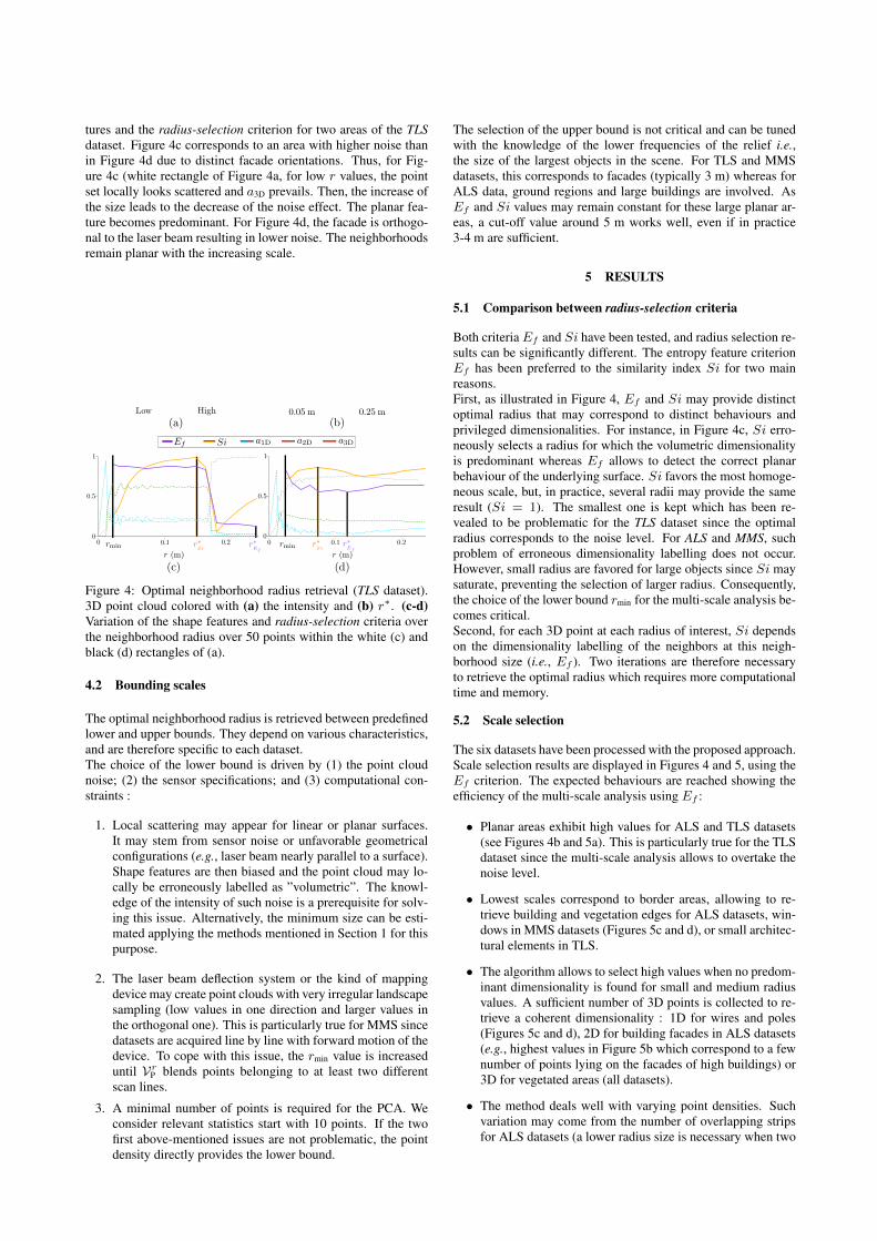
tures and the radius-selection criterion for two areas of the TLSdataset. Figure 4c corresponds to an area with higher noise thanin Figure 4d due to distinct facade orientations. Thus, for Fig-ure 4c (white rectangle of Figure 4a, for low r values, the pointset locally looks scattered and a3D prevails. Then, the increase ofthe size leads to the decrease of the noise effect. The planar fea-ture becomes predominant. For Figure 4d, the facade is orthogo-nal to the laser beam resulting in lower noise. The neighborhoodsremain planar with the increasing scale.

Figure 4: Optimal neighborhood radius retrieval (TLS dataset).3D point cloud colored with (a) the intensity and (b) r∗. (c-d)Variation of the shape features and radius-selection criteria overthe neighborhood radius over 50 points within the white (c) andblack (d) rectangles of (a).

4.2 Bounding scales

The optimal neighborhood radius is retrieved between predefinedlower and upper bounds. They depend on various characteristics,and are therefore specific to each dataset.The choice of the lower bound is driven by (1) the point cloudnoise; (2) the sensor specifications; and (3) computational con-straints :

1. Local scattering may appear for linear or planar surfaces.It may stem from sensor noise or unfavorable geometricalconfigurations (e.g., laser beam nearly parallel to a surface).Shape features are then biased and the point cloud may lo-cally be erroneously labelled as ”volumetric”. The knowl-edge of the intensity of such noise is a prerequisite for solv-ing this issue. Alternatively, the minimum size can be esti-mated applying the methods mentioned in Section 1 for thispurpose.

2. The laser beam deflection system or the kind of mappingdevice may create point clouds with very irregular landscapesampling (low values in one direction and larger values inthe orthogonal one). This is particularly true for MMS sincedatasets are acquired line by line with forward motion of thedevice. To cope with this issue, the rmin value is increaseduntil Vr

P blends points belonging to at least two differentscan lines.

3. A minimal number of points is required for the PCA. Weconsider relevant statistics start with 10 points. If the twofirst above-mentioned issues are not problematic, the pointdensity directly provides the lower bound.

The selection of the upper bound is not critical and can be tunedwith the knowledge of the lower frequencies of the relief i.e.,the size of the largest objects in the scene. For TLS and MMSdatasets, this corresponds to facades (typically 3 m) whereas forALS data, ground regions and large buildings are involved. AsEf and Si values may remain constant for these large planar ar-eas, a cut-off value around 5 m works well, even if in practice3-4 m are sufficient.

5 RESULTS

5.1 Comparison between radius-selection criteria

Both criteriaEf and Si have been tested, and radius selection re-sults can be significantly different. The entropy feature criterionEf has been preferred to the similarity index Si for two mainreasons.First, as illustrated in Figure 4, Ef and Si may provide distinctoptimal radius that may correspond to distinct behaviours andprivileged dimensionalities. For instance, in Figure 4c, Si erro-neously selects a radius for which the volumetric dimensionalityis predominant whereas Ef allows to detect the correct planarbehaviour of the underlying surface. Si favors the most homoge-neous scale, but, in practice, several radii may provide the sameresult (Si = 1). The smallest one is kept which has been re-vealed to be problematic for the TLS dataset since the optimalradius corresponds to the noise level. For ALS and MMS, suchproblem of erroneous dimensionality labelling does not occur.However, small radius are favored for large objects since Si maysaturate, preventing the selection of larger radius. Consequently,the choice of the lower bound rmin for the multi-scale analysis be-comes critical.Second, for each 3D point at each radius of interest, Si dependson the dimensionality labelling of the neighbors at this neigh-borhood size (i.e., Ef ). Two iterations are therefore necessaryto retrieve the optimal radius which requires more computationaltime and memory.

5.2 Scale selection

The six datasets have been processed with the proposed approach.Scale selection results are displayed in Figures 4 and 5, using theEf criterion. The expected behaviours are reached showing theefficiency of the multi-scale analysis using Ef :

• Planar areas exhibit high values for ALS and TLS datasets(see Figures 4b and 5a). This is particularly true for the TLSdataset since the multi-scale analysis allows to overtake thenoise level.

• Lowest scales correspond to border areas, allowing to re-trieve building and vegetation edges for ALS datasets, win-dows in MMS datasets (Figures 5c and d), or small architec-tural elements in TLS.

• The algorithm allows to select high values when no predom-inant dimensionality is found for small and medium radiusvalues. A sufficient number of 3D points is collected to re-trieve a coherent dimensionality : 1D for wires and poles(Figures 5c and d), 2D for building facades in ALS datasets(e.g., highest values in Figure 5b which correspond to a fewnumber of points lying on the facades of high buildings) or3D for vegetated areas (all datasets).

• The method deals well with varying point densities. Suchvariation may come from the number of overlapping stripsfor ALS datasets (a lower radius size is necessary when two

Figure 5: Radius selection (r) and dimensionality labelling for (a) ALSG, (b) ALSF , (c) MMSU , and (d) MMSF datasets.

overlapping strips exist for an area of interest, see Fig-ure 5b), from occlusions or from the fluctuating incidenceangle of the laser beam on the surfaces for TLS or MMSdatasets (Figure 5d).

Figure 6: dimensionality labelling statistics for two datasetsavailable with ground truth. (a) ALSG dataset: the five mainclasses have been conserved. (b) MMSU dataset: the 59 classeshave been condensed into four classes according to their shape(1D: wires, poles, trunks etc. – 2D: wall, door, facade etc. – 3D:foliage, grass etc. – Clutter: objects without specific shapes). Thenumber of points for each class is indicated inside brackets.

The effectiveness of the scale selection process can be assessedby retrieving the predominant dimensionality that has been re-trieved (1D, 2D or 3D ?) for various objects of interest. Severalexamples are presented in Figure 5, and comparisons with manu-ally labelled ALS and MMS data have been performed (cf. Fig-ure 6). For both datasets, planar objects are correctly retrieved,with few errors corresponding to building edges or small urbanitems, especially for ALS data. Besides, objects with one privi-leged dimension such as poles, wires or trunks are mainly labelledas 1D (MMSU dataset, in Figure 6b). However, since these ob-jects are in fact cylindrical with a small width (e.g., trunks or traf-fic lights), they may look planar or volumetric for medium-sizedneighborhoods. Conversely, volumetric objects such as trees maylocally look planar. This happens for large objects low point den-sities or when no multiple scatterings are found with vegetatedareas. Such phenomena is limited for genuine 3D acquisitions(TLS or MMS datasets), whereas it is clearly enhanced for 2.5D

data such as for the ALSR data (Figure 6a). High vegetation ar-eas are principally labelled as planar, which is due to the densecanopy cover. Nevertheless, as displayed in Figure 5a, such ef-fect almost disappears when 3D points are acquired within treecanopies.

5.3 Comparisons with constant neighborhood size

The adaptive size strategy allows to retrieve a correct number ofpoints to estimate the local dimensionality of the point set. Suchstrategy may be compared with the results achieved with neigh-borhoods of fixed size for a whole dataset.Firstly, the three shape features are computed with both strategiesfor four classes of interest of the ALSR dataset (Figure 7). Onecan see that the planar behaviour of ground and building points isimproved with the adaptive size. Besides, for vegetated areas, thevolumetric behaviour is slightly enhanced, however this happensin conjunction with an increase of the planar behaviour (densecanopies).

Figure 7: Improvements in shape feature computation using anoptimal neighborhood radius per point. adD and a∗dD are the shapefeature for dimensionality d, computed with neighborhoods ofconstant size and adaptive size, respectively. The constant neigh-borhood size corresponds to the 30 nearest neighbors of eachpoint.

Secondly, in addition to improved shape features, Figure 8 showsthat the privileged dimensionality is also better retrieved with the

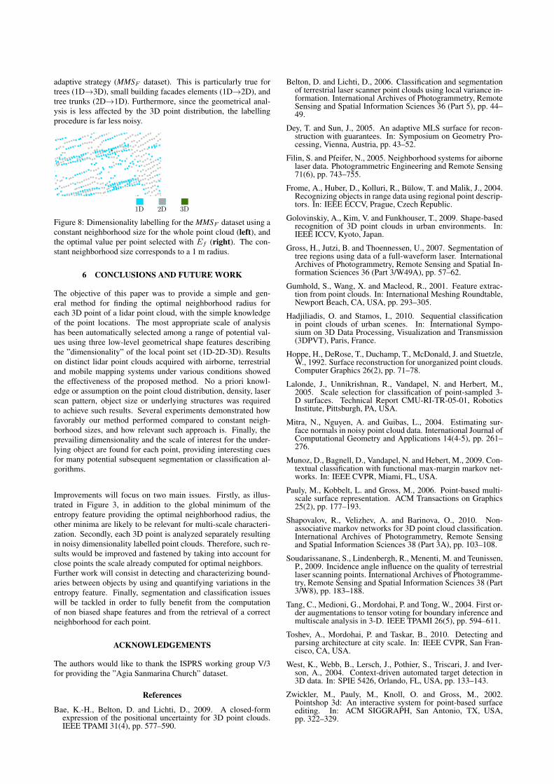
adaptive strategy (MMSF dataset). This is particularly true fortrees (1D→3D), small building facades elements (1D→2D), andtree trunks (2D→1D). Furthermore, since the geometrical anal-ysis is less affected by the 3D point distribution, the labellingprocedure is far less noisy.

Figure 8: Dimensionality labelling for the MMSF dataset using aconstant neighborhood size for the whole point cloud (left), andthe optimal value per point selected with Ef (right). The con-stant neighborhood size corresponds to a 1 m radius.

6 CONCLUSIONS AND FUTURE WORK

The objective of this paper was to provide a simple and gen-eral method for finding the optimal neighborhood radius foreach 3D point of a lidar point cloud, with the simple knowledgeof the point locations. The most appropriate scale of analysishas been automatically selected among a range of potential val-ues using three low-level geometrical shape features describingthe ”dimensionality” of the local point set (1D-2D-3D). Resultson distinct lidar point clouds acquired with airborne, terrestrialand mobile mapping systems under various conditions showedthe effectiveness of the proposed method. No a priori knowl-edge or assumption on the point cloud distribution, density, laserscan pattern, object size or underlying structures was requiredto achieve such results. Several experiments demonstrated howfavorably our method performed compared to constant neigh-borhood sizes, and how relevant such approach is. Finally, theprevailing dimensionality and the scale of interest for the under-lying object are found for each point, providing interesting cuesfor many potential subsequent segmentation or classification al-gorithms.

Improvements will focus on two main issues. Firstly, as illus-trated in Figure 3, in addition to the global minimum of theentropy feature providing the optimal neighborhood radius, theother minima are likely to be relevant for multi-scale characteri-zation. Secondly, each 3D point is analyzed separately resultingin noisy dimensionality labelled point clouds. Therefore, such re-sults would be improved and fastened by taking into account forclose points the scale already computed for optimal neighbors.Further work will consist in detecting and characterizing bound-aries between objects by using and quantifying variations in theentropy feature. Finally, segmentation and classification issueswill be tackled in order to fully benefit from the computationof non biased shape features and from the retrieval of a correctneighborhood for each point.

ACKNOWLEDGEMENTS

The authors would like to thank the ISPRS working group V/3for providing the ”Agia Sanmarina Church” dataset.

References

Bae, K.-H., Belton, D. and Lichti, D., 2009. A closed-formexpression of the positional uncertainty for 3D point clouds.IEEE TPAMI 31(4), pp. 577–590.

Belton, D. and Lichti, D., 2006. Classification and segmentationof terrestrial laser scanner point clouds using local variance in-formation. International Archives of Photogrammetry, RemoteSensing and Spatial Information Sciences 36 (Part 5), pp. 44–49.

Dey, T. and Sun, J., 2005. An adaptive MLS surface for recon-struction with guarantees. In: Symposium on Geometry Pro-cessing, Vienna, Austria, pp. 43–52.

Filin, S. and Pfeifer, N., 2005. Neighborhood systems for aibornelaser data. Photogrammetric Engineering and Remote Sensing71(6), pp. 743–755.

Frome, A., Huber, D., Kolluri, R., Bulow, T. and Malik, J., 2004.Recognizing objects in range data using regional point descrip-tors. In: IEEE ECCV, Prague, Czech Republic.

Golovinskiy, A., Kim, V. and Funkhouser, T., 2009. Shape-basedrecognition of 3D point clouds in urban environments. In:IEEE ICCV, Kyoto, Japan.

Gross, H., Jutzi, B. and Thoennessen, U., 2007. Segmentation oftree regions using data of a full-waveform laser. InternationalArchives of Photogrammetry, Remote Sensing and Spatial In-formation Sciences 36 (Part 3/W49A), pp. 57–62.

Gumhold, S., Wang, X. and Macleod, R., 2001. Feature extrac-tion from point clouds. In: International Meshing Roundtable,Newport Beach, CA, USA, pp. 293–305.

Hadjiliadis, O. and Stamos, I., 2010. Sequential classificationin point clouds of urban scenes. In: International Sympo-sium on 3D Data Processing, Visualization and Transmission(3DPVT), Paris, France.

Hoppe, H., DeRose, T., Duchamp, T., McDonald, J. and Stuetzle,W., 1992. Surface reconstruction for unorganized point clouds.Computer Graphics 26(2), pp. 71–78.

Lalonde, J., Unnikrishnan, R., Vandapel, N. and Herbert, M.,2005. Scale selection for classification of point-sampled 3-D surfaces. Technical Report CMU-RI-TR-05-01, RoboticsInstitute, Pittsburgh, PA, USA.

Mitra, N., Nguyen, A. and Guibas, L., 2004. Estimating sur-face normals in noisy point cloud data. International Journal ofComputational Geometry and Applications 14(4-5), pp. 261–276.

Munoz, D., Bagnell, D., Vandapel, N. and Hebert, M., 2009. Con-textual classification with functional max-margin markov net-works. In: IEEE CVPR, Miami, FL, USA.

Pauly, M., Kobbelt, L. and Gross, M., 2006. Point-based multi-scale surface representation. ACM Transactions on Graphics25(2), pp. 177–193.

Shapovalov, R., Velizhev, A. and Barinova, O., 2010. Non-associative markov networks for 3D point cloud classification.International Archives of Photogrammetry, Remote Sensingand Spatial Information Sciences 38 (Part 3A), pp. 103–108.

Soudarissanane, S., Lindenbergh, R., Menenti, M. and Teunissen,P., 2009. Incidence angle influence on the quality of terrestriallaser scanning points. International Archives of Photogramme-try, Remote Sensing and Spatial Information Sciences 38 (Part3/W8), pp. 183–188.

Tang, C., Medioni, G., Mordohai, P. and Tong, W., 2004. First or-der augmentations to tensor voting for boundary inference andmultiscale analysis in 3-D. IEEE TPAMI 26(5), pp. 594–611.

Toshev, A., Mordohai, P. and Taskar, B., 2010. Detecting andparsing architecture at city scale. In: IEEE CVPR, San Fran-cisco, CA, USA.

West, K., Webb, B., Lersch, J., Pothier, S., Triscari, J. and Iver-son, A., 2004. Context-driven automated target detection in3D data. In: SPIE 5426, Orlando, FL, USA, pp. 133–143.

Zwickler, M., Pauly, M., Knoll, O. and Gross, M., 2002.Pointshop 3d: An interactive system for point-based surfaceediting. In: ACM SIGGRAPH, San Antonio, TX, USA,pp. 322–329.