1 of 36

Digital field tape format standards — SEG-D1 SEG Subcommittee on Digital Tape Formats2

The evolving nature of the seismic data acquisition requires a corresponding change in the recording techniques of these data. Several recording formats have been defined in the past to accommodate the previous changes in instrumentation. They were: SEG's A, B, C, and Y. The following described format includes the best features from these previous formats plus additional characteristics.

By using this new tape format, the data may be multiplexed or demultiplexed, the multiplexed records may be gapped or gapless. The data values are recorded in one of six methods; they are: eight bits or sixteen bits using a quaternary or hexadecimal exponent, twenty bits with a binary exponent, or thirty-two bits with a hexadecimal exponent. The diversity of information to be recorded required a record header that would self-define all the recorded data. Each seismic channel can be individually identified as to its start-stop time, sampling interval, filtering and type of data information recorded.

Included are examples of the defined parameters, example calculations, a glossary, and descriptors for the abbreviations used.

1 © 1975 Society of Exploration Geophysicist, All rights reserved. 2 D.A. Cavers (Chairman), Gulf Research and Development, Box 36506, Houston, TX 77036; P.E. Carroll, Texas Instruments, P.O. Box 1444, M.S. 6i7, Houston, TX 77001; E.P. Meiners, Chevron Geophysical, Box 36487, Houston, TX 77036; C.W. Racer, Chevron Geophysical, 8114 Pella, Houston, TX 77036; L.E. Siems, Litton Resources, 3930 Westholme Drive, Houston, TX 77063; M.G. Sojourner, Input/Output, 8009 Harwin Drive, Houston, TX 77036; J.L. Twombly, GUS Manufacturing, 10486 Dauwood, E1 Paso, TX 79925; J.A. Weigand, Texaco Inc., 4800 Foumace Place E302, Bellaire, TX 77401.

INTRODUCTION

During the past 12 years, a number of recommendations have been published describing proposed tape format standards for both seismic field recording and for seismic trade data (ANSI, 1973a, b, 1976). Many of today's needs, however, were not anticipated in these designs. For example, past formats do not provide for submillisecond sampling intervals, are limited in range and slope of filters, arc restricted in the number of recording channels, and make no provisions for either multiple sampling intervals or dynamic changes in parameters such as filters or sampling intervals. This proposal's objective is to overcome these restrictions while at the same time maintaining some compatibility with the presently used formats.

We propose a family of formats all with the same header structure, encompassing both multiplexed and demultiplexcd data, with 1, 2, 2½, and 4 byte data words. It is not intended to replace SEG's A, B, C, or Y standard formats. (Northwood et al, 1967; Meiners et al, 1972; Barry et al, 1975). The family is given the designation SEG-D followed by a code number defining the type of data word, and the designation "multiplexed" or

"demultiplexed." The code numbers recommended are listed in Appendix A under Bytes 3 and 4 of the general header.

GENERAL FORMAT

The following requirements have been incorporated:

(1) The nine track one-half inch tape is retained, but extension to 6250 BPI is permitted as long as it is compatible with the ANSI standard (ANSI 1973a, b, 1976).

(2) Both multiplexed and demultiplexed field tape formats are represented.

(3) Various word length formats are provided to allow trade-offs to be made when recording large numbers of channels at short sampling intervals.

(4) Multiple sets of data channels can be recorded, each operating at a different sampling interval, or each having other parameter differences (e.g., filters) during the record. The parameters can be constant throughout the record, or can be dynamically switched at some predetermined time.

This document has been converted from the original publication: Barry, K. M., Cavers, D. A. and Kneale, C. W., 1975, Report on recommended standards for digital tape formats: Geophysics, 40, no. 02, 344-352.

2 of 36

(5) The format is self-defining. Information in the header specifies the length of the header and the length of the data record.

(6) A one's complement number system is selected for the fractional part in all binary and quaternary exponent data recording methods. A sign and magnitude number system is selected for the fractional part of all hexadecimal exponent data recording methods.

(7) A unique four byte start of scan code is used. Status bits are provided to indicate dynamic changes starting with this scan.

(8) Submillisecond timing words are incorporated to allow shorter sampling interval systems to have a unique timing word in each scan.

(9) One start of scan code followed by a timing word is utilized in all multiplexed formats in order to facilitate software and hardware synchronization.

(10) Provisions are made for recording the instrument sample skew in the header. (This does not include cable propagation delay which must be established by the user.)

FORMAT OVERVIEW

The overall tape layout is as follows:

Leader BOT Seismic record file 1 EOF Seismic record file 2 EOF

• • •

Seismic record file n EOF EOF EOT Trailer

As shown in Figure 1, each seismic record consists of

a file of two or more blocks. The first block contains the record headers. Following the header block will be one or more blocks of multiplexed data (Figure 2) or of demultiplexed data (Figure 3). Seismic records are separated by one end. of file mark (EOF). Two EOF marks indicate that there are no more seismic records on the tape.

HEADER BLOCK — FUNCTIONAL DESCRIPTION

The record header block is a single block of infor-mation separated from the data by a standard inter-block gap. The record header block is composed of a general header, one or more scan type headers and, optionally, the extended and external headers (Figure 1). All header information is packed BCD unless otherwise specified, with bit positions 0-3 being the most significant digit. Appendix A has a detailed listing of the information contained in the general and scan type headers. General header (required)

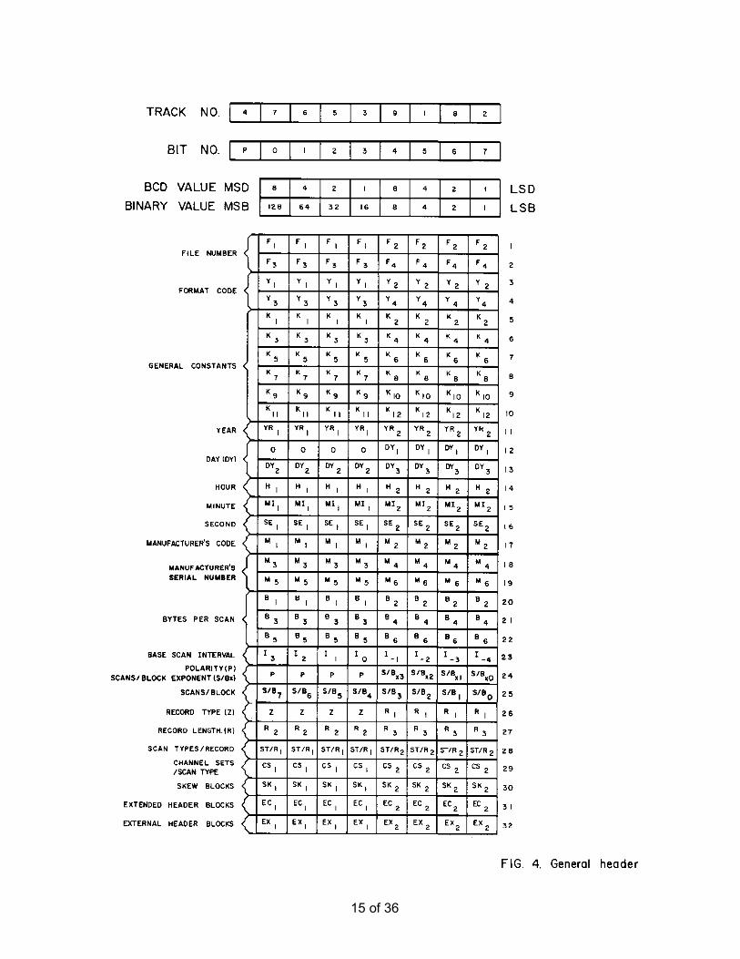
The general header is 32 bytes long and contains information similar to SEG A, B, and C headers (Figure 4). Abbreviations (Appendix D) are as close as possible to those used in previous formats. Scan type header (required)

The scan type header is new. It is used to describe the information of the recorded channels [filters, sampling intervals, sample skew, etc. (Figure 6)]. The scan type header is composed of one or more channel set descriptors followed by skew information. The channel set descriptors must appear in the same order as their respective channel sets will appear within a base scan interval. A channel set, which is part of a scan type, is defined as a group of channels all recorded with identical recording parameters. One or more channel sets can be recorded concurrently within one scan type. In addition, there can be multiple scan types to permit dynamic scan type changes during the record (e.g., 12 channels at ½ msec switched at about 1 sec to 48 channels at 2 msec). Where there are dynamic changes, scan type header 1 describes the first part of the record, scan type header 2 the second part, etc. Within the scan type header, each channel set descriptor is composed of a 32 byte field (Figure 5), and up to 99 channel set descriptors may be present. In addition, up to 99 scan type headers may be utilized in a record.

Following the channel set descriptors of a scan type are a number of 32 byte fields (SK, specified in Byte 30 of the general header) that specify sample skew. Sample skew (SS) is recorded in a single byte for each sample of each subscan of each channel set, in the same order as the samples are recorded in the scan. Each byte represents a fractional part of the base scan interval (Byte 23 of the general header). The resolution is 1/256 of this interval. For instance, if the base scan interval is 2 msec, the least significant bit in the sample skew byte is 1/256 of 2 msec or 7.8125 µsec. The reference point for the skew is the timing word (T) such that the timing word represents zero skew. The actual time the sample was taken is obtained

3 of 36

by adding the timing word (T) to the product of the sample skew (SS) and the base scan interval (I). (Actual time = T + SS x I.)

The following is a list of ground roles for the scan type header:

(1) The order in which channel sets are described in the header will be the same as the order in which the data are recorded for each channel set. (See multiplexed data example 6.)

(2) In a scan type header containing multiple channel set descriptors with different sampling intervals, each channel set descriptor will appear only once in each scan type header. Within the data block, however, shorter sampling interval data are recorded more frequently (i.e., within a base scan interval, channel sets of a shorter sampling interval will appear as multiple subscans). The number of subscans of a channel set is equal to the quotient of the base scan interval divided by the channel set sampling interval [see Byte 12 of the descriptor for this channel set (Figure 5)].

(3) In the case of multiple scan type records, such as the dynamically switched sampling interval case, each scan type will contain the same number of channel sets. Any unused channel sets needed in a scan type must be so indicated by setting Bytes 9 and 10 (channels per channel set) to zero in the channel set descriptor (Appendix A).

(4) In multiple scan type records, the number of bytes per base scan interval must remain a constant for all scan types recorded.

(5) The data recording method is not permitted to change on a reel of tape. However, multiplexed and demultiplexed data may appear on the same reel. For example, one or more multiplexed or demultiplexcd records may be recorded on tape followed by a multiplexed or demultiplexed stacked record of the same data with the same word length and data recording method.

(6) Although not essential, it is suggested that the channel set order within a scan type be: auxiliary channels, long sampling interval channels, short sampling interval channels. All channel sets of the same sampling interval should be contiguous (see Example 4).

Extended header (optional)

The extended header provides additional areas to be used by equipment manufacturers to interface directly with their equipment. An example of this would be a vertical stacking unit used in conjunction with the data acquisition system (e.g., records per stack, records rejected in stack, type of stack, etc.). Since the nature of

this data will depend heavily on the equipment and processes being applied, it will be the responsibility of the equipment manufacturer to establish a format and document this area. Byte 31 of the general header contains the number of 32 byte fields in the extended header. External header (optional)

The external header provides a means of recording special user desired information in the header block. Some examples of this are roll box information, crew data, survey information, and a multiplicity of marine parameters. This data format will be defined and documented by the end user. The means of putting this information into the header has usually been provided by the equipment manufacturer. Byte 32 of the general header contains the number of 32 byte fields in the external header.

DATA BODY Multiplexed

The multiplexed data may be gapped or gapless. A gapless multiplexed data block (Figure 2) is one continuous block of data separated from the header block by an interblock gap, and divided into an integral number of scans as defined in the header. If the multiplexed data body is gapped, each block must begin with a start-of-scan and must contain an integral number of scans. Bytes 24 and 25 of the general header indicate the number of scans in a block. Zero indicates gapless data.

In each scan the first eight bytes are dedicated to the start-of-scan code and timing word as shown in Figure 8. The sync code and timing word provide a means of recovering data that might otherwise be lost, and allow various checks to be made on the integrity of the data while it is being read during processing.

The 8 byte start-of-scan code and timing word over-head must be considered (counted) when computing the number of bytes per scan. The 8 byte start-of-scan and timing word format will remain the same in each of the different data recording methods. The start-of-scan code in each of the data recording methods described here must be maintained as a unique 4 byte code; therefore, there will be certain restrictions on the data in each of the different data recording methods which are covered in the individual format descriptions. (See general header Bytes 3 and 4.)

The 4 byte (start of scan) code as shown in Figure 8 and below is composed as follows: The first three bytes are all one's, and Bits 6 and 7 of Byte 4 must be a zero and a one, respectively, to guarantee uniqueness of the start of scan. The remaining bits (0-5) of Byte 4 are

4 of 36

undefined (x) or are used as follows:

Start of scan Bit 0 1 2 3 4 5 6 7 Byte 1 1 1 1 1 1 1 1 1 Byte 2 1 1 1 1 1 1 1 1 Byte 3 1 1 1 1 1 1 1 1 Byte 4 x TWI ITB DP x x 0 1

TWI. — This bit is included as an integrity check on time break. It changes from a zero to a one at the close of the time break window. Random variations in the time of this change indicate a problem in the fire control system. The presence of a one in the TWI bit of the first start of scan of a record indicates that time break was not detected and recording commenced at the end of the time break window.

ITB. — Intemal time break is recorded as a 1 for the entire record if an abnormal condition is detected in the synchronization of the system timing with the energy source timing. Otherwise it is recorded as a zero.

DP. — The dynamic parameter change bit is recorded as a zero for the first scan of every record and remains a zero throughout the first scan type. It is switched from a zero to a one to indicate the first scan of the second scan type which contains the first data taken after a dynamic parameter change has occurred. It will remain a one throughout the second scan type until another dynamic parameter change occurs, at which time it will be switched to a zero. It is alternately switched at each subsequent scan type. For records without dynamic parameter changes, it is recorded as a zero throughout the record.

The next three bytes (Bytes 5-7 of the scan) are dedicated to a binary timing word as shown in Figure 8 and below. Byte 8 is written as all zeros. The timing word is in milliseconds and has the following bit weight assignments:

Timing word

Bit 0 1 2 3 4 5 6 7 Byte 5 215 214 213 212 211 210 29 28 Byte 6 27 26 25 24 23 22 21 20 Byte 7 2-1 2-2 2-3 2-4 2-5 2-6 2-7 2-8 Byte 8 0 0 0 0 0 0 0 0 The timing word LSB (2-8) is equal to 1/256 msec, and the MSB (215) is equal to 32,768 msec. The timing word for each scan is equal to the elapsed time from zero time to the start of that scan. Timing words of from 0 to 65,535.9961 msec are codable. For longer recordings the timing word may overflow to zero and then continue.

The first scan of data has typically started with timing

word zero. However, this is not a requirement. In a sampling system, it is not always practical to resynchronize the system even though most seismic data acquisition systems have to date. Possible reasons for not wanting to resynchronize could be digital filtering, communication restrictions, etc.

Whether the system is resynchronized or not, the timing word will contain the time from the energy source event to the start of scan of interest. For example, assume the sampling interval is 2 msec, the system does not resynchronize, and the energy source event occurs 1 + 9/256 msec before the next normal start of scan. The timing word values would be: First timing word 0 + 1 + 9/256 msec Second 2 + 1 + 9/256 msec Third 4 + 1 + 9/256 msec Fourth 6 + 1 + 9/256 msec

• • •

One-thousandth timing word

1998 + 1 + 9/256 msec

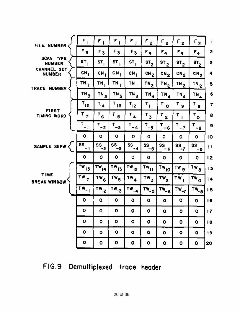
Demultiplexed The demultiplexed data format (Figure 3) is simply an extension of the multiplexed format previously described (Figure 2). In an equivalent system, it would utilize the same header block as its multiplexed counterpart with the exception of the format code in Bytes 3 and 4 and bytes per scan in Bytes 20, 21, and 22 of the general header. The data body portion of the multiplexed format (as shown in Figure 2) is replaced with individual trace blocks (Figure 3) including a trace header (see Figure 9 and below) for all channels in each channel set of each scan type. Each trace block is separated by a standard inter block gap of erased tape and is a sequential set of points from one channel in one channel set. The data recording methods utilized within the trace blocks are de-scribed later in the section titled "Data recording method."

Trace header. — The trace header length is 20 bytes and is an identifier that precedes each channel's data. The trace header and the trace data are recorded as one block of data. A trace is restricted to one channel of data from one channel set of one scan type. All the information in the trace header is taken directly from the general header and scan type header with the exception of the channel number and the time break window end time. File number, scan type, channel set, and channel (or trace) number are recorded in packed BCD.

Bytes 7, 8, and 9 comprise the timing word that would accompany the first sample if these data were written in the multiplexed format. To obtain the exact sample time, the actual sample skew time (Byte 11 multiplied by the base scan interval) must be added to the

5 of 36

time recorded in Bytes 7, 8, and 9. Byte 11 contains sample skew of the first sample of

this trace. This is identical to the first byte of sample skew for this channel in the scan type header. Bytes 13, 14, and 15 are included as an integrity check on time break. They comprise the timing word of the scan in which TWI changed to a one. Thus, it represents the time from time break to the end of the time break window. Random variations in this time indicate a problem in the fire control system. The presence of a value less than the

base scan interval indicates that time break was not detected and recording commenced at the end of the time break window.

DATA RECORDING METHOD To accommodate diverse recording needs, the data

recording utilizes sample sizes of 8, 16, 20, and 32 bits. The data word is a number representation of the sign

Trace header

Bit 0 1 2 3 4 5 6 7

File number Byte 1 F1 F1 F1 F1 F2 F2 F2 F2

Byte 2 F3 F3 F3 F3 F4 F4 F4 F4

Scan type Byte 3 ST1 ST1 ST1 ST1 ST2 ST2 ST2 ST2

Channel set Byte 4 CN1 CN1 CN1 CN1 CN2 CN2 CN2 CN2

Byte 5 TN1 TN1 TN1 TN1 TN2 TN2 TN2 TN2 Channel or

trace number Byte 6 TN3 TN3 TN3 TN3 TN4 TN4 TN4 TN4

Byte 7 T15 T14 T13 T12 T11 T10 T9 T8

Byte 8 T7 T6 T5 T4 T3 T2 T1 T0

Byte 9 T-1 T-2 T-3 T-4 T-5 T-6 T-7 T-8

First timing

word

Byte 10 0 0 0 0 0 0 0 0

Byte 11 SS-1 SS-2 SS-3 SS-4 SS-5 SS-6 SS-7 SS-8 Sample skew

Byte 12 0 0 0 0 0 0 0 0

Byte 13 TW15 TW14 TW13 TW12 TW11 TW10 TW9 TW8

Byte 14 TW7 TW6 TW5 TW4 TW3 TW2 TW1 TW0 Time break

window end Byte 15 TW-1 TW-2 TW-3 TW-4 TW-5 TW-6 TW-7 TW-8

Byte 16 0 0 0 0 0 0 0 0

Byte 17 0 0 0 0 0 0 0 0

Byte 18 0 0 0 0 0 0 0 0

Byte 19 0 0 0 0 0 0 0 0

Byte 20 0 0 0 0 0 0 0 0

6 of 36

and magnitude of the instantaneous voltage presented to the system. It is not an indication of how the hardware gain system functions. The output of stepped gain systems may be represented as a binary mantissa and a binary exponent of base 2, 4, or 16 (binary, quaternary, or hexadecimal system).

Following are descriptions of each of the data

recording methods permitted. The same number system is to be used on all samples in a record, including auxiliary and all other types of channels. All recording methods are valid for multiplexed and demultiplexed records. The 2½ byte binary demultiplexed method uses the LSB whereas the comparable multiplexed method does not (in order to preserve the uniqueness of the start of scan code).

1 byte quaternary exponent data recording method

The following illustrates the 8 bit word and the corresponding bit weights:

Bit 0 1 2 3 4 5 6 7 Byte 1 S C2 C1 C0 Q-1 Q-2 Q-3 Q-4

S = sign bit. — (One = negative number). C = quaternary exponent. — This is a three bit positive binary exponent of 4 written as 4CCC where CCC can assume values

from 0-7. Q1-4-fraction. — This is a 4 bit one's complement binary fraction. The radix point is to the left of the most significant bit (Q-1)

with the MSB being defined as 2-1. The fraction can have values from - 1 + 2-4 to 1 - 2-4. In order to guarantee the uniqueness of the start of scan, negative zero is invalid and must be convened to positive zero.

Input signal = S.QQQQ x 4CCC x 2MP millivolts where 2MP is the value required to descale the data sample to the recording system input level. MP is defined in Byte 8 of each channel set descriptor in the scan type header.

2 byte quaternary exponent data recording method

The following illustrated the 16-bit word and the corresponding bit weights:

Bit 0 1 2 3 4 5 6 7 Byte 1 S C2 C1 C0 Q-1 Q-2 Q-3 Q-4 Byte 2 Q-5 Q-6 Q-7 Q-8 Q-9 Q-10 Q-11 Q-12

S = sign bit. — (One = negative number). C = quaternary exponent. — This is a three bit positive binary exponent of 4 written as 4CCC where CCC can assume values

from 0-7. Q1-12 — fraction. — This is a 12 bit one's complement binary fraction. The radix point is to the left of the most significant bit

(Q-1) with the MSB being defined as 2-1. The fraction can have values from –1 + 2-12 to 1 - 2-12. In order to guarantee the uniqueness of the start of scan, negative zero is invalid and must be convened to positive zero.

Input signal = S.QQQQ,QQQQ,QQQQ x 4CCC x 2MP millivolts where 2MP is the value required to de-scale the data sample to the recording system input level. MP is defined in Byte 8 of each channel set descriptor in the scan type header.

2½ byte binary exponent data recording method —multiplexed

The following illustrates the 20-bit word and the corresponding bit weights:

Bit 0 1 2 3 4 5 6 7 Byte 1 C3 C2 C1 C0 C3 C2 C1 C0 Byte 2 C3 C2 C1 C0 C3 C2 C1 C0

Exponent for channels 1 thru 43

Byte 3 S Q-1 Q-2 Q-3 Q-4 Q-5 Q-6 Q-7 Channel 1

3 In the multiplexed format, Bytes 1 and 2 contain the exponents for the following four channels of the scan. The

7 of 36

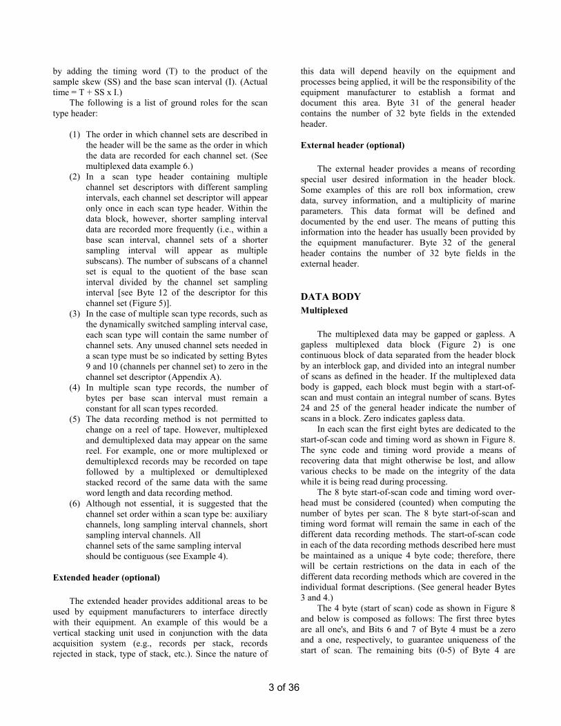
Byte 4 Q-8 Q-9 Q-10 Q-11 Q-12 Q-13 Q-14 0 Byte 5 S Q-1 Q-2 Q-3 Q-4 Q-5 Q-6 Q-7 Byte 6 Q-8 Q-9 Q-10 Q-11 Q-12 Q-13 Q-14 0

Channel 2

Byte 7 S Q-1 Q-2 Q-3 Q-4 Q-5 Q-6 Q-7 Byte 8 Q-8 Q-9 Q-10 Q-11 Q-12 Q-13 Q-14 0

Channel 3

Byte 9 S Q-1 Q-2 Q-3 Q-4 Q-5 Q-6 Q-7 Byte 10 Q-8 Q-9 Q-10 Q-11 Q-12 Q-13 Q-14 0

Channel 4

S = sign bit. — (One = negative number). C = binary exponents. — This is a 4 bit positive binary exponent of 2 written as 2CCCC where CCCC can assume values of 0-

15. The four exponents are in channel number order for the four channels starting with channel one in bits 0-3 of Byte 1.

Ql-14-fraction. — This is a 14 bit one's complement binary fraction. The radix point is to the left of the most significant bit (Q-1) with the MSB being defined as 2-1. The sign and fraction can assume values from 1 - 2-14 to –1 + 2-14. Note that bit 7 of the second byte of each sample must be zero in order to guarantee the uniqueness of the start of scan. Negative zero is invalid and must be convened to positive zero.

Input signal = S.QQQQ,QQQQ,QQQQ,QQ x 2CCCC x 2MP millivolts where 2MP is the value required to descale the data word to the recording system input level. MP is defined in Byte 8 of each of the corresponding channel set descriptors in the scan type header.

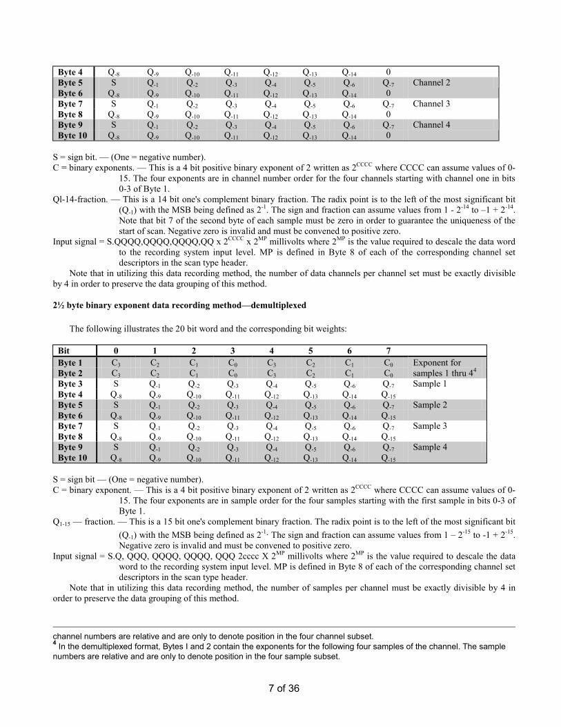
Note that in utilizing this data recording method, the number of data channels per channel set must be exactly divisible by 4 in order to preserve the data grouping of this method. 2½ byte binary exponent data recording method—demultiplexed

The following illustrates the 20 bit word and the corresponding bit weights:

Bit 0 1 2 3 4 5 6 7 Byte 1 C3 C2 C1 C0 C3 C2 C1 C0 Byte 2 C3 C2 C1 C0 C3 C2 C1 C0

Exponent for samples 1 thru 44

Byte 3 S Q-1 Q-2 Q-3 Q-4 Q-5 Q-6 Q-7 Byte 4 Q-8 Q-9 Q-10 Q-11 Q-12 Q-13 Q-14 Q-15

Sample 1

Byte 5 S Q-1 Q-2 Q-3 Q-4 Q-5 Q-6 Q-7 Byte 6 Q-8 Q-9 Q-10 Q-11 Q-12 Q-13 Q-14 Q-15

Sample 2

Byte 7 S Q-1 Q-2 Q-3 Q-4 Q-5 Q-6 Q-7 Byte 8 Q-8 Q-9 Q-10 Q-11 Q-12 Q-13 Q-14 Q-15

Sample 3

Byte 9 S Q-1 Q-2 Q-3 Q-4 Q-5 Q-6 Q-7 Byte 10 Q-8 Q-9 Q-10 Q-11 Q-12 Q-13 Q-14 Q-15

Sample 4

S = sign bit — (One = negative number). C = binary exponent. — This is a 4 bit positive binary exponent of 2 written as 2CCCC where CCCC can assume values of 0-

15. The four exponents are in sample order for the four samples starting with the first sample in bits 0-3 of Byte 1.

Q1-15 — fraction. — This is a 15 bit one's complement binary fraction. The radix point is to the left of the most significant bit (Q-1) with the MSB being defined as 2-1. The sign and fraction can assume values from 1 – 2-15 to -1 + 2-15. Negative zero is invalid and must be convened to positive zero.

Input signal = S.Q, QQQ, QQQQ, QQQQ, QQQ 2cccc X 2MP millivolts where 2MP is the value required to descale the data word to the recording system input level. MP is defined in Byte 8 of each of the corresponding channel set descriptors in the scan type header.

Note that in utilizing this data recording method, the number of samples per channel must be exactly divisible by 4 in order to preserve the data grouping of this method.

channel numbers are relative and are only to denote position in the four channel subset. 4 In the demultiplexed format, Bytes I and 2 contain the exponents for the following four samples of the channel. The sample numbers are relative and are only to denote position in the four sample subset.

8 of 36

1 byte hexadecimal exponent data recording method

The following illustrates the 8-bit word and the corresponding bit weights:

Bit 0 1 2 3 4 5 6 7

Byte 1 S C1 C0 Q-1 Q-2 Q-3 Q-4 Q-5 S = sign bit. — (One - negative number). C = hexadecimal exponent. —This is a two bit positive binary exponent of 16 written as 16CC where CC can assume values

from 0-3. Q1-5 — fraction. —This is a 5 bit positive binary fraction. The radix point is to the left of the most significant bit (Q-1) with

the MSB being defined as 2-1. The sign and fraction can have any value from -1 + 2-5 to 1 – 2-5. In order to guarantee the uniqueness of the start of scan, an all one's representation (sign = negative, exponent = 3, and fraction = 1 – 2-5) is invalid: Thus the full range of values allowed is -( l - 2-4 ) x 163 to + ( l - 2-5 ) x 163.

Input signal = S.QQQQ,Q x 16CC x 2MP millivolts where 2MP is the value required to descale the data sample to the recording system input level. MP is defined in Byte 8 of each channel set descriptor in the scan type header.

2 byte hexadecimal exponent data recording method

The following illustrates the 16-bit word and the corresponding bit weights:

Bit 0 1 2 3 4 5 6 7 Byte l S C1 C0 Q-1 Q-2 Q-3 Q-4 Q-5 Byte 2 Q-6 Q-7 Q-8 Q-9 Q-10 Q-11 Q-12 Q-13

S = sign bit. — (One = negative number). C = hexadecimal exponent. — This is a two bit positive binary exponent of 16 written as 16CC where CC can assume values

from 0-3. Q1-13 — fraction. — This is a 13 bit positive binary fraction. The radix point is to the left of the most significant bit (Q-1 with

the MSB being defined as 2-1 the sign and fraction can have any value from -1 + 2-13 to 1- 2-13. In order to guarantee the uniqueness of the start of scan, an all one's representation (sign = negative, exponent = 3, and fraction = 1 – 2-13) is invalid. Thus the full range of values allowed is -(1 – 2-12) x 163 to + (1 – 2-13) x 163

Input signal = S.QQQQ,QQQQ,QQQQ,Q x 16CC X 2MP millivolts where 2MP is the value required to descale the data sample to the recording system input level. MP is defined in Byte 8 of each channel set descriptor in the scan type header.

4 byte hexadecimal exponent data recording method

The following illustrates the 32-bit word and the corresponding bit weights:

Bit 0 1 2 3 4 5 6 7 Byte 1 S C6 C5 C4 C3 C2 C1 C0 Byte 2 Q-1 Q-2 Q-3 Q-4 Q-5 Q-6 Q-7 Q-8 Byte 3 Q-9 Q-10 Q-11 Q-12 Q-13 Q-14 Q-15 Q-16 Byte 4 Q-17 Q-18 Q-19 Q-20 Q-21 Q-22 Q-23 0

S = sign bit. — (One = negative number). C = excess 64 hexadecimal exponent. — This is a binary exponent of 16. It has been biased by 64 such that it represents

16(CCCCCCC-64) where CCCCCCC can assume values from 0 to 127. Q1-23 — magnitude fraction.—This is a 23 bit positive binary fraction (i.e., the number system is sign and magnitude). The

radix point is to the left of the most significant bit (Q-1) with the MSB being defined as 2-1. The sign and fraction can assume values from 1 – 2-23 to -( 1 + 2-23). It must always be written as a hexadecimal left justified number. If this fraction is zero, the sign and exponent must also be zero (i.e., the entire word is

9 of 36

zero). Note that bit 7 of Byte 4 must be zero in order to guarantee the uniqueness of the start of scan. Input signal = S. QQQQ, QQQQ, QQQQ, QQQQ, QQQQ, QQQ x 16(CCCCCCC-64) x 2MP millivolts where 2MP is the value

required to descale the data sample to the recording system input level. MP is defined in Byte 8 of each channel set descriptor in the scan type header. This data recording method has more than sufficient range to handle the dynamic range of a typical seismic system. Thus, MP may not be needed to account for any scaling and may be recorded as zero.

10 of 36

EXAMPLES

Three sets of examples are given. The header block set illustrates the header lengths for various combinations of scan types and channel sets. The multiplexed data set of examples illustrates the organization of data within scans for an example which includes multiple scan types and multiple channel sets. The demultiplexed data set of examples illustrates the order of trace blocks for most of the examples. Header block

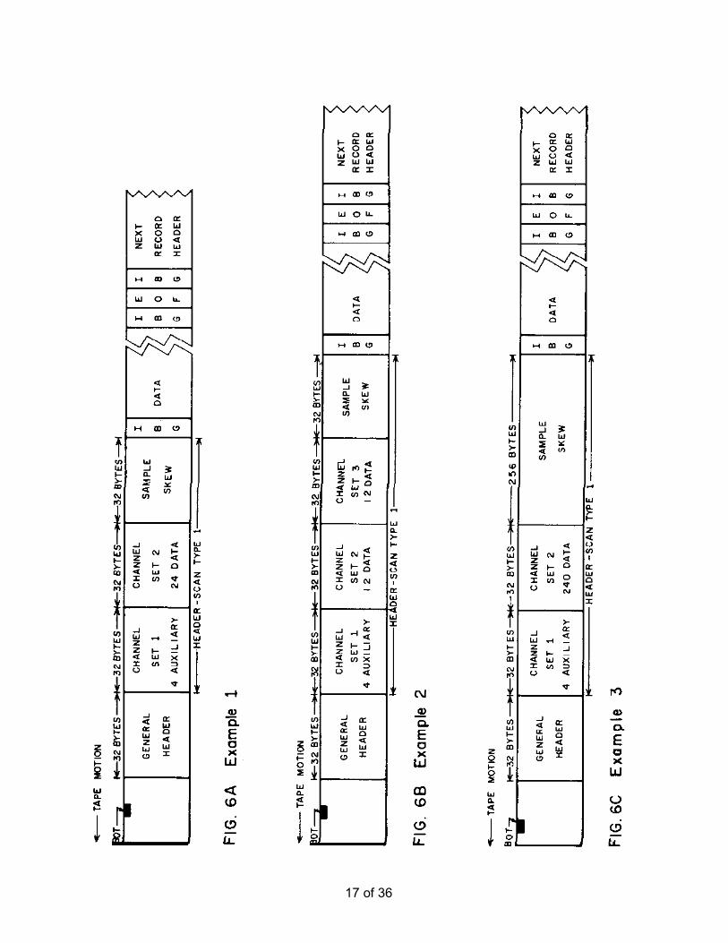
The following examples describe the general and scan type headers required for each case. The optional extended and external headers are not included. Example 1 — Typical 24 channel system (Figure 6A)

4 auxiliary channels at 2-msec sampling intervals 24 seismic channels at 2-msec sampling intervals

This system would contain one scan type header because there are no parameter changes during the record. This one scan type header would contain two channel set descriptors, one for the 4 auxiliary channels and one for the 24 seismic channels. The header block in this case would be as follows, assuming no extensions for the extended and external headers:

32 bytes General header Scan type header 1 32 bytes auxiliary channel set 32 bytes seismic channel set 32 bytes sample skew (28 used) 128 bytes Total header block

Example 2---24 channel system with parameter differences (Figure 6B)

4 auxiliary channels 12 seismic channels with 18-Hz low-cut filters 12 seismic channels with 36-Hz low-cut filters (2-

msec sampling on all channels) This example is similar to the previous one with the exception of needing one additional channel set descriptor, which is required because some of the seismic channels are operating at a different filter setting. The header block in this case would contain one additional 32 byte field.

32 bytes General header Scan type header 1 32 bytes auxiliary channel set 32 bytes seismic channel set (18-Hz low cut) 32 bytes seismic channel set (36-Hz low cut) 32 bytes sample skew (28 used)

160 bytes Total header block Example 3--Large system (Figure 6C)

4 auxiliary channels 240 seismic channels(4 msec sampling on all

channels) The header block in this case will be longer than in Example 1 because it will have additional bytes of sample skew.

32 bytes General header Scan type header 1 32 bytes auxiliary channel set 32 bytes seismic channel set 256 bytes sample skew (244 used) 352 bytes Total header block

Example 4---Dual sampling intervals (Figure 7A)

4 auxiliary channels at 2-msec sampling interval 48 seismic channels at 2-msec sampling interval 12 seismic channels at ½ msec sampling interval

(sampled four times in each scan) In this case there would be three channel set descriptors required to make up the scan type header. The additional channel set descriptor is required to identify the channel set operating at ½ msec.

32 bytes General header Scan type header 1 32 bytes auxiliary channel set 32 bytes seismic channel set at 2 msec 32 bytes seismic channel set at ½ msec 128 bytes sample skew (100 used) 256 bytes Total header block

Example 5---Dynamically switched sampling interval (Figure 7B) Scan type header 1

4 auxiliary channels at 2-msec sampling interval 12 seismic channels at ½ msec sampling interval Scan type header 2 4 auxiliary channels at 2 msec 48 seismic channels at 2 msec This is a switched sampling interval system in which 12 of the channels will be sampled for a portion of the record at a V2-msec interval, then it will switch to 48 seismic channels at a 2-msec interval for the remainder of the record.

This system has a parameter change in mid-record and therefore requires a second scan type header to define it. Its header block would be constructed as follows:

32 bytes General header Scan type header 1

11 of 36

32 bytes 4 auxiliary channels at 2 msec 32 bytes 12 seismic channels at V2 msec 64 bytes Sample Skew (52 used) Scan type header 2 32 bytes 4 auxiliary channels at 2 msec 32 bytes 48 seismic channels at 2 msec 64 bytes Sample skew (52 used) 288 bytes Total header block

Example 6 — Dynamically switched sampling interval (Figure 7C)

This, as in Example 5, is a 2-msec base scan interval system that is dynamically switching sampling interval in mid-record. It starts as a 12 channel, ½ msec sampling interval system and ends as a 48 channel 2 msec sampling interval system with a common filter. The 12 channels in this example, though, are divided into 2 channel sets, with 6 channels utilizing low-cut filters and the remaining 6 without low-cut filters. The header block would be constructed in the following manner:

32 bytes General header Scan type header 1 32 bytes 4 auxiliary channels at 2 msec 32 bytes 6 seismic channels with low-cut

filters at ½ msec 32 bytes 6 seismic channels without

low-cut filters at ½ msec 64 bytes Sample skew (52 used) Scan type header 2 32 bytes 4 auxiliary channels at 2 msec 32 bytes 48 seismic channels at 2 msec 32 bytes 0 channels (dummy) 64 bytes Sample skew (52 used) 352 bytes Total header block

The dummy channel set descriptor is required in scan type header 2 in order to maintain its length equal to that of scan type header I. This preserves easy expandability of the format and its self-defining header length capability (see Appendix E4).

Multiplexed data

Example 6. — The multiplexed data block section of the seismic record is organized in the same order as the scan type headers and channel set descriptors they contain. Within each base scan in scan type 1, all of the data for channel set I are recorded before channel set 2. Likewise, all of the data for channel set 2 are recorded before channel set 3. Because the sampling interval for channel sets 2 and 3 is one-fourth of the base scan interval, each base scan will contain four subscans (a subscan contains one sample from each channel) of channel sets 2 and 3. Furthermore, all four subscans of channel set 2 are recorded before the four subscans of channel set 3. Thus the base scan interval is 2 msec and the data would be recorded in the following order: (I) start of scan and timing word; (2) four auxiliary channels in channel number sequence; (3a) six seismic channels with low-cut filters in channel number sequence; (3b) the second, third, and fourth set of samples of the channels in 3a; (4a) six seismic channels without low-cut filters in channel number sequence; and (4b) the second, third, and fourth sets of samples of the channels in (4a).

The pictorial representation of the multiplexed format of Example 6 as recorded on tape is shown below. Scan type 1 is:

Start of scan and timing word 2 msec base scan

4 Auxiliary channels sampled once each

4 Subscans of 6 seismic channels with low- cut filters sampled at ½ msec

4 Subscans of 6 seismic channels without low- cut filters sampled at ½ msec

Note that this scan is repeated for the required number of scans until the channel set length is satisfied and the sampling interval is changed.

12 of 36

Scan type 2 is:

Start of scan and timing word

4 Auxiliary channels sampled once each at 2 msec

48 Seismic channels sampled once each at 2 msec

Note that this scan type follows the recording of all of scan type 1 and repeats for the required number of scans. Scan types 1 and 2 have the same number of bytes per scan. Demultiplexed data

The following examples are the demultiplexed versions of the previous examples given. Example l. — Typical 24 channel system

The trace blocks in this case would be in the follow-ing order.

4 traces of auxiliary channels 24 traces of seismic data 28 trace blocks total

The channel order above is the same order in which the channel descriptions appear in the scan type header. All other examples of one scan type system follow this pattern. Example 2. — 24 channel system with parameter differences

The trace blocks in this case would be in the following order.

4 traces of auxiliary channels 12 traces of seismic data with 18-Hz low-cut filters

12 traces of seismic data with 36-Hz low-cut filters 28 trace blocks total

Example 3.— Is similar to Example 1, but it has 240 traces of seismic data, resulting in 244 trace blocks total. Example 4. — Dual sampling intervals

The trace blocks in this case would be in the fol-lowing order.

4 traces of auxiliary channels 48 traces of seismic data recorded at a 2 msec

sampling interval 12 traces of seismic data recorded at a ½ msec

sampling interval 64 trace blocks total

Example 5. — Dynamically switched sampling interval

The trace blocks appear in the following order. 4 traces of auxiliary channels, recorded for the length

of scan type 1 12 traces of seismic channels, recorded for the length

of scan type 1 4 traces of auxiliary channels, recorded for the length

of scan type 2 48 traces of seismic channels, recorded for the length

of scan type 2 68 trace blocks total

Example 6. — The following is Example 6 again illustrating in graphical form the order of the trace blocks on tape. Note that even though auxiliary traces 1 to 4 are the same channels in both scan types, the data collected during the time of scan type 1 is recorded separately from those in scan type 2.

Note that there are no traces recorded for channel set 3 of scan type 2. There are 68 trace blocks total. Each new channel set starts with trace number 1.

13 of 36

REFERENCES American National Standards Institute,

1973a, Recorded magnetic tape for information exchange, 800 BPI: ANSI X3.22-1973. 1973b, Recorded magnetic tape for information exchange, 1600 BPI: ANSI X3.39-1973. 1976, Recorded magnetic tape for information exchange, 6250 BPI: ANSI X3.54-1976.

Barry, K.M., Cavers, D.A., and Kneale, C.W., 1975, Recommended standards for digital tape formats:

Geophysics, v. 40, p. 344-352. Dampney, C.N.G., Funkhouser, D., and Alexander, M., 1978,

Structure of the SEG point data exchange and field formats: Geophysics, v. 43, p. 216-227.

Meiners, E.P., Lenz, L.L., Dalby, A.E., and Hornsby, J.M., 1972, Recommended standards for digital tape formats: Geophysics, v. 37, p. 36-44.

Northwood, E.J., Weisinger, R.C., and Bradley, J.J., 1967, Recommended standards for digital tape formats: Geophysics, v. 32, p. 1073-1084.

14 of 36

15 of 36

16 of 36

17 of 36

18 of 36

19 of 36

20 of 36

21 of 36

APPENDIX A HEADER BLOCK PARAMETERS

General header

All values are in packed BCD unless otherwise specified. INDEX ABBREVIATION DESCRIPTION BYTE 1 F1, F2 File number of four 2 F3, F4 digits (0-9999) 3 Y1, Y2 Format code: 4 Y3, Y4 0015 20 bit binary multiplexed 0022 8 bit quaternary multiplexed 0024 16 bit quaternary multiplexed 0042 8 bit hexadecimal multiplexed 0044 16 bit hexadecimal multiplexed 0048 32 bit hexadecimal multiplexed 8015 20 bit binary demultiplexed 8022 8 bit quaternary demultiplexed 8024 16 bit quaternary demultiplexed 8042 8 bit hexadecimal demultiplexed 8044 16 bit hexadecimal &multiplexed 8048 32 bit hexadecimal demultiplexed 0200 Illegal, do not use 0000 Illegal, do not use 5 K1, K2 General constants, 12 digits 6 K3, K4 7 K5, K6 8 K7, K8 9 K9 K10 10 K11, K12 11 YR1, YR2 Last two digits of year (0-99) 12 0, DY1 Julian day 3 digits (1-366) 13 DY2, DY3 14 H1, H2 Hour of day 2 digits (0-23) (Greenwich Mean Time) 1:5 MI1, MI2 Minute of hour 2 digits (0-59) 16 SE1, SE2 Second of minute 2 digits (0-59) 17 M1, M2 Manufacturer's code 2 digits Note: See Appendix B for the current assignments 18 M3, M4 Manufacturer's serial number, 4 digits 19 M5, M6 20 B1, B2 Bytes per scan 6 digits (1-999,999) are utilized in 21 B3, B4 the multiplexed formats to identify the number of 22 B5, B6 bytes (including data, auxiliary, sync, and timing bytes, etc.) required to make up a complete scan. In a demultiplexed record, this field is not used and is recorded as zeros. (See Appendix E2) 23 I3 thru I-4 Base scan interval — This is coded as a binary number with the LSB equal to 1/16 msec. This will allow sampling intervals from 1/16 through 8 msec

22 of 36

INDEX ABBREVIATION DESCRIPTION BYTE in binary steps. Thus, the allowable base scan inter- vals are 1/16, 1/8, 1/4, 1/2, 1, 2, 4, and 8 msec. The base scan interval is always the difference between successive timing words. Each channel used will be sampled one or more times per base scan inter- val. 24 P, Polarity. — These 4 binary bits are measured on the sensors, cables, instrument, and source com- bination and are set into the system manually. The codes are: 0000 Untested 0001 Zero 0010 45 degrees 0011 90 degrees 0100 135 degrees 0101 180 degrees 0110 225 degrees 011l 270 degrees 1000 315 degrees 1001 1010 1011 1100 unassigned 1101 1110 11115 , S/BX7 thru S/BX0 This binary number (range 0 to 15) is an exponent of 2 and is used in conjunction with S/B (Byte 25). 25 S/B7 thru S/B0 This binary number (range 0 to 255) is used in con- junction with S/BX (see Byte 24) to indicate the number of scans in a block. If it is 0, the data body is one continuous block. Otherwise, the data body is composed of multiple blocks, each block con- taining S/B x 2S/BX scans. It is valid only for multiplexed data. 26 Z, Record type Bits 0 1 2 3 0 0 1 0 Test record 0 1 0 0 Parallel channel test 0 1 1 0 Direct channel test 1 0 0 0 Normal record 0 0 0 1 Other , R1 Record length from time zero (in increments of 0.5 27 R2, R3 times 1.024 sec). This value can be set from 00.5 to 99.5 representing times from 0.512 sec. to 101.888 sec. A setting of 00.0 indicates the record length is indeterminate.

5 Details of polarity codes and test methods are listed in the following reference: Thigpen, B. B., Dalby, A. E., Landrum, R., 1975, Special report of the subcommittee on polarity standards' Geophysics, v. 40, p. 694.

23 of 36

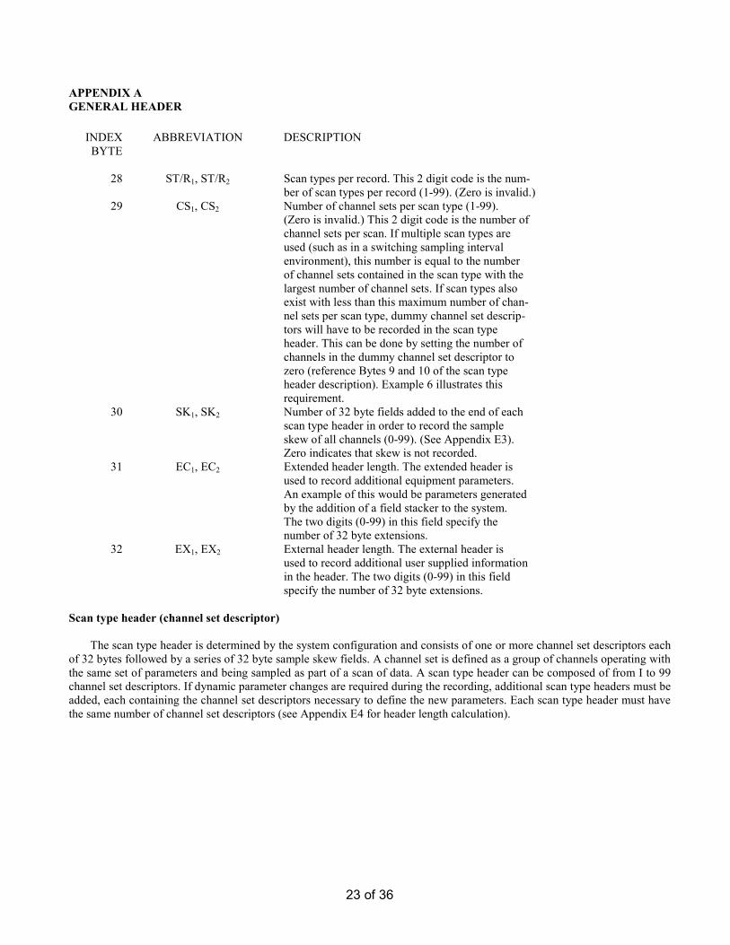
APPENDIX A GENERAL HEADER INDEX ABBREVIATION DESCRIPTION BYTE 28 ST/R1, ST/R2 Scan types per record. This 2 digit code is the num- ber of scan types per record (1-99). (Zero is invalid.) 29 CS1, CS2 Number of channel sets per scan type (1-99). (Zero is invalid.) This 2 digit code is the number of channel sets per scan. If multiple scan types are used (such as in a switching sampling interval environment), this number is equal to the number of channel sets contained in the scan type with the largest number of channel sets. If scan types also exist with less than this maximum number of chan- nel sets per scan type, dummy channel set descrip- tors will have to be recorded in the scan type header. This can be done by setting the number of channels in the dummy channel set descriptor to zero (reference Bytes 9 and 10 of the scan type header description). Example 6 illustrates this requirement. 30 SK1, SK2 Number of 32 byte fields added to the end of each scan type header in order to record the sample skew of all channels (0-99). (See Appendix E3). Zero indicates that skew is not recorded. 31 EC1, EC2 Extended header length. The extended header is used to record additional equipment parameters. An example of this would be parameters generated by the addition of a field stacker to the system. The two digits (0-99) in this field specify the number of 32 byte extensions. 32 EX1, EX2 External header length. The external header is used to record additional user supplied information in the header. The two digits (0-99) in this field specify the number of 32 byte extensions. Scan type header (channel set descriptor)

The scan type header is determined by the system configuration and consists of one or more channel set descriptors each of 32 bytes followed by a series of 32 byte sample skew fields. A channel set is defined as a group of channels operating with the same set of parameters and being sampled as part of a scan of data. A scan type header can be composed of from I to 99 channel set descriptors. If dynamic parameter changes are required during the recording, additional scan type headers must be added, each containing the channel set descriptors necessary to define the new parameters. Each scan type header must have the same number of channel set descriptors (see Appendix E4 for header length calculation).

24 of 36

APPENDIX A CHANNEL SET DESCRIPTOR INDEX ABBREVIATION DESCRIPTION BYTE 1 ST1, ST2 These two digits (1-99) identify the number of the scan type header to be described by the subsequent bytes. The first scan type header is I and the last scan type header number is the same value as Byte 28 (ST/R) of the general header. If a scan type header contains more than one channel set descrip- tor, the scan type header number will be repeated in each of its channel set descriptors. If the sys- tem does not have dynamic parameter changes during the record, such as switched sampling inter- vals, there will only be one scan type header required. 2 CN1, CN2 These two digits (1-99) identify the channel set to be described in the next 30 bytes within this scan type header. The first channel set is "1" and the last channel set number is the same number as Byte 29 (CS) of the general header. If the scan actually contains fewer channel sets than CS, then dummy channel set descriptors are included as specified in Byte 29 of general header. 3 TF16 thru TF9 Channel set starting time. This is a binary number 4 TF8 thru TF1 where TF1 = 21 msec (2-msec increments). This number identifies the timing word of the first scan of data in this channel set. In a single scan type record, this would typically be recorded as a zero (an exception might be deep water recording). In multiple scan type records, this number represents the starting time, in milliseconds, of the channel set. Start times from 0 to 131,070 msec (in 2-msec increments) can be recorded. 5 TEl6 thru TE9 Channel set end time. This is a binary number 6 TE8 thru TE1 where TE1 = 21 milliseconds (2 millisecond incre- ments). These two bytes represent the record end time of the channel set in milliseconds. In a multi- plexed record, all channels of a channel set must be of the same length. TE may be used in a de- multiplexed record to allow the termination of a particular channel set shorter than other channel sets within its scan type. In a single scan type record, Bytes 5 and 6 would be the length of the record. End times up to 131,070 msec (in 2-msec increments) can be recorded. 7 0,0 8 MPS, MP4 thru This sign magnitude binary number is the ex- MP-2 ponent of the base 2 multiplier to be used to descale the data on tape to obtain input voltage in milli- volts. The radix point is between MP0 and MP-1. This multiplier has a range of 231.75 to 2-31.75. (See Appendix E7.) 9 C/S1, C/S2 This is the number of channels in this channel set. 10 C/S3, C/S4 It can assume a number from 0-9999.

25 of 36

INDEX ABBREVIATION DESCRIPTION BYTE 11 C1, 0 Channel type identification: Bit 0 1 2 3 0 1 1 1 Other 0 1 1 0 Extemaldata 0 1 0 1 Timecounter6 0 1 0 0 Water break 0 0 1 1 Up hole 0 0 1 0 Time break 0 0 0 1 Seis 0 0 0 0 Unused 1 0 0 0 Signature, unfiltered 1 0 0 1 Signature, filtered 12 S/C, This packed BCD number is an exponent of 2. The number (2s/c) represents the number of subscans of this channel set in the base scan. Possible values for this parameter (2s/c) are 1 to 512 (20 to 29). Refer- ence Byte 23 of the general header.) 12 , J Channel gain control method Bits 4 5 6 7 Gain mode 0 0 0 1 - (1) Individual AGC 0 0 1 0 - (2) Ganged AGC 0 0 1 1 - (3) Fixed gain 0 1 0 0 - (4) Programmed gain 1 0 0 0 - (8) Binary gain control 1 0 0 1 - (9) IFP gain control 13 AF1, AF2 Alias filter frequency. It can be coded for any 14 AF3, AF4 frequency from 0 to 9999 Hz. 15 0, AS1 Alias filter slope in dB per octave. It can be coded 16 AS2, AS3 from 0 to 999 dB in 1-dB steps. A zero indicates the filter is out (see Appendix E5 for definition). 17 LC1, LC2 Low-cut filter setting. It can be coded for any 18 LC3, LC4 frequency from 0 to 9999 Hz. 19 0, LS1 Low-cut filter slope. It can be coded for any slope 20 LS2, LS3 from 0 to 999 dB per octave. A zero slope indicates the filter is out. (See Appendix E5 for definition.) 21 NT1, NT2 Notch frequency setting. It can be coded for any 22 NT3, NT4 frequency from 0 to 999.9 Hz. The out filter is written as 000.0 Hz. The following notch filters are coded in a similar manner: 23 NT1, NT2 Second notch frequency 24 NT3, NT4 25 NT1, NT2 Third notch frequency 26 NT3, NT4 27 28 29 Unused. Written as zeros. 30 31 32

6 Illegal code for this format because the timing counter is part of the start of scan and cannot be identified as part of a channel.

26 of 36

APPENDIX B MANUFACTURERS OF SEISMIC DIGITAL FIELD RECORDERS Code No. 01 Alpine Geophysical Associates, Inc.

(Obsolete) ∗∗∗∗ 65 Oak Street Norwood, New Jersey

02 Applied Magnetics Corporation (See 09) 75 Robin Hill Rd. Goleta, California 93017

05 Dyna-Tronics Mfg. Corporation (Obsolete) * 5820 Star Lane Box 22202 Houston, Texas 77027

06 Electronic Instrumentation, Inc. (Obsolete) * 601 Dooley Road Box 34046 Dallas, Texas 75234

07 Electro-Technical Labs Div. of Geosource, Inc. 6909 Southwest Freeway Box 36827 Houston, Texas 77036

08 Fortune Electronics, Inc. (Obsolete) * 5606 Parkersburg Drive Houston, Texas 77036

09 Geo Space Corporation (Subsidiary of Applied Magnetics Company)

5803 Glenmont Drive Box 36374 Houston, Texas 77036

17 GUS Manufacturing, Inc. P.O. Box 10013 El Paso, Texas 79991

18 Input/Output, Inc. 8009 Harwin Dr. Houston, Texas 77036

10 Leach Corporation (Obsolete) * ∗∗∗∗ This was originally extracted from Geophysics, v. 32. The ones marked obsolete do not appear in the latest edition of the Geophysical Directory (1979). Should additional manufacturer code numbers be required, contact the SEG Standards Committee for the assignment of these numbers.

405 Huntington Drive San Marino, California

03 Litton Resources Systems, Inc. 3930 Westholme Dr. Houston, Texas 77063

11 Metrix Instrument Co. (Obsolete) * 8200 Westglen Box 36501 Houston, Texas 77063

12 Redcor Corporation (Obsolete) * 7800 Deering Avenue Box 1031 Canoga Park, California 91304

14 Scientific Data Systems (SDS) (Obsolete) * 1649 Seventeenth Street Santa Monica, California 90404

13 Sercel (Societe d'Etudes, Recherches Et Constructions Electroniques) 25 X, 44040 Nantes Cedex, France

04 SIE, Inc. 5110 Ashbrook Box 36293 Houston, Texas 77036

15 Texas Instruments, Inc. P.O. Box 1444 Houston, Texas 77001

27 of 36

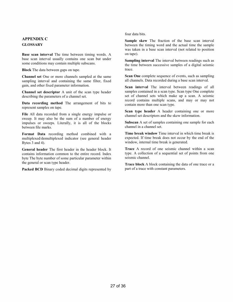
APPENDIX C GLOSSARY Base scan interval The time between timing words. A base scan interval usually contains one scan but under some conditions may contain multiple subscans.

Block The data between gaps on tape.

Channel set One or more channels sampled at the same sampling interval and containing the same filter, fixed gain, and other fixed parameter information.

Channel set descriptor A unit of the scan type header describing the parameters of a channel set.

Data recording method The arrangement of bits to represent samples on tape.

File All data recorded from a single energy impulse or sweep. It may also be the sum of a number of energy impulses or sweeps. Literally, it is all of the blocks between file marks.

Format Data recording method combined with a multiplexed/demultiplexed indicator (see general header Bytes 3 and 4).

General header The first header in the header block. It contains information common to the entire record. Index byte The byte number of some particular parameter within the general or scan type header.

Packed BCD Binary coded decimal digits represented by

four data bits.

Sample skew The fraction of the base scan interval between the timing word and the actual time the sample was taken in a base scan interval (not related to position on tape).

Sampling interval The interval between readings such as the time between successive samples of a digital seismic trace.

Scan One complete sequence of events, such as sampling all channels. Data recorded during a base scan interval.

Scan interval The interval between readings of all samples contained in a scan type. Scan type One complete set of channel sets which make up a scan. A seismic record contains multiple scans, and may or may not contain more than one scan type.

Scan type header A header containing one or more channel set descriptors and the skew information.

Subscan A set of samples containing one sample for each channel in a channel set.

Time break window Time interval in which time break is expected. If time break does not occur by the end of the window, internal time break is generated.

Trace A record of one seismic channel within a scan type. A collection of a sequential set of points from one seismic channel.

Trace block A block containing the data of one trace or a part of a trace with constant parameters.

28 of 36

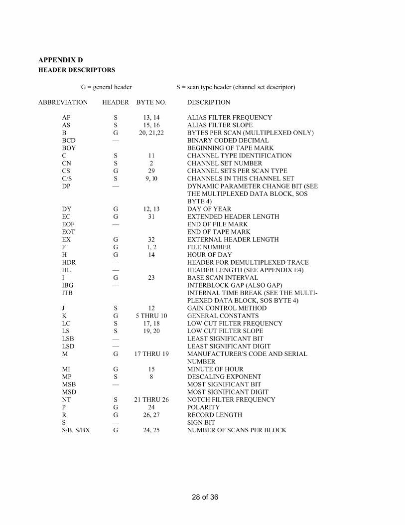
APPENDIX D HEADER DESCRIPTORS G = general header S = scan type header (channel set descriptor) ABBREVIATION HEADER BYTE NO. DESCRIPTION AF S 13, 14 ALIAS FILTER FREQUENCY AS S 15, 16 ALIAS FILTER SLOPE B G 20, 21,22 BYTES PER SCAN (MULTIPLEXED ONLY) BCD — BINARY CODED DECIMAL BOY BEGINNING OF TAPE MARK C S 11 CHANNEL TYPE IDENTIFICATION CN S 2 CHANNEL SET NUMBER CS G 29 CHANNEL SETS PER SCAN TYPE C/S S 9, l0 CHANNELS IN THIS CHANNEL SET DP — DYNAMIC PARAMETER CHANGE BIT (SEE THE MULTIPLEXED DATA BLOCK, SOS BYTE 4) DY G 12, 13 DAY OF YEAR EC G 31 EXTENDED HEADER LENGTH EOF — END OF FILE MARK EOT END OF TAPE MARK EX G 32 EXTERNAL HEADER LENGTH F G 1, 2 FILE NUMBER H G 14 HOUR OF DAY HDR — HEADER FOR DEMULTIPLEXED TRACE HL — HEADER LENGTH (SEE APPENDIX E4) I G 23 BASE SCAN INTERVAL IBG — INTERBLOCK GAP (ALSO GAP) ITB INTERNAL TIME BREAK (SEE THE MULTI- PLEXED DATA BLOCK, SOS BYTE 4) J S 12 GAIN CONTROL METHOD K G 5 THRU 10 GENERAL CONSTANTS LC S 17, 18 LOW CUT FILTER FREQUENCY LS S 19, 20 LOW CUT FILTER SLOPE LSB — LEAST SIGNIFICANT BIT LSD — LEAST SIGNIFICANT DIGIT M G 17 THRU 19 MANUFACTURER'S CODE AND SERIAL NUMBER MI G 15 MINUTE OF HOUR MP S 8 DESCALING EXPONENT MSB — MOST SIGNIFICANT BIT MSD MOST SIGNIFICANT DIGIT NT S 21 THRU 26 NOTCH FILTER FREQUENCY P G 24 POLARITY R G 26, 27 RECORD LENGTH S — SIGN BIT S/B, S/BX G 24, 25 NUMBER OF SCANS PER BLOCK

29 of 36

S/C S 12 EXPONENT OF SAMPLES PER CHANNEL IN THE BASE SCAN SE G 16 SECOND OF MINUTE SK G 30 NUMBER OF 32 BYTE SKEW FIELDS

SOS — START OF SCAN (MULTIPLEXED DATA BLOCK) SS — SAMPLE SKEW S/S — SAMPLES/SCAN

ST S 1 SCAN TYPE NUMBER ST/R G 28 SCAN TYPES PER RECORD

T — TIMING WORD (MULTIPLEXED DATA BLOCK) TF S 3, 4 FIRST TIMING WORD IN THIS CHANNEL

SET TE S 5, 6 END TIME OF THIS CHANNEL SET TN — DEMULTIPLEXED TRACE NO. (SEE TRACE HEADER) TW — TIME BREAK WINDOW (SEE DEMULTI- PLEXED DATA BLOCK, TRACE HEADER BYTES 13, 14 AND 15) TWI — TIME BREAK WINDOW INDICATOR (SEE MULTIPLEXED DATA BLOCK, SOS BYTE 4) Y G 3, 4 FORMAT CODE (DATA RECORDING METHOD) YR G 11 YEAR (LAST TWO DIGITS) Z G 26 RECORD TYPE

30 of 36

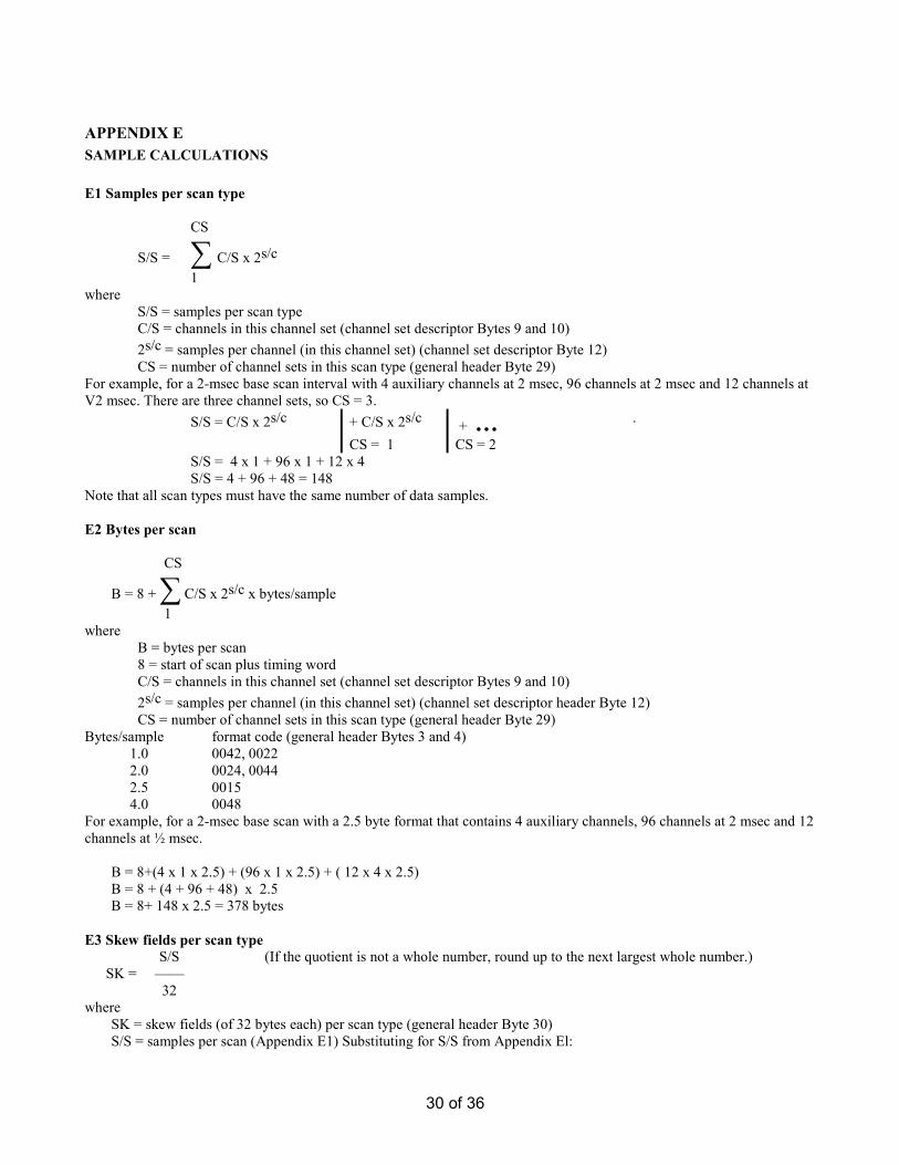
APPENDIX E SAMPLE CALCULATIONS E1 Samples per scan type

CS

S/S = ∑ C/S x 2s/c 1

where S/S = samples per scan type C/S = channels in this channel set (channel set descriptor Bytes 9 and 10) 2s/c = samples per channel (in this channel set) (channel set descriptor Byte 12) CS = number of channel sets in this scan type (general header Byte 29)

For example, for a 2-msec base scan interval with 4 auxiliary channels at 2 msec, 96 channels at 2 msec and 12 channels at V2 msec. There are three channel sets, so CS = 3. S/S = C/S x 2s/c + C/S x 2s/c + … .

CS = 1 CS = 2 S/S = 4 x 1 + 96 x 1 + 12 x 4 S/S = 4 + 96 + 48 = 148 Note that all scan types must have the same number of data samples. E2 Bytes per scan CS

B = 8 + ∑ C/S x 2s/c x bytes/sample 1 where

B = bytes per scan 8 = start of scan plus timing word C/S = channels in this channel set (channel set descriptor Bytes 9 and 10) 2s/c = samples per channel (in this channel set) (channel set descriptor header Byte 12) CS = number of channel sets in this scan type (general header Byte 29)

Bytes/sample format code (general header Bytes 3 and 4) 1.0 0042, 0022 2.0 0024, 0044 2.5 0015 4.0 0048 For example, for a 2-msec base scan with a 2.5 byte format that contains 4 auxiliary channels, 96 channels at 2 msec and 12 channels at ½ msec.

B = 8+(4 x 1 x 2.5) + (96 x 1 x 2.5) + ( 12 x 4 x 2.5) B = 8 + (4 + 96 + 48) x 2.5 B = 8+ 148 x 2.5 = 378 bytes

E3 Skew fields per scan type S/S (If the quotient is not a whole number, round up to the next largest whole number.) SK = —— 32 where

SK = skew fields (of 32 bytes each) per scan type (general header Byte 30) S/S = samples per scan (Appendix E1) Substituting for S/S from Appendix El:

31 of 36

CS

∑ C/S x 2s/c (If the quotient is not a whole number, 1 round up to the next largest whole number.) SK = ————————— 32

where

CS = the number of channel sets in each scan type (general header Byte 29) C/S = channels in this channel set (channel set descriptor Bytes 9 and 10) 2s/c = samples per channel in this channel set (channel set descriptor Byte 12).

For example, for a 2-msec base scan with 4 auxiliary channels at 2 msec, 96 channels at 2 msec and 12 channels at ~,6 msec 4 × 1+ 96 × 1 + 12 × 4 SK = ————————— 32 148 20 SK = —— = 4 —— roundup = 5 fields of 32 bytes each 32 32

E4 Total header length

HL = 32 x [ ST/R (CS + SK)+ 1 + EC + EX], where

HL = header length (bytes) ST/R = number of scan types per record (general header Byte 28) CS = number of channel sets per scan type (general header Byte 29) SK = skew fields per scan type (general header Byte 30) EC = extended header length (general header Byte 31) EX = external header length (general header Byte 32)

Example 1: For a system with a 2-msec base scan, 4 auxiliary channels at 2 msec, 96 channels at 2 msec, and 12 channels at Y2 msec

HL = 32 x (l x (3+5) + 1 + EC + EX) ST/R = 1 since there is only one scan type in this example, = 32 x (9) = 288 bytes + extended header + external header

E5 Filter slope calculation

Modern filters may not have a constant slope, so it is necessary to define this parameter. The slope is defined as the asymptote of effective performance as it would be in a constant slope filter. This slope is zero dB attenuation at the cut-off frequency and a specific attenuation at the beginning of the stop band. The chosen values are 40 dB for a low-cut filter and 60 dB for an anti-alias filter. Low-cut filter slope calculation. — 40 40 12.04 LS = ————— = ———————— = —————— log2 fLCO/f40 3.322 log10 fLCO/f40 log10 fLCO/f40

LS = low-cut filter slope (channel set descriptor Bytes 19 and 20), F40 = the frequency of 40 dB low-cut filter attenuation, fLCO = low-cut filter cut-off frequency usually 6 or 12 dB attenuation.

Alias-filter slope calculation. —

32 of 36

60 60 18.06 AS = ————— = ———————— = ————— log2 f6o/fACO 3.322 log10 f60/fACO log10 f60/fACO

AS = alias filter slope (channel set descriptor Bytes 15 and 16) F60 = the frequency of 60 dB alias-filter attenuation fACO = alias-filter cut-off frequency usually 3 or 6 dB attenuation

The resultant slope in the above calculations is rounded to the nearest whole number and is written in the channel set descriptor. E6 Calculation of byte offset from the beginning of the header block to a specific byte index in channel set descriptor i of scan type header j

Byte no. = 32 + index byte + 32 (CNi - l) + 32 (STj - l) (CS + SK) where

CNi = channel set number of interest index byte = byte number of interest in the channel set descriptor CS = number of channel sets per scan type (general header Byte 29).

STj = scan type of interest SK -skew fields per scan type (Appendix E3)

1 ≤ CNi ≤ CS

1 ≤ STj ≤ ST/R; i = 1, 2,...,ST/R

Example: For a 2 msec base scan system having 2 scan types: (1) 4 auxiliary channels at 2 msec plus 12 channels at ½ msec, and in the second scan type (2) 4 auxiliary channels at 2 msec plus 48 channels at 2 msec.

First calculate the samples per scan (S/S) per Appendix El and skew field (SK) per Appendix E3. CS

S/S = ∑C/S x 2sic

1 S/S = C/S x 2s/c + C/S x 2s/c CS = 1 CS = 2 = 4 x 1 + 12 x 4 S/S = 4 + 48 = 52. Note: It is not necessary to evaluate the samples per scan in the second scan type because all scan types must have the same number of samples.

Second, evaluate the skew fields per scan per Example 3. CS

∑ S/S (round up to the next 1 largest whole number), SK = ———— 32 52 20 SK = —— = 1 —— 32 32 Now, compute the header byte number of index Byte 11 of the second channel set in the second scan type.

33 of 36

Byte no. = 32 + 11 + 32 ( 2- 1) +32 ( 2 - 1) ( 2 + 2 ) Byte no. = 43 + 32 (1) + 32 (4) Byte no. = 203. E7 Calculation and use of MP

The MP parameter is provided to allow the dimensionless numbers recorded on tape to be "descaled" back to the instantaneous sample values in millivolts at the system inputs. MP is encoded in Byte 8 of each channel set descriptor in the scan type header. It is a sign and magnitude binary exponent. It can have any value between -31.75 and +31.75 in increments of 0.25.

In general, recording systems scale the input signal level in order to match the useful range of input levels to the gain-ranging amplifier. MP must account for all scaling (unless, as in the 4 byte hexadecimal case, the data recording method has sufficient range). MP CALCULATION

The calculation of MP for a data recording method is given by one of the following equations:

(1) MP = FS - PA - Cmax; for binary exponents, (2) MP = FS- PA – 2 x Cmax; for quaternary exponents, (3) MP = FS - PA – 4 x Cmax; for hexadecimal exponents (except the 4 byte excess 64 method), (4) MP = FS – PA - 4 (Cmax - 64); for excess 64 hexadecimal exponents,

where 2FS = Converter full scale (millivolts), 2PA= Minimum system gain,

and Cmax = maximum value of the data exponent. Cmax = 15 for binary exponents, = 7 for quaternary exponents, = 3 for hexadecimal exponents except excess 64; and = 127 for excess 64 exponents.

The term "minimum system gain" includes preamplifier gain and the minimum floating point amplifier gain. For

example, one system may use a preamplifier gain of 256 and a minimum floating point amplifier gain of one. The minimum system gain is 256 x 1 = 28, so PA=8. Another system may use a preamplifier gain of 320 and a minimum floating point amplifier gain of 0.8. In this case, the minimum system gain is 320 x 0.8 = 256 or 28 Again PA = 8.

PA may also account for any amplification needed to accommodate an analog to digital converter with a full scale value that is not a power of 2 in millivolts. For example, a 10 V (10,000 mV) converter may be preceded by an amplifier with a gain of 1.221 (10,000/8,192). This gain may be accounted for in PA. Alternatively, it could be considered part of the converter, making it appear to have a binary full scale. In either case, FS - PA must be a multiple of 0.25. JUSTIFICATIONS FOR THE EQUATIONS

The output of the analog-to-digital converter is written as the fractional portion of the data value. This is equivalent to

dividing the value by the full scale of the converter. In order to compensate for this, the data value recorded on tape must be multiplied by the full scale value of the converter (2FS). Thus FS appears in equations (1)-(4) with a positive sign.

The input signal was multiplied by the minimum system gain (2PA) which, as mentioned, includes any preamplification gain, minimum floating point amplifier gain, or analog-to-digital converter adjustment gain. The data recorded on tape must be divided by this minimum system gain; thus, PA appears in the equations with a negative sign.

Large input signals converted at minimum floating point amplifier gain are written on tape with the maximum exponent for the data recording method used. Likewise, small signals converted at full gain are written with the minimum exponent. The data as written have been multiplied by the exponent base raised to Cmax (or Cmax -64 in the excess 64 case). Thus Cmax appears in the equations with a negative sign. MP is a power of 2 so the quaternary and hexadecimal Cmax values are multiplied by 2 and 4, respectively (4C = 22C and 16c = 24C).

34 of 36

EXAMPLES

Note: In the following examples, all logarithms are base 10. Example 1

Assume: quaternary data recording method, converter full scale = 8192 m V, preamplifier gain = 320, and minimum floating point amplifier gain = 0.8. Then

Cmax = 7, FS = log 8192 / log 2 = 13, PA = log (320 x 0.8) / log 2 = 8.

and MP = 13 - 8 - 2 x 7 = -9.

Example 2

Assume: binary data recording method, convener full scale = 10 volts, preamplifier gain = 128, and minimum floating point amplifier gain = 1.0. Then

Cmax = 15, FS = log 10000 / log 2 = 13.287 .... PA = log 128 / log 2 = 7,

and MP = 13.287... - 7 – 15 = -8.712 ....

But MP must be a multiple of 0.25. This can be achieved by changing the preamplifier gain to 131.39. Then PA = log 131.39 / 1og 2 = 7.037 and MP = 13.287 . . . -7.037 . . . -15 = -8.75.

MP could be made a whole number by changing the preamplifier gain to 156.25. Then PA = log 156.25/log 2 = 7.287 and MP= 13.287 . . .-7.287 . . . -15 = -9.

Note that this is equivalent to preceding the conventer with an amplifier of gain 1.220... thus making the converter appear to have a full scale value of 8192 mV. Then

FS = log 8192 / 1og 2 = 13, PA = log 128 / log2 = 7,

and MP = 13 – 7 – 15 = -9.

Example 3

Assume: hexadecimal (1 or 2 byte) data recording method, convener full scale - 8192 mV, preamplifier gain = 256, and minimum floating point amplifier gain = 1.0. Then

Cmax = 3, FS = log 8192 / 1og 2 = 13, PA = log 256 / log2 = 8,

and MP = 13 - 8 - 4 x 3 = -7.

Note: In the 4 byte hexadecimal case, it is expected that MP will generally be recorded as zero because of the large range of the number system of this data recording method. Nonetheless, equation 4 must still be valid:

MP = FS - PA – 4 x ( Cmax – 64 ). If MP = 0, then

FS- PA = 4 ( Cmax- 64 ). Since Cmax is always an integer, FS - PA must be a multiple of 4. Note: The data recording method (binary, quaternary, or hexadecimal) does not indicate the type of floating point amplifier used. Any gain ranging amplifier and converter outputs can be convened to any of the data recording methods.

USE OF MP

As indicated in the descriptions of the data recording formats, MP is applied by multiplying the recorded data by 2MP.

35 of 36

E8 Calculation of the byte offset from the beginning of the header block to the skew information byte for channel k of channel set i of scan typej For clarity, the equation is given on several lines. The terms on each line are explained. SS OFFSET = 32 (general header) + 32(STj- 1) (CS + SK) (all previous scan type headers) + 32 (CS) (channel set descriptors in scan type header j) CNi- 1

+ ∑ C/S x 2s/c (samples in the base scan for 1 all previous channel sets in this scan type) + k (position of channel in this channel set) Where

STj = scan type of interest, CS = number of channel sets per scan type (general header Byte 29), SK = number of skew fields per scan type (Appendix E3), CNi = channel set number of interest, C/S = channels in this channel set (channel set descriptor Bytes 9 and 10), and 2s/c = samples per channel of this channel set in a base scan (channel set descriptor Byte 12).

Note that if there are multiple subscans of a channel set within a base scan (i.e., 2s/c greater than one), a skew information byte is written for each sample in each subscan.

The above equation accounts for multiple subscans of previous channel sets, but it determines the location of the skew information byte of channel k in the first subscan only of channel set i. Skew information for subsequent subscans can be obtained in two ways:

(1) Add multiples of C/S to the computed offset to obtain the offset to the byte of interest; or (2) Add multiples of 2-s/c to the value of the skew information byte obtained for the first sub-scan.

For example, assume there are two .scan types with three channel sets, as follows: Scan type 1:

channel set 1 — 4 channels at 4 msec (1 subscan per base scan) channel set 2 — 24 channels at 2 msec (2 subscans per base scan) channel set 3 — 12 channels at l msec (4 subscans per base scan)

Scan type 2: Channel set 1 — 4 channels at 4 msec (1 subscan per base scan) Channel set 2 — 48 channels at 2 msec (2 subscans per base scan) Channel set 3 — 0 channels (dummy).

The offset to the skew information byte for channel 11 of channel set 2 in scan type 2 is computed below. The number of skew fields (Appendix E3) is:

CS

∑C/S x 2s/c = 4 + 24 x 2 + 12 x 4 = 100

1 —————— = —— 32 32 or 4 (rounded up).

36 of 36

CNi- 1

SS offset = 32 + 32(STj- 1)(CS + SK) + 32(CS) + ∑ C/S x 2S/C + k 1 = 32 + 32(2 - 1)(3 + 4) + 32(3) + 4 + 11 = 367.

The position of the skew information byte for the second subscan of channel 11 in this scan is: 367 + 48 = 415. E9 Calculation of the number of bytes per block for a gapped multiplexed record

Bytes per block = (S/B x 2S/BX) × B where

S/B x 2S/BX = scans per block (general header Bytes 24 and 25) B = bytes per scan (general header Bytes 20, 21, and 22).

Note: S/B and S/BX are written in the header as binary numbers; whereas B is represented as 6 packed BCD digits. Assume, as in example E2, that there are 378 bytes per scan. Further assume that S/BX is 2 and S/B is 173. Then ( S/B x 2S/BX ) x B = 173 x 22 x 378, and bytes per block = 261,576. E10 Determination of scans per block subject to block size limits S/B and S/BX will normally be chosen to result in the largest block (fewest gaps) possible without exceeding a predetermined limit. This is accomplished by selecting S/BX to be just large enough that 2S/BX is within a factor of 256 of the maximum number of scans allowed. Maximum number of scans = integer portion of block limit per bytes per scan.

Max number S/BX = log2 ——————— rounded up, 256 Max number of scans S/B = —————————— rounded down. 2S/BX

For example, assume that there are 378 bytes per scan and the block size may not exceed 250,000 bytes. Int of 250,000 661 Max scans = ————— S/B = ——— rounded down 378 22 = 661 = 165; 661 Block length = 165 x 22 x 378, S/BX = Log2 —— rounded up, = 249,480 bytes. 256 =2;