Embed Size (px)
Citation preview

From Topographic Maps to Digital Elevation Models
Anne Graham
Daniel Sheehan
MIT Libraries
IAP 2013

Which Way Does the Water Flow?
A topographic map shows relief features or surface configuration of an area.

A hill is represented by lines of
equal elevation above mean
sea level. Contours never cross.

Elevation values are printed in several places along these lines.
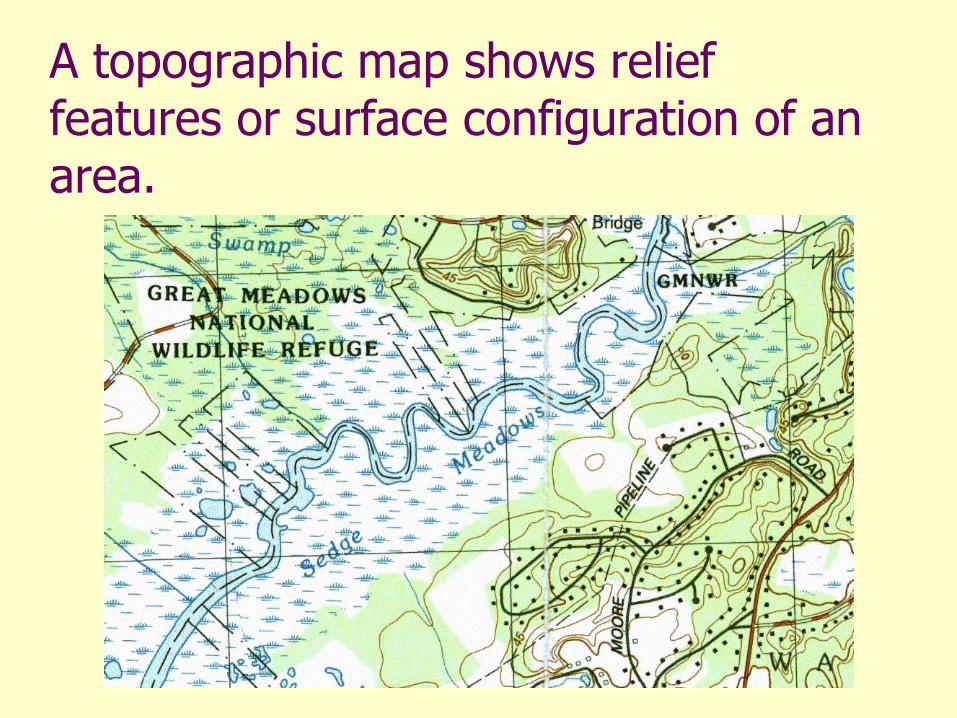
Contours that are very close together represent steep slopes.

Widely spaced contours or an absence of contours means that the ground slope is relatively level.

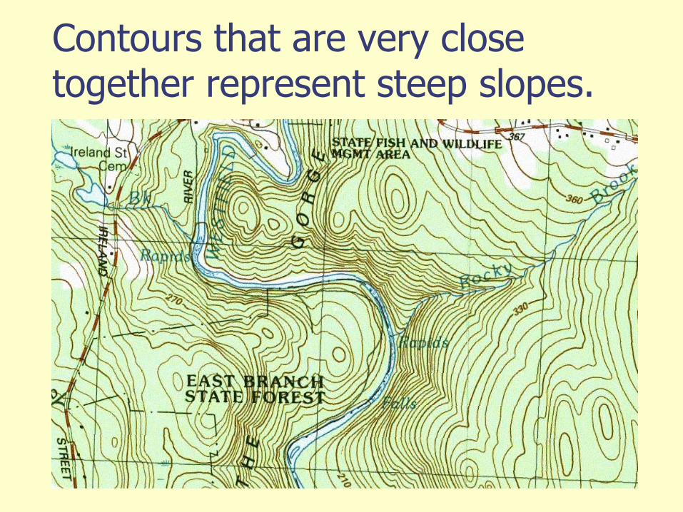
The elevation difference between adjacent contour lines, called the contour interval, is selected to best show the general shape of the terrain. A map of a relatively flat area may have a contour interval of 10 feet or less.
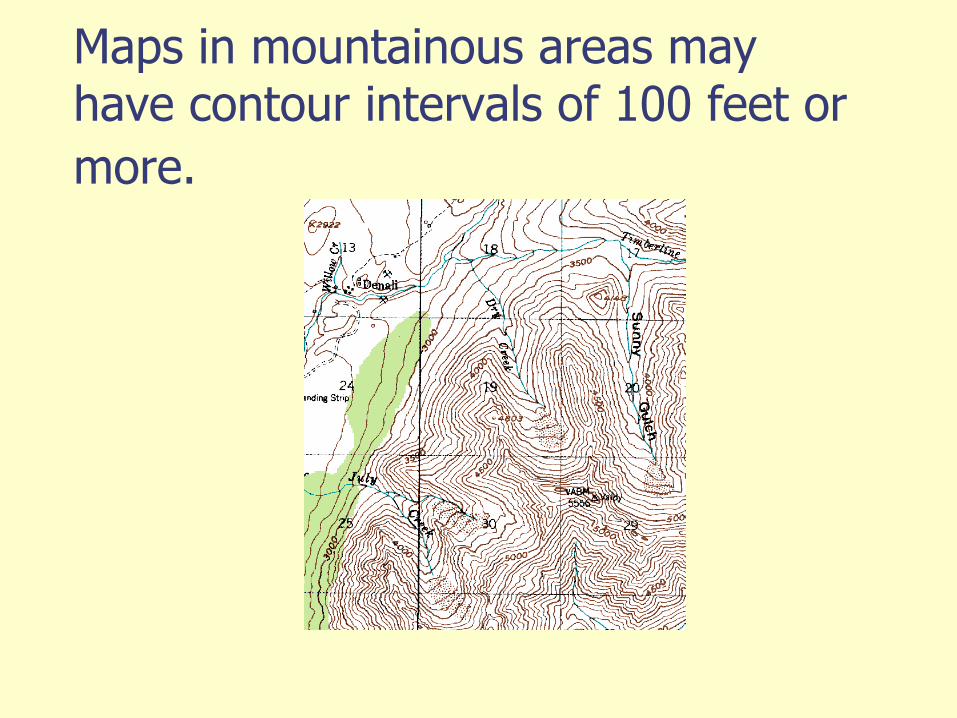
Maps in mountainous areas may have contour intervals of 100 feet or
more.

A city can be overlain on a
topographic map.

A bench mark is a surveyed elevation point.

Contour lines point up stream.

United States Geological Survey Topographic Map Symbols Explained
http://erg.usgs.gov/isb/pubs/booklets/symbols/

Digital Elevation Models
Using elevation data in raster format in a GIS Daniel Sheehan Senior GIS Specialist MIT Libraries [email protected] [email protected] X2-1475

What is a Digital Elevation Model (DEM)?
Digital representation of topography
Cell based with a single elevation representing the entire area of the cell

Basic storage of data
340 335 330 340 345
337 332 330 335 340
330 328 320 330 335
328 326 310 320 328
320 318 305 312 315
DEM as matrix of elevations with a uniform cell size

Adding geography to data
340 335 330 340 345
337 332 330 335 340
330 328 320 330 335
328 326 310 320 328
320 318 305 312 315
Xmin, Ymin – XY are in projected units
Xmax, Ymax
Cell index number x cell size defines position relative to Xmin, Ymin and Xmax, Ymax and infers An exact location

DEM in Grid Ascii format
ncols 2218 nrows 2013 xllcorner 203315.48791178 yllcorner 905650.13397789 cellsize 8.8654680523268 NODATA_value -9999 5.27725 55.36783 55.52513 55.79526 … 57.22343 57.69468 58.06146 58.32586 … …
Uses of DEMs
Determine characteristics of terrain
Slope, aspect
Watersheds
drainage networks

Scale in DEMs
Scale determines resolution (cell size)
Depends on source data
Resolution determines use of DEM and what spatial features are visible

Nine 30 meter cells within one 90 meter cell

Estimating slopes in a DEM
Slopes are calculated locally using a neighborhood function, based on a moving 3*3 window
Distances are different in horizontal and vertical directions vs diagonal
Only steepest slopes are used
1.41… 1 1.41…
1 0 1
1.41… 1 1.41…
* cell size

Flow Direction
Useful for finding drainage networks and drainage divides
Direction is determined by the elevation of surrounding cells Water can flow only into one cell – the cell
with the lowest elevation surrounding the current cell
Water is assumed to flow into one other cell, unless there is a sink GIS model assumes no sinks

Flow direction in a DEM
340 335 330 340 345
337 332 325 335 340
330 328 320 330 335
328 326 310 320 328
320 318 305 312 315
Flow directions for individual cells

32 64 128
16 Source
Cell 1
8 4 2

Flow direction in a DEM
2 2 4 8 8
2 2 4 8 8
2 2 4 8 8
2 2 4 8 8
1 1 4 16 16
Flow directions for individual cells
Finding watersheds …
Begin at a source cell of a flow direction database, derived from a DEM (not from the DEM itself
Find all cells that flow into the source cell
Find all cells that flow into those cells.
Repeat …
The resulting watershed is generalized, based on the cell size of the DEM

Watersheds …
Contour lines (brown) Drainage (blue) Watershed boundary (red)

Flow accumulation
The number of cells, or area, which contribute to runoff of a given cell
The accumulation function determines the area of a watershed that contributes runoff to any given cell – which cells, or area, is upstream and/or upslope of a given cell

Flow direction in a DEM
340 335 330 340 345
337 332 325 335 340
330 328 320 330 335
328 326 310 320 328
320 318 305 312 315
Flow directions for individual cells

Flow accumulation in a DEM
0 0 0 0 0
0 1 3 1 0
0 1 8 1 0
0 1 13 1 0
0 2 24 2 0
Flow accumulation for individual cells

Flow accumulation as drainage network
Drainage network as defined by cells above threshold value for region.

Map Projections
Displaying the earth on 2 dimensional maps
The “World From Space” Projection from ESRI, centered at 72 West and 23 South. This approximates the view of the earth from the sun on the winter solstice at noon in Cambridge, MA

Map projections …
Define the spatial relationship between locations on earth and their relative locations on a flat map
Are mathematical expressions
Cause the distortion of one or more map properties (scale, distance, direction, shape)

Classifications of Map Projections
Conformal – local shapes are preserved
Equal-Area – areas are preserved
Equidistant – distance from a single location to all other locations are preserved
Azimuthal – directions from a single location to all other locations are preserved

Another classification system
Planar
Cylindrical
Conic
By the geometric surface that the sphere is projected on:

Planar surface
Earth intersects the plane on a small circle. All points on circle have no scale distortion.

Cylindrical surface
Earth intersects the cylinder on two small circles. All points along both circles have no scale distortion.

Conic surface
Earth intersects the cone at two circles. all points along both circles have no scale distortion.

Scale distortion
Scale near intersections with surface are accurate
Scale between intersections is too small
Scale outside of intersections is too large and gets excessively large the further one goes beyond the intersections

Why project data?
Data often comes in geographic, or spherical coordinates (latitude and longitude) and can’t be used for area calculations in most GIS software applications
Some projections work better for different
parts of the globe giving more accurate
calculations

Some projection parameters
Standard parallels and meridians – the place where the projected surface intersects the earth – there is no scale distortion
Central meridian – on conic projects, the center of the map (balances the projection, visually)

1/6 Rule in Conic Projections
1st standard parallel is 1/6 from southern edge of mapping area,
2nd standard parallel is 1/6 from northern edge of the mapping area
Central Meridian is mid point in the east-west extent of the map

Conic projection for US
45 N
29 N
97 W
Northern edge of map is 49 N, southern edge is 25 S. Range is 24 degrees. 1/6 = 4 degrees.

Conic projection implemented
Contiguous 48 states represented as we are accustomed to seeing them and areas are approximately accurate

Datums
Define the shape of the earth including:
Ellipsoid (size and shape)
Origin and Orientation
Aligns the ellipsoid so that it fits best in the region you are working

How to choose projections
Generally, follow the lead of people who make maps of the area you are interested in. Look at maps!
State plane is a common projection for all states in the USA Conic and UTM variants
UTM is commonly used and is a good choice when the east-west width of area does not exceed 6 degrees

UTM projection
Universe Transverse Mercator
Conformal projection (shapes are preserved)
Cylindrical surface
Two standard meridians
Zones are 6 degrees of longitude wide

UTM projection
Scale distortion is 0.9996 along the central meridian of a zone
There is no scale distortion along the the standard meridians
Scale is no more than 0.1% in the zone
Scale distortion gets to unacceptable levels beyond the edges of the zones

UTM zones
Numbered 1 through 60 from Longitude 180
State Plane Coordinate System
System of map projections designed for the US
It is a coordinate system vs a map projection (such as UTM, which is a set of map projections)
Designed to minimize distortions to 1 in 10000
2 sets of projections are used, UTM and Lambert Conformal Conic

Projecting Grids from spherical coordinates
Cells are square in a raster GIS but: Size of cell changes with latitude – for
example, 1 minute (of arc) 1854 meters by 1700 meters in Florida and 1854 meters by 1200 meters in Montana.
Problems: Impossible to match cells one to one in two
different projections – resampling (CUBIC for elevation data) or nearest neighbor for categorized data

In ArcGIS …
Arctoolbox contains the projection tools
Define a projection
Project a shapefile or grid to a new projection
Arcmap
Change the projection for display and calculation

Things to do before the exercise:
In Windows, create a new folder under your username on the T:\ folder if one doesn’t already exist.
Start Arcmap. In Arcmap, click on tools then Extension. Check the box for Spatial Analyst and close the window. Again click on tools and then Customize Mode. Again, check the box for the Spatial Analyst toolbox and close the window.