Diffusion Magnetic Resonance as the Basis of Novel

Biomarkers Using Multidimensional Statistics

in the Brain

PhD thesis

Gyula Gyebnár

János Szentágothai Doctoral School

Semmelweis University

Supervisor: Lajos Rudolf Kozák MD, PhD

Official reviewers: András Jakab, MD, PhD

Pál Kaposi Novák, MD, PhD

Head of the Final Examination Committee:

Kinga Karlinger, MD, PhD

Members of the Final Examination Committee:

Miklós Krepuska, MD, PhD

Regina Deák-Meszlényi, PhD

Budapest

2020

Table of contents

Table of contents 2

List of abbreviations 6

I. Introduction 8

1. Foreword 8

2. Diffusion Magnetic Resonance Imaging 10

2.1 Basics of diffusion MRI 10

2.2 Diffusion MRI approaches in neuroimaging 12

2.2.1 Diffusion weighted imaging 13

2.2.2 Diffusion tensor imaging 14

2.2.3 Outlook on dMRI methods beyond DTI 19

2.2.4 Imaging, correction, and data processing in dMRI 22

3. Statistics in brain MRI studies 24

3.1 Univariate statistics 24

3.2 The problem of multiple comparisons 25

3.3 Multivariate approaches 26

4. The Mahalanobis‒distance 28

4.1 Definition 28

4.2 The Mahalanobis‒distance in neuroimaging 29

4.3 Statistical inference based on critical values 30

5. Research topics – Clinical importance 32

5.1 Mild Cognitive Impairment 32

5.1.1 MRI diagnostics of MCI 32

5.1.2 The role of DTI in MCI diagnostics 33

5.2 Drug resistant epilepsies (DREs) 33

5.2.1 DTI in the diagnosis of epilepsy 34

II. Aims 35

1. DTI and Mild Cognitive Impairment 35

2. Mahalanobis‒distance in MCD lesion detection 35

III. Materials and Methods 36

1. DTI and Mild Cognitive Impairment 36

3

1.1 Study data and Participants 37

1.2 Preprocessing and diffusion tensor fitting 40

1.3 Voxelwise analysis 40

1.3.1 Voxelwise correlation analysis 41

1.3.2 Voxel‒based between group statistical analysis 42

1.3.3 Visualization 43

1.4 ROI‒based statistics 43

1.4.1 ROI‒based correlation analyses and between‒group comparisons 43

1.4.2 ROI‒based logistic regression analysis for a combined cortical thickness

and DTI based differentiation between study groups 43

2. Mahalanobis‒distance in MCD lesion detection 45

2.1 Study data and participants 45

2.2 Data processing 46

2.3 Independent automatic evaluation of MCDs 48

2.4 Mahalanobis‒distance related calculations 48

2.5 Simulations 49

2.5.1 Simulations with Gaussian distributions 49

2.5.2 Simulations with real eigenvalues 52

2.6 Leave‒one‒out examination of controls 53

2.6.1 Cluster description based on tissue probability maps (TPMs) 54

2.7 Representative cases of MCDs 55

IV. Results 56

1. DTI and Mild Cognitive Impairment 56

1.1 Voxelwise analyses 56

1.1.1 Voxelwise correlation analysis 56

1.1.2 Voxelwise ANOVA and between-group differences 60

1.2 ROI‒based analyses 64

1.2.1 ROI‒based correlations with the results of the neuropsychology tests 64

1.2.2 ROI‒based between group differences 66

1.3 ROI‒based logistic regression analysis: combined cortical thickness and DTI‒

based differentiation between study groups 67

1.3.1 Differentiation between aMCI subjects and healthy controls 68

1.3.2 Differentiation between naMCI subjects and healthy controls 72

4

1.3.3 Differentiation between aMCI and naMCI subjects 76

2. Mahalanobis‒distance in MCD lesion detection 80

2.1 SMVND simulations 82

2.1.1 False Positives 82

2.1.2 True positive rates and hit rates 82

2.2 Real Eigenvalue simulations 84

2.2.1 False Positives 84

2.2.2 True positive rates and hit rates 84

2.3 Real data examinations 87

2.3.1 Leave‒one‒out analysis of controls 87

2.3.2 Patient Examination 89

V. Discussion 91

1. DTI and Mild Cognitive Impairment 91

1.1 Functional‒structural correlations 91

1.2 Impairments in aMCI patients compared to naMCI patients and healthy controls

93

1.3 Impairments in naMCI patients compared to control subjects 94

1.4 Differentiation between study groups by logistic regression 94

1.5 On the value of DTI measurements in MCI and AD 95

1.6 Limitations of the study 96

2. Mahalanobis‒distance in MCD lesion detection 97

2.1 Multidimensional approaches 97

2.2 On information sources and dimensionality considerations 98

2.3 Simulation results 99

2.4 Leave‒one‒out examination of controls 101

2.5 Patient examinations 101

2.6 Limitations 105

VI. Conclusions 107

1. DTI and Mild Cognitive Impairment 107

2. Mahalanobis‒distance in MCD lesion detection 107

3. General conclusions 108

VII. Summary 109

5

VIII. Összefoglalás 110

References 111

List of publications 132

1. Articles related to the thesis 132

2. Other articles 132

Acknowledgements 133

Reprints of publications related to the thesis 134

Supplementary material 135

6

List of abbreviations

2D Two Dimensional

3D Three Dimensional

3T Three Tesla

ACE Addenbrooke’s Cognitive

Examination

AD Alzheimer’s Disease

ADC Apparent Diffusion Coefficient

AFROC Alternative Free-Response

Receiver-Operator Characteristics

aMCI Amnestic Subtype of Mild

Cognitive Impairment

ANOVA Analysis of Variance

AUC Area Under the Curve

BOLD Blood Oxygen Level

Dependent (signal)

CHARMED Composite Hindered and

Restricted Model of Diffusion

CNR Contrast‒to‒Noise Ratio

CNS Central Nervous System

CSF Cerebrospinal Fluid

CSD Constrained Spherical

Deconvolution

D2 Squared Mahalanobis‒Distance

DARTEL Diffeomorphic Anatomical

Registration using Exponentiated Lie

Algebra

DDF Diffusion Displacement Function

DKI Diffusional Kurtosis Imaging

dMRI Diffusion Magnetic Resonance

Imaging

DNT Disembryoplastic Neuroepithelial

Tumor

DRE Drug Resistant Epilepsy

DSI Diffusion Spectrum Imaging

DTI Diffusion Tensor Imaging

DWI Diffusion Weighted Imaging

EPI Echo Planar Imaging

FA Fractional Anisotropy

FCD Focal Cortical Dysplasia

FDR False Discovery Rate

FLAIR Fluid Attenuated Inversion

Recovery

fMRI Functional Magnetic Resonance

Imaging

fODF fiber Orientation Distribution

Function

FOV Field Of View

FPR False Positive Rate

FWE Family‒Wise Error Rate

FWHM Full Width at Half Maximum

GLM General Linear Model

GM Grey Matter

HARDI High Angular Resolution

Diffusion Imaging

HTP Heterotopia

HME Hemimegalencephaly

JHU Johns Hopkins University

LEAT Long‒Term Epilepsy‒

Associated Tumor

MD Mean Diffusivity

7

MCI Mild Cognitive Impairment

MCD Malformation of Cortical

Development

MNI Montreal Neurological Institute

MMSE Mini Mental State

Examination

MRI Magnetic Resonance Imaging

naMCI Non‒Amnestic Subtype of

Mild Cognitive Impairment

NODDI Neurite Orientation Dispersion

and Density Imaging

PAL Paired Associates Learning

PET Positron Emission Tomography

PFGSE Pulsed Field Gradient Spin

Echo

PMG Polymicrogyria

QSI q‒Space Imaging

RAVLT Rey Auditory Verbal

Learning Test

RD Radial Diffusivity

RESTORE Robust Estimation of

Tensors by Outlier Rejection

ROC Receiver‒Operator

Characteristics

ROI Region of Interest

SD Standard Deviation

SE Spin Echo

SMVND Standard Multivariate Normal

Distribution

T1 and T2 Characteristic Relaxation

Time for Longitudinal and Transverse

Magnetization

TBI Traumatic Brain Injury

TBSS Tract‒Based Spatial Statistics

TFCE Threshold‒Free Cluster

Enhancement

TE Echo Time

TI Inversion Time

TPM Tissue Probability Map

TPR True Positive Rate

TPRB True Positive Rate Binary

TR Repetition Time

VBA Voxel‒Based Analysis

VBM Voxel‒Based Morphometry

VLOM (Verbal Fluency + Language

Score / Orientation + Memory Score)

Ratio in the ACE

VLPFC Ventrolateral Prefrontal

Cortex

WM White Matter

8

I. Introduction

1. Foreword

The development of magnetic resonance imaging (MRI) in the last two decades have

propelled the investigation of the central nervous system (CNS) at an unprecedented rate.

With the increasing availability of high‒quality equipment and the inventions of novel

imaging and processing techniques, MRI has been pushed to the forefront of brain

research, facilitating several large‒scale initiatives, such as the Human Connectome

Project [1-3], the Human Brain Project [4], or the UK Biobank Project [5], and imaging

was also given due attention in the Hungarian Brain Research Program (NAP).

The ever‒growing amount of multimodal brain imaging data, especially with the

introduction of diffusion and functional MRI, has been driving the development and use

of novel processing and statistical methods. Since different modalities, even distinct MR

contrast mechanisms, provide complementary information on brain structure and

function, methods combining data from various approaches could aim for more accuracy

and sensitivity by leveraging their advantages.

The work behind the present Thesis was aimed at developing methods and new

biomarkers using combinations of state of the art neuroimaging techniques with diffusion

MRI. Although the machine learning‒based methods for image processing and analysis

(some of which are referred to with the alluring term ‘radiomics’), that received an

exponentially growing interest in the past few years are promising optimized, data‒based,

automated feature selection, their general use is still hampered by, among other factors,

the need for vast amounts of well‒annotated training data. The author firmly believes that

knowledge‒driven studies addressing specific research questions, such as the ones

presented in this Thesis, still hold merit, at least by forming basis for and interpreting the

results of such endeavors.

In the first study of the thesis, conventional whole brain two sample parametric

statistics and correlation analyses, followed by subsequent white matter region‒level

analyses were used to identify the brain structures where mild cognitive impairment

inflicts substantial alterations on the diffusion profile, and measurements from these

9

structures were fed into stepwise logistic regression. Our results demonstrated that

combining volumetry measurements from anatomical scans with robust region‒level

diffusion tensor metrics significantly aids distinguishing patients from healthy subjects,

and improves the differentiation between amnestic and non‒amnestic subtypes of mild

cognitive impairment even more.

In the second study a novel approach was proposed and demonstrated for single

subject whole brain voxel‒level analyses, based on the squared Mahalanobis‒distance

with analytically derived critical values. The problem of identifying epilepsy‒related

structural abnormalities was implemented as a data‒driven detection problem, treating

diffusion tensor eigenvalues from lesion voxels as outliers compared to the distribution

derived from healthy controls. The expected detection rate and sensitivity to different

effect strengths and lesion volumes was explored through simulations, and verified in

select cases with malformations of cortical development.

10

2. Diffusion Magnetic Resonance Imaging

2.1 Basics of diffusion MRI

Diffusion magnetic resonance imaging (dMRI) is a general term referring to a group

of methods widely used for the non‒invasive examination of biological samples and

porous materials [6-8]. The term diffusion in dMRI refers to the random thermal motion

of water molecules in the extracellular space, described by Einstein’s theory: the

ensemble average translation is proportional to the elapsed time, and the ratio is called

the diffusion coefficient:

< (𝒓′ − 𝒓)2 >= 6𝐷𝑡 (𝐸𝑞. 1)

By using spatially varying magnetic fields (referred to as diffusion encoding

gradients), the magnetic resonance (MR) signal can be made sensitive to the microscopic

motion of water molecules [9, 10]. An ‘encoding gradient’ means that the magnetic field

component parallel to the polarizing field (B0) changes linearly across the sample space.

This is achieved by generating additional magnetic fields much smaller than B0, using

coils with special geometry. The gradient of the parallel component, denoted as g,

describes the change in magnetic field along the direction of the pulsed magnetic field.

By employing the encoding gradient, the Larmor frequencies (ω) of the nuclear magnetic

spins of water molecules (at coordinates r) also vary linearly along the direction of g:

𝜔(𝒓) = 𝛾𝐵0 + 𝛾𝒈 ∙ 𝒓 (𝐸𝑞. 2)

where γ is the gyromagnetic ratio. The use of the gradient over an evolution time t

results in an accumulated phase shift dependent on the position: 𝛥𝜑 = exp (𝑖𝛾𝒈 ∙ 𝒓𝑡).

In practice, most diffusion‒weighted MR sequences follow the Stejskal‒Tanner

encoding scheme [11] with a spin echo (Fig 1).

11

Fig 1 The Stejskal‒Tanner diffusion encoding scheme

Two identical diffusion encoding gradients (g) are used, with pulse length δ and diffusion time Δ. The 180°

RF pulse inverts the phase shift accumulated during the first gradient, thereby the second gradient

effectively rewinds the phases for stationary spins, but displacement along the direction of the gradient

results in remaining phase error.

Diffusion encoding is achieved by two identical pulsed gradients preceding and

following a 180° spin‒echo (SE) pulse. The SE‒pulse inverts the phase shift resulting

from the first gradient, so the second one completely recovers the phase for stationary

spins. For moving spins, with displacement R along the direction of the gradients, the

remaining phase error is Φ = 𝛾𝐺𝛿𝑅, with gradient pulse strength G = |g|, and pulse length

δ. The signal attenuation in a pulsed field gradient spin echo (PFGSE) sequence with

short, rectangular gradient pulses and echo time TE, as shown in [11], is:

𝐴(𝑇𝐸) = exp [−𝛾2𝐺2𝐷𝛿2 (𝛥 −𝛿

3)] (𝐸𝑞. 3)

Parameters describing the diffusion encoding are generally merged in order to

simplify the equation, defining the so‒called b‒value:

𝑏 = 𝛾2𝐺2𝛿2 (𝛥 −𝛿

3) (𝐸𝑞. 4)

12

As diffusion means the flux of particles through a surface during a given period of

time, its’ dimension is in the form of [area/time]. In order for the exponent –bD to be

dimensionless, b is expressed as [time/area]. In practice, b‒values are given in units of

𝑠/𝑚𝑚2, in the range of 0 – 10000. From the attenuated signal (Sb) corresponding to a

given b‒value, and a reference measurement (S0) without diffusion encoding, the apparent

diffusion coefficient (ADC) along the direction of the gradient can be calculated:

𝐴𝐷𝐶(𝑏) =ln (

𝑆𝑏

𝑆0)

𝑏(𝐸𝑞. 5)

It is important to note, that the mono‒exponential signal attenuation in (Eq.3) is only

accurate for rectangular gradient pulses and free diffusion. In practice, gradient shapes

are trapezoidal and the b‒values given by MR scanners are calculated slightly differently,

accounting for the finite rise times and the auxiliary effects of imaging gradients as well.

Free diffusion means that the displacement of water molecules can be described as a

simple Gaussian process (i.e. the probability distribution of spin displacement can be

described with a three dimensional Gaussian function). Strictly, this is only true for pure,

homogenous liquid samples with infinite size, but the approximation also holds for water

molecules in the extracellular space with most b‒values used in human studies, except for

those specifically chosen to measure the non‒Gaussian behavior of the dMRI signal (see

subsection 2.2.3).

2.2 Diffusion MRI approaches in neuroimaging

Even though diffusion only results in displacements on the microscopic scale, the

degree, at which water molecules can move in the three‒dimensional space of the

extracellular environment may be hindered due to the physical arrangement of obstacles

in one, two, or all three directions, resulting in restricted, and in many cases anisotropic

diffusion [12]. Therefore, the measured signal attenuation in biological samples reflects

properties of tissue microstructure [6-8]. Measurement and data processing approaches

can be described according to the level of information extracted about the diffusion

pattern. By measuring ADC‒values in several directions, one can define the diffusion

profile as a three dimensional surface describing the orientation distribution of the

observed displacement in each voxel (Fig 2).

13

Fig 2 Diffusion profiles of several voxels in the deep parieto‒occipital white matter

Apparent diffusion coefficients in each measured direction can be used to construct 3D surfaces, visualizing

the orientation distribution of the observed mean displacement of extracellular water molecules. The

difference between white matter structures with a single main orientation (e.g. the callosal fibers on the

middle on the left side), with two or three orientations (on the bottom in the middle and the right side), in

gray matter with no clear maxima (lower left corner), and in the cerebrospinal fluid (CSF ‒ upper left

corner) can be measured and visualized.

2.2.1 Diffusion weighted imaging

The simplest approach of dMRI, called diffusion weighted imaging (DWI), quickly

gained interest in the clinical field for its superior sensitivity detecting cerebral ischemia

through the restricted diffusion signal of cytotoxic edema, appearing in minutes after the

occlusion [13]. DWI has also been proven useful in onco‒radiology. In DWI, diffusion‒

encoding gradients are applied separately in three perpendicular directions; restricted

diffusion can be identified as high signal intensity after averaging the corresponding

images. Due to averaging, directional, and therefore anisotropy information is not

extracted; DWI can be viewed as measuring only the volume enclosed by the diffusion

profile (with the three orthogonal directions, the corresponding surface is a cuboid). By

14

acquiring a reference image and calculating the ADC‒values from the averaged images,

other biological and physics‒related phenomena (e.g. differences in T2‒relaxation times)

can be disentangled from the effects of the diffusion process.

2.2.2 Diffusion tensor imaging

The most widely known (and simplest) technique, capable of handling anisotropy

information, used in both clinical neuroradiology and for innumerable research questions

about the CNS, is diffusion tensor imaging (DTI) [14, 15]. Since DTI was the method of

choice in both research projects of the present Thesis, this section contains a detailed

explanation of the approach, with emphasis on its strengths and limitations.

In the DTI representation, the 3D Gaussian model uses a 3‒by‒3 tensor D to describe

diffusion anisotropy, instead of a scalar ADC:

𝑫 = [

𝐷𝑥𝑥 𝐷𝑥𝑦 𝐷𝑥𝑧

𝐷𝑦𝑥 𝐷𝑦𝑦 𝐷𝑦𝑧

𝐷𝑧𝑥 𝐷𝑧𝑦 𝐷𝑧𝑧

]

Using the observed properties of molecular diffusion, the tensor describing the

physical process must be real and symmetric, therefore Dxy = Dyx, Dxz = Dzx, and

Dyz = Dzy. By writing the diffusion encoding b‒vectors in matrix format, and utilizing this

symmetry, (Eq.5) takes the following form for DTI:

ln (𝑆𝒃

𝑆0) = −(𝑏𝑥𝑥𝐷𝑥𝑥 + 2𝑏𝑥𝑦𝐷𝑥𝑦 + 2𝑏𝑥𝑧𝐷𝑥𝑧 + 𝑏𝑦𝑦𝐷𝑦𝑦 + 2𝑏𝑦𝑧𝐷𝑦𝑧 + 𝑏𝑧𝑧𝐷𝑧𝑧) (𝐸𝑞. 6)

The six unknowns in (Eq. 6) means that at least six measurements with diffusion

encoding in non‒collinear directions are required in a dMRI measurement indented for

DTI processing. In typical DTI‒studies 30 – 40 directions are used [16] and tensor fitting

usually forgoes simple least squares methods; iterative approaches with outlier rejection

strategies [17] benefit from the higher number of measurements.

This representation means that the diffusion profile is modeled as an ellipsoid in each

voxel (Fig 3), which is understandable after the eigenvalue decomposition of the tensors:

15

𝑫 = [

─ 𝒗𝟏 ── 𝒗𝟐 ── 𝒗𝟑 ─

] [

𝜆1 0 00 𝜆2 00 0 𝜆3

] [| | |

𝒗𝟏 𝒗𝟐 𝒗𝟑

| | |] (𝐸𝑞. 7)

The lengths of the ellipsoids half‒axes are the eigenvalues (λ1, λ2, λ3) of D and the

corresponding eigenvectors (v1, v2, v3) determine their orientation.

The principal eigenvector (v1) signals the direction in which the measured diffusion

displacement is largest and is used by convention for color coding the voxels: right‒left

direction is red, anterior‒posterior is green, superior‒inferior is blue, and their mixtures

represent in‒between orientations (Fig 3).

Fig 3 Diffusion ellipsoids in the deep parieto‒occipital white matter

The tensor representation in DTI means that the 3D diffusion displacement profile is approximated as an

ellipsoid in each voxel. This approach handles the anisotropy and directionality information, measured in

dMRI, but fails to resolve the geometry of crossing fibers and to capture the signal behavior of non‒

Gaussian diffusion processes.

16

Diffusion tensor data can be utilized with two distinct approaches: the orientation

information facilitates tractography, while the eigenvalues can be used to derive

anisotropy and diffusivity‒related measures that reflect tissue microstructure.

In tractography, neighboring voxels are linked sequentially, following the ellipsoids

angulation, to form fiber tracts (i.e. supposed axonal bundles in the white matter of the

brain and spinal cord), using interpolation with sub‒voxel step size [18]; methods similar

to those describing flow patterns in fluid dynamics.

Tracts are identified through the following logic: so‒called seeds voxels act as starting

points, and tracts are propagated while considering limits on anisotropy and geometric

parameters (e.g. angulation). There are two distinct approaches for propagation:

deterministic [19], when a single tract follows the direction determined by v1 and

probabilistic [20, 21], when a large number of tracts are observed simultaneously,

sampling the diffusion profile for the selection of propagation direction in each step

following a Monte Carlo procedure. Tractography results have been used in innumerable

clinical and research applications, e.g. studying specific white matter regions for

neurosurgical planning [22] and in developmental studies [23, 24]. By defining seed

points throughout the entire brain parenchyma, whole brain tractography (Fig 4) enables

network‒studies with quantitative measures on connectivity between different structural

or functional regions [25, 26].

17

Fig 4 Result of whole brain, deterministic DTI tractography on a healthy volunteer

Conventional color‒coding, defined by the direction of the primary eigenvector: right‒left direction is red,

anterior‒posterior is green, and superior‒inferior is blue

Although after its introduction, DTI‒based tractography gained substantial interest, it

has been shown that its approach of identifying one primary direction per voxel is overly

simplistic, since the vast majority of white matter voxels contain two or more distinct

fiber bundles [27]. A brief overview on the more recent approaches surpassing these

limitations is given in subsection 2.2.3.

DTI data has also been used to probe tissue microstructure through rotationally

invariant scalar metrics, derived from the tensor eigenvalues [28]. The most well‒known

are the diffusivity measures and fractional anisotropy (FA). The first eigenvalue,

representing diffusion strength along the primary direction, is usually referred to as axial

diffusivity. Following the same logic, the arithmetic mean of λ2 and λ3 is radial diffusivity

(RD), measuring diffusion perpendicularly to the main direction; and the average of all

18

three is mean diffusivity (MD), which can be interpreted similarly to the ADC‒value in

DWI, but, with the high number of measurements and subsequent model‒fitting, is less

prone to imaging errors and noise. FA measures diffusion anisotropy in the voxel in the

range [0, 1], with FA = 0 representing isotropic, FA = 1 perfectly anisotropic diffusion.

Defining equations for the above described diffusivity measures and FA are as follows:

𝑅𝐷 =𝜆2+𝜆3

2; 𝑀𝐷 =

𝜆1+𝜆2+𝜆3

3; 𝐹𝐴 = √

3

2

(𝜆1−𝑀𝐷)2+(𝜆2−𝑀𝐷)2+(𝜆3−𝑀𝐷)2

𝜆12+𝜆2

2+𝜆32

A vast number of DTI‒based studies have used these metrics as indicators of

neuropathological progress with popular interpretations for various findings. FA is

generally viewed as a measure of fiber coherence in the white matter (WM), and has been

shown to increase with brain maturation [29], supposedly reflecting axon myelination.

The same process results in concordantly observed decreases in MD and RD. On the other

hand, neurodegenerative diseases has been shown to inflict opposing changes in white

matter: reduced FA and increased RD, possibly indicating demyelination [30]. Decreased

axial diffusivity has also been confirmed in cases with axonal damage [31]. More details

and examples regarding DTI‒related findings and interpretations concerning our research

topics, i.e. mild cognitive impairment and malformations of cortical development, are

given in subsections 5.1.2 and 5.2.1.

The straightforward interpretations and seemingly clear connections between various

pathological processes and the observed changes in these scalar parameters made DTI

popular in the field of neuroimaging, but limitations of the tensor representation also stand

for such microstructural applications, and must be considered when discussing highly

diverse or even controversial findings. These limitations stem from the fact that scalar

metrics are calculated from the volume‒averaged signal attenuation, which reflects the

mixed behavior of the various contents of voxels. A simple example is when a voxel

contains two perpendicular fiber populations, and the demyelination of one results in

increasing FA [32]. Such considerations do not necessarily undermine past or novel

findings using the DTI approach, but instead demonstrate the limits on the complexity of

processes it can interpret.

19

With the various diffusivity and anisotropy measures calculated from the same three

eigenvectors, deciding which of them are of interest in any given study has also been a

highly debated topic, especially considering the problem of multiple comparisons. In [33],

the second article behind this thesis, we proposed a novel and more straightforward

approach for statistical evaluation of DTI data that works with the raw eigenvalues

themselves and utilizes all of the scalar information in the diffusion tensor using

multidimensional statistics.

2.2.3 Outlook on dMRI methods beyond DTI

Several, more complex methods have been proposed to surpass the above described

limitations of DTI [34]; the common prerequisite for all is the need for collecting more

data, i.e. more diffusion encoding directions and strengths [35]. For the complete

description of the three dimensional diffusion displacement function, especially the non‒

monoexponential signal attenuation at high b‒values, the so‒called q‒space imaging

formalism was introduced [36]. The q‒vector describes the encoding strength, similarly

to the previously described b‒vector: 𝒒 = 𝜸𝜹𝒈/2𝜋, and can be used to describe the

Fourier‒relationship between signal attenuation (A(Δ, 𝐪)) and the average displacement

function (�̅�(𝑹, 𝛥)) for given mixing time Δ and net displacement R:

A(Δ, 𝐪) = ∫ �̅�(𝑹, 𝛥) exp(𝑖2𝜋𝒒 ∙ 𝑹) 𝑑𝑹 (𝐸𝑞. 8)

In theory, the displacement function itself can thus be measured by sampling the

whole of q‒space in a Cartesian fashion and subsequently applying the three dimensional

Fourier‒transform ‒ analogously to the sampling and reconstruction of k‒space in MR

image formation. Such a measurement, however, would require short gradient pulses that

cannot be fully achieved with clinical scanners, and total scan times that are not tolerable,

even to highly motivated subjects. Therefore, complete q‒space imaging (also referred to

as diffusion spectrum imaging – DSI [37]) has only been seldom applied in human studies

[38], but several, more or less simplified approximations has been proposed, which may

all be illustrated in the q‒space formalism (Fig 5).

20

Fig 5 The q‒space sampling schemes of different dMRI methods

A: Diffusion spectrum imaging (DSI) aims to sample the whole q‒space to reconstruct the complete

diffusion displacement function (DDF). B and C: with less demanding scan times, q‒space imaging (QSI)

resolves displacement along one and three (or more) directions. D: Diffusion weighted imaging (DWI)

samples only four points in q‒space (one along each main axis plus the origin). E: a typical measurement

for diffusion tensor imaging (DTI) essentially means the sampling of a half‒sphere (shell) in q‒space and

the origin. F: the majority of recent dMRI processing methods use data with one or multiple q‒shells

(multiple b‒values) along many encoding directions; common terms are q‒ball imaging (QBI), or high

angular resolution diffusion imaging (HARDI).

With measurements along one or several axes with different q‒values (Fig 5, panels

B and C), the diffusion displacement function (DDF) for the corresponding direction(s)

can be reconstructed. This model‒free approach, called q‒space imaging (QSI) has been

used in examining certain diseases of the central nervous system, e.g. multiple sclerosis

[39, 40]. From the q‒space sampling patterns, it is evident how little of the available

information is collected in conventional DWI (Fig 5, panel D) and even in typical

measurements for DTI (Fig 5, panel E).

21

With technical and methodological improvements, such as parallel imaging and, more

recently, simultaneous multi‒slice imaging, the acquisition time needed for a single whole

brain image has been substantially reduced, enabling tolerable scan times for high angular

resolution (typically around 60 – 130 directions) and multi‒shell dMRI data [41-43], with

b‒values in the order of 0 – 10000 𝑠/𝑚𝑚2 [44] (Fig 5 panel F). The term ‘high angular

resolution diffusion imaging’ (HARDI) became generally accepted for such

measurements over the last two decades [45], and numerous processing approaches and

models were proposed leveraging the increased quality and quantity of information.

The higher number of encoding directions facilitates higher order fitting methods that

can resolve complex fiber geometry (e.g. crossing fibers) in tractography. Examples of

such methods are Q‒ball imaging [46] (the name referencing the fact that measurements

with a single b‒value along several directions correspond to a sphere or shell in q‒space),

or the more recent and currently most popular constrained spherical deconvolution (CSD)

approach [47, 48], in which the fiber orientation distribution function (fODF) is

reconstructed using symmetrical spherical harmonic functions.

With at least three different b‒values or even more complex encoding schemes, tissue

microstructure can be described more accurately, as well. A relatively simple extension

to DTI is diffusional kurtosis imaging (DKI) that requires at least three different b‒values

(e.g. 0, 1000, and 2000 𝑠/𝑚𝑚2) and is able to separate multiple water compartments by

quantifying the non‒Gaussian behavior of the diffusion signal [49]. Several model‒based

methods has also been proposed, such as the straightforward biexponential model [50],

or geometric models using ensembles of spheres, cylinders, ellipsoids, and planes to

describe the microstructural environment of neural tissue, with or without exchange of

water molecules between various compartments. A few notable examples are

CHARMED [51], NODDI [52], and the diffusion tensor distribution approach by

Szczepankiewicz et al. [53].

Although in both papers providing the basis of this theses the processing of dMRI

data was performed with DTI, the proposed multidimensional statistical approaches are

also applicable when working with more advanced methods, yielding more sophisticated

descriptions of tissue microstructure or connectivity.

22

2.2.4 Imaging, correction, and data processing in dMRI

Image formation for dMRI acquisitions is a complex problem since several conflicting

requirements have to be met simultaneously. The use of the diffusion sensitizing gradients

and the need for adequate mixing time demands longer echo times (in the order of

100 ms), which requires a spin echo (SE) based technique. Conventional SE, or fast SE

sequences would be preferential for their high signal to noise ratio, excellent image

contrast, and since they are mostly free form geometric distortions, but their use is

inadequate for multiple reasons.

First, the diffusion weighting brings a new set of steps into the pulse sequence that

needs to be performed for each k‒space line; this would naturally lead to intolerable

acquisition times. More importantly, the diffusion sensitizing gradients cause random,

spatially varying phase differences over the field of view (FOV), therefore multi‒shot

techniques would be tainted by these phase errors between k‒space lines, resulting in

uncontrollable image ghosting and signal voids. Thus, the need for a single‒shot imaging

approach is evident; historically the most popular of such sequences has been echo planar

imaging (EPI) [54].

In EPI, all the two dimensional (2D) k‒space data is read after a single excitation,

thereby diffusion weighting only needs to be performed once for each slice, facilitating

short acquisition times and ghost‒free images. On the other hand, single‒shot EPI has

several limitations and inherent artefacts that need to be acknowledged and/or corrected.

Since the whole k‒space is to be acquired in one readout, the number of phase encoding

steps, therefore spatial resolution is limited: typical dMRI acquisitions for whole brain

imaging achieve 2 mm isotropic voxel size by the aid of parallel imaging or partial Fourier

techniques.

The consecutive reading of k‒space lines leads to the accumulation of phase errors,

resulting in distortions along the phase encoding direction. These errors are most severe

in brain regions with strong variations in magnetic susceptibility, for example, around the

edges of the frontal and temporal lobes.

23

Furthermore, the strong diffusion sensitizing gradients often induce eddy currents in

the gradient coils and other conductive elements of the MRI scanner. These eddy currents

generate spatially and temporally varying magnetic fields that could taint the EPI readout,

resulting in shifting, shearing, or scaling of the image, visible over the whole FOV.

These image distortions, as well as other types of artefacts, such as insufficient fat

suppression, ghosting from timing errors, patient motion, gradient nonlinearities etc. all

lead to inaccuracies in dMRI processing, hindering all types of inference [55].

Fortunately, most systemic errors can be aided to some degree and typical dMRI

processing pipelines usually include corrections, preferentially also conserving the

directional information of the diffusion measurement while performing various spatial

transformations on the data [56]. By using the non‒diffusion weighted (b = 0) image(s)

as reference, distortions caused by eddy‒currents or patient motion can be mitigated

through linear and non‒linear transformations. If an additional image, preferentially a

high‒resolution, T1‒weighted, anatomical scan is available in the processing pipeline, it

can be used as a target for registration in order to correct susceptibility and EPI‒related

distortions.

With sophisticated interpolation approaches, the description of tissue microstructure

and tractography can even benefit from the higher resolution [57]. Both studies of the

present thesis leveraged this and a further advantage of this approach: the spatial

correspondence between dMRI and anatomical data enables high performance

coregistration between subjects and identification of various brain regions by using

methods that were developed for anatomical scans [58].

24

3. Statistics in brain MRI studies

3.1 Univariate statistics

Since the inception of brain MRI, numerous approaches has been employed to utilize

its superior image quality and various contrast mechanisms for studying brain structure,

morphology, maturation, and the effects of various diseases. The simplest methods

measure the size or volume of specific structures, e.g. the hippocampus and either

compare it between individuals or cohorts of different diseases [59, 60] and healthy

control subjects; or correlate it with specific, often neuropsychology‒related measures

[61]. Information about tissue microstructure, e.g. average DTI scalar metrics can also be

extracted from manually or automatically delineated regions of interest (ROIs), and

compared with conventional parametric or non‒parametric tests [62].

Explorative methods also emerged for identifying systemic effects throughout the

brain. Structural and functional atlases have been proposed as the extension of the ROI‒

based approach, yielding automated labeling of white [63] or gray matter structures [64].

In conjunction with the advances in processing functional MRI data, standard coordinate

systems gained wide acceptance for identifying brain structures: so called template

spaces, of which the most well‒known were the single subject – based Talairach–space

[65, 66] and the Montreal Neurological Institute (MNI) template [67], the latter created

from the average of the structural images from hundreds of subjects. Nowadays, the latter

became almost exclusively used, being the default coordinate system of the two most

popular MRI processing software: FSL [68] and SPM [69].

Templates are used by spatially registering the individual’s data through linear and

non‒linear volumetric transformations [70, 71], and the resulting spatial correspondence

across subjects not only means that the structures can be labeled automatically with the

use of atlases, but also facilitates statistical inference on the voxel level. Such methods

are called voxel‒based analysis (VBA) or, particularly, when working with measures

describing gray matter structure, voxel‒based morphometry (VBM) [72]. Along the VBA

methods that work with scalar values, other approaches have also been proposed to utilize

the information of the spatial deformations called deformation‒based morphometry [73]

and tensor‒based morphometry [74, 75].

25

In cohorts with certain diseases or specific age groups, the widely used templates may

not be accurate, as they were derived from images of healthy adult brains. Such could be

the case e.g. with the atrophied GM of the elderly or patients with Alzheimer’s disease.

In these avenues of research, study‒specific templates yield better spatial coregistration

performance and therefore more homogeneous samples. The DARTEL method [58] for

defining such specific common coordinate systems was used in both studies of the present

thesis.

3.2 The problem of multiple comparisons

With the high number of ROIs in finer atlases and even more so with VBA methods,

the problem of multiple comparisons has severe impact on neuroimaging studies [76, 77].

Performing a large number of statistical tests simultaneously (mass univariate testing)

inherently degrades the reliability of the inference as the likelihood of false positives

increases. Remedies for this problem generally follow one of the following three

approaches: (1) reducing the number of the performed tests by the limiting the number of

examined structures or volume, (2) utilizing the fact that the measured values in the brain

are not independent, or (3) applying conservative thresholds for inference in order to

control the rate of false positives.

An example for the first approach, designed for dMRI‒studies is the tract based spatial

statistics (TBSS) [78] method, which projects DTI‒scalars onto the center of WM

regions, defined as the so‒called FA‒skeleton, and performs statistical inference on this

limited volume. Methods of the second approach, such as the cluster‒level inference

based on random field theory in SPM, are widely accepted in functional MRI (fMRI)

processing, when the assumption holds, that the observed blood oxygen level dependent

(BOLD) signal alteration of neighboring voxels is linked, as it follows from the nature of

hemodynamic response [79].

Historically the oldest, simplest, and most conservative is the third approach,

generally associated with the name of Bonferroni, and is based on simple probability.

With 𝑛 measurements converted to probability values using some null distribution, if all

n samples are from the null distribution, then, with a threshold (level of significance) α,

26

the probability of all tests being less then α is (1 ‒ α)n. The probability of one or more of

the n test values being greater than α is called the family‒wise error rate (FWE):

𝑃𝐹𝑊𝐸 = 1 − (1 − 𝛼)𝑛 (𝐸𝑞. 9)

This can be approximated for a small α as PFWE ≤ nα, from which it follows that in

order to achieve a given desired error rate, the probability threshold has to be adjusted as

α = PFWE / n. This procedure, called the Bonferroni‒correction was used in in both studies

of the present thesis.

Another method with similar logic, which was also employed in our work as a more

liberal point of reference, is controlling the false discovery rate (FDR). In FDR‒

correction, instead of constraining the probability of one false positive result, only the

rate at which type I error occurs is controlled, resulting in less conservative testing and

yielding less false negatives.

Although it has been demonstrated that when spatial correlation is present in the

samples, therefore the performed tests are not independent, FWE and even FDR‒

correction methods tend to be overly strict. Thus, several, more liberal approaches have

been proposed to deal with the problem of multiple comparisons, yet both FWE and FDR

are both still widely used as conservative approaches to retain specificity in statistical

testing. Moreover, results ‘surviving’ Bonferroni‒correction are generally considered to

signal substantial effects.

3.3 Multivariate approaches

Multidimensional studies aim to combine information from independent sources in

order to raise statistical power; a feat sought after in the neuroimaging literature. Several

strategies were employed to implement such combination at different levels of statistical

analysis throughout the past two decades, using (and sometimes combining) voxelwise,

surface‒based, or ROI‒level methods. The performance of this pooling of information

has been evaluated on the level of p‒values [80, 81], T‒score maps [82], and by using

multivariate [83, 84] and, as in the first study, logistic regression [85] analyses.

27

The lowest level at which neuroimaging information can be combined is achieved by

working with raw data, or derived parameter maps. Such was the approach e.g. in [86],

working with voxelwise MD and volumetry data. More recently, the performance of

machine learning based classifiers in the scope of lesion detection was demonstrated with

satisfying performance, e.g. on the voxel level, working on T1‒weighted data using a one‒

class support vector machine‒based classifier and outlier detection approach [87]; or on

the vertex‒level, working with morphologic and intensity‒based metrics, using surface‒

based methodology [88] [89].

Although the aforementioned models and studies demonstrated (further detailed in

subsection 2.1) that multidimensional approaches can increase statistical power by

combining the sensitivity profiles of independent modalities, their usage is often

complicated, computationally expensive, and includes arbitrary choices (for example the

choice of combining functions in [82] or the selection of weighting factors for

multivariate linear regression).

The second study of the Thesis was aimed at developing a more straightforward and

easier to use method, based on the Mahalanobis‒distance for testing neuroimaging

(specifically DTI) data in the context of lesion detection when comparing a single patient

to a group of healthy controls.

28

4. The Mahalanobis‒distance

4.1 Definition

The Mahalanobis‒distance is a measure of dissimilarity, commonly used in

multivariate outlier detection problems [90-92], which we employed in our second study

as the basis for epileptic lesion detection, searching for abnormal voxels as outliers when

comparing a single subject to a group of controls.

Following the original definition by Mahalanobis [93], in a P dimensional statistical

field (constructed from P separate variables) the squared distance between an observed

distribution with mean μ = (μ1, μ2, … μP) and covariance matrix S, and any point X = (X1,

X2, …XP) is expressed in the form:

𝐷𝑀2 = (𝑿 − 𝝁)𝑇𝑺−1(𝑿 − 𝝁) (𝐸𝑞. 10)

Multiplication with the inverse of the covariance matrix maps the inter‒point

distances to a standard L2 – norm (i.e. Euclidean space), cleared of any possible

correlations and differences in standard deviations (σ1, σ2,… σP) between the dimensions

(Fig 6); therefore D2 values reflect how far a given point is from the underlying

multivariate distribution.

Fig 6 The effect of the multiplication with the inverse of the covariance matrix.

The multidimensional distribution is cleared of possible correlations and differences in standard deviation,

therefore the distances are effectually calculated in a Euclidean space.

29

This mapping feature is potentially useful in diffusion weighted image processing and

the detection of pathological tissue microstructure in the DTI framework, as different

tensor eigenvalues are sensitive to different pathologies but they generally exhibit strong

correlations [94-96].

By definition, the Mahalanobis‒distance is related to Hotelling’s T2 (e.g. used in [86])

with the exception that the latter compares a group of subjects to the reference

distribution, by using 𝑿 (the group average of Xi = (X1, X2, …XP) vectors, each

corresponding to an individual subject) instead of a single X. Like Hotelling’s T2 is often

referred to as the multidimensional equivalent of Fischer’s two‒sample T‒test, one may

view the squared Mahalanobis‒distance as a multidimensional one‒sample T‒statistic.

4.2 The Mahalanobis‒distance in neuroimaging

The Mahalanobis‒distance has been employed in neuroimaging in relation to various

disorders and at different levels of information processing: in discrimination between

normal tissue types and brain tumors [97]; in ordering the eigenvectors of discriminatory

principal component analysis, differentiating Schizophrenia patients from controls using

whole brain FA [98]; in combining DTI‒scalar metrics with T1 and T2‒weighted images

in WM‒ROIs, quantifying brain maturation [99]; in discerning subtypes of mild cognitive

impairment based on T1, T2, and proton density‒weighted images [100]; and, more

recently, in quantifying the difference between patients with autism spectrum disorder

and subjects with normal aging, using different sets of DTI scalars from major WM tracts

[101].

In [33], the second study behind the thesis, 3 dimensional distributions were

constructed in each voxel from the eigenvalues of the diffusion tensor, and the voxelwise

squared Mahalanobis‒distance was calculated using empirical μ and S from samples

containing one patient and a group of control subjects (Fig 7).

30

Fig 7 Mahalanobis‒distance in the 3D space of DTI eigenvalues.

Outlying diffusion profile in a given voxel of a single subject under examination (red) is detectable through

the distance (D2) from a group of controls (blue and green) in the three dimensional parameter space of the

diffusion tensor eigenvalues. Common alterations of the diffusion profile, such as a higher first eigenvalue

(as in the case of point A; usually detected through increased fractional anisotropy in univariate tests); an

increase in all three eigenvalues (B; commonly observed as increased mean diffusivity); or an altered

diffusion profile with normal‒appearing diffusion strength (like in the case of C, when MD equals to the

average MD of the controls, but the eigenvalues differ) are all detectable in the multivariate framework

with a single test.

4.3 Statistical inference based on critical values

Critical values for detecting a single multivariate outlier at a desired level of

significance, as shown in [102], can be calculated using Wilks’s criterion [103], with the

following formula:

𝐷𝑐𝑟𝑖𝑡2 =

𝑝(𝑛 − 1)2𝐹𝑝,𝑛−𝑝−1;

𝛼𝑛

𝑛 (𝑛 − 𝑝 − 1 + 𝑝𝐹𝑝,𝑛−𝑝−1;

𝛼𝑛

), (𝐸𝑞. 11)

31

where p is the number of dimensions, n is the number of observations (subjects) and

F is the distribution function of the F statistics, with the appropriate numerator and

denominator degrees of freedom at the desired significance level α. By selecting a

sufficiently conservative α, i.e. one aiming to control the FWE or the FDR, the problem

of multiple comparisons (high number of voxels under examination) may also be

addressed. Although the distributions of the diffusion tensor eigenvalues are usually not

strictly Gaussian, this generally does not affect the calculation of Mahalanobis‒distance

significantly, however, it may result in an overestimation of the critical values somewhat

reducing sensitivity with the unintendedly more conservative inference. With the

analytically derived critical values accounting for sample size, statistical significance is

not likely to be affected by the bias described in [104], however, as with conventional

statistical approaches, using larger control samples is desirable to increase specificity.

32

5. Research topics – Clinical importance

5.1 Mild Cognitive Impairment

Alzheimer’s Disease (AD) is the most common neurodegenerative disorder among

the aging population [105], which is already an enormous but still a growing economic

burden in western societies such as countries of the European Union or the United States.

While we do not have effective treatment for AD at the moment, but future

interventions will likely be effective in an early stage of the disease, many research efforts

are focused on the early detection of symptoms. Converging evidence from many

previous investigations revealed that pathologic process of AD starts decades before the

first symptoms of cognitive decline [106]. Therefore, the intermediate stage between the

mild decrease of cognitive functioning in physiological aging and the severe decline in

dementia known as ‘mild cognitive impairment’ (MCI) has gained a lot of interest in the

last decade. “In MCI mild impairment of cognitive skills can be revealed by

neuropsychological tests, while global cognitive functions and everyday activities are

preserved” [107]. The higher conversion rate to AD in MCI gives the clinical significance

of this pre‒disease condition. The annual conversion rate is 10 ‒ 15% in MCI compared

to the annual rate of 1 ‒ 4% in the average elderly population; hence, most MCI patients

develop clinical AD [108, 109]. Further subtypes of MCI can be differentiated such as

the amnestic (aMCI) and non‒amnestic subtypes (naMCI) with distinct structural features

[110]. The conversion rate from the aMCI subtype to Alzheimer Disease is much higher

[111] compared to the naMCI subtype, which underlines the significance of

differentiation between the two. Patients with the naMCI subtype tend to develop other

dementia variants (e.g. vascular).

5.1.1 MRI diagnostics of MCI

Though atrophy of grey matter (GM) structures in the medial temporal lobe have been

the most studied feature [110, 112-114], degradation of white matter tracts, especially the

fornix may precede it [115, 116] and has become detectable in preclinical states with use

of DTI and other complimentary imaging techniques [117]. Indeed, the cingulum and the

fornix carry the axons projecting from the CA1 and CA3 pyramidal neurons of the

33

hippocampus, and there is further published evidence underlining their predictive

potential [118, 119].

5.1.2 The role of DTI in MCI diagnostics

DTI is a relatively new and promising neuroimaging technique in the early diagnosis

of Alzheimer Disease and in the identification of early at‒risk groups such as patients

with MCI. FA and MD were found to be good indices of fiber density, axonal diameter

and myelination, and proved to be useful as early signals of cognitive decline [120, 121].

FA is greater and MD is decreased in organized white matter tracts, while both measures

go to the opposite direction in CSF and disorganized fibers [122, 123]. Findings of

previous studies suggest a specific pattern in MCI and AD where white matter damage

begins in the core memory network of the temporal lobe and cingulum and spreads

beyond these regions in later stages [124].

5.2 Drug resistant epilepsies (DREs)

Drug resistance affects about 20 ‒ 30% of the epileptic patient population, causing

severely impaired quality of life and a difficult to treat situation [125, 126]. Most of the

drug resistant cases (~60%) are focal epilepsies; nevertheless, there are generalized forms.

Malformations of cortical development (MCDs) and long‒term epilepsy‒associated

tumors (LEATs) are among the most frequent etiological factors causing DRE [127-130].

Subtypes of MCDs include focal cortical dysplasia (FCD), polymicrogyria (PMG),

heterotopia (HTP), hemimegalencephaly (HME), while subtypes of LEATs include

gangliogliomas, and disembryoplastic neuroepithelial tumors (DNTs) [131]. Most of

these entities may exhibit variable features on MR images collected with an epilepsy

protocol.

DRE patients are often candidates for surgical intervention; however, the probability

of postoperative seizure freedom is remarkably lower in cases lacking any identifiable

lesions on conventional MRI [132]. Therefore better visualization of MCDs and LEATs

e.g. as shown in [87, 88, 133-137] can be crucial for improving surgical outcomes.

34

5.2.1 DTI in the diagnosis of epilepsy

DTI has been proven sensitive to the disrupted tissue microstructure, identified in

MCDs. Abnormalities tend to extend beyond the lesions themselves, for example [138]

identified decreased FA and increased MD and RD in regions spanning 5 – 20 mm around

the nodules in children with periventricular nodular heterotopia. Widespread decrease of

FA was also demonstrated in major WM tracts in both hemispheres (e.g. in the cingulum,

forceps minor, anterior thalamic radiation, superior longitudinal fasciculus, uncinate

fasciculus, and the inferior fronto‒occipital fasciculus) in a group of patients with frontal

FCDs, using TBSS [139].

More sophisticated models such as DKI [140] or the NODDI [52] approach may

further improve lesion detection based on diffusion weighted MRI [141-143]. Once again,

since DTI is still the most widely used approach, mainly because of its simplicity and

clinically feasible acquisition and processing time, we chose to demonstrate our proposed

statistical method using DTI data, however, the framework we introduced in the second

study may be applied to all kinds of voxelwise variables derived from any meaningful

model.

35

II. Aims

1. DTI and Mild Cognitive Impairment

The primary aim of the first study was to find the possible differences between the

subgroups of MCI, which may increase prognostic capability at an early stage, and a

further aim was to confirm the recent findings regarding the DTI differences observed

between controls and MCI subjects [118, 119]. Based on previous evidence [118, 119],

the most prominent between group differences and the strongest correlations with

memory functions were expected in the cingulum and the fornix. The secondary aim of

the study was to determine in which brain regions and DTI measurements can expand the

findings of previous volumetric examinations [110], to help the differentiation between

patients with aMCI, naMCI, and healthy subjects.

2. Mahalanobis‒distance in MCD lesion detection

The main aim of the second study was to evaluate the performance of a novel,

Mahalanobis‒distance–based statistical approach using DTI data, ‒for detecting

microstructural abnormalities; by simulations using data from standard multivariate

normal distribution (SMVND ̶ 𝓝P(0,1)) and from healthy controls. Based on the

simulation results we also aimed to demonstrate the utility of the approach in select cases

of patients with MCDs.

36

III. Materials and Methods

1. DTI and Mild Cognitive Impairment

Briefly, in this study different statistical approaches were applied to (a) identify those

white matter structures which are the most sensitive to early impairment in pathological

aging, and (b) to estimate if diffusion metrics can extend the differentiation performance

of volumetry. First, we performed voxelwise correlation analyses between

neuropsychological tests and the above mentioned DTI parameters to assess and

demonstrate whether these tests capture the examined aspects of cognitive performance

and that the DTI metrics under consideration do reflect the state of tissue microstructure

in relation to them. Next, we compared subgroups of healthy individuals, and at‒risk

subgroups of amnestic and non‒amnestic mild cognitive impairment on the voxel‒level

to solidify the results of the correlation analyses and to identify the regions showing

significant between‒group differences. With voxel‒level calculations being extended to

the whole of the brain parenchyma, the earliest signs of alterations in GM cellular

structure may be detected. We then performed both correlation and between group

analyses in predefined regions of interest (the 48 ROIs of the ‘JHU White‒Matter Atlas’

[63, 144-146]). With less independent tests to perform and thereby being able to apply

more liberal thresholds for multiple comparisons correction, the ROI‒level approach may

exhibit higher sensitivity. Even more so, with the method being used on WM ROIs, its

results may prove to be more stable (as DTI is most sensitive to changes in the WM),

rendering this approach better suited for discriminative models.

Finally, In order to prove our hypothesis that DTI measures of these regions can

improve the differentiation performance achievable with GM volumetry, logistic

regression analysis was performed with a K‒fold cross‒validation approach [147],

combining volumetric data from the same patient population [110] with the DTI

measures.

37

1.1 Study data and Participants

MR imaging data of 65 subjects (18 with amnestic MCI, 20 with non‒amnestic MCI,

and 27 healthy controls) acquired at 3T (Philips Achieva scanner, Philips Medical

Systems, Best, The Netherlands) was included in this study; the subjects were the same

as those in [148], except for three additional healthy controls.

Brain dMRI images were collected with a single shot SE‒EPI sequence, with

b = 800 𝑠/𝑚𝑚2 diffusion weighting in 32 directions and one b = 0 image. In‒plane

resolution was 1.67×1.67 mm; whole brain coverage was achieved with 70 consecutive,

2 mm thick axial slices; repetition time TR = 9660 ms repetition time, TE = 75.6 ms echo

time, and 90° flip angle was used; the total acquisition time was 8:32min. High resolution

T1‒weighted images were also acquired for registration purposes with 1 mm isotropic

voxels, using a 3D gradient‒echo sequence.

All subjects enrolled in the study participated in a cognitive training program

announced in a Retirement Home and among general practitioners (The study is

registered at ClinicalTrials.gov, identifier is 'NCT02310620'). Demographics of the three

groups of subjects are summarized in Table 1. A detailed description of the

neuropsychological tests can be found in the Supplementary Material of [85].

Subjects included in the study were categorized as aMCI, naMCI, and healthy controls

according to the Petersen criteria [107]. The Petersen criteria include subjective memory

complaint corroborated by an informant together with preserved everyday activities, a

memory impairment based on a standard neuropsychological test, preserved global

cognitive functions and finally the exclusion of dementia. It does not specify a

neuropsychological test for the assessment of memory impairments; therefore, we applied

the Rey Auditory Verbal Learning Test (RAVLT), which is the most frequently used test

in the literature [149]. For the differentiation between aMCI and healthy controls, we

applied a cutoff score of one standard deviation (SD) under population mean standardized

for age and gender. Participants, who scored under the cutoff value, either in the delayed

recall subscore or in the total score, was assigned to the aMCI group. The applied criteria

are based on the recommendations of the National Institute on Aging – Alzheimer’s

Association workgroups on diagnostic guidelines for Alzheimer's disease [150]. Subjects

38

who were not in the aMCI group, but scored one SD under the population mean

standardized for age and gender/education either in the Trail making Test B or in the

Addenbrooke’s Cognitive Examination (ACE), were assigned to the naMCI group. An

additional criterion for the naMCI group was a lower than 3.2 VLOM (verbal fluency +

language score / orientation + memory score) ratio in the ACE to exclude possible aMCI

subjects from the naMCI group (these subjects were excluded from the study).

Subjects with dementia according to the Mini Mental State Examination (MMSE)

scores standardized for age and education [151] were excluded from the study, similarly

to subjects with history of head trauma, epilepsy or stroke, or with the diagnosis of acute

psychiatric disorder, schizophrenia or mania, or alcohol dependence. One aMCI patient

was left out of the calculations who was found to be an outlier, performing significantly

worse on each test, thereby biasing the calculations. None of the subjects enrolled in the

study had a history of any neurological disorder.

39

Table 1 Demographic data and result of basic neuropsychological tests.

control (n=27) naMCI (n=20) aMCI (n=18) p value

Age 65.2 ( 7.2) 71.1 ( 8.2) 69.8 (11.3) n.s.*

Education a 7%/33%/59% 20%/30%/50% 17%/22%/61% n.s.*

Gender (Female) 70% 65% 61% n.s.*

Rey Auditory Verbal Learning Test 1 -5 sum b 53.4 ( 7.7) 46.6 (10.0) 29.5 ( 7.4) p<0.0001

ACE Total Score c 94.0 ( 3.1) 89.5 ( 4.6) 82.1 ( 7.7) p<0.0001

ACE VL/OM-ratio d 2.6 ( 0.4) 2.5 ( 0.4) 3.1 ( 0.8) p=0.002

Mini Mental State Examination Total Score e 28.5 ( 1.3) 28.4 ( 0.9) 27.4 ( 1.8) p=0.025

Geriatric Depression Scale Score f 3.3 ( 2.9) 4.5 ( 2.7) 4.4 ( 3.3) n.s.*

STAI Score g 37.3 ( 9.8) 36.4 ( 9.3) 36.7 ( 8.3) n.s.*

aMCI: Amnestic mild cognitive impairment, naMCI: non amnestic mild cognitive impairment ACE:

Addenbrooke’s Cognitive Examination, STAI: state-trait anxiety inventory

a: Participants were categorized into three education groups: 1=less than 12 years; 2=high school

graduation (12 years education); 3=more than 12 years education

b: Sum of all words in the first five trials.

The maximum score is 75.

c: The maximum score is 100

d: VL/OM: verbal fluency and language points/orientation and delayed recall ratio can be defined based

on ACE. Result below 2.2 indicate frontotemporal dementia and result over 3,2 indicate Alzheimer’s

disease.

e: The maximum score is 30.

f: The maximum score is 15.

g: State-Trait Anxiety Inventory. The maximum score is 80.

* n.s. (not significant) = p > 0.05

40

1.2 Preprocessing and diffusion tensor fitting

dMRI data was preprocessed using the Matlab‒based (MATLAB 8.3, The

MathWorks Inc., Natick, MA, 2000) ExploreDTI software package [152]. Processing

steps included coordinate system transformation, rigid body transformations for

correcting subject motion, non‒rigid transformations for correcting susceptibility‒related

and EPI‒induced distortions, with the local rotation of the b‒matrix (the diffusion

weighting directions) to avoid angular inaccuracies [56]. The high‒resolution T1‒

weighted images were used as templates for registration to correct the distortions inherent

to the EPI‒acquisition method [153]; thereby dMRI‒images were spatially aligned to the

T1‒weighted images.

After tensor fitting, using the RESTORE (Robust Estimation of Tensors by Outlier

Rejection) [17] algorithm, two voxelwise DTI‒measures FA and MD [14, 154, 155] were

calculated from the tensor eigenvalues, following their well‒established definitions, to be

used in voxel‒level and ROI‒based analyses.

1.3 Voxelwise analysis

Images containing the DTI scalar values were ‘normalized’, i.e. transformed into a

common coordinate system using the DARTEL tools [58] of the SPM12 toolbox [69].

The DARTEL method is a common approach e.g. in VBM studies [156, 157] using T1‒

weighted images. This method creates a template in several iteration steps that is the

closest to each individual subject’s anatomy. This way the common coordinate system is

study‒specific, resulting in more efficient handling of macroscopic anatomical

differences (such as possible GM‒atrophy), compared to other widely used approaches,

for example those utilizing the MNI152 space [158].

Once the template image was calculated and the transformations (‘flow fields’)

linking each subject’s native space to the common space were determined, we used these

transformations on the DTI parameter images (‘warping’).

The ‘warping’ function of DARTEL includes a ‘modulation’ step to account for

macroscopic anatomical differences. As the method was developed to examine cortical

41

thickness and structure, when e.g. the transformation means merging three voxels in two,

the addition of tissue probability values keeps the information of cortical thickness.

However, when working with DTI scalar parameters, this addition (preserving the

‘concentration’) would falsify the original diffusion traits, thereby we omitted the

‘modulation’ option in our processing framework.

The performance of the spatial alignment was assessed by visual inspection and the

‘Check Data Quality’ function of the Computational Anatomy Toolbox (‘CAT12’, an

extension to SPM12) [159]. This tool calculates a three dimensional spatial correlation

coefficient between images; misaligned data is easily identified by the decreased level of

correlation. Three subjects (two controls and one aMCI patient) were removed from the

voxelwise calculations following the corresponding results of the two quality assurance

methods. The resulting normalized data was used unsmoothed for assessing the

correlation between neuropsychology and microstructure, while, for between group

analyses, Gaussian smoothing (with full width at half maximum: FWHM = 8 mm,

isometric) using SPM was applied.

Use of the widely acknowledged TBSS [78] method was also considered for its higher

statistical power, but because of its inherent loss of spatial information (especially from

the cortex) due to constraining analysis to the FA skeleton (the supposed center of white

matter tracts), and its recently discovered poor spatial alignment performance in regions

with complex WM structures [160], this option was omitted.

The whole brain voxelwise analysis, used in both between group and correlation

analyses was extended to grey matter voxels, hypothesizing that small changes in GM

microstructure which may precede macroscopic symptoms manifest in noticeable

differences in DTI scalar values [161-163].

1.3.1 Voxelwise correlation analysis

In order to accurately localize the brain regions related to cognitive dysfunction, we

calculated partial correlation coefficients in each voxel between the (non‒smoothed)

values of DTI parameters and the results of neuropsychological tests across all subjects

using a high performance Matlab‒based algorithm, including subject’s age and sex as

42

covariates. Statistical significance of the correlations was assessed using Student’s T‒

distribution.

Two types of corrections for multiple comparisons were employed: FWE control was

achieved by the Holm‒Bonferroni method [164], while the less conservative FDR control

was achieved by the Benjamini‒Hochberg step‒up algorithm, which is considered to have

more statistical power at the cost of controlling only the proportion of type I. errors [165].

Due to the large number of voxels in the calculations (280315 grey or white matter voxels,

defined using the DARTEL template), achieving a FWE rate or FDR of 0.05 meant

statistical p‒values in the order of 10‒8 – 10‒6.

In order to distinguish between true and false positive results in the cases of small

clusters spanning the volume of only a few voxels, we also checked the underlying trends

using an exploratory threshold of p < 0.001, uncorrected. True positive result would

appear as the most significant voxels (the focal points) of larger regions achieving

significance with the exploratory threshold, while false positives could show as single

voxels spread in random fashion.

Moreover, similar, homogeneous behavior, or emerging patterns of correlation

coefficients in specific anatomical regions (e.g. the same sign and scale of R‒values in a

specific gyrus) could also support the identification of true positives as the most

significant voxels would be identified as the peaks of such regions.

1.3.2 Voxel‒based between group statistical analysis

A large number of studies have confirmed the connection between various types of

dementia and the changes in diffusion tensor parameter values in several brain regions

[123, 166-171], using voxel‒based analysis (VBA) methods typically in group‒level

comparisons. In order to confirm that our patient groups exhibit such significant

differences, and therefore the identified correlations are meaningful, smoothed diffusion

parameter maps (isometric Gaussian smoothing with FWHM = 8 mm) were examined,

using SPM’s ‘Second‒level’ general linear model (GLM) functions.

Four calculations were performed on both diffusion parameters, using each

individual’s age and sex as covariates: one‒way analysis of variance (ANOVA) test on

43

all three groups and two sample T‒tests between pairs of groups. Each test was performed

with FWE correction for the conservative treatment of the problem of multiple

comparisons.

1.3.3 Visualization

Resulting raw images of the VBA and the correlation analyses were in the DARTEL

Template space; however, in order to easily compare our results to those of previous

publications, FWE or FDR corrected T and R‒score maps were transformed to MNI152

space [158] using SPM’s DARTEL tools.

1.4 ROI‒based statistics

ROI‒s were defined by transforming the 48 regions of the JHU White‒Matter Atlas

[63, 144-146] into each patient’s own image‒space, using the ‘Get diffusion metrics from

ROI labels’ tool of ‘ExploreDTI’. This plugin utilizes the ‘Elastix’ [172] software for

label registration and exports the average DTI‒parameter values (MD, FA) for each

region. Spatial alignment of the ROI labels was validated by visual inspection. In the

further analyses, data obtained from 36 cerebral ROIs was imported into SAS (SAS 9.4

software, SAS Institute, Cary, NC); 12 ROIs outside the cerebrum, such as cerebellar

white matter tracts, were excluded.

1.4.1 ROI‒based correlation analyses and between‒group comparisons

Correlations with neuropsychological tests were analyzed by calculating Pearson’s

correlation coefficients (proc. CORR in SAS), and also Spearman partial correlations as

independent confirmation of the monotonous and linear nature of the relationships.

The three study groups were also compared by Analysis of Covariance (ANCOVA)

using FA and/or MD data from these ROIs with age and gender as covariates; followed

by post hoc between group comparisons using general linear models (proc GLM in SAS).

In order to control for multiple comparisons, Bonferroni correction was applied: the level

of significance was adjusted to p = 0.05 / 36 = 0.0013.

1.4.2 ROI‒based logistic regression analysis for a combined cortical thickness and DTI

based differentiation between study groups

44

GM volumetric data (cortical thickness and subcortical brain structure volumes)

obtained using the freely available Freesurfer 5.3 image analysis suite

(http://surfer.nmr.mgh.harvard.edu/) with its default processing pipeline and parcellation

settings were then analyzed jointly with the DTI‒derived metrics in a logistic regression

analysis (‘proc LOGISTIC’ in SAS, stepwise variable selection) to assess if the

combination of GM and WM DTI data leads to better differentiation between aMCI

subjects and healthy controls than using the GM data alone. Three healthy controls and

one subject with naMCI were excluded from the logistic regression analyses due to

missing volumetric measurements. The Freesurfer‒based processing pipeline for the grey

matter data were described in detail in [148].

Combined MD/GM volume and FA/GM volume models were analyzed separately;

further details on the logistic regression analyses and how measurements were selected

to be included in the model are described below. Discrimination between each pair of

subject groups was tested using a ten‒fold cross‒validation approach [147] (K‒fold

testing in SAS):

First, an independent test‒set of four subjects (two from each group, representing 10%

of the sample population) was assigned; the features of the logistic regression model were

selected on the remaining 90% of the subjects. In the second step, the resulting model was

tested on the small test subset, independent from the model creation. This method was

repeated ten times (nine times when discriminating between aMCI and naMCI) as each

subject was assigned once to a test‒subgroup. The resulting ten (nine) independent

models, their selected effects and corresponding discrimination performances were then

summarized.

45

2. Mahalanobis‒distance in MCD lesion detection

2.1 Study data and participants

Diffusion and T1‒weighted MR imaging data of 45 healthy control subjects (25.6

years average age, range: 20 – 37 years, 17 males) and 13 patients (21 years average age,

range: 7 – 46 years , with two children under 10, 7 adolescents between 14 and 18, 9

males) with MCDs was acquired at 3T (Philips Achieva scanner, Philips Medical

Systems, Best, The Netherlands). dMRI images were collected with a single shot SE‒EPI

sequence, with diffusion weighting in 32 directions with b = 800 𝑠/𝑚𝑚2 and one b = 0

image. In‒plane resolution was 2×2 mm (reconstructed to 1.67×1.67 mm with zero

filling); whole brain coverage was achieved with 84 (adjusted when necessary), 2 mm

thick axial slices and no gap; TR = 9660 ms repetition time, TE = 75.64 ms echo time,

and 90° flip angle was used; the total acquisition time was 8:32 minutes. High‒resolution

3D T1‒weighted images were also acquired for registration purposes (1 mm isotropic

voxels), using a standard 3D gradient‒echo sequence. 2D fluid attenuated inversion

recovery (FLAIR) sequences (0.43×0.43 mm in plane resolution, 3.3 mm thick coronal

slices, tilted perpendicular to the axes of the hippocampi, TR = 9000 ms, TE = 125 ms,

TI = 2800 ms, flip angle = 90°) were also acquired for aiding the visualization of the

MCDs.

Patients were selected retrospectively, with several different types of MCDs and other

abnormalities: MCD subtypes included polymicrogyria (in two patients) schizencephaly

(two patients), subependymal heterotopia (in three patients), FCD (in six patients),

cortical dysgenesis (in three patients) and other, not clearly identifiable malformations (in

four patients). Several other types of abnormalities were also identified in the patient

group, such as DNT (in one patient, later confirmed by histopathology), ischemic WM

lesions (in two patients), a gliotic cyst (in one patient), focal gliosis (in one patient, also

confirmed by subsequent histopathology), hippocampal sclerosis (in four patients), and

malrotation of the hippocampus (in one patient). Diagnoses of MCD subtypes were based

on neuroradiology report; the supplementary Table S10 contains detailed information on

each lesion and abnormality, along with the results of neuroradiology assessment and

lesion detection calculations.

46

The study was approved by the Scientific and Research Ethics Committee of the

Medical Research Council, Budapest, Hungary (ETT TUKEB - 20680-2/2012/EKU

(368/PI/2012)) for patients and (ETT TUKEB 23609-1/2011-EKU, 23421-1/2015-EKU)

for controls; all participants provided written informed consent. Following publication

requirements, anonymized T1‒weighted images (facial structures removed using the

‘mri_deface‘ function of Freesurfer ‒ https://surfer.nmr.mgh.harvard.edu/fswiki

/mri_deface) and coregistered DTI‒eigenvalue maps of the patients and controls were

made available in the ‘GIN’ public repository under the DOI 10.12751/g-node.80dd9a.

2.2 Data processing

dMRI data was preprocessed using the Matlab‒based ExploreDTI software package

[152]. Processing steps included the transformation into ExploreDTI’s coordinate system,

rigid body transformations for correcting subject motion, and non‒rigid transformations

for susceptibility‒related and EPI‒induced distortion‒correction, while also rotating the

b‒matrix (the directions of diffusion‒weighting) accordingly, in order to avoid angular

inaccuracies [56]. T1‒weighted images were used as templates for registration to correct

the distortions inherent to the EPI‒acquisition method [153]; thereby DW‒images were

spatially aligned to these T1‒weighted images. After robust tensor fitting, using the

RESTORE [17] algorithm, the tensor eigenvalues were calculated and exported for the

voxel‒level analysis.

We used the DARTEL method with default parameters for the group‒level

coregistration of the eigenvalue images, as described in detail in 1.3, with some

variations:

The DARTEL template was created from the T1‒weighted images of only the control

subjects; patient data was subsequently registered to this common space. As a byproduct

of the registration, ‘flow‒fields’ describing the transformation between each individual’s

native space and the template space were obtained and used to coregister the eigenvalue

images. Finally, the DARTEL template was used to generate a brain mask and subsequent

calculations were limited to this volume.

47

This way, the reference distribution of voxelwise DTI eigenvalues in the common

coordinate system (control data) had low observed sample variance, unbiased by patient

anatomy, and provided a solid basis for sensitive lesion detection. On the other hand, this

subsequent transformation of patient data may have amplified registration artefacts,

especially in cases when a patient was highly different from the controls (e.g. when the

patient was significantly younger, or had large anatomical abnormalities).

This processing pipeline contains only two interpolation steps. First, in the motion

and distortion‒correction step, the DWI data is interpolated to the finer resolution of the

T1‒weighted images [173], while the second is performed in the coregistration step of the

DARTEL method, to a coarser, 1.5 mm isotropic resolution. This is the necessary minimal

number of interpolations when each individual’s T1‒weighted images are used for DWI

distortion correction, and statistical inference is made in a common space.

Spatial alignment was once again assessed by visual inspection and the ‘Check Data

Quality’ function of the Computational Anatomy Toolbox (‘CAT12’, an extension to

SPM12) [159].

The resulting coregistered whole brain tensor eigenvalue images of the healthy

subjects were used for three purposes: (a) as data basis for simulations in a ‘bootstrap’

manner, (b) in a leave one out examination to measure the performance of coregistration

and its effect on false positives, and (c) as controls when patient data was examined.

48

2.3 Independent automatic evaluation of MCDs

As part of our epilepsy post‒processing protocol we also used the MAP07 toolbox

that performs single subject vs. control group comparisons on volumetric T1 data derived

3D feature maps regarding the GM–WM junction (junction map), cortical gyration

(extension map), and cortical thickness (thickness map). The resulting Z‒score maps can

be thresholded and/or combined (combined map) in order to pinpoint areas with suspected

pathologies [135-137].

We analyzed all our cases using the default processing parameters of the MAP07

toolbox, the feature map comparisons were performed against a generic normal database

provided with the software, which consists data of 150 healthy controls scanned on five

different MRI systems [136]. The resulting Z‒score maps were thresholded at the default

Z > 4 value and then combined and converted to ROIs.

The resulting ROIs were used to signify locations being suspicious of malformation

of cortical development in the general neuroradiology workup. They have all been re‒

evaluated by the neuroradiology expert, and those without underlying pathology were

discarded. The ROIs deemed relevant were then edited to completely cover the respective

pathologies. Additional ROIs were created manually to cover lesions that were not

identified by the MAP07 toolbox; finally the ROIs served as ground truth signaling the

lesions in further analysis.

2.4 Mahalanobis‒distance related calculations

We have implemented the calculation of the voxelwise Mahalanobis‒distance (D2)

from the DTI eigenvalue maps according to (Eq. 10), the statistical inference based on

critical values determined by (Eq. 11), and cluster size thresholding, in Matlab scripts and

functions (MATLAB 9.2, The MathWorks Inc., Natick, MA United States). Eigenvalue

maps are being read in nifti format, transformed to vector format for efficient parallelized

calculations, inference is performed voxel‒by‒voxel, followed by cluster identification,

and size thresholding (also see the bottom half of Fig 8). The same framework was used

for subsequent calculations, including simulations, leave‒one‒out examination of

controls and patient evaluations.

49

2.5 Simulations

The performance of the method was evaluated using simulations with two distinct sets

of data: (a) Gaussian random images and (b) real diffusion tensor eigenvalue maps.

Following the fashion described in [174], alternative free‒response receiver‒operator

characteristics (AFROC) analyses were carried out on both sets.

As the critical values calculated by (Eq. 11) depend on sample size, and the aim of

the simulation study was to provide grounds for later analyses; the same number of

control observations (45 subjects) were modelled in both simulations.

In order to evaluate the method’s performance as a lesion detection tool, simulations

were carried out with different contrast‒to‒noise ratios (CNR ‒ i.e. effect strengths:

difference between mean values of the ‘lesions’ and the ‘background’, measured in units

of standard deviation with σ lesion = σ background ), and lesion sizes, with a variable cluster

size threshold for controlling the rate of false positives. An overview ‘flow‒chart’,

describing the steps of the simulations is shown in Fig 8.

2.5.1 Simulations with Gaussian distributions

A group of 45 ‘control subjects’ were generated following 3D Gaussian distribution,

with zero mean and unit standard deviation in all three random variables (𝓝3(0,1),

SMVND) in each voxel (upper left part of Fig 8). The spatial dimensions matched those

of the real coregistered DTI data, described in subsection ‘Data processing’.

True positive images were generated, starting from similar random ‘noise’ data and

adding simulated ‘lesions’: 3D patches with predefined sizes, randomly generated shape,

and voxel values from a distribution with the mean shifted from the background values,

according to the predefined CNR. Each true positive image had one ‘lesion’ with a center

randomly selected from 25 different locations; coordinates were defined on the template,

close to the frontal, temporal, and occipital GM‒WM boundary, in view of the second set

of simulations with real eigenvalue data. One thousand such positives and another

thousand negatives (i.e. just SMVND ‘noise’) were generated to calculate true and false

positive rates (upper left part of Fig 8).

50

Fig 8 Flow chart demonstrating steps of the simulations.

Eigenvalue maps of standard multivariate normal distributions (SMVND – upper left) and random

resampling of the real eigenvalue maps of the control subjects (upper right) were used as reference data.

True negative and true positive ‘cases’ (with added artificial ‘lesions’, i.e. patches of voxel values of shifted

distributions, compared to the background) were generated and the squared voxelwise Mahalanobis‒

distance (D2) was calculated in relation to 45 control cases. D2‒images were subjected to thresholding using

FDR‒ or FWE‒corrected critical values (for multiple comparisons) and cluster size thresholding. False

positive rates (FPR) were calculated from hits in true negative ‘cases’ (Ipositive), while true positive rates

(TPR) and hit rates (TPR‒binary, i.e. TPRB) resulted from hits in the positive cases (Itrue positive) .

After the calculation of voxelwise D2‒values, thresholding was performed using

critical values calculated to control the FWE rate (i.e. Bonferroni bounds) or the FDR

(using the Benjamini‒Hochberg step‒up algorithm on P‒values calculated by the inverse

of (Eq. 10)). The surviving supra‒threshold voxels were subjected to cluster‒size

thresholding following third‒neighbor (26 neighbors) cluster definition (Middle panels in

the lower half of Fig 8).

The resulting binary images were used to calculate the true positive rate (TPR) in

positive, and the false positive rate (FPR) in negative cases. Two types of TPR were

defined, the first as the ratio of identified positive voxels (i.e. the identified lesion volume

ratio, averaged over the pool of positive cases), following the definition of alternative

51

fractional receiver operating characteristics (AFROC) TPR as used in [174] (rightmost

panel in the lower half of Fig 8).

As lesion detection is a binary problem (i.e. identifying only a part of the region of

pathological tissue is also considered a positive result) any true positive voxel was

counted as a hit (Itrue positive) in the second definition of true positives (TPR ‒ Binary ‒

TPRB). False positives were defined similarly, as any positive cluster in a true negative

(only noise) image was considered a false hit (Ifalse positive).

𝑇𝑃𝑅 = ∑∑

#𝑝𝑜𝑠𝑖𝑡𝑖𝑣𝑒 𝑣𝑜𝑥𝑒𝑙𝑠#𝑣𝑜𝑥𝑒𝑙𝑠 𝑖𝑛 𝑙𝑒𝑠𝑖𝑜𝑛

1000

1000

1

(𝐸𝑞. 12)

𝑇𝑃𝑅𝐵 = ∑𝐼𝑡𝑟𝑢𝑒 𝑝𝑜𝑠𝑖𝑡𝑖𝑣𝑒

1000

1000

1

(𝐸𝑞. 13)

𝐹𝑃𝑅 = ∑𝐼𝑓𝑎𝑙𝑠𝑒 𝑝𝑜𝑠𝑖𝑡𝑖𝑣𝑒

1000

1000

1

(𝐸𝑞. 14)

The same sets of simulations were performed for each combination of the controlled

parameters with FDR and FWE critical values. TPR, TPRB and FPR values

corresponding to each set of controlled parameters were used for the creation of ROC

curves and the calculation of ‘area under the curve’ (AUC) values, using the 0 – 0.05

FPR‒range, using trapezoids under the curve and the FPR = 0.05 point determined with

linear interpolation. AUC values were scaled up to the [0, 1] range to compensate for the

limited range of interpretation. This constrained FPR‒range means that in our

simulations, the Family‒Wise Error rate was also controlled at the subject level (above

the voxel‒level FWE or FDR), resulting in thorough correction for multiple comparisons.

Values of the three varied parameters are summarized in Table 2.

52

Table 2: CNR lesion size and cluster size threshold values used in the simulations.

CNR [σ] 1 2√2ln (2) a 3 4√2ln (2) - - -

Lesion size [#voxels] 19 35 50 100 200 - -

Cluster size threshold [#voxels] 1 2 3 4 5 6 7

a Note that CNR = 2√2ln (2) contrast to noise ratio equals to 1 FWHM distance between the peaks

of the distributions.

The desired CNR was calculated by setting the difference between means, in units of

standard deviations. In SMVND simulations σ = 1 was used, while unique values were

calculated in each individual ‘lesion’ volume and for each eigenvalue in the second set of

simulations with real DTI data.

In an exploratory analysis, additional simulations were performed with smaller effect

sizes (down to CNR = 0.1); however, since the lesion detection performance did not

exceed chance level, these results were omitted. Larger cluster size thresholds of 19, 27

and 50 voxels were also used, but, as no false positives were identified above the size of

4 voxels (7 voxels in the second set of simulations; see subsection 2.5.2) these results are

not detailed either.

2.5.2 Simulations with real eigenvalues

The second sets of simulations were performed based on the diffusion tensor

eigenvalue maps of the control group using bootstrap approach, i.e. 2000 resamples

considered as individual ‘subjects’ were generated by random resampling of voxel values

from the pool of 45 control subjects (upper right part of Fig 8). Similar to the first set, half

of these resamples were designed to be ‘positive’ with added simulated ‘lesions’, while

the other half of the resamples was ‘negative’. Finally, the same subsequent TPR, TPRB,

and FPR calculations were performed as with the SMVND data, and corresponding AUC

and optimal threshold vales were obtained.

While the first set of simulations used Gaussian random values in the whole brain, the

bootstrapping in the second set was performed on the voxel level, thereby these values

followed the distribution of tensor eigenvalues in the particular ‘lesion’ volume. Thus the

CNR in each artificial ‘lesion’ was determined using a volume‒specific σ (representing

53

the distribution around the GM‒WM boundary), assuming σlesion= σbackground. Although

this may be considered a limitation, as true MCDs are likely to exhibit atypical

distribution of tensor eigenvalues, since the statistical decision is made independently in

each voxel with no cluster‒level inference, this assumption does not affect the detection

performance directly.

2.6 Leave‒one‒out examination of controls

The simulations demonstrated that lesions with sufficiently high effect strengths

(CNR) and volumes are detectable using the proposed Mahalanobis‒distance based

method, with satisfying sensitivity. On the other hand, this high sensitivity makes the

approach susceptible to registration artefacts and strong individual variability, resulting

in false positive clusters. In order to measure the impact this effect has on patient

evaluation, data of the control subjects was also used in a leave‒one‒out examination,

comparing each individual to the remaining 44. Calculation of D2‒values, inference with

critical values (with FWE or FDR correction), and cluster size thresholding (with the size

of 7 voxels) were performed in the same manner as with the simulations. Resulting

thresholded D2‒maps, indicating regions of significantly outlying diffusion profiles were

transformed back to the native space of each patient’s original T1‒weighted image.

54

2.6.1 Cluster description based on tissue probability maps (TPMs)

The results contained several clusters, in many cases obvious false positives, likely

resulting from the aforementioned registration inaccuracies and individual variability in

gyration patterns. In order to distinguish such false positives and increase the specificity

of our method, clusters were subjected to additional post‒processing in the following

manner:

From each individual’s Tissue Probability Maps (resulting from the initial

segmentation step of the DARTEL‒pipeline), we defined a new parameter describing

voxel position, by subtracting the WM TPM from the CSF TPM: δ = P(CSF) – P(WM)

(Fig 9). This way a δ‒value was assigned to each voxel from the [-1, 1] range, with

positive values indicating voxels closer or belonging to CSF, and negative values

indicating voxels closer or belonging to WM.

Fig 9 Definition of ‘tissue probability’ used for cluster filtering.

δ‒ values were calculated in each voxel by subtracting the probability of a voxel belonging to the white

matter (WM) from the probability of it belonging to the cerebrospinal fluid (CSF), using the tissue

probability maps obtained in the initial segmentation of the T1‒weighted images. The resulting δ‒value

indicates the voxels’ position along the centrifugal WM‒GM‒CSF axis.

Registration artefacts around the brain surface would mainly contain voxels with

positive values (δ > 0; meaning that the majority of voxels are from the CSF). On the

other hand, MCDs under consideration typically occur around the GM‒WM boundary,

thereby true clusters would contain negative values close to zero (δ ≲ 0), the distribution

55

of the 𝛿‒values in any given cluster could be used as an indicator of cluster position along

the centrifugal WM‒GM‒CSF axis.

In the second step, clusters with more than half of the voxels with δ > 0.1 were

eliminated from the analysis. This cutoff, signaling clusters with the majority of voxels

from the CSF, was determined based on the results of leave‒one‒out examination of

controls.

2.7 Representative cases of MCDs

As described in subsection 2.2, DTI eigenvalue maps of patients with MCDs were

registered to the DARTEL‒template created from control data. D2‒calculation and

thresholding using FWE‒corrected critical values (see the corresponding subsection 2.3

for the reasoning behind using the more conservative correction), cluster size thresholding

(again with 7 voxels threshold size), and the δ‒value‒based post‒processing of the

clusters were performed in the same manner as described above.

Results were qualitatively evaluated by comparing the anatomical images and D2

‘heatmaps’ along with the Z‒scored junction maps, resulting from independent

calculations by the MAP07 toolbox [135], as described in 2.3. Clusters of outlying

diffusion profile, remaining after the thresholding and artefact removal steps were

considered true positive, when good spatial concurrence with the underlying pathology

(as observed on anatomical scans) and the reviewed and corrected results of the MAP07

toolbox was ascertained.

An additional step included the calculation of the clusters’ centers of mass (using the

D2‒values as weights), and their (physical) distance from the lesion masks; created as

described in 2.3.

56

IV. Results

1. DTI and Mild Cognitive Impairment

1.1 Voxelwise analyses

1.1.1 Voxelwise correlation analysis

Voxelwise correlation of the FA and MD values with the results of the four

neuropsychological tests was found to be significant (p < 8.4×10-7) in several clusters

with FDR and FWE correction. Table 3 contains the list of these clusters, while the

following paragraphs also highlight the peaks of the underlying test distributions (i.e. the

locations that exhibit the strongest correlation), represented by their corresponding

statistical values and [x, y, z] coordinates in MNI space [158].

The most significant correlation between FA values and the paired associates learning

(PAL) test results was identified in the pars triangularis of the right inferior frontal gyrus

([-38, 19, 27], R = ‒0.67, p < 1.36×10-7 ) (Fig 10/ Panel A).

Neither the ACE‒score values nor the RAVLT or the Trail Making test showed any

significant correlation with FA.

Correlation of MD with three of the four tests was found to be significant in several

clusters. The RAVLT score was found to be correlated to MD in the left parahippocampal

gyrus ([-25, 3, -30], R = ‒0.63) (Fig 10 / Panel B).

The ACE score correlated significantly (p < 1.53×10-7) to MD in the left

parahippocampal gyrus ([-23, 2, -30]) and in the pole of the left middle temporal gyrus

([-34, 5, -47], R = ‒0.62) with FWE correction (Fig 10 / Panel C), and in two additional

clusters with FDR correction.

Ten clusters with significant correlation between the Trail Making test and the MD

values were identified with FDR (p < 5.4×10-6) and two with FWE (p < 2.7×10-8)

correction: one in the angular gyrus ([48, -60, 28], R = ‒0.65) (Fig 10/ Panel D) and one

in the right superior temporal gyrus ([61, -46, 14], R = +0.66) showed the most significant

correlation.

57

Table 3 Results of the voxelwise correlation analyses

FA

FDR FWE

Number of

clusters Peak p

Cluster size

[voxels] R-score Region [175] Peak p

Cluster size

[voxels]

PAL Test 1 8.40 × 10−7 3

-0.63 Posterior Corona

Radiata R

[-29,-29,26]

- - -0.64

-0.64

ACE - - - - - - -

Rey

Auditory - - - - - - -

Trail Making

Test A

- - - - - - -

MD

FDR FWE

Number of

clusters Peak p

Cluster size

[voxels] R-score Region [175] Peak p

Cluster

size [voxels]

PAL Test - - - - - - -

ACE 4 6.30 × 10−7 2 -0.61

Para

Hippocampal L 1.53 × 10−7 1

-0.63 [-23,2,-30]

Rey

Auditory 8 5.00 × 10−6

19 -0.64

Para

Hippocampal L

1.70 × 10−7

4

-0.58 [-25,3,-23]

3 -0.55 Hippocampus L

[-31,-20,-16] -

-0.57

2 -0.55

Fusiform L

[-29,-11,-33] -

-0.56

Trail

Making Test A

10 5.40 × 10−6

11 +0.55 +0.58

Temporal Mid R [56,-28,-9]

2.70 × 10−8

1

2 +0.56

+0.57

Fusiform L

[-39,-17,-21] -

7 +0.56

+0.59

Thalamus L

[-16,-28,12] -

3 +0.65

+0.56

Angular R

[48,-60,28] 1

2 +0.56

+0.57

Occipital Mid L

[-31,-81,11]

FA: fractional anisotropy, MD: mean diffusivity, ACE: Addenbrooke’s Cognitive Examination, FDR: false

discovery rate control, FWE: familywise error rate control, Peak p: the highest significant p‒value in a

cluster, R‒score: Pearson’s correlation coefficient, [175]: coordinates in Montreal Neurological Institute

template space.

58

Fig 10 Results of the voxelwise correlation analyses between DTI scalar values and

neuropsychological tests of healthy subjects and patients with Mild Cognitive Impairment

Regions of significantly (FWE = 0.05 in yellow, FDR = 0.05 in red) correlated DTI‒scalar values: in the

pars triangularis of the right inferior frontal gyrus (R = −0.67) between fractional anisotropy (FA) and the

PAL test scores (Panel A); in the left parahippocampal gyrus (R= −0.63) between mean diffusivity (MD)

and the RAVLT score (Panel B) and the ACE score (Panel C); and in the right angular gyrus (R = +0.65)

between MD and the results of the Trail Making test (Panel D). Thresholded 1‒p value maps transformed

to MNI152 space and overlaid on a single subject T1‒weighted image, shown following neurological

convention (left side on left). Small clusters of significant correlations emerged as peaks of larger regions

with trend‒like behavior; see Fig 11 for details.

59

Fig 11 Voxelwise partial correlation between DTI measures and neuropsychological tests

Maps of positive (red‒yellow) and negative (blue‒green) partial correlation coefficients in the DARTEL

Template space overlaid on a single subject T1‒weighted image (shown following neurological convention,

i.e. left side on left) show clear spatial trends of correlation between fractional anisotropy (FA) and PAL

Test values (Panel A), mean diffusivity (MD) and RAVLT values (Panel B), MD and ACE score values

(Panel C) and MD and Trail Making Test scores (Panel D). Smaller clusters of few voxels with correlations

deemed significant with FWE or FDR corrections are all located at the focal points of larger regions

achieving significance at exploratory thresholds ((1– 𝑝) > 0.999).

60

The small clusters of significant correlations (p‒values in the order of 10-7) were

identified as peaks of trend‒like behavior, (as presented on Fig 11), therefore we chose

not to employ cluster size thresholding, but rather eliminate voxels that did not belong to

significant cluster with an exploratory threshold of p < 0.001, uncorrected. For example,

Panels B and C of Fig 11 demonstrate that the whole left parahippocampal gyrus exhibited

negative correlation (in correspondence with the underlying anatomical structure)

between MD and the RAVLT or ACE scores, where the peaks spanning a few voxels

were deemed significant after the strict correction for multiple comparisons.

1.1.2 Voxelwise ANOVA and between-group differences

Between-group comparison of mean diffusivity values yielded several significant

results with FWE correction, while no regions showed significantly different FA. The

one‒way ANOVA confirmed MD differences in seven clusters of voxels, with p‒values

below 2.3×10-6. A list of all the resulting clusters is summarized in Table 4; the largest

and easily interpreted ones are once again presented in the following paragraphs with

MNI‒coordinates and T‒values of their peaks.

Seventeen regions showed increased MD in patients with aMCI compared to controls

(p < 2.3×10-6). A left inferior temporal cluster of 206 voxels ([-47, -9, -35], T = 6.5) and

a right middle temporal cluster of 72 voxels ([59,-33,-3], T = 5.8) were the largest and

most significant (Fig 12/ Panel A and B), while another cluster in the left superior frontal

gyrus had 12 voxels (Fig 12 / Panel C; [-15, 28, 50], T = 5.6).

Higher MD in the naMCI group compared to the controls was confirmed with the

post‒hoc T‒tests, in a precuneal ([-9, -66, 52], T = 7) and a smaller temporal ([-50, -9, -

39], T = 5.4) cluster (124 and 3 voxels, p < 8.5×10-9), (Fig 12 / Panel D), however, no

significant difference was identified between the DTI scalar values of the two groups of

MCI patients on the voxel level.

As expected, all the regions deemed significant with FWE correction emerged as

peaks of the T‒score “landscape” (Fig 13): focal points of regions with trend‒like MD

differences.

61

Table 4 Results of the voxelwise ANOVA and between group differences

FA-smoothed

Number of

clusters Peak p

Cluster size

[voxels] F/T-score Region [175]

ANOVA - - - - -

aMCI > Control - - - - -

naMCI > Control - - - - -

MD-smoothed

Number of

clusters Peak p

Cluster size

[voxels] F/T-score Region [175]

ANOVA 7 2.3 × 10−6

130 28.3 Precuneus L [-10,-68,49]

17 18.7 Frontal Sup L [-14, 28,51]

15 16.9 Temporal Mid R [59,-33,-3]

67 21.6 Temporal Inf L [-48, -7, -39]

25 21.9 Temporal Inf L [-58,-11,-32]

13 18.6 Supra Marginal L [-56, -49, 33]

aMCI > Control 17 2.3 × 10−6

206 6.5 Temporal Inf L [-47,-9,-35]

13 5.5 Fusiform L [-30,-43,-19]

39 5.2 Fusiform L [-25,-34,-14]

72 5.8 Temporal Mid R [59,-33,-3]

3 5.3 Cingulum Post R [3,-48,32]

4 5.4 Angular L [-55,-50,34]

4 5.3 Supra Marginal R[50, -41, 40]

4 5.4 Supra Marginal R[61, -23, 39]

26 6.0 Frontal Mid L [-31, 23,41]

12 5.6 Frontal Sup L [-15, 28,50]

43 6.0 Precuneus L [-9,-68,50]

39 5.5 Precuneus L [-14,-50,62]

4 5.4 Parietal Inf L [-52,-49,38]

naMCI > Control 2 8.5 × 10−9 124 7 Precuneus L [-9,-66,52]

3 5.4 Temporal Inf L [-50,-9,-39]

FA: fractional anisotropy, MD: mean diffusivity, Peak p: the peak p‒value in a cluster in voxelwise

calculations, ANOVA: analysis of variance, MCI: amnestic mild cognitive impairment, naMCI: non

amnestic mild cognitive impairment, [175]: coordinates in Montreal Neurological Institute template space.

62

Fig 12 Significant results of the voxelwise between group analyses

Between‒group, two sample T‒tests identified regions of higher mean diffusivity (MD) in the left inferior

temporal gyrus (A), the right middle temporal gyrus (B), and the left superior frontal gyrus (C) in the

amnestic MCI group, and also in the left precuneus (D) in the non‒amnestic MCI group, compared to

healthy control subjects. Maps showing clusters with significant (FWE corrected on voxel level) differences

transformed to MNI152 space and overlaid on a single subject T1‒weighted image, shown following

neurological convention (left side on left). Small clusters of significant differences all emerge as peaks of

larger regions with trend‒like behavior; see Fig 13 for details.

63

Fig 13 T‒score ‘landscape’ of the voxelwise between group comparisons

Between‒group, two sample T‒tests identified regions of higher mean diffusivity (MD) values in the left

inferior temporal gyrus (A), the right middle temporal gyrus (B), and the left superior frontal gyrus (C) in

the amnestic MCI group, and also in the left precuneus (D) in the non‒amnestic MCI group, compared to

healthy control subjects. Raw T‒score maps in the DARTEL Template space overlaid on a single subject

T1‒weighted image (shown following neurological convention, i.e. left side on left) reveal regions of higher

MD values with clear maxima in locations deemed significant.

64

1.2 ROI‒based analyses

1.2.1 ROI‒based correlations with the results of the neuropsychology tests

Both FA and MD in the left cingulum and in the left stria terminalis / left crus of the

fornix correlated with the RAVLT total scores, with the total adjusted trials in the PAL

test, and with the total and verbal fluency scores of the ACE. The results are summarized

in Fig 14. After correction for age the correlation between RAVLT total score and MD in

the left cingulum (Pearson partial R = ‒0.41 (Spearman partial R = ‒0.39), n = 65,

p = 0.0008), and the correlation between the PAL test result and MD in the left stria

terminalis / left crus of the fornix (Pearson partial R = 0.51 (Spearman partial R = 0.47),

n = 54, p = 0.0001) remained significant. Furthermore, the correlations of the RAVLT

(Pearson partial R = 0.43 (Spearman partial R = 0.43), n = 65, p = 0.0004) and the verbal

fluency subscore of the ACE (Pearson partial R = 0.40 (Spearman partial R = 0.48), n =

65, p = 0.001) with FA in the left cingulum were found significant, while correlation of

the ACE total score with FA in the left cingulum did not reach the level of significance

(Pearson partial R = 0.39 (Spearman partial R = 0.44), n = 65, p = 0.0015).

65

Fig 14 Results of the correlation analyses between DTI measures and neuropsychological tests

Results of the correlation analyses between the average values of mean diffusivity (MD) and fractional

anisotropy (FA) in the ROIs covering the left cingulum and the left crus of the fornix, and the results of the

four neuropsychological tests. (The Rey Verbal test, which measures verbal memory, the PAL – Paired

Associates Learning – test, that measures visual memory, the ACE – Addenbrooke’s Cognitive

Examination –, a comprehensive measure of cognitive functions, and a relevant subscore of the ACE test,

measuring verbal fluency). Different colors represent the three study groups. All correlations are corrected

for multiple comparisons. Correlations remained significant after correction for age are marked with

asterisk. Trend lines in black are fitted for the whole sample.

66

1.2.2 ROI‒based between group differences

Fractional anisotropy of the left cingulum (hippocampal subdivision) was

significantly decreased in the aMCI group relative to the control group (F(1, 44) = 20.4,

p < 0.0001) and to the naMCI group (F(1, 37) = 15.7, p < 0.0004), while FA did not

differ between controls and naMCI subjects (p > 0.05); (lower left panel of Fig 15). Mean

diffusivity of the left cingulum was significantly increased in the aMCI group relative to

controls (F(1, 44) = 19.8, p < 0.0001) and subjects with naMCI (F(1, 37) = 12.5,

p < 0.0012). Again, controls and naMCI subjects did not differ from each other (upper

left panel of Fig 15). Furthermore a tendency level difference in MD was detected

between controls and aMCI patients in the left stria terminalis and the left crus of the

fornix (p = 0.0041; upper right panel of Fig 15), with a similar but non‒significant pattern

of differences regarding FA (lower right panel of Fig 15).

67

Fig 15 Between‒group differences in fractional anisotropy (FA) and mean diffusivity (MD)

Mean values of fractional anisotropy (FA) and mean diffusivity (MD) in the three subject groups in two

regions of interest (ROIs) show between‒group differences from the post‒hoc tests following the Analysis

of Covariance (ANCOVA) calculations, with age and gender as covariates. The ‘Left Cingulum‒

Hippocampus’ ROI showed significant differences after Bonferroni’s correction for multiple comparisons

(marked with asterisks) between the amnestic mild cognitive impairment (aMCI) and control groups; while

the ‘Stria Terminalis/Left Crus of the Fornix’ only contained nominal differences in MD and FA, not

significant after Bonferroni’s correction.

1.3 ROI‒based logistic regression analysis: combined cortical thickness and DTI‒based

differentiation between study groups

In the first set of stepwise logistic regression models, only cortical thickness

measurements and subcortical brain structure volumes were entered as variables.

Structures with the largest discriminatory power (a Cohen’s d of at least one, i.e. more

than one SD difference between study groups) were used as input [110], namely the

volume of the hippocampus, the cortical thickness of the entorhinal cortex, the fusiform

gyrus, the precuneus, and the isthmus of the cingulate gyrus.

These volumetric and thickness measurements of grey matter structures were

amended with the FA and MD measurements of the 36 WM ROIs (i.e. tracts) in the

second and third sets of models, separately. Categorization results of each model, when

68

tested on the independent, albeit small test subsets are summarized in Table 5‒Table 13

and detailed on the subject level in the supplementary Tables S1-S9; the following

subsections contains a brief overview.

1.3.1 Differentiation between aMCI subjects and healthy controls

The volume of the left (in 8 out of the 10 training subsets) or the right (in the remaining

2 subsets) hippocampus stayed in the models after the stepwise logistic regression, based

solely on volumetric measures; the former extended by the cortical thickness of the

precuneus in three subsets. Overall, 78.95% of the subjects was categorized correctly

across the subsets. (Table 5)

The average FA of the aforementioned WM structures did not stay in the models after

stepwise logistic regression, in any but the last subset, where the average FA of the ‘stria

terminalis / left crus of the fornix’ was selected as a potential measure with substantial

difference , however, the overall categorization performance did not change. With the

second test‒subgroup, the volume of the right hippocampus was replaced by the volume

of the left hippocampus, once again, with no resulting effect on categorization. (Table 6)

None of the MD measurements remained in the third set of models, thus the original

GM‒volumetric models were not improved by including DTI this way, however,

categorization of the second test‒subgroup was slightly improved (one more correct

decision) with the average cortical thickness of the precuneus, raising overall correct

categorization to 81.58% across subsets. (Table 7).

69

Table 5 Logistic regression: amnestic MCI vs. Control – only volumetry

Test set no. Effect1 Effect2 Ratio

1 Left

HippocampusV

Meanthickavg

precuneusT 0.75

2 Right

HippocampusV 0.25

3 Left

HippocampusV 1

4 Left

HippocampusV 0.5

5 Left

HippocampusV Meanthickavg

precuneusT 0.75

6 Left

HippocampusV 1

7 Left

HippocampusV 1

8 Right

HippocampusV 1

9 Left

HippocampusV 1

10 Left

HippocampusV

Meanthickavg

precuneusT 0.5

Test set no.: number of the test subset. Each test subset consisted of 4 subjects (2 from each group, apart

from the 10th, which contained the last 2 controls), the remaining 35 (37) were used as training data. Effect1

& 2: volumetric, or cortical thickness measurements deemed meaningful in the stepwise logistic regression;

Meanthickavg: average cortical thickness; Ratio: decision performance in each subgroup.

V: volumetry‒based measure T: thickness‒based measure

70

Table 6 Logistic regression: amnestic MCI vs. Control – volumetry with FA

Test set no. Effect1 Effect2 Effect3 Ratio

1 Left

HippocampusV

Meanthickavg

precuneusT

0.75

2 Left

HippocampusV

0.25

3 Left

HippocampusV

1

4 Left

HippocampusV

0.5

5 Left

HippocampusV

Meanthickavg

precuneusT

0.75

6 Left

HippocampusV

1

7 Left

HippocampusV

1

8 Right HippocampusV

1

9 Left

HippocampusV

1

10 Left

HippocampusV

Meanthickavg

precuneusT

Fornix crus

Stria terminalis LDTI 0.5

Test set no.: number of the test subset. Each test subset consisted of 4 subjects (2 from each group, apart

from the 10th, which contained the last 2 controls), the remaining 35 (37) were used as training data; Effect1,

2 & 3: volumetric, cortical thickness, or DTI measurements deemed meaningful in the stepwise logistic

regression; Meanthickavg: average cortical thickness; Ratio: decision performance in each subgroup;

V: volumetry‒based measure; T: thickness‒based measure; DTI: DTI‒based measures

71

Table 7 Logistic regression: amnestic MCI vs. Control – volumetry with MD

Test set no. Effect1 Effect2 Ratio

1 Left

HippocampusV

Meanthickavg

precuneusT 0.75

2 Left

HippocampusV

Meanthickavg

precuneusT 0.5

3 Left

HippocampusV

1

4 Left

HippocampusV

0.5

5 Left

HippocampusV

Meanthickavg

precuneusT 0.75

6 Left

HippocampusV

1

7 Left

HippocampusV

1

8 Right

HippocampusV

1

9 Left

HippocampusV

1

10 Left

HippocampusV 0.5

Test set no.: number of the test subset. Each test subset consisted of 4 subjects (2 from each group, apart

from the 10th, which contained the last 2 controls), the remaining 35 (37) were used as training data.; Effect1

& 2: volumetric, cortical thickness, or DTI measurements deemed meaningful in the stepwise logistic

regression; Meanthickavg: average cortical thickness; Ratio: decision performance in each subgroup;

V: volumetry based measure; T: thickness based measure

72

1.3.2 Differentiation between naMCI subjects and healthy controls

Volumetry‒ and thickness‒based models with each but one test‒subset included the

average cortical thickness of the precuneus, with the only other meaningful measure being

the volume of the right hippocampus. (Table 8)

Adding the FA measures to the models resulted in having the average values measured

in the fornix (body and column), the posterior thalamic radiation, the right or left external

capsule, or the right superior fronto‒occipital fasciculus staying in the model, separately,

each of them in some of the test subsets, however, the original overall 52.63%

categorization performance was once again only slightly improved (to 55.26%, meaning

only two more correct decisions). (Table 9)

Average MD of the left cingulum (hippocampus), the left external capsule, or the

fornix (body and column) was also found meaningful for few of the models, yet the

overall categorization performance was only slightly improved, with 3 more correct

decisions in total (57.89% of all subjects). (Table 10)

73

Table 8 Logistic regression: non‒amnestic MCI vs. Control – only volumetry

Test set no. Effect1 Effect2 Ratio

1 Meanthickavg

precuneusT 0.5

2 Right

HippocampusV Meanthickavg

precuneusT 0.5

3 Meanthickavg

precuneusT 0.5

4 Meanthickavg

precuneusT 0.5

5 Meanthickavg

precuneusT 0.75

6 Right

HippocampusV

Meanthickavg

precuneusT 0.5

7 Right

HippocampusV 0.5

8 Meanthickavg

precuneusT 0.5

9 Meanthickavg

precuneusT 0.5

10 Meanthickavg

precuneusT

0.5

Test set no.: number of the test subset. Each test subset consisted of 4 subjects (2 from each group, apart

from the 10th, which contained the last 2 controls), the remaining 35 (37) were used as training data; Effect1

& 2: volumetric or cortical thickness measurements deemed meaningful in the stepwise logistic regression;

Meanthickavg: average cortical thickness; Ratio: decision performance in each subgroup;

V: volumetry based measure; T: thickness based measure

74

Table 9 Logistic regression: non‒amnestic MCI vs. Control – volumetry with FA

Test sett no. Effect1 Effect2 Effect3 Ratio

1 Meanthickavg

precuneusT

Fornix column

& body of fornixDTI 0.75

2 Right

HippocampusV Meanthickavg

precuneusT 0.5

3 Meanthickavg

precuneusT

Posterior thalamic

radiation RDTI

External

capsule RDTI 0.25

4 Meanthickavg

precuneusT

External

capsule_RDTI 0.5

5 Meanthickavg

precuneusT Fornix column

& body of fornixDTI Superior fronto occipital

fasciculus RDTI 1

6 Cingulum

hippocampus LDTI 0.25

7 Right

HippocampusV 0.5

8 Meanthickavg

precuneusT

External

capsule LDTI Tapetum LDTI 0.5

9 Meanthickavg

precuneusT

Fornix column

& body of fornixDTI 0.75

10 Meanthickavg

precuneusT

External

capsule LDTI 0.5

Test set no.: number of the test subset. Each test subset consisted of 4 subjects (2 from each group, apart

from the 10th, which contained the last 2 controls), the remaining 35 (37) were used as training data.;

Effect1, 2 & 3: volumetric, cortical thickness, or DTI measurements deemed meaningful in the stepwise

logistic regression; Meanthickavg: average cortical thickness; Ratio: decision performance in each

subgroup; V: volumetry based measure; T: thickness based measure; DTI: DTI‒based measure

75

Table 10 Logistic regression: non‒amnestic MCI vs. Control – volumetry with MD

Test set no. Effect1 Effect2 Ratio

1 Meanthickavg

precuneusT

Cingulum

hippocampus LDTI 0.5

2 Right

HippocampusV

Cingulum

hippocampus LDTI 0.25

3 Meanthickavg

precuneusT 0.5

4 Meanthickavg

precuneusT

Cingulum

hippocampus LDTI 0.75

5 Meanthickavg

precuneusT

Cingulum

hippocampus LDTI 0.75

6 Right

HippocampusV

Meanthickavg

precuneusT 0.5

7 Right

HippocampusV 0.5

8 Meanthickavg

precuneusT

External

capsule LDTI 0.75

9 Meanthickavg

precuneusT

Fornix column

& body of fornixDTI 0.75

10 Meanthickavg

precuneusT

External

capsule LDTI 0.5

Test set no.: number of the test subset. Each test subset consisted of 4 subjects (2 from each group, apart

from the 10th, which contained the last 2 controls), the remaining 35 (37) were used as training data; Effect1,

2 & 3: volumetric, cortical thickness, or DTI measurements deemed meaningful in the stepwise logistic

regression; Meanthickavg: average cortical thickness; Ratio: decision performance in each subgroup;

V: volumetry based measure; T: thickness based measure; DTI: DTI‒based measure

76

1.3.3 Differentiation between aMCI and naMCI subjects

The same volume and cortical thickness measures were entered into the first set of

models as in the former comparisons, once again followed by adding the average DTI

scalar values of the same ROIs as before. (Table 11)

The first set of stepwise logistic regression calculations (only volumetric and

thickness measurements) all identified the volume of the left hippocampus as the only

meaningful effect, and achieved an overall 63.89% correct categorization performance

(23 subjects out of the 36) in the nine separate models.

After adding FA measurements of WM ROIs, the average value in the ‘stria terminalis

/ left crus of the fornix’ stayed as a relevant effect in all nine models; interestingly the

volume of the left hippocampus was replaced by the volume of the right hippocampus in

two of the models.

This addition of the average FA of this specific WM region improved correct

categorization with all but one test subsets, resulting in an overall 86.11% (31 correct

decisions out of 36) categorization performance, a solid 22.22% (8 subjects) increase

compared to the solely volumetry‒based models. (Table 12)

Average MD values of the body of the corpus callosum (8 models) or the column and

body of the fornix (one model) also improved the categorization performance in the final

sets of models: together with the volume of the left hippocampus, 75% (27 out of 36) of

subjects were categorized correctly.(Table 13)

77

Table 11 Logistic regression: amnestic vs non‒amnestic MCI – only volumetry

Test set no. Effect1 Ratio

1 Left

HippocampusV 0.5

2 Left

HippocampusV 0.5

3 Left

HippocampusV 1

4 Left

HippocampusV 0.5

5 Left

HippocampusV 0.25

6 Left

HippocampusV 1

7 Left

HippocampusV 0.75

8 Left

HippocampusV 0.75

9 Left

HippocampusV 0.5

Test set no.: number of the test subset. Each test subset consisted of 4 subjects (2 from each group, apart

from the 10th, which contained the last 2 controls), the remaining 35 (37) were used as training data. Effect1:

volumetric, cortical thickness, or DTI measurements deemed meaningful in the stepwise logistic regression;

Ratio: decision performance in each subgroup; V: volumetry based measure

78

Table 12 Logistic regression: amnestic vs non‒amnestic MCI – volumetry with FA

Test set no. Effect1 Effect2 Ratio

1 Left

Hippocampus V

Fornix crus

Stria terminalis L DTI 0.75

2 Right

Hippocampus V

Fornix crus

Stria terminalis L DTI 1

3 Left

Hippocampus V

Fornix crus

Stria terminalis L DTI 1

4 Left

Hippocampus V

Fornix crus

Stria terminalis L DTI 0.25

5 Left

Hippocampus V

Fornix crus

Stria terminalis L DTI 1

6 Left

Hippocampus V

Fornix crus

Stria terminalis L DTI 1

7 Left

Hippocampus V

Fornix crus

Stria terminalis L DTI 1

8 Right

Hippocampus V

Fornix crus

Stria terminalis L DTI 1

9 Left

Hippocampus V

Fornix crus

Stria terminalis L DTI 0.75

Test set no.: number of the test subset. Each test subset consisted of 4 subjects (2 from each group, apart

from the 10th, which contained the last 2 controls), the remaining 35 (37) were used as training data.

Effect1&2: volumetric, cortical thickness, or DTI measurements deemed meaningful in the stepwise

logistic regression; Ratio: decision performance in each subgroup; V: volumetry based measure; DTI: DTI‒

based measure

79

Table 13 Logistic regression: amnestic vs non‒amnestic MCI – volumetry with MD

Test set no. Effect1 Effect2 Mean

1 Left

Hippocampus V

Body of corpus

callosum DTI 0.5

2 Left

Hippocampus V

Body of corpus

callosum DTI 1

3 Left

Hippocampus V

Body of corpus

callosum DTI 1

4 Left

Hippocampus V

Body of corpus

callosum DTI 0.25

5 Left

Hippocampus V

Fornix column

& body of fornix DTI 0.5

6 Left

Hippocampus V

Body of corpus

callosum DTI 0.75

7 Left

Hippocampus V

Body of corpus

callosum DTI 1

8 Left

Hippocampus V

Body of corpus

callosum DTI 1

9 Left

Hippocampus V

Body of corpus

callosum DTI 0.75

Test set no.: number of the test subset. Each test subset consisted of 4 subjects (2 from each group, apart

from the 10th, which contained the last 2 controls), the remaining 35 (37) were used as training data.

Effect1&2: volumetric, cortical thickness, or DTI measurements deemed meaningful in the stepwise

logistic regression; Ratio: decision performance in each subgroup; V: volumetry based measure; DTI: DTI‒

based measure

80

2. Mahalanobis‒distance in MCD lesion detection

The squared Mahalanobis-distance (D2) and the critical values used for inference were

calculated using in-house algorithms following (Eq. 10) and (Eq. 11). The analytical

derivation uses the number of observations, dimensions, and desired level of significance;

the appropriate critical values were determined for each application.

The FWE‒corrected, D2 critical value, calculated from n = 46, p = 3, and 𝛼𝐹𝑊𝐸 =

0.05

#𝑣𝑜𝑥𝑒𝑙𝑠=

0.05

3.4054×105 = 1.4683 × 10−7 was 27.8324. This value was used in simulations

and subject evaluations.

As FDR correction uses the p‒values of each statistical test and determines the critical

p for a given set (the tests in each voxel, in our case), the FDR corrected D2 critical values

were unique for each patient image, typically in the range between 19 and 21.

Groupwise average values and standard deviation for the whole grey and white matter

of the coregistered eigenvalue maps from the controls are included in Table 14, while

their spatial distributions are presented in Fig 16.

Table 14 Mean values and standard deviations of the tensor eigenvalues

Grey Matter White Matter

Mean SD Mean SD

λ1 1.1295 × 10−3 2.3623 × 10−4 1.2117 × 10−3 2.5012 × 10−4

λ2 9. 3691 × 10−4 2.1694 × 10−4 8.0431 × 10−4 1.6876 × 10−4

λ3 8.1112 × 10−4 2.1290 × 10−4 6.0377 × 10−4 1.7571 × 10−4

Means and standard deviations (SD) of the DTI eigenvalues, averaged over the control sample, in the whole

grey and white matter, presented in units of mm2/s.

During manual revision of the results of independent lesion detection with the MAP07

toolbox, only 11 abnormalities were identified in the example cases, thereby the

remaining lesion masks were entirely hand drawn.

81

Fig 16 Spatial distribution of the sample‒wise mean and standard deviation of the coregistered

eigenvalue maps from the controls.

Mean values (left column) and standard deviations (right column) are presented on the same respective

scales for the three diffusion tensor eigenvalues in units of mm2/s.

82

2.1 SMVND simulations

2.1.1 False Positives

In the simulations with SMVND data, false positives were identified in all cases when

no cluster size thresholding was employed, with both FWE and FDR corrected critical

values. On the contrary, no false positives were identified with thresholds larger than 4

voxels, meaning that for simulated lesions with voxel values from standard Gaussian

distribution, and sizes that are reasonable to assume any true malformation would have,

the method had 100% specificity.

2.1.2 True positive rates and hit rates

AUC values, calculated for each lesion size‒CNR parameter pair, with both FWE and

FDR corrected critical values are summarized in Table 15 for both definitions of true

positives (AFROC curves can be seen in Fig 17). As expected, with increasing CNR and

lesion sizes, both the TPR and the TPRB (hit rate) increased.

Table 15 AUC value results of the simulations with SMVND data

SMVND

FDR

Lesion size [vox] → 19 35 50 100 200

CNR ↓ AUC AUC

Binary AUC

AUC Binary

AUC AUC

Binary AUC

AUC Binary

AUC AUC

Binary

2σ 0.000 0.000 0.000 0.004 0.000 0.003 0.000 0.005 0.001 0.011

1 FWHM 0.296 0.593 0.339 0.840 0.349 0.941 0.368 0.998 0.382 1.000

3σ 0.660 0.953 0.702 0.998 0.713 0.999 0.736 1.000 0.752 1.000

2 FWHM 0.996 1.000 0.998 1.000 0.999 1.000 0.999 1.000 0.999 1.000

FWE

Lesion size [vox] → 19 35 50 100 200

CNR ↓ AUC AUC

Binary AUC

AUC Binary

AUC AUC

Binary AUC

AUC Binary

AUC AUC

Binary

2σ 0.000 0.000 0.000 0.004 0.000 0.003 0.000 0.005 0.000 0.011

1 FWHM 0.158 0.593 0.185 0.840 0.201 0.941 0.216 0.998 0.222 1.000

3σ 0.493 0.953 0.536 0.998 0.555 0.999 0.576 1.000 0.580 1.000

2 FWHM 0.984 1.000 0.991 1.000 0.994 1.000 0.995 1.000 0.996 1.000

Area under the curve (AUC) values resulting from the alternative free‒response receiver‒operator

characteristics curves (AFROC) of simulations with standard multivariate normal distribution (SMVND)

data, FDR and FWE corrected critical values, and following both the fractional and binary definition of true

positive rate (TPR); calculated from the [0; 0.05] false positive rate (FPR) range.

83

Fig 17 Alternative free‒response receiver‒operator characteristic (AFROC) curves of the simulations

with standard multivariate normally distributed (SMVND) data.

Results with both FWE‒ and FDR‒corrected critical values, following both definitions of true positives

(fraction of positive voxels – TPR – and hit rates – TPRB), with all different values for simulated lesion

size and effect strength (contrast to noise ratio) are presented.

84

In the [0; 0.05] FPR interval, all AUC values exceeded 84% in lesion detection, with

lesion sizes above 19 voxels and CNR above 1 FWHM, using either FDR or FWE‒

corrected critical values. More than half of the lesion voxels were identified with CNR >

3σ, with all lesion sizes and critical values (except for the smallest lesions and FWE

correction, were the AUC was 0.493).

2.2 Real Eigenvalue simulations

2.2.1 False Positives

Simulations based on real DTI eigenvalue data resulted in similar behavior of false

positives: every case showed false positive clusters with a minimum size of one or two

voxels, but with cluster size thresholds of 6 (with FWE‒correction) or 7 (with FDR‒

correction) voxels, FPR decreased to 0.1 ‒ 0.3% (i.e. 1 ‒ 3 false positives per sets of 1000

simulations).

2.2.2 True positive rates and hit rates

The resulting AUC values are summarized in Table 16; AFROC curves are presented

in Fig 18.

Lesion identification performance (Binary AUC) was above 70% with CNR =

1FWHM in cases of lesions larger than 50 voxels, or with CNR = 3σ and at least 35 voxels,

using either FDR, or FWE‒corrected critical values. More than half of the lesion voxels

were identified at CNR = 2FWHM, achieving 77.3 ‒ 85.9% AUC with FDR‒corrected,

and 75.1 ‒ 77.8% AUC with FWE corrected critical values.

Based on these simulation results, we expected the proposed method to identify the

abnormal diffusion profile of MCDs in patients. A seven-voxel large cluster size threshold

was used in subsequent analyses, first with FDR‒corrected critical values, but the latter

were replaced by the FWE-corrected ones, as described in 2.3.1.

85

Table 16 AUC value results of the simulations with Real Eigenvalue data

Real Eigenvalues

FDR

Lesion size [vox] → 19 35 50 100 200

CNR ↓ AUC AUC

Binary AUC

AUC

Binary AUC

AUC

Binary AUC

AUC

Binary AUC

AUC

Binary

2σ 0.000 0.000 0.000 0.000 0.000 0.001 0.000 0.002 0.001 0.018

1 FWHM 0.161 0.299 0.228 0.533 0.229 0.596 0.248 0.702 0.272 0.863

3 σ 0.430 0.637 0.450 0.756 0.414 0.740 0.456 0.884 0.463 0.939

2 FWHM 0.773 0.858 0.843 0.940 0.859 0.960 0.822 0.920 0.818 0.920

FWE

Lesion size [vox] → 19 35 50 100 200

CNR ↓ AUC AUC

Binary AUC

AUC

Binary AUC

AUC

Binary AUC

AUC

Binary AUC

AUC

Binary

2σ 0.000 0.000 0.000 0.000 0.000 0.001 0.000 0.001 0.000 0.001

1 FWHM 0.108 0.221 0.141 0.403 0.160 0.544 0.168 0.696 0.166 0.752

3σ 0.337 0.598 0.353 0.712 0.352 0.745 0.356 0.835 0.353 0.946

2 FWHM 0.751 0.947 0.776 0.998 0.778 0.999 0.777 1.000 0.760 0.980

Area under the curve (AUC) values resulting from the alternative fractional receiver operating

characteristics curves (AFROC) of real eigenvalue simulations with FDR and FWE corrected critical values

and following both the fractional and binary definition of true positive rate (TPR); calculated from the [0;

0.05] false positive rate (FPR) range.

86

Fig 18. Alternative fractional receiver operating characteristics (AFROC) curves corresponding to

the simulations based on real diffusion tensor eigenvalue data.

Results with both FWE‒ and FDR‒corrected critical values, following both definitions of true positives

(fraction of positive voxels –TPR– and hit rates –TPRB), with all different values for simulated lesion size

and effect strength (contrast to noise ratio) are presented.

87

2.3 Real data examinations

2.3.1 Leave‒one‒out analysis of controls

The FDR‒corrected critical values resulted in an average of 21.11 (5 ‒ 55)

clusters/subject, while the more conservative FWE‒correction yielded 4.93 (0 ‒ 13)

clusters in average, 1.79 (0 ‒ 5) of those being in the WM. Based on this result, combined

with the observation that the true positive clusters in subsequent patient examinations

were also present with the more conservative approach (Fig 19), we decided to only use

critical values aimed to control the FWE for patient examinations, decreasing the

influence of inherent variability and/or coregistration inaccuracy.

Fig 19 Comparison of the results with FDR and FWE corrected critical values.

Thresholded and clustered D2‒results overlaid on the T1‒weighted image of a 27 y.o. male patient with

polymicrogyria in the basal region of the left inferior frontal gyrus (see panel D of Fig 21, as well.) Coronal

slices presented in neurological orientation, i.e. left side is on the left, slices of the 2D FLAIR image were

angulated perpendicular to the axes of the hippocampi.

After removing clusters based on the δ‒values (those with more than half of the voxels

with δ > 0.1), the number of remaining clusters decreased to an average of 2.79 (0‒7)

with an average size of 16.21 voxels (7‒167), meaning, that most of those resulting from

insufficient coregistration or normal differences in gyrification patterns (mainly located

in the CSF) were filtered out. Examples of the resulting few minimal cluster‒masks

overlaid on each control subject’s T1‒weighted images are shown on Fig 20.

88

Fig 20 Examples of the observed clusters in the leave‒one‒out examinations of healthy control

subjects, using critical values corrected for controlling the FWE rate.

Cluster masks (green with arrows) overlaid on each individual’s T1‒weighted image. Typical clusters that

remained after the filtering steps, emerged deep in the sulci or close to the GM‒CSF boundary (A, B, C,

and D) with small sizes (16.21 voxels in average), and also in the WM in some cases (E, F). Axial and

coronal slices are presented in neurological orientation, i.e. left side is on the left.

89

2.3.2 Patient Examination

After applying the previously detailed processing steps to the 16 D2‒images of the 13

patients, on average 59.4 (35 ‒ 90) clusters per subject were identified with an average

size of 31.4 (7 ‒ 680) voxels (after removing 6 larger clusters emanating from missing

cerebellar slices). The majority of these clusters were obvious artefacts, identifiable by

their shape and location (e.g. in the occipital lobes, close to and following the GM‒CSF

boundary, independent of the underlying gyral and sulcal pattern), see Discussion.

Examples of resulting clustered D2‒images are shown on the rightmost panels of Fig 21,

along with coronal FLAIR images, MAP07 junction maps and the raw D2‒images

overlaid on each subject’s T1‒weighted image. Regions with outlying diffusion

properties, corresponding to 22 (out of the 23) MCDs and other abnormalities were

identified in the patient group, in good spatial concurrence with the neuroradiological

evaluation and the lesion masks. The remaining, 23rd, an FCD‒type malformation only

resulted in two supra‒threshold voxels, subceeding cluster size threshold; it was only

identified when using the less conservative, FDR‒corrected critical values. The (physical)

distances between centers of masses of the resulting D2‒clusters and the lesion masks are

summarized in Table 17.

Table 17 Positive clusters in select cases of MCDs

Code P01 P02 P03 P04 P05 P05 P05

P06 S1 S2 S3

Number of

positive

clusters

1 3 1 1 3 3 7 2

Average

distance (min-max) [mm]

12.2 18.8

6.5 13.6 13.6 10.4 19.0 19.6

(12.9-25.7) (9.44-17.2) (5.1-17.1) (9.5-29.2) (3.7-35.4)

Code P07 P08 P09 P10 P11 P11

P12 P13 S1 S2

Number of positive

clusters

1 1 2 3 1 1 2 4

Average

distance (min-max) [mm]

13.5 11.9 12.1 12.1

7.7 7.7 4.3 17.6

(6.7-17.6) (3.5-9.9) (2.3-6.3) (10.2-24.1)

Number of positive D2‒clusters, presented with the average, minimum, and maximum center-of-mass

distances between the clusters and the lesion masks [mm]

90

Fig 21 Example results in select cases of abnormalities

Coronal 2D FLAIR images, and MAP07 junction maps, raw, and final, clustered D2‒images (red) and lesion

masks (green) overlaid on T1‒weighted images in select cases: presumed right superior temporal FCD or

PMG and hippocampal sclerosis (panel A); cortical dysplasia and presumed PMG in the right medio‒frontal

part of the cingular gyrus (panel B); dysgenesis and partial sclerosis of the left hippocampus (panel C);

presumed PMG or FCD in the basal region of the left inferior frontal gyrus and the posterior pat of the

insula (panel D); and left hippocampal sclerosis (panel E). Coronal slices presented in neurological

orientation, i.e. left side is on the left, coronal slices of the 2D FLAIR images were angulated perpendicular

to the hippocampi.

91

V. Discussion

1. DTI and Mild Cognitive Impairment

In the first study, two independent statistical approaches were applied consecutively,

in order to establish the findings, starting from the exploratory whole brain analysis on

voxel‒level and then identifying the strongest white matter differences on the more robust

ROI‒level, to be used later in differentiation between study groups by means of logistic

regression. Voxelwise analysis confirmed decreased grey and white matter integrity in

aMCI subjects compared to healthy controls and naMCI subjects; moreover, increased

MD was found in naMCI subjects relative to controls. Decreased WM integrity (as

indexed by MD and FA) was correlated with short‒term memory performance and verbal

fluency in the whole sample, further confirming the sufficiency of the study material in

making inferences about MCI.

Based on previous evidence [118, 119], the most prominent between group

differences and the strongest correlations with memory functions were expected in the

cingulum and the fornix; this hypotheses was also confirmed in our ROI‒based

calculations, and utilized in improving differentiation between study groups in logistic

regression analysis.

Use of the widely acknowledged tract based spatial statistics (TBSS) [78] method was

considered for its higher statistical power, but due to its limited volume of inference and

poor spatial registration performance in complex WM structures — also see section 1.3

— this option was omitted.

1.1 Functional‒structural correlations

Correlations between DTI measures and memory performance in subjects with MCI

and the elderly has been confirmed in previous studies. For example, in [176], a link

between the ADC in the medial temporal lobe and verbal recall was identified, using

rectangular, hand drawn ROIs, and a correlation between ‘composite memory’ and the

FA of large parts of the frontal and occipital WM in a TBSS analysis was found in [177].

Similarly, our calculations confirmed that more severe cognitive impairment (indexed by

92

decreased performance in the neuropsychological tests) is linked to altered diffusion

profile in several GM and WM regions.

Voxelwise analysis revealed negative correlation between the ACE total score (a

comprehensive index of cognitive performance), and increased MD in the left

parahippocampal region and in the pole of the left middle temporal gyrus, regions

demonstrated to show early neuropathological changes in AD, as demonstrated by

histological [178] and volumetry [179] studies. Verbal memory (indexed by the Rey test)

also showed significant correlation with MD in the left parahippocampal region, while

the PAL test, reflecting visual and working memory performance correlated with FA in

the pars triangularis of the left inferior frontal gyrus (Brodmann area 45, a part of the

ventrolateral prefrontal cortex —VLPFC, which has a role in semantic tasks and the

cognitive control of working memory [180]).

Visuospatial attention as indexed by the Trail Making test (part A) correlated with

MD in the angular gyrus, which is associated with orienting attention to salient features

in space [181, 182]. Each of the small clusters with significant differences or correlations

were identified as focal points of larger volumes with relatively high R‒scores, achieving

significance at exploratory thresholds (e.g. T > 3, or |R| > 0.4, p < 0.001) (Fig 10 and Fig

11), supporting the statement that our voxelwise results are pinpointing the key

anatomical structures associated with cognitive impairment.

The voxelwise calculations identified the strongest correlation in voxels around the

GM‒WM boundary, mainly belonging to subcortical WM (in agreement with the

aforementioned histological findings [178]), pointing towards the hypothesis that

pathological changes in the fiber pathways of the temporal WM, assumed to precede the

atrophy of the hippocampus or the entorhinal cortex [179, 183, 184] might be the reason

behind the early evincible cognitive impairment.

The more robust ROI‒level approach strengthened these findings, by identifying

similar correlation between decreased average FA values (decreased WM integrity) in the

left cingulum and decreased verbal memory performance (as indexed by the Rey test),

and decreased verbal fluency (as indexed by the ACE subscore). The left crus of the fornix

/ stria terminalis also showed decreased FA, correlated to visual memory performance as

93

indexed by the PAL test. These results confirmed that the expected microstructural

differences are present and significant in these ROIs therefore they might aid the

automated differentiation between subject groups.

1.2 Impairments in aMCI patients compared to naMCI patients and healthy controls

As described e.g. in [145], the cingulum, the fornix and the stria terminalis are C‒

shaped WM bundles, connecting the hippocampus to other parts of the limbic system,

such as the amygdala, mammillary bodies, septal area, and hypothalamus. The cingulum

also connects the hippocampus to the occipital, parietal, and frontal cortex, while the

fornix and the stria terminalis connects the amygdala to the cortex, and the former also

projects to the medial prefrontal cortex [185].

Similarly to how the structure of the fornix is affected in MCI [186], a disruption in

these WM tracts (increased MD and decreased FA) was detected in our study in patients

with aMCI, compared to healthy controls or patients with naMCI, in the ROI based

analysis. Meanwhile, voxelwise analysis confirmed these findings by showing increased

MD in the left and right temporal regions in aMCI patients relative to controls.

These results are also in line with previous investigations showing that “early

Alzheimer disease is underpinned by the damage of inter‒connected network, which

predominantly involves degeneration of the tracts connecting the circuit of Papez (limbic

system)” as stated in [166]. However, it is yet unclear if these disruptions in WM

connectivity are consequences or causes of disease progression. Changes in metabolism

and atrophy of the precuneus are also shown to be associated in Alzheimer’s disease and

MCI [187]. Similarly, our voxelwise analysis also confirmed its involvement, as

increased MD in left precuneal regions in aMCI patients. Additionally, MD was also

increased in the left frontal cortex of aMCI patients, where axon density was shown to

decrease in AD [188], but no significant differences were identified between the two MCI

groups.

In summary, both methods showed impairments in the temporal regions of patients of

the aMCI group, which is in line with results of numerous previous studies [118, 119,

94

189-191], while the voxelwise approach also found differences in the left frontal and

precuneal regions: differences also revealed by previous investigations [187, 188, 192].

1.3 Impairments in naMCI patients compared to control subjects

Voxelwise analysis showed increased MD in the left precuneus and in the left

temporal region in naMCI subjects, relative to controls. The precuneus is an important

hub of the default mode network, which is linked to several executive functions declined

in dementia [193]. These results are supported by previous DTI, brain metabolism (FDG‒

PET) and fMRI studies [124, 194, 195], however our ROI based analysis did not confirm

this difference, possibly because the ROI‒based analysis was limited to WM tracts (based

on an atlas [63, 145]), while the voxelwise analysis covered the GM as well.

1.4 Differentiation between study groups by logistic regression

Average FA and MD values, measured in the ‘cingulum (hippocampus)’ and the ‘stria

terminalis / left crus of the fornix’ ROIs, were identified to be correlated with cognitive

performance and to differ significantly between the study groups, thereby they were

hypothesized to be potential candidates to improve the volumetry‒based models’

differentiation performance when comparing study groups. A K‒fold cross‒validation

approach was used to test the discriminative models on small test samples, independent

from the data they were constructed on. The features selected by the logistic regression

in the separate models were mostly consistent; chance level discriminative performance

was exceeded in all cases.

Like previous investigations (e.g. in [196]) claiming that combined DTI and

volumetric/cortical thickness measurements can improve categorizations between

subjects with aMCI and controls, three sets of logistic regression models were compared

in our work. Without including DTI scalars, one or two volumetry- or thickness‒based

measures (the volume of the left hippocampus and the cortical thickness of the precuneus)

stayed as relevant effects in the final models. Incorporating ROI‒wise, average MD did

not change the overall outcome; indeed, all MD measures were excluded in the stepwise

regression. On the same token, FA measures were also excluded from all but one final

models. Thereby the introduction of DTI measures in the discriminative models did not

95

improve the approximately 80% categorization performance of volumetry and thickness

based models for discrimination between aMCI patients and healthy controls.

Similarly, three sets of logistic regression models were compared to test

discrimination performance between naMCI and controls. Only the cortical thickness of

the precuneus stayed in all of the models without DTI measures, yielding a low

discriminatory power. No further volumetric or DTI‒based measures could significantly

improve categorization, possibly because of the heterogeneous nature of the non‒

amnestic MCI subtype. A larger sample and the separation of the wide range of

underlying pathologies to meaningful subgroups seem to be necessary for stronger

inference.

Despite the lack of improvement of categorization performance in patient versus

control comparisons, introducing DTI measures had substantial benefit when

discriminating between the two MCI subtypes. Especially the FA of the left crus of the

fornix improved the models, raising correct categorization performance by 22.22%; in the

same token, the MD of the body of the corpus callosum resulted in 11.11% improvement

compared to volumetry‒derived models discriminating based on the volume of the left

hippocampus. Moreover, these two white matter regions were stable in the K‒fold cross

validation, further supporting their importance for future discriminative models, as well.

Note, that our strategy of transforming the predefined ROIs to each subject’s

anatomical space, is less susceptible to registration artefacts compared to similar studies

using coregistration to a common template space (e.g. MNI), therefore it can be

considered more precise, and if implemented properly, the improved categorization

performance may even be achievable for general clinical applications.

1.5 On the value of DTI measurements in MCI and AD

Here, we presented a series of results that represent different levels of description

from the voxel‒level, through ROI‒level to model‒level. Even though the results may

seem fragmented by the analysis methods there is a consistent pattern of WM involvement

that is present through all levels of description. Voxel‒level calculations demonstrated

both strong correlations between the performance in neuropsychology tests and MD

96

values and significant between‒group differences in MD values in GM areas that are

usually affected in Alzheimer’s disease in general, signaled by atrophy [115, 179, 184,

187]. These findings proved that the early involvement of these structures (most

prominently the hippocampus) was present in our sample and was readily detectable

through the altered diffusion profile.

Abnormal tissue microstructure in the hippocampal areas is likely to be accompanied

by measurable changes in the corresponding WM fiber pathways, as well [119, 170].

Although no meaningful clusters were identified in the white matter on the voxel level,

presumably due to the weaker sensitivity resulting from the highly conservative

thresholding (for proper voxel‒level correction for multiple comparisons), the expected

significant correlation with cognitive performance and between‒group differences were

demonstrated on the ROI‒wise average values in the cingulum (hippocampal subdivision)

and the stria terminalis / crus of the fornix ROIs in the left hemisphere.

ROI‒wise average FA and MD values of these two well‒defined, atlas‒based WM

regions were relatively simple to calculate in a straightforward manner. Moreover, as DTI

is most sensitive in the WM, these ROIs also exhibited stable and substantial differences

in between‒group comparisons. Furthermore, the average FA of the stria terminalis / crus

of the fornix also proved to be a relevant effect in the logistic regression analysis when

creating models for discrimination between aMCI and naMCI study groups, with the MD

of the body of the corpus callosum having similar relevance in improving discrimination

performance. Although the FA of the left cingulum was also found significantly decreased

in aMCI patients compared to controls, it was deemed to be irrelevant by logistic

regression, as left hippocampal volumetry proved to contain sufficient information for

correct categorization in itself.

1.6 Limitations of the study

While our results demonstrate the usefulness of DTI measures in improving

categorization between study groups, especially between aMCI and naMCI, the relatively

low sample sizes of the study may limit the generalizability of the findings. Nevertheless,

even the limited size of the study groups allowed the logistic regression analysis to be

performed on separate training and testing datasets using a K‒fold approach that clearly

97

showed stably increased categorization performance with the inclusion of DTI‒metrics,

despite the expected high variability with such low sample sizes. Further studies with

larger sample sizes would be beneficial to corroborate our results.

The cross‒sectional nature of the study can also be considered a major limitation, but

that can also be overcome with further (especially follow‒up) examinations that would

also allow for investigating the negative predictive value of including the DTI measures

in the discriminative models, providing additional means for confirming the presented

results.

2. Mahalanobis‒distance in MCD lesion detection

2.1 Multidimensional approaches

When selecting a multidimensional approach to combine different modalities, the

research question determines the level at which information is pooled, from group‒level,

through individuals, down to voxel‒based methods. Examining more general processes,

like response to stimulation in fMRI calls for ‘cohort level’ statistical methods, like

combining p‒value maps with pooling approaches in [81], or using the conjunction

method, testing a simultaneous null hypothesis [80].

Higher level information pooling has also been proven efficient in examining

systemic disorders of the CNS, e.g. for Alzheimer’s disease in [82], combining T‒score

maps from univariate parametric tests on GM density and perfusion data; or in

amyotrophic lateral sclerosis, with multivariate linear regression on spectroscopy findings

of different metabolites [84]. The superiority of multivariate models compared to

combined univariate models was demonstrated in [83], examining simultaneous changes

in FA, cortical thickness, and perfusion also in AD, and logistic regression was shown to

improve categorization of patients with different subtypes of mild cognitive impairment

in the first study of the present thesis [85] by combining ROI‒level DTI, volumetry, and

cortical thickness data at the subject level.

On the other hand, when searching for unique abnormalities (like injuries or MCDs)

in individuals, inference is made below the subject level: combining data from

independent modalities into multivariate distributions and performing statistical

98

evaluation in this high dimensional space enables the pooling of information on the lowest

level, only preceded by necessary spatial coregistration. An example for the resulting

increased sensitivity was in [86], where the combination of voxelwise MD and volumetry

data (using Hotelling’s T2‒test, a two‒sample equivalent of the Mahalanobis‒distance)

outlined the effects of traumatic brain injury (TBI), even in cases where none of the

individual modalities alone yielded significant results.

Recent studies also demonstrated the utility of machine‒learning based approaches

for epileptic lesion detection. Surface‒based methodology formed the basis of the work

in [88] and [89] using morphologic and intensity‒based features (such as cortical

thickness, sulcal depth, curvature of the surface, and gradient of intensity; all calculated

from T1 or T2‒weighted images on the vertex‒level), with similar performance as our

approach. In [88], higher specificity was achieved in detecting FCD type lesions.

Similarly to the present study, outlier‒detection approach was used in [87],

identifying epilepsy‒related malformations, using a voxel‒based, one‒class support

vector machine classifier. By working on feature maps computed from T1‒weighted data,

comparable sensitivity and less false positives were achieved than with our approach,

partially due to a far more conservative cluster size threshold (82 voxels, compared to 7

in our work).

Such machine‒learning based methods are expected to lead the analysis of

multidimensional neuroimaging data; however, our study drew merit from several

advantages. The straightforward and easy‒to‒use application of the multidimensional

statistics with moderate computation times (only a few seconds per subject on a

commercial PC, after preprocessing and registration) aided the accessibility of the

method, while the use of DTI data opened the scope of research to disruptions in tissue

microstructure.

2.2 On information sources and dimensionality considerations

Theoretically, there is no limitation to the number of examined dimensions in the

multivariate distribution examined with the Mahalanobis‒distance (as long as the number

of subjects exceeds the number of dimensions). Therefore, in order to circumvent the

99

limitations of the diffusion tensor representation, any diffusion processing model (e.g.

diffusion kurtosis imaging [140, 141], spherical deconvolution [197, 198], etc.), or even

raw diffusion weighted data could be evaluated in the same straightforward manner.

On the other hand, since L2‒type distance metrics tend to show decreasing

performance with higher number of dimensions [199], known as the effect of distance

concentration, and, as was demonstrated in [104], the calculation of the Mahalanobis‒

distance may induce a bias, dependent on sample size, that becomes substantial with

higher (P > 10) number of dimensions, simply pooling together every available source of

information would not necessarily increase statistical power. Other types of distance

metrics, particularly an LP‒norm should be a viable choice in such higher dimensional

examinations [200], however, such avenues of research were out of the scope of the

current study.

Another intriguing possibility for MRI‒based lesion detection using the

Mahalanobis‒distance is including voxel‒level data from other modalities, such as T1 or

T2‒weighted images, tissue probability maps, MRI or Positron Emission Tomography

(PET) based perfusion measurements, etc., as long as proper spatial coregistration is

achievable [86]. Since data in any given dimension is rescaled and cleared of correlations,

any meaningful modality could be incorporated to the analysis framework, also including

more complex measures from related processing pipelines, such as cortical parcellation,

volumetry or morphometry results [85, 88, 89], once again, with distance concentration

kept in mind.

Feature selection based on the analysis of meaningful components in such an extended

parameter space may be the aim of future investigations. Quantitative imaging, a feat

currently under intensive research [201], may also benefit from the use of

multidimensional distance‒metrics in statistical evaluation.

2.3 Simulation results

Simulations with standard multivariate Gaussian data were used to demonstrate the

numerical stability and lesion detection performance of the calculations based on the

Mahalanobis‒distance. AUC values calculated from the [0; 0.05] FPR range indicated

100

that above 1 FWHM mean difference, the method is sufficiently sensitive to even the

smallest artificial lesions, using critical values aimed to control either the family‒wise

error rate or the rate of false discoveries. This is the level of sensitivity typically aimed

for in image processing or spectroscopy as the resolution (i.e. the minimal distance

between two peaks required to separate them) is generally defined as 1 FWHM.

The use of eigenvalue maps of the control population yielded similar performance:

for effect strengths and lesion sizes expected in MCDs (i.e. 50 voxels, corresponding to

168.75 mm3 volume, around 5 ‒ 7 mm in diameter, [87]) the proposed method effectively

identifies regions of abnormal diffusion profile. This performance is on pair with that e.g.

[174] achieved in simulations introducing the threshold‒free cluster enhancement

(TFCE) method. Although the distribution of the tensor eigenvalues was not exactly

Gaussian, this only resulted in a small reduction of observed sensitivity, which did not

cause any substantial reduction in lesion detection performance.

False positives were completely eliminated in simulations on Gaussian random data,

with cluster size thresholds of 4 voxels, but a 7 voxel threshold was needed to reduce the

FPR to 0.1 ‒ 0.3% in simulations based on the resampling of real eigenvalue maps, with

both FWE and FDR corrected critical values. Additional exploratory analysis (not

included in the thesis) using larger thresholds ‒ 19, 27, and 50 voxels ‒ confirmed the

complete elimination of false positives, at the cost of reduced sensitivity (reduced true

positive rates) to smaller lesions.

Based on these findings we concluded that a cluster size threshold of 7 voxels (i.e.

one voxel and its nearest neighbors) should be an optimal choice for lesion detection,

when no spatial smoothing is performed on the diffusion tensor eigenvalue images. Only

this value was used in the subsequent examinations of healthy controls and patients with

MCDs.

Outlier values emanating from measurement errors or numerical instability usually

affect single voxels, thereby false positives of such origin could effectively be eliminated

with the cluster size threshold of seven voxels. For applications with statistical inference

performed on images with substantially different resolution from that of the acquisition

(e.g. if the eigenvalue images are resampled to a much smaller voxel size during the

101

processing), an adjusted cluster size threshold (covering roughly the same volume as 7

voxels of the acquisition voxel size) should achieve similar robustness to such effects.

Similar consideration should go for applications where spatial smoothing is performed at

some point during data processing.

2.4 Leave‒one‒out examination of controls

Use of the more conservative FWE‒corrected critical D2‒values and the TPM‒based

cluster‒evaluation method (δ‒values) limited the number of false positives to an

acceptable level. Examination of the control subjects demonstrated that even with the

high performance DARTEL‒coregistration, clusters of voxels with outlying diffusion

profile tend to emerge in (supposedly true negative) control subjects. Most of these

clusters proved to be indeed artefactual, being outside the brain parenchyma, however, in

average 1.79 clusters per subject were identified in the WM as well. At this level there is

no discrimination between clusters emanating from individual anatomical variability and

insufficient registration or noise; this problem is usually addressed (reduced) by spatial

smoothing in most voxel‒level studies [202], which we omitted to retain sensitivity for

smaller lesions.

2.5 Patient examinations

Apart from one case, all of the MCDs and other abnormalities in all patients were

identified on the processed D2‒images, demonstrating the sensitivity of our diffusion‒

tensor based approach for detecting minute structural abnormalities. The remaining one

FCD‒type malformation was identifiable only in results obtained with the more liberal,

FDR‒corrected critical values. This observation demonstrates that the conservative

approach with strict critical values can result in false negatives, thereby decreased

sensitivity, in brain regions where the DTI eigenvalues in the control group showed higher

sample variance.

Raw D2‒‘heat maps’, MAP07 ‘junction maps’, and the final D2‒clusters were

reviewed with an expert neuroradiologist and compared to the ground truth lesion masks.

As the MCDs under consideration are mainly localized around the WM‒GM boundary

(MAP07 also compares voxels from T1 images focused on this compartment) and DTI is

102

expected to be more sensitive in the WM, in most cases, D2‒clusters did only partially

overlap with the lesion masks; hence concurrence was ascertained by spatial adjacency.

The physical distance between the lesion masks and the D2‒clusters’ centers of masses

was also recorded; in clusters deemed positive, the average distance was 12.07 mm, in

agreement with results from literature [138].

Patient data was registered to the study specific DARTEL‒template, created from

only the controls. With this approach, the template was well defined with relatively low

sample variance in diffusion tensor eigenvalue distributions, nevertheless artefactual

clusters were commonly observed, but they were present mainly in the CSF or around the

GM‒CSF boundary. The δ‒value‒based method, evaluating clusters based on tissue

probability maps was efficient in filtering out the more evident ones, however, several

cases showed obvious artefacts identifiable by their shape and location (e.g. in the

occipital lobes, close to and following the GM‒CSF boundary, independent of the

underlying gyral and sulcal pattern) escaping elimination. Additional automatic

classification of artefactual clusters based on spatial distribution properties similar to

those implemented in SOCK [203] and FIX [204] would further aid the evaluation of

results. Since the focus of the present study was on the statistical approach for examining

tissue microstructure and the surviving artefactual clusters were easily discernable among

the results, thus did not severely obstruct patient evaluation, we chose to favor generality

and did not penalize the examined volume any further. Although utilizing any or a

combination of the above mentioned filtering or labeling approaches would possibly have

increase lesion detection specificity, the detailed evaluation of cluster features was

outside the scope the study, but may be investigated in the future.

In most patients, smaller clusters (typically under 50 voxels) further away from the

actual lesions were also identified in the WM. Apart from the ones in the terminal WM,

found in several of the adolescent patients, likely reflecting age‒related differences in

myelination; based on previous studies [138, 139], such extended WM‒abnormalities are

to be expected in epileptic patients [127]: they most likely reflect either the underlying

pathological networks or compensatory effects or elicited by them [205]. Exploratory

analysis of DTI tractography data in select cases demonstrated that most of these

103

additional WM clusters are indeed located in or close to the fiber pathways passing

through the primary lesion volumes (Fig 22).

Fig 22 Comparing the location of distant WM clusters to tractography

Deterministic DTI tractography (performed in ExploreDTI) revealed, that several of the distant WM

clusters are connected to the primary lesions, for example in a 33 y.o. female patient with multiplex right

temporal closed‒loop schizencephaly and subependymal heterotopia (left), and in a 27 y.o. male patient

with presumed polymicrogyria or FCD in the left inferior frontal gyrus and the posterior third of the left

insula (right). Axial and coronal slices presented in neurological orientation, i.e. left side is on the left.

Such clusters suggest that microstructural changes reflected in the DTI data is not

specific to the malformations themselves, but also to the disruptions that the actual MCDs

inflict on the corresponding WM pathways. In qualitative evaluation, they may be of

clinical importance shedding light on the extent and/or organization of the epileptic

networks themselves. Nevertheless, including other sources of information (e.g.

relaxometry, susceptibility, perfusion, or morphometry measurements) in the proposed

multidimensional statistical framework is likely to improve lesion detection specificity.

Following this avenue of research was, once again, outside the scope of the study, but is

the evident direction to go for the future.

As the mean age of our control group was 25.2, the method performed better with

adults. In two younger patients (age < 10) more additional clusters were identified, most

104

likely resulting from differences in myelination and erroneous registration due to more

pronounced anatomical (i.e. head and brain size) differences.

As the method proved to be sensitive to a wide range of malformations and even to

more pronounced physiological variations, more carefully selected control group(s) of

matching age would increase specificity (Fig 21) and thus would yield better

characterization of abnormal tissue microstructure. Nevertheless, since MCDs associated

with the epileptic seizures were identified in all but one cases, even with approximately

17 years of age difference, it was established that detecting disrupted tissue microstructure

using tensor eigenvalues based on the Mahalanobis‒distance is indeed feasible and may

aid in single subject evaluations. Additional case studies, not included in the thesis,

demonstrated that the effects of large anatomical abnormalities, higher level of subject

motion, or differences in scan parameters (even with a robust dMRI processing pipeline

with thorough motion correction and high performance spatial registration) lead to more

severe artefact contamination of the results, therefore age difference, seems to be a less

pronounced limiting factor.

With clusters observed partially outside the brain parenchyma (typically in the sulci)

or evidently following the GM‒CSF boundary, regardless of the underlying tissue

macrostructure, registration performance may also be a major effect; potentially causing

a high number of artefactual clusters, not all of which could be filtered out with the TPM‒

based cluster‒evaluation method. Fortunately, such clusters are easily identifiable as

obvious artefacts, and so are the results of possible missing slices, postoperative resection

sites, large anatomical variations (e.g. agenesis of the corpus callosum), or large‒scale

shifts, rotations, or shears.

Papers in the field of automated lesion detection usually examine single types of

pathologies, for example patients with FCDs [88, 89, 133, 206], benefiting from the more

specific research question. On the other hand, as clinical practice suggests that different

types of MCDs tend to develop together, our patient group of individuals with mixed

pathologies more faithfully represents typical cases of drug resistant epilepsies [127]. The

multidimensional approach proved to be sensitive to the different types of malformations,

which is a satisfying result for a potential lesion detection method, however, if the

105

framework is to be extended with data from other modalities in future studies, feature

selection analysis would benefit from selecting cases with single types of MCDs.

The altered diffusion profile (potentially resulting from several aforementioned

normal, pathological, or compensational processes – that could also be varying across

individuals), can only be detected, not characterized by the distance metric. Therefore,

the generalization of findings would benefit from group‒based measures of the

pathology‒related alterations. For such an endeavor the identified regions of disrupted

microstructure could be subjected to subsequent conventional testing, for example,

exploring whether FA is increased or decreased in the region, or assessing abnormal

connectivity through tractography by using the clusters as seed regions [207]. In future

studies, such subsequent examinations, potentially including group‒based measures

derived from patients with similar pathologies, could help discerning between direct and

compensatory effects, explaining some of the observed distant WM clusters.

The proposed method proved successful in combining separate eigenvalue maps,

benefiting from the advantages of the multidimensional approach, and achieved sufficient

sensitivity in detecting abnormal diffusion profile. The straightforward application of

analytically‒derived critical values [102] allowed making strong inferences, although

specificity was limited due to registration artefacts and normal or pathological variations:

effects inherent to all single subject examinations [208].

2.6 Limitations

The wide range of pathologies and the technical impediments may constrain the

generalization of findings, nevertheless, as the major goal of the present study was to

introduce a new method of statistical evaluation, these predicaments may prove useful in

assessing the flexibility of the method.

Using study specific templates, e.g. the DARTEL approach in the present study may

be considered a limitation, especially when evaluating possible diagnostic tools,

nevertheless, the aim of the current paper was to demonstrate the value of the

Mahalanobis‒distance based approach in single patient vs control group comparisons.

Further analyses using multi‒center multi‒scanner data may further warrant the

106

evaluation of the diagnostic potential of a Mahalanobis‒distance based lesion detection

tool.

During additional patient examinations, not presented in the thesis, we found that a

system upgrade also affected the outcome of the statistical analyses, leading to apparent

alterations in almost the entire WM, this effect may also most probably stem from the

rather homogeneously collected control data. A multi‒center, multi‒scanner

investigation, like mentioned above, may prove to be useful in overcoming such

limitations.

107

VI. Conclusions

1. DTI and Mild Cognitive Impairment

The findings of the first study supported the hypothesis, that impairments of white

matter integrity appear as early signs of pathological cognitive decline in both amnestic

and non‒amnestic clinical manifestations of MCI. DTI measurements in the fornix, the

stria terminalis and the cingulum can add valuable information to analyses based on grey

matter volumetry and thus can help detect Alzheimer Disease in an early, preclinical

stage.

Future medications in AD are expected to be effective in such early stages, therefore

extending volumetric analyses with DTI‒derived metrics may help the early identification

of the disease well within the possible therapeutic window of these proposed medications

to help preventing further decline.

Aside from the prospective advantages of the proposed methods, differentiation

between MCI patient groups was also demonstrated to be improved after extending GM

volumetry‒based models with DTI measurements, yielding an immediate utility of the

addition of DTI‒based metrics in the evaluation of MCI.

Furthermore, the utility of the approach may not be limited to MCI and AD, as based

on our results, it seems that DTI measurements can also help detecting non‒Alzheimer

type dementias in early stage, however, these findings must be confirmed by further

studies with larger sample sizes.

2. Mahalanobis‒distance in MCD lesion detection

Investigating other aspects of the utility of DTI‒based microstructural evaluations,

the Mahalanobis‒distance based method, proposed in the second study, efficiently

combined information from maps of the three diffusion tensor eigenvalues on the voxel‒

level. Altered diffusion profiles corresponding to malformations of cortical development

in single subject vs. control group examinations were detected as outlier values in the

voxelwise multidimensional distributions, based on but not necessarily limited to DTI

data.

108

Searching for pathological brain regions of individuals as outliers, using the

Mahalanobis‒distance in evaluation of diffusion weighted imaging data (even with more

sophisticated models for processing, if necessary) seems to be a viable approach, and as

the calculations could easily cover data from other modalities, this evaluation method

may substantially advance the field of quantitative MRI in general.

3. General conclusions

Multidimensional and multi‒modal approaches in the processing and evaluation of

brain MR images proved to be efficient in detecting the disease‒related alterations of

tissue microstructure based on DTI data, both when characterizing impairments

associated with cognitive decline and when searching for malformations related to drug

resistant epilepsies.

The application of state‒of‒the‒art data processing methods, thorough image

correction and using anatomical scans as targets for registration and “up‒sampling”,

combined with the volume‒based creation of study‒specific templates using the

DARTEL method (originally developed for volumetry) was efficient in treating voxel‒

level dMRI data.

Resulting sample distributions had low observed variance and good spatial

congruency between control subjects, which facilitated strong inferences, even when

considering the high number of simultaneously performed statistical tests. Voxel‒level

correlation analyses and between‒group comparisons pinpointed the key structures

affected through cognitive impairment; these findings subserved the application of multi‒

modal logistic regression on the region‒level and the multidimensional statistics in single

subject evaluation.

The combined information resulted in high sensitivity, yielding improved accuracy in

the detection of abnormal tissue microstructure, originating from MCI‒related changes

or epilepsy‒related malformations, suggesting the clinical utility of such evaluation

methods.

109

VII. Summary

Diffusion magnetic resonance imaging (dMRI) refers to a rapidly developing group

of methods capable of probing tissue microstructure non–invasively, with proven unique

sensitivity to various diseases, thus making them essential in research protocols and

everyday clinical practice. With the increasing amount and complexity of MRI data,

efficient processing methods and the combination of information from different sources

are necessary when searching for biomarkers to detect and characterize abnormalities.

The present thesis describes two separate research projects with state‒of‒the‒art dMRI

processing methods and the use of multidimensional–multimodal statistics to search for

disease–specific alterations of tissue microstructure using diffusion tensor imaging (DTI)

data in the brain.

In the first project, the potential role of DTI in the differential diagnosis of mild

cognitive impairment (MCI) was investigated. A study–specific template using

anatomical information proved to be efficient for registering whole brain voxel–level

data, facilitating strong inference, both when comparing groups of healthy subjects and

patients with amnestic and non-amnestic subtypes of MCI, or when examining correlation

between neuropsychology and tissue microstructure. Robust effects were confirmed with

region–level logistic regression analyses in the white matter, showing substantially

improved discrimination between MCI subtypes, by using a combination of DTI and

volumetry data.

The second part of the thesis describes a novel approach for single subject lesion

localization, employing outlier detection at the voxel level using the multidimensional

squared Mahalanobis-distance on DTI–eigenvalue data. Potential sensitivity and

specificity were evaluated through simulations and clinical utility was demonstrated on

data of epilepsy patients with malformations of cortical development and other

abnormalities. Altogether 15 of the 16 example lesions were detected, whilst false

positives resulting from registration inaccuracies were also marked alongside distant

regions suggesting potential network–level abnormalities.

Advanced dMRI processing combined with multimodal strategies aids the detection

of altered tissue microstructure, yielding potential diagnostic biomarkers in the brain.

110

VIII. Összefoglalás

A diffúziós mágneses rezonancia képalkotás (dMRI) olyan eljárásokat jelöl,

melyekkel a szöveti mikrostruktúra egyedülálló érzékenységgel vizsgálható, nem invazív

módon; így kutatási projektek és a mindennapi klinikai gyakorlat alapvető részét képezik.

A nagy mennyiségű, komplex MR képanyag értékelését, új biomarkerek azonosítását, és

összetett eltérések jellemzését segítheti hatékony adatfeldolgozó eljárások, illetve a több

forrásból származó információt egységesen kezelni képes megközelítések alkalmazása.

Jelen disszertáció két tudományos munkát mutat be, melyekben betegségspecifikus

eltérések azonosításához a legmodernebb dMRI feldolgozást többdimenziós és

multimodális statisztikai eljárásokkal kombináltuk, agyi diffúziós tenzor (DTI) adatok

értékelésére.

Az első projektben a DTI adatok lehetséges differenciáldiagnosztikai jelentőségét

vizsgáltuk enyhe kognitív zavarban (mild cognitive impairment–MCI). Az egyéni

anatómiai felvételekből vizsgálatspecifikus közös koordinátarendszert képezve javítottuk

a voxel-szintű adatok illesztését. Ennek köszönhetően javult a statisztikai tesztek ereje,

mind az amnesztikus és nem-amnesztikus betegcsoportok illetve egészséges kontroll

alanyok összehasonlításakor, mind a szöveti mikrostruktúra kognitív teljesítménnyel

mutatott korrelációjának vizsgálatában. Fehérállományi területek régió szintű

vizsgálatával erős hatásokat igazoltunk, majd logisztikus regressziós eljárás segítségével

a DTI adatokat volumetriai számítások eredményével kombináltuk, szignifikánsan

javítva az MCI alcsoportok elkülönítését.

A dolgozat második része egyedi páciensek lézióinak voxelszintű detekciójára

alkalmazható új eljárást mutat be, az eltéréseket Mahalanobis-távolság segítségével

kiszóró pontokként azonosítva a DTI-sajátértékek terében. Az elérhető szenzitivitást és

specificitást szimulációkkal vizsgáltuk, majd, kérgi fejlődési rendellenességek példáján,

klinikai adaton is demonstráltuk. Összesen 15 léziót sikerült azonosítani a 16-ból, bár az

értékelést illesztési pontatlanságok nehezítették A primer lézióktól távolabb lézióként

jelölt területek hálózati szintű eltérésekre utalhatnak.

A fejlett dMRI adatfeldolgozás és a multimodális stratégiák kombinációja elősegíti a

mikrostrukturális elváltozások azonosítását és új diagnosztikus biomarkerek fejlesztését.

111

References

1. Behrens TE, Sporns O (2012) Human connectomics. Curr Opin Neurobiol, 22:

144-53.

2. Jbabdi S, Sotiropoulos SN, Haber SN, Van Essen DC, Behrens TE (2015)

Measuring macroscopic brain connections in vivo. Nat Neurosci, 18: 1546-55.

3. Glasser MF, Smith SM, Marcus DS, Andersson JLR, Auerbach EJ, Behrens TEJ,

Coalson TS, Harms MP, Jenkinson M, Moeller S, Robinson EC, Sotiropoulos SN,

Xu J, Yacoub E, Ugurbil K, Van Essen DC (2016) The Human Connectome

Project's neuroimaging approach. Nature neuroscience, 19: 1175-1187.

4. Eickhoff SB, Yeo BTT, Genon S (2018) Imaging-based parcellations of the

human brain. Nature Reviews Neuroscience, 19: 672-686.

5. Miller KL, Alfaro-Almagro F, Bangerter NK, Thomas DL, Yacoub E, Xu J,

Bartsch AJ, Jbabdi S, Sotiropoulos SN, Andersson JLR, Griffanti L, Douaud G,

Okell TW, Weale P, Dragonu I, Garratt S, Hudson S, Collins R, Jenkinson M,

Matthews PM, Smith SM (2016) Multimodal population brain imaging in the UK

Biobank prospective epidemiological study. Nature neuroscience, 19: 1523-1536.

6. Le Bihan D, Breton E (1985) Imagerie de diffusion in-vivo par résonance

magnétique nucléaire. Comptes-Rendus de l'Académie des Sciences, 93: 27-34.

7. Merboldt K-D, Hanicke W, Frahm J (1985) Self-diffusion NMR imaging using

stimulated echoes. Journal of Magnetic Resonance (1969), 64: 479-486.

8. Taylor DG, Bushell MC (1985) The spatial mapping of translational diffusion

coefficients by the NMR imaging technique. Physics in Medicine and Biology,

30: 345-349.

9. Hahn EL (1950) Spin Echoes. Physical Review, 80: 580-594.

10. Carr HY, Purcell EM (1954) Effects of Diffusion on Free Precession in Nuclear

Magnetic Resonance Experiments. Physical Review, 94: 630-638.

11. Stejskal EO, Tanner JE (1965) Spin Diffusion Measurements: Spin Echoes in the

Presence of a Time‐Dependent Field Gradient. The Journal of Chemical Physics,

42: 288-292.

12. Cleveland GG, Chang DC, Hazlewood CF, Rorschach HE (1976) Nuclear

magnetic resonance measurement of skeletal muscle: anisotrophy of the diffusion

coefficient of the intracellular water. Biophysical journal, 16: 1043-1053.

112

13. Moseley ME, Kucharczyk J, Mintorovitch J, Cohen Y, Kurhanewicz J, Derugin

N, Asgari H, Norman D (1990) Diffusion-weighted MR imaging of acute stroke:

correlation with T2-weighted and magnetic susceptibility-enhanced MR imaging

in cats. AJNR Am J Neuroradiol, 11: 423-9.

14. Basser PJ, Pierpaoli C (1996) Microstructural and physiological features of tissues

elucidated by quantitative-diffusion-tensor MRI. J Magn Reson B, 111: 209-19.

15. Pierpaoli C, Jezzard P, Basser PJ, Barnett A, Di Chiro G (1996) Diffusion tensor

MR imaging of the human brain. Radiology, 201: 637-48.

16. Jones DK, Horsfield MA, Simmons A (1999) Optimal strategies for measuring

diffusion in anisotropic systems by magnetic resonance imaging. Magn Reson

Med, 42: 515-25.

17. Chang L-C, Jones DK, Pierpaoli C (2005) RESTORE: Robust estimation of

tensors by outlier rejection. Magnetic Resonance in Medicine, 53: 1088-1095.

18. Basser PJ, Pajevic S, Pierpaoli C, Duda J, Aldroubi A (2000) In vivo fiber

tractography using DT-MRI data. Magnetic Resonance in Medicine, 44: 625-632.

19. Mori S, van Zijl PC (2002) Fiber tracking: principles and strategies - a technical

review. NMR Biomed, 15: 468-80.

20. Behrens TE, Woolrich MW, Jenkinson M, Johansen-Berg H, Nunes RG, Clare S,

Matthews PM, Brady JM, Smith SM (2003) Characterization and propagation of

uncertainty in diffusion-weighted MR imaging. Magn Reson Med, 50: 1077-88.

21. Parker GJ, Haroon HA, Wheeler-Kingshott CA (2003) A framework for a

streamline-based probabilistic index of connectivity (PICo) using a structural

interpretation of MRI diffusion measurements. J Magn Reson Imaging, 18: 242-

54.

22. Clark CA, Byrnes T, Diffusion MRI Theory, Methods, and Applications: DTI and

Tractography in Neurosurgical Planning, Oxford University Press. 2012.

23. Glenn OA, Ludeman NA, Berman JI, Wu YW, Lu Y, Bartha AI, Vigneron DB,

Chung SW, Ferriero DM, Barkovich AJ, Henry RG (2007) Diffusion Tensor MR

Imaging Tractography of the Pyramidal Tracts Correlates with Clinical Motor

Function in Children with Congenital Hemiparesis. American Journal of

Neuroradiology, 28: 1796-1802.

113

24. Goodlett CB, Fletcher PT, Gilmore JH, Gerig G (2009) Group analysis of DTI

fiber tract statistics with application to neurodevelopment. NeuroImage, 45: S133-

S142.

25. Hagmann P, Thiran JP, Jonasson L, Vandergheynst P, Clarke S, Maeder P, Meuli

R (2003) DTI mapping of human brain connectivity: statistical fibre tracking and

virtual dissection. NeuroImage, 19: 545-554.

26. Skudlarski P, Jagannathan K, Calhoun VD, Hampson M, Skudlarska BA,

Pearlson G (2008) Measuring brain connectivity: diffusion tensor imaging

validates resting state temporal correlations. NeuroImage, 43: 554-561.

27. Jeurissen B, Leemans A, Tournier J-D, Jones DK, Sijbers J (2013) Investigating

the prevalence of complex fiber configurations in white matter tissue with

diffusion magnetic resonance imaging. Human Brain Mapping, 34: 2747-2766.

28. Le Bihan D, Mangin JF, Poupon C, Clark CA, Pappata S, Molko N, Chabriat H

(2001) Diffusion tensor imaging: concepts and applications. J Magn Reson

Imaging, 13: 534-46.

29. Lebel C, Walker L, Leemans A, Phillips L, Beaulieu C (2008) Microstructural

maturation of the human brain from childhood to adulthood. Neuroimage, 40:

1044-55.

30. Song SK, Sun SW, Ramsbottom MJ, Chang C, Russell J, Cross AH (2002)

Dysmyelination revealed through MRI as increased radial (but unchanged axial)

diffusion of water. Neuroimage, 17: 1429-36.

31. Budde MD, Xie M, Cross AH, Song S-K (2009) Axial diffusivity is the primary

correlate of axonal injury in the experimental autoimmune encephalomyelitis

spinal cord: a quantitative pixelwise analysis. The Journal of neuroscience : the

official journal of the Society for Neuroscience, 29: 2805-2813.

32. Douaud G, Jbabdi S, Behrens TE, Menke RA, Gass A, Monsch AU, Rao A,

Whitcher B, Kindlmann G, Matthews PM, Smith S (2011) DTI measures in

crossing-fibre areas: increased diffusion anisotropy reveals early white matter

alteration in MCI and mild Alzheimer's disease. Neuroimage, 55: 880-90.

33. Gyebnar G, Klimaj Z, Entz L, Fabo D, Rudas G, Barsi P, Kozak LR (2019)

Personalized microstructural evaluation using a Mahalanobis-distance based

114

outlier detection strategy on epilepsy patients' DTI data - Theory, simulations and

example cases. PLoS One, 14: e0222720.

34. Abhinav K, Yeh F-C, Pathak S, Suski V, Lacomis D, Friedlander RM, Fernandez-

Miranda JC (2014) Advanced diffusion MRI fiber tracking in neurosurgical and

neurodegenerative disorders and neuroanatomical studies: A review. Biochimica

et Biophysica Acta (BBA) - Molecular Basis of Disease, 1842: 2286-2297.

35. Cohen Y, Assaf Y (2002) High b-value q-space analyzed diffusion-weighted

MRS and MRI in neuronal tissues – a technical review. NMR in Biomedicine, 15:

516-542.

36. Callaghan PT, Eccles CD, Xia Y (1988) NMR microscopy of dynamic

displacements: k-space and q-space imaging. Journal of Physics E: Scientific

Instruments, 21: 820-822.

37. Callaghan PT, Xia Y (1991) Velocity and diffusion imaging in dynamic NMR

microscopy. Journal of Magnetic Resonance (1969), 91: 326-352.

38. Wedeen VJ, Hagmann P, Tseng W-YI, Reese TG, Weisskoff RM (2005) Mapping

complex tissue architecture with diffusion spectrum magnetic resonance imaging.

Magnetic Resonance in Medicine, 54: 1377-1386.

39. Assaf Y, Ben-Bashat D, Chapman J, Peled S, Biton IE, Kafri M, Segev Y, Hendler

T, Korczyn AD, Graif M, Cohen Y (2002) High b-value q-space analyzed

diffusion-weighted MRI: application to multiple sclerosis. Magn Reson Med, 47:

115-26.

40. Cohen Y, Assaf Y (2002) High b-value q-space analyzed diffusion-weighted

MRS and MRI in neuronal tissues - a technical review. NMR Biomed, 15: 516-

42.

41. Sotiropoulos SN, Jbabdi S, Xu J, Andersson JL, Moeller S, Auerbach EJ, Glasser

MF, Hernandez M, Sapiro G, Jenkinson M, Feinberg DA, Yacoub E, Lenglet C,

Van Essen DC, Ugurbil K, Behrens TEJ, Consortium WU-MH (2013) Advances

in diffusion MRI acquisition and processing in the Human Connectome Project.

NeuroImage, 80: 125-143.

42. Uğurbil K, Xu J, Auerbach EJ, Moeller S, Vu AT, Duarte-Carvajalino JM, Lenglet

C, Wu X, Schmitter S, Van de Moortele PF, Strupp J, Sapiro G, De Martino F,

Wang D, Harel N, Garwood M, Chen L, Feinberg DA, Smith SM, Miller KL,

115

Sotiropoulos SN, Jbabdi S, Andersson JLR, Behrens TEJ, Glasser MF, Van Essen

DC, Yacoub E, Consortium WU-MH (2013) Pushing spatial and temporal

resolution for functional and diffusion MRI in the Human Connectome Project.

NeuroImage, 80: 80-104.

43. Wu W, Miller KL (2017) Image formation in diffusion MRI: A review of recent

technical developments. Journal of magnetic resonance imaging : JMRI, 46: 646-

662.

44. Tournier J-D, Calamante F, Connelly A (2013) Determination of the appropriate

b value and number of gradient directions for high-angular-resolution diffusion-

weighted imaging. NMR in Biomedicine, 26: 1775-1786.

45. Tuch DS, Reese TG, Wiegell MR, Makris N, Belliveau JW, Wedeen VJ (2002)

High angular resolution diffusion imaging reveals intravoxel white matter fiber

heterogeneity. Magn Reson Med, 48: 577-82.

46. Tuch DS (2004) Q-ball imaging. Magnetic Resonance in Medicine, 52: 1358-

1372.

47. Jeurissen B, Tournier JD, Dhollander T, Connelly A, Sijbers J (2014) Multi-tissue

constrained spherical deconvolution for improved analysis of multi-shell diffusion

MRI data. Neuroimage, 103: 411-426.

48. Tournier JD, Calamante F, Gadian DG, Connelly A (2004) Direct estimation of

the fiber orientation density function from diffusion-weighted MRI data using

spherical deconvolution. NeuroImage, 23: 1176-1185.

49. Jensen JH, Helpern JA, Ramani A, Lu H, Kaczynski K (2005) Diffusional kurtosis

imaging: The quantification of non-gaussian water diffusion by means of

magnetic resonance imaging. Magnetic Resonance in Medicine, 53: 1432-1440.

50. Niendorf T, Dijkhuizen RM, Norris DG, van Lookeren Campagne M, Nicolay K

(1996) Biexponential diffusion attenuation in various states of brain tissue:

implications for diffusion-weighted imaging. Magn Reson Med, 36: 847-57.

51. Assaf Y, Freidlin RZ, Rohde GK, Basser PJ (2004) New modeling and

experimental framework to characterize hindered and restricted water diffusion in

brain white matter. Magn Reson Med, 52: 965-78.

116

52. Zhang H, Schneider T, Wheeler-Kingshott CA, Alexander DC (2012) NODDI:

Practical in vivo neurite orientation dispersion and density imaging of the human

brain. NeuroImage, 61: 1000-1016.

53. Szczepankiewicz F, Lasič S, van Westen D, Sundgren PC, Englund E, Westin C-

F, Ståhlberg F, Lätt J, Topgaard D, Nilsson M (2015) Quantification of

microscopic diffusion anisotropy disentangles effects of orientation dispersion

from microstructure: Applications in healthy volunteers and in brain tumors.

NeuroImage, 104: 241-252.

54. Mansfield P (1977) Multi-planar image formation using NMR spin echoes.

Journal of Physics C: Solid State Physics, 10: L55-L58.

55. Mesri HY, David S, Viergever MA, Leemans A (2020) The adverse effect of

gradient nonlinearities on diffusion MRI: From voxels to group studies.

Neuroimage, 205: 116127.

56. Leemans A, Jones DK (2009) The B-matrix must be rotated when correcting for

subject motion in DTI data. Magn Reson Med, 61: 1336-49.

57. Dyrby TB, Lundell H, Burke MW, Reislev NL, Paulson OB, Ptito M, Siebner HR

(2014) Interpolation of diffusion weighted imaging datasets. NeuroImage, 103:

202-213.

58. Ashburner J (2007) A fast diffeomorphic image registration algorithm.

Neuroimage, 38: 95-113.

59. Bremner JD, Randall P, Scott TM, Bronen RA, Seibyl JP, Southwick SM,

Delaney RC, McCarthy G, Charney DS, Innis RB (1995) MRI-based

measurement of hippocampal volume in patients with combat-related

posttraumatic stress disorder. Am J Psychiatry, 152: 973-81.

60. Lawson JA, Vogrin S, Bleasel AF, Cook MJ, Burns L, McAnally L, Pereira J, Bye

AM (2000) Predictors of hippocampal, cerebral, and cerebellar volume reduction

in childhood epilepsy. Epilepsia, 41: 1540-5.

61. Pohlack ST, Meyer P, Cacciaglia R, Liebscher C, Ridder S, Flor H (2014) Bigger

is better! Hippocampal volume and declarative memory performance in healthy

young men. Brain structure & function, 219: 255-267.

117

62. Catani M, Jones DK, Daly E, Embiricos N, Deeley Q, Pugliese L, Curran S,

Robertson D, Murphy DG (2008) Altered cerebellar feedback projections in

Asperger syndrome. Neuroimage, 41: 1184-91.

63. Mori S, Oishi K, Jiang H, Jiang L, Li X, Akhter K, Hua K, Faria AV, Mahmood

A, Woods R, Toga AW, Pike GB, Neto PR, Evans A, Zhang J, Huang H, Miller

MI, van Zijl P, Mazziotta J (2008) Stereotaxic white matter atlas based on

diffusion tensor imaging in an ICBM template. Neuroimage, 40: 570-582.

64. Tzourio-Mazoyer N, Landeau B, Papathanassiou D, Crivello F, Etard O, Delcroix

N, Mazoyer B, Joliot M (2002) Automated anatomical labeling of activations in

SPM using a macroscopic anatomical parcellation of the MNI MRI single-subject

brain. Neuroimage, 15: 273-289.

65. Collins DL, Neelin P, Peters TM, Evans AC (1994) Automatic 3D intersubject

registration of MR volumetric data in standardized Talairach space. J Comput

Assist Tomogr, 18: 192-205.

66. Talairach J (1988) Co-Planar Stereotaxic Atlas of the Human Brain-3-

Dimensional Proportional System. An Approach to Cerebral Imaging.

67. Evans AC, Collins DL, Mills SR, Brown ED, Kelly RL, Peters TM. 3D statistical

neuroanatomical models from 305 MRI volumes. in 1993 IEEE Conference

Record Nuclear Science Symposium and Medical Imaging Conference. 1993.

68. Smith SM, Jenkinson M, Woolrich MW, Beckmann CF, Behrens TE, Johansen-

Berg H, Bannister PR, De Luca M, Drobnjak I, Flitney DE, Niazy RK, Saunders

J, Vickers J, Zhang Y, De Stefano N, Brady JM, Matthews PM (2004) Advances

in functional and structural MR image analysis and implementation as FSL.

Neuroimage, 23 Suppl 1: S208-19.

69. Friston KJ, Holmes, A. P., Worsley, K. J., Poline, J. B., Frith, C. D., and

Frackowiak, R. S. J. (1995) Statistical parametric maps in functional imaging: A

general linear approach. Hum. Brain Mapp., 2: 189–210.

70. Ashburner J, Friston K (1997) Multimodal image coregistration and partitioning-

-a unified framework. Neuroimage, 6: 209-17.

71. Ashburner J, Neelin P, Collins DL, Evans A, Friston K (1997) Incorporating prior

knowledge into image registration. Neuroimage, 6: 344-52.

118

72. Ashburner J, Friston KJ (2000) Voxel-Based Morphometry—The Methods.

NeuroImage, 11: 805-821.

73. Gaser C, Nenadic I, Buchsbaum BR, Hazlett EA, Buchsbaum MS (2001)

Deformation-Based Morphometry and Its Relation to Conventional Volumetry of

Brain Lateral Ventricles in MRI. NeuroImage, 13: 1140-1145.

74. Freeborough PA, Fox NC (1998) Modeling brain deformations in Alzheimer

disease by fluid registration of serial 3D MR images. J Comput Assist Tomogr,

22: 838-43.

75. Thompson PM, Giedd JN, Woods RP, MacDonald D, Evans AC, Toga AW

(2000) Growth patterns in the developing brain detected by using continuum

mechanical tensor maps. Nature, 404: 190-3.

76. Ahlbom A, Bottai M (2016) False-positive findings, multiple comparisons and the

strength of hypotheses. J Intern Med, 279: 399-402.

77. Alberton BAV, Nichols TE, Gamba HR, Winkler AM (2020) Multiple testing

correction overcontrasts for brain imaging. Neuroimage: 116760.

78. Smith SM, Jenkinson M, Johansen-Berg H, Rueckert D, Nichols TE, Mackay CE,

Watkins KE, Ciccarelli O, Cader MZ, Matthews PM, Behrens TE (2006) Tract-

based spatial statistics: voxelwise analysis of multi-subject diffusion data.

Neuroimage, 31: 1487-505.

79. Friston KJ, Holmes A, Poline JB, Price CJ, Frith CD (1996) Detecting Activations

in PET and fMRI: Levels of Inference and Power. NeuroImage, 4: 223-235.

80. Heller R, Golland Y, Malach R, Benjamini Y (2007) Conjunction group analysis:

An alternative to mixed/random effect analysis. NeuroImage, 37: 1178-1185.

81. Lazar NA, Luna B, Sweeney JA, Eddy WF (2002) Combining Brains: A Survey

of Methods for Statistical Pooling of Information. NeuroImage, 16: 538-550.

82. Hayasaka S, Du A-T, Duarte A, Kornak J, Jahng G-H, Weiner MW, Schuff N

(2006) A non-parametric approach for co-analysis of multi-modal brain imaging

data: Application to Alzheimer’s disease. NeuroImage, 30: 768-779.

83. Naylor MG, Cardenas VA, Tosun D, Schuff N, Weiner M, Schwartzman A (2014)

Voxelwise multivariate analysis of multimodality magnetic resonance imaging.

Human brain mapping, 35: 831-846.

119

84. Young K, Govind V, Sharma K, Studholme C, Maudsley AA, Schuff N (2010)

Multivariate Statistical Mapping of Spectroscopic Imaging Data. Magnetic

resonance in medicine : official journal of the Society of Magnetic Resonance in

Medicine / Society of Magnetic Resonance in Medicine, 63: 20-24.

85. Gyebnar G, Szabo A, Siraly E, Fodor Z, Sakovics A, Salacz P, Hidasi Z, Csibri

E, Rudas G, Kozak LR, Csukly G (2018) What can DTI tell about early cognitive

impairment? - Differentiation between MCI subtypes and healthy controls by

diffusion tensor imaging. Psychiatry Res Neuroimaging, 272: 46-57.

86. Avants B, Duda JT, Kim J, Zhang H, Pluta J, Gee JC, Whyte J (2008) Multivariate

Analysis of Structural and Diffusion Imaging in Traumatic Brain Injury.

Academic Radiology, 15: 1360-1375.

87. El Azami M, Hammers A, Jung J, Costes N, Bouet R, Lartizien C (2016)

Detection of Lesions Underlying Intractable Epilepsy on T1-Weighted MRI as an

Outlier Detection Problem. PLOS ONE, 11: e0161498.

88. Hong S-J, Kim H, Schrader D, Bernasconi N, Bernhardt BC, Bernasconi A (2014)

Automated detection of cortical dysplasia type II in MRI-negative epilepsy.

Neurology, 83: 48-55.

89. Ahmed B, Brodley CE, Blackmon KE, Kuzniecky R, Barash G, Carlson C, Quinn

BT, Doyle W, French J, Devinsky O, Thesen T (2015) Cortical feature analysis

and machine learning improves detection of “MRI-negative” focal cortical

dysplasia. Epilepsy & behavior : E&B, 48: 21-28.

90. De Maesschalck R, Jouan-Rimbaud D, Massart DL (2000) The Mahalanobis

distance. Chemometrics and Intelligent Laboratory Systems, 50: 1-18.

91. Gnanadesikan R, Kettenring JR (1972) Robust Estimates, Residuals, and Outlier

Detection with Multiresponse Data. Biometrics, 28: 81-124.

92. Xiang S, Nie F, Zhang C (2008) Learning a Mahalanobis distance metric for data

clustering and classification. Pattern Recognition, 41: 3600-3612.

93. Mahalanobis PC (1936) On the generalised distance in statistics. Proceedings of

the National Institute of Science of India 2: 49-55.

94. Wu Y-C, Field AS, Duncan ID, Samsonov AA, Kondo Y, Tudorascu D,

Alexander AL (2011) High b-value and diffusion tensor imaging in a canine

model of dysmyelination and brain maturation. NeuroImage, 58: 829-837.

120

95. Sun SW, Liang HF, Le TQ, Armstrong RC, Cross AH, Song SK (2006)

Differential sensitivity of in vivo and ex vivo diffusion tensor imaging to evolving

optic nerve injury in mice with retinal ischemia. Neuroimage, 32: 1195-204.

96. Bava S, Thayer R, Jacobus J, Ward M, Jernigan TL, Tapert SF (2010)

Longitudinal characterization of white matter maturation during adolescence.

Brain Res, 1327: 38-46.

97. Taxt T, Lundervold A (1994) Multispectral analysis of the brain using magnetic

resonance imaging. IEEE Transactions on Medical Imaging, 13: 470-481.

98. Caprihan A, Pearlson GD, Calhoun VD (2008) Application of principal

component analysis to distinguish patients with schizophrenia from healthy

controls based on fractional anisotropy measurements. NeuroImage, 42: 675-682.

99. Kulikova S, Hertz-Pannier L, Dehaene-Lambertz G, Buzmakov A, Poupon C,

Dubois J (2015) Multi-parametric evaluation of the white matter maturation.

Brain structure & function, 220: 3657-3672.

100. Lindemer ER, Salat DH, Smith EE, Nguyen K, Fischl B, Greve DN, Alzheimer's

Disease Neuroimaging I (2015) White matter signal abnormality quality

differentiates mild cognitive impairment that converts to Alzheimer's disease from

nonconverters. Neurobiology of aging, 36: 2447-2457.

101. Dean DC, 3rd, Lange N, Travers BG, Prigge MB, Matsunami N, Kellett KA,

Freeman A, Kane KL, Adluru N, Tromp DPM, Destiche DJ, Samsin D, Zielinski

BA, Fletcher PT, Anderson JS, Froehlich AL, Leppert MF, Bigler ED, Lainhart

JE, Alexander AL (2017) Multivariate characterization of white matter

heterogeneity in autism spectrum disorder. NeuroImage. Clinical, 14: 54-66.

102. Penny KI (1996) Appropriate Critical Values When Testing for a Single

Multivariate Outlier by Using the Mahalanobis Distance. Journal of the Royal

Statistical Society. Series C (Applied Statistics), 45: 73-81.

103. Wilks SS (1963) Multivariate Statistical Outliers. Sankhy&#x101;: The Indian

Journal of Statistics, Series A (1961-2002), 25: 407-426.

104. Takeshita T, Nozawa S, Kimura F. On the bias of Mahalanobis distance due to

limited sample size effect. in Document Analysis and Recognition, 1993.,

Proceedings of the Second International Conference on. 1993.

121

105. WHO (2017) Global action plan on the public health response to dementia 2017 -

2025. 44.

106. Mattsson N, Zetterberg H, Hansson O, Andreasen N, Parnetti L, Jonsson M,

Herukka SK, van der Flier WM, Blankenstein MA, Ewers M, Rich K, Kaiser E,

Verbeek M, Tsolaki M, Mulugeta E, Rosen E, Aarsland D, Visser PJ, Schroder J,

Marcusson J, de LM, Hampel H, Scheltens P, Pirttila T, Wallin A, Jonhagen ME,

Minthon L, Winblad B, Blennow K (2009) CSF biomarkers and incipient

Alzheimer disease in patients with mild cognitive impairment. JAMA, 302: 385-

393.

107. Petersen RC (2004) Mild cognitive impairment as a diagnostic entity. J. Intern.

Med, 256: 183-194.

108. Petersen RC, Stevens JC, Ganguli M, Tangalos EG, Cummings JL, DeKosky ST

(2001) Practice parameter: early detection of dementia: mild cognitive

impairment (an evidence-based review). Report of the Quality Standards

Subcommittee of the American Academy of Neurology. Neurology, 56: 1133-

1142.

109. Bischkopf J, Busse A, Angermeyer MC (2002) Mild cognitive impairment--a

review of prevalence, incidence and outcome according to current approaches.

Acta Psychiatr. Scand, 106: 403-414.

110. Csukly G, Siraly E, Fodor Z, Horvath A, Salacz P, Hidasi Z, Csibri E, Rudas G,

Szabo A (2016) The Differentiation of Amnestic Type MCI from the Non-

Amnestic Types by Structural MRI. Front Aging Neurosci, 8: 52.

111. Grundman M (2004) MIld cognitive impairment can be distinguished from

alzheimer disease and normal aging for clinical trials. Archives of Neurology, 61:

59-66.

112. Chiang GC, Insel PS, Tosun D, Schuff N, Truran-Sacrey D, Raptentsetsang S,

Jack CR, Weiner MW, For the Alzheimer’s Disease Neuroimaging I (2011)

Identifying Cognitively Healthy Elderly Individuals with Subsequent Memory

Decline by Using Automated MR Temporoparietal Volumes. Radiology, 259:

844-851.

113. Desikan RS, Cabral HJ, Hess CP, Dillon WP, Glastonbury CM, Weiner MW,

Schmansky NJ, Greve DN, Salat DH, Buckner RL, Fischl B (2009) Automated

122

MRI measures identify individuals with mild cognitive impairment and

Alzheimer's disease. Brain, 132: 2048-57.

114. Serra L, Giulietti G, Cercignani M, Spano B, Torso M, Castelli D, Perri R, Fadda

L, Marra C, Caltagirone C, Bozzali M (2013) Mild cognitive impairment: same

identity for different entities. J Alzheimers Dis, 33: 1157-65.

115. de la Monte SM (1989) Quantitation of cerebral atrophy in preclinical and end-

stage Alzheimer's disease. Ann Neurol, 25: 450-9.

116. Oishi K, Lyketsos CG (2014) Alzheimer’s disease and the fornix. Frontiers in

Aging Neuroscience, 6: 241.

117. Delano-Wood L, Stricker NH, Sorg SF, Nation DA, Jak AJ, Woods SP, Libon DJ,

Delis DC, Frank LR, Bondi MW (2012) Posterior cingulum white matter

disruption and its associations with verbal memory and stroke risk in mild

cognitive impairment. J Alzheimers Dis, 29: 589-603.

118. Nowrangi MA, Rosenberg PB (2015) The fornix in mild cognitive impairment

and Alzheimer's disease. Front Aging Neurosci, 7: 1.

119. Kantarci K (2014) Fractional anisotropy of the fornix and hippocampal atrophy in

Alzheimer's disease. Front Aging Neurosci, 6: 316.

120. Kantarci K, Senjem ML, Avula R, Zhang B, Samikoglu AR, Weigand SD,

Przybelski SA, Edmonson HA, Vemuri P, Knopman DS, Boeve BF, Ivnik RJ,

Smith GE, Petersen RC, Jack CR, Jr. (2011) Diffusion tensor imaging and

cognitive function in older adults with no dementia. Neurology, 77: 26-34.

121. Zhang B, Xu Y, Zhu B, Kantarci K (2014) The role of diffusion tensor imaging

in detecting microstructural changes in prodromal Alzheimer's disease. CNS

Neurosci Ther, 20: 3-9.

122. Fellgiebel A, Yakushev I (2011) Diffusion tensor imaging of the hippocampus in

MCI and early Alzheimer's disease. J Alzheimers Dis, 26 Suppl 3: 257-62.

123. Stebbins GT, Murphy CM (2009) Diffusion tensor imaging in Alzheimer's disease

and mild cognitive impairment. Behav Neurol, 21: 39-49.

124. O'Dwyer L, Lamberton F, Bokde AL, Ewers M, Faluyi YO, Tanner C, Mazoyer

B, O'Neill D, Bartley M, Collins DR, Coughlan T, Prvulovic D, Hampel H (2011)

Multiple indices of diffusion identifies white matter damage in mild cognitive

impairment and Alzheimer's disease. PLoS One, 6: e21745.

123

125. Kwan P, Schachter SC, Brodie MJ (2011) Drug-resistant epilepsy. N Engl J Med,

365: 919-26.

126. McCagh J, Fisk JE, Baker GA (2009) Epilepsy, psychosocial and cognitive

functioning. Epilepsy Res, 86: 1-14.

127. Sisodiya SM (2004) Malformations of cortical development: burdens and insights

from important causes of human epilepsy. Lancet Neurol, 3: 29-38.

128. Blumcke I, Spreafico R, Haaker G, Coras R, Kobow K, Bien CG, Pfäfflin M,

Elger C, Widman G, Schramm J, Becker A, Braun KP, Leijten F, Baayen JC,

Aronica E, Chassoux F, Hamer H, Stefan H, Rössler K, Thom M, Walker MC,

Sisodiya SM, Duncan JS, McEvoy AW, Pieper T, Holthausen H, Kudernatsch M,

Meencke HJ, Kahane P, Schulze-Bonhage A, Zentner J, Heiland DH, Urbach H,

Steinhoff BJ, Bast T, Tassi L, Lo Russo G, Özkara C, Oz B, Krsek P, Vogelgesang

S, Runge U, Lerche H, Weber Y, Honavar M, Pimentel J, Arzimanoglou A, Ulate-

Campos A, Noachtar S, Hartl E, Schijns O, Guerrini R, Barba C, Jacques TS,

Cross JH, Feucht M, Mühlebner A, Grunwald T, Trinka E, Winkler PA, Gil-Nagel

A, Toledano Delgado R, Mayer T, Lutz M, Zountsas B, Garganis K, Rosenow F,

Hermsen A, von Oertzen TJ, Diepgen TL, Avanzini G (2017) Histopathological

Findings in Brain Tissue Obtained during Epilepsy Surgery. New England Journal

of Medicine, 377: 1648-1656.

129. Colombo N, Bargalló N, Redaelli D, Neuroimaging Evaluation in Neocortical

Epilepsies: The ESNR Textbook. 2018. 1-35.

130. Urbach H, Long-Term Epilepsy Associated Tumors, In Barkhof F, Jager R,

Thurnher M,Rovira Cañellas A, Editors: Clinical Neuroradiology: The ESNR

Textbook, Springer International Publishing, Cham. 2018. 1-13.

131. Barkovich AJ, Guerrini R, Kuzniecky RI, Jackson GD, Dobyns WB (2012) A

developmental and genetic classification for malformations of cortical

development: update 2012. Brain, 135: 1348-1369.

132. Bien CG, Szinay M, Wagner J, Clusmann H, Becker AJ, Urbach H (2009)

Characteristics and surgical outcomes of patients with refractory magnetic

resonance imaging-negative epilepsies. Arch Neurol, 66: 1491-9.

124

133. Hong SJ, Bernhardt BC, Caldairou B, Hall JA, Guiot MC, Schrader D, Bernasconi

N, Bernasconi A (2017) Multimodal MRI profiling of focal cortical dysplasia type

II. Neurology, 88: 734-742.

134. Urbach H, Mast H, Egger K, Mader I (2015) Presurgical MR Imaging in Epilepsy.

Clinical Neuroradiology, 25: 151-155.

135. Huppertz HJ, Grimm C, Fauser S, Kassubek J, Mader I, Hochmuth A, Spreer J,

Schulze-Bonhage A (2005) Enhanced visualization of blurred gray-white matter

junctions in focal cortical dysplasia by voxel-based 3D MRI analysis. Epilepsy

Res, 67: 35-50.

136. Huppertz HJ, Wellmer J, Staack AM, Altenmuller DM, Urbach H, Kroll J (2008)

Voxel-based 3D MRI analysis helps to detect subtle forms of subcortical band

heterotopia. Epilepsia, 49: 772-85.

137. Wagner J, Weber B, Urbach H, Elger CE, Huppertz HJ (2011) Morphometric MRI

analysis improves detection of focal cortical dysplasia type II. Brain, 134: 2844-

54.

138. Filippi CG, Maxwell AW, Watts R (2013) Magnetic resonance diffusion tensor

imaging metrics in perilesional white matter among children with periventricular

nodular gray matter heterotopia. Pediatr Radiol, 43: 1196-203.

139. Fonseca Vde C, Yasuda CL, Tedeschi GG, Betting LE, Cendes F (2012) White

matter abnormalities in patients with focal cortical dysplasia revealed by diffusion

tensor imaging analysis in a voxelwise approach. Front Neurol, 3: 121.

140. Jensen JH, Helpern JA, Ramani A, Lu H, Kaczynski K (2005) Diffusional kurtosis

imaging: the quantification of non-gaussian water diffusion by means of magnetic

resonance imaging. Magn Reson Med, 53: 1432-40.

141. Bonilha L, Lee CY, Jensen JH, Tabesh A, Spampinato MV, Edwards JC,

Breedlove J, Helpern JA (2015) Altered microstructure in temporal lobe epilepsy:

a diffusional kurtosis imaging study. AJNR Am J Neuroradiol, 36: 719-24.

142. Winston GP, Micallef C, Symms MR, Alexander DC, Duncan JS, Zhang H (2014)

Advanced diffusion imaging sequences could aid assessing patients with focal

cortical dysplasia and epilepsy. Epilepsy Research, 108: 336-339.

143. Umesh Rudrapatna S, Wieloch T, Beirup K, Ruscher K, Mol W, Yanev P,

Leemans A, van der Toorn A, Dijkhuizen RM (2014) Can diffusion kurtosis

125

imaging improve the sensitivity and specificity of detecting microstructural

alterations in brain tissue chronically after experimental stroke? Comparisons

with diffusion tensor imaging and histology. Neuroimage, 97: 363-73.

144. Hua K, Zhang J, Wakana S, Jiang H, Li X, Reich DS, Calabresi PA, Pekar JJ, van

Zijl PC, Mori S (2008) Tract probability maps in stereotaxic spaces: analyses of

white matter anatomy and tract-specific quantification. Neuroimage, 39: 336-47.

145. Mori S, Wakana S, van-Zijl PCM, Nagae-Poetscher L, MRI Atlas of Human

White Matter. 1st ed. Elsevier, The Netherlands, Amsterdam, 2005: 276.

146. Wakana S, Caprihan A, Panzenboeck MM, Fallon JH, Perry M, Gollub RL, Hua

K, Zhang J, Jiang H, Dubey P, Blitz A, van Zijl P, Mori S (2007) Reproducibility

of quantitative tractography methods applied to cerebral white matter.

Neuroimage, 36: 630-44.

147. Kohavi R. A study of cross-validation and bootstrap for accuracy estimation and

model selection. in Ijcai. 1995. Stanford, CA.

148. Csukly G, Sirály E, Fodor Z, Horváth A, Salacz P, Hidasi Z, Csibri É, Rudas G,

Szabó Á (2016) The Differentiation of Amnestic Type MCI from the Non-

Amnestic Types by Structural MRI. Front Aging Neurosci, 8: 52.

149. Gomar JJ, Bobes-Bascaran MT, Conejero-Goldberg C, Davies P, Goldberg TE

(2011) Utility of combinations of biomarkers, cognitive markers, and risk factors

to predict conversion from mild cognitive impairment to Alzheimer disease in

patients in the Alzheimer's disease neuroimaging initiative. Arch. Gen.

Psychiatry, 68: 961-969.

150. Albert MS, DeKosky ST, Dickson D, Dubois B, Feldman HH, Fox NC, Gamst A,

Holtzman DM, Jagust WJ, Petersen RC, Snyder PJ, Carrillo MC, Thies B, Phelps

CH (2011) The diagnosis of mild cognitive impairment due to Alzheimer's

disease: recommendations from the National Institute on Aging-Alzheimer's

Association workgroups on diagnostic guidelines for Alzheimer's disease.

Alzheimers. Dement, 7: 270-279.

151. Strauss E, Sherman E, Spreen O, Mini Mental State Examination (MMSE):

Compendium of Neuropsychological tests, Oxford University Press. 2006. 168-

188.

126

152. Leemans A, Jeurissen B, Sijbers J, Jones D (2009) ExploreDTI: a graphical

toolbox for processing, analyzing, and visualizing diffusion MR data. 17th Annual

Meeting of Intl Soc Mag Reson Med: 3537.

153. Jezzard P, Barnett AS, Pierpaoli C (1998) Characterization of and correction for

eddy current artifacts in echo planar diffusion imaging. Magnetic Resonance in

Medicine, 39: 801-812.

154. Alexander AL, Hurley SA, Samsonov AA, Adluru N, Hosseinbor AP, Mossahebi

P, Tromp do PM, Zakszewski E, Field AS (2011) Characterization of cerebral

white matter properties using quantitative magnetic resonance imaging stains.

Brain Connect, 1: 423-46.

155. Pierpaoli C, Basser PJ (1996) Toward a quantitative assessment of diffusion

anisotropy. Magn Reson Med, 36: 893-906.

156. Simon L, Kozak LR, Simon V, Czobor P, Unoka Z, Szabo A, Csukly G (2013)

Regional grey matter structure differences between transsexuals and healthy

controls--a voxel based morphometry study. PLoS One, 8: e83947.

157. Fushimi Y, Okada T, Takagi Y, Funaki T, Takahashi JC, Miyamoto S, Togashi K

(2016) Voxel Based Analysis of Surgical Revascularization for Moyamoya

Disease: Pre- and Postoperative SPECT Studies. PLoS One, 11: e0148925.

158. Mazziotta J, Toga A, Evans A, Fox P, Lancaster J, Zilles K, Woods R, Paus T,

Simpson G, Pike B, Holmes C, Collins L, Thompson P, MacDonald D, Iacoboni

M, Schormann T, Amunts K, Palomero-Gallagher N, Geyer S, Parsons L, Narr K,

Kabani N, Le Goualher G, Boomsma D, Cannon T, Kawashima R, Mazoyer B

(2001) A probabilistic atlas and reference system for the human brain:

International Consortium for Brain Mapping (ICBM). Philos Trans R Soc Lond

B Biol Sci, 356: 1293-322.

159. Gaser C. Manual Computational Anatomy Toolbox - CAT12. 2016; Available

from: http://dbm.neuro.uni-jena.de/cat12/CAT12-Manual.pdf.

160. Bach M, Laun FB, Leemans A, Tax CM, Biessels GJ, Stieltjes B, Maier-Hein KH

(2014) Methodological considerations on tract-based spatial statistics (TBSS).

Neuroimage, 100: 358-69.

161. Nusbaum AO (2002) Diffusion tensor MR imaging of gray matter in different

multiple sclerosis phenotypes. AJNR Am J Neuroradiol, 23: 899-900.

127

162. Pfefferbaum A, Adalsteinsson E, Rohlfing T, Sullivan EV (2010) Diffusion tensor

imaging of deep gray matter brain structures: effects of age and iron concentration.

Neurobiol Aging, 31: 482-93.

163. Salminen LE, Conturo TE, Laidlaw DH, Cabeen RP, Akbudak E, Lane EM,

Heaps JM, Bolzenius JD, Baker LM, Cooley S, Scott S, Cagle LM, Phillips S,

Paul RH (2016) Regional age differences in gray matter diffusivity among healthy

older adults. Brain Imaging Behav, 10: 203-11.

164. Holm S (1979) A simple sequentially rejective multiple test procedure.

Scandinavian Journal of Statistics, 6: 65-70.

165. Benjamini Y, Hochberg Y (1995) Controlling the False Discovery Rate: A

Practical and Powerful Approach to Multiple Testing. Journal of the Royal

Statistical Society. Series B (Methodological), 57: 289-300.

166. Acosta-Cabronero J, Williams GB, Pengas G, Nestor PJ (2010) Absolute

diffusivities define the landscape of white matter degeneration in Alzheimer's

disease. Brain, 133: 529-39.

167. Cavaliere C, Aiello M, Di Perri C, Fernandez-Espejo D, Owen AM, Soddu A

(2014) Diffusion tensor imaging and white matter abnormalities in patients with

disorders of consciousness. Front Hum Neurosci, 8: 1028.

168. Sajjadi SA, Acosta-Cabronero J, Patterson K, Diaz-de-Grenu LZ, Williams GB,

Nestor PJ (2013) Diffusion tensor magnetic resonance imaging for single subject

diagnosis in neurodegenerative diseases. Brain, 136: 2253-61.

169. Sun Y, Yin Q, Fang R, Yan X, Wang Y, Bezerianos A, Tang H, Miao F, Sun J

(2014) Disrupted functional brain connectivity and its association to structural

connectivity in amnestic mild cognitive impairment and Alzheimer's disease.

PLoS One, 9: e96505.

170. Ukmar M, Makuc E, Onor ML, Garbin G, Trevisiol M, Cova MA (2008)

Evaluation of white matter damage in patients with Alzheimer's disease and in

patients with mild cognitive impairment by using diffusion tensor imaging. Radiol

Med, 113: 915-22.

171. Sexton CE, Kalu UG, Filippini N, Mackay CE, Ebmeier KP (2011) A meta-

analysis of diffusion tensor imaging in mild cognitive impairment and Alzheimer's

disease. Neurobiol Aging, 32: 2322.e5-18.

128

172. Klein S, Staring M, Murphy K, Viergever MA, Pluim JPW (2010) elastix: A

Toolbox for Intensity-Based Medical Image Registration. IEEE Transactions on

Medical Imaging, 29: 196-205.

173. Dyrby TB, Lundell H, Burke MW, Reislev NL, Paulson OB, Ptito M, Siebner HR

(2014) Interpolation of diffusion weighted imaging datasets. Neuroimage, 103:

202-13.

174. Smith SM, Nichols TE (2009) Threshold-free cluster enhancement: addressing

problems of smoothing, threshold dependence and localisation in cluster

inference. Neuroimage, 44: 83-98.

175. Preti MG, Makris N, Papadimitriou G, Lagana MM, Griffanti L, Clerici M, Nemni

R, Westin CF, Baselli G, Baglio F (2014) A novel approach of groupwise fMRI-

guided tractography allowing to characterize the clinical evolution of Alzheimer's

disease. PLoS ONE [Electronic Resource], 9: e92026.

176. Goldstein FC, Mao H, Wang L, Ni C, Lah JJ, Levey AI (2009) White Matter

Integrity and Episodic Memory Performance in Mild Cognitive Impairment: A

Diffusion Tensor Imaging Study. Brain Imaging Behav, 3: 132-141.

177. Bosch B, Arenaza-Urquijo EM, Rami L, Sala-Llonch R, Junque C, Sole-Padulles

C, Pena-Gomez C, Bargallo N, Molinuevo JL, Bartres-Faz D (2012) Multiple DTI

index analysis in normal aging, amnestic MCI and AD. Relationship with

neuropsychological performance. Neurobiol Aging, 33: 61-74.

178. Braak H, Braak E (1990) Neurofibrillary changes confined to the entorhinal

region and an abundance of cortical amyloid in cases of presenile and senile

dementia. Acta Neuropathol, 80: 479-86.

179. Echávarri C, Aalten P, Uylings HBM, Jacobs HIL, Visser PJ, Gronenschild

EHBM, Verhey FRJ, Burgmans S (2011) Atrophy in the parahippocampal gyrus

as an early biomarker of Alzheimer’s disease. Brain Structure & Function, 215:

265-271.

180. Badre D, Wagner AD (2007) Left ventrolateral prefrontal cortex and the cognitive

control of memory. Neuropsychologia, 45: 2883-901.

181. Arsalidou M, Taylor MJ (2011) Is 2+2=4? Meta-analyses of brain areas needed

for numbers and calculations. Neuroimage, 54: 2382-93.

129

182. Seghier ML (2013) The angular gyrus: multiple functions and multiple

subdivisions. Neuroscientist, 19: 43-61.

183. Zhuang L, Sachdev PS, Trollor JN, Reppermund S, Kochan NA, Brodaty H, Wen

W (2013) Microstructural White Matter Changes, Not Hippocampal Atrophy,

Detect Early Amnestic Mild Cognitive Impairment. PLOS ONE, 8: e58887.

184. Villain N, Desgranges B, Viader F, De La Sayette V, Mézenge F, Landeau B,

Baron J-C, Eustache F, Chételat G (2008) Relationships between hippocampal

atrophy, white matter disruption, and gray matter hypometabolism in Alzheimer's

disease. The Journal of Neuroscience, 28: 6174-6181.

185. Poletti CE, Creswell G (1977) Fornix system efferent projections in the squirrel

monkey: an experimental degeneration study. J Comp Neurol, 175: 101-28.

186. Bozoki AC, Korolev IO, Davis NC, Hoisington LA, Berger KL (2012) Disruption

of limbic white matter pathways in mild cognitive impairment and Alzheimer's

disease: a DTI/FDG-PET study. Hum Brain Mapp, 33: 1792-802.

187. Bailly M, Destrieux C, Hommet C, Mondon K, Cottier J-P, Beaufils E, Vierron

E, Vercouillie J, Ibazizene M, Voisin T, Payoux P, Barré L, Camus V, Guilloteau

D, Ribeiro M-J (2015) Precuneus and Cingulate Cortex Atrophy and

Hypometabolism in Patients with Alzheimer's Disease and Mild Cognitive

Impairment: MRI and (18)F-FDG PET Quantitative Analysis Using FreeSurfer.

BioMed Research International, 2015: 583931.

188. Ikonomovic MD, Abrahamson EE, Isanski BA, Wuu J, Mufson EJ, DeKosky ST

(2007) Superior frontal cortex cholinergic axon density in mild cognitive

impairment and early Alzheimer disease. Arch Neurol, 64: 1312-7.

189. Nowrangi MA, Lyketsos CG, Leoutsakos JM, Oishi K, Albert M, Mori S, Mielke

MM (2013) Longitudinal, region-specific course of diffusion tensor imaging

measures in mild cognitive impairment and Alzheimer's disease. Alzheimers

Dement, 9: 519-28.

190. Zhuang L, Wen W, Zhu W, Trollor J, Kochan N, Crawford J, Reppermund S,

Brodaty H, Sachdev P (2010) White matter integrity in mild cognitive

impairment: a tract-based spatial statistics study. Neuroimage, 53: 16-25.

191. Mielke MM, Kozauer NA, Chan KC, George M, Toroney J, Zerrate M, Bandeen-

Roche K, Wang MC, Vanzijl P, Pekar JJ, Mori S, Lyketsos CG, Albert M (2009)

130

Regionally-specific diffusion tensor imaging in mild cognitive impairment and

Alzheimer's disease. Neuroimage, 46: 47-55.

192. Thillainadesan S, Wen W, Zhuang L, Crawford J, Kochan N, Reppermund S,

Slavin M, Trollor J, Brodaty H, Sachdev P (2012) Changes in mild cognitive

impairment and its subtypes as seen on diffusion tensor imaging. Int

Psychogeriatr, 24: 1483-93.

193. Vasconcelos Lde G, Jackowski AP, Oliveira MO, Flor YM, Souza AA, Bueno

OF, Brucki SM (2014) The thickness of posterior cortical areas is related to

executive dysfunction in Alzheimer's disease. Clinics (Sao Paulo), 69: 28-37.

194. Coutinho AM, Porto FH, Duran FL, Prando S, Ono CR, Feitosa EA, Spindola L,

de Oliveira MO, do Vale PH, Gomes HR, Nitrini R, Brucki SM, Buchpiguel CA

(2015) Brain metabolism and cerebrospinal fluid biomarkers profile of non-

amnestic mild cognitive impairment in comparison to amnestic mild cognitive

impairment and normal older subjects. Alzheimers Res Ther, 7: 58.

195. Machulda MM, Senjem ML, Weigand SD, Smith GE, Ivnik RJ, Boeve BF,

Knopman DS, Petersen RC, Jack CR (2009) Functional magnetic resonance

imaging changes in amnestic and nonamnestic mild cognitive impairment during

encoding and recognition tasks. J Int Neuropsychol Soc, 15: 372-82.

196. Wang L, Goldstein FC, Veledar E, Levey AI, Lah JJ, Meltzer CC, Holder CA,

Mao H (2009) Alterations in cortical thickness and white matter integrity in mild

cognitive impairment measured by whole-brain cortical thickness mapping and

diffusion tensor imaging. AJNR Am J Neuroradiol, 30: 893-9.

197. Tournier JD, Calamante F, Gadian DG, Connelly A (2004) Direct estimation of

the fiber orientation density function from diffusion-weighted MRI data using

spherical deconvolution. Neuroimage, 23: 1176-85.

198. Tournier JD, Yeh CH, Calamante F, Cho KH, Connelly A, Lin CP (2008)

Resolving crossing fibres using constrained spherical deconvolution: validation

using diffusion-weighted imaging phantom data. Neuroimage, 42: 617-25.

199. Beyer KS, Goldstein J, Ramakrishnan R, Shaft U, When Is ''Nearest Neighbor''

Meaningful?, in Proceedings of the 7th International Conference on Database

Theory. 1999, Springer-Verlag. p. 217-235.

131

200. Schnitzer D. FA (2014) Choosing the Metric in High-Dimensional Spaces Based

on Hub Analysis. Proceedings of the 22nd European Symposium on Artificial

Neural Networks, Computational Intelligence and Machine Learning, Bruges,

Belgium.

201. Adler S, Lorio S, Jacques TS, Benova B, Gunny R, Cross JH, Baldeweg T,

Carmichael DW (2017) Towards in vivo focal cortical dysplasia phenotyping

using quantitative MRI. Neuroimage Clin, 15: 95-105.

202. Van Hecke W, Leemans A, De Backer S, Jeurissen B, Parizel PM, Sijbers J (2010)

Comparing isotropic and anisotropic smoothing for voxel-based DTI analyses: A

simulation study. Human Brain Mapping, 31: 98-114.

203. Bhaganagarapu K, Jackson G, Abbott D (2013) An Automated Method for

Identifying Artifact in Independent Component Analysis of Resting-State fMRI.

Frontiers in Human Neuroscience, 7.

204. Salimi-Khorshidi G, Douaud G, Beckmann CF, Glasser MF, Griffanti L, Smith

SM (2014) Automatic denoising of functional MRI data: combining independent

component analysis and hierarchical fusion of classifiers. Neuroimage, 90: 449-

68.

205. van Diessen E, Diederen SJ, Braun KP, Jansen FE, Stam CJ (2013) Functional

and structural brain networks in epilepsy: what have we learned? Epilepsia, 54:

1855-65.

206. Jin B, Krishnan B, Adler S, Wagstyl K, Hu W, Jones S, Najm I, Alexopoulos A,

Zhang K, Zhang J, Ding M, Wang S, Wang ZI (2018) Automated detection of

focal cortical dysplasia type II with surface-based magnetic resonance imaging

postprocessing and machine learning. Epilepsia, 59: 982-992.

207. Jeong J-W, Asano E, Juhász C, Chugani HT (2014) Quantification of Primary

Motor Pathways Using Diffusion MRI Tractography and Its Application to

Predict Postoperative Motor Deficits in Children With Focal Epilepsy. Human

brain mapping, 35: 3216-3226.

208. Scarpazza C, Nichols TE, Seramondi D, Maumet C, Sartori G, Mechelli A (2016)

When the Single Matters more than the Group (II): Addressing the Problem of

High False Positive Rates in Single Case Voxel Based Morphometry Using Non-

parametric Statistics. Frontiers in Neuroscience, 10.

132

List of publications

1. Articles related to the thesis

Gyebnar G, Szabo A, Siraly E, Fodor Z, Sakovics A, Salacz P, Hidasi Z, Csibri E, Rudas

G, Kozak LR, Csukly G (2018) What can DTI tell about early cognitive impairment? -

Differentiation between MCI subtypes and healthy controls by diffusion tensor imaging.

Psychiatry Res Neuroimaging, 272: 46-57.

https://doi.org/10.1016/j.pscychresns.2017.10.007

IF: 2.270

Gyebnar G, Klimaj Z, Entz L, Fabo D, Rudas G, Barsi P,Kozak LR (2019) Personalized

microstructural evaluation using a Mahalanobis-distance based outlier detection strategy

on epilepsy patients' DTI data - Theory, simulations and example cases. PLoS One:

14(9):e0222720.

https://doi.org/10.1371/journal.pone.0222720

IF: 2.740

2. Other articles

Lakatos A, Kolossvary M, Szabo M, Jermendy A, Barta H, Gyebnar G, Rudas G, Kozak

LR (2019) Neurodevelopmental effect of intracranial hemorrhage observed in hypoxic

ischemic brain injury in hypothermia-treated asphyxiated neonates - an MRI study. BMC

Pediatr,19(1):430.

https://doi.org/10.1186/s12887-019-1777-z

IF: 1.909

Csukly G, Szabó Á, Polgár P, Farkas K, Gyebnár G, Kozák LR, Stefanics G (2020).

Fronto-thalamic structural and effective connectivity and delusions in schizophrenia: A

combined DTI/DCM study. Psychological Medicine, 1-11.

https://doi.org/10.1017/S0033291720000859

IF: 5.813 (2019)

133

Acknowledgements

First and foremost I would like to thank Dr. Lajos R Kozák for his guidance and

supervision throughout my projects. His valuable insights, critical suggestions, and

thorough proofreading of all of my texts helped me improve as a researcher and made this

dissertation possible through innumerable ways. I would like to thank Dr. Gábor Rudas

for supporting and facilitating my work with the opportunities to focus on my research

and participate in the research community. I would also like to thank Prof. Péter Barsi for

sharing his vast knowledge in Neuroradiology and supporting the evaluation of our results

with critical insights and practical suggestions. I am grateful to Dr. Gábor Csukly for his

advices, suggestions, and effort during our cooperation. I would like to thank all of my

colleagues at the Department of Neuroradiology (the former MR Research Centre –

MRKK), for their support and understanding, and all their help I received in learning the

language of the medical field and fitting into the everyday work in the clinical

environment. Last but not least, I would like to thank my family, especially my loving

wife Emese, for their patience and unquestioning support throughout my PhD education

and candidacy.

134

Reprints of publications related to the thesis

135

Supplementary material

136

Table S1 Logistic regression: amnestic MCI vs. Control – only volumetry

Test set

no. Subject ID From: group Into: group Effect1 Effect2 Correct Mean

1

15 Control Control

Left HippocampusV

meanthickavg precuneusT

1

0.75 16 Control Control 1

49 a-MCI Control 0

56 a-MCI a-MCI 1

2

24 Control a-MCI

Right

HippocampusV

0

0.25 31 Control a-MCI 0

60 a-MCI Control 0

67 a-MCI a-MCI 1

3

33 Control Control

Left

HippocampusV

1

1 34 Control Control 1

77 a-MCI a-MCI 1

81 a-MCI a-MCI 1

4

37 Control Control

Left HippocampusV

1

0.5 39 Control Control 1

89 a-MCI Control 0

301 a-MCI Control 0

5

40 Control Control

Left HippocampusV

meanthickavg precuneusT

1

0.75 42 Control Control 1

364 a-MCI a-MCI 1

879 a-MCI Control 0

6

48 Control Control

Left

HippocampusV

1

1 75 Control Control 1

30971 a-MCI a-MCI 1

34845 a-MCI a-MCI 1

7

76 Control Control

Left

HippocampusV

1

1 193 Control Control 1

60294 a-MCI a-MCI 1

69355 a-MCI a-MCI 1

8

198 Control Control

Right HippocampusV

1

1 200 Control Control 1

69359 a-MCI a-MCI 1

69367 a-MCI a-MCI 1

9

332 Control Control

Left

HippocampusV

1

1 631 Control Control 1

69371 a-MCI a-MCI 1

69376 a-MCI a-MCI 1

10 23074 Control Control Left

HippocampusV

meanthickavg

precuneusT

1 0.5

60293 Control a-MCI 0

Test set no.: number of the test subset. Each test subset consisted of 4 subjects (2 from each group, apart

from the 10th, which contained the last 2 controls), the remaining 35 (37) were used as training data. Subject

ID: subject identifiers used in the study, Form: group: subject category, as determined by the Petersen

criteria (‘truth’); Into: group: subject category determined by the models (‘test decision’); Effect1 & 2:

volumetric, or cortical thickness measurements deemed meaningful in the stepwise logistic regression; a‒

MCI: amnestic mild cognitive impairment; meanthickavg: average cortical thickness; Correct: indicator

signaling correct test decision; Mean: decision performance in each subgroup. V: volumetry‒based measure

T: thickness‒based measure

137

Table S2 Logistic regression: amnestic MCI vs. Control – volumetry with FA

Test set

no.

Subject

ID From: group Into: group Effect1 Effect2 Effect3 Correct Mean

1

15 Control Control

Left

HippocampusV

meanthickavg

precuneusT

1

0.75 16 Control Control 1

49 a-MCI Control 0

56 a-MCI a-MCI 1

2

24 Control a-MCI

Left

HippocampusV

0

0.25 31 Control a-MCI 0

60 a-MCI Control 0

67 a-MCI a-MCI 1

3

33 Control Control

Left

HippocampusV

1

1 34 Control Control 1

77 a-MCI a-MCI 1

81 a-MCI a-MCI 1

4

37 Control Control

Left

HippocampusV

1

0.5 39 Control Control 1

89 a-MCI Control 0

301 a-MCI Control 0

5

40 Control Control

Left

HippocampusV

meanthickavg

precuneusT

1

0.75 42 Control Control 1

364 a-MCI a-MCI 1

879 a-MCI Control 0

6

48 Control Control

Left

HippocampusV

1

1 75 Control Control 1

30971 a-MCI a-MCI 1

34845 a-MCI a-MCI 1

7

76 Control Control

Left

HippocampusV

1

1 193 Control Control 1

60294 a-MCI a-MCI 1

69355 a-MCI a-MCI 1

8

198 Control Control

Right

HippocampusV

1

1 200 Control Control 1

69359 a-MCI a-MCI 1

69367 a-MCI a-MCI 1

9

332 Control Control

Left

HippocampusV

1

1 631 Control Control 1

69371 a-MCI a-MCI 1

69376 a-MCI a-MCI 1

10 23074 Control Control Left

HippocampusV

meanthickavg

precuneusT

Fornix crus Stria

terminalis LDTI

1 0.5

60293 Control a-MCI 0

Test set no.: number of the test subset. Each test subset consisted of 4 subjects (2 from each group, apart

from the 10th, which contained the last 2 controls), the remaining 35 (37) were used as training data. Subject

ID: subject identifiers used in the study, Form: group: subject category, as determined by the Petersen

criteria (‘truth’); Into: group: subject category determined by the models (‘test decision’); Effect1, 2 & 3:

volumetric, cortical thickness, or DTI measurements deemed meaningful in the stepwise logistic regression;

a‒MCI: amnestic mild cognitive impairment; meanthickavg: average cortical thickness; Correct: indicator

signaling correct test decision; Mean: decision performance in each subgroup; V: volumetry‒based measure;

T: thickness‒based measure; DTI: DTI‒based measure

138

Table S3 Logistic regression: amnestic MCI vs. Control – volumetry with MD

Test set

no. Subject ID From: group Into: group Effect1 Effect2 Correct Mean

1

15 Control Control

Left

HippocampusV

meanthickavg

precuneusT

1

0.75 16 Control Control 1

49 a-MCI Control 0

56 a-MCI a-MCI 1

2

24 Control a-MCI

Left

HippocampusV

meanthickavg

precuneusT

0

0.5 31 Control Control 1

60 a-MCI Control 0

67 a-MCI a-MCI 1

3

33 Control Control

Left

HippocampusV

1

1 34 Control Control 1

77 a-MCI a-MCI 1

81 a-MCI a-MCI 1

4

37 Control Control

Left

HippocampusV

1

0.5 39 Control Control 1

89 a-MCI Control 0

301 a-MCI Control 0

5

40 Control Control

Left

HippocampusV

meanthickavg

precuneusT

1

0.75 42 Control Control 1

364 a-MCI a-MCI 1

879 a-MCI Control 0

6

48 Control Control

Left

HippocampusV

1

1 75 Control Control 1

30971 a-MCI a-MCI 1

34845 a-MCI a-MCI 1

7

76 Control Control

Left

HippocampusV

1

1 193 Control Control 1

60294 a-MCI a-MCI 1

69355 a-MCI a-MCI 1

8

198 Control Control

Right

HippocampusV

1

1 200 Control Control 1

69359 a-MCI a-MCI 1

69367 a-MCI a-MCI 1

9

332 Control Control

Left

HippocampusV

1

1 631 Control Control 1

69371 a-MCI a-MCI 1

69376 a-MCI a-MCI 1

10 23074 Control Control Left

HippocampusV

1 0.5

60293 Control a-MCI 0

Test set no.: number of the test subset. Each test subset consisted of 4 subjects (2 from each group, apart

from the 10th, which contained the last 2 controls), the remaining 35 (37) were used as training data. Subject

ID: subject identifiers used in the study, Form: group: subject category, as determined by the Petersen

criteria (‘truth’); Into: group: subject category determined by the models (‘test decision’); Effect1 & 2:

volumetric, cortical thickness, or DTI measurements deemed meaningful in the stepwise logistic regression;

a‒MCI: amnestic mild cognitive impairment; meanthickavg: average cortical thickness; Correct: indicator

signaling correct test decision; Mean: decision performance in each subgroup; V: volumetry based measure;

T: thickness based measure

139

Table S4 Logistic regression: non‒amnestic MCI vs. Control – only volumetry

Test set

no. Subject ID From: group Into: group Effect1 Effect2 Correct Mean

1

15 Control Control

meanthickavg

precuneusT

1

0.5 16 Control na-MCI 0

25 na-MCI na-MCI 1

26 na-MCI Control 0

2

24 Control na-MCI

Right

HippocampusV

meanthickavg

precuneusT

0

0.5 31 Control Control 1

36 na-MCI Control 0

38 na-MCI na-MCI 1

3

33 Control na-MCI

meanthickavg

precuneusT

0

0.5 34 Control Control 1

44 na-MCI Control 0

58 na-MCI na-MCI 1

4

37 Control na-MCI

meanthickavg

precuneusT

0

0.5 39 Control Control 1

59 na-MCI na-MCI 1

63 na-MCI Control 0

5

40 Control Control

meanthickavg

precuneusT

1

0.75 42 Control Control 1

74 na-MCI Control 0

216 na-MCI na-MCI 1

6

48 Control Control

Right

HippocampusV

meanthickavg

precuneusT

1

0.5 75 Control Control 1

69357 na-MCI Control 0

69360 na-MCI Control 0

7

76 Control Control

Right

HippocampusV

1

0.5 193 Control Control 1

69361 na-MCI Control 0

69364 na-MCI Control 0

8

198 Control Control

meanthickavg

precuneusT

1

0.5 200 Control na-MCI 0

69372 na-MCI na-MCI 1

69403 na-MCI Control 0

9

332 Control na-MCI

meanthickavg

precuneusT

0

0.5 631 Control Control 1

69404 na-MCI Control 0

69412 na-MCI na-MCI 1

10 23074 Control Control meanthickavg

precuneusT

1 0.5

60293 Control na-MCI 0

Test set no.: number of the test subset. Each test subset consisted of 4 subjects (2 from each group, apart

from the 10th, which contained the last 2 controls), the remaining 35 (37) were used as training data. Subject

ID: identifiers used in the study, Form: group: category, as determined by the Petersen criteria (‘truth’);

Into: group: category determined by the models (‘test decision’); Effect1 & 2: volumetric, cortical

thickness, or DTI measurements deemed meaningful in the stepwise logistic regression; na‒MCI: non‒

amnestic mild cognitive impairment; meanthickavg: average cortical thickness; Correct: indicator signaling

correct test decision; Mean: decision performance in each subgroup; V: volumetry based measure; T:

thickness based measure

140

Table S5 Logistic regression: non‒amnestic MCI vs. Control – volumetry with FA

Test sett

no. Subject ID From: group Into: group Effect1 Effect2 Effect3 Correct Mean

1

15 Control Control

meanthickavg

precuneusT

Fornix column &

body of fornixDTI

1

0.75 16 Control na-MCI 0

25 na-MCI na-MCI 1

26 na-MCI na-MCI 1

2

24 Control na-MCI

Right

HippocampusV

meanthickavg

precuneusT

0

0.5 31 Control Control 1

36 na-MCI Control 0

38 na-MCI na-MCI 1

3

33 Control na-MCI

meanthickavg

precuneusT

Posterior thalamic

radiation RDTI

External

capsule RDTI

0

0.25 34 Control Control 1

44 na-MCI Control 0

58 na-MCI Control 0

4

37 Control na-MCI

meanthickavg

precuneusT

External_

capsule_RDTI

0

0.5 39 Control Control 1

59 na-MCI na-MCI 1

63 na-MCI Control 0

5

40 Control Control

meanthickavg

precuneusT

Fornix column &

body of fornixDTI

Superior

fronto occipital

fasciculus

RDTI

1

1 42 Control Control 1

74 na-MCI na-MCI 1

216 na-MCI na-MCI 1

6

48 Control Control Cingulum

hippocampus

LDTI

1

0.25 75 Control na-MCI 0

69357 na-MCI Control 0

69360 na-MCI Control 0

7

76 Control Control

Right

HippocampusV

1

0.5 193 Control Control 1

69361 na-MCI Control 0

69364 na-MCI Control 0

8

198 Control Control

meanthickavg

precuneusT

External

capsule LDTI Tapetum LDTI

1

0.5 200 Control na-MCI 0

69372 na-MCI na-MCI 1

69403 na-MCI Control 0

9

332 Control Control

meanthickavg

precuneusT

Fornix column &

body of fornixDTI

1

0.75 631 Control Control 1

69404 na-MCI Control 0

69412 na-MCI na-MCI 1

10 23074 Control na-MCI meanthickavg

precuneusT

External

capsule LDTI

0 0.5

60293 Control Control 1

Test set no.: number of the test subset. Each test subset consisted of 4 subjects (2 from each group, apart

from the 10th, which contained the last 2 controls), the remaining 35 (37) were used as training data. Subject

ID: identifiers used in the study, Form: group: category, as determined by the Petersen criteria (‘truth’);

Into: group: category determined by the models (‘test decision’); Effect1, 2 & 3: volumetric, cortical

thickness, or DTI measurements deemed meaningful in the stepwise logistic regression; na‒MCI: non‒

amnestic mild cognitive impairment; meanthickavg: average cortical thickness; Correct: indicator signaling

correct test decision; Mean: decision performance in each subgroup; V: volumetry based measure; T:

thickness based measure; DTI: DTI‒based measure

141

Table S6 Logistic regression: non‒amnestic MCI vs. Control – volumetry with MD

Test set

no. Subject ID From: group Into: group Effect1 Effect2 Correct Mean

1

15 Control Control

meanthickavg

precuneusT

Cingulum

hippocampus LDTI

1

0.5 16 Control na-MCI 0

25 na-MCI Control 0

26 na-MCI na-MCI 1

2

24 Control na-MCI

Right

HippocampusV

Cingulum

hippocampus LDTI

0

0.25 31 Control na-MCI 0

36 na-MCI Control 0

38 na-MCI na-MCI 1

3

33 Control na-MCI

meanthickavg

precuneusT

0

0.5 34 Control Control 1

44 na-MCI Control 0

58 na-MCI na-MCI 1

4

37 Control Control

meanthickavg

precuneusT

Cingulum

hippocampus LDTI

1

0.75 39 Control Control 1

59 na-MCI na-MCI 1

63 na-MCI Control 0

5

40 Control Control

meanthickavg

precuneusT

Cingulum

hippocampus LDTI

1

0.75 42 Control Control 1

74 na-MCI Control 0

216 na-MCI na-MCI 1

6

48 Control Control

Right

HippocampusV

meanthickavg

precuneusT

1

0.5 75 Control Control 1

69357 na-MCI Control 0

69360 na-MCI Control 0

7

76 Control Control

Right

HippocampusV

1

0.5 193 Control Control 1

69361 na-MCI Control 0

69364 na-MCI Control 0

8

198 Control Control

meanthickavg

precuneusT

External capsule

LDTI

1

0.75 200 Control Control 1

69372 na-MCI na-MCI 1

69403 na-MCI Control 0

9

332 Control Control

meanthickavg

precuneusT

Fornix column &

body of fornixDTI

1

0.75 631 Control Control 1

69404 na-MCI Control 0

69412 na-MCI na-MCI 1

10 23074 Control na-MCI meanthickavg

precuneusT

External capsule

LDTI

0 0.5

60293 Control Control 1

Test set no.: number of the test subset. Each test subset consisted of 4 subjects (2 from each group, apart

from the 10th, which contained the last 2 controls), the remaining 35 (37) were used as training data. Subject

ID: subject identifiers used in the study, Form: group: subject category, as determined by the Petersen

criteria (‘truth’); Into: group: subject category determined by the models (‘test decision’); Effect1, 2 & 3:

volumetric, cortical thickness, or DTI measurements deemed meaningful in the stepwise logistic regression;

na‒MCI: non‒amnestic mild cognitive impairment; meanthickavg: average cortical thickness; Correct:

indicator signaling correct test decision; Mean: decision performance in each subgroup; V: volumetry based

measure; T: thickness based measure; DTI: DTI‒based measure

142

Table S7 Logistic regression: amnestic vs non‒amnestic MCI – only volumetry

Test set

no. Subject ID From: group Into: group Effect1 Correct Mean

1

25 na-MCI na-MCI

Left

HippocampusV

1

0.5 26 na-MCI a-MCI 0

49 a-MCI na-MCI 0

56 a-MCI a-MCI 1

2

36 na-MCI na-MCI

Left

HippocampusV

1

0.5 38 na-MCI a-MCI 0

60 a-MCI na-MCI 0

67 a-MCI a-MCI 1

3

44 na-MCI na-MCI

Left

HippocampusV

1

1 58 na-MCI na-MCI 1

77 a-MCI a-MCI 1

81 a-MCI a-MCI 1

4

59 na-MCI na-MCI

Left

HippocampusV

1

0.5 63 na-MCI na-MCI 1

89 a-MCI na-MCI 0

301 a-MCI na-MCI 0

5

74 na-MCI a-MCI

Left

HippocampusV

0

0.25 216 na-MCI a-MCI 0

364 a-MCI a-MCI 1

879 a-MCI na-MCI 0

6

69357 na-MCI na-MCI

Left

HippocampusV

1

1 69360 na-MCI na-MCI 1

30971 a-MCI a-MCI 1

34845 a-MCI a-MCI 1

7

69361 na-MCI na-MCI

Left

HippocampusV

1

0.75 69364 na-MCI a-MCI 0

60294 a-MCI a-MCI 1

69355 a-MCI a-MCI 1

8

69372 na-MCI a-MCI

Left

HippocampusV

0

0.75 69403 na-MCI na-MCI 1

69359 a-MCI a-MCI 1

69367 a-MCI a-MCI 1

9

69404 na-MCI na-MCI

Left

HippocampusV

1

0.5 69412 na-MCI a-MCI 0

69371 a-MCI a-MCI 1

69376 a-MCI na-MCI 0

Test set no.: number of the test subset. Each test subset consisted of 4 subjects (2 from each group, apart

from the 10th, which contained the last 2 controls), the remaining 35 (37) were used as training data. Subject

ID: subject identifiers used in the study, Form: group: subject category, as determined by the Petersen

criteria (‘truth’); Into: group: subject category determined by the models (‘test decision’); Effect1:

volumetric, cortical thickness, or DTI measurements deemed meaningful in the stepwise logistic regression;

a‒MCI: amnestic mild cognitive impairment; na‒MCI: non‒amnestic mild cognitive impairment;

meanthickavg: average cortical thickness; Correct: indicator signaling correct test decision; Mean: decision

performance in each subgroup; V: volumetry based measure

143

Table S8 Logistic regression: amnestic vs non‒amnestic MCI – volumetry with FA

Test set

no. Subject ID From: group Into: group Effect1 Effect2 Correct Mean

1

25 na-MCI na-MCI

Left

Hippocampus V

Fornix crus Stria

terminalis L DTI

1

0.75 26 na-MCI na-MCI 1

49 a-MCI a-MCI 1

56 a-MCI na-MCI 0

2

36 na-MCI na-MCI

Right

Hippocampus V

Fornix crus Stria

terminalis L DTI

1

1 38 na-MCI na-MCI 1

60 a-MCI a-MCI 1

67 a-MCI a-MCI 1

3

44 na-MCI na-MCI

Left

Hippocampus V

Fornix crus Stria

terminalis L DTI

1

1 58 na-MCI na-MCI 1

77 a-MCI a-MCI 1

81 a-MCI a-MCI 1

4

59 na-MCI na-MCI

Left

Hippocampus V

Fornix crus Stria

terminalis L DTI

1

0.25 63 na-MCI a-MCI 0

89 a-MCI na-MCI 0

301 a-MCI na-MCI 0

5

74 na-MCI na-MCI

Left

Hippocampus V

Fornix crus Stria

terminalis L DTI

1

1 216 na-MCI na-MCI 1

364 a-MCI a-MCI 1

879 a-MCI a-MCI 1

6

69357 na-MCI na-MCI

Left

Hippocampus V

Fornix crus Stria

terminalis L DTI

1

1 69360 na-MCI na-MCI 1

30971 a-MCI a-MCI 1

34845 a-MCI a-MCI 1

7

69361 na-MCI na-MCI

Left

Hippocampus V

Fornix cru Stria

terminalis L DTI

1

1 69364 na-MCI na-MCI 1

60294 a-MCI a-MCI 1

69355 a-MCI a-MCI 1

8

69372 na-MCI na-MCI

Right

Hippocampus V

Fornix crus Stria

terminalis L DTI

1

1 69403 na-MCI na-MCI 1

69359 a-MCI a-MCI 1

69367 a-MCI a-MCI 1

9

69404 na-MCI na-MCI

Left

Hippocampus V

Fornix crus Stria

terminalis L DTI

1

0.75 69412 na-MCI a-MCI 0

69371 a-MCI a-MCI 1

69376 a-MCI a-MCI 1

Test set no.: number of the test subset. Each test subset consisted of 4 subjects (2 from each group, apart

from the 10th, which contained the last 2 controls), the remaining 35 (37) were used as training data. Subject

ID: subject identifiers used in the study, Form: group: subject category, as determined by the Petersen

criteria (‘truth’); Into: group: subject category determined by the models (‘test decision’); Effect1:

volumetric, cortical thickness, or DTI measurements deemed meaningful in the stepwise logistic regression;

a‒MCI: amnestic mild cognitive impairment; na‒MCI: non‒amnestic mild cognitive impairment;

meanthickavg: average cortical thickness; Correct: indicator signaling correct test decision; Mean: decision

performance in each subgroup; V: volumetry based measure; DTI: DTI‒based measure

144

Table S9 Logistic regression: amnestic vs non‒amnestic MCI – volumetry with MD

Test set

no. Subject ID From: group Into: group Effect1 Effect2 Correct Mean

1

25 na-MCI na-MCI

Left

Hippocampus V

Body of corpus

callosum DTI

1

0.5 26 na-MCI na-MCI 1

49 a-MCI na-MCI 0

56 a-MCI na-MCI 0

2

36 na-MCI na-MCI

Left

Hippocampus V

Body of corpus

callosum DTI

1

1 38 na-MCI na-MCI 1

60 a-MCI a-MCI 1

67 a-MCI a-MCI 1

3

44 na-MCI na-MCI

Left

Hippocampus V

Body of corpus

callosum DTI

1

1 58 na-MCI na-MCI 1

77 a-MCI a-MCI 1

81 a-MCI a-MCI 1

4

59 na-MCI a-MCI

Left

Hippocampus V

Body of corpus

callosum DTI

0

0.25 63 na-MCI na-MCI 1

89 a-MCI na-MCI 0

301 a-MCI na-MCI 0

5

74 na-MCI na-MCI

Left

Hippocampus V

Fornix column &

body of fornix DTI

1

0.5 216 na-MCI a-MCI 0

364 a-MCI a-MCI 1

879 a-MCI na-MCI 0

6

69357 na-MCI na-MCI

Left

Hippocampus V

Body of corpus

callosum DTI

1

0.75 69360 na-MCI a-MCI 0

30971 a-MCI a-MCI 1

34845 a-MCI a-MCI 1

7

69361 na-MCI na-MCI

Left

Hippocampus V

Body of corpus

callosum DTI

1

1 69364 na-MCI na-MCI 1

60294 a-MCI a-MCI 1

69355 a-MCI a-MCI 1

8

69372 na-MCI na-MCI

Left

Hippocampus V

Body of corpus

callosum DTI

1

1 69403 na-MCI na-MCI 1

69359 a-MCI a-MCI 1

69367 a-MCI a-MCI 1

9

69404 na-MCI na-MCI

Left

Hippocampus V

Body of corpus

callosum DTI

1

0.75 69412 na-MCI a-MCI 0

69371 a-MCI a-MCI 1

69376 a-MCI a-MCI 1

Test set no.: number of the test subset. Each test subset consisted of 4 subjects (2 from each group, apart

from the 10th, which contained the last 2 controls), the remaining 35 (37) were used as training data. Subject

ID: subject identifiers used in the study, Form: group: subject category, as determined by the Petersen

criteria (‘truth’); Into: group: subject category determined by the models (‘test decision’); Effect1:

volumetric, cortical thickness, or DTI measurements deemed meaningful in the stepwise logistic regression;

a‒MCI: amnestic mild cognitive impairment; na‒MCI: non‒amnestic mild cognitive impairment;

meanthickavg: average cortical thickness; Correct: indicator signaling correct test decision; Mean: decision

performance in each subgroup; V: volumetry based measure; DTI: DTI‒based measure

145

Table S10: Patient details, description of the separate malformations, and comparative evaluation of the results

Code Sex Age Location Neuroradiology assessment MAP07 Raw D2 images Thresholded and clustered D2

P01 m 14

Right superior temporal

gyrus

Presumed FCD or PMG; subsequent

histology ruled out tumor or dysgenesis

Positive in a small cluster Clear positivity with high distance

values Positive

Right amygdala, uncus, and hippocampus

More voluminous on T1w, with

higher intensity on FLAIR images;

presumable hippocampal sclerosis

The surrounding WM is marked positive

High D2 values in the hippocampus,

reaching significance in the medial

aspect

Positive on the medial aspect

Right insula

Thicker, but iso-intense GM on T1w

and FLAIR images, MCD can not

be ruled out

Small positive cluster in the

vicinity of signal

disturbances

Large area of positivity with several

medium-sized clusters of significant

distance values

Positive

Fronto-basal regions,

occipital and left temporal

lobes, and the cerebellum

No sign of abnormalities

Several, pronounced

positivities distant to the

above-listed lesions

Clusters of probable artefacts; neuroradiologically confirmed MCDs

are distinguishable by a halo of voxels

with higher yet non-significant D2 that surrounds the significant regions

Large fronto-basal, cerebellar, and occipital artefacts, with smaller clusters

in the left temporal lobe contralateral to

the neuroradiologically confirmed pathologies on the right side

P02 f 14

Left and right cella media of

the lateral ventricle and the

border of the right occipital WM

Small lesions on the ventricular wall

consistent with subependymal

heterotopia

Negative

High, albeit not significant D2 values in

the WM surrounding the MCDs in the

ventricular walls

The paraventricular MCDs are positive

with clusters smaller than the lesions

Bilateral frontal WM

Bilateral frontal WM signal

alterations with presumably ischemic origin

Positive Large positivities in the frontal WM and

in the corpus callosum

Large positive clusters consistent with the bilateral frontal ischemic WM-

lesions and a cluster in the corpus

callosum

Terminal WM Possibly due to incomplete

myelination (age difference between

patient and controls)

Positive High D2 values in the terminal WM, significant regions surrounded by non

significant voxels

Several medium-sized positive clusters

in the terminal WM

146

Table S10 (Continued)

Code Sex Age Location Neuroradiology assessment MAP07 Raw D2 images Thresholded and clustered D2

P03 m 16

Right parieto-occipital sulcus

Stable FLAIR signal intensity

alterations on multiple follow-ups in the right parieto-occipital sulcus

consistent with cortical dysgenesis

Negative

Positive voxels clustered around the

neuroradiologically confirmed MCD, a halo of voxels with higher yet non-significant D2 surrounds the

significant regions

The location of the MCD is pointed out by

small clusters of significant D2 in the

adjacent WM

Right occipital and bilateral frontal regions,

right superior temporal

WM

No sign of abnormalities Several positive clusters

Clusters with high D2 values in the right occipital, and bilateral frontal regions representing obvious

registration artefacts; a positive region in the right

superior temporal WM contralateral to the neuroradiologically confirmed lesion; clusters with

higher D2 values in the genu and splenium of the

corpus callosum

There are significant voxels in the regions

observed on the raw D2 map in a distribution consistent with registration artifacts

P04 f 17 Right temporo-occipital

region

Clearly visualized FCD,

(presumably type IIB) on T1w and FLAIR images

Positive

Region of voxels with high, but non-significant D2 values around the MCD, with several voxels above the

FDR-corrected threshold of significance, but only two

voxels surviving FWE correction

Negative with FWE, but positive with FDR-

correction

P05_S1

m

16

Left amygdala, uncus, and hippocampus

Histology confirmed focal gliosis. The increasing involvement of the

contralateral structures in the subsequent examinations (2, and 6

years later) may be resulting from

damaged WM caused by the seizures originating from the left

hemisphere, propagating through

the interconnecting fibers.

Positive

Raw D2 values increased with time demonstrating

expanding involvement of the left and right amygdala,

uncus and hippocampus.

Clear positive results, subsequent examinations showed contralateral regions

of abnormal diffusion; results of the last

examination seemed to be more localized, with smaller clusters than previously

P05_S2 18

Positive, right side

shows higher D2 values

than on previous examinations

P05_S3 22

Positive in the left focal

gliosis, but there are

positive clusters in the

contralateral side

147

Table S10 (Continued)

Code Sex Age Location Neuroradiology assessment MAP07 Raw D2 images Thresholded and clustered D2

P06 f 8 Right medio-frontal part

of the cingulate gyrus

Apparent Cortical dysplasia and

mild WM glial surplus; bilateral frontal-medial cortical disgenesis

with right hemisphere

predominance, presumably polymicrogyria

The neuroradiologically confirmed lesion is

clearly positive

alongside several other clusters including fronto-

basal areas and the genu

of corpus callosum

Most of the neuroradiologically confirmed lesion site

clearly shows high D2 values just below the threshold

of significance (D2≈20), there are several clusters with high D2 including fronto-basal areas and the genu of

corpus callosum

Only the posterior right frontal-cingular part

of the neuroradiologically confirmed lesion

is significant; there are several small clusters in the bilateral frontal WM and the genu of

the corpus callosum

P07 f 15

Left temporo-basal

Confirmed DNT in the left

temporo-basal region. A subsequent lesionectomy was incomplete and

did not affect the hippocampus,

seizure-freedom was not achieved Widespread positive

clusters throughout the

brain, with the left

hippocampus and left Heschl's gyrus also

marked positive

Large clusters of high D2-values in the left temporo-basal region and the left temporal pole, most

pronounced around the neuroradiologically confirmed

lesions

Clear positive result in the left temporo-basal areas, with several positive clusters in

the left temporal lobe

Left hippocampus Apparent hippocampal sclerosis,

dysgenesis cannot be ruled out The left hippocampus is evidently marked

Heschl's gyrus Questionable signal alteration that

proved to be negative on

subsequent examinations

Left superior temporal gyrus and the Heschl's gyrus are

marked by high D^2 values

One significant cluster is observed in the left

Heschl's gyrus

P08 m 46

Left amygdala and hippocampus

Dysgenesis, and partial hippocampal sclerosis

Surrounding tissue around the left

hippocampus is marked positive, along with most

of the temporal and

occipital WM-GM boundary, the right

cingulum, the right

occipital WM, and the

left occipital pole

Both hippocampi (with evident left predominance) are positive

The head of the left hippocampus and a smaller part of the right is positive

Posterior-superior part of

the Sylvian fissure

Most likely pulsation artefact

resulting from anatomical variation of arteries in the vicinity

Small cluster is observed with high D2 values One small cluster of high D2 values above

the threshold of significance

Occipital WM No clear sign of abnormalities Several regions of high D2-values Several small-medium sized clusters in the

occipital WM

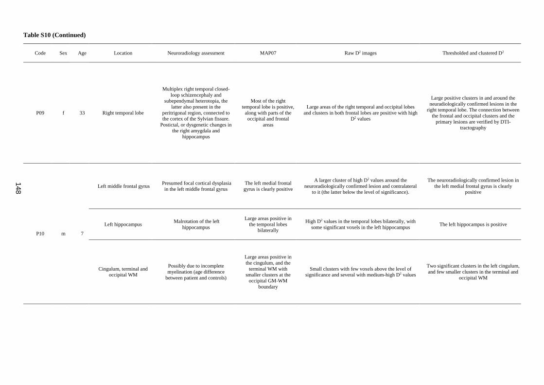
148

Table S10 (Continued)

Code Sex Age Location Neuroradiology assessment MAP07 Raw D2 images Thresholded and clustered D2

P09 f 33 Right temporal lobe

Multiplex right temporal closed-

loop schizencephaly and subependymal heterotopia, the

latter also present in the

peritrigonal region, connected to the cortex of the Sylvian fissure.

Postictal, or dysgenetic changes in

the right amygdala and hippocampus

Most of the right

temporal lobe is positive,

along with parts of the occipital and frontal

areas

Large areas of the right temporal and occipital lobes

and clusters in both frontal lobes are positive with high D2 values

Large positive clusters in and around the

neuradiologically confirmed lesions in the right temporal lobe. The connection between

the frontal and occipital clusters and the

primary lesions are verified by DTI-tractography

P10 m 7

Left middle frontal gyrus Presumed focal cortical dysplasia

in the left middle frontal gyrus

The left medial frontal

gyrus is clearly positive

A larger cluster of high D2 values around the

neuroradiologically confirmed lesion and contralateral to it (the latter below the level of significance).

The neuroradiologically confirmed lesion in

the left medial frontal gyrus is clearly positive

Left hippocampus Malrotation of the left

hippocampus

Large areas positive in

the temporal lobes bilaterally

High D2 values in the temporal lobes bilaterally, with

some significant voxels in the left hippocampus The left hippocampus is positive

Cingulum, terminal and occipital WM

Possibly due to incomplete

myelination (age difference

between patient and controls)

Large areas positive in

the cingulum, and the

terminal WM with smaller clusters at the

occipital GM-WM

boundary

Small clusters with few voxels above the level of significance and several with medium-high D2 values

Two significant clusters in the left cingulum,

and few smaller clusters in the terminal and

occipital WM

149

Table S10 (Continued)

Code Sex Age Location Neuroradiology assessment MAP07 Raw D2 images Thresholded and clustered D2

P11_S1 m 27

Basal region of the left

inferior frontal gyrus and

the posterior third of the left insula

Malformation of cortical development, presumably

polymicrogyria or FCD

Positive Medium-sized area with high D2 values in and around

the neuroradiologically confirmed lesion Positive

Left frontal, bilateral

occipital and temporal WM

No clear sign of abnormalities

Positivities in parts of

the left frontal, and bilateral temporal and

occipital lobes and in

most of the corona

radiata bilaterally

Several high D2 clusters, with some voxels above the

significance threshold

Clusters in the left frontal, the bilateral

occipital, and the left terminal WM, the latter is evidently connected to the primary

lesion, verified by DTI tractography.

Occipital registration artefacts are easy to

identify by their configuration

P11_S2 m 27

Basal region of the left

inferior frontal gyrus and

the posterior third of the

left insula

Malformation of cortical development, presumably

polymicrogyria or FCD

Positive Medium-sized area with high D2 values in and around

the neuroradiologically confirmed lesion Positive

Left frontal, bilateral

occipital and temporal

WM

No clear sign of abnormalities

Positivities in parts of

the left frontal, and

bilateral temporal and occipital lobes and in

most of the corona

radiata bilaterally

Several high D2 clusters, with some voxels above the

significance threshold. The right insula, contralateral to the neuroradiologically confirmed lesion contains

higher D2 values in a larger volume than previously

Most WM clusters further apart from the

neuroradiologically confirmed lesion are

still present. Fewer artefacts than previously

150

Table S10 (Continued)

Code Sex Age Location Neuroradiology assessment MAP07 Raw D2 images Thresholded and clustered D2

P12 m 14

Left hippocampus Left hippocampal sclerosis Negative Significantly high D2 values in the left hippocampus,

with high values in the surrounding WM Positive

Left temporal pole

Malformation of cortical

development (FCD-IIIa) in the left

temporal pole

Most of the left temporal lobe is marked positive

High D2 values in the WM of the left temporal pole, most voxels below the threshold of significance

One small positive cluster in the WM close to the left temporal pole

Right temporal pole Gliotic cyst with approx. 2mm size

in the right temporal pole

Most of the right

temporal lobe is marked

positive

Significantly high D2 values in the volume of the cyst, high D2 values in the surrounding tissue

Positive

WM in the posterior part

of the left and right superior frontal gyri

WM FLAIR signal alterations in

the right superior frontal gyrus

Clusters in the superior corona radiata are

marked positive

bilaterally

High D2 values in the superior frontal WM of both

hemispheres with right predominance

One cluster in either hemispheres in the

posterior parts of the superior frontal gyri

P13 m 35

Right temporal lobe

Right temporal closed-loop

schizencephaly and subependymal

heterotopia

Most of the temporal lobes and the superior

corona radiata are

marked positive bilaterally

The right temporal lobe contains the most voxels with

high D2-values clearly centered around the

neuroradiologically confirmed lesion

Large significant clusters in the right

temporal lobe and the hippocampus clearly

mark the pathology

Right occipital pole

Several WM signal alterations in

the occipital poles bilaterally with

right predominance. May be due to

circulatory disturbance(s) during

the 2nd trimester (the same cause may be behind the schizencephaly,

as well).

Positive, but with

smaller clusters and

weaker effect size

Frontal and occipital lobes contain regions of high D2 values bilaterally with right predominance

Several small clusters in the occipital lobes bilaterally with right predominance

Frontal lobes bilaterally

and the anterior part of

the right internal capsule

No clear sign of abnormalities

The frontal WM is

marked positive

bilaterally

Small clusters of higher D2-values with a few voxels above the level of significance

Few clusters in the frontal lobes and one in the anterior part of the right internal capsule

Results of independent lesion detection (MAP07) and the proposed Mahalanobis-distance based method were evaluated with the expert neuroradiologist (PB); apart from three cases, the

diagnoses of MCD subtypes were based on imaging.