Diffusion in Social and Information NetworksPart II

WORLD WIDE WEB2015, FLORENCE

MPI for Software Systems Georgia Institute of Technology

Le SongManuel Gomez Rodriguez

2

What is all about?

Stochastic processes over a

large networks

Modeling Information Diffusion

Modeling Social Activity

Basic Cascade ModelCascades as Point Processes

Beyond CascadesActivity as Hawkes Processes

PART I: MODELS

PART II: LEARNING METHODSInfluence Maximization

Submodular OptimizationScalable Algorithm

Source LocalizationMaximum likelihood

Estimation

Activity ShapingBeyond Influence Max

Convex Opt. Framework

3

Outline

Influence Maximization

Exact & Approx. EstimationApprox. Maximization

Source Localization Maximum likelihoodEstimation

Activity Shaping Beyond Influence MaxConvex Opt. Framework

4

Time-sensitive decision making

Can we seed information in a few sites, such that it can spread, in 1 month, to a million blogs?

Need to consider timing information

Need to be scalable

5

Influence of a set of sources

The influence is the average # of nodes infected up to time T by cascades that started in a set of sources nodes A. (icml’11)

# of nodes infected up to time T by a cascade that started in A

Probability of infection of node n given the source set A

Sink (node n)

SourcetA = 0tA = 0

tn

6

Maximizing the influence

Theorem. The continuous time influence maximization problem defined by Eq. (1) is NP-hard.

Once we know how to estimate influence, what about finding the set of source nodes that maximizes influence?

7

Submodularity of Influence Maximization

The influence function satisfies a natural diminishing property: submodularity!

if

The influence maximization can be reduced to a Set Cover problem

8

Submodular maximization

Theorem. The influence function is a submodular function in the set of nodes A.

Obtain a suboptimal solution with a 63% provable guarantee using the greedy algorithm:

9

Influence maximization vs. # of sources

1024-node Hierarchical Kronecker1024-node Forest Fire

512-node Random Kronecker 1000-node real network (MemeTracker)

10

Influence vs. time horizon

11

Influence estimation: exact vs. approx.

Sink (node n)

Source

tA = 0tA = 0

tn

ApproximateInfluence

Estimation

ExactInfection

Probability

Can be exponential in network size, not scalable!

12

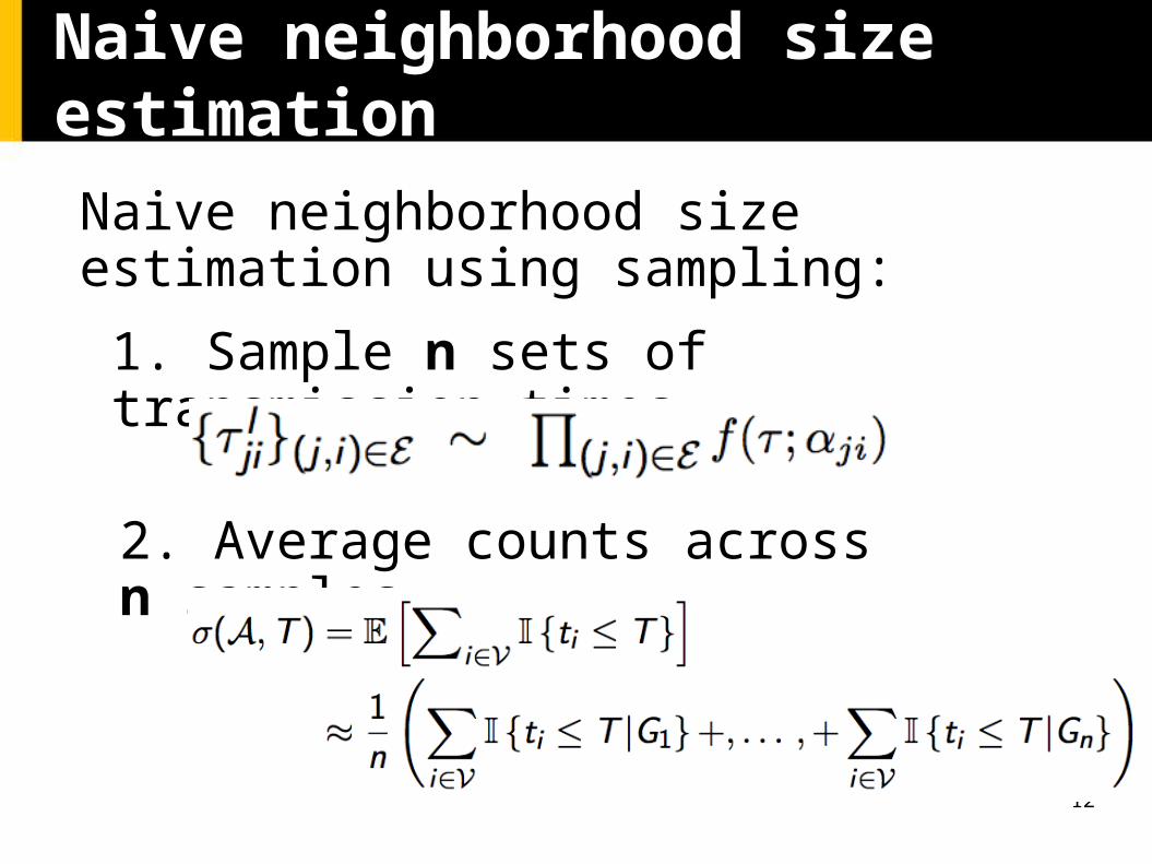
Naive neighborhood size estimation

Naive neighborhood size estimation using sampling:

1. Sample n sets of transmission times

2. Average counts across n samples

13

Naive neighborhood size estimation

Check whether length of shortest path is ≤TQuadratic in network

size (all pair of nodes), not scalable!

14

Neighborhood vs. P(ti ≤ T)

It is difficult to scale exact influence estimation to networks with million of nodes.

Key fact: No need to calculate each P(ti ≤ T) separately.

We only care about neighborhood!

15

Cohen’s neighborhood estimation

Key fact: Given a set of n i.i.d. random variables X ~ e-x, the minimum is distributed as X* ~ ne-nx

.

1. Draw m sets of i.i.d. random labels2. Find the minimum label at a distance ≤T by using Cohen’s algorithm.3. The neighborhood size is

The estimator is unbiased and with variance O(1/(m-2))

16

Cohen’s least label list

To find the minimum label at distance ≤T efficiently:

Increasing distance, decreasing label

Cohen [‘97] invented a smart algorithm to generate a label-list structure per node:

17

Multiple sources

Multiple sources:

18

How good is the approximation?

Not only theoretical guarantees, but it also works well in practice. Accuracy does not depend on the network structure

19

How scalable is the algorithm?

Small networks128 nodes, 320 edges

1 million nodes

Readily scale up to realistic networks with millions of nodes

20

Outline

Influence Maximization

Exact & Approx. EstimationApprox. Maximization

Source Localization Maximum likelihoodEstimation

Activity Shaping Beyond Influence MaxConvex Opt. Framework

21

Incomplete propagation traces

It is difficult to track every mention of a specific piece of information

Especially in real time!

Can we automatically find who was the first

person posting a piece of information?

22

The source identification problem

Information propagates on a directed network creating cascades:

We do not observed all infected nodes in a cascade, only a few of them.

Cascade 1

Source

Can we identify the source from the

network and a partial observation

of the cascade?

τji ~ f(τji ; αji)tj ti

23

Likelihood of a cascade

The likelihood of a cascade factorizes as

ts tk tl ti

Cascade

If we only observe a subset of infected nodes :

Marginalization over hidden nodes on

Time of infection of the source

Difficult high-dimensional integration problem

24

Framework for source identification

Infer diffusion model parameters from historical cascade data

Given the diffusion model & incomplete cascade (or cascades), identify the source:

STAGE 1

STAGE 2

Difficult high-dimensional integration problem

Non-convex maximization

25

Importance Sampling Scheme

First, we introduce auxiliary distribution:

Second, we introduce proposal distribution:

Auxiliary distribution

Proposal distribution

We will sample from this distribution!

It will simplify computations!

26

Choice of auxiliary & proposal distribution

Proposal distribution: sample from the diffusion model as if there were no observationswith node as source

Auxiliary distribution: sample from the diffusion model as if there were no observations with the hidden nodes as sources

27

Why those distributions?

1. We can sample easily from the proposal distribution and has good convergence properties in practice

2. The auxiliary distribution allows us to cancel out many terms

Likelihood of observed nodes

Likelihood ratio of hidden nodes with observed nodes as parents

Observed times

Sampled times

28

Maximize objective function

Key idea: each piece corresponds to a different feasible (temporally plausible) parent-child configuration:

Piece-wise continuous function on ts

1. We can find all change points efficiently

2. One dimensional line-search for each piece

2a. More efficiently for exponential transmission functions

29

Synthetic data experiments: setup

1. Generate network structure (Kronecker/Forest Fire)

2. Assign edge transmission rates uniformly at random

3. Simulate cascades from different random sources and record large cascades

4. Run our method to infer the source of large cascades from partial observations (typically, 10%)

30

A toy example

Hierarchical Kronecker Network (64 nodes)

As more cascades are observed, the likelihood of the true source beats other nodes’ likelihoods.

31

Success Probability vs Number of Cascades

Erdos-Renyi Random Network (256 nodes)Cascades longer than 40 nodes (10% observed)

Our method (blue) clearly beats competing methods

32

Success Probability vs Number of Cascades

Core-Periphery Kronecker Graph (256 nodes)Cascades longer than 40 nodes (10% observed)

difficult to distinguish among nodes in the core

33

Success Probability vs % Observed Infections

The more infections we observe, the easier it becomes

Core-Periphery Kronecker Graph (256 nodes)Cascades longer than 100 nodes

34

Success Probability vs Number of Samples

Hierarchical Kronecker Graph (256 nodes)Cascades longer than 40 nodes (10% observed)

Success probability flattens with the number of samples

35

Real data experiments: setup

1. Memes (“lipstick on a pig”) mentioned by 1,700 popular media sites & blogs for different topics [WSDM ‘13]

2. Infer diffusion network for each topic from memesusing a network inference method

3. We extract large (meme) cascades for each topic, here large means >27 nodes

4. Run our method to infer the source of large cascades from partial observations (typically, 10%)

36

Real Data: Success Probability vs Number of Cascades

Our method needs >7 cascades to (sometimes) find the sourceCompeting methods fail completely

Source identification in

real networks is a very

difficult problem!

37

Outline

Influence Maximization

Exact & Approx. EstimationApprox. Maximization

Source Localization Maximum likelihoodEstimation

Activity Shaping Beyond Influence MaxConvex Opt. Framework

38

Activity shaping

Can we steer users’ activity in a social network?

Why this goal?

Activity shaping… is this new?

Related to Influence Maximization Problem

39

One time the same piece of information

Fixed incentive

It is only about maximizing

adoption

Influence MaximizationActivityShaping

Variable incentive

Multiple times multiple pieces,

recurrent!

Many different activity shaping

tasks

Kempe et al. KDD’03 and many others

Influence maximization: simple but far from real social activity

Activity shaping: more challenging (at first)

but close to real social activity

Exogenous vs endogenous activity

Exogenous activityUsers’ actions due todrives external to thenetwork

Endogenous activityUsers’ responses to other users’ actions in the network

...

Activity shaping… how?

Incentivize a few users to produce a given

level of overall users’ activity

41Exogenous activity

Endogenous

activity

42

Endogenous & exogenous intensity

Exogenousactivity

Overall activity(events / day)

Endogenous activity

0.62 tweets/hour(13/11/2014)

0.54 tweets/hour(13/11/2014)

0.08 tweets/hour(13/11/2014)

... ...

43

Exogenous intensity: Hawkes

Influence of neighbor ui on user u

Previous event by a neighboor

Non-negative kernel (memory)

Endogenous activity

2:54 PM13 Nov

3:50 PM13 Nov

1:55 PM13 Nov

44

Activity shaping… what is it?

Activity Shaping: Find exogenous activity that results in a desired average overall activity at a given time:

Average with respect tothe history of events up to t!

45

Exogenous intensity & average overall intensity

How do they relate?

Surprisingly… linearly:

Convolution

matrix that depends on

influencematrix

non negativekernel

and

Exact Relation

46

Finally, if the kernel is exponential , then we can compute analytically:

Corollaryexogenous intensity

is constant

Matrixexponentials

Does it really work in practice?

47

48

Activity shaping optimization framework

Once we know that

we can find to satisfy many different goals:

ACTIVITY SHAPING PROBLEM Utility (Goal)

Cost for incentivizing

Budget

We can solve this problem efficiently

for a large family of utilities!

49

Capped activity maximization (CAM)

Max feasible activity per user

If our goal is maximizing the overall number of events across a social network:

50

Minimax activity shaping (MMASH)

If our goal is make the user with the minimum activity as active as possible:

51

Least-squares activity shaping (LSASH)

If our goal is to achieve a pre-specified level of activity for each user or group of users:

52

Solving the activity shaping problem

For any activity shaping problem, we need to:

Large matrixexponential

1. Compute:

2. Solve the convex problem:

Large matrixexponential

Inverse ofa large matrix

Standard: projected gradient descent

Can be cubic in the network size

1. [Al-Mohy et al., 2011]

53

Computing the average overall intensity

The explicit computation of becomes quickly intractable for large networks (large sparse A)

Key property: we don’t need but

2. Sparse linear systems of equations [GMRES method]:

54

URL shortenings in Twitter

Product for which we can track their users’ usage pattern in Twitter.

URL SHORTENING SERVICESbit.ly

tinyurl

is.gd

doiop

55

Evaluation of our model on real data

Two twitter networks with 2K users and 50K users who used URL shortenings over a 8 month period.

Fit model(s) on different time periods

Run many different activity shaping tasks

complex held-out evaluation

(close to intervention)

Evaluate theoretical & simulated results

vs baselines

56

Complex held-out evaluation

We divide the 8-month period into 50 contiguous 5-day sub periods:

Fit model andsolve activity

shaping

Fit model Fit model Fit model…

We sort distances (i) between exogeneous rates (ii) between overall activity

Compute rankcorrelation

…

57

Capped activity maximization: results

Theoretical Simulation Held-out evaluation

+10% more events than 2nd best

+34,000 more events per month than 2nd best

For 2K users:

58

Theoretical Simulation Held-out evaluation

Minimax activity shaping: results

For 2K users:

less active user 2x more events than 2nd best

less active user +4.32 more events per month than 2nd best

59

Least-square activity shaping: results

Theoretical Simulation Held-out evaluation

For 2K users:

We are always closer to target level than baselines.

60

Scalability of our algorithm

How does our efficient algorithm compare to a naive implementation of activity shaping?

Up to 10k users Up to 50k users

Our algorithm is several order of magnitude faster!

61

What is all about?

Stochastic processes over a

large networks

Modeling Information Diffusion

Modeling Social Activity

Basic Cascade ModelCascades as Point Processes

Beyond CascadesActivity as Hawkes Processes

PART I: MODELS

PART II: LEARNING METHODSInfluence Maximization

Submodular OptimizationScalable Algorithm

Source LocalizationMaximum likelihood

Estimation

Activity ShapingBeyond Influence Max

Convex Opt. Framework

62

Processes over networks

Economic Transactions

Disease Spread

Causes, Petitions & Non-Profit

63

Networks: tools and connections

Machine Learning & Data Mining

Event-History Analysis & Statistics

Computer Systems Theory &

Algorithms

Networks & Processes Over Networks

Social & Information Sciences

EconomicsDecisionTheory

Epidemiology

PhysicsBiology