Embed Size (px)
Citation preview

Dielectric response and partial dischargemeasurements on stator insulation
at varied low frequency
NATHANIEL TAYLOR
Doctoral ThesisStockholm, Sweden 2010

TRITA-EE 2010:037ISSN 1653-5146ISRN KTH/EE--10/037--SEISBN 978-91-7415-713-0
Elektroteknisk teori och konstruktionTeknikringen 33
SE-100 44 StockholmSWEDEN
Akademisk avhandling som med tillstand av Kungl Tekniska hogskolan framlaggestill offentlig granskning for avlaggande av teknologie doktorsexamen fredag den24 september 2010, klockan 10:00 i sal F3, Lindstedtsvagen 26, Kungl Tekniskahogskolan, Stockholm.
Nathaniel Taylor, August 2010.c©/ This thesis is placed in the public domain.
Tryck: Universitetsservice, US-AB

Abstract
This is a study of potential improvements of diagnostic methods used on high-voltage generators and motors. It considers offline electrical measurements onthe main insulation of stator windings, where a sinusoidal voltage is appliedbetween the winding and the stator-core, and the total current through theinsulation (dielectric spectroscopy, DS) and the rapid current-pulses arising fromdischarges (partial discharge, PD) are measured.
The proposed methods differ from existing practice in industrial DS andPD measurements in that the applied voltage is varied in amplitude and infrequency, harmonics of the voltage and current are measured, and the DS andPD measurements are made simultaneously, with comparison of results. Basedon literature, models and measurements, the problems and advantages of thesemethods are assessed in this work.
Harmonics provide a way of separating linear and nonlinear sources of cur-rent, and reveal the waveform of the current. Measurement of total PD chargeby DS methods provides complementary information to the conventional PDmeasurement; the difference in results between these types of measurementis shown by literature and experimental results to be large. Simultaneousmeasurement allows direct comparison of the relation between the DS andPD results, and saves time compared to separate measurements. The variedfrequency, down to the millihertz range, provides additional information aboutthe insulation. Much of the potential for DS methods on machine insulationis spoiled by the end-winding stress grading. Models and measurements of thecurrents in this grading are presented, with discussion of how much effect thedisturbance has and how well it can be predicted by modelling.

Chapters
1 Introduction 1
2 Stator insulation 9
3 Aging of insulation, natural and accelerated 23
4 Diagnostics and Prognostics 29
5 Dielectric Response 39
6 Dielectric Response measurement 55
7 Partial Discharges 73
8 Partial Discharge measurement 95
9 The Dielectric Spectroscopy instrument 105
10 The PD pulse-measurement instrument 115
11 Conjectured advantages of the new methods 123
12 Tests of the DS instrument 127
13 Tests of the PD instrument 137
14 Contribution of PD to the total DS current 151
15 Processing and display of DS and PD results 157
16 Effects of previous excitation on results 163
17 Comparison of DS and PD measurements 169
18 Stator coils used as test-objects 177
19 End-grading currents 183
20 SiC-based stress-grading material 201
21 Conclusions 213
A Principles 219
v


Contents
1 Introduction 1
1.1 Background . . . . . . . . . . . . . . . . . . . . . . . . . . . . . . 1
1.2 Aim . . . . . . . . . . . . . . . . . . . . . . . . . . . . . . . . . . 2
1.3 Main contributions . . . . . . . . . . . . . . . . . . . . . . . . . . 2
1.4 Reading guide . . . . . . . . . . . . . . . . . . . . . . . . . . . . . 3
1.5 Summary of work conducted . . . . . . . . . . . . . . . . . . . . 4
1.6 Scope and limitations of this work . . . . . . . . . . . . . . . . . 5
1.7 Comparison with initial aims . . . . . . . . . . . . . . . . . . . . 5
1.8 Conferences, publications and other external contact . . . . . . . 6
1.9 Notation and style . . . . . . . . . . . . . . . . . . . . . . . . . . 6
2 Stator insulation 9
2.1 Construction and materials . . . . . . . . . . . . . . . . . . . . . 92.1.1 Multiturn coils and Roebels bars . . . . . . . . . . . . . . 112.1.2 Insulation materials . . . . . . . . . . . . . . . . . . . . . 122.1.3 PD prevention at the surface . . . . . . . . . . . . . . . . 152.1.4 Assembly in the slots . . . . . . . . . . . . . . . . . . . . 162.1.5 Rotational speed . . . . . . . . . . . . . . . . . . . . . . . 172.1.6 Cooling . . . . . . . . . . . . . . . . . . . . . . . . . . . . 18
2.2 Failures in stator insulation . . . . . . . . . . . . . . . . . . . . . 192.2.1 Failures of rotating machines . . . . . . . . . . . . . . . . 192.2.2 Some stator insulation failure-modes . . . . . . . . . . . . 20
3 Aging of insulation, natural and accelerated 23
3.1 Insulation aging: mechanisms and synergies . . . . . . . . . . . . 23
3.2 Aging of stator insulation . . . . . . . . . . . . . . . . . . . . . . 233.2.1 Thermal aging . . . . . . . . . . . . . . . . . . . . . . . . 233.2.2 Thermal cycling . . . . . . . . . . . . . . . . . . . . . . . 243.2.3 Electrical aging . . . . . . . . . . . . . . . . . . . . . . . . 243.2.4 Ambient . . . . . . . . . . . . . . . . . . . . . . . . . . . . 263.2.5 Mechanical stress . . . . . . . . . . . . . . . . . . . . . . . 26
3.3 Accelerated aging . . . . . . . . . . . . . . . . . . . . . . . . . . . 26
4 Diagnostics and Prognostics 29
4.1 Diagnostic and prognostic aims . . . . . . . . . . . . . . . . . . . 29
4.2 Obtaining and interpreting data . . . . . . . . . . . . . . . . . . 30
4.3 Maintenance decisions . . . . . . . . . . . . . . . . . . . . . . . . 32
4.4 Establishing and updating rules . . . . . . . . . . . . . . . . . . . 32
vii
4.5 Measurements offline and online . . . . . . . . . . . . . . . . . . . 33
4.6 Cross-comparison, trending, and relative measures . . . . . . . . 35
4.7 Current practice for stator insulation . . . . . . . . . . . . . . . . 36
5 Dielectric Response 39
5.1 Basic electrical properties of materials . . . . . . . . . . . . . . . 39
5.2 Mechanisms and descriptions of dielectric response . . . . . . . . 41
5.3 Dielectric responses of materials . . . . . . . . . . . . . . . . . . . 44
5.4 Dielectric response of whole insulation systems . . . . . . . . . . 45
5.5 Dielectric response of stator insulation . . . . . . . . . . . . . . . 465.5.1 Mica, epoxy and asphalt . . . . . . . . . . . . . . . . . . . 465.5.2 The epoxy-mica or asphalt-mica composite . . . . . . . . 485.5.3 Currents in a healthy stator insulation system . . . . . . . 495.5.4 Chemical changes in the insulation . . . . . . . . . . . . . 505.5.5 Voids and insulation-expansion . . . . . . . . . . . . . . . 515.5.6 Electrostatic compression . . . . . . . . . . . . . . . . . . 525.5.7 Poor earthing of the bar surfaces . . . . . . . . . . . . . . 525.5.8 Water absorption . . . . . . . . . . . . . . . . . . . . . . . 535.5.9 Surface contamination . . . . . . . . . . . . . . . . . . . . 535.5.10 Fractures and pinholes . . . . . . . . . . . . . . . . . . . . 545.5.11 Summary . . . . . . . . . . . . . . . . . . . . . . . . . . . 54
6 Dielectric Response measurement 55
6.1 Dielectric-response measurements in time and frequency . . . . . 556.1.1 Time-domain measurements . . . . . . . . . . . . . . . . . 566.1.2 Frequency-domain measurements . . . . . . . . . . . . . . 57
6.2 Some practicalities of FDDS measurements . . . . . . . . . . . . 586.2.1 Input signals . . . . . . . . . . . . . . . . . . . . . . . . . 586.2.2 DFT components . . . . . . . . . . . . . . . . . . . . . . . 596.2.3 Distorted sources and nonlinear test-objects . . . . . . . . 626.2.4 Calculation of input current . . . . . . . . . . . . . . . . . 636.2.5 Error sensitivity . . . . . . . . . . . . . . . . . . . . . . . 646.2.6 Choice of feedback . . . . . . . . . . . . . . . . . . . . . . 656.2.7 Feedback ratio . . . . . . . . . . . . . . . . . . . . . . . . 66
6.3 DS measurements for general HV diagnostics . . . . . . . . . . . 68
6.4 DS measurements on stator insulation . . . . . . . . . . . . . . . 696.4.1 Capacitance and loss . . . . . . . . . . . . . . . . . . . . . 696.4.2 Insulation ‘resistance’ and polarisation index, IR/PI . . . 706.4.3 Less-common industrial methods . . . . . . . . . . . . . . 72
7 Partial Discharges 73
7.1 Gas discharges . . . . . . . . . . . . . . . . . . . . . . . . . . . . 737.1.1 Discharge and breakdown . . . . . . . . . . . . . . . . . . 737.1.2 Paschen’s law . . . . . . . . . . . . . . . . . . . . . . . . . 747.1.3 Electron avalanches . . . . . . . . . . . . . . . . . . . . . 74
viii

7.1.4 Starting-electrons . . . . . . . . . . . . . . . . . . . . . . . 757.1.5 Continued supply of electrons . . . . . . . . . . . . . . . . 767.1.6 The Townsend breakdown mechanism . . . . . . . . . . . 767.1.7 The streamer breakdown mechanism . . . . . . . . . . . . 77
7.2 Partial Discharge origins . . . . . . . . . . . . . . . . . . . . . . . 797.2.1 Classification of sources . . . . . . . . . . . . . . . . . . . 797.2.2 Features of coronas . . . . . . . . . . . . . . . . . . . . . . 807.2.3 Features of cavity PD . . . . . . . . . . . . . . . . . . . . 817.2.4 Forms of discharge in PD . . . . . . . . . . . . . . . . . . 83
7.3 Frequency-dependence of PD . . . . . . . . . . . . . . . . . . . . 857.3.1 Frequencies already of practical interest . . . . . . . . . . 857.3.2 Varied frequency for greater information . . . . . . . . . . 867.3.3 Causes of frequency-dependence . . . . . . . . . . . . . . 87
7.4 Discharge forms of PD in epoxy and stator insulation . . . . . . 88
7.5 PD sources in stator insulation systems . . . . . . . . . . . . . . 89
8 Partial Discharge measurement 95
8.1 PD detection and measurement in general . . . . . . . . . . . . . 95
8.2 Apparent-charge measurement . . . . . . . . . . . . . . . . . . . 968.2.1 From site to electrodes . . . . . . . . . . . . . . . . . . . . 968.2.2 From electrodes to terminals . . . . . . . . . . . . . . . . 988.2.3 The external circuit and detection . . . . . . . . . . . . . 988.2.4 Display of results . . . . . . . . . . . . . . . . . . . . . . . 100
8.3 Non-pulse measurement of apparent-charge . . . . . . . . . . . . 101
8.4 Difficulties of PD measurement in stator windings . . . . . . . . 1018.4.1 Repetition rate . . . . . . . . . . . . . . . . . . . . . . . . 1018.4.2 Noise and dynamic range . . . . . . . . . . . . . . . . . . 1028.4.3 PD-pulse propagation . . . . . . . . . . . . . . . . . . . . 102
8.5 Current practice in stator-PD measurement . . . . . . . . . . . . 104
9 The Dielectric Spectroscopy instrument 105
9.1 Description of the IDAX300 and HVU . . . . . . . . . . . . . . . 1059.1.1 Voltage synthesis . . . . . . . . . . . . . . . . . . . . . . . 1069.1.2 The HVU . . . . . . . . . . . . . . . . . . . . . . . . . . . 1079.1.3 Voltage measurement . . . . . . . . . . . . . . . . . . . . 1089.1.4 Specimen earthing . . . . . . . . . . . . . . . . . . . . . . 1089.1.5 Electrometers and feedback . . . . . . . . . . . . . . . . . 1099.1.6 ADCs and digital processing . . . . . . . . . . . . . . . . 1109.1.7 Calibration . . . . . . . . . . . . . . . . . . . . . . . . . . 111
9.2 Computer control . . . . . . . . . . . . . . . . . . . . . . . . . . . 112
9.3 Automatic selection of feedback-component values . . . . . . . . 113
9.4 Alternative types of instrument . . . . . . . . . . . . . . . . . . . 114
ix

10 The PD pulse-measurement instrument 115
10.1 Description of the ICM components . . . . . . . . . . . . . . . . 11510.1.1 Preamplifier . . . . . . . . . . . . . . . . . . . . . . . . . . 11610.1.2 Main amplifier . . . . . . . . . . . . . . . . . . . . . . . . 11610.1.3 Digitiser . . . . . . . . . . . . . . . . . . . . . . . . . . . . 11710.1.4 Synchroniser and PD memory . . . . . . . . . . . . . . . . 11810.1.5 Gate . . . . . . . . . . . . . . . . . . . . . . . . . . . . . . 11910.1.6 Controller . . . . . . . . . . . . . . . . . . . . . . . . . . . 11910.1.7 Calibrator . . . . . . . . . . . . . . . . . . . . . . . . . . . 119
10.2 Computer control . . . . . . . . . . . . . . . . . . . . . . . . . . . 120
10.3 Alternative types of instrument . . . . . . . . . . . . . . . . . . . 120
11 Conjectured advantages of the new methods 123
11.1 Differences from conventional measurements . . . . . . . . . . . . 123
11.2 Evolution of the aim . . . . . . . . . . . . . . . . . . . . . . . . . 124
11.3 Matters for investigation . . . . . . . . . . . . . . . . . . . . . . . 126
12 Tests of the DS instrument 127
12.1 Correctness of calculation of voltage and current . . . . . . . . . 127
12.2 Output voltage starting and stopping phase . . . . . . . . . . . . 128
12.3 Steps in output voltage . . . . . . . . . . . . . . . . . . . . . . . 128
12.4 Interference frequency . . . . . . . . . . . . . . . . . . . . . . . . 128
12.5 Variation of results with feedback-component . . . . . . . . . . . 130
12.6 Consistency between measurements . . . . . . . . . . . . . . . . . 131
12.7 Output voltage phase-shift and offset . . . . . . . . . . . . . . . . 134
13 Tests of the PD instrument 137
13.1 Phase-shift . . . . . . . . . . . . . . . . . . . . . . . . . . . . . . 137
13.2 PDP compression . . . . . . . . . . . . . . . . . . . . . . . . . . . 137
13.3 PDP transfer times . . . . . . . . . . . . . . . . . . . . . . . . . . 138
13.4 PDP transfers while running . . . . . . . . . . . . . . . . . . . . 139
13.5 ADC characteristics . . . . . . . . . . . . . . . . . . . . . . . . . 140
13.6 Synchronisation . . . . . . . . . . . . . . . . . . . . . . . . . . . . 142
13.7 Linearity . . . . . . . . . . . . . . . . . . . . . . . . . . . . . . . . 144
13.8 Calibrator pulses . . . . . . . . . . . . . . . . . . . . . . . . . . . 147
13.9 Signal limits . . . . . . . . . . . . . . . . . . . . . . . . . . . . . . 148
14 Contribution of PD to the total DS current 151
14.1 Comparison of DS and PD results . . . . . . . . . . . . . . . . . 151
14.2 Measurement of pulsed currents . . . . . . . . . . . . . . . . . . . 151
14.3 Summary . . . . . . . . . . . . . . . . . . . . . . . . . . . . . . . 155
x

15 Processing and display of DS and PD results 157
15.1 Conventional measurements and presentation . . . . . . . . . . . 157
15.2 Further data from the proposed measurements . . . . . . . . . . 157
15.3 Suggested presentation . . . . . . . . . . . . . . . . . . . . . . . . 15815.3.1 PD patterns . . . . . . . . . . . . . . . . . . . . . . . . . . 15815.3.2 DS including harmonics . . . . . . . . . . . . . . . . . . . 159
16 Effects of previous excitation on results 163
16.1 Physical-system properties of stator insulation . . . . . . . . . . . 163
16.2 Standard measurement practice . . . . . . . . . . . . . . . . . . . 164
16.3 Varied amplitude and frequency . . . . . . . . . . . . . . . . . . . 16516.3.1 Example of effects of recent excitation on PD . . . . . . . 166
16.4 Recommendation for swept measurements . . . . . . . . . . . . . 167
17 Comparison of DS and PD measurements 169
17.1 DS and PD on laboratory objects . . . . . . . . . . . . . . . . . . 16917.1.1 Point-hemisphere . . . . . . . . . . . . . . . . . . . . . . . 17017.1.2 Cavity object . . . . . . . . . . . . . . . . . . . . . . . . . 17117.1.3 A single stator-coil . . . . . . . . . . . . . . . . . . . . . . 173
17.2 Full stator-windings . . . . . . . . . . . . . . . . . . . . . . . . . 174
18 Stator coils used as test-objects 177
18.1 Construction . . . . . . . . . . . . . . . . . . . . . . . . . . . . . 177
18.2 Heating . . . . . . . . . . . . . . . . . . . . . . . . . . . . . . . . 179
18.3 DS measurements on the guarded slot-part . . . . . . . . . . . . 180
19 End-grading currents 183
19.1 Stress-grading methods . . . . . . . . . . . . . . . . . . . . . . . 183
19.2 Cylindrical laboratory-models on PTFE . . . . . . . . . . . . . . 184
19.3 Spectroscopy Results . . . . . . . . . . . . . . . . . . . . . . . . . 18519.3.1 Fundamental-frequency components of current . . . . . . 18519.3.2 Harmonic currents . . . . . . . . . . . . . . . . . . . . . . 186
19.4 Numerical Models . . . . . . . . . . . . . . . . . . . . . . . . . . 18719.4.1 Linear, discrete . . . . . . . . . . . . . . . . . . . . . . . . 18719.4.2 Linear, distributed . . . . . . . . . . . . . . . . . . . . . . 18819.4.3 Nonlinear, discrete . . . . . . . . . . . . . . . . . . . . . . 19019.4.4 Nonlinear, distributed . . . . . . . . . . . . . . . . . . . . 19119.4.5 Discussion of model results . . . . . . . . . . . . . . . . . 193
19.5 Measurements on real stator insulation . . . . . . . . . . . . . . . 19519.5.1 Dielectric response of end-windings alone . . . . . . . . . 19519.5.2 Dielectric response of entire bars . . . . . . . . . . . . . . 198
xi

20 SiC-based stress-grading material 201
20.1 Literature on the material properties . . . . . . . . . . . . . . . . 20120.1.1 Models of electrical properties . . . . . . . . . . . . . . . . 20120.1.2 Complications: further parameters and variation . . . . . 202
20.2 Material measurements on PTFE tubes . . . . . . . . . . . . . . 20320.2.1 Temperature-dependence of the SiC material . . . . . . . 20520.2.2 Electrode contact with SiC material . . . . . . . . . . . . 207
20.3 Material measurements on real stator insulation . . . . . . . . . . 20720.3.1 Measurements with dc . . . . . . . . . . . . . . . . . . . . 20920.3.2 Measurements with ac . . . . . . . . . . . . . . . . . . . . 210
20.4 Summary . . . . . . . . . . . . . . . . . . . . . . . . . . . . . . . 212
21 Conclusions 213
21.1 Main results . . . . . . . . . . . . . . . . . . . . . . . . . . . . . . 21321.1.1 PD measurement by DS . . . . . . . . . . . . . . . . . . . 21321.1.2 PD charge by DS or PD-pulse . . . . . . . . . . . . . . . . 21321.1.3 Stress-grading response . . . . . . . . . . . . . . . . . . . 21321.1.4 Frequency-dependence of PD . . . . . . . . . . . . . . . . 213
21.2 Suggestions for future investigation . . . . . . . . . . . . . . . . . 21421.2.1 Frequency-dependence . . . . . . . . . . . . . . . . . . . . 21421.2.2 Simultaneous DS and PD on whole windings . . . . . . . 21421.2.3 Parameter estimation for end-grading models . . . . . . . 21421.2.4 Study of service-aged bars . . . . . . . . . . . . . . . . . . 21521.2.5 Ignoring or estimating the fundamental current . . . . . . 21521.2.6 Time-sequence, and non-sinusoidal excitation . . . . . . . 215
A Principles 219
A.1 Precision of expression . . . . . . . . . . . . . . . . . . . . . . . . 219A.1.1 Numbers . . . . . . . . . . . . . . . . . . . . . . . . . . . 219A.1.2 Equations . . . . . . . . . . . . . . . . . . . . . . . . . . . 220A.1.3 Sensitivity . . . . . . . . . . . . . . . . . . . . . . . . . . . 220A.1.4 Examples . . . . . . . . . . . . . . . . . . . . . . . . . . . 220A.1.5 Graphical presentation . . . . . . . . . . . . . . . . . . . . 220
A.2 Comparison of ‘research methods’ . . . . . . . . . . . . . . . . . . 222A.2.1 Aims . . . . . . . . . . . . . . . . . . . . . . . . . . . . . . 222A.2.2 Disturbances . . . . . . . . . . . . . . . . . . . . . . . . . 223A.2.3 Classes of subject-area . . . . . . . . . . . . . . . . . . . . 224A.2.4 Classification of this work . . . . . . . . . . . . . . . . . . 226A.2.5 Formal methods of analysis . . . . . . . . . . . . . . . . . 227A.2.6 Experimental design . . . . . . . . . . . . . . . . . . . . . 230A.2.7 Presentation of results . . . . . . . . . . . . . . . . . . . . 234A.2.8 Aggregation and comparison . . . . . . . . . . . . . . . . 235
A.3 Working practices . . . . . . . . . . . . . . . . . . . . . . . . . . 236A.3.1 Preparation . . . . . . . . . . . . . . . . . . . . . . . . . . 236A.3.2 Notes and data . . . . . . . . . . . . . . . . . . . . . . . . 236
xii

A.3.3 Control-programs . . . . . . . . . . . . . . . . . . . . . . . 237A.3.4 Processing of results . . . . . . . . . . . . . . . . . . . . . 238
A.4 Computers and programs . . . . . . . . . . . . . . . . . . . . . . 239A.4.1 Awareness of the possibilities . . . . . . . . . . . . . . . . 239A.4.2 Toolchains and cooperation . . . . . . . . . . . . . . . . . 240A.4.3 Speeding things up . . . . . . . . . . . . . . . . . . . . . . 242A.4.4 Numerical versus Analytical . . . . . . . . . . . . . . . . . 243A.4.5 Numerical inidealities . . . . . . . . . . . . . . . . . . . . 244
xiii


List of Tables
9.1 IDAX300 feedback component values . . . . . . . . . . . . . . . . . . 110
13.1 Approximate times for PDP transfers . . . . . . . . . . . . . . . . . . 13913.2 The ICM commands for setting ADC characteristics . . . . . . . . . . 141
20.1 Grading-material parameters on different substrates . . . . . . . . . . 20320.2 Material-parameters fitting measurements on SiC materials . . . . . . 205
xv


List of Figures
2.1 Basic construction of stator core . . . . . . . . . . . . . . . . . . . . . 92.2 Stator core and winding of a several-megawatt motor . . . . . . . . . 102.3 Diagrams of multiturn coil and Roebel bar. . . . . . . . . . . . . . . . 112.4 Cross-sections of stator windings in their slots. . . . . . . . . . . . . . 17
4.1 The generalised diagnostic/prognostic process . . . . . . . . . . . . . 30
5.1 Cross-sections of lapped tapes and mica flakes . . . . . . . . . . . . . 485.2 Sources of DR current in stator insulation . . . . . . . . . . . . . . . . 50
6.1 Contributions of various time-functions to 1st harmonic . . . . . . . . 616.2 Electrometer feedback circuit for analysis of input current . . . . . . . 646.3 Electrometer feedback circuit for analysis of voltage offsets . . . . . . 676.4 Examples of C-tan δ tip-up results from real stators . . . . . . . . . . 71
7.1 A crude classification of PD sources . . . . . . . . . . . . . . . . . . . 797.2 Some parameters determining frequency-dependence of cavity PD . . 877.3 Sources of PD in stator insulation . . . . . . . . . . . . . . . . . . . . 907.4 Some classic PD-pattern shapes for stator PD . . . . . . . . . . . . . 91
8.1 PD dipole affecting the electrodes . . . . . . . . . . . . . . . . . . . . 978.2 PD apparent-charge measurement . . . . . . . . . . . . . . . . . . . . 998.3 Signals at the input and output of PD preamplifier . . . . . . . . . . 100
9.1 Picture of the IDAX300 DS-instrument and its HVU . . . . . . . . . 1059.2 Diagram of the IDAX DS-instrument’s typical use . . . . . . . . . . . 1069.3 Diagram of the IDAX DS-instrument’s components and signals . . . . 107
10.1 Picture of the ICM PD-instrument . . . . . . . . . . . . . . . . . . . . 11510.2 Diagram of the ICM PD-instrument’s components . . . . . . . . . . . 11610.3 Diagram of the ICM PD-instrument’s components and signals . . . . 118
12.1 Smoothness of IDAX output voltage even at low amplitude . . . . . . 12912.2 Mains interference when measuring open-circuit . . . . . . . . . . . . 12912.3 Variation of results with choice of feedback components . . . . . . . . 13112.4 C′ and C′′ measured on a gas capacitor . . . . . . . . . . . . . . . . . 13212.5 Automatic feedback settings for amplitude and frequency sweep . . . 13312.6 Capacitance with sweeps up and down in frequency . . . . . . . . . . 13312.7 Phase-shifts between IDAX applied voltage and TTL output . . . . . 134
13.1 Variation of ICM’s recorded phase with frequency . . . . . . . . . . . 13813.2 Reading the ICM’s PDP during running acquisition . . . . . . . . . . 14013.3 ADC characteristics and quantisation levels . . . . . . . . . . . . . . . 14113.4 Testing conversion of charge-channel to charge. . . . . . . . . . . . . . 14213.5 ICM synchronisation for different commands . . . . . . . . . . . . . . 143
xvii

13.6 ICM synchronisation for varied phase of triggering . . . . . . . . . . . 14413.7 ICM main-amplifier output +/− ratios, on PDP . . . . . . . . . . . . 14513.8 ICM main-amplifier output +/− ratios, on oscilloscope . . . . . . . . 14613.9 Differences in measured + and − magnitude . . . . . . . . . . . . . . 14613.10 Series capacitor (ac-coupling) improving ICM +/− ratio . . . . . . . 14713.11 Calibrator pulse waveforms and spectra . . . . . . . . . . . . . . . . . 14813.12 ICM amplifier output signal limits . . . . . . . . . . . . . . . . . . . . 149
14.1 Pulses of constant charge and varied phase . . . . . . . . . . . . . . . 15314.2 Pulses of constant charge and varied pulse-width . . . . . . . . . . . . 15314.3 Pulses of varied charge and phase, measured with varied feedback . . 15414.4 Harmonics corresponding to figure 14.3 . . . . . . . . . . . . . . . . . 15414.5 Time-domain currents from IDAX for sharp pulses . . . . . . . . . . . 155
16.1 PR-PDP with varied off-time since last excitation . . . . . . . . . . . 16616.2 PD current with varied off-time since last excitation . . . . . . . . . . 167
17.1 PD test-objects: point-hemisphere, cavity, stator coil . . . . . . . . . 16917.2 PDP for the point-hemisphere object . . . . . . . . . . . . . . . . . . 17017.3 Measurements of PD currents for the point-hemisphere object . . . . 17117.4 PDP for the cavity object . . . . . . . . . . . . . . . . . . . . . . . . . 17217.5 Measurements of PD currents for the cavity object . . . . . . . . . . . 17217.6 Stator-coil PD current from DS and PD systems . . . . . . . . . . . . 17317.7 Stator-coil PD currents at varied frequency . . . . . . . . . . . . . . . 17417.8 Raw PDP measured for slot PD . . . . . . . . . . . . . . . . . . . . . 17517.9 PDP for slot PD . . . . . . . . . . . . . . . . . . . . . . . . . . . . . . 17517.10 PDP for a ‘normal’ stator winding . . . . . . . . . . . . . . . . . . . . 17617.11 Mean currents due to the PDPs . . . . . . . . . . . . . . . . . . . . . 176
18.1 Picture of all six stator-bars . . . . . . . . . . . . . . . . . . . . . . . 17718.2 Constructional details of the new coil-halves . . . . . . . . . . . . . . 17818.3 The large laboratory-oven for thermal aging . . . . . . . . . . . . . . 17918.4 Fundamental-frequency capacitance for slot-part . . . . . . . . . . . . 18018.5 Capacitance of slot-part after removal of C∞ . . . . . . . . . . . . . . 18118.6 Voltage-dependence of slot-part capacitance . . . . . . . . . . . . . . . 18218.7 Capacitance for slot-part after postcure . . . . . . . . . . . . . . . . . 182
19.1 Field around a truncated electrode without grading . . . . . . . . . . 18319.2 Diagram of simple laboratory models of stress-grading . . . . . . . . . 18419.3 Picture of graded PTFE tubes using paint and tape . . . . . . . . . . 18519.4 Capacitance and loss measured for bar5 (taped). . . . . . . . . . . . . 18619.5 C′ & C′′ for 1D grading: linear/nonlinear, discrete/distributed . . . . 18819.6 Components of 1D grading model . . . . . . . . . . . . . . . . . . . . 19119.7 Results from nonlinear distributed 1D model . . . . . . . . . . . . . . 19219.8 Comparison measurement with 1D nonlinear distributed model . . . . 19319.9 Fundamental-frequency capacitance of end-gradings . . . . . . . . . . 19619.10 Pure end-grading capacitances of guarded bar . . . . . . . . . . . . . 19619.11 Subtraction of constant or frequency-dependent capacitance . . . . . 19719.12 Measured odd-harmonic magnitudes in current . . . . . . . . . . . . . 19819.13 Full bar, ∆C′ and C′′ . . . . . . . . . . . . . . . . . . . . . . . . . . . 19919.14 Capacitance and loss of stator bar with and without guarding . . . . 199
xviii

19.15 Relative magnitudes of current-harmonics in slot and ends . . . . . . 20019.16 Total C′ and C′′ for four different . . . . . . . . . . . . . . . . . . . . 200
20.1 Samples of SiC paint and tape on PTFE tubes . . . . . . . . . . . . . 20420.2 Measurement of dc I/V for samples on PTFE tubes . . . . . . . . . . 20520.3 Data for SiC powder, fitted with curves . . . . . . . . . . . . . . . . . 20620.4 Temperature-dependence of grading material dc I/V relation . . . . . 20620.5 Contact-dependence with electrode on pre-cured tape surface . . . . . 20720.6 Samples of VPI-treated SiC tape on a real stator bar . . . . . . . . . 20820.7 I/E relations with dc, for SiC grading on real bars . . . . . . . . . . . 20920.8 Complex-capacitance view of grading material sample . . . . . . . . . 21020.9 Quasi-dc I/V (0.1 Hz) for grading material . . . . . . . . . . . . . . . 211
xix

Acknowledgements
I am very thankful for the opportunity I have had to study in this broadand deep area of high-voltage insulation. This work has been carried out withinElektra project 36019, financed jointly by the Swedish Energy Agency, Elforsk,ABB and Banverket.
Hans Edin has been the most directly involved supervisor in this work,from the formulation of the proposal through to this, the culmination, givingencouragement and help throughout and coping admirably with my frequentapplication of ‘just-in-time management’. This work in some parts continueshis PhD [Edi01], considering its possible application to stator insulation.
Roland Eriksson introduced me to this subject during my exchange year in2001, and later offered me the PhD position. To hear again such physicsy wordsas ‘electron’, after having been away for nearly two years working in the area ofpower-systems, was most refreshing. The smooth running of the division duringthis time, including the easy availability of whatever resources have been neededin the laboratory and computer rooms, has been much appreciated.
Rajeev Thottappillil moved here from Uppsala as the new professor onRoland’s retirement, and therefore ended up adopting the project at aboutthe time when the original plans would have suggested it to be finishing (thediscrepancy being due to earlier parental leave). I’ve appreciated our chatsabout electromagnetics, and the instructive course in EMC that he gave longbefore we knew that we would later be in the same department.
Sven Jansson has faithfully represented Elektra at all of the half-yearly‘reference group’ meetings for the project, keeping us in touch with relatedprojects and industrial interest.
Eva Martensson of ABB Motors helped with advice at the project meetings,and with providing specimens for the tests of real stator bars and materials.Hans-Ake Eriksson was Eva’s predecessor, and provided other stator coils andhelp in my first years here.
Tommy Karlsson of Vattenfall Power Consultant gave useful advice at ourmeetings, also organising some field-measurements about half-way through thisproject and providing extra data to help me get a better idea of typical generator-parameters and results from conventional diagnostic measurements. Within thesame company, Kristoffer Backstrom helped by providing data from measure-ments on whole stators.
Ingvar Hagman, while at STRI, very helpfully and efficiently organised accessto some generators for field-measurements. I deeply regret that I have not (yet)been able to take advantage of these, owing to the long delays in having all theparts of the measurement system in working order and then the more pressingneed of finishing the laboratory work.
Cecilia Forssen was the first ‘room sharer’, patiently enduring my practicein spoken Swedish. Our later discussions of PDs, measurement methods andexperimental design helped my knowledge and enthusiasm. Valentinas Dubickasstarted at the same time as I did, and we shared a room in his last year here. His
xx

help with my few forays into high-frequency work, and general discussions atstarting-work time, were well appreciated. Nadja Javerberg then moved in, andwe have had shared interest in dielectric measurements, battles against certaininstruments, and welcome tea-breaks from all of this. Mohamad Ghaffarian andXiaolei Wang, who recently joined the research group, have already awakenedmy interest in their projects. Lars Jonsson of the electromagnetic theory groupwithin our department has brought stimulation to some afternoons by visits todiscuss ways of doing all manner of things with computers, and has done muchto encourage communication between the diverse research-groups in our seminarseries.
Valerijs Knazkins was in the power systems department, upstairs, evenbefore my arrival at KTH. A wealth of shared interests, and my liking for slightlykeeping up on the work of other divisions, have made for many enjoyable lunches,fikas, and small-hours email exchanges. Katherine Elkington started workingupstairs a few years ago, and has similarly brightened the scene of lunches,tea-breaks and extra-departmental technical discussions. Dmitry Svechkarenko,from the machines department along the corridor, has been a regular lunch-taker and a contact with yet another department’s work, and his company andtable-tennis playing are eagerly requested by my children if we pass by ‘the workplace’ at the weekend.
Peter Lonn, the computer administrator for our building, has been mosthelpful in obtaining many parts and programs and organising purchases for allmy activities with lab computers, file servers and computation servers.
Many people around the world have done the work of writing and polishingthe computer programs that have made some parts of this work a pleasure,rather than the agony of most of the alternative offerings. The GNU utilities,TEX, Perl, Octave, KDE, Linux, the Gentoo build-system and FreeBSD, alongwith countless other programs, were of immense value on our computers in thelab, on the desktop, in the server room and on the move. Thank you Stallman,Knuth, Torvalds, Lamport, Eaton, Wall, and countless others.
My family — Malin, Nicholas, Philip and William — have suffered sporadicperiods of over-activity around particular equipment-troubles or deadlines, andhave been particularly helpful in these last months. I hope the benefits of thisflexibly timetabled job have not been too heavily outweighed by these downsides!
xxi


Chapter 1
Introduction
1.1 Background
Stator insulation is a critical part of the high-voltage rotating machines thatare used as generators to produce practically all electrical power, and as largemotors to consume some of this power in driving industrial processes.
The high capital-costs of high-voltage machines themselves, and the usuallyhigh costs arising from a machine being unavailable for service, result the use of‘diagnostic’ measurements. These are typically applied at regular maintenanceintervals, with the intention of predicting failures and thereby avoiding them bysuitable maintenance.
Many types of diagnostic measurement are in widespread use on statorinsulation, yet the complexity of the insulation and of the aging and failureprocesses make each method just a further indication of insulation condition:there is nothing that reliably gives warning if and only if there is a real problem,and certainly nothing that gives accurate predictions of how long the insulationwill tolerate given stresses without failure.
The diagnostic methods can be improved by any combination of increasingthe likelihood of identifying an important problem, reducing the likelihood ofmissing an important problem, or reducing the time taken for measurements,or reducing the capital cost of equipment used for these measurements.
The methods investigated here are an extension and combination of two ofthe many types of measurement used to assess the condition of stator insulationfor the purpose of guiding decisions about operation and maintenance. Dielectricspectroscopy (DS) measures all the current that flows between electrodes of aninsulation system in response to a voltage stimulus. Partial discharge (PD)pulse measurement measures sharply pulsed components in the current due tobreakdown of small volumes of gas that are exposed to a strong electric fieldwithin an insulation system.
1

2 Chapter 1: Introduction
1.2 Aim
The aim of the project is to investigate a combined system for frequency-domainDS and phase-resolved PD measurements, and its application to diagnosticmeasurements on stator insulation. The DS and PD methods are extended inways beyond the current practice: the harmonic components in the DS currentare studied to help distinguish different sources and see the shape of the currentwaveform; the simultaneous use of the DS and PD measurements permits twocomplementary measurements of the charge due to PD, which increases theavailable information; a variable frequency is used, down to values much lowerthan in operation, permitting distinctions to be made between different typesof defect that could give similar results at the single frequency that is currentpractice. Several ideas have been pursued for these extensions of establishedmethods could be applied in diagnostic measurements on stator insulation.Investigations have been made based on literature, laboratory studies, field dataand simulation.
1.3 Main contributions
The following are the main new results in this thesis.Measurement of PD charge waveforms has been compared between the two
types of measurement, DS and PD, for several types of test object, showingsimilar measurement of PD charge in simple objects, and strong differences inlarger objects. The differences mean that the two types of measurement givecomplementary results for stator windings.
Tests of instruments and measurements have been made, to assess the prac-ticality of measuring PD currents with the DS instrument, to establish howto make the instruments work together, and to show that the results of sweptdiagnostic measurements can depend strongly on details of sequence and timing.
A review of stator insulation and diagnostic methods is given in the earlychapters, focused on points relevant to the proposed methods. It is based onbooks, old and recent research papers, laboratory measurements and resultsof industrial diagnostic measurements. Its usefulness is in providing detailsthat are needed for evaluating the usefulness of the proposed methods, forexample the relative sizes of signals and disturbances, and the relative influenceof different defects on lifetime.
The current in end-winding stress-grading have been measured on simpleobjects and on real stator bars, and numerical models have been made. Thedetailed appearance of this current, showing capacitance, loss and harmonicsas functions of voltage amplitude and frequency, has not been found elsewhere,yet it is important for understanding the influence on DS measurements andpossibly reducing this influence by modelling.
Characterisation of stress-grading materials was necessary for the modelling.Several simple materials models have been used in previous work, with littlejustification or detail about the range of applicability. Results are presentedfrom measurements over wide ranges of electric field and low frequency, withcomparison of the fit of mathematical models from the literature.

1.4 Reading guide 3
1.4 Reading guide
The table of contents is the probably the best starting place for a reader withvery limited time, followed by chapter 11 if wanting to get an overview.
Chapters 2 to 8 give background information about stator insulation, faultsin stator insulation, general diagnostic methods, and the phenomena and mea-surements associated with the DS and PD methods studied here. The start-ing level may seem rather basic, but there are many points of relevance towhether the proposed types of measurement might have a benefit. Each ofthese background chapters covers a subject that could easily fill a book, so theyare necessarily biased towards the matters relevant to stator insulation.
Chapters 9 and 10 describe the instruments, and chapters 12 and 13 describesome tests that were made on them: these are all quite detailed, and may be ofinterest to the reader who wishes to understand the potentials and limitationsof the measurements, or who uses these instruments.
Chapter 11 brings together the project description with details from theprevious chapters, to give a description of which of the many possible uses ofthe proposed measurements seem most promising.
Chapters 14 and subsequent chapters, up to the conclusion in chapter 21,investigate the questions raised in chapter 11, for example the phase-resolvedmeasurement of total PD charge, the display of DS and PD data measured atmany points, and disturbances due to currents in the end-windings.
The Appendix is an anomaly, detouring into such subjects as working-practices, computers, and attitudes to experiment and scientific inference.
* * *
I hope the quite long, dense structure of this thesis is not too off-putting topotential readers. It is partly due to the unusually broad scope of the project,studying two broad types of measurement, each extended to an extra controlledvariable, and with their relation also being considered. Part of the work isassessment of the possibilities, so there is not just a single tightly-defined threadto follow. Diagnostic methods, particularly in stator insulation, involve manypossible types of defect, differing in their criticality and in the extent of overlapor difference that they show in results of measurements.
I know only too well how most people who read a thesis will be interested onlyin extracting a few results, quickly. I, too, have seldom felt able to justify thetime needed to read a whole thesis in detail, even when of only some fifty lightlyfilled pages. For some reason, I wanted to make a thorough compilation of themain ingredients of the project. Quite how long this would take was not remotelyrealised at the start of writing: had more time been available, there would havebeen much more careful shortening, checking and honing, pulling together of thedifferent threads of the work, and more thorough cross-referencing and indexing.Nevertheless, I hope the current structure, along with the contents and index,makes it fairly easy for readers to skip to the particular details in which theyare interested, in spite of the large range of subjects included.
4 Chapter 1: Introduction
1.5 Summary of work conducted
Literature studies have been made on several key subjects: stator insulationsystems, aging of stator insulation, accelerated-aging testing, diagnostic meth-ods, dielectric response of materials and stator insulation systems, PD in statorinsulation, methods and limitations of PD detection, and PD signal transmissionin stator windings. Some of the main results are included in the early chapters.
Stress-grading material made for stator end-windings has been characterisedfor use in the models of end-winding currents. Measurements in the lab havestudied conductivity and permittivity and their dependence on the amplitudeand frequency of the applied electric field. The literature has been searched formodels and measurements on these types of materials, to get an idea of howvariable the parameters are likely to be in different machines.
Currents in end-windings flowing in stress-grading systems have been stud-ied by laboratory models, several levels of numerical models, and measurementson real stator bars. The frequency-domain representation of this current, includ-ing low-order harmonics, has been studied as a function of the applied voltage’samplitude and frequency.
Measurement systems for DS and PD measurements have been acquiredas two commercially available instruments, and programs have been writtento control them in ways more versatile than their provided programs, partlyto facilitate the later combined measurements; a lot of work was taken indetermining how to control the instruments and make them work together.Together with an external amplifier the DS instrument can apply voltages atamplitudes up to 20 kV and frequencies from 100µHz to above 100Hz.
Simultaneous measurement with both of the measurement systems requiredsome modifications compared to separate measurements, due to the signal-earthing arrangements and to the problem of electrical noise from the HV sourceaffecting the PD measurement.
PD charge-measurements have been compared between PD-pulse measure-ments and measurement of the whole current by DS methods. Reasons forthe differences between DS and PD measurements of PD charge have beeninvestigated, by a study of literature on PD detection and calibration, someanalysis, and some laboratory work.
Presentation of measurement-results is particularly important given the largenumber of controlled and measured variables compared with conventional diag-nostic methods. Suitable ways of presenting results have been considered, andprograms have been written to implement them. Suggestions have been madeof apparently useful indices of insulation condition.
Dependence on voltage and frequency of the currents in various features anddefects of stator insulation have been considered, based on literature, simplemodels and measurements.
Thermal aging in the laboratory has been made possible by building an ovenlarge enough for several bars to fit in, and able to be heated to 200 C.
Stator coils received in new condition have been used for measurements ofmaterial properties and of currents in the end-windings, before and after slowheating to finish curing the insulation.

1.6 Scope and limitations of this work 5
1.6 Scope and limitations of this work
The measurements considered here require a sinusoidal voltage of controlledamplitude and frequency to be applied to the terminals of entire isolated sectionsof stator-winding. The neutral-point of the winding must be able to be isolatedfrom earth, and preferably split to separate the phases. This makes these meth-ods inherently ‘offline’, requiring some work in preparing for the measurement,but still more convenient than methods that require direct access to parts deepinside the machine. The main insulation is stressed between the equipotentialsof the conductor and the earthed core of the machine; the insulation betweenturns in a multiturn coil is therefore not directly tested. The mica-based form-wound type of insulation that is assumed here is used at rated voltages of about1 kV and above. The end-winding stress grading that has been studied in thiswork is used above about 5 kV: this range is the main focus here, but some ofthe work is also relevant to rather lower rated voltages.
This work is deliberately limited to the diagnostic purpose of relating resultsof measurements to the probable state of the insulation that has given theseresults. Even this, in view of the many possible types of defect in statorinsulation and the uncertainties involved in distinguishing them, is a quitevague and difficult subject. The further important steps, of deciding the futureoperation and maintenance in order to optimise the use of the machine, arelargely ignored for the sake of limiting the scope. There is however somedistinction made between defects known to give very fast or very slow failure,when discussing the potential of the new types of measurement.
1.7 Comparison with initial aims
The initial project-proposal suggested several paths that have been followedand several that have not. The measured dielectric response current due toPD was to be investigated: this has indeed been a large part of the work.The role of end-winding stress grading systems in obscuring the results of DSmeasurements has taken a prominent place in the work; the initial interest inthis grading was as a possible source of PD when at low frequencies, but thisturned out to be unimportant. Simultaneous measurement of DS and PD wasmentioned, just with respect to ‘on-site’ (field) measurements: simultaneousmeasurement has been an important part of the work, but has not yet beenapplied to whole stator windings on-site. Variable-frequency phase-resolvedPD analysis (VF-PRPDA) was to be used: it has been, but there has not beentime for a systematic experimental investigation of PD frequency-dependence ofvarious common types of stator PD-source. Other proposals were more towardsdoing analyses on naturally aged insulation from old machines by the electricalmethods, comparing results with dissection and chemical analysis: there hasinstead been work with laboratory objects and artificial aging. Investigationof the economic benefits of these methods for maintenance was to be studied:this has been avoided for the reasons explained in section 1.6. On the otherhand, extensive consideration mainly based on literature has been given to theimportance of identifying particular types of defect.

6 Chapter 1: Introduction
1.8 Conferences, publications and other external contact
Papers have been presented at some conferences, giving the opportunity ofmeeting people with an academic and industrial interest in this work. These con-ferences and papers were CEIDP 2004 [Tay04], ISH 2005 [Tay05], NordIS 2007[Tay07] and NordIS 2009 [Tay09]. Similar events that were attended withoutpresenting work were NordIS 2005 in Trondheim, the International Symposiumon Electrical Insulation ISEI 2006 in Toronto, and the European ElectricalInsulation Manufacturers’ seminar EEIM 2005 in Berlin.
A paper about stress-grading models has been accepted for a rotating-machines special issue of the IEEE Transactions on Dielectrics and ElectricalInsulation, due later this year. Papers on several other subjects started in thisthesis are hoped to be submitted to reviewed journals in the near future.
A licentiate thesis [Tay06] was published at the half-way point of this projectin November 2006. The main parts are either covered in more detail here or arereferred to when needed.
Several industrial contacts have resulted in useful exchanges of information,and opportunities for studying or fabricating real stator insulation. Contactswith these companies have been maintained through the half-yearly meetingsabout this project, and by some intermediate visits to discuss results. In col-laboration with Vattenfall Power Consultant, measurements have been made ona hydro-generator before and after some maintenance work; DS measurementswere performed as well as the standard set of measurements, as has already beendescribed in [Tay06]. Vattenfall has also provided some results from routinemeasurements on various sizes of hydro-generator, which have been used to getan idea of the range of typical values. ABB Motors has provided two batchesof new epoxy-mica stator coils: the first batch was studied in [Tay06], and thesecond batch has been partially studied here, including a specially fabricatedcoil with many material-samples. ABB Corporate Research gave use of its ovensfor the earlier thermal aging, before a large enough oven was constructed in thelaboratory at KTH. Contact with STRI has made some generators available formeasurements, but the opportunity has not yet arisen to carry out this work.
1.9 Notation and style
Emphasis is shown by italic type, and technical terms being defined are indicatedby slanted type. Names and abbreviations are explained in the most relevantchapter, not necessarily where they first appear; the index on page 247 shouldallow the definitions to be found. Symbols are defined close to their first use.
Having been expected to write in English, I have followed my preference ofhaving notational conventions match the language conventions. Examples arethe use of the letter V to denote voltage, a dot as the decimal separator, andthe ‘cross’ symbol for multiplication; these are usual in English and are usedin many countries outside Europe, but not in most other European languages,including Swedish. The modern sense of ‘data’ as a singular word describing‘stuff’ is used without the slightest compunction when it seems natural; so, too,is the plural sense . . . .

1.9 Notation and style 7
Quantities that are functions of time are generally lower-case, for examplei(t), and their frequency-domain transforms are upper-case, I(ω). Phasor quan-tities, represented as complex numbers, are so common that no special bar orboldness is used to emphasise their vectorial nature. Subscripts denoting namesare roman, iin, and subscripts denoting variables are italic, in. Some specialmathematical symbols are indicated by roman type: i is the imaginary unit, ethe base of natural logarithms, and d the differential operator.
The widely varying magnitudes of physical quantities can be expressed usingSI prefixes, for example 530 pC, or by using standard-index notation with non-prefixed units, for example 5.30×10⁻¹⁰ C. The prefix method has been chosenhere. For quantities in the limited exponent-range needed for most of this workit is rather shorter, and it permits many discussions to stick to a simple rangeof ones to thousands of some unit such as picocoulombs; its disadvantage is thatone cannot see whether, for example, the zero in ‘530 pC’ is a significant digit.
The units of quantities presented in plots and tables are shown in brackets,for example Q [pC], which is concise and unambiguous for all the needs in thiswork. The method recommended by standards organisations, of writing thequantity together with its conversion into a ‘pure number’, for example Q/pC,is indeed more versatile for some complex cases, but is arguably less concisewhen divisions are desired within quantities such as i/v or units such as V/mm,which prompts an ugly proliferation of grouping-parentheses or a recourse toexponents such as V·(mm)−1. Prefixes are used consistently, and are chosen tofit the subject: for example, kV/mm and mm/µs seem more appropriate thanthe base quantities or other prefixes when dealing with PD in cavities.
Equations are referred to by just their number in parentheses. Some ‘empir-ical’ equations are included, using a convenient function to describe a relationto an acceptable accuracy within some range; examples are (7.1) and (20.1).In contrast to derived equations, the empirical equations may be dimensionallyinconsistent; explicit division of each variable by its unit has not been used, sothe variables should be treated as being already pure numbers. This conventionis common in the engineering subjects in which such equations are used.
Cross-references mostly use a compact notation of sections or pages in brack-ets: this sentence is in [s.1.9] on [p.7]. Citations of papers and books use theauthor-year format, taking the first three letters of the first author’s surnamethen the last two digits of the year, and appending a letter if disambiguationis needed: this thesis could be [Tay10]. Citations of standards-documents usea single letter to denote the organisation, followed by the standard-number.Compared to the simple numbering that seems the commonest method in en-gineering, this takes rather more space and can be a little ugly, but it is muchclearer and more memorable: a reader familiar with the field would be able toguess many of the sources at a glance. The bibliography is right at the end tomake it easy to flick over to it for looking up citations whenever this does becomenecessary. If a freely available electronic version of a document is known of, alink to it is included in the bibliography entry. References to particular parts oflong works include a page, section or chapter number within the citation, suchas [Tay10, p.7]. Only one citation or cross-reference is ever used within a pair

8 Chapter 1: Introduction
of brackets.

Chapter 2
Stator insulation
This chapter describes the components of a stator, variations between machinesof different power and speed ratings, commonly used insulation systems, andsome common types of defect and fault. Diagnostic methods used on statorinsulation are described later, in chapter 4. The focus here is mainly on detailsthat are needed in the later chapters. For a broader and deeper treatment ofrotating-machine insulation in the stator, rotor and core, over a wide range ofages and power ratings, [Sto04] is highly recommended. Some papers givinggood descriptions of stator insulation materials are [Bou04] and [McD93].
2.1 Construction and materials
The stator of an ac rotating machine (motor or generator) is a stationaryconstruction consisting of a core of laminated steel that carries the magneticfields, surrounding structures that support this core, and windings of insulatedconductors that carry currents to produce the stator’s magnetic field. A simplediagram of a stator core is shown in figure 2.1, as a cross-section that indicatesthe shape of each thin (< 1mm) steel lamination, and as a three-dimensionalview showing the length.
axis
tooth
slot
length
back
stator core
borerotor
Figure 2.1: Basic construction of the stator core. To the left is a cross-section, indicatinghow a single lamination would look. There would typically be many more slots and teeth.Details of the rotor are not shown.
The steel of the core is an electrical steel, suitable for carrying alternatingmagnetic flux without high power losses. Such steel is often referred to asthe iron of the machine. It is an alloy of iron with some percent of silicon, alittle aluminium, and possibly some copper; several other elements, in particularcarbon, have to be excluded as much as possible in order to get good magneticproperties. The laminations have thin insulation on their surfaces to preventthe large circulating currents that would otherwise be induced by the magneticflux passing through the core.
Each lamination has pieces punched out to form the central bore in whichthe rotor is placed. Around the bore, slots are punched out, with teeth left
9

10 Chapter 2: Stator insulation
between the slots to carry the magnetic flux that links with the rotor. Radiallybeyond the teeth and slots is the back, which links the teeth together to carrythe magnetic flux between the groups of slots forming different magnetic poles.There are radial gaps forming cooling ducts at regular intervals along the axiallength of the core to allow cooling air or other gas to circulate.
The winding occupies the slots, and extends beyond the core in the end-winding (or overhang) region, where each insulated conductor emerges from itsslot and travels tangentially some way around the end of the core before passinginto another slot or connecting to a terminal.
Figure 2.2 shows end-views of a large motor whose rotor has been removedto expose the inside of the stator core. The bore is about 1m in diameter.
Figure 2.2: The stator core and winding of a several-megawatt motor, with the rotor removed.
In the left picture some of the supporting structure outside the core can beseen. In the centre picture and the close-up on the right, the stator slots can beseen running axially, the cooling ducts that carry radial air-flows can be seenrunning tangentially, along the face of the stator iron on the inside surface ofthe bore. The winding can only be seen at the end-winding parts, as the slotparts are covered by the wedges that hold the winding in place. In the rightpicture the supports within the end-winding can be seen.
Although these images give a useful impression of the main features of theconstruction of high-voltage stator windings, it should be borne in mind thatthere is much variation in the size and appearance between different machines.
The electrical connection of windings is very varied between machines. It canbe expected that there will be three phases, usually with one side of each phase-winding connected to a star-point (neutral). In a small machine each phase-winding may simply consist of a single piece of copper, a conductor, passingback and forth through the slots between the neutral and high-voltage terminals.In a large machine a phase-winding may consist of several such conductors atdifferent positions around the stator, connected in parallel to thick ring-busesthat run around the end-windings; each of these conductors may in turn consistof several parallel strands (also known as subconductors) running adjacent, tocope with the high currents.
2.1.1 Multiturn coils and Roebels bars 11
2.1.1 Multiturn coils and Roebels bars
Low-voltage generators and motors, with rms line-voltage† not more than about1 kV, have random-wound stators in which a thinly insulated wire is insertedin the slots without particular attention to the relative placement of the manyadjacent wires; the insulation is mainly determined by mechanical requirements.This type of machine is not considered at all in this work.
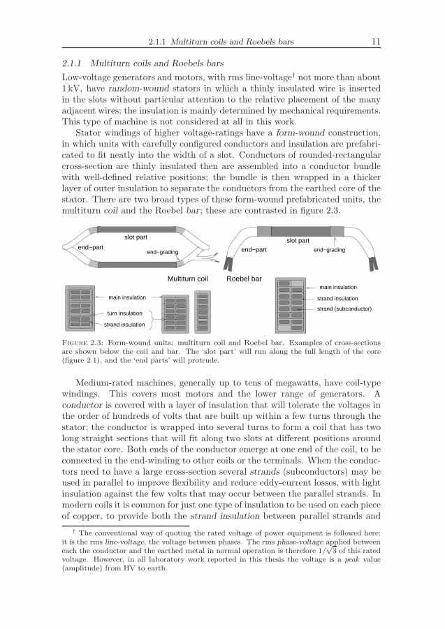
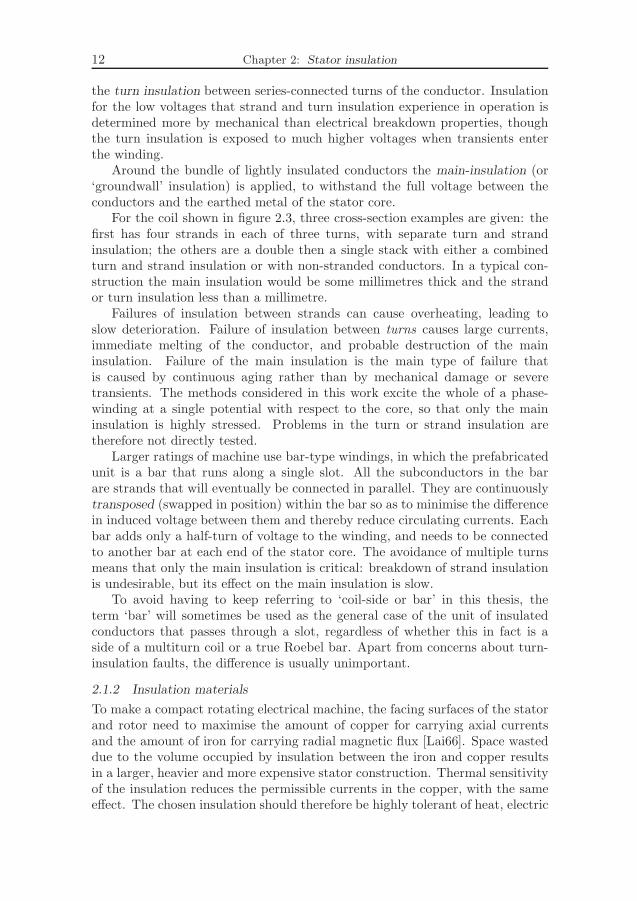
Stator windings of higher voltage-ratings have a form-wound construction,in which units with carefully configured conductors and insulation are prefabri-cated to fit neatly into the width of a slot. Conductors of rounded-rectangularcross-section are thinly insulated then are assembled into a conductor bundlewith well-defined relative positions; the bundle is then wrapped in a thickerlayer of outer insulation to separate the conductors from the earthed core of thestator. There are two broad types of these form-wound prefabricated units, themultiturn coil and the Roebel bar; these are contrasted in figure 2.3.
end−grading end−gradingend−partslot partslot part
end−part
Roebel barMultiturn coil
main insulation
strand insulation
turn insulation
strand insulation
strand (subconductor)
main insulation
Figure 2.3: Form-wound units: multiturn coil and Roebel bar. Examples of cross-sectionsare shown below the coil and bar. The ‘slot part’ will run along the full length of the core(figure 2.1), and the ‘end parts’ will protrude.
Medium-rated machines, generally up to tens of megawatts, have coil-typewindings. This covers most motors and the lower range of generators. Aconductor is covered with a layer of insulation that will tolerate the voltages inthe order of hundreds of volts that are built up within a few turns through thestator; the conductor is wrapped into several turns to form a coil that has twolong straight sections that will fit along two slots at different positions aroundthe stator core. Both ends of the conductor emerge at one end of the coil, to beconnected in the end-winding to other coils or the terminals. When the conduc-tors need to have a large cross-section several strands (subconductors) may beused in parallel to improve flexibility and reduce eddy-current losses, with lightinsulation against the few volts that may occur between the parallel strands. Inmodern coils it is common for just one type of insulation to be used on each pieceof copper, to provide both the strand insulation between parallel strands and
† The conventional way of quoting the rated voltage of power equipment is followed here:it is the rms line-voltage, the voltage between phases. The rms phase-voltage applied betweeneach the conductor and the earthed metal in normal operation is therefore 1/
√3 of this rated
voltage. However, in all laboratory work reported in this thesis the voltage is a peak value(amplitude) from HV to earth.
12 Chapter 2: Stator insulation
the turn insulation between series-connected turns of the conductor. Insulationfor the low voltages that strand and turn insulation experience in operation isdetermined more by mechanical than electrical breakdown properties, thoughthe turn insulation is exposed to much higher voltages when transients enterthe winding.
Around the bundle of lightly insulated conductors the main-insulation (or‘groundwall’ insulation) is applied, to withstand the full voltage between theconductors and the earthed metal of the stator core.
For the coil shown in figure 2.3, three cross-section examples are given: thefirst has four strands in each of three turns, with separate turn and strandinsulation; the others are a double then a single stack with either a combinedturn and strand insulation or with non-stranded conductors. In a typical con-struction the main insulation would be some millimetres thick and the strandor turn insulation less than a millimetre.
Failures of insulation between strands can cause overheating, leading toslow deterioration. Failure of insulation between turns causes large currents,immediate melting of the conductor, and probable destruction of the maininsulation. Failure of the main insulation is the main type of failure thatis caused by continuous aging rather than by mechanical damage or severetransients. The methods considered in this work excite the whole of a phase-winding at a single potential with respect to the core, so that only the maininsulation is highly stressed. Problems in the turn or strand insulation aretherefore not directly tested.
Larger ratings of machine use bar-type windings, in which the prefabricatedunit is a bar that runs along a single slot. All the subconductors in the barare strands that will eventually be connected in parallel. They are continuouslytransposed (swapped in position) within the bar so as to minimise the differencein induced voltage between them and thereby reduce circulating currents. Eachbar adds only a half-turn of voltage to the winding, and needs to be connectedto another bar at each end of the stator core. The avoidance of multiple turnsmeans that only the main insulation is critical: breakdown of strand insulationis undesirable, but its effect on the main insulation is slow.
To avoid having to keep referring to ‘coil-side or bar’ in this thesis, theterm ‘bar’ will sometimes be used as the general case of the unit of insulatedconductors that passes through a slot, regardless of whether this in fact is aside of a multiturn coil or a true Roebel bar. Apart from concerns about turn-insulation faults, the difference is usually unimportant.
2.1.2 Insulation materials
To make a compact rotating electrical machine, the facing surfaces of the statorand rotor need to maximise the amount of copper for carrying axial currentsand the amount of iron for carrying radial magnetic flux [Lai66]. Space wasteddue to the volume occupied by insulation between the iron and copper resultsin a larger, heavier and more expensive stator construction. Thermal sensitivityof the insulation reduces the permissible currents in the copper, with the sameeffect. The chosen insulation should therefore be highly tolerant of heat, electric
2.1.2 Insulation materials 13
stress and the discharges that may occur in any small gaps that may arise withinthe insulation.
The natural mineral mica is strongly resistant to damage by thermal, chem-ical and electrical mechanisms, and for this reason has provided the electricalstrength in main-insulation of high-voltage machines for about a century. Anorganic impregnant is used to fill the spaces between the pieces of mica, and togive greater mechanical strength and heat transfer. This composite insulation isunique to the special demands of rotating machines, contrasting with the waxedand oiled papers common in transformers, bushings† and power cables, or thesynthetic polymers of more modern power cables.
Mica is a laminar structure of highly chemically-inert flakes. There areseveral forms, differing a little in chemical structure and physical properties.The muscovite form is used in machine insulation. It can operate up to about550 C [Sto04, p.83], well beyond the capability of any impregnant that is used.
Up until the 1940s the mica for main insulation was in the form of splittings,layers split from sheets of natural mica. These were mounted on a backing of anatural-polymeric substance such as Kraft paper, and bonded with the naturalresin shellac, forming micafolium sheets. The development of mica-paper in the1940s was first driven by scarcity of large pieces of mica for making micafolium.Small pieces of mica are broken into very small pieces, then a paper-makingprocess is used to produce a thin layer on a backing material such as fibresof glass or synthetic polymer. It was soon found that although there is morefree-space in the mica paper compared to micafolium, a thorough pressing andremoval of surplus impregnant can increase the density of mica, and combinedwith the much more consistent thickness of mica paper the final product isactually better. In the decades following the introduction of mica paper, somestators were insulated with micafolium, some with mica paper, and some witha combination of the two [Eva81]. An approximate cross-section of insulationbuilt from mica paper is shown in figure 5.1 [p.48]. Modern production processesuse machines to wind the tape with more consistent position and tightness thanis achieved by hand; later parts, in particular around connections in the end-winding, are taped by hand. In spite of being applied by machine, tapes appliedin normal production facilities are found sometimes to have defects of gaps andwrinkles [Vog06] in a newly manufactured winding.
Mica in the forms described above would provide very little mechanicalstrength and would contain voids all over where discharges could happen. Thespaces are filled with an impregnant compound that holds the flakes together,filling whatever gaps remain. Again, the period from 1940 to the early 1950swas a time of large change. The impregnant used up to this time was anasphalt, sometimes called an asphaltic-resin or bitumen. This is a thermoplasticmaterial, meaning that it softens at increased temperature. The asphalt canmigrate out of some parts of the insulation when at high temperature. Thehigh chance of spaces being left in the insulation due to migration of asphaltlimited the service stress to about 2 kV/mm. The asphalt and the varnishes
†Bushing: an insulating structure around a high-voltage conductor, to allow it to passthrough a surface at another potential, typically earth.
14 Chapter 2: Stator insulation
applied between layers of micafolium sometimes had drying-oils included, togive less softening of the insulation with temperature; operating temperatureswould generally be above the glass-transition temperature, so the insulation wasstill soft even if not readily flowing. The effect of oxidation by long exposure athigh temperature in air also helps to harden the asphalt, but this will not happenin hydrogen-cooled machines. Asphaltic insulation expands considerably withtemperature, making a much tighter fit of bars in slots when at operatingtemperature rather than cold. The asphalt-micafolium type of insulation hasa high dielectric loss compared to later insulation, and has a non-negligibleconductivity. It also absorbs water, causing an increased dielectric loss andcapacitance. Asphalt-micafolium insulation is usually of temperature class†
130, which implies a normal operating temperature some tens of celsius lowerthan this number. In the early 1940s polyester-resin started to be used asa replacement for asphalts. This is a thermoset material that is cured afterimpregnation, to become a stable solid. It has the advantages of not meltingeven at high temperature, having higher mechanical strength, and being muchless absorbant of water. In the late 1940s epoxy-resin started to be used.Epoxides have all the functional advantages of polyesters, along with even bettermechanical strength and thermal stability; they also shrink far less on curing.The main troubles were the cost and the high viscosity of impregnant, whichrequired incorporation in the mica tapes since it would not easily flow intothe insulation from outside. The viscosity was soon improved, and the cost isapparently considered worthwhile in modern stator insulation, which in high-voltage machines almost always uses epoxy-resin. The resultant composite ofmica, glass-fibre and epoxy resin is mechanically strong, with a tensile strengthrather greater than that of copper [Tav08, p.14]. Electrical stresses are typically3 kV/mm, and can be as much as 5 kV/mm [Sto04, p.75]. The thinner insulationpermitted by the thermoset materials leads to greater thermal conductance outof the windings, and more space available for copper. The thermosets alsopermit higher operating-temperatures, epoxy-mica being usually of class F,155 C. All of these factors increase the potential rating or compactness ofa machine. The transition from asphalts to epoxy-resin did not of coursehappen as a sharp step: asphaltic systems continued to be used for somedecades after the introduction of the synthetic resins. A standard [E43, p.17]for testing ‘insulation resistance’ [s.6.4.2] assumes that post-1970 insulation willbe synthetic.
There are three main ways of getting the impregnant into the assembledmica-based insulation. Vacuum-pressure impregnation, VPI, was used even onearly asphaltic systems and is still in wide use. The insulation is dried and putin a chamber where it is exposed to a very low pressure, to get air and dampnessout. The chamber is then flooded with impregnant, and the pressure is drivenup to several atmospheres to force the impregnant into the insulation. Excessimpregnant is cleaned off, and the modern systems are then heated to cure
† The insulation temperature-classes are either a number or (deprecated) a letter. Thenumber is the temperature, in degrees Celsius, expected to give a 20 000 hour lifetime bysome definition of thermal degradation [Sto04, p.57]. Common in stator insulation are classes155 (F) and 130 (B). The actual operation is usually well below this value.

2.1.3 PD prevention at the surface 15
them, a typical treatment being 160 C for two hours. VPI can be categorisedas having two variations, global and individual. In global VPI the coils orbars are inserted in their slots in the core, with connections made and end-winding supports assembled, then this entire stator assembly is put into theVPI process. This has the advantage of not requiring already-hardened coils tohave to be forced into their slots; it also creates a firm bond and good heat-transfer between the coils and the slots. It is the method commonly used formachines rated in the tens of megawatts, which includes most large motors. Inindividual VPI of coils or bars, these components are put through the VPI andcuring processes and then are inserted in the stator. Although global VPI hasbeen used on increasingly large machines, up to some 200MW on some recentturbo-generators [Sto04, p.143], the larger sizes all use individually processedbars or coils, with the further advantage that each one can be inspected andelectrically tested before being accepted for insertion in the stator. The non-VPImethod is resin-rich insulation, where the impregnant is combined in the micatapes, and the bars or coils are then cured by hot-pressing to force the layerstogether at the curing temperature. This was originally used when epoxy-resincompounds were too viscose to impregnate the windings from outside, but it isstill the preferred method by some manufacturers.
The turn and strand insulation will not be covered in detail here, as onlythe main insulation is stressed in the types of measurement used in this work.Traditional turn-insulation is like thin main-insulation, and modern combinedstrand/turn insulation sometimes uses specially durable synthetic polymers to-gether with thin mica paper.
2.1.3 PD prevention at the surface
Small gaps are inevitable between a bar and the stator core, or between adjacentbars connected to different phases. In stators of some 5 kV rating and higher,these gaps could have high enough electric field to cause PD if they were notshielded. A mildly conductive coating called the slot semiconductor or slotcorona-protection is applied around the outside of the main insulation, in theform of varnishes painted onto the bars or tapes wrapped outside the tapedinsulation. The material must conduct enough to prevent PD, but not so muchas to cause considerable loss by currents driven by the induced voltage alongthe length of the slot. Carbon-black is a filler commonly used to provide theconductivity. The surface resistivity† to achieve this ranges from about 100Ω upto 2 kΩ [Eme96] or 10 kΩ [Sto04, p.24]. It is quite variable, depending on batchvariations, the layer’s applied thickness, and manufacturing treatments such asimpregnation; it is also affected by aging, which can reduce the resistivity byseveral times [Eme96] over the insulation’s lifetime.
† Surface-resistivity: the resistance between opposite sides of any square slab of the surface:this depends on material (bulk) resistivity and surface thickness, and is independent of thesize of the square. It is a useful description for situations where the current runs along alayer whose thickness as well as material are fixed. The unit is Ω as opposed to Ωm for bulkconductivity, and is sometimes written ‘Ω/sq’ to emphasise that it is a general property ofany square of the surface, not the resistance of a particular object.
16 Chapter 2: Stator insulation
As the windings emerge into the end-winding region, another type of semi-conductive coating may be applied, extending some ten centimetres along thebars to limit the surface electric field around the end of the slot-semiconductor.This is explained in more detail in chapter 19. It is referred to in this work as theend-winding stress-grading ; among its other names are end corona protectionand end semiconductor. It is common in windings rated above about 5 kV,and is increasingly adopted at voltages down to about 3.3 kV [Sto04, p.158] onmachines that are to be used with IFDs [s.7.3.1]. The material has stronglynonlinear conductivity [s.20.3]: the surface resistivity of the coating is a fewgigohms at quite high fields around 300V/mm, and increases some orders ofmagnitude at low fields. The end-winding region beyond this region has nosurrounding conductor or semiconductor, so capacitive coupling exists betweenthe end-windings.
Within a Roebel bar a soft semiconducting layer may also be put aroundthe whole group of strands, providing an equipotential layer between the lightlyinsulated strands and the main insulation, to prevent PD in voids between therounded strands and the wound main-insulation tape.
It is common for the entire end-winding part of a coil to be covered with atop layer of insulating material, even covering the stress-grading. This providessome protection against chemical and mechanical damage, but makes assessmentand repair of the stress-grading more difficult.
For very high-voltage stators a mildly conductive layer may be applied on thesurfaces of the end-windings; this is thought to help in passing a ‘hipot’ test.The surface resisitivity of hundreds of kilohms quoted in [Sto04, p.26] makesthis closer to slot semiconductor than to the end-winding grading; presumablyit results in a surface at a high and substantially uniform potential, separatedfrom the slot semiconductor by the usual stress-grading.
2.1.4 Assembly in the slots
The bars or coils are inserted in the slots, usually with two bars or coil-halvesstacked radially in each slot. In figure 2.4 cross-sections are shown of coil-sidesand bars in their slots. Note that some of the strands in the bar-type windinghave ducts for direct water-cooling, as described in section 2.1.6.
A slot wedge of insulating material runs in grooves along the open end ofeach slot to hold the bars in place. It is very important to hold the bars tight inthe slot, even after the changes in the insulation that occur from curing, agingand exposure to electromagnetic forces. Vibration can mechanically abradethe outer surfaces of the bars. In machines of some 20MW and above it iscommon to have a two-part wedge with some degree of elasticity, to maintainsome force even if the bars slightly shrink [Sto04, p.27]. The need of elasticityin the wedging is greater in thermoset insulation [McD93]; the insulation hasnot the thermoplastic materials’ tendency to fill extra space, and the hard edgesof the bars are readily abraded at their relatively few contact-points with thesurrounding core. Filler strips of elastic material may be used as packing ;the top, midstick and bottom packings lie along short sides of bars by thecore, between bars and by the wedge; there may also be side-packing betweenthe bars and the teeth. A springy rippled sheet known as a ripple-spring is
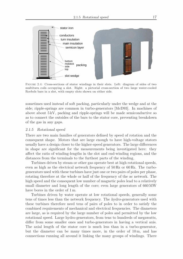
2.1.5 Rotational speed 17
conductorsturn insulation
main insulationsemicon layer
stator iron
bottommidsticksidetop
packing
slot wedge
Figure 2.4: Cross-sections of stator windings in their slots. Left: diagram of sides of twomultiturn coils occupying a slot. Right: a pictorial cross-section of two large water-cooledRoebels bars in a slot, with empty slots shown on either side.
sometimes used instead of soft packing, particularly under the wedge and at theside; ripple-springs are common in turbo-generators [McD93]. In machines ofabove about 5 kV, packing and ripple-springs will be made semiconductive soas to connect the outsides of the bars to the stator core, preventing breakdownof the gas in any gaps.
2.1.5 Rotational speed
There are two main families of generators defined by speed of rotation and theconsequent shape. Motors that are large enough to have high-voltage statorsusually have a design closer to the higher-speed generators. The large differencesin shape are significant for the measurements being investigated here: theyaffect the ratio of winding-lengths in the slot and end-winding regions, and thedistances from the terminals to the furthest parts of the winding.
Turbines driven by steam or other gas operate best at high rotational speeds,even as high as the electrical network frequency of 50Hz or 60Hz. The turbo-generators used with these turbines have just one or two pairs of poles per phase,rotating therefore at the whole or half of the frequency of the ac network. Thehigh speed and the consequent low number of magnetic poles lead to a relativelysmall diameter and long length of the core; even large generators of 660MWhave bores in the order of 1m.
Turbines driven by water operate at low rotational speeds, generally sometens of times less than the network frequency. The hydro-generators used withthese turbines therefore need tens of pairs of poles to in order to satisfy thecombined requirements of mechanical and electrical frequencies. The diametersare large, as is required by the large number of poles and permitted by the lowrotational speed. Large hydro-generators, from tens to hundreds of megawatts,differ from some smaller ones and turbo-generators in having a vertical axis.The axial length of the stator core is much less than in a turbo-generator,but the diameter can be many times more, in the order of 10m, and hasconnections running all around it linking the many groups of windings. There
18 Chapter 2: Stator insulation
is therefore generally a greater ratio of end-winding length to slot length in ahydro-generator than in a turbo-generator.
In the end-winding there is blocking by wooden blocks that maintain separa-tions, and lashing by fibrous bands that bind the windings together, even whenhigh currents exert forces between the conductors; these are seen in figure 2.2.There may be bracing rings to give a strong mechanical support all the wayaround the circumference of the end-winding.
2.1.6 Cooling
Heat is generated by losses in the copper conductors, the iron core and theinsulation itself. To permit high loadings with modest physical size and cost ofthe machine, the temperature rise caused by this heat must be kept low. Thereare several methods of cooling used in different sizes of machine, and all havean influence on aging and diagnostic measurements.
Removal of heat from the windings only after it has passed out through theinsulation is called indirect cooling ; this is normal in small machines, and is usedin some as large as a few hundred megawatts. Removal of heat by a fluid passingwithin the windings is direct cooling. The fluid may be water or hydrogen. Insome cases a few of the conductor strands are hollow to carry the fluid; in othersstainless-steel pipes may be included. The connections in the end-windings aremade with insulating pipes. Hydro-generators use only water for direct cooling,and only on large machines of 500MW and more [Sto04, p.7]. Turbo-generatorsuse water or hydrogen, in sizes from some 200MW and up; in old machinesdirect-cooling may be used in even lower ratings. Direct water cooling resultsin a 100 C limit to the conductor temperature, reducing the thermal stress onthe insulation as long as cooling channels are not blocked; it also gives the riskof leaks that slowly moisten the insulation, although high pressure is used inthe surrounding gas to try to prevent water from escaping.
The gas that circulates within the machine, passing through the coolingducts in the core, over the iron and the outside of the coils or bars, is eitherair or hydrogen. The air-cooled machines are usually at atmospheric pressure.They have the variation of being either open-ventilated using air from outside,possibly through a filter, or recirculated-air with the air sealed in and passing itsheat to external air or water in a heat-exchanger. The hydrogen-cooled machinesare usually at a high pressure such as 3 atmospheres (300 kPa). Hydrogencooling is used in recent machines only above a few hundred megawatts, buthas been used down to 50MW [Sto04, p.6]. An open-ventilated machine hasits components exposed to the external humidity and to fresh oxygen that canreact with hot insulation. On the other hand, recirculated air forces harmfulproducts of discharges, such as ozone, to remain until they have reacted withinthe machine. The absence of oxygen in hydrogen-cooled machines preventsmuch of the oxidative aging that is the major cause of the organic part of theinsulation becoming weak and brittle. The high pressure usual with hydrogencooling increases the breakdown strength of the gas, reducing the tendency todischarges; even when discharges do occur, they cannot produce ozone withoutoxygen, so the wear on the insulation is reduced.

2.2 Failures in stator insulation 19
2.2 Failures in stator insulation
A failure in stator insulation is a low-impedance path between conductors thatare supposed to be insulated from each other, such as those of different turns,bars, or phases, or from phase to core. This section indicates the potentialusefulness of diagnostic measurements [s.4.1] on stator insulation, and lists somecommon ways in which failure occurs. More details are given in later chaptersabout the gradual processes of aging [s.3.2] and about partial discharges in statorinsulation [s.7.5].
2.2.1 Failures of rotating machines
Two ways of classifying failures of high-voltage rotating machines are by thecomponent in which the final failure was seen, or by the suspected root cause. Toa designer the root cause may be of more interest, but for diagnostic purposes theimportant matter is whether the development of a failure would be predictablefrom the studied component. The distribution of failures over components andcauses varies between different types of machine, but a rough indication is givenby the following references.
According to [Tav08, ch.2], which considers all types of rotating machinesincluding low voltage ones, about half of the failures occur in stator insulation.The root cause is usually not direct electrical wear, but a weakness introducedby damage from other mechanisms or by problems in design or construction;the final breakdown of the weakened insulation is then electrical.
In hydro-generators, experience within a large operator is that most failuresare electrical [Hud05], or in other words stator or rotor insulation; it is againnoted that the root causes may be non-electrical. In [Sto04, p.131] a largeIEEE† study is cited as finding about 40% of failures of hydro-generators tooccur in stator insulation; it is also mentioned as an opinion that large turbo-generators generally have a higher proportion of rotor faults. A CIGRE‡ studyof hydro-generators examined 69 failure incidents in detail, and is summarisedin [Bru08b] as finding 56% of the cases to involve insulation damage, with rootcauses determined as 31% aging, 25% contamination, 22% internal PD, 10%loosening in slot or end, 7% thermal cycling or overload, 3% defective corona-protection, and 2% overvoltage. Large studies of failed components and causesin turbo-generators have not been found for comparison.
A study by EPRI§, cited found failures in motors to have root causes located41% in bearings, 37% in the stator, 10% in the rotor, and 12% in accessories.In [Gup96] an IEEE study is cited as finding about a third of ‘forced outages’of large motors to be failures of stator insulation.
In summary of the above, it seems that about a third to a half of failures ofhigh-voltage rotating machines occur in the stator insulation. Even if the rootcause is not the electrical stress, detection of the stator insulation’s deteriorationby diagnostic measurements is a useful way to predict and avoid failure, for thosefailure-types that occur over timescales long enough for warning to be given.
†IEEE — Institute of Electrical and Electronics Engineers (N. America).‡CIGRE — International Council on Large Electric Systems.§EPRI — Electric Power Research Institute (N. America).

20 Chapter 2: Stator insulation
2.2.2 Some stator insulation failure-modes
The stresses leading to failures of stator insulation may usefully be dividedinto two groups: aging [s.3.2] has a gradual effect over a long time, and itscauses such as temperature or working voltage are generally well known andcontrolled; transient stresses occur seldom and generally unpredictably, such asvoltage impulses from the network, out-of-phase synchronisations of a machineto the network, or loose metallic parts flung from the rotor.
These differences in stresses are relevant to the predictability of failures.Immediate failures due to extreme transient stresses clearly cannot be predictedby diagnostic measurements on the stator insulation, even if some might beprevented by checks and measurements on other parts of the machine. Ininsulation that has been deteriorated by aging, the final failure is likely tostimulated by a mild transient stress that would not have been a trouble in newinsulation [Sto04, p.131]. A succession of mild transient stresses may also causeprogressive deterioration, or may cause changes that enable aging mechanismsto have a faster effect.
The remainder of this section brings together short decriptions of some rootcauses and final manifestations of stator insulation failure, including approxi-mate timescales of failure. It does not try to be thorough, as the details areonly used here to give a grasp of the extremes of very mild and more worryingproblems; more detail can be found in [Sto04], [Tav08], [E56] and other booksand standards. The diagrams in figures 5.2 [p.50] and 7.3 [p.90] may be helpfulin considering the mentions of leakage paths and partial-discharge sites.
Failures of turn insulation in multiturn coils also mean immediate failures ofthe machine, often including damage to the main insulation [s.2.1.1] so that theymay appear as main-insulation failures. The turn insulation can be stressed inservice when driven from an IFD [s.7.3.1], with repetitive fast-rise-time pulsescausing large voltages and between the first turns of the winding, with thepossibility of PD. Common offline diagnostic measurements do not stress theturn insulation, so they cannot find weaknesses between turns [Gup96]; testsof impulse-voltage withstand [E792] provide some degree of confidence of turn-insulation quality.
Extreme currents during bad synchronisations, or fault conditions on theelectricity network, cause quadratically increased magnetic force between bars;in the end-winding this can cause loosening of the lashing or even crackingof the insulation. Thermoset insulation, being harder than thermoplastic, isoften more vulnerable [McD93] to looseness of windings and short-circuit forces.Long-term vibration in end-windings with poor lashing and blocking can causedamage to the insulation directly [s.3.2.5], or indirectly by causing problemssuch as water leaks and broken conductors. In thermoplastic insulation systems,where generally the tapes are weaker as well as the asphalt being softer, a girth-crack can occur, where the main insulation is ‘necked’ (thinned) by gradualmovements of the tape layers under thermal cycling [Kle04, p.368], commonlyfew centimetres outside the core. This is sometimes called tape-separation,although that term can be used more generally for loose tapes anywhere. In

2.2.2 Some stator insulation failure-modes 21
rare cases cracks may reach the conductor, permitting contaminants to form amildly conductive path.
Mechanical slot discharge, often just called slot discharge, develops fromlooseness of bars in the slot, due for example to shrinking of insulation orloosening of ripple-springs. The bars can then vibrate in the slot, and havelarge areas without good contact with the slot [Jac82]. This leads to mechanicalabrasion, and to significant contact-sparking that transfer current from the slotsemiconductor to the earthed laminations of the core; the problem is particularlystrong with the harder thermosetting insulation [McD93], which more easilymakes contact with just a few points of the core. The discharges occur as thebar vibrates, so the problem is often impossible to see in offline measurements,and strongly load-dependent† in online measurements. The discharges can bevery large compared to any other PD source within the slot-part of a bar. Theremoval of the slot semiconductor then leads to simple PD in the air-gap betweenthe solid insulation and the core; this ‘stage 2 slot discharge’ can increase thewear rate beyond the effect of the mechanical abrasion. By machine standardsthis is a fast mechanism, taking perhaps two years to failure [Sto04, p.149].
Electrical slot-discharge differs in that there is no need of looseness, theroot cause being a poor semiconductor layer of insufficient conductivity or withvoids between it and the insulation [Sto04, p.152]. Displacement currents in theinsulation must flow out into the core, requiring passage along parts of the slotsemiconductor at cooling ducts and on the faces of the bar that are not in directcontact with the core. Insufficient conductivity leads to excessive heating andconsequent wear, with surface discharges across particularly weak regions. Thedischarges are not specially large, but are generally many. The wear is muchslower than for mechanical slot discharge, more like twenty years to failure.
Regions where layers are not in good contact are delaminations, which canoccur due to poor winding of the mica-paper tape [s.3.2.3], poor impregnation, orstresses in service such as thermal cycling [s.3.2.2]. The spaces thus formed arerelatively short in the radial direction along which the electric field is aligned,but longer in the other directions. Delaminations between layers within themain insulation do not tend to develop in modern Roebel bars, but are morecommon in multiturn coils [Hud05]. Delaminations at the conductors can occurin either type of construction, but are much more dangerous for multiturn coilswhere wear of the thin and possibly non-micaceous turn insulation by PD canlead to failure more quickly than could happen if the whole main insulation hadto be worn through [Sto04, p.146]. The risk associated with delaminations isgiven by [C3427, s.E.1.2] as ‘high’, placing it above all considered sources otherthan slot discharge.
The overlap where the end-winding stress-grading connects to the slot semi-conductor can develop poor contact, particularly when the stress-grading ispainted rather than taped [Sto04, p.155]. There was PD at this point in abouthalf of the hydro-generators studied in [Hud05]. The discharge is across thesurface between the two coatings, and does not cause rapid wear of the actual
†Load-dependent: dependent on the current in the conductors.
22 Chapter 2: Stator insulation
insulation; failure is not very likely even in twenty years. Discharges may alsoappear at the open end of a grading that is too short for its purpose.
Further out in the end-windings, surface contamination with water or dustcan lead to electrical tracking, where the nonuniform conductivity leads todischarges in particular regions, which then become carbonised and more con-ducting, moving the stress out to other regions. A surface resistivity below sometens of megohms allows this to occur [Sto04, p.161]. Tracking may be acrossbar surfaces, or along the surfaces of blocking and lashing between bars. Thetrack of relatively high conductivity grows across the surface, and dischargescan work slowly into the insulation. Failure times can be ten years or more.
Also in the end-windings, insufficient clearances can lead to PD in the air-gaps between the long sides† of bars from different slots, or between the shortsides of bars that share the same slot, or from bars to the earthed metal pressurefingers that sometimes are located between slots [Hud05]. This is much morecommon in air-cooled than in hydrogen-cooled machines, and can be increasedby poorly cured epoxy with abnormally high permittivity. Times to failure bypenetration of the main insulation are five years or more [Sto04, p.168].
†long/short side: consider the cross-sections in figure 2.3 [p.11].

Chapter 3
Aging of Insulation,
Natural and Accelerated
The irreversible changes that gradually occur in an insulation system due tostresses from operation and the surroundings are known as aging. Aging gen-erally makes the insulation less able to withstand the stresses to which itis exposed. This chapter starts by describing common stresses and aging-mechanisms, particularly in stator insulation; it then describes how studies ofinsulation systems attempt to accelerate aging-rates to permit evaluation ofmaterials and test-methods within acceptably short times.
3.1 Insulation aging: mechanisms and synergies
A popular way of dividing the stresses involved in aging of insulation is theacronym TEAM, for thermal, electrical, ‘ambient’ and mechanical stress. Theambient category is the least self-explanatory: it includes for example the effectsof chemicals and radiation.
One type of stress may cause another directly, such as when electrical stressescause PD which generates heat, ionising radiation and reactive chemicals, orwhen differential thermal expansion causes mechanical forces. The aging effectsof one type of stress may change the effects of another, such as when thermalaging reduces mechanical strength or when thermal or mechanical aging pro-duces gaps in which PD can occur. Strong nonlinearity in the effect of eachstress is also to be expected.
These synergies makes investigation particularly difficult: however carefullyone might have gathered results for the effect of, for example, high temperatureor electric field acting alone on an insulation system, the effect of both togetheris only a moderately educated guess.
3.2 Aging of stator insulation
Stator insulation is a complicated construction, both in the radial direction fromconductor to stator core, and in the axial direction from the slot-part through tothe end-winding. There are several interfaces, between metals, semiconductingtape, insulation material and stress-grading, as well as within the compositemica-based insulation material itself; the interfaces are critical points in manyaging mechanisms [Kau02]. The following are the main effects of the TEAMstresses in stator insulation.
3.2.1 Thermal aging
The thermal decomposition of organic insulation materials is a well-establishedfeature of service aging of stator insulation. In air-cooled machines there can be
23
24 Chapter 3: Aging of insulation, natural and accelerated
oxidation and scission of polymer chains [Sto04, p.138], and cross-linking [Tav08,ch.2]. Asphaltic insulation becomes harder, which to some extent may be anadvantage in preventing weak puffy regions of mica caused by migration of softasphalt. Epoxy, however, is only worsened by these reactions, becoming weakerand more brittle. In machines with a hydrogen atmosphere, the generally lowerinsulation-temperatures and the lack of oxygen make thermal aging relativelyunimportant.
A severe case of poorly bonded epoxy-mica insulation after thermal aging isshown in [Bru08b], with many small cavities where PD could occur. The brittleinsulation is more easily delaminated by mechanical stresses, and the cavitiesallow the electrical stresses to cause PD, which in turn produces heat, radiationand reactive chemicals.
The rate of thermal decomposition of organic insulation, even at several tensof celsius above the rated temperature, is often considered as an Arrhenius ratereaction, where an activation energy is needed by the reactants. This resultsin an exponential temperature-dependence: a doubling of reaction rate for anincrease of 10 C is widely assumed for stator insulation [Sto04, p.45]. Thetemperature has to be quite high for this reaction to happen to any considerableextent: thermal stress of epoxy in aging tests is relevant above about 140 C[Bru08a].
3.2.2 Thermal cycling
This form of stress, although originating in changes of temperature, results in amechanical stress on the insulation. Copper has a greater coefficient of thermalexpansion than the modern types of insulation [Sto04, p.45]; the coefficientscan vary as much as ten times between the copper, insulation and core [Kau02].Changes in temperature therefore cause different degrees of expansion in thesetightly bonded materials. The difference in expansion is increased when load-changes happen so suddenly that the temperature in the copper, where mostof the heat is generated, changes significantly without the temperature in theinsulation and core having had time to change.
The differential expansion causes shear stresses at all the interfaces that liebetween the copper conductors and the core: conductor to insulation, tape-layers in the insulation, and bar to core. The mechanically stressed interfacesare susceptible to delaminations [s.2.2.2]. The stresses are greater for longerslot-lengths, such as those of large turbo-generators, and they are enhancedwhen the bars have no external freedom to elongate: thermoplastic insulationtends to expand radially into cooling ducts, locking the outer parts of the barsin place; global VPI on thermsetting insulation also results in bars being lockedinto the slot.
3.2.3 Electrical aging
The main electrical degradation process in micaceous stator insulation is tree-ing [Vog03a], and final breakdown is usually through a tree-channel [Bru08b].Electrical treeing usually starts from an edge of the conductor-bundle [Bru08a][Kim92], where there is high electrical stress and sharp bending of the tapedlayers of insulation [Vog03b]. Even on coils newly manufactured by automatic

3.2.3 Electrical aging 25
taping, there can be considerable imperfections in the layers [Vog06], and ef-fects of other aging stresses can create further such weaknesses. Dominantmechanisms enabling trees to form are thermal degradation of the polymer,mechanical stress from vibration and transient currents, and mechanical stressesfrom thermal expansion [Bru08b].
In pure polymeric insulation, such as plain epoxy or polyethylene, failuresthrough PD in cavities are almost always by treeing [Lau92]. Cavity PD affectsthe polymer surface by heating, chemical effects such as ozone and nitric acid,and ionising radiation [Kre64], and strong local fields from charges in the surfacecan break down the insulation over distances of a micrometre or so, eventuallystarting a tree into the solid from the cavity’s surface. A tree can be initiatedeven without an initial cavity, if local field-concentrations, perhaps caused bymetallic particles, give stresses of some 100 kV/mm, resulting in electrochemicalchanges that can form a small cavity [Bau91]. The subsequent speed of tree-growth is much greater than the speed of initiation, so the total thickness ofinsulation is less important than the stress [Kre64]. Under the very high stressessometimes used in laboratory treeing, the initiation may instead be very quick,for example one power-frequency cycle [Vog05].
Stator insulation is special among high-voltage apparatus, in that it consistsmainly of mica and is therefore highly resilient to internal PD. Mica can degradeunder the combined action of organic acid and ionisation [Jia06], but it gives afar higher strength against treeing than the other components of stator insula-tion. The effect of a thin mica barrier on treeing in epoxy is shown in [Vog05,fig.8], where the tree is forced to detour a long way around the surface of themica. It has been observed that treeing in stator main-insulation is never direct,but goes a long way around the mica layers, getting through particularly easilyat points of imperfections such as delaminations, cracks and cavities [Bru08b].
The power-law relation of electrical aging to applied voltage is often used,although the exponent itself may vary: “The relationship between failure timeand voltage follows the inverse power law” [E434]. An exponent of 7 to 9 isgiven in [Kre64] for general PD and treeing. In [Sto04, p.46] an exponent of 9to 12 is given for the effects PD in stator insulation, and the effect of electricalaging is considered to be zero below some threshold voltage.
The mechanism of breakdown by electric stress changes with the level ofstress. For stator insulation [E434] the moderate stresses and long lifetimesfound in service can lead to breakdown through erosion from PD and ‘elec-trochemical attack’, as discussed in the above description of treeing; at thehigher stresses and consequently shorter times that might be found in extremelaboratory tests, a thermal mechanism due to losses may be dominant; higherstill, discharges with high charge-concentration break down insulation aroundtheir tip, in ‘streamer breakdown failure’.
An increased frequency of the applied voltage has sometimes been used,such as hundreds of hertz up to some kilohertz, to study electrical aging at anincreased rate [Sto04, p.62], on the assumption that a certain amount of PD ortreeing occurs in each cycle. A review [Joh79] suggests there often is a strongproportionality of these types of aging to frequency, but not reliably enough to

26 Chapter 3: Aging of insulation, natural and accelerated
warrant standardisation.
3.2.4 Ambient
One class of ambient stresses comes from the atmosphere in the machine, whichmay contain water vapour, oxygen and possibly ozone and other reactive gasesfrom PD activity. The presence of dust or salt in the air around an open-ventilated machine may cause blocking of cooling ducts and contamination ofthe winding surfaces [E56]. Oil from mechanical parts in the machine or fromoutside can slowly degrade the organic insulation. Water penetrates quickly intoasphaltic insulation, causing swelling and weakness, more slowly in polyester,causing depolymerisation, and over timescales of months or years even intoepoxy insulation [Sto04, p.166].
3.2.5 Mechanical stress
The currents flowing in the windings cause oscillating forces between bars, attwice the power frequency. Looseness of bars in slots or of the lashings in theend-windings permits relative movement, which can lead to cracking, delami-nation and abrasion [Tav08, ch.2]. Particularly strong forces occur during faultconditions in the external network: these may cause immediate damage. Therelation of lifetime to the stress of mechanical aging by vibration is sometimestreated as inverse power law [Wei05].
3.3 Accelerated aging
When a new material or new construction of insulation system is proposed, orwhen an existing insulation system is to be subjected to a previously little-testedcombination of stresses, tests are needed that will provide some idea of lifetime,at least by qualitative comparison with well-known insulation and stresses. Theinsulation of stator-windings has a typical design-lifetime of more than twentyyears, so any ‘natural’ aging should result in few failures even after decades. Aquicker type of test is clearly necessary, to permit development and applicationof new insulation systems within a reasonable time and to avoid the high costof keeping tests running for long periods.
One method is to study relatively easily-measured material properties suchas breakdown voltage or abrasion-resistance, and to infer from these the suit-ability of a material for its intended use [Sto04, p.68]. In view of the complexityof typical insulation constructions and failure mechanisms, there is only weakjustification for the assumed relations between the properties of constituentmaterials and the performance of the whole system under multiple stresses.Other types of tests are obviously desirable for better confirmation. An accel-erated aging test is performed on objects that are more or less similar to thereal insulation system, for example real stator bars in model slots, but makesat least one stress be higher than in service, to shorten the aging time. Thediscussion of aging in stator insulation [s.3.1] gives indications of how sharplythe levels of stresses may affect the aging rate.
Accelerated aging may also be useful for the evaluation of new diagnosticmethods, and for establishing criteria for interpreting the results. In thesesituations the use of real insulation systems under natural service conditions has

3.3 Accelerated aging 27
several problems. One is the slowness of the changes due to aging, although thisis not so critical as in design, since measurements can be made on a wide rangeof ages of existing machines. Another is the availability of sufficient numbers ofmachines on which down-time can be accepted for making measurements. An-other greater problem is that the relation between measurements and subsequentfailures of the insulation is not easily obtained: in particular, it is unlikely thatapparently bad insulation will be left in service just to check whether the verdictof badness was correct. Even if accelerated aging cannot be considered to bevery realistic, its advantage of permitting multiple objects to have measurementsmade regularly, up to failure, and within practicable timescales, may make itworth using as one way of testing new diagnostic methods and criteria.
The simplistic description of accelerated aging is that a fairly similar effectto the natural aging is made to occur in a shorter time. Bearing in mind thesynergies involved between different stresses in service, and the likely variationin the stresses caused by operation of similar machines in different environmentsand applications, little confidence can really be had about similarity of the insu-lation’s state after ‘service’ or accelerated aging. The realism of the accelerationdepends at least on the acceleration-factor being not so high as to modify thedominant aging-mechanism; for example, this would happen if an acceleratedvoltage-stress causes abnormally high temperature, or causes discharges wherethere never would be any in normal operation.
Several forms of accelerated testing are widespread enough to be the subjectof standards, such as functional evaluation of mica-based main-insulation forhigh-voltage stators [E434] by thermal, electrical, cyclic and mixed stresses,as well as even more specific standards for thermal-cycle testing [E1310] andvoltage-endurance [E1043].
The standards avoid claims of direct similarity to effects of service, settingout only to provide a method by which different groups of test objects, such asan established and an experimental insulation system, can be compared. It isimplicit that the accelerated methods of the standards will give results that arecorrelated to those that would be seen in service.
There are several ways of assessing which group performed better: a testimposing a fixed stress for a fixed time may be made at intervals betweenperiods of accelerated aging, until the specimen fails; alternatively, a guaranteeddestructive test such as a breakdown-voltage measurement may be performedafter a single fixed time of aging; nondestructive methods compare results ofmeasurements such as PD and DS, appearance, mechanical properties, chemicalor physical composition, or emission of particular chemicals.
The ‘equivalence’ of aging mechanisms in test and service should be verified[E943], particularly for higher degrees of acceleration. Examples of verificationsare a qualitatively similar pattern of PD pulses, or the same location and typeof failure in destructive tests, at different levels of stress. Other factors thatmight influence the aging should be kept close to the values expected in service:examples are any surrounding gas or other medium, or whether heating occursfrom inside or outside a stator-bar.
The standardised methods of accelerated testing generally use only one
28 Chapter 3: Aging of insulation, natural and accelerated
accelerated stress, other stresses being either absent or at the levels foundin normal service, although one group of test-objects may have multiple highstresses to give an idea of the combined effect [E434].
Complications arise when simultaneous applications are made of morethan one factor, even if only one of the factors is intensified.[E943]
It is not even obvious that all types of stress will have a monotonic effect whenin combination: for example, the increased flexibility of epoxy-mica insulationat higher temperature can give several times higher endurance of mechanicalstresses at 90 C rather than at room temperature [Wei05], with the combinationof mechanical and thermal aging effects minimised at about 135 C for modernepoxy-mica [Bru08a]. The means of acceleration may be more imaginative thanjust a direct increase of a stimulus: for example, extra-long bars can be madeto increase the degree of mechanical stress during thermal cycling [E434].
The amount of variance between results on supposedly similar specimens,whether aged by service or in an accelerated way, clearly makes it necessary touse several specimens in each group. The prescription of [E434] is to use at leastfive, and preferably ten, and to use at least three levels of stress.
The Weibull distribution is commonly used in reliability studies. It is well-suited to fitting the ‘weakest-link’ properties typical of lifetime data. Differentmechanisms of failure can sometimes be distinguished by the Weibull parametersneeded to fit the results [Tav08, ch.3]. Some examples of Weibull plots for variedstress and varied insulation can be seen in [Bru08b]. When the lifetime as afunction of stress requires different Weibull parameters over different ranges ofstress, this suggests changes in the dominant mechanism of failure, which wouldmake assumed acceleration factors invalid.

Chapter 4
Diagnostics and Prognostics
High-voltage insulation systems in power apparatus are given many tests andmeasurements during design and manufacture, before delivery, on installation,and throughout their lifetime. The results are used to verify suitability of a newdesign, verify quality of a batch, optimise planning of operation and maintenanceof the apparatus, or locate a suspected defect.
The manufacturer-oriented measurements have been sufficiently covered insection 3.3. This chapter considers measurements made by end-users duringthe service life of an insulation system; this category includes the types ofmeasurement studied in this work. The focus is not technical details of themeasurements but a discussion of the aims of collecting and analysing data,and some important categories of measurement. Stator insulation is used forexamples throughout the chapter, and current practice for measurements andinterpretation of stator insulation is summarised at the end.
Some words are used in this chapter in senses more specific than theireveryday use. A test gives a simple result of pass or fail; in the high-voltagecontext this probably involves subjecting insulation to a level of electric stressgiving a much increased risk of failure. An inspection gives a result through thehuman senses, such as checking colours, sounds, smells or looseness; it involvesno electric stresses. A measurement gives a more complicated result than a test,needing interpretation, and uses stresses expected not to make the failure-riskmuch greater than in normal operation; in this chapter the definition is takento include inspections. A method is used as a rather vague term for a particularmeasurement and its interpretation, or a group of measurements.
4.1 Diagnostic and prognostic aims
The terms diagnostic measurement and condition assessment are widely usedto describe measurements made on insulation systems: both terms suggest thedetermination of a current physical state rather than the assessment of futurebehaviour. If an apparatus has already failed and cannot be used, a purelydiagnostic measurement and interpretation may help to identify the problem’stype or location, as a step to correcting it. Otherwise, the diagnostic step isnot directly useful in itself: some sort of prognostic step is needed from whichdecisions can be made about operation and maintenance. The term prognosticmeasurement would seem more appropriate to many of the measurements madeon stator insulation by end-users, but ‘diagnostic’ is firmly rooted in use. Thedistinction will be preserved only in this chapter: in the rest of this work, just thediagnostic step from measurements to an estimate of current state is attempted.
The impossibility of precise prediction of failures, which often depend onlocalised ‘weakest link’ breakdowns in response to unexpected disturbances
29

30 Chapter 4: Diagnostics and Prognostics
such as transients, may make a suggestion of prognosis or lifetime estimationseem foolish. But regardless of the term used to describe the conversion ofmeasurement data to decisions about operation and maintenance, there surelyis a prognostic element involved, however implicit it is in the procedure.
“Prediction is very difficult, especially about the future.”Niels Bohr
The prognostic aims are quite different from the pure sense of a diagnosticprocess as the determination of present state. A diagnostic result makes a moreor less specific claim about some feature of state: for example, ‘there is a mildlyconducting path between the conductors and earth’, or ‘the epoxy is stronglydepolymerised, with poor binding and many small cavities’, or ‘there is at leastone delamination next to the conductor stack’. A prognostic result makes amore or less explicit claim about future behaviour: for example, ‘this level andtype PD of is usually followed by failure within a year’, or ‘this insulation seemsgood as new’, or ‘company policy for a winding giving results in this range isthat it should be returned to service and have a further measurement after twoyears’.
4.2 Obtaining and interpreting data
An attempt is given in figure 4.1 at a description of the process of collectingrelevant data about an apparatus and making decisions from it; this is supposedto be general enough to represent data and rules ranging anywhere from vaguenotions in one person’s head through to carefully recorded details and rules usedin a large organisation or a computer program.
prognose
diagnose
statestimulate
prognose
decideaction
apparatusdata
rules for all judgements
(possibly updated by experienceon this and other apparatus)
stateestimate
history
Apparatus
measure
Exchange/Comparison of results
−− earlier measurements (trending)−− other phases in the same component−− other components of similar designs−− other mildly similar components
prognosis
maintenance
Figure 4.1: The generalised diagnostic/prognostic process. Triangular blocks are actions,such as judgements based on input data and rules. Circular blocks represent measured orinferred knowledge. The heavy lines in the top right are the main prognostic process; thelighter lines provide data for assessment and revision of the rules.
An apparatus whose exact physical composition, or state, was guaranteednever to change would have the same chance of failing at all times, given the
4.2 Obtaining and interpreting data 31
same stresses: no useful purpose would be served by making routine mea-surements on it. The state of a real insulation system does vary, and affectsthe chance of failure: the variation includes reversible short-term effects, someexamples of which are given in chapter 16, and irreversible effects of the long-term aging-processes discussed in chapter 3.
The diagnostic or prognostic result is based on apparatus data and onrules stating how to convert the data to results. The apparatus data makesthe necessary link between the state and the diagnostic or prognostic process.Part of the apparatus data may be ‘history’, based on operational conditionsexpected to have had some influence on the current state. Examples includeloading, ambient temperatures and humidities, winding-temperatures, PD dur-ing service, cleaning, and ‘traumas’ such as transient voltages and out-of-phaseswitching. The other part of the apparatus data may be ‘measurement’ of quan-tities that are determined by the current state. Examples include polarisationand conduction currents, partial discharge, and results from visual inspections.Measured data may be able to be obtained without added stimulus, as for onlinePD measurement or offline inspection of insulation-surfaces, or it may requirecontrol of the stimulus as for an offline PD measurement at varied voltage.There is not a rigid division of phenomena into those that purely affect andthose that are purely affected by the state: the above example of PD can be inboth categories.
Having gathered apparatus data, rules are used to make diagnostic or prog-nostic inferences. The diagnosis estimates an aspect of the state, such as thepresence of some minimum size of PD cavity, a conductive path between surfacesof end-windings, or a degree of degradation of a material. In view of themany types of problems that can occur in a complex apparatus, a sensiblediagnosis may well return a range of possible states that would fit with theapparatus data. One automated ‘expert’ system [Sto04, p.231], which canbe seen as explicitly going through many of the steps that a human expertwould take, presents not just the one or several proposed diagnoses but also adescription of why these were chosen, a list of other possibilities that came close,and suggestions for what further measurements would most effectively resolvethe diagnostic question. Although the above examples of diagnoses sound likemodel-based inferences that would be based on considering physical modelsof the apparatus and the ‘inverse problem’ back from measurements made onits state, the alternative data-based approach could be used instead, based insome way on correlations observed from previous apparatus data and subsequentrevelations of the state from further inspection. For the diagnostic step the data-based approach seems an unlikely choice; some of the ‘measurement’ data ofinspections would presumably be the ultimate source of testing the correctnessof inferences made on the remaining data.
Having reached the diagnostic estimate of state, the work is finished if thesole aim was to decide the most likely type of fault in an apparatus that alreadyhas been decided to need repair. In most cases it is actually the prognosticresults that are desired. The prognosis is shown as following two possible routes.The lower route is direct from apparatus data to the prognostic result; this
32 Chapter 4: Diagnostics and Prognostics
implies a data-based approach, probably working from statistics of historicaldata. The upper route may also be a data-based prognosis, but with its inputfrom the estimated state of the diagnostic step rather than from the raw data;otherwise it may be a model-based prognosis, using physics-based considerationsto predict future changes in the apparatus.
4.3 Maintenance decisions
From the prognostic result, decisions must be made about what action to take:what maintenance, if any, should be performed; should there be any change inthe operation of the apparatus; when should the next assessment be made? Theoptimal decision depends both on the apparatus and on what application it isused in, as well as on the reliability of the prognostic process.
The relation between apparatus data and the correct prognosis is determinedby the construction of the apparatus and the loading that will be put on it by itsapplication. The relation between a correct prognosis and the correct decisionis determined by the costs of all the alternative actions and the probabilitiesassigned to them based on the prognosis. Costs may be due to the repair of afailed apparatus, unplanned downtime or damage to the apparatus’ applicationdue to a failure, or costs of planned downtime and work if maintenance isperformed. The prognosis may be wrong, giving a clean bill of health toan apparatus that has a severe weakness, or recommending downtime andmaintenance of an apparatus that could have survived for years. This is relevantwhether the prognostic result is a probability distribution or a run/stop value.The decision-making should take into account the probabilities of these errorsand their costs for the particular apparatus and application.
The many types and applications of motors and generators result in widevariations in the balance of costs of faults occurring versus costs of measure-ments and maintenance. Extremes are small, cheap, easily-replaced machinesin noncritical applications, and machines that could take weeks to repair afterfailure and would cost vast sums per hour of lost operation, such as a largegenerator in a nuclear power-station. The amount of attention given to makingand interpreting measurements and to performing maintenance is thereforealso very varied. In the relatively high-power machines for which this workis relevant, the machine itself is expensive and not easily replaced, and itsunavailability is likely to have a high cost. It is unlikely that pure ‘correctivemaintenance’, of waiting for failures to happen, will be used; some degreeof prognosis will be made to allow ‘predictive maintenance’ even in the less-critical cases. Some suggestions for policies of measurements and maintenancein different applications of machines are given in [Sto04, p.351].
4.4 Establishing and updating rules
Rules are used at each stage: they can be seen as determining even what datashould be gathered, as well as how the subsequent stages of inference shouldbe made on the data. Rules for a data-based method may be anything from arule-of-thumb of long-forgotten origin and without any verification, through aregression analysis of historical measurement results and failure data, up to a

4.5 Measurements offline and online 33
Bayesian model [Lin08] with continual fine-tuning of rules in the light of newinformation [s.A.2.5]. Rules for a model-based method may be based on any-thing from microscopic phenomena to equations based on sample-measurementsrepresenting some component of the apparatus.
Regardless of how they are chosen, the rules will be severely imperfect. Thediagnostic, prognostic and decision problems are difficult ones to study: theactual service conditions vary, failures cannot be reliably predicted from modelsof deterioration processes, accelerated tests are only an approximation of effectsin service, and good life-data for real aging up to a natural failure is hardto obtain. Some large databases covering routine diagnostic measurements onthousands of generators and motors have been built up by large owners andconsultancies. Even in these there will be long delays, of the order of decades,between starting to use a model of apparatus and getting a useful amount ofdata about its failures. It is unlikely that checks will be made of whether aprediction of imminent failure would actually have turned out to be true, so it ishard to get strong supporting evidence for later predictions; less realistic checkssuch as quick overvoltage-testing and dissection after removal from operationare probably the best methods available in practice. Part of this problem of‘censored’ data where failures have not yet occurred or apparatus was retiredbefore failure occurred, is discussed in [Lin08].
A good system for diagnostic or prognostic results will not just choose somerules and leave them, but will take advantage of experiences gained during itsuse, to consider adjusting its rules. The dashed arrows into the ‘rules’ box in thediagram carry information about data, diagnoses, prognoses and decisions. Thisinformation can be linked to external information that confirms or contradictsthe goodness of the inferences, for example an inspection performed after adiagnosis or a failure after a prognosis. The arrow to ‘other apparatus’ shouldbe an important part of the setting of rules: it is likely that much of the initialrule-set for an apparatus will be based on experience with other more or lesssimilar apparatuses, and the changes to the rules should likewise be based onall the relevant data that is available.
4.5 Measurements offline and online
An offline measurement requires the apparatus to be out of service. This is truefor the methods studied in this work: they require the applied voltage to havewidely varied amplitude and frequency, and the winding to be isolated fromearth and preferably split at the neutral point to allow separate treatment ofthe phases. An online measurement is made when the apparatus is in operation,giving an immediate advantage of avoiding downtime. An extreme case of onlinemeasurement is online monitoring, where a measurement-system is permanentlyconnected during operation of the apparatus.
Inspections involving some disassembly, such as visual inspection of slot-wedges and end-winding insulation surfaces, will require the apparatus to beoffline. Electrically-based offline measurements may need a separate power-source, which for large apparatus at high voltage and power frequency can beexpensive and large. An advantage gained is the ability to control the voltage to

34 Chapter 4: Diagnostics and Prognostics
obtain extra information: the PD inception and extinction voltages, PDIV andPDEV, are commonly measured in offline PD measurements, requiring variationof a sinusoidal excitation. By selecting different combinations of high-voltageand earth potentials in a multi-electrode system, specific parts can be stressed:offline measurements on stator windings usually excite one winding at a timethen all together, helping to distinguish defects between phase and earth fromdefects between phases. Offline measurements also tend to have the advantageof lower noise, permitting better measurements of PD and measurement of thesmall current in the insulation.
Online methods allow measurement of phenomena that actually occur duringoperational levels of parameters such as gas-pressure, temperature, forces onconductors due to load-currents, external vibration and voltage-stress. Theyalso allow variation of certain parameters, such as conductor temperature, orvibration from load-current, that cannot easily be controlled when not in op-eration. Studying a parameter such as PD over a range of load-currents ortemperatures may help to detect defects or distinguish between possible loca-tions of a defect: for example, mechanically induced slot-PD is heavily increasedby high current-loading.
The realism of the stresses during online measurements does not make onlinemethods unconditionally superior. The important aim is to make a good diag-nostic or prognostic inference. If a particular measurable phenomenon, such asvibration-dependent slot-PD, occurs under online conditions but may be missedin offline measurements, and if this phenomenon is strongly related to dangerousdeterioration as either a symptom or a cause, then the online measurement hasan advantage. But the same is partly true the other way round: a phenomenonthat can be detected by offline but not by online methods, such as a crackthat is only noticed by measuring small currents through the insulation at highvoltage and low frequency, will put the offline method at an advantage, as longas this phenomenon is a symptom of dangerous deterioration; the differencefrom the previous example is thus that a phenomenon which occurs only inoffline measurements and is a cause but not a symptom of deterioration, is not
a useful indicator of a problem but merely a good reason to stop the offlinemeasurement.
The above comparisons suggest that the offline and online methods arecomplementary rather than directly competing; it is common to use both. Forexample, when online stator PD measurements suggest the start of a problem,offline measurements are recommended [E1434, p.30] to gather further informa-tion before deciding what further action to take.
Online monitoring typically has automation of data collection, with differentlevels of alarms to alert operators to probable urgent problems and alert onlymaintenance staff to problems predicted to be too distant to worry about im-mediately. The frequently-logged data permits extremely fine trending: insteadof having to compare results with a few previous measurements at one-year orperhaps five-year intervals and at probably rather different temperatures andhumidities, the entire past behaviour of the apparatus is available for assessment.
4.6 Cross-comparison, trending, and relative measures 35
4.6 Cross-comparison, trending, and relative measures
A recurring theme in standards and recommendations about interpreting mea-surement data, particularly for prognostic purposes in machines, is that trends,and comparisons with similar objects are generally better guides than tryingto set limits for a whole class of apparatus. In some cases, such as PD mea-surements on polymeric high-voltage cables, any detectable PD is worrying,so there is some sense in responding to a single measurement without makingcomparisons; even here a rapidly growing level seen in online monitoring wouldbe more worrying than a steady level. In stator insulation, PD at tens of timesthe detection-level for a cable would be mild, and is to be expected throughouta long and happy service life: a lot more detail than the existence of a moderatesize of PD is needed for a good prognosis.
In the absence of other knowledge about limits, comparison with the mostsimilar apparatus that has not yet failed is a reasonable way to make a simpledecision of fitness for service. An example of the importance of similarity is thedependence of signal attenuation on winding-construction; similar PD sourcesin machines with different winding-layouts may show very different results inmeasurements. A comparison with an identically constructed apparatus avoidssome such problems, but does not help with some other causes of differencesin results, such as different ambient conditions between the two apparatuses.For stator insulation, the presence of two other phases usually of very similarconstructions and in very similar ambient conditions, permits useful comparativemeasurements.
Even comparing between phases in the same stator, there is the problemthat similar deterioration may appear differently in measurements dependingon its position within the test-object and reference-object. For example, similarPD sources in different parts of a winding may give very different results. Atthe expense of the guarantee of similar ambient conditions, a comparison canbe made between previous measurement occasions on the same object, allowingfor example a source of unusually large PD pulses to be treated as less worryingif it has been constant or slowly increasing over several occasions than if it hasrecently appeared.
A focus on changes and their relative values is a common way to reduce theeffects of slowly-changing disturbances and differences in instrument calibration.External factors such as atmospheric conditions and apparatus temperature caninfluence measurements, making direct comparisons between occasions difficult.Significant differences in calibration may exist between instruments, and in-struments may themselves be temperature-dependent; small differences in largemeasured quantities may be obscured by the calibration difference betweenmeasurement occasions.
Temperature and humidity have a strong influence on measurement of in-sulation resistance (IR) [s.6.4.2]. Use of the ratio (PI) between IR values attwo or more time-points in a single measurement solves much of the problem oftemperature-dependence, as well as dividing out the effect of test-object size.
Calibration differences as well as temperature effects would affect the smallvoltage-dependent changes due to PD, in the large values of capacitance and loss

36 Chapter 4: Diagnostics and Prognostics
in stator insulation. The ‘tip-up’ measurements [s.6.4.1] of capacitance and lossrecord variations with voltage, between results obtained with one instrumentat immediately consecutive times; they can therefore be compared betweendifferent measurement occasions with much less sensitivity to calibration.
Measurement of PD on stators cannot be calibrated into apparent charge atthe PD source, and differences in instruments and test-circuits may make eventhe relative sizes of different PD sources within a measurement vary betweenmeasurement occasions. This is not so simple a problem as an error of scale-factor, but on the other hand the stochastic nature of PD reduces the degree ofprecision that is ever expected in a PD measurement. PD is normally recordedas absolute values; that is, relative only to a calibrator, not for example to themaximum charge. A phase-resolved PD pattern is, however, often interpretedas a pattern, where the general shape is more important than the registeredcharge; in this respect a PD measurement can also be seen as using relativevalues of results to avoid some of the differences caused by instrumentation.
A final consequence of the dependence of so many measured phenomena onexternal factors is the importance of recording the factors most likely to beimportant, along with measurement data. The atmospheric temperature andrelative humidity are significant in all high-voltage measurements on machines;pressure is important too when external PD is involved. Other details such as in-ternal temperatures, the degree of disassembly or the layout of test-connections,may be useful when later using the data; photography can help to capture a lotof this information in a short time.
4.7 Current practice for stator insulation
Elaborate protection systems are used on large machines, for rapid disconnectionafter detection of a fault in the machine or a form of operation that will harmthe machine. They protect the network from a faulted machine and preventfurther damage to the machine. These systems include ‘relays’ that detect over-current and earth-faults, under-frequency and over-frequency, voltage-imbalancebetween phases, and more [Tav08].
In contrast, the ‘diagnostic’ (although ultimately for prognostic purposes)and ‘monitoring’ methods are intended to allow faults to be predicted in enoughtime to reduce unplanned downtime and damage to the machine. The maintypes of data gathered about stator insulation are listed below; more detailabout these and methods for other parts of rotating machines can be foundin [Sto04] and [Tav08]. Using several types of measurement allows a betterassessment of the insulation’s condition.
The removal of a generator’s or motor’s covers and rotor, followed by in-spection of insulation surfaces, end-winding blocking and lashing, insulationfirmness, and tightness of wedges and bars in slots, is held as one of the mostuseful sources of information about the insulation’s state [Sto04, p.229]. Thishas of course the disadvantage of being an offline method and of requiring furthertime for the disassembly.
As a rather detailed investigation of insulation condition, bars can be re-moved from a few points around a winding, replaced with spare bars, and the

4.7 Current practice for stator insulation 37
removed samples can then be subjected to destructive tests such as voltage-endurance and dissection.
Partial discharges are very commonly measured in stator insulation, onlineand offline; this is covered in chapter 8. The currents in the insulation, includingin some cases PD currents, are commonly measured offline by methods knownas insulation resistance and tip-up, covered in section 6.4.
Temperature measurements online are very common and have been used fordecades. The sensors may be placed at points in many of the slots, typicallybetween bars for a good measure of the insulation temperature. Results fromend-winding sensors depend also on the surrounding gas temperature; ther-mography by heat-sensitive cameras can instead be used to check end-windinghot-spots. Temperature may reveal problems with electrical cause, such as aworn semiconductor layer, or other sources of overheating that may affect theinsulation.
Chemical measurements are made online to detect the chemicals and smokeparticles from overheating of organic insulation (generator condition monitor,GCM, or core-monitor); this is relevant to insulation between core-laminationsas well as to stator insulation. Tracer-paints can be put on parts of windings, torelease distinguishable chemicals from different parts of the winding at differenttemperatures. The complicated matters of rates of generation and loss of chem-icals, and gas volume and detection thresholds, limit the sorts of overheatingthan can be detected in this way [Tav08, ch.3]. Ozone from partial dischargesis commonly measured online, as an occasional measurement or a monitoringsystem.
Vibration monitoring may be performed on various parts; in many casesthe vibrations are concerned with rotor and mechanical problems, but excessivevibration of end-windings may have consequences for stator insulation.
A commonly used test, in the sense defined at the start of this chapter, isthe hipot (high-potential) or ‘pressure’ test, where a voltage considerably higherthan the normal service level is applied for a time in the order of one minute.The chosen voltage is not widely standardised but is generally well over twice theservice level [Sto04, p.243]. The result is then a simple pass/fail depending onwhether a breakdown occurred; this makes clear that it is not worth doing sucha test on a machine whose in-service failure has little cost beyond the machine:a hipot failure may happen even on a winding that would have survived longin service. A dc hipot test permits a small supply, but the field-distributionin the insulation may be very different from the field in service. The currentmay be measured too, to get a more detailed result than the simple test. Hipottests with ac may use normal power frequency, or may use low frequencies suchas 0.1Hz to reduce power-supply demands but keep an approximately ac field-distribution [E433]. A summary of relative advantages and disadvantages of acand dc hipot is given in [E95]. Another form of overvoltage test, designed to testthe turn insulation, is the surge test [Sto04, p.265], injecting a high-frequencypulse into the winding; this stressing of the turn insulation is in contrast to theother offline electrical methods.

38 Chapter 4: Diagnostics and Prognostics

Chapter 5
Dielectric Response
Conduction and displacement currents within an insulation system are measuredin several common diagnostic methods. This chapter describes the origins ofthese currents, moving from simple homogeneous and isotropic materials to thecomplicated structures of high-voltage insulation systems. Stator insulation isthen considered, from the dielectric properties of constituent materials and thecomposite insulation system that they form, to the effects of different formsof deterioration upon the measured current. Common ways of measuring thecurrents for material studies and for diagnostic purposes on insulation systemsare described in chapter 6.
There are many books available about dielectric response: a good expositionof models and mechanisms is given in [Jon83] along with data from a wide rangeof solids; an overview of mechanisms and measurement methods is also givenin [Hel00], which has the advantages of easy availability and a focus on pristineepoxy-based stator insulation.
5.1 Basic electrical properties of materials
Every material contains positive and negative charges on which an appliedelectric field exerts forces in opposite directions. Most charges are not free tomove more than fractions of an atomic size within a material under an appliedelectric field. Except in a plasma, charges are mainly bound to opposite chargesto form neutral atoms and molecules, with bonds stronger than macroscopicelectric fields found in normal service of high-voltage equipment.
An electric field applied to non-free charges causes polarisation, a limiteddisplacement between the positive and negative charge-centres. When the ap-plied electric field changes, there is a new steady-state value for the polarisation:the change in polarisation towards this steady state is the dielectric relaxation.Different mechanisms of polarisation give rise to a vast range of relaxation times.Pure dielectric response, DR, is the dynamic behaviour of the polarisation inresponse to an applied field. Measurements referred to as DR often includeother phenomena such as free-space capacitance and conduction, sometimes asdesired extra information and sometimes as an undesired disturbance.
A conductive material contains many charges that are free to move through-out the material, such as conduction electrons in metals, or ions in solutions.These are generally a distinct minority of the total charges in the material,but even a single free charge per several atoms results in strong conductivity.Copper, for example, has a conductivity σ = 6×10⁷ S/m, relating current-density of the moving charges to an applied electric field E; expressing thisas 6 (kA/cm2)/(V/m) makes clear what a large current-density this entails evenfor a tiny electric field.
39

40 Chapter 5: Dielectric Response
The conduction and polarisation processes are generally distinct and largelyindependent [Jon83, p.47]. Polarisation of the bound charges in a good conduc-tor is not usually of interest, as the achievable fields in the material are so weakand the conduction currents are so much stronger than any measurable effectof polarisation. Polarisation is therefore a phenomenon associated with poorconductors — semiconductors and insulators.†
High-voltage insulation uses only good insulators such that the typical ser-vice stresses of easily 3 kV/mm cause conduction currents in the order of nanoampsdown to femtoamps, in spite of the large conductor-surface of a cable or winding.For example, the XLPE (cross-linked polyethylene) widely used in power cableshas a resistivity at room-temperature in the order of 1016 Ωm, corresponding tosome 100 (pA/m2)/(kV/mm).
True conduction through a material is a process in which the charge densitythroughout the material can stay constant but charges keep moving between theelectrodes. A conduction current is thus sustainable for any period and stores noenergy. In insulating solids, electrons are made available for conduction by thepresence of impurities or by thermal energy. The conductivity can increase byorders of magnitude when temperatures change between ambient temperatureand the typical working temperatures just some tens of celsius higher; thisis in contrast to good conductors, whose conductivity decreases, much moregradually, with increased temperature. A strong field in an insulator may affecthow many charges are available for conduction, but at weaker fields the availablecharges are largely independent of the field.
Polarisation within a material changes the electric displacement field. Therate of change of this field with time is the displacement current, so changesof polarisation result in a particular type of displacement current, polarisationcurrent. In a good insulator the small conduction current and the strong electricfield that can be built up permit the polarisation to be the dominant cause ofcurrent even at the moderate frequencies of power frequency and lower thatare considered in this work. Polarisation changes the charge densities in thematerial, and cannot continue for ever; energy is stored by polarisation, andsome of it can be returned.
DR measurements on materials are typically used to assess the compositionand freedom of molecules. This is of interest in several disciplines, among themchemistry, polymer and solid-state physics, semiconductor and insulation engi-neering, and some biological applications. Between these disciplines there aremany different names, equations and types of plot used to describe and presentthe same concepts; even within the ‘insulation community’ there are differencesbetween countries and periods in the choice of terminology. A description ofthe relation between many industrially oriented terms for dielectric propertiesis given in [T150]. The following section includes names and notation for themain features of dielectric response that are discussed in this work.
†The distinction between a dielectric and an insulator is a matter of application ortaste. Both words are used for materials that can keep conductors electrically separated,withstanding high fields with minimal conduction; if high polarisability is a desired feature,as in a capacitor, then the material will probably be referred to as a dielectric.

5.2 Mechanisms and descriptions of dielectric response 41
5.2 Mechanisms and descriptions of dielectric response
Measurements of dielectric response usually consider just a narrow band of thewhole range of times or frequencies over which polarisation mechanisms operate.The mechanisms with significant dynamics in this band are the interestingdielectric response, and other mechanisms are treated as instantaneous if muchfaster or as nonexistent if much slower.
Even across a vacuum an electric displacement D† occurs in response to anelectric field E, related by the free-space permittivity ε0 as D = ε0E. Thesignificance of D to measurements is its relation to charge-density = ∇·D; itssurface integral determines the charge on an electrode whose potential is heldconstant by an external circuit, and the time rate of change in this charge is themeasured current in the circuit. Polarisation in a material increases D by thetotal volume-density of dipole moments, Pt, so that D = ε0E + Pt.
In practical insulation materials exposed to service-levels of electric fieldthe steady-state polarisation is very close to proportional to the electric field,and therefore gives the same effect as an increased ε0. The total electricdisplacement can then be treated as a part due to free-space and a part due to allpolarisation, or at the other extreme as a single effective permittivity ε with noexplicit polarisation term. An intermediate form is relevant to cases where somepolarisation takes long enough that it is not practically instantaneous comparedto the changes in electric field being measured, and therefore cannot be includedin a constant ε: the free-space permittivity together with the components of thepolarisation that are practically instantaneous are the prompt response, treatedas a single value of high-frequency permittivity ε∞, and the remaining, slowerpolarisation P is kept separate. These three ways of distributing the polarisationbetween an explicit and implicit part are
D = ε0E + Pt
= εE
= ε∞ E + P. (5.1)
The fastest polarisation mechanisms are the induced polarisation displace-ments between electrons and nuclei or between ions in a lattice, happeningin times short enough to correspond to optical or infra-red frequencies, andwithout strong temperature-dependence. Slower mechanisms that give dynamicdielectric response at the frequencies met in electric circuits are dipolar, carrier-dominated and interfacial polarisations. Interfacial polarisation is a consequenceof inhomogeneity rather than a microscopic feature of a simple material, withcharge conduction through the volume being blocked at barriers and buildingup to the equilibrium where its electrostatic field prevents further movement.
† The quantities E, D and Pt are all point-values of vector fields; spatial coordinatesare omitted for brevity. Material properties, such as the permittivity ε used later, will foranisotropic materials be tensors rather than scalars. The stator insulation studied in thiswork is certainly anisotropic on account of the layers of different materials in its construction,as indicated in figure 5.1. However, most work with stator insulation concerns fields appliednormal to the plane of the tapes, so the anisotropy is not important. In the present sectionisotropy is assumed.
42 Chapter 5: Dielectric Response
This is mentioned in [s.5.4], and has a relevance to the composite materialof stator insulation [s.5.5.4]. Carrier-dominated systems, of poor insulatorswhere movement of electrons or ions has a significant effect, can give rise tocontinued polarisation without any reduction in rate towards an equilibriumbeing apparent even at frequencies well below the millihertz range [Jon96, p.206];this is the least relevant form of dynamic polarisation to this work. Dipolarpolarisation involves movements of groups of atoms that have dipole moments.The groups may be whole molecules or parts of flexible molecules, and thedipoles may be the permanent dipoles of polar groups of atoms, or temporaryinduced dipoles. The distribution of thermal energy gives dipoles an occasionalchance to move beyond the energy barriers caused by their interactions withneighbouring atoms; an applied electric field biases these movements, makingpolarisation more energetically favourable, and resulting in an equilibrium stateof polarisation that depends on the applied field. Dipolar polarisation is thusmicroscopically a ‘flip’ of particular dipoles rather than a gradual movementof all dipoles together [Jon96, p.10]. Even at electric fields of many times thenormal service levels used in high-voltage equipment, the equilibrium state ofpolarisation due to the field’s bias is a small proportion of the total of the dipolemoments. Solid high-voltage insulation is usually polymeric: single-bonds inpolymers permit rotation of groups of atoms in small sections of the chain, suchas an H-C-H group in polyethylene or the naturally dipolar H-C-Cl in PVC;the energy barrier to the rotation is partly due to the outer atoms passingneighbouring groups [Ged95].
The equilibrium polarisation expected for dipolar and interfacial mechanismsafter a long time is sometimes expressed as a static permittivity, εs. Thedifference εs−ε∞ is then the amount of polarisation due to the mechanismsthat are treated as dynamic.
For all uses of the concept of permittivity, such as the high-frequency value orthe complex frequency-dependent value seen later, a relative permittivity εr =ε/ε0 is often preferred to the absolute permittivity ε, as it results in numbersclose to unity, more easily interpreted. Sometimes the name ‘permittivity’ andthe variable ε are used in this relative sense: there is seldom any doubt as tothe meaning, as the ratio, ε0, is a factor of 8.85×10⁻¹² .
An example of the components of relative permittivity is seen from thecase of epoxy. Due to free space alone, εr = 1. The refractive index is aboutη = 1.5 signifying an optical-frequency value of εr ≃ η2 & 2 and therefore anelectronic polarisation already contributing more to the permittivity than freespace. Models of the dielectric response in the kilohertz range and lower haveused εr∞= 3 [Hel00, ch.7], an increase of nearly 1 due to rapid but sub-opticalmechanisms. At power frequency εr ≃ 4, and at the very low frequencies asimplied by εs it may be over 6.
The dynamic polarisation mechanisms measured as dielectric response aredescribed by the dielectric response function, f(t). This relates a dielectric’spolarisation P at time t to the applied electric field E throughout history,
P (t) = ε0
∫ ∞
0
f(τ)E(t − τ)dτ. (5.2)
5.2 Mechanisms and descriptions of dielectric response 43
For the sustained sinusoidal excitation used in this work, the Fourier trans-form F· of f(t) is a more convenient description,
χ(ω) = χ′(ω) − iχ′′(ω) = F f(t) , (5.3)
where χ(ω) is known as the susceptibility, describing the relation of polarisationto applied field as functions of frequency,
P (ω) = ε0 χ(ω)E(ω), (5.4)
from which the total displacement due to this dynamic polarisation and theprompt response is
D(ω) = E(ω) [ε∞ + ε0χ′(ω) − iε0χ
′′(ω)] . (5.5)
Several common notations for splitting up the total ε(ω) are
ε(ω) = ε∞ + ε0χ′(ω) − iε0χ
′′(ω)
= ε∞ + ∆ε′(ω) − iε′′(ω)
= ε′(ω) − iε′′(ω)
= ε0 [ε′r(ω) − iε′′r (ω)] , (5.6)
where ∆ε′(ω) denotes just the dynamic component of the real permittivity, andthe components of relative permittivity are the dielectric constant ε′r and theloss-index ε′′r .
The imaginary part of χ(ω) makes it possible to describe a delayed response;the delay implies some dissipation of energy, a dielectric loss due to polarisationmechanisms that take a significant time on the scale of the frequency beingstudied. In fact, a change of χ′(ω) with ω (dispersion) is always accompanied bya nonzero value of χ′′(ω), given a linear and causal dielectric response function[Jon90]. This is a consequence of the Kramers-Kronig relations of real andimaginary parts of Fourier transforms; these relations are widely used in opticsand in studies of dielectric materials. The real and imaginary parts of χ(ω)describe respectively the peak stored energy in a cycle and the mean energydissipation per radian [Jon83, p.249].
For high-voltage apparatus, and for DR measurements on material samplesat the low frequencies of electric power applications, the field quantities arenot directly measured but are converted to circuit quantities measured on anelectrode system. A convenient concept is the geometric capacitance C0, some-times known as the vacuum capacitance. This is the capacitance that a pairof electrodes would have in free space: if they are instead surrounded by ahomogeneous dielectric of permittivity ε(ω), the complex capacitance C(ω) is
C(ω) = C′(ω) − iC′′(ω) = C0ε(ω). (5.7)
In this thesis the real, non-lossy component C′(ω) is referred to as capacitanceand the imaginary component C′′(ω) as loss. Similarly to ε(ω) in (5.6), C(ω)can be split into prompt and polarisation parts, C∞ and ∆C′(ω).
44 Chapter 5: Dielectric Response
A common description of the loss is the loss tangent
tan δ = ε′′/ε′ = C′′/C′, (5.8)
in which δ is the dielectric loss angle. This quantity has the endearing featureof dividing out geometric terms and distinctions of absolute or relative permit-tivity; at least for an homogeneous material, tan δ is a material property evenwhen based only on measurements of current and voltage.
5.3 Dielectric responses of materials
The dielectric response function named after Curie and von Schweidler wasproposed about a century ago, based on experimental data,
f(t) ∝ t−n, 0 < n < 1. (5.9)
This is sometimes called the ‘fractional-power law’ response; it is highly relevantin this work, being a good description of pristine stator insulation material[s.5.5.2] and of a distributed series resistance and shunt capacitance as foundin contaminated end-windings or end-winding stress grading systems at lowenough fields for linearity to be assumed [s.19.4].
A model of more theoretical origin is the Debye model, where the rate ofpolarisation is proportional to the amount of the static polarisation that hasnot yet occurred; this gives the same response as a series RC circuit,
f(t) ∝ e−t/τ , (5.10)
and is considered reasonable where independence of the dipoles can be assumed,of which an example is sometimes given as gases or ‘dilute solutions’ of dipoles.In frequency, the Debye model is
χ(ω) ∝ (1 + iωτ)−1
, (5.11)
which is widely used in studies of solid materials [Ged95], generally needing someextra exponents to stretch it to fit the data acceptably. Its main relevance inthis work is in the simplest models of end-winding stress-grading [s.19.4], or theresponse measured towards high frequencies when there is extra series resistancein the measurement circuit, such as significant lengths of slot-semiconductor.
The Fourier transform of the fractional-power law response (5.9) is also afractional-power law,
χ′(ω) − iχ′′(ω) ∝ (iω)n−1 = [sin(nπ/2) − i cos(nπ/2)]ωn−1, (5.12)
where n has the same definition and restriction as in (5.9). The imaginary andreal part are in a frequency-independent ratio depending only on n,
χ′′(ω)/χ′(ω) = cot(nπ/2), (5.13)
so the log-log plots of χ′(ω) and χ′′(ω) against frequency, which are straightlines due to being power laws, are also parallel to each other. Values of n > 0.5,
5.4 Dielectric response of whole insulation systems 45
which would give a rapidly falling response function in time, therefore result ina relatively small imaginary part of the susceptibility, and a shallow change ofsusceptibility with frequency; these are properties of good insulating materialswith low loss. Values of n < 0.5 would give a shallow response function, and asusceptibility changing rapidly with frequency, with a relatively large imaginarypart of the susceptibility.
Solid materials are often well described by (5.12), with different materialsshowing values of n over its full permitted range [Jon83, p.198] [Jon90], althoughat the upper end of the range for good insulators. This relation is followed overthe range of frequency where the dynamic mechanisms are significant. At higherfrequencies the dynamic polarisation mechanisms do not react quickly enoughto have much effect, so their susceptibility becomes negligible compared to theeffects of high-frequency permittivity. Towards lower frequencies there are twovery different ways in which (5.12) may change [Jon90]: the dipolar mechanisms,which tend to an equilibrium, tend to a constant χ′(ω) and a falling χ′′(ω) asthe frequency decreases; carrier-dominated systems may instead transition to afractional-power law with n closer to zero, giving a large χ′′(ω) and a strongchange with frequency, which has been labelled low-frequency dispersion, LFD .As was indicated before, when describing carrier-dominated systems, the dipolarbehaviour is more relevant to stator insulation, and in the practical frequencyrange for cured materials the loss-peak is not reached.
5.4 Dielectric response of whole insulation systems
The above descriptions of DR have a bias to material properties, working interms of point-quantities and fields, or of properties of electrodes surroundedby a homogeneous material. Pure material properties are sometimes the focusof DR studies, but DR can also be of interest for an insulation system, usuallymeasuring currents between the electrodes that the insulation is designed tokeep separate. Insulation systems may consist of several dielectric materialsarranged in complicated and possibly poorly known geometries.
Even for a simple, homogeneous material, a well-defined geometry of elec-trodes is needed for calculation of material properties such as χ, ε∞ and σ, frommeasured current and voltage. Extraneous currents such as leakage around thematerial surface must also be avoided. Guarded test-cells provide a well-definedgeometry of the measured sample of material, and reduce the effect of surfacecurrents.
When DR is measured between terminals of high-voltage equipment suchas cables, bushings, transformers and machine windings, there may be poorknowledge of the conductor geometry and the placement of materials. If it isknown that the dielectric material is homogeneous between the electrodes thensome meaningful material properties can still be deduced, where the geometry-dependent C0 term cancels. Examples are the loss-tangent tan δ, and relative
changes of a variable such as C′ or C′′ with frequency.In a composite material, perhaps made of layers of different materials or of
particles of one material dispersed within another, the measured DR may bevery different from that of either material alone. Classic reasons are build-up

46 Chapter 5: Dielectric Response
of surface charges at interfaces between materials with different ratios of σ/ε,or plain mixing of currents due to parallel-connected materials.
High-voltage insulation systems often involve highly heterogeneous dielectrics.An overview of some effects of insulation constructions on DR results is givenin [Gaf04]. Transformers have a complex structure of paper and oil; stator-windings have a composite of mica, backing tape and a binder such as epoxy-resin; old cables have layers of paper with oil in and around them, and moderncables with polymeric insulation may be caused to be inhomogeneous by thespatial variation of conductivity caused by spatial variation of temperature.
The measured dielectric response in high-voltage equipment may thereforediffer widely from the dielectric responses of the constituent materials, and maytherefore have little value as a measure of material properties. The apparent‘dielectric response’ resulting from various circuit-connections of capacitors andresistors is studied in [Jon83, ch.3]; when analysing results from systems, ratherthan from simple materials, the correct assumptions of the geometrical arrange-ment, and therefore of appropriate types of circuit-connection model and graph,can make the interpretation much easier. In some cases measurement of DR,for comparison with similar equipment or with past measurements on the sameitem, may be of use in condition assessment without needing to consider materialproperties. In others an inverse problem may be solved by means of suitableassumptions, to estimate a material property from a composite measurement;the DR of paper in transformers based on assumptions of oil properties andgeometry is an example of this [Gub03].
5.5 Dielectric response of stator insulation
This section considers the features of stator insulation, in good and in badcondition, that make up the total apparent ‘dielectric response’ of the systemmeasured between one or several phase conductors and earth. The focus is onthe linear or smoothly nonlinear sources other than partial discharges. Theeffect of PD on measured dielectric response is covered in more detail in laterchapters [s.8.2].
5.5.1 Mica, epoxy and asphalt
The main dielectric involved in stator main-insulation [s.2.1.2] is small piecesof mica, with the spaces filled with an impregnant and possibly by gas if theimpregnant has failed to reach some parts or has migrated. The modern statorinsulation most likely to be found in service will usually have an epoxy resin asthe impregnant around tapes of mica-paper with a backing material of glass-fibre or a synthetic polymer tape or fibre. The following paragraphs summarisethe dielectric behaviour of the main materials, based on several sources; bear inmind that none of these materials is a rigidly defined substance.
Mica occurs in many forms. The muscovite mica used as a dielectric variesin coloured tints and qualities [T351], a popular type being ‘ruby’ mica. Beinglaminar, mica will not necessarily exhibit similar properties for fields across oralong the cleavage-planes. When used in the modern way in insulation, as apaper made of small mica flakes, mica is further altered from the propertiesof the natural sheets that were used in older insulation. Early users of mica

5.5.1 Mica, epoxy and asphalt 47
dielectrics quoted a wide range of properties, prompting detailed measurements[Dye24] that found muscovites to have typical relative permittivity of about 7and loss tangent sometimes as low as 3×10⁻⁴ , at 800Hz.
Dielectric-response measurements have been presented for fields along thecleavage planes of mica sheets [Cha85b] and through industrial mica-paper[Cha85a]. In the range of frequency and temperature of interest in this work,the dielectric response of these sheets was seen to follow a power-law (5.12)with n≃ 0.7. The mica paper in this frequency range had a steep slope, even tothe point of n < 0.1, and its properties depended strongly on relative humidity.The interfaces in the mica paper apparently had more effect than the bulk,but the presence of impregnant would presumably change the contacts and therelevance of humidity; the measurements on sheet mica may be more relevant tothe composite of mica-paper and epoxy. From measurements in [Hel00, p.167]the dielectric properties of mica vary from relative permittivity about 7 or 8and loss-tangent 3×10⁻⁴ at 100Hz, to about 10 and 1×10⁻² at 1 mHz.
Asphalt is not used in modern stator insulation, and detailed descriptionsof dielectric properties of asphaltic stator-insulation impregnants before mixingwith mica have not been found. Dielectric and mechanical studies of ‘regularasphalts’ are reported in [Sta99], which describes asphalts as a mixture ofmolecules ranging from molecular weights of only hundreds, up to thousandsor hundreds of thousands. The dielectric data shown in [Sta99, p.725] spans thefrequency-range of most interest in this work, and extends higher: current due toconduction dominates the measured loss below about 10Hz, and a conductivityof 10−10 S/m can be inferred from the plotted low-frequency ε′′; the relativepermittivity is below 3 at the higher frequencies of hundreds of hertz, but risesto 10 by 10mHz; the loss-tangent at frequencies above significant conduction isa few percent.
Epoxy-resin is characterised dielectrically in [Hel00, ch.7] based on measure-ments and literature. Models based on the power-law, and on the Debye-baseddescriptions favoured by chemists, are given for cured and uncured states. Theexperimentally determined parameters are found by fitting a composite-materialmodel to measurement data, so the values should only be used as a roughguide to properties of pure epoxy. The prompt response in all cases is taken asε∞ = 3. In the cured state that is expected for in-service machine insulation, theconductivity σ is about 1×10⁻¹⁷ S/m from the measurement and 2.5×10⁻¹⁵ S/mfrom literature; the fully-relaxed relative permittivity is about 9 based on themeasurement and 6.5 based on literature; the exponent n for (5.12) was 0.9based on the measurement. In the uncured state the significant differences werea fully relaxed permittivity several times higher, and a conductivity some sixor seven orders of magnitude higher, as much as 10−10 S/m. Easier movementof dipoles, and conduction by ions, are familiar phenomena in uncured epoxy[Sen86].
In this work, the fully cured state is of most relevance, but there are threereasons for an interest in partial curing: the insulation within newly manu-factured test-objects will not quite be fully cured; poorly cured impregnant,particularly around end-winding connections, can be a cause of overheating
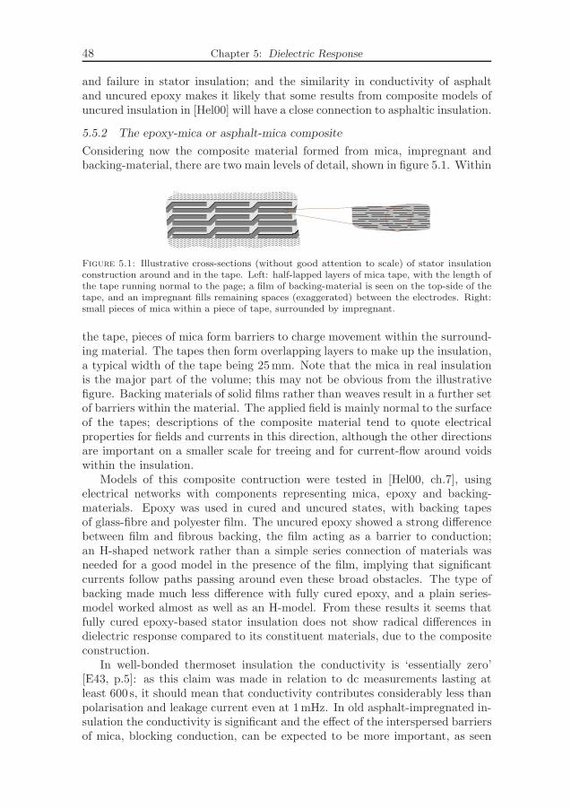
48 Chapter 5: Dielectric Response
and failure in stator insulation; and the similarity in conductivity of asphaltand uncured epoxy makes it likely that some results from composite models ofuncured insulation in [Hel00] will have a close connection to asphaltic insulation.
5.5.2 The epoxy-mica or asphalt-mica composite
Considering now the composite material formed from mica, impregnant andbacking-material, there are two main levels of detail, shown in figure 5.1. Within
Figure 5.1: Illustrative cross-sections (without good attention to scale) of stator insulationconstruction around and in the tape. Left: half-lapped layers of mica tape, with the length ofthe tape running normal to the page; a film of backing-material is seen on the top-side of thetape, and an impregnant fills remaining spaces (exaggerated) between the electrodes. Right:small pieces of mica within a piece of tape, surrounded by impregnant.
the tape, pieces of mica form barriers to charge movement within the surround-ing material. The tapes then form overlapping layers to make up the insulation,a typical width of the tape being 25mm. Note that the mica in real insulationis the major part of the volume; this may not be obvious from the illustrativefigure. Backing materials of solid films rather than weaves result in a further setof barriers within the material. The applied field is mainly normal to the surfaceof the tapes; descriptions of the composite material tend to quote electricalproperties for fields and currents in this direction, although the other directionsare important on a smaller scale for treeing and for current-flow around voidswithin the insulation.
Models of this composite contruction were tested in [Hel00, ch.7], usingelectrical networks with components representing mica, epoxy and backing-materials. Epoxy was used in cured and uncured states, with backing tapesof glass-fibre and polyester film. The uncured epoxy showed a strong differencebetween film and fibrous backing, the film acting as a barrier to conduction;an H-shaped network rather than a simple series connection of materials wasneeded for a good model in the presence of the film, implying that significantcurrents follow paths passing around even these broad obstacles. The type ofbacking made much less difference with fully cured epoxy, and a plain series-model worked almost as well as an H-model. From these results it seems thatfully cured epoxy-based stator insulation does not show radical differences indielectric response compared to its constituent materials, due to the compositeconstruction.
In well-bonded thermoset insulation the conductivity is ‘essentially zero’[E43, p.5]: as this claim was made in relation to dc measurements lasting atleast 600 s, it should mean that conductivity contributes considerably less thanpolarisation and leakage current even at 1mHz. In old asphalt-impregnated in-sulation the conductivity is significant and the effect of the interspersed barriersof mica, blocking conduction, can be expected to be more important, as seen

5.5.3 Currents in a healthy stator insulation system 49
for the uncured epoxy in [Hel00]; in [E43] the hygroscopic cotton backing tapesused before about 1970 are claimed to contribute to the conductivity.
The relaxation approximates a power law over the frequency range of power-frequency to millihertz at room temperature. This can be seen in tan δ for fullycured epoxy-mica insulation in [Hel00, ch.6]. The power law is widely assumedfor the polarisation current in time-domain measurements on stator insulation[E43], implying power law of the polarisation in frequency too [s.5.3]. Theresponse to a step-voltage V can be expressed as ipol(t) = C0V Kt−n, whereK is called the absorption coefficient (absorption is often used, in time-domainwork on machines, to mean general polarisation including dipolar and interfacialmechanisms). Estimated K and n values based on measurements from times of60 s, 190 s and 600 s on several examples of the main types of stator insulation areshown in [McD00]. For asphalt-based insulation n ∼ 0.8, and for the polyestersand epoxies n ∼ 1.0, both of these with about ± 20% variation between machinesand different occasions, taking the exponent well beyond a fractional power forsome values. Variation in K was as much as a factor of four between occasions,and values were generally more than ten times greater for asphalt than forpolyester or epoxy.
Taking the above results together with some practically oriented claims fromstandards, modern stator insulation in good condition can be said to have a asimple dielectric response over the frequency-range of interest in this work, anda low conductivity such that the displacement currents are dominant even at thelower range of frequencies relevant to the diagnostic methods considered in thiswork. The power-frequency relative permittivity is about 4 and a typical loss-tangent is about 0.5% [Sto04, p.250], in contrast to about 3% to 5% for asphalt-mica [Sto04, p.257]. Measurements made on newly manufactured epoxy-micastator bars in this work [s.18.3] gave quite similar values, with a power-lawexponent n ≃ 0.86.
5.5.3 Currents in a healthy stator insulation system
The above discussion covers only the relatively simple matter of a compositematerial between a pair of parallel electrodes. There are plenty of other sourcesof the current that flows during measurements of the electrical properties ofstator insulation. The main paths of current in the insulation are shown infigure 5.2 and described in the following paragraphs. The upper bar in thefigure is a ‘good’ one, in which the normal sources of currents are shown. Thelower bar is a remarkably bad one, and the diagram shows the main ways inwhich deterioration of insulation can change the currents flowing in the pathsfound in good insulation or can add further paths. These effects of deteriorationare examined in the following subsections.
In a stator insulation system in good condition the current flowing betweenthe conductor and earth is due mainly to the capacitance of the insulation withinthe slot. The symbolic capacitor representing this insulation in the diagram isthe frequency-dependent complex-capacitance due to the prompt response andpolarisation of the composite insulation material described above. A resistancehas been added, parenthesised, as a component that might be significant in

50 Chapter 5: Dielectric Response
( )
+− +− +−
slot−semicon contact worn gradingbreaks in stress−grading
crackedinsulation
poor earthing of
delamination
grading
bar surfaceabsorbed
water
earthed core
HV conductor
insulation
support−block
surfacecontamination
a Bad bar
a Good bar
thermally degraded,many small voids
Figure 5.2: Sources of current in the overall DR behaviour of stator insulation. Thisillustrative example uses a cross-section of two adjacent bars from a little way into the slotand a little way outside; figure 2.2 puts this into context for a relatively small high-voltagemotor.
asphaltic insulation but that should be negligible within epoxy-based insulationin good condition.
In the transition between the core and end-winding the nonlinear resistivestress-grading layer across the insulation surface forms a composite dielectricsystem whose current includes capacitance and loss components and harmonics,all dependent on the amplitude and frequency of the applied voltage; this isanalysed in much more detail in chapter 19.
Out in the end-winding region there will be very little current between theconductor and earth if adjacent bars’ conductors have the same potential; ifadjacent bars are on different phases and a diagnostic measurement is madewith one phase excited and others earthed, there will be capacitive couplingthrough the air and solid insulation.
5.5.4 Chemical changes in the insulation
The organic part of the insulation, mainly the epoxy, polyester or asphalt,changes chemically over time. Thermal aging [s.3.2.1] in an air-cooled machineresults in oxidation of the polymeric insulation material, which tends to increasethe number of polar groups, increasing the loss [Sto04, p.255]. The capacitancemay fall in spite of more polar gorups, due to voids and insulation expansionthat arise from the weakening of the insulation by thermal aging.
Some attempts have been made to obtain diagnostic information from in-ferences about these materials based on measurements on the whole winding.Stator insulation systems make this difficult, with their dielectric response hav-ing so many other effects than just those of the organic solid; on the other
5.5.5 Voids and insulation-expansion 51
hand the decomposition of this solid during the insulation’s lifetime is consider-ably more than would be tolerable in pure dielectrics such as polymeric cable-insulation. In [Dac89] the space-charge accumulation at mica barriers due toionic and electronic conduction mechanisms in epoxy has been considered as anexplanation of some of the time-dependence of current in stator insulation andas a guide to the degree of thermal aging. Greater aging is assumed to increasethe ionic mobility for conduction, due to ‘de-structuring’ of the polymer, andto decrease the electronic mobility for conduction, due to deeper traps. Thetime-constants of these mechanisms are different, and the degree of aging isinferred from the dominant time-constant in the current due to a dc voltageheld for many minutes. Capacitance measured at stages of accelerated thermalaging has been seen to have an initial fall from post-polymerisation (completionof curing) then a rise with a peak after considerable aging [Gof98].
5.5.5 Voids and insulation-expansion
As a result of thermal aging the epoxy or asphalt may be weak or largely missingfrom some parts of the insulation. Severely aged insulation is quite soft, withmany small voids (cavities) between poorly bound pieces of mica and aroundedges or wrinkles in the tapes. The substitution of gas for solid epoxy willincrease the capacitance of the bulk of the insulation even if the total volumebetween the electrodes is fixed. Slight extra expansion at the cooling ductsallows the electrodes of the inner conductors and slot semiconductor layer tomove further from each other, reducing the capacitance still further. About a1% decrease in capacitance can be expected due to the voids that arise from‘considerable’ thermal aging of epoxy-mica insulation [Sto04, p.250].
Discharges across the cavities at high voltage serve, as a first approximation,to short the cavities and thereby increase the capacitance as well as increasingthe loss. Slightly conducting surfaces in the cavities allow currents that thecavities, giving increased capacitance and introducing a dielectric loss due tothe energy lost in the resistance. In contrast to PD across the void, theconductivity could have effect even at low fields. PD activity is a likely causeof surfaces becoming more conductive (chapter 7). The effect of conductionon void surfaces is considered in [Gof78] as a way of explaining some of thevariation of capacitance and loss with voltage amplitude and degree of aging,for which simple PD models alone are not sufficient.
Within the main insulation there may be substantial delaminations; wide,shallow voids between tape-layers or between tapes and electrodes. At moderateapplied voltage these will block any conduction in the gap, and will reducethe insulation’s capacitance by adding a series gas-capacitor; the situation isqualitatively similar to the smaller cavities already mentioned. The relativelylarge area of a delamination normal to the applied field, and the consequentlarge ratio of the displacement current across the delamination to the length ofthe delamination walls that might have some conductivity to bypass the delam-ination, result in some quantitative differences. PD can be of large magnitudeand cannot so easily be avoided by slight conductivity of the dielectric surfaces.At low fields a given surface conductivity will not short-circuit the delaminationso effectively as it would short-circuit a smaller void.

52 Chapter 5: Dielectric Response
5.5.6 Electrostatic compression
A further effect on dielectric response from the voids and softening of thermallyaged insulation is due to electric-field-induced compression of the insulationbetween the electrodes. A simple model would expect compressive forces inproportion to the square of the applied voltage, resulting in an increased capac-itance at increased voltage even in the absence of PD. Odd-harmonic currentswill be caused by the changes of capacitance within each half-cycle.
This has been studied in [Bur88], including measurements on thermally agedstator bars of both types of impregnant, asphalt and epoxy. At 7 kV in barsrated about 20 kV with insulation thickness of 6 mm, a displacement of 0.1µmwas seen in the epoxy type and 0.5µm in the asphalt type; the field in theepoxy was taken high enough to get 0.5µm there too at 18 kV. Displacementincreased with lower frequencies. Variation of capacitance, ∆C, around thelow-field value of about 480pF was measured at voltages below PD inception,at 120Hz, 12Hz and 1Hz. The variation was seen to be several picocoulombs,fitting better with a model based on solid insulation moving to fill a delaminationthan with a model predicting smaller changes of capacitance based on uniformcompression of a solid with many small voids. Much larger ∆C, by some seventimes, was seen at the lowest than at the highest frequency; as the measureddisplacements did not change this much, one might wonder whether for examplesurface conductivity is playing a part. A suggestion of [Bur88] was the use ofthis variation of capacitance as a measure of delamination, possibly measuringthe response to a small ac voltage superimposed on a large dc voltage.
The study of voltage-dependence due to mechanical effects was taken furtherin [Pin91], with an analysis of effects of compression on capacitance, loss andharmonics, and several measurements on a complete stator winding. This wind-ing was in a micafolium-insulated 6.6kV motor with severe delaminations. Itwas measured at power-frequency at voltages below the (detected) PD inceptionof 3.3 kV; this old insulation system had fortunately no end-winding grading todisturb the results. The variation in capacitance was 60 pF within the totalcapacitance of 50 nF, with a quite good fit to ∆C ∝ V 2. The variation in tan δwas some 2.4% of the initial value of about 0.06. The third-harmonic currentwas also measured, and was seen to increase by a factor of three between 1 kVand 3 kV; unfortunately the absolute value is not reported. The tan δ and third-harmonic variations also fitted well to the square of the voltage.
5.5.7 Poor earthing of the bar surfaces
The outer surface of the main insulation is ideally held at earth potential bythe presence of a semiconductor layer in good contact with the core. A wornsemiconductor, or a poor contact with the core requiring currents from theinsulation to flow far along the semiconductor, will introduce a further resistancein series with the insulation’s capacitance, introducing a frequency-dependentloss. In extreme cases of practically no conductivity on part of the bar-surface,there will either be a straightforward reduction in measured capacitance, or athigh enough voltages PD will perform the task of conducting the displacement

5.5.8 Water absorption 53
current away, permitting some of the insulation capacitance to be measured butintroducing losses.
The change of the stator’s dielectric response due to lack of earth potentialaround the bar can be estimated for some simple cases. The effect will bestronger at higher frequencies where the series capacitance of the insulationhas a lower impedance. If the bar has lost contact with the core, and the slotsemiconductor is missing over an area of larger size than the insulation thickness,the situation described earlier for a delamination is a good approximation,reducing the total capacitance by introducing the further series capacitance ofthe gas-gap. If a significant length of the bar must be travelled by the currentin the slot-semiconductor before good contact with the core is made, then the‘linear distributed’ model of end-winding grading discussed in section 19.4 isrelevant. This could even be relevant for the length of bar within a coolingduct, if the semiconductor had an excessively low conductivity.
5.5.8 Water absorption
Water is highly polar, having by itself a relative permittivity of about 80 atthe frequencies of interest here. It also introduces some ions that can forma conduction current. Water absorption will therefore increase the capacitanceand loss of the insulation. Old thermoplastic insulation is hygroscopic [E43, p.9],so is rapidly affected. Modern insulation is very resistant to water absorption,but it is possible, particularly with direct water-cooled windings, for a slow, long-term presence of water to permeate through the whole thickness of insulation in amatter of years. The capacitance measured at power frequency may be increasedby some 5% by ‘significant’ water absorption [Sto04, p.252]; the presence ofwater is described by [E43] as ‘greatly affecting’ the permittivity.
The phenomenon of electroendosmosis can result in polarity-dependence ofthe current in the insulation [E43]; the current measured after many seconds ata high dc voltage is then typically ‘much higher’ when the winding’s conductorsare negative with respect to the core than when they are positive. Even-orderharmonics are therefore to be expected in the insulation system’s current at lowfrequency in this case.
5.5.9 Surface contamination
If the end-winding surface is contaminated with a somewhat conductive layer,such as of dust and condensation, a distributed circuit is formed from theshunt insulation-capacitance and series surface-resistance, rather like the stress-grading. The conductivity may be very varied between different points, andrather nonlinear with electric field; dry-bands and discharges across them mayform as is common on other contaminated insulator surfaces [LaF82]. Dis-placement currents through the end-winding insulation can be carried along thecontaminated insulation surfaces: the main destinations are the earthed core orthe surfaces of end-windings of other phases, reached through contamination onsupport blocking and lashing.
54 Chapter 5: Dielectric Response
5.5.10 Fractures and pinholes
Cracks and holes in the insulation, ultimately permitting a mildly conductivepath from the internal conductor onto the insulation surface, are most commonin the end-winding region [s.2.2.2]. In this case there may be a significantlyconductive path all the way between high-voltage and earthed conductors, otherthan just the bulk insulation’s conductivity that is so low for modern insulation.Removing the presence of a pure series capacitance removes the limit to thecharge that can move per cycle; a conductive path will show increasing charge,and therefore capacitance, with decreasing frequency. This situation’s sustainedconductive path is in contrast to all of the previously mentioned current-sources,apart from the possibility of surface-leakage at the winding terminals. Increasedtemperature may reduce the conduction in cracks [E95], presumably due tothermal expansion closing the crack or to less condensation; other conductionis increased.
5.5.11 Summary
Defects in the stress-grading, other than surface contamination, tend to reducethe current into the core. Worn grading or broken contact at the contact betweenslot semiconductor and end-grading are shown in the figure. Discharges, as witha delamination, may help to reduce the amount of ‘lost’ current due to suchbreaks.
The relevance of all these types of deterioration and their effect on the ap-parent DR of the insulation system is the desire to find indications of particularsorts of deterioration from the measurements. The above discussion of differentforms of deterioration gives very little obvious help: some forms decreasedthe capacitance, and some increased it; some had a nonlinearity or frequency-dependence, but so do end-winding grading systems. Cracks permitting a fullpath between the high-voltage conductor and earth without series capacitancehave probably the most distinctive result, but even this depends on a significantconductivity in the crack. The identification of a small change in permittivity ina small part of the insulation is hopelessly unrealistic; deterioration that affectsmost of the insulation or has a very severe local effect may be detected.
Chapter 6
Dielectric Response measurement
Currents flow in the electrodes of an insulation system due to the phenomena ofconduction and polarisation described in the previous chapter. These currentsare measured in material studies and in several common diagnostic methods.There are dynamic effects due to the pure material dielectric response and due toarrangements of different materials in complicated insulation systems: measure-ments made over a range of time or frequency permit some of the dynamics to beseen. Some common methods of dielectric response measurement are describedin this chapter, with a focus on instrumentation and interpretation of the typeof frequency-domain measurement used in this work. Common applications todiagnostic measurements on high-voltage insulation are described, consideringstator insulation in particular.
6.1 Dielectric-response measurements in time and frequency
A measurement at the low frequencies of interest here involves circuit propertiesat electrodes. Most commonly, a specified voltage-signal v(t) is applied, and thecurrent i(t) that this voltage causes in the dielectric is measured; from these thedielectric response is derived.
Calculation of some material properties requires further information aboutthe arrangement of electrodes and dielectrics, which for simple homogeneouscases can be expressed as the geometric capacitance C0. For measurements oncomplicated insulation systems it may be that the apparent dielectric responseof the whole system is all that is needed, perhaps for comparison with otherresults, or it may be that a property of a constituent material is to be inferred.In the following sections it will be assumed that the circuit properties betweenelectrodes are the ‘dielectric response’ to be measured.
The two common descriptions of material dielectric response [s.5.2] are thedielectric response function f(t) and the susceptibility χ(ω) [s.5.3]. The choiceof suitable v(t) to give easy calculation of one or the other of these functionsdefines the measurement as being time-domain or frequency-domain. The choiceof v(t) also affects the extent to which the prompt response ε∞ and conductivityσ can be distinguished from the polarisation, other than by further assumptionsand calculations [s.5.2].
Measurements that study dielectric response as a function of frequency aredielectric spectroscopy, DS. The obvious way of doing this is a frequency-domainmeasurement, FDDS, but sometimes a time-domain measurement is made andthen transformed into a function of frequency, in TDDS.
55

56 Chapter 6: Dielectric Response measurement
6.1.1 Time-domain measurements
The most obvious time-domain method is the response to a step-voltage. If thevoltage v(t) consists of a step V∆, with constant values before and after this,then the current due to polarisation after the step is ipol(t) = V∆C0f(t). Addedto this is the pulse of current carrying a charge V∆ε∞C0/ε0 to the promptcapacitance at the time of the step, and the current due to steady conduction,icon(t) = (v(t−) + V∆)σC0/ε0, where v(t−) is the voltage before the step.
A virtue of stepped voltage when interested in the dynamic polarisationis that the prompt response is absent from all but the short time around thestep, leaving the polarisation dynamics more clearly seen. The lower limit oftime-resolution is governed by how quickly the voltage on the test-object can bechanged and how accurately the times of measurements can be related to thisstep. With power-electronic switching of measurements on material samples thetimes can be submicrosecond [Jon96, p.269], but for high-voltage measurementson insulation systems the charging may take in the order of seconds for areasonable size of voltage-source. Noise-rejection of a single measurement islow compared to frequency-domain methods that can be tuned to an expectedfrequency, but a time-domain measurement obtains results corresponding to arange of frequencies from a single set of time-points, and the results can beaveraged over several repetitions of the measurement to reduce noise.
A common type of step-response measurement is polarisation and depo-larisation currents, PDC. The initial step is the connection of a dc voltage-source to a test-object that has previously been at zero voltage for a long time;after the initial transient the polarisation and conduction currents are measureduntil a time when the voltage source is replaced with a short circuit, and thedepolarisation current, in other words the polarisation current for a negativestep, is measured.
The results are only valid for measurements much shorter than the time forwhich the preceding voltage was held, as the direct relation of (de)polarisationcurrent to dielectric response function requires the initial state to be fullyrelaxed to the pre-step voltage. A common suggestion for acceptable resultsis a polarisation-time ten times as long as the measurement of depolarisationcurrent; a similar condition is assumed for the short-circuit time before the po-larisation. Some effects of a non-relaxed pre-step state may also be analyticallycompensated, given knowledge of the earlier voltages.
An advantage of PDC over a single step is that the steps of opposite directionshould result in the depolarisation currents being the negation of the polarisationcurrents; the conduction current can then be estimated from their sum. ForDS measurements on high-voltage insulation this appears to be widely held asan acceptable method of separating conduction and polarisation currents; butaccording to [Jon96, p.8], concerned with the detailed study of materials over awide range of times, the difference between the polarisation and depolarisationcurrent magnitudes does not give the constant value of these simple models.
Another form of time-domain measurement uses a ramped voltage: thesimple model of ε∞, σ and f(t) then gives a constant current from the prompt-response, a ramp from conductivity and a messy convolution from the dielectric

6.1.2 Frequency-domain measurements 57
response function. This form of voltage is more easily justified for industrialinsulation-testing [s.6.4.3] than for studies of dielectric response of materials:the ramp can reach voltages that stress the insulation considerably, but thegradual increase gives a chance of stopping if alarming trends in current areseen.
6.1.2 Frequency-domain measurements
The simplest frequency-domain measurement applies a sinusoidal voltage V (ω)as excitation, and measures the sinusoidal current I(ω) that flows. The conceptof functions of frequency implies that these signals extend forever in time, orin a practical sense that an equilibrium response to sinusoidal excitation hasbeen reached [s.16.3]. Given a linear object and an instrument without suchproblems as decaying terms in its feedback [s.6.2], a single cycle should suffice,although more may be needed to reduce the effect of noise; less ideal situationsmay require a few cycles of excitation before the current is measured.
The measured complex capacitance is then
C(ω) = C′(ω) − iC′′(ω) =I(ω)
iωV (ω), (6.1)
which in contrast to the pure complex capacitance of (5.7) includes the effectsof conductivity in its imaginary part. For an arrangement of electrodes withgeometric capacitance C0, surrounded by a material of permittivity ε accordingto (5.6) and of constant conductivity σ, the complex capacitance relates to thepolarisation, prompt response and conductivity as
C(ω) = C′(ω) − iC′′(ω) = C0
[
ε∞ε0
+ χ′(ω) − iχ′′(ω) − iσ
ωε0
]
=C0
ε0[ε∞ + ∆ε′(ω) − iε′′(ω) − iσ/ω]
= (C∞ + ∆C′(ω)) − i(
C′′pol(ω) + G/ω
)
, (6.2)
where C′′pol is subscripted to distinguish it as the pure C′′ due to polarisation
(5.6) rather than the measured C′′ (6.1). In the later practical uses it is themeasured values that are used, with any conduction term G included in C′′.
Other representations such as complex conductance may be useful in someapplications. The behaviour of high-voltage insulation systems will howevergenerally be closer to that of a capacitor, with the charge-per-cycle varying muchless with frequency than the charge-per-second does. The complex capacitancetherefore makes the material’s frequency-dependence clearer.
The last form of (6.2) is the most useful for a measurement on a wholeapparatus, where material properties are not the focus and where geometricdetails may not be known. It is clear that the currents due to the promptresponse and conduction will be unavoidably mixed with the currents due topolarisation. Given that both of these extra currents are frequency-independentit is possible to use the Kramers-Kronig relations [s.5.2] to calculate the purepolarisation components from the changes in the complementary parts. This

58 Chapter 6: Dielectric Response measurement
is used more in materials studies than when analysing the mixture of currentsources found in a stator insulation system.
Knowledge of the expected frequency of the current in FDDS permits tightfiltering to reduce noise, but a separate measurement is needed for each fre-quency. This is time-consuming at low frequencies such as the millihertz range,and several cycles are needed at each frequency if a strong advantage is to begained from the ability to filter the signal [s.6.4].
An overview of measurement methods used in the study of materials is givenin [Jon96, ch.10], from about twenty years ago. The classic bridge methods wereused down to about 10Hz, or even to 0.1Hz with clever use of xy traces on anoscilloscope. The availability of frequency-response analysers, FRA , in about1980 enabled measurements down to 10−4 Hz or 10−5 Hz, using an analoguecorrelator to compare measurements of the voltage and current on the test-object, with an electrometer as the input stage for measuring the current. TheDS instrument used in this work, described in chapter 9, can be seen as adigitally based FRA that includes the necessary electrometer and feedback.
6.2 Some practicalities of FDDS measurements
This section considers some general features of FDDS measurements using afeedback electrometer to convert the small current to a measurable voltage,then extracting the Fourier components of this current. More specific details ofthe instrument used in this work are found in chapter 9.
6.2.1 Input signals
A good insulator excited at a low frequency gives a very small current. Alaboratory sample may be only some tens of picofarads, which for applied voltageof tens of volts and frequencies in the millihertz range corresponds to a currentof picoamps. Industrial insulation systems will usually have higher capacitance,such as hundreds of nanofarads for a stator winding, and may also be testedat high voltages; the current can then come into the order of amps, but thepower-supply of the instrument [s.9.1.2] may have a lower limit.
Measurement of the small currents requires an input stage between the veryhigh-impedance test-object and the relatively low input-impedance of the FRAor analogue-digital converter that is used as the recording instrument; an elec-trometer provides a suitable interface. The instrument called an electrometeris a ‘highly refined dc multimeter’ [Kei04] specialised in measuring very lowcurrents, down to a few femtoamps, and voltages from very high-impedancesources; at the core of the electrometer instrument is a pure electrometer, whichcan be regarded as an op-amp optimised for very small currents. The inputstage for measuring current in FDDS uses such an electrometer in feedbackmode [Jon96, ch.10] with feedback components selected so that the expectedinput current will produce an output voltage within a reasonable range for therecording instrument. The feedback components have to be variable over a widerange of impedances, to allow for the range of test-objects that may be used andthe range of amplitudes and frequencies of the voltage applied to them; considerthe above examples ranging from picoamps to amps.
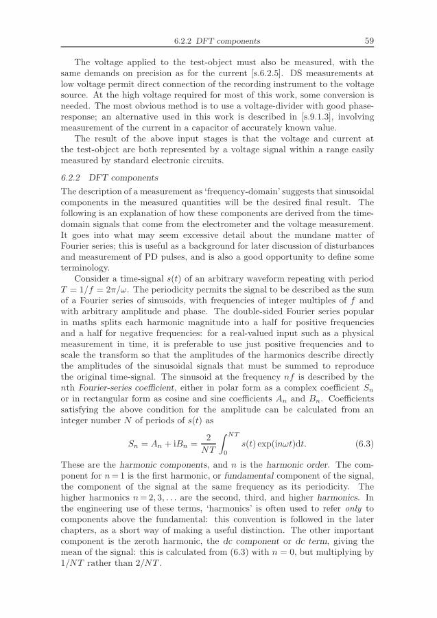
6.2.2 DFT components 59
The voltage applied to the test-object must also be measured, with thesame demands on precision as for the current [s.6.2.5]. DS measurements atlow voltage permit direct connection of the recording instrument to the voltagesource. At the high voltage required for most of this work, some conversion isneeded. The most obvious method is to use a voltage-divider with good phase-response; an alternative used in this work is described in [s.9.1.3], involvingmeasurement of the current in a capacitor of accurately known value.
The result of the above input stages is that the voltage and current atthe test-object are both represented by a voltage signal within a range easilymeasured by standard electronic circuits.
6.2.2 DFT components
The description of a measurement as ‘frequency-domain’ suggests that sinusoidalcomponents in the measured quantities will be the desired final result. Thefollowing is an explanation of how these components are derived from the time-domain signals that come from the electrometer and the voltage measurement.It goes into what may seem excessive detail about the mundane matter ofFourier series; this is useful as a background for later discussion of disturbancesand measurement of PD pulses, and is also a good opportunity to define someterminology.
Consider a time-signal s(t) of an arbitrary waveform repeating with periodT = 1/f = 2π/ω. The periodicity permits the signal to be described as the sumof a Fourier series of sinusoids, with frequencies of integer multiples of f andwith arbitrary amplitude and phase. The double-sided Fourier series popularin maths splits each harmonic magnitude into a half for positive frequenciesand a half for negative frequencies: for a real-valued input such as a physicalmeasurement in time, it is preferable to use just positive frequencies and toscale the transform so that the amplitudes of the harmonics describe directlythe amplitudes of the sinusoidal signals that must be summed to reproducethe original time-signal. The sinusoid at the frequency nf is described by thenth Fourier-series coefficient, either in polar form as a complex coefficient Sn
or in rectangular form as cosine and sine coefficients An and Bn. Coefficientssatisfying the above condition for the amplitude can be calculated from aninteger number N of periods of s(t) as
Sn = An + iBn =2
NT
∫ NT
0
s(t) exp(inωt)dt. (6.3)
These are the harmonic components, and n is the harmonic order. The com-ponent for n = 1 is the first harmonic, or fundamental component of the signal,the component of the signal at the same frequency as its periodicity. Thehigher harmonics n = 2, 3, . . . are the second, third, and higher harmonics. Inthe engineering use of these terms, ‘harmonics’ is often used to refer only tocomponents above the fundamental: this convention is followed in the laterchapters, as a short way of making a useful distinction. The other importantcomponent is the zeroth harmonic, the dc component or dc term, giving themean of the signal: this is calculated from (6.3) with n = 0, but multiplying by1/NT rather than 2/NT .
60 Chapter 6: Dielectric Response measurement
In the ideal case, s(t) is truly periodic with period T , and (6.3) is calculatedperfectly: there is no difference between using one or more periods, and theorthogonality of sinusoids of different frequencies ensures that only the compo-nent of s(t) at the frequency nf appears in Sn. In some calculations of Sn frommeasured data there may be a trouble of not knowing exactly the frequencyof the periodicity, and therefore having an error in the ω in the exponentialof (6.3); this is not a problem with DS as long as a single reference sourcecan be used to generate the voltage applied to the test object and to providethe signal corresponding to the exponential. In practical DS measurements thesignal s(t) can be expected to consist of a part that is periodic at the expectedfrequency, due to the known applied voltage, but there will also be componentsthat are aperiodic or that are periodic with a period other than T . The conditionof periodicity made for s(t) is then violated, and Sn can be affected even bya signal that would have no component at frequency nf if extended over alltime. The extent of this effect can be seen by solving (6.3) for the particulardisturbance.
There are several disturbance signals relevant to later discussions of DS. Aconstant ramp or decaying exponential may occur with particular combinationsof electrometer feedback [s.6.2.6] and measured current [s.6.2.7]. Pulses ofrandom noise may occur at some points in the signal, differing from PD chargesonly in that they are not expected to have periodicity; for infrequent PD oversmall numbers of cycles the distinction from noise is weak. High-frequency noisesuch as background radiated noise and thermal noise is filtered well from themeasurement of Sn, since it integrates close to zero over any small part of T .Sinusoids at frequencies quite similar to the measured frequencies may be pickedup from external sources: disturbances at the power frequency are particularlycommon [s.12.4]. A signal consisting only of a disturbance Md cos(2πfdt) resultsin an nth cosine-coefficient An of
An = Md sinc
(
2πNnf−fd
nf
)
, (6.4)
where sinc(x) ≡ sin(x)/x [Jon96, p.277]. A larger number of periods clearlygives better noise-rejection, but with local maxima and minima as the totaltime-window of NT passes multiples of the frequency difference f−nfd.
It can be seen from (6.3) that a measurement over N cycles gives thearithmetic mean values of the separate measurements over single cycles. Parts ofthe signal occurring only in some periods will appear as weaker signals occurringin all periods. Parts whose mean Sn over many periods tends to zero willbe better removed by including large numbers of periods, as was seen for thesinusoid at nonharmonic frequency. The larger number of periods is no help witha ramp: this can be decomposed into the sum of a zero-centred ramp, similarin each period, and a dc term that gets larger in each period; the effect on aparticular harmonic order other than the dc term is independent of the numberof periods used. A decaying exponential has a progressively lower decay, inabsolute terms, over subsequent periods, and only for this reason has a reducedeffect when more periods are used.

6.2.2 DFT components 61
The contributions of several functions of time on the fundamental componentS1 are shown in figure 6.1 for varied N . The sinusoid of frequency f and the
0 5 10 15 20 25 300
0.2
0.4
0.6
0.8
1
1.2
1.4
number of periods, N
mag
nitu
de, a
.u.
0 5 10 15 20 25 30−1
−0.5
0
0.5
1
number of periods, N
angl
e / π
rad
sin(ω t)
1
sin(0.90 ω t)
t
5 exp(−t)
Figure 6.1: Contributions of various time-functions to the 1st harmonic (fundamental-frequency) component S1 of equation (6.3) at f = 1Hz, for varied numbers of periods N .
dc signal are already pure harmonic components, so they give the expectedcontributions of 1 and 0 to the fundamental component, along with some nu-merical noise in the phase caused by the dc signal. The sinusoid at a 10%difference in frequency behaves according to (6.4); note that figure 6.1 showsthe magnitude of the complex coefficient, which changes only half as fast withN as the real part used in (6.4). The ramp and exponential give constant anddecaying magnitudes.
The correlator of the analogue type of FRA works directly on the inputvoltages representing voltage and current at the test-object. The current ismultiplied by sinusoids in phase and in quadrature with the voltage, whichideally is sinusoidal. These sinusoids are like the real and imaginary part of theexponential in (6.3), and the integrals over a whole number of cycles give therectangular-form coefficients An and Bn. Compensation for phase-shifts in thecircuit and feedback allows calculation of the complex capacitance by (6.1).
A more modern approach takes advantage of cheap commodity-hardwarethat can sample and process signals at for example rates of hundreds of kilohertzand resolutions of 16 bits. The input voltages representing voltage and currentat the test object are directly sampled and digitised, and signal processing is allon the digital side. The calculation by (6.3) of the nth Fourier series coefficientis replaced with a discretised version, the discrete Fourier transform (DFT),operating on K samples s[k] taken at regular intervals over N periods,
Sn =2
K
K−1∑
k=0
s[k] exp
(
i2πknN
K
)
, (6.5)
where again the dc term n = 0 is a special case for which the result of (6.5)must be halved. The similarity of Sn between (6.3) and (6.5) is dependent onthe sampling; the many samples per period of the instrument used in this work[s.9.1.6] make the approximation close.

62 Chapter 6: Dielectric Response measurement
The implementation of (6.5) requires for each sample s[k] the generationof numbers corresponding to the real and imaginary parts† of the exponentialterm; the product of each with s[k] is accumulated (summed with an existingvalue) into a variable for the real and for the imaginary part of Sn. The sameis done for several values of n: the instrument used in this work includes thecomponents from 0 to 8. The sampling must clearly be coordinated with theexpected periodicity of the signal: a small error such that the K samples ofsupposedly N cycles actually occur over a slightly different number of cyclesis the same as the error in ω already discussed for (6.1). The sampling musttherefore be locked to the generation of the output voltage, so as to guaranteemeasurements based on exactly the right fundamental frequency. Just as for theanalogue FRA, the results of Sn for the inputs representing voltage and currentmust be adjusted for effects of the electrometer circuits and external circuit, togive the desired frequency-domain results for the quantities at the test-object.
6.2.3 Distorted sources and nonlinear test-objects
The discussion of FDDS, up to this point, has described how the dc, fundamental-frequency and higher harmonic terms are measured for the voltage and currentat the test-object, but has only considered the use of capacitance and loss, bothof which relate only to the fundamental-frequency.
The voltage applied to the test-object surely has some level of distortion,a deviation from a pure sinusoid, meaning that not all the voltage harmonicsV2,3,... are nonzero. Even if the test-object is linear, the nth voltage harmonicVn will result in a nonzero nth current harmonic In. The capacitive nature ofa typical test-object will result in the amplitude of a current harmonic beingproportional to its harmonic order as well as to the amplitude of the respectivevoltage harmonic, so that similar amplitudes of V2 and V8 would give |I8| = 4|I2|.
With the amplifier and DS instrument used in this work [s.9.1.2], driving alargely linear load at 10 kV, the harmonic voltages are in the order of 1 V whenthe amplifier is giving a large proportion of its rated current, and much lower forsmall currents. Although these may sound small, the effect of voltage harmonicsoften needs to be removed before using the current harmonics in calculations.For delicate measurements of the contribution of small nonlinear sources tothe much larger total current in a capacitive object, even the currents due tothese small voltages can be significant. For measurements on strongly nonlinearobjects the strong current harmonics will cause extra voltage harmonics due tothe supply impedance, leading to further current harmonics in the capacitance.
Unless there is very high dispersion it is a reasonable first-approximation touse the capacitance C′ measured from the fundamental components of voltageand current to estimate the current harmonics inωVn(ω)C′ due to the measuredvoltage harmonics Vn(ω), and to compensate the original measured current In
for the effect of the voltage harmonics by subtract this estimate,
In(ω) = In(ω) − inωVn(ω)C′, n = 2, 3, . . . . (6.6)
† These are often called the DFT coefficients, but this name is avoided here as Sn is the(approximated) ‘Fourier series coefficient’, probably leading to some confusion.
6.2.4 Calculation of input current 63
The measurement of the harmonics is good enough that applying this compen-sation to the case of a very linear gas-capacitor reduces the current harmonicsby several times. Other methods than (6.6) may be preferable in certain cir-cumstances: complex capacitance can be used instead of pure capacitance, andthe frequency-dependence of capacitance can be modelled or measured to givea better estimate of the value at the harmonic frequency.
Nonlinearity of the test-object results in current harmonics even for a purelysinusoidal voltage. Several sources of nonlinearity in stator insulation havealready been mentioned in [s.5.5]. Most of the sources give a quite smoothnonlinearity, so that most of the information is in the first few harmonics. Evenfor the inherently pulse-like phenomenon of PD, the individual PD events in awhole stator are only a tiny part of the whole DS current, and aggregation ofthe many events that are needed to get a discernible measurement gives againa relatively smoothly distorted current where the harmonics beyond about thetenth are of very little importance.
The approximate time-signal s(t) formed from just the spectrum up to andincluding the Nth harmonic can be calculated from the DFT results Sn as
s(t) = ℜ[
N∑
n=0
|Sn| exp(
i (nωt − ∠Sn))
]
=
N∑
n=0
(
An cos(nωt) + Bn sin(nωt))
=
N∑
n=0
|Sn| cos (nωt − ∠Sn) , (6.7)
which is useful for physically based consideration of the shape of the currentfrom its fundamental and harmonic components. One useful purpose of havingthe DFT components rather than just working with time data directly is thatthe tight filtering of harmonics allows even very small nonlinear currents to bestudied against a background of a large fundamental component.
6.2.4 Calculation of input current
The circuit in figure 6.2 is an electrometer ‘EM’ with its feedback componentsRfb and Cfb The direction of components and signal is right-to-left in orderto be consistent with later diagrams of the whole measurement system, wherethe applied voltage goes left-to-right to the test object Cx, and the current ismeasured on its return to the instrument.
The input current I(ω) to the electrometer circuit needs to be calculatedfrom the measured electrometer output voltage Vo(ω). This would be a simpleop-amp problem if the electrometer were an ideal op-amp: in fact, its inputresistance and capacitance are finite, and its gain H(ω) is finite, complex andfrequency-dependent. The approximate values of the electrometer parametersin the instrument used in this work are given in section 9.1.5. For very accuratecalibration the values of feedback components may also need to be modelled asfunctions of frequency.

64 Chapter 6: Dielectric Response measurement
signal earth
+EM
Vhv(ω)
Ifb(ω)
Cs Rs
Vi(ω)
CxCfb
Rfb
Vo(ω)
I(ω)+H(ω)+
−
Figure 6.2: Circuit diagram of electrometer feedback, test-object, and parasitic components,for analysis of the relation between output voltage and input current.
The shunt components Rs and Cs in the figure can include the connections tothe test object and the electrometer input. Note that if the electrometer’s gainwere perfect, always holding its inverting input to the signal earth potential,then the shunt components would be irrelevant. For measurements with longleads, high frequencies or large test-objects the series impedance of leads mayneed to be modelled too.
The resulting relation of current at the input to measured voltage at theoutput is
I(ω)
Vo(ω)= −
[(
1
Rfb+ iωCfb
)
+1
H(ω)
(
1
Rfb+ iωCfb +
1
Rs+ iωCs
)]
(6.8)
The first term here, involving the feedback components, is the ‘ideal’ relation ifthe electrometer had a perfectly high gain so that its inverting input would be atrue virtual earth. The further terms with the factor 1/H are the consequenceof the inverting-input’s node not being at true signal earth potential, causingthe feedback voltage to change and some of the input current to be shuntedaway from the feedback components.
6.2.5 Error sensitivity
There are errors in the measurement of magnitude and phase of the voltageand current at the terminals of a test-object; these come from calibration errorsin feedback components, circuit elements not perfectly modelled, temperature-dependence of calibration, and more. Relative errors in magnitude and absoluteerrors in phase contribute similarly to the errors of complex capacitance, as canbe seen by considering (6.1) and de Moivre’s theorem.
Dielectric measurements are generally concerned with the components ofcurrent in phase and in quadrature with the voltage, corresponding to loss andcapacitance. In a low-loss dielectric such as most high-voltage insulation, theratio of these components, tan δ, can be very low, in the order of 10−5 in somepolymers. With this huge difference in relative sizes, even a 10 microradianphase error will be a 100% error in C′′. The effect of magnitude errors is muchless severe, resulting in a similar relative error in C′ and in C′′.
The calibration and modelling of components of the instrument and theexternal circuit must therefore be done very carefully. Modelling of, for example,

6.2.6 Choice of feedback 65
an extra filter would need to be very confident of limits of variation of componentvalues with movement and temperature.
Stator insulation is actually not as critical as the above example, havingtypical power-frequency loss-tangents of significant fractions of a percent, forgood modern insulation at moderate voltage, and several percent for old insu-lation. It is nevertheless desirable that phase-errors be small, particularly forlaboratory work where detailed inferences may be desired from the data.
A further point about phase errors and feedback calibration is made in[Wer01a, p.47]. If a single feedback component is used, such as just a capacitor,it would need a phase error in itself in order to create a phase error in the result.When the feedback current is instead shared between a parallel capacitor andresistor, a relative error in magnitude in the value of one of the components willgive a phase error in the total feedback impedance that is used in calculating thecurrent. The effect is greatest when the components have similar impedance.This is just a further reason, beyond those in [s.6.2.7], for choosing one feedbackcomponent to be strongly dominant.
6.2.6 Choice of feedback
The electrometer output voltage, Vo in figure 6.2, is likely to have an optimallevel in the few-volt range of electronic circuits; this voltage across the feedbackcomponents must provide a current that matches the measured current. DSmeasurements generally are made over at least several decades of frequency, andthe capacitive test-object typical of high-voltage insulation will pass a currentlargely proportional to frequency. Measurements using resistive feedback there-fore require switching between several different feedback resistances in order tokeep the electrometer output voltage within its desired range; measurementsusing capacitive feedback can use a single capacitor over all the frequenciesunless the test-object is highly dispersive.
A disadvantage of capacitive feedback is that the total charge that can bepassed through the capacitor is limited by its capacitance and the range ofelectrometer output voltage. A test-object with significant conduction will passlarge amounts of charge per half-cycle at very low frequencies, which may be toomuch for a reasonable size of feedback capacitor to supply. There may be a dccomponent required in the feedback current, which would make it impossible tocontinue with capacitive feedback beyond the time taken for this current to pushthe electrometer output voltage to its limit. This dc component is necessaryif the test-object has polarity-dependent behaviour such as electroendosmosis[s.5.5.8] or an asymmetric external PD-source [s.7.2.1], or if interference iscoupled in from extraneous currents sharing part of the measurement circuit,or if the electrometer itself has a significant input offset current [Sed91, p.100].Resistive feedback permits a dc currents to be sustained for any time by aconstant electrometer output voltage. It also simplifies the relation of outputvoltage to measured current, making them directly proportional. Even if ameasurement is not run for long enough to drive the electrometer into overload,a dc current with capacitive feedback will result in a continual ramping of theelectrometer output voltage: if the ramp changes significantly within a cycle,this ramping will affect the DFT results for the sinusoidal components as well

66 Chapter 6: Dielectric Response measurement
as the dc term [s.6.2.2]. Resistive feedback would permit the true dc current tobe measured, and would not disturb the other DFT components.
A disadvantage of resistive feedback is seen when the measured currentcontains pulses of many times the mean amplitude of the signal; this is expectedin the case of a test-object that contains PD or poor connections, particularlyat low frequencies where the mean current is low. The feedback resistor willeither be so low as to give a poor signal to noise ratio when measuring thesignal between pulses, or will be so high that the electrometer voltage will hit itslimit (electrometer overload) during the large current-pulses. This disadvantagecomes from the same feature as was an advantage for dc currents: that is,the resistive feedback forms a proportional ‘transresistance’ amplifier, whilecapacitive feedback forms an integrator. A pulse of current into capacitivefeedback simply requires a step change in output voltage rather than a veryquick rise to high values.
The feedback should be kept mainly capacitive or mainly resistive, for rea-sons described in [s.6.2.5] and [s.6.2.7]. In this work the mainly resistive feedbackhas been preferred for several reasons: some test objects are expected to bepolarity-dependent, measurements are made at low frequencies and with lossyobjects such as those with external PD, and dc components are expected fromsome types of PD source. It has been seen that a small amount of capacitivefeedback can be sufficient to buffer sharp pulses while allowing the other benefitsof resistive feedback to be obtained; this is described further in chapter 14.
6.2.7 Feedback ratio
The description of some relative merits of resistive and capacitive feedback maymake a quite even mixture seem a good idea: this could provide a resistivebypass for dc currents, and a capacitive buffer to hold pulsed charges untilenough time has passed for them to leave through the feedback resistance.
In fact, a significantly mixed feedback has problems from output voltagewaveform as well as from the effects of feedback calibration errors that were men-tioned in section 6.2.5. Even with a linear test-object the previous, frequency-domain, analyses of the electrometer feedback circuit have problems. It is nottrue that a particular frequency has been present forever: the applied voltage isat some time turned on from zero or from an earlier value. Nor is it true thatthe output voltage is unlimited: even if the presence of a constant offset voltageon the output would not affect the measured fundamental-frequency value, itmay drive the electrometer output into overload.
The circuit of figure 6.3 is used for analysis of the effects of feedback com-ponents on transient response. The test-object is represented, at a particularfrequency, as a pure capacitance Cx and a parallel resistance Rx; the loss-angleδ = tan−1(1/ωCxRx) then gives the phase-lag of the current i(t) compared tothe case where Cx is a pure capacitance. The electrometer is treated as ideal:the supply and test-object therefore form an independent current-source i(t)into the virtual-earth node on the inverting input, and the feedback current
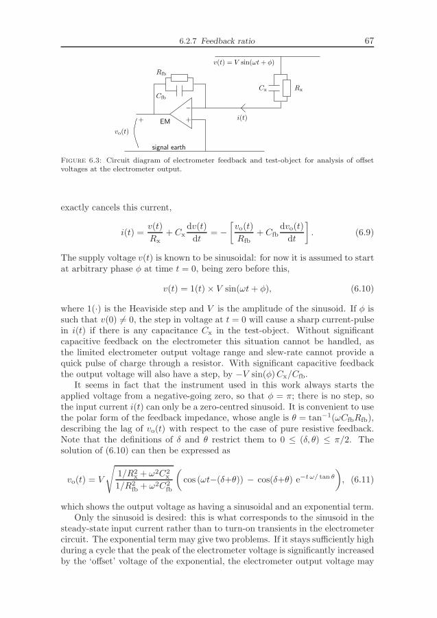
6.2.7 Feedback ratio 67
+
−
signal earth
+ EM
Cx Rx
Cfb
Rfb
vo(t)
i(t)
v(t) = V sin(ωt + φ)
Figure 6.3: Circuit diagram of electrometer feedback and test-object for analysis of offsetvoltages at the electrometer output.
exactly cancels this current,
i(t) =v(t)
Rx+ Cx
dv(t)
dt= −
[
vo(t)
Rfb+ Cfb
dvo(t)
dt
]
. (6.9)
The supply voltage v(t) is known to be sinusoidal: for now it is assumed to startat arbitrary phase φ at time t = 0, being zero before this,
v(t) = 1(t) × V sin(ωt + φ), (6.10)
where 1(·) is the Heaviside step and V is the amplitude of the sinusoid. If φ issuch that v(0) 6= 0, the step in voltage at t = 0 will cause a sharp current-pulsein i(t) if there is any capacitance Cx in the test-object. Without significantcapacitive feedback on the electrometer this situation cannot be handled, asthe limited electrometer output voltage range and slew-rate cannot provide aquick pulse of charge through a resistor. With significant capacitive feedbackthe output voltage will also have a step, by −V sin(φ)Cx/Cfb.
It seems in fact that the instrument used in this work always starts theapplied voltage from a negative-going zero, so that φ = π; there is no step, sothe input current i(t) can only be a zero-centred sinusoid. It is convenient to usethe polar form of the feedback impedance, whose angle is θ = tan−1(ωCfbRfb),describing the lag of vo(t) with respect to the case of pure resistive feedback.Note that the definitions of δ and θ restrict them to 0 ≤ (δ, θ) ≤ π/2. Thesolution of (6.10) can then be expressed as
vo(t) = V
√
1/R2x + ω2C2
x
1/R2fb + ω2C2
fb
(
cos (ωt−(δ+θ)) − cos(δ+θ) e−t ω/ tan θ
)
, (6.11)
which shows the output voltage as having a sinusoidal and an exponential term.Only the sinusoid is desired: this is what corresponds to the sinusoid in the
steady-state input current rather than to turn-on transients in the electrometercircuit. The exponential term may give two problems. If it stays sufficiently highduring a cycle that the peak of the electrometer voltage is significantly increasedby the ‘offset’ voltage of the exponential, the electrometer output voltage may
68 Chapter 6: Dielectric Response measurement
be pushed beyond its limit. If it decays slowly enough that it has not vanishedwithin a small part of the period of one of the measured DFT components,but quickly enough that there is a significant difference in its values betweena positive half-cycle and a negative half-cycle, it will contribute to that DFTcomponent, introducing an error in the measurement of the desired steady-stateperiodic current.
The best behaviour is for there to be no exponential term. This couldbe achieved by choosing θ so that δ+θ =π/2 to make the cosine term of theexponential become zero; this means making the test-object and feedback havethe same ratio of capacitive and resistive currents, in other words the same time-constants, similar to a good voltage-divider design! It could also be achievedby Cfb = 0, giving θ = 0, as is obvious from considering that pure resistivefeedback has no integrator-effect. A very quickly decaying exponential, muchquicker than a cycle, will also avoid the problems: this is possible if θ ≃ 0, whichimplies that the capacitive current in the feedback is only a small proportion ofthe total.
Alternatively, a very slow change in the exponential term will require con-sideration of maximum output voltage but will not disturb the DFT resultsignificantly. The slow decay is only possible, under the conditions that havebeen put on the parameters of (6.11), with strongly capacitive feedback, wheretan θ is very large and where the test-object is not also strongly capacitive whichwould make cos(δ + θ) be small. The peak value of electrometer output voltagecan be in the worst case twice as high as the peak of the sinusoidal component,but this requires dominantly capacitive feedback and a dominantly resistivetest-object.
The capacitive feedback ratio, CFBR, is a definition used within the programfor controlling the DS instrument used in this work: it is the proportion of thetotal feedback current that flows in the capacitive branch,
“CFBR” = ωCfb/√
1/R2fb + ω2C2
fb. (6.12)
Considering that most test-objects are mainly capacitive, the cases where feed-back is mainly resistive or mainly capacitive will not cause significant errorsin the result, and the offset voltage will in either case be small as long as theapplied voltage starts at zero. The CFBR should therefore be kept close to oneof its extreme values of 0 or 1 in order to keep mainly to resistive or capacitivefeedback. A variation of up to a few percent from these values is permissiblewithout severe effect on the results, particularly if letting some cycles of voltagebe applied before using the measurement.
6.3 DS measurements for general HV diagnostics
Insulation based on wood-pulp and petroleum is used in several important typesof high-voltage equipment: the insulation of transformers consists of paper andpressboard surrounded by oil, and the insulation of bushings and old powercables consists of paper impregnated with wax or oil. Water in the paperaccelerates decomposition of the cellulose, and this decomposition results inwater: the water content is therefore a useful quantity to measure for diagnostic

6.4 DS measurements on stator insulation 69
purposes, and water is fortunately easy to detect by dielectric measurementsas it is so polar. A transformer is a complex construction involving liquid andsolid insulation, so other effects such as oil conductivity are influential in themeasured result. Nevertheless dielectric spectroscopy methods in time and infrequency have been widely applied to the insulation of transformers [Gub03],with water content a particular interest. Voltages of just a few volts can be usedto good effect in frequency-domain measurements. Dielectric spectroscopy hasalso been used on paper-insulated cables [Nei04].
Cables with XLPE insulation have largely superseded the paper-insulatedones. Degradation by water-treeing was a large and wholly unanticipated prob-lem of this type of insulation, leaving early generations of cables from the 1960sand 1970s particularly vulnerable. Water has a strong effect on the dielectricresponse of a low-loss dielectric such as XLPE, although the relatively lowproportion of water trees in the total volume makes sensitive measurementsimportant. Frequency-domain dielectric spectroscopy has been extensively in-vestigated [Wer01b] [Wer01a, ch.4,5], including the use of varied high-voltageto stimulate the nonlinearity of water-treed insulation. The stress-gradingsometimes used at cable terminations and joints has strong similarities to theend-winding stress-grading considered in chapter 19, so it is a further source ofvoltage-dependence. These accessories make up only a small part of the totallength of cable, in contrast to the two winding-ends per metre or so of statorwinding, so their contribution to the total response is relatively weak.
6.4 DS measurements on stator insulation
No diagnostic measurement in common use on stator insulation can be seen ashaving a main interest in the dynamic response of the insulation material’spolarisation. Several commonly used measurements are strongly related toDS, and several approaches to purer DS measurements have been taken byresearchers.
6.4.1 Capacitance and loss
Measurements of capacitance and loss-tangent are widely used. In contrastto true spectroscopy the measurements are at just one frequency, usually thepower frequency for the sake of a simple voltage-source. Instruments for thesemeasurements typically use bridge methods [Kuf00, s.7.2], permitting relativeaccuracies of the order of 10−4 [Sto04, p.255]. The result is a total value forthe whole measured part of the winding, and the effects even of quite severeproblems can be small changes of the order of a percent: these types of mea-surements will only be sensitive to problems affecting a significant proportionof the insulation.
If the solid insulation-material is the focus, the voltage will be kept lowto reduce nonlinear contributions such as PD and surface-leakage. Used inthis way the measurement is moderately effective at detecting the increasedC-tan δ due to water absorption [s.5.5.8], and the decreased C′ due to voids[s.5.5.5] and increased tan δ due to oxidised polymer [s.5.5.4]. Changes duringmanufacture, as impregnant fills the gaps in the insulation and then is cured,are also sometimes tracked with low-voltage C-tan δ measurements.

70 Chapter 6: Dielectric Response measurement
The capacitance and loss measurements are often made at high voltages,sometimes well beyond the service stress; in these case PD is arguably themain interest. To give more information than just a single measurement at,for example, the rated voltage, it is normal to use several voltages, below andabove the expected inception level for PD; common values are 20% incrementsfrom 20% to 120% of the rated line-voltage, applied between a phase and earth.Advantage can then be taken of using relative values [s.4.6], by studying thevariation of C′ or tan δ between different voltage levels; the increase in thesequantities with voltage is called the tip-up. The common tan δ tip-up testcompares measurements at the several voltages, often plotting the change togive an idea of the extent of the PD activity and the voltage ranges in which itmost increases. Capacitance tip-up is sometimes measured too, more in Europethan in North America; the relative change in value is less than for tan δ, sincecavity PD tends to have quite similar absolute contributions to both of thesequantities and the absolute capacitance of the insulation is much greater thanthe loss. The main feature of the insulation that is measured by the tip-up is the‘void content’, on the assumption that a high enough voltage causes all voidsto be ‘shorted out’ by nonlinear effects such as PD. A reduction of tan δ withincreasing voltage, beyond a high value where much PD is occurring, is widelyreported [E286]; this has been studied in [Gof78], which considers the tip-up tohave a more complex description than simply more cavities breaking down.
Some examples of C-tan δ tip-up are given in figure 6.4. These are fromindustrial measurements made on 24 hydro-generators of rated power from10MVA to 250MVA, rated voltage mainly around 10 kV but up to 20 kV forthe largest powers. The machines are from several manufacturers and theirinsulation is mostly of epoxy-mica, the one exception being polyester-mica.Measurements have been made on phases separately then phases all together;the measurements on all together are shown by dashed rather than dotted linesbetween the measured points. The plots of relative C′ and of tan δ show arelative change of a few percent in C′ and C′′ with voltage.
6.4.2 Insulation ‘resistance’ and polarisation index, IR/PI
The measurement of insulation resistance, IR, is a primitive ‘polarisation-current’measurement [s.6.1.1] using one or a few time-points. A dc voltage is appliedbetween the conductor and earth, and the current that flows in the insulationsystem is measured at some later times. Instead of presenting the measuredcurrent directly, the ratio of the applied voltage to the current is taken, and isreferred to as a resistance although it is changing in time due to the polarisationterms in the current.
Times are generally at least 60 s, and commonly up to 600 s. The voltagesare not as high as the working level of ac, but are usually some kilovolts togive a chance of nonlinear conduction being seen. The results, as for C-tan δmeasurements, are totals for the whole measured part of the winding, whichreduces the sensitivity to a problem in a small part of the winding. However,the low bulk conductivity of thermoset insulation and the low polarisationcurrent after times of several minutes give a good chance of detecting the smallconduction path provided by a single fracture [s.5.5.10] or by water absorption.

6.4.2 Insulation ‘resistance’ and polarisation index, IR/PI 71
0.2 0.4 0.6 0.8 10
500
1000
1500
2000
2500
3000
3500
4000C
’ [n
F]
V / Vline
0.2 0.4 0.6 0.8 10
0.01
0.02
0.03
0.04
0.05
0.06
0.07
0.08
tan(
δ)
0.2 0.4 0.6 0.8 10.99
1
1.01
1.02
1.03
1.04
1.05
1.06
1.07
rela
tive
C’
0.2 0.4 0.6 0.8 1
1
2
3
4
5
6
rela
tive
tan(
δ)
Figure 6.4: Measured tip-up of capacitance C′ and loss-tangent tan δ on 24 hydro-generatorswith thermoset insulation, applying 0.2, 0.4, 0.6, 0.8, 1.0 of the rated line-voltage betweenphase and earth. Lines link points to clarify the trends: dashed lines show measurementsmade from all phases to earth, dotted lines single phases to earth.
A conduction path to the end-winding capacitance, due to surface contamination[s.5.5.9], can also be detected as unexpectedly high current even after manyseconds. Common criteria for minimum IR(60 s) are > 100MΩ for post-1970insulation and > (Un/1 kV + 1)MΩ for older insulation [E43]; good insulationmay commonly have many times higher values.
Conductivity is highly temperature-dependent [s.5.1]. IR measurements areconventionally given as values ‘corrected’ to 40 C, using an exponential depen-dence such that conductivity increases by a factor of 2 for an increase of 10 C.According to [Sto04, p.239] the correction factors simply ‘don’t work’, givingquite different corrected results from the same object at different temperatures.The conventional values are based on studies from the 1950s, but the change intemperature for a doubled conductivity has more recently been found to rangefrom 2 C to 20 C [E43, p.10].
Condensation on winding surfaces has strong effect [E43] on the surfaceconductivity, and the winding should be above the dew-point if the results areto be meaningful. Direct water-cooled windings should have the cooling waterremoved, or at least checked for low conductivity, so as not to upset the results[E43, p.12]; this would clearly be very important in making FDDS measurementsat low frequency, and is even mentioned in relation to power-frequency C-tan δ

72 Chapter 6: Dielectric Response measurement
measurements [E286, p.24].To make IR results less dependent on temperature and on knowledge of the
geometric capacitance, the ratio of IR values at two times can be used, to givethe polarisation index, PI. Ratios of the 10minute to 1minute IR values areoften used. For any mica-based insulation system likely to be found in service,a standard criterion is PI > 2.0 [E43]. A lower value suggests so little changebetween these two times that a significantly conductive element in the currentis likely. PI, or any IR based method, “only finds contamination and seriousdefects”; it is “excellent” at finding cracks, contamination and water-soaking[Sto04, p.238].
6.4.3 Less-common industrial methods
The simple dc hipot test [s.4.7] is a pure test of endurance, without measure-ment. By making a current measurement during this test, further informationcan be obtained, making it like a form of high-voltage polarisation-currentmeasurement. The applied voltage may be a single step, multiple steps or a ramp[Sto04, p.245]. The ramp test, including use at voltages of service rather thanhipot levels, is popular among some hydro-generator operators, particularly inNorth America [Rux04]. There has been recent work to standardise methods andspread information about the appearance of different defects in the measuredcurrent [E95], and to analyse the components in the current in comparison withstepped-voltage excitation [Dav06].

Chapter 7
Partial Discharges
This chapter introduces gas discharge mechanisms, situations in which partialdischarges arise, and the effect of the applied voltage’s frequency. The natureand effect of partial discharge in stator insulation systems is described based onliterature and industrial industrial measurements. Sources of partial dischargein stator insulation are described. Measurements of partial discharges are leftuntil chapter 8.
7.1 Gas discharges
The mechanisms of gas discharges (electrical discharges in gases) were widelyinvestigated during the late nineteenth and early twentieth century. They arethe usual starting point in discussing such apparently disparate phenomenaas partial discharge, lightning and other long discharges, and liquid and solidbreakdown [Kuf00, ch.6]; of these, partial discharge and solid breakdown are ofmost interest in studies of stator insulation.
Just the details most relevant to later discussion of PD are now given; a lotmore than this is needed in order to get a good grasp of the subject. Use ofseveral sources is advisable in view of the range of approaches and emphases.Any text on high-voltage engineering is likely to devote at least one chapter tothe subject. There is a good treatment in [Coo03, ch.3], which has been usedfor many of the numerical details in this section.
7.1.1 Discharge and breakdown
A discharge, in the context of electrical insulation, is a significant current flowingin a normally insulating medium. The current in a discharge is carried bycharges arising from ionisation. A breakdown of an insulating medium is itstransition to a state of significant ionisation and consequent conductivity, whichis self-sustainable by the current that flows in it, needing no further externalsource of ionisation. In the study of electricity in gases, even a small current innon-self-sustained ionisation is described as a discharge. In the practical studyof insulation, the mention of a discharge generally implies the self-sustainingstate, even though the discharge may later extinguish itself by moving enoughcharge to reduce the electric field.
A discharge between electrodes of high-voltage equipment supplied froma low-impedance source is likely to result in ionisation and current causingeach other to increase, until a hot and highly conducting channel is formed,practically short-circuiting the electrodes; in engineering terminology this isa disruptive discharge [C001], whose extinction requires disconnection of thesupply. In self-restoring insulation such as air, prompt reconnection is possibleafter extinction of a disruptive discharge, as is common practice on overhead
73
74 Chapter 7: Partial Discharges
lines after breakdown across insulators due to lightning or birds. In solidinsulation, even the momentary presence of a disruptive discharge implies thepresence of a break in the insulation, and probable extensive damage from theenergy released; repair is therefore necessary before the voltage can be restored.
Detection of deterioration before this stage is reached is the aim of diagnosticmeasurements and monitoring. Partial discharges [s.7.2] are often a precursorto disruptive discharge, whether as a symptom or a cause of the deterioration,so their measurement is common within diagnostic methods for high-voltageinsulation.
7.1.2 Paschen’s law
An empirical description of the voltage needed to cause electrical breakdown ofthe gas in a gap between electrodes was given by Paschen in 1889. A notablefeature is that gas-pressure p and the gap-distance d are similar in their effect,so the breakdown voltage VB can be expressed as a function of the product pd.The exact form of this function is of course dependent on the type of gas. Inair at NTP† and with gaps in the order of centimetres, the relation of VB topd is quite linear, as seen from (7.1). Towards lower pd products VB reachesits Paschen minimum of about 330V at pd = 10−2 bar·mm [Coo03, p.94] andincreases sharply when pd is further reduced. At first sight it is remarkable that,below the Paschen minimum, a smaller gap is harder to break down; the reasonwill be seen when considering electron avalanches. A common approximationof Paschen’s law for air, at pd above the Paschen minimum, is
VB ≃ 2.13√
pd + 2.44pd, (7.1)
with pd in bar·mm and VB in kilovolts [Kuf00, p.338].Paschen’s law is a good approximation to experimental data until pressures
of several times the atmospheric level make the breakdown fields so high thatfield-emission at electrodes is important, or temperatures of thousands of kelvinscause significant thermal ionisation or chemical change [Coo03, p.96]. Othersituations where Paschen’s law does not work well are when the pressure is so lowthat the gas becomes less significant than the electrodes, and when particularmixtures of gases result in special interactions [Kuf00, p.339].
7.1.3 Electron avalanches
The mechanism central to electrical breakdown in a gas stressed with a highelectric field is an electron avalanche. A free electron is accelerated in the field,sometimes colliding with neutrals (neutral atoms or molecules). If its kineticenergy reaches the neutrals’ ionisation energy, which for common gases is around10 eV to 15 eV [Coo03, p.50], its next collision may generate a positive ion anda further free electron that can cause further ionisation.
In suitable conditions the number of electrons can increase greatly as theavalanche moves through the field towards the anode.
† Normal Temperature and Pressure: in this context, room-temperature and atmospheric-pressure are a sufficient definition; for more precise use in measurements a standardatmosphere can be defined, such as the 20 C, 101.3 kPa and 11 g/m3 humidity in [C001].

7.1.4 Starting-electrons 75
The collisional ionisations caused by a free electron are primary ionisation.Townsend’s first ionisation coefficient, α, describes the mean number of primaryionisations made by an electron moving a unit distance along the field; thiscoefficient depends on the electric field strength, the types of molecules inthe gas, and such details of state as temperature and pressure. Electronsfreed by these ionisations may recombine with positive ions, or be captured byattachment to the electronegative neutrals of an attaching gas to form negativeions; the attachment coefficient, η, is the corresponding reduction in numberper unit distance. The effective ionisation coefficient,
α = α − η, (7.2)
then describes the overall number of electrons resulting from each electron thatmoves a unit distance along the path of an avalanche. Air is significantlyattaching, due to its oxygen content [Coo03, p.58].
Having started with n0 electrons, the number at a distance d further alongan avalanche in a uniform field is then
n(d) = n0eαd, (7.3)
which in a nonuniform field would require an explicit integral over the path thatmakes up d, on account of the field-dependence of α.
The Paschen minimum [s.7.1.1] and the increasing breakdown voltage forlower pd products can be qualitatively understood in terms of avalanches: atvery low pd products it is likely that electrons will reach the cathode withouthaving met any neutral to ionise; at high pd products electrons are likely tohave collisions before they attain the energy needed to ionise neutrals.
7.1.4 Starting-electrons
For an avalanche to occur, a free electron must be present at a point withinthe critical volume where there is a sufficiently long distance to the anode, withsufficiently high field along that path, that the electron has a good chance ofcausing further ionisations. Earlier avalanches may provide a source of electronsfor new avalanches [s.7.1.5], but the first avalanche needs a starting-electronprovided by another source within the gas or at the cathode.
The natural background level of ionising radiation causes electron genera-tion at a rate of about 3 /cm3·s in air at NTP [Bog90c], due in fairly similarproportions to cosmic radiation and radioactive isotopes [Mor93, p.4]. Externalsources of ionisation, such as ultra-violet, X-rays or gamma-rays, are sometimesused to increase this rate for laboratory work and testing.
Electrons can be emitted from the cathode if the energy barrier of theirattachment to the solid material can be overcome. This work-function is usuallyaround 4 eV for metals. It can be overcome by some combination of energyfrom heat (thermionic emission), electric field (field emission), or bombardmentby positive ions or radiation. Pure thermionic emission at significant levelsrequires high temperatures, generally above 1500K [Kuf00, p.318], but thermalenergy together with reduction of the energy barrier by a strong electric fieldcan produce Schottky emission even at moderate temperatures. From smooth,
76 Chapter 7: Partial Discharges
clean metallic electrodes, significant field-emission due to just the electric fieldrequires some orders of magnitude higher field-strength than the mean valuesfound in gas discharges [Kuf00, p.319], but sharp edges and surface roughnesscan provide local intensifications of the field, and surface impurities reduce theenergy barrier [Coo03, p.65], so that field emission can be significant even inconditions around NTP.
7.1.5 Continued supply of electrons
The free electrons directly generated in an avalanche are along a path movingtowards the anode. The Townsend mechanism of breakdown [s.7.1.6], active atmoderate pd products, depends on avalanches freeing electrons that can startnew avalanches, in a self-sustaining process. An avalanche must therefore beable to generate some free electrons behind its starting point, at or closer to thecathode. This is possible through several mechanisms of secondary ionisation,mainly involving cathode emission.
Positive ions produced in an avalanche move towards the cathode; they donot develop enough speed to cause significant ionisation within the gas, but theycan free electrons when they bombard the cathode. Atoms excited by collisionsin an avalanche can produce ultra-violet radiation, which can act on the cathodeto free an electron or can cause ionisation within the gas.
Townsend’s secondary ionisation coefficient, γ, represents the mean numberof electrons generated by all the secondary mechanisms [Coo03, p.91], for eachionisation within an avalanche.
7.1.6 The Townsend breakdown mechanism
An avalanche by itself need not result in more than a small and very short-livedgroup of ionisations: if arising from ionisation within the gas, an avalanche maystart close to the anode, having little space to develop; even if arising at or closeto the cathode, the effective ionisation coefficient and gap distance may givelittle multiplication.
Studies of gas discharges were made by Townsend around 1910, using low-pressure gases between electrodes in tubes. Several stages of discharge can beseen in such constructions as the current is increased. The relation of currentand voltage is nonmonotonic: for a given current, there may be several possiblevoltages, depending on the state of the gas.
Starting from a neutral gas at room temperature, an external source ofionisation or cathode-emission is needed in order to keep generating charges tocarry a current. When the electric field is high enough to cause avalanches, thecurrent increases, as seen from an increase of α in (7.3), but the external sourceof electrons is still needed.
With further-increased field the secondary ionisation mechanisms permitavalanches to generate enough starting-electrons for new avalanches to makethe discharge self-sustaining. This is the Townsend criterion for breakdown,expressed as
αγ
α
[
eαd − 1]
= 1 ≃ γeαd, (7.4)
7.1.7 The streamer breakdown mechanism 77
where the approximation on the right is based on the usual ranges of values ofthe parameters [Kuf00, p.325].
The Townsend discharge with current limited to values around this break-down level is a cold discharge. The electron temperature describing the energyof electrons is in the order of 104 K [Bar95], but the neutrals are close to ambienttemperature; the discharge is not in thermodynamic equilibrium. The dischargeis sustained by cathode emission.
Further increase of current causes a transition to a glow discharge: ionisationincreases, and in contrast to the earlier Townsend discharge there are regionsof significant space-charge, making the electric field vary across the gap. Someregions are luminous, hence the name. There is still not thermodynamic equi-librium, and the electron temperature is still around 104 K or rather over. Thedischarge is sustained by cathode emission. The total gap-voltage is lower thanat the critical breakdown point, in spite of the higher current; over a wide rangeof currents the gap-voltage stays quite constant, while the area of the dischargevaries with the current.
If the current is then forced even higher, to some 1A or more, the voltagerises again, until several processes of energy-transfer between ionic and neutralspecies and between vibrational and thermal states result in the transition of thegas to an arc discharge. This is a hot discharge in a constricted channel, withelectrons and neutrals at similar temperatures, and with a high electron densityof at least 1012 /mm3 [Bar95]. Cathode emission is responsible for sustainingthe arc. Once the arc state is reached the voltage is low even for very highcurrents. In many practical high-voltage insulation systems the supply has alow impedance, so a breakdown between conductors quickly becomes an arc.
The progression to self-sustaining avalanches between the electrodes, bythe generation of new electrons at the cathode, is the Townsend mechanismof breakdown. Its development can be expected to take at least the transit timeof an electron across the gap [Kuf00, p.327]. It needs only the background fieldimposed by the electrodes, and is dependent on the cathode’s ability to emitelectrons.
7.1.7 The streamer breakdown mechanism
Later investigations, reported by Raether and Meek around 1940, proposed thestreamer mechanism of breakdown. This explained how discharges could insome cases develop across a gap at much higher speeds than would be possibleby the Townsend mechanism.
A streamer head is a concentration of charge sufficient to produce a localelectric field of comparable strength to the background field. Further along inthe direction that the head would move in the background field, the backgroundfield is enhanced by the charge in the head. Free electrons in front of thehead therefore form strong avalanches, which neutralise the region that wasthe streamer head and charge a region further along. The head thus movesforward as a wave of ionisation, potentially faster than the actual charges couldmove. Ultra-violet emissions within avalanches produce free electrons ahead ofthe streamer, to form the next generations of avalanches. In contrast to the

78 Chapter 7: Partial Discharges
development of a Townsend discharge, the electrodes and the coefficient γ arenot very influential in the propagation of a streamer.
The critical concentration of charge in the head, necessary to produce enoughlocal electric field for streamer propagation, is about 108 elementary charges,rather over 10pC. Accumulation of this critical charge from a single electronavalanche requires satisfying the streamer criterion,
αd & 18, (7.5)
as can be seen from (7.3). Streamer inception has been seen to require a pdproduct of at least 5 bar·mm [Coo03, p.86]. When a streamer cannot be formed,any breakdown will be by the Townsend mechanism; this suggests that theTownsend mechanism is active for smaller gaps and lower gas-pressures. With pdproducts of about 10 bar·mm and above [Kuf00, p.327], the streamer mechanismis active instead.
A streamer is a cold discharge. It differs from all the stages of Townsendbreakdown in that it is independent of cathode-emission. Like the Townsendmechanism’s glow state it must change state to a highly ionised channel if itis to become a low-impedance discharge rather than dying away; this is thestreamer-spark transition. The terms spark and arc seem to be used fairlyinterchangeably; in [Bar95] the distinction is only that an arc might includea continued discharge supplied from an ac source. Some minimum degree ofionisation and field in the streamer-channel is needed for the spark transition:a streamer crossing the electrode-gap is not a guarantee of complete breakdownof the gap [Coo03, p.82], but streamers with currents over some 0.1A havebeen found to make reliable transitions [Lar98]. Over long gaps, such as arefound in high-voltage transmission equipment, further streamers will arise inthe field around a streamer’s head, contributing extra current to the mainstreamer channel; this may be sufficient to make much of the main streamerchannel become highly ionised by the time that the streamer has crossed thegap, providing a channel ready to carry high current.
Streamers can be of either polarity, with consequent differences in properties:a positive streamer causes avalanches that move towards its head, into anincreasing field, making its propagation relatively easy; a negative streamercauses avalanches that move out from the head into the decreasing field. Due tothe enhancement of the background field around the streamer’s head, streamerpropagation does not require the background field to be strong enough to sustainavalanches all the way between the electrodes. The continued propagation ofa streamer requires a certain background electric field, which in atmosphericair is about 0.4 kV/mm to 0.6 kV/mm for positive streamers and 1 kV/mmto 2 kV/mm for negative streamers [Coo03, p.79], varying quite linearly withpressure, and increasing somewhat with increased humidity. The streamermechanism is therefore particularly relevant to nonuniform gaps where streamersmay start in high field and continue through fields of even just a fifth of theTownsend mechanism’s critical field. At the critical background field, positivestreamers in atmospheric air travel at some 2mm/µs, which can increase by anorder of magnitude in non-electronegative gases and increases also in a higherbackground field.

7.2 Partial Discharge origins 79
7.2 Partial Discharge origins
A partial discharge, PD, is the development of an ionised path that fails tobridge the full gap between the electrodes, and therefore can dissipate onlyvery limited energy. The reason for a discharge being initiated but failing tobridge the electrode-gap may be a nonuniform electric field or an inhomogeneousmaterial between the electrodes: a region of strong field allows discharges tostart, but these may reach a region of so much weaker field that propagationcannot continue; a region of dielectrically weaker material allows discharges tostart, but a stronger material arrests their development.
7.2.1 Classification of sources
Some classic forms of PD source are shown in figure 7.1, along with an indicationof how they are classified. Variations of terminology are to be expected amongthe many works on PD; for example, ‘corona’ has sometimes been used as asynonym for any PD, and the distinction of a void as a particular form of cavityis often not made.
pointedge crackvoidstreeing
cavitiesbarriersurfacecoronas
internal
HV
delaminations
nonuniform field inhomogeneous material
Figure 7.1: A crude classification of PD sources. The shaded areas represent solid insulation,and the open areas represent gas.
In the divergent field around such electrodes as a needle, rod, or the surfaceof a wire, discharges can start but are prevented from continuing by the reducedfield further from the conductor. This is corona, sometimes called external PD.Build-up of space-charge quickly modifies the field distribution, making coronavery dependent on polarity. Around bare overhead lines, acceptable coronalevels are by concerns more of power loss and audible or radio-frequency noisethan of damage to equipment.
A PD adjacent to an insulating surface is surface PD, which generally movesfaster than a PD would in the gas away from the surface [Coo03, p.81]. SurfacePD may occur around electrodes with divergent fields, such as the high-voltageconnection to a bushing or the pin of an overhead-line insulator. The situationin a poorly graded cable termination or stator end-winding, shown in figure 19.1[p.183], can also result in surface PD, in which case the nonuniformity of surfacefield and the inhomogeneity of the gas and solid insulation are both responsiblefor the partialness of the discharge. Mildly conducting contamination with

80 Chapter 7: Partial Discharges
inhomogeneous properties can lead to breakdown along the surface of less-conducting regions, as happens on stator end-windings as well as on pollutedoutdoors insulators.
The dielectric-barrier discharge is widely used for deliberate production ofPD, where plasmas are desired for their optical and chemical effects [Kog03].It is typically done with a thin dielectric layer preventing full breakdown of arelatively large volume of gas. The gaps between different phases in an end-winding form a rather similar construction, with a large volume of gas betweenelectrodes that are completely surrounded by solid insulation.
Electrical trees and cavities within solid insulation are the other extremeof inhomogeneous material, with a small and usually trapped volume of gaswithin the solid. An electrical tree may be initiated at stress-concentrationsfrom a sharp electrode-edge, a conducting particle, or PD on a cavity surface[s.3.2.3]. Partial discharges occur within a tree in very small cavities around thepoint of growth [Mas81] and along existing branches [Jav09]. Opinions differabout the detectability of PD in treeing: it has been regarded as strong only inthe quick final stages [Bau91] or strong only in the slow middle stages [Lau92];the differing ideas may stem from differences between epoxies and polyethylene,or between service and laboratory stresses.
A further form of discharge sometimes called PD occurs at poor contactsbetween conductors. Although the whole gap between these electrodes breaksdown, the available charge is limited by further dielectric materials betweenthese electrodes and the supply, so the discharge dies away. Contacts withinsome designs of HV capacitor are known for this [Har93]. In stator insulation,the vibrationally induced slot-discharge, and discharges at a poor interfacebetween slot and end semiconductors, can be seen to be of this type, albeitwith at least one nonmetallic electrode.
7.2.2 Features of coronas
Coronas are strongly polarity-dependent due to the formation of ionic space-charges and the ability of the electrode to accept or emit electrons. Corona inan asymmetrical object such as a point-plane gap is detected at lower voltagewhen the sharp electrode is negative rather than positive. Each polarity ofcorona has several distinct regimes depending on the voltage level. These aresummarised in the following paragraphs; they are described in more detail in[Tri95] and [Kuf00, s.5.11].
Negative corona close to its inception voltage consists of Trichel streamers,each quickly stifled by the space-charge that it creates, with such consistentcharge-magnitude and repetition rate that they have been used as a form ofcalibration for PD measurement [Hog66]; at higher voltage a pulseless glowensues; at still higher voltages, negative streamers emerge from the glow.
Positive corona close to inception voltage is burst corona, a thin layer ofglow around the electrode, consisting of many small avalanches that are stifledby their space-charge and that occupy less space and have less consistent sizethan the negative-corona Trichel streamers; at higher voltage onset streamersalso occur, extending much further from the electrode; at still higher voltage thestreamers are choked by the space-charge from enhanced burst corona, giving a

7.2.3 Features of cavity PD 81
positive glow ; at voltages some tens of percent higher, long streamers can againemerge, close to the breakdown threshold.
Corona resulting from a sinusoidal applied voltage at power frequency tendsto have the discharges occurring around the peaks of the voltage waveform.This suggests that the space-charge effects happen considerably faster than theperiod, as the discharge is largely dependent on the instantaneous value of thevoltage rather than on any earlier values.
7.2.3 Features of cavity PD
Cavities are an important PD source within many types of high-voltage equip-ment, arising when manufacture or operation results in inclusion of gas bubblesor of spaces within a layered material. Some examples are voids in the XLPEinsulation in cables, voids in the epoxy spacers in gas-insulated switchgear (GIS),delaminations between paper layers in oil-paper insulated cables and bushings,and delaminations between layers of tape in epoxy-mica stator insulation.
Consider a gas-filled cavity, in solid insulation of relative permittivity εr.The PD sources towards the right in figure 7.1 are good examples, drawn inthe traditional way with electrodes at top and bottom, so that the height of thecavity is its dimension in the field-direction, and its surfaces can be referred to astop, bottom and sides. In good insulation at power frequency the conductivityof the insulation will have negligible effect on the field distribution, which isdetermined by permittivity alone. Suppose that electrodes impose an electricfield of strength E in the insulation remote from cavities: the electric field Ecav
within the cavity will then be about εrE for a delamination lying across thedirection of the field, 3εrE/(2εr + 1) for a spherical void, and E for a crack;this supposes the size of the delamination or void along the field direction to bemany times smaller than the electrode separation.
With excitation from a sinusoidal voltage at power frequency, the field withina cavity will vary in proportion to the applied voltage,† as long as the gas remainsinsulating. The field within solid insulation during normal operation is oftenbeyond the breakdown strength of the gas in the cavities, as is true for high-voltage stator insulation [s.2.1.2]; in delaminations and voids the field in the gasis even higher than in the surrounding solid, as is seen from the above relationsof Ecav to E, using the εr ≃ 4 that is typical of stator insulation [s.5.5.2]. Thegas in a cavity in high-voltage insulation is therefore likely to be exposed to anelectric field beyond the critical breakdown level, but a starting-electron mustalso be available in order for breakdown into PD to occur.
The statistical time-lag τstat indicates the time before a starting-electronis likely to appear‡ within the critical volume from which an avalanche cansuccessfully form towards the anode. The rate of electron generation fromnatural sources [s.7.1.4] suggests that in a 1mm2 cavity without free charge leftby earlier PD, this time would be some minutes, rather than the milliseconds ofa power-frequency period. However, even in work on cavity PD rather than PD
†Neglecting delays in the dielectric response of the solid insulation.‡τstat — assuming a sufficient electric field for breakdown, and random occurrence of
starting-electrons [Dev84], P(t) = 1−exp(−t/τstat), where P(t) is the probability of dischargehappening before time t.
82 Chapter 7: Partial Discharges
directly in atmospheric air, it has been claimed [Mor93, p.5] that the actual τstat
can be orders of magnitude shorter, due to electrons attached to water in thegas being easily detached as starting-electrons; presumably the initial source ofthese electrons is earlier ionisations by natural sources. Enhanced ionisation byexternal sources such as X-rays allows PD in many small cavities that would notordinarily have been noticed as PD sources [Fuj92], so the availability of starting-electrons clearly is a strong hindrance to PD in small cavities. Small cavitiesalso make PD more difficult by having greater critical field, as the small pdproduct in Paschen’s law [s.7.1.2] increases the critical breakdown field. WhenPD has already occurred in a cavity, electrons from previous discharges may beheld in traps near the surface of the insulation [s.7.2.4], increasing the supplyof starting-electrons.
A PD event causes electrons and positive ions to be deposited on oppositefaces of the cavity, creating a dipole moment of charge in what was previouslya region of neutral gas and solid. Within the cavity the field from this growingdipole opposes the external field, until the total field in the cavity becomes lowenough to extinguish the discharge. In view of the usual values of field-strengthand permittivity in insulation systems, the field in a neutral cavity may reachthe critical breakdown level with the applied voltage on the electrodes at onlya fraction of its peak service level. If starting-electrons are easily available, asuccession of PD events can therefore occur as the applied voltage rises to itspeak: each PD increases the dipole moment of the surface charges, reducing thefield within the cavity until the external field rises enough to start a new PD.If starting-electrons are not easily available, the cavity can reach a substantialovervoltage beyond the critical breakdown level, with PD occurring late or notat all. The PD events that occur at a high overvoltage give a particularly strongbreakdown and a large movement of charge. When the external field is reducedback to zero, as would happen with an ac source or with switching of a dc source,the field from the surface-charges will no longer be cancelling another field butwill cause a strong reverse field in the cavity. If there were several PDs duringraising of the voltage, the simple model of pure permittivity suggests there willalso be several during lowering of the voltage, leaving a final dipole momentclose to zero. This description of the up and down charging of the cavity thenapplies similarly to a half-cycle of opposite polarity.
At the other extreme from many PDs per cycle is the situation where thetotal change in applied voltage from zero to peak is only just enough to causePD. With periodic applied voltage the PD inception voltage, PDIV, is the levelat which regular PD is observed as the voltage amplitude is slowly increased.Once PD has occurred, the charges on the cavity walls enhance the field in thecavity when the external voltage is reversed, so it is possible for the criticalbreakdown field to be reached even if the voltage amplitude is reduced; belowthe PD extinction voltage, PDEV, PD activity is no longer regular. Typicalratios of PDIV to PDEV are given by [Kre64] as between 0.75 and 1 for cavitiesin practical insulation.
In studies of general gas discharges, the secondary ionisation coefficient γ is aproperty of metallic electrodes. In a PD cavity that is within the solid insulation,
7.2.4 Forms of discharge in PD 83
any secondary ionisation from surfaces is from a polymer surface, which has afar lower value of γ [s.7.2.4]. A cavity that has its top or bottom formed bya metallic electrode, as in some of the examples in figure 7.1, has significantlydifferent properties for its top and bottom surfaces, and may therefore show apolarity dependence [Hol95][For08b]; in general, PD in an electrode-boundedcavity happens more easily when the electrode is negative [Kre64].
The distinctive feature of cavity PD, in contrast to corona, is that thepolarity of discharges is more related to the applied voltage’s time-derivativethan to its actual value: cavity-PD events can be expected to be more aroundthe zero-crossings than the peak values of a sinusoidal applied voltage. If theapplied voltage has to change by a considerable proportion of its peak value inorder to build up enough field in the cavity to cause a single PD, the PD eventswill have a considerable delay in phase. Cavity PD is also capacitor-like in thatthe total charge per cycle is limited; corona is more resistor-like, continuing tomove charge and dissipate energy as long as the voltage is maintained.
7.2.4 Forms of discharge in PD
Investigations of cavity PD have revealed distinct differences in the waveformand times of the current measured from outside, and in the appearance of thedischarge within the gas or at its contact with the insulation surface. Twoinfluential factors are the state of the surfaces and gas in the cavity, and theextent of the overvoltage at which the PD occurs. The surfaces and gas areaffected by earlier PD, meaning that a single cavity may radically change itsbehaviour during long exposure to PD. The overvoltage is partly determined by
the surfaces and gas, in how well they facilitate breakdown, as well as by therate of voltage-rise and the presence of external ionisation.
Pulsive cavity PD can be crudely divided into two forms. The spark-likeor streamer-like discharge has a fast rise and decay of current, in the orderof nanoseconds; it appears as a narrow channel contacting with a small areaon the insulation surface. The Townsend-like discharge has generally a longerrise followed by a long plateau of low current and a slow fall; it can appear asa diffuse discharge over the full volume of a cavity. In an extreme case thisdiffuse form of discharge may stop being detectably pulsive, when the gas issignificantly ionised to a glow ; it will then not be detectable by commonly usedPD pulse measurement methods. A hybrid state where a glow contains manysmall pulses is sometimes termed pseudo-glow. The different forms of dischargeare of relevance to PD measurement and aging in stator insulation [s.7.4], sincesharp pulses are most strongly detectable by conventional PD measurements.
It is no surprise that a hopeless confusion of terminology exists in thisarea. The classification is sometimes based on the waveform of the currentat the electrodes, and sometimes on the appearance of the discharging volume.Different aspects of the streamer and Townsend breakdown mechanisms arechosen as the defining properties. Investigations described in [Dev84] studiedPD at varied overvoltage, describing the sharp current-waveform typical of highovervoltage as being streamer-like. In [Bar93] it is claimed that this similewas misunderstood in subsequent publications, which considered the streamermechanism of breakdown to be active, while in fact “all discharges in small gaps

84 Chapter 7: Partial Discharges
. . . are necessarily governed by the Townsend mechanism”, as is indicated bythe conditions in [s.7.1.7]; it is further noted that the alternative description‘spark-like’ would in most cases be inappropriate under the usual definition ofa spark by its high electron-density. A table comparing terminology, for morethan just the above two extreme forms of PD, is presented in [Mor93, p.6], wherefurther references are given. Different forms of PD are discussed in [Bar93], withattention to the components of the total measured current due to electrons andions. Suggestions are given in [Bar95] for standard terminology, conformingas much as possible to practice in gas-discharge physics. Terms for use in PDmeasurements on stator insulation are defined in [E1434].
The work described in [Mor93] is based on cylindrical cavities in low-densitypolyethylene, LDPE, with varied dimensions in the order of a millimetre. It is agood introduction to changes in PD form with aging, and provides some furtherdetails about cavity PD; the results are summarised in the following paragraphs.Works with more connection to stator insulation are reviewed later [s.7.4].
A virgin cavity in LDPE has low surface-conductivity and low availability ofelectrons. In this state, spark-like PD is seen: the rise-times are subnanosecond,faster than the electron transit time; peak currents up to 100mA are seen at theelectrodes; the end-contacts of the channel on the insulation surfaces are small,for example less than 0.1mm diameter for a 0.2mm cavity-height, and increasewith increased height.
After some hours of exposure to PD, the discharge changes greatly, becomingTownsend-like: rise-times are tens of nanoseconds, indicating several generationsof avalanches, and a plateau is maintained for longer before gradual decline;currents may be up to hundreds of microamps; before the plateau there may bea peak of several times the plateau current, or hardly any peak; the dischargeis diffuse, covering the whole area even of a cavity with 10mm diameter.
Investigation of cavity surfaces after reaching the Townsend-like stage re-vealed a layer of acidic substances in the form of gel and crystals. This change tothe surfaces was apparently the main influence on the discharge form: replace-ment of the gas in the cavity with fresh air after reaching the Townsend-likedischarges made little difference, but scraping away an area of the depositedlayer caused that part of the cavity to revert to spark-like discharges. Thedevelopment of the layer, and consequent transition to Townsend-like discharges,required the presence of oxygen, and was made much slower by the absence ofwater vapour.
The surface conductivity with the deposited layer was more than five ordersof magnitude higher than for the pristine polymer. To get an idea of γ [s.7.1.5],photoemission of electrons from the polymer surface was measured; it was foundto be several orders of magnitude lower than for metals, and to be very littleaffected by the aging. Earlier works are cited as having given different resultsfor γ for polymers, sometimes very similar to, and sometimes hundreds of timeslower than, the values for metals. It is known that traps such as broken chainsand oxidation products within the first few nanometres of the surface, canretain electrons deposited on surfaces during discharges; from shallow trapsthe electrons are relatively easily available as starting-electrons [Nie95] [Flo95].
7.3 Frequency-dependence of PD 85
It was assumed that the deposited layer made starting-electrons more easilyavailable, by thermal activation from shallow traps with energy as low as 0.6 eV,which would permit a reduction of τstat by many orders of magnitude comparedto the pristine polymer surface.
A third stage of PD was also defined, where acidic crystals intensified thefield, forming starting points for later discharges and resulting in intense PD inparticular small regions, which showed signs of pitting of the surface.
7.3 Frequency-dependence of PD
The frequency-dependence of PD refers, in this work, to how some property ofthe PD in a source excited by a sinusoidal voltage is affected by the frequencyof that voltage. (Another possible meaning of frequency-dependence in PDmeasurements is the very different matter of the frequency band over which themeasurements of signals from PD events are made.)
7.3.1 Frequencies already of practical interest
Most studies of PD phenomena in high-voltage insulation have focused onsinusoidal excitation at the power-frequency. This is to be expected: power-frequency excitation is a common service-condition for high-voltage apparatus,so the resulting PD needs to be studied in order to assess the effects of PDon insulation condition; power-frequency excitation is also commonly used fordiagnostic measurements, so the resulting PD needs to be studied for goodinterpretation of these measurements. Other frequencies, relevant to specialapplications, have also received some attention; these are summarised in thefollowing paragraphs, from high to low frequency.
In the last two or so decades inverter-fed drives, IFD, have become popular,in which a motor is supplied from an inverter that switches between two ormore dc voltages to synthesise an ac voltage source of controlled amplitudeand frequency. The switching is typically at some kilohertz, with sharp edges;thorough filtering implies a higher cost of the inverter, so the motors are usuallyexpected to tolerate a considerable degree of high-frequency noise. These highfrequencies drop much of their voltage across the inductance of the first turnsin the stator winding, which may result in PD, particularly in random-woundstators; they also cause a greater electric and thermal stress in the end-windingstress-grading of large form-wound stators [Sto04, p.158]. The effects of IFDoperation on deterioration and failure mechanisms of stator insulation havetherefore become of great practical interest, and have stimulated some work onthe PD caused by this type of excitation [Lin09].
Accelerated aging may apply a sinusoidal voltage whose frequency is severaltimes higher than in service [s.3.2]. This generally assumes similarity of PD ineach cycle between the high frequency and power-frequency, so study of thisassumption is needed to demonstrate the validity of the acceleration [s.3.3].
Excitation of large, capacitive apparatus at power-frequency and high volt-age demands a considerable current, which cannot be taken straight from themains if the voltage is to be controllable. The required voltage-source can bemade much cheaper and more portable by using low frequencies, well below thepower-frequency, or by using a resonant circuit whose frequency may vary above

86 Chapter 7: Partial Discharges
and below power-frequency depending on the load. In most such cases, the realaim is power-frequency PD results: the different frequency is a nuisance that isaccepted for its convenient effect on the testing equipment. The similarity of PDbetween the different frequencies is then of interest if diagnostic results are tobe compared. A widely accepted ‘very low frequency’ for these measurements is0.1Hz±25% [E433]. The field-distribution in the epoxy-mica of a modern statorinsulation system is very similar between this frequency and power-frequency,but it has been shown in [Cav06] and [For08c], experimentally and by simulation,that PD in cavities can change considerably over this range.
High-voltage dc (HVDC) applications [Mor97] include industrial equipmentsuch as X-ray tubes and electrostatic precipitators, besides components forHVDC power-transmission. The dielectrics in HVDC cables, transformers andother equipment are exposed to largely constant voltage for long periods, butalso to switching and possible polarity-reversal. The field distribution will rangefrom being controlled by permittivities at the high frequencies of switching, toconductivities at the low frequencies of long periods of dc operation, and thebuild-up of space-charge during long dc operation can result in high internalfields when the voltage is changed. PD may occur in cavities when the voltageis changed, for similar permittivity-based reasons as at power-frequency; it mayalso even occur during long dc excitation if the conductivity of the bulk materialis sufficiently high, and the surface conductivity around the cavity sufficientlylow, that high voltages can keep building up across the cavity until PD occurs.
7.3.2 Varied frequency for greater information
In the above [s.7.3.1], the reasons given for studying PD with frequencies otherthan power frequency are either that equipment is normally operated at theseother frequencies, or that a compromise is being made during testing, to permitshorter measurement times or cheaper testing-equipment. There is an impli-cation that PD measurements would ideally be made at the normal servicefrequency of the apparatus.
This is true if the aim is to see what the PD is likely to be like in service;but if the aim is to make a diagnostic or prognostic inference, it is not obviousthat the service frequency is the best choice. The reasoning behind this pointis similar to that of whether online measurements give more useful results thanonline ones, due to the ‘more realistic’ operating conditions [s.4.5].
A frequency other than power frequency might therefore be a good choicefor diagnostic measurements, with regard to the available information as well ascost and size of test-equipment. It has also been suggested that the frequency-dependence of PD may be useful in providing more detail about the nature ofPD sources [For08a, p.2][Edi01], by seeing how some parameter changes withfrequency, giving the PD measurement more connection to DS.
Examples of features of a PD source that may become more obvious frommeasurements at varied frequency are a cavity’s approximate shape or size,surface-conductivity, and position within insulation or adjacent to a conductor.It is not certain that such distinctions can be reliably seen: the results mightonly provide some reduction in the range of plausible sources, but the increasedinformation could be a useful further step.

7.3.3 Causes of frequency-dependence 87
7.3.3 Causes of frequency-dependence
Some of the background for discussing frequency-dependence is provided by theearlier descriptions of coronas [s.7.2.2], cavity PD [s.7.2.3], surface conductivityand secondary ionisation [s.7.2.4] and dielectric response of materials [s.5.3].
Over the rather low frequencies considered in this work, and particularlyin the subhertz region, the PD behaviour of corona sources such as a point-hemisphere laboratory object has not been seen to be strongly dependent onanything other than the instantaneous value of the voltage. The conditionsfor this frequency-independence of a corona source are stated in [Edi01, p.13]to be a low frequency, a short gap, and a voltage not much more than theinception level; in other words, dynamic effects such as space-charge formationmust happen much more quickly than the period.
Cavity PD has a far greater potential for frequency-dependence, even downin the millihertz range. The importance of cavity PD-sources in diagnosticsof high-voltage equipment has resulted in studies that aid the understandingof frequency-dependence, even if this is not their aim: examples are pulse-sequence analysis of how PD events are affected by earlier ones [VB93][Hoo95],and models of the physics of cavity PD [Nie95][For08a].
Some of the properties of material and geometry that affect frequency-dependence of cavity PD are shown in figure 7.2. The bulk of the solid insulation
hA
σbulk
εbulk σsurf
Figure 7.2: Some parameters determining frequency-dependence of cavity PD.
has permittivity εbulk and conductivity σbulk, in the field-direction; within acavity the relative permittivity can be assumed to be 1. The height of a cavityalong the field-direction is h, and the area normal to this is A. The surface-conductivity σsurf of cavity walls provides an alternative to PD for movingcharges between top and bottom. Other important features can be defined,such as statistical time-lag and time-constants for decay of surface charge bytrapping [For08a] or by conduction.
The following list considers one cause of frequency-dependence at a time;some will clearly have united or opposing effects. The statistical time-lag isinfluential if it is significant compared to the period; lower frequency makesa given time-lag a less significant part of a period, so statistical variation inphase, overvoltage and amplitude will be reduced. The availability of freecharges in the gas and on surfaces can diminish over time by recombination andtrapping; lower frequency permits more change to happen within a given partof a period, so electron availability is reduced and statistical time-lag increased.
88 Chapter 7: Partial Discharges
Surface-conductivity on the sides of a cavity provides an alternative to PD forcharging and discharging the dipole of the surface-charges; at lower frequencythere is more time for movement of charge by conduction, so less charge need betransferred by PD events, which may be fewer or smaller; in the extreme of highsurface-conductivity or low frequency, this could prevent all PD by screening thecavity. The insulation is likely to exhibit dispersion over the studied range offrequencies, so the field distribution between cavity and solid will be frequency-dependent; at lower frequencies the increased permittivity will require a largercharge to moved between the cavity surfaces if the cavity voltage is to be keptbelow its breakdown level, so more or larger PDs must occur. Conductivityin the bulk material destroys the assumption that the total charge per cycle islimited by peak voltage and permittivity; the total PD charge then can increasewith the long periods of lower frequencies.
The cavity dimensions, simplified in figure 7.2 as A and h, also affect thefrequency-dependence. For example, as the area is increased for a given heightand surface-conductivity, the conductance between top and bottom surfacesincreases as the circumference, proportional to
√A, but the total (displacement
and conduction) current that must pass through the cavity from the solidinsulation increases as the area A; a delamination with large area cannot soeasily as a small void be screened by conduction on its side surfaces, so not solow a frequency would be needed before PD in the void would be stopped bythe surface conductivity.
7.4 Discharge forms of PD in epoxy and stator insulation
The development of cavity PD activity through different ‘forms’ of dischargewas mentioned earlier [s.7.2.4], with reference to studies of cavities in LDPE.The subject is of interest in this work because the less pulse-like forms of PD areharder or impossible to detect with normal PD instruments, but are included inDS measurements. Some similar changes of discharge form occur in epoxy-basedinsulation: some studies of PD in cavities in plain epoxies are summarised here,followed by descriptions of discharge forms in stator insulation.
In [Hud90], [Hud93] and [Hud94], studies were made using trapped air in a0.5mm gap between 0.5mm layers of epoxy on plane electrodes. Excitation of4 kV at 60Hz was applied for over a thousand hours; this voltage was abouttwice the inception level. Measurements were made of PD apparent charge, andof luminous emissions using a photomultiplier tube. Note that the details ofvoltage and construction were slightly different between these three publications.
The discharges were initially spark-like, with apparent charges of some hun-dreds of picocoulombs.† At a time between tens and hundreds of hours of aging,a gradual but clear transition occurred, to discharges of lower apparent charge,of the order of tens or units of picocoulombs, and with a longer rise-time anda low plateau of continued current after the peak. Within the timescale of athousand hours, some specimens stopped having detectable pulses, but emission
†The rise-times for spark-like discharges are quoted in [Hud93] as about 50 ns. Thisis ignored here, as it it inordinately long compared to values from other studies. Theusual nanosecond-scale rise-times would not have been properly resolved with the 200 MHzoscilloscope used, whatever the values of the unspecified RC detection impedance.

7.5 PD sources in stator insulation systems 89
of light continued even when no pulses were detected, and the applied voltagewas high enough that some sort of discharge must have occurred in order toprevent the cavity voltage rising enough to make noticeable pulsed discharges.The bound oxygen found in degradation products increased even long after allbut the weakest PD pulses had stopped, suggesting that the glow discharge hada considerable aging effect in spite of being undetectable as pulses. The surfaceconductivity of the epoxy was seen to increase by some six orders of magnitudeduring the first hundred hours or so of the aging, due to the deposition ofsimple acids. The crystal form of some of the acids on the epoxy surface washypothesised as helping to initiate discharges from the sharp edges.
In [Hol91], voids of dry air, with diameter of the order of 1mm, were includedin epoxy blocks. Fast photography was made of the spatial and temporaldevelopment of discharges, and oscilloscope measurement of the current wasmade using a 50Ω series resistance and a 1GHz oscilloscope. The two forms ofpulse were seen: the spark-like discharge had a narrow channel, and rise-timeless than 1 ns; the slower discharge was diffuse and less luminous, with severaltimes longer rise-time and tail, and orders of magnitude lower peak current.Later work [Hol94] used another form of high-bandwidth measurement of PDcurrents, in cavities in epoxy-mica insulation in a model of a stator bar in itsslot; the fast and slow discharges were again seen.
A standard for measurement of PD in stator insulation [E1434] uses similarterminology to [Bar95], dividing the forms of PD into pulsive or glow, with anoverlap. All pulsive discharges are considered as spark-like, occurring by theTownsend mechanism but under varying degrees of overvoltage that result invaried sharpness. A pulseless glow is common when an aged cavity has such highsurface-conductivity that the intense local fields needed for channel-constrictiondo not get a chance to form; the cavity voltage is held close to the criticallevel, with any increase in voltage easily counteracted by increased glow. Apseudoglow has properties of a glow but also some weak, slow pulses, typical ofthe stage of aging when a cavity transitions between the conditions for pulsiveand glow discharges.
7.5 PD sources in stator insulation systems
Several features of the different PD sources found within stator insulation areimportant for consideration of the usefulness of different diagnostic methods.Variations in the sharpness and consequent detectability of PD pulses havealready been mentioned [s.7.4]. The purpose in this section is to give an idea ofthe typical measured charges of PD in stator insulation, and the distributionsof magnitude and phase of PD pulses from different common sources undersinusoidal excitation. These details necessarily come from industrial sources,so they relate only to power-frequency excitation. The earlier descriptions offrequency-dependence [s.7.3.3] allow some estimates of how the PD from thedifferent sources might change with frequency.
The following will be best understood by familiarity with the PD measure-ment concepts described in chapter 8, such as apparent charge, limited time-resolution and effects of signal propagation in large apparatus.

90 Chapter 7: Partial Discharges
Measurements of apparent charge on the terminals of a stator winding usu-ally give magnitudes of hundreds of picocoulombs or more: according to [Sto96],virtually all stator windings operating above 6 kV, whether in air or hydrogen,have PD above 100pC and not uncommonly up to 100nC; according to [Far04],PD of several nanocoulombs is normal even in new stator insulation.
Figure 7.3 shows illustratively the main sources of PD in stator insula-tion. Most have been described in [s.2.2.2], with regard to the cause of theimperfection that gives rise to the PD and the likely importance for insulationlifetime. A standard for stator PD measurements [C3427, E.1.2] divides the
earthed core
HV conductor
insulation
crackedinsulation
support−block
thermally degraded,many small voids
short gradingworn grading
slot−semicon overlap
delaminations
voids
poor earthing ofinter−bar
bar−core
surfacecontamination
tracking on
bar surface : slot discharges
(pressure finger)
Figure 7.3: Sources of PD in stator insulation. This is a complement to figure 5.2 [p.50].Since all PD sources are some sort of defect there is no ‘good’ bar shown here.
main PD sources into three risk-levels, in a way that is compatible with theapproximate times-to-failure quoted in [s.2.2.2]. The risk assessment is basedpartly on what the symptoms suggest about the insulation rather than just onhow much damage the different types of PD are expected to cause.
Voids† are of low risk, not normally leading to considerable aging.
End-winding and surface discharges, for example due to contaminationand conducting particles, are of intermediate risk.
Slot discharges, and discharges in delaminations either at the conductoror internal to insulation, are all of high risk.
Identifying the type of a PD source is an important diagnostic step. Littlecan be said about risk and wear by knowing just the magnitudes of PD pulses:for example, surface PD may have 10 or 100 times the magnitude of void PDwithout indicating aging that is likely to cause premature failure [C3427, E.1.2].
†Called ‘internal voids’ in [C3427]: in contrast to the general PD classification of figure 7.1[p.79], some machine-specific references use internal to refer to sources between layers ofinsulation, thus excluding sources adjacent to the conductor.

7.5 PD sources in stator insulation systems 91
The magnitude might not be very important even when one does know the typeof source:
. . . the presence of delamination processes, independent of the measuredPD amplitudes, indicates rapid ageing that needs to be repaired promptly.[C3427, E.1.3].
There are many publications showing examples of the PD patterns [s.8.2.4]supposedly typical of particular types of source. Some companies collect largedatabases of such measurement data for comparisons and for work with auto-mated diagnoses. A rather special case is [Hud05], where efforts were taken toobtain patterns due just to one type of source at a time, using multiple objects toconfirm the patterns to be representative. The main PD patterns of that work,from wide-band apparent-charge measurements in the band 40 kHz to 800kHz,are reproduced in colour in [C3427, s.E.1.1]. They are shown here in figure 7.4,as sketches† of the main features. The magnitudes are given in relative units,
Figure 7.4: Some classic PD-pattern shapes for stator PD sources: this is a sketch based onpatterns shown in [Hud05]. The horizontal axis is phase; the sinusoid shows applied voltage,with one cycle for each type of source. The vertical axis is magnitude: it is scaled differentlyfor each type, with a number showing the magnitude of the largest pulse in the ‘relativeamplitude units’ used in [Hud05]. Pulse polarities are reversed to show the current into thestator HV terminal.
which appear to use the same base in each case: bearing in mind their range,and the range of expected apparent-charge magnitudes quoted for stator PDearlier in this section, it seems likely that these units are not vastly differentfrom nanocoulombs. It must be noted that, particularly in the case of wholemachines, the calibration is dependent on the location of the source; however,in this wide and low-frequency band a good order-of-magnitude similarity isreasonable to expect.
It is apparently conventional to show stator PD patterns with the pulsepolarity defined by the current in the coupling capacitor [s.8.2.3], the negationof the current into the machine terminal. The opposite convention is followedin this thesis, to be consistent with earlier laboratory work where usually thecurrent in the test-object was measured and any results from measurements onthe coupling capacitor were reversed in polarity for consistency. Data from other
†Sketches are used to permit this work to be unrestricted by external copyright: theoriginals are recommended for the subtle details.

92 Chapter 7: Partial Discharges
sources have therefore been converted to follow the convention of the current inthe test object rather than in the coupling capacitor: this avoids the need fortalking of “positive polarity PD pulses, which occur mainly during the negativesemicycle” [E1434, c.11.1]; these are simply negative pulses.
If the negative pulses are of larger magnitude than the positive ones, thesource is probably near the slot stress-grading or end stress-grading: loose coilsor bars can be expected to give negative pulses of “at least twice the magnitudeand ten times the repetition rate” [E1434, c.11.1]. If the positive pulses arelarger, the source is probably at the bond of the insulation to the conductorcopper, or possibly between the turn and main insulation of a multiturn coil.
The patterns of figure 7.4, and other details from [Hud05] about these typesof PD source are summarised in the following.
The ‘inherent’ void PD was always present; its inception voltage was 3.5 kVto 6.0 kV on these 13.8kV-rated bars. During off-line tests this PD is normallythe source that appears at the lowest voltage, except in cases of severe damageto slot or end stress-grading. The void PD had their magnitude and numbersymmetrical in polarity. The clusters in the PD pattern were quite symmetricabout their phase-midpoint, which came a little later than halfway from the zeroto the peak of the voltage. In laboratory and field measurements the inherentPD level was in the range 0.1 to 5 of the relative units.
An artificial delamination was made by removing turn insulation to give asignificant gap from the HV conductor to the main insulation; other delam-inations existed within the main insulation. Up to some 6 kV the patternswere symmetrical in polarity, but beyond this there was stronger positive PD.Magnitudes reached nearly 10 relative units.
Slot PD sources were made by removing sections of slot semiconductor. Thisshowed large PD magnitudes, of 5 to 20 relative units. In some cases there wasan initial close symmetry in polarity, but after an hour of conditioning [s.16.2]a marked asymmetry was seen in all cases; after 24 hours the ratios of negativeto positive PD were about 4 for magnitude and 40 for number. The patternwas largely triangular-shaped, with a near-vertical edge at the starting phase;this phase advanced to earlier than the voltage zero-crossing with increasedvoltage. The magnitudes were more consistently asymmetic with polarity thanthe numbers, under variation of the applied voltage amplitude.
PD between bars in the end-winding can only be between phases in offlinemeasurements, but in operation it may even be between bars near the oppositeends of one phase. The PD pattern is typical of longer, larger gap dischargesthan cavities: the pulse magnitudes are quite constant, and the phase-range ismainly between a zero-crossing and the next peak; there is close symmetry inpolarity. Similar patterns with consistent magnitude were seen for PD betweeninsulating surfaces and PD between an insulating surface and a conductor suchas a pressure-finger: the air-gap and field appear to determine this patternmore than the material of the surface. The example shown, using a laboratorymodel of a discharge between the bar surface and a metal pressure-finger, gavea magnitude of 60 relative units; other examples are shown with bar to bardischarges even under 5 relative units.

7.5 PD sources in stator insulation systems 93
Surface tracking along the end-winding gave positive discharges close to 30
from the voltage-zero, with magnitudes varying widely from low values up to100 relative units, therefore producing almost a vertical bar in the PD pattern.Similar patterns have been seen for whole machines. The activity was sporadic,strongly dependent on ambient conditions, and it produced a sharp audiblenoise. The ratios of positive to negative pulses varied widely, including the rangeinto which surface tracking. The phase of the PD pattern is quite similar toplain void PD, perhaps a little skewed to later phase; it has a sharper front thantail; the PR-PDP shape therefore is the best way to distinguish the polarity-dependent stress-grading junction PD from surface tracking.
Other work, studying treeing in epoxy-mica insulation with accelerated voltage-levels has shown magnitudes up to 60 nC [Kim92] [Vog03c], and generally in theregion of 10 nC. The tree growth leads to delaminations [Vog03c] and gives aPD pattern that spreads up to higher magnitudes as the channel increases, withpeak magnitudes around the time of the peak voltage.

94 Chapter 7: Partial Discharges

Chapter 8
Partial Discharge measurement
This chapter considers first the connection between a PD event and the test-object’s electrodes, then common external circuits and instruments for measur-ing some feature of the PD. The specific features of a stator winding as thetest-object are considered after more idealised test-objects: it is seen that thereare several reasons why measurements of PD pulses in stator-insulation will failto register all of the charge of the PD sources.
8.1 PD detection and measurement in general
A practical distinction is often made between detection and measurement of PD[Kre64]. Measurement gives directly quantitative results related to the featureof PD being measured. This may for example be a level of electrical charge, oran electric field-strength or acoustic pressure at a certain distance. Detectioncan be seen as a subset of measurement, giving a simpler result of yes or no;this may be the case if interested in whether a measurement would or would notexceed a certain threshold. A common situation of detection is when checkingwhether an apparatus has any PD above a tested level of instrument-sensitivityor an acceptance level for a type of apparatus, or when measuring the PDIVand PDEV. The distinction between detection and measurement is not rigidlypreserved in this thesis: terms such as ‘detection impedance’ are used even whenthe PD instrument gives a quantitative measure of PD pulses.
There are many phenomena that result from PD. The rapid movement ofcharges causes a charge-redistribution on the electrodes that is detected bydirect electrical methods, and also results in emission of radio-frequency elec-tromagnetic radiation which can be detected by antennas and near-field probes.Heating of the discharge channel causes expansion, leading to mechanical pulsesof audible and ultrasound frequencies, which can be detected as they travelthrough the surrounding media. Energy from the electric field and heatingstimulates emission of optical and ultra-violet photons. Heating and the creationof reactive radicals result in chemical changes such as formation of ozone (O3)from molecular oxygen (O2), as well as other oxides and reaction products fromsurrounding materials such as organic insulation.
PD measurement methods can be divided according to their possession ofthe following potentially useful features.
Calibration allows similar results to be obtained for a given PD event ina given construction of PD source and electrodes, regardless of other parts ofthe test object or measurement circuit, such as different shunt capacitance ordifferent instruments or lengths of connecting cables. This permits more directcomparisons of PD between different test-objects or between different sourceswithin an object.
95

96 Chapter 8: Partial Discharge measurement
Resolution of pulses from separate PD events allows the distinctions betweenmany small or a few large PD events to be seen; other methods measure justaggregated effects of many pulses. Bearing in mind that only one weak spot needdevelop into a bridge between the electrodes to cause insulation breakdown, thebehaviour of the largest PD events is arguably more important than the mean,as an indication both of a large existing defect and of a large energy beingdissipated with each PD event there.† When repetition rates become high, dueto multiple PD sources, the ability to resolve pulses is limited by instrumentbandwidth and by reflections in the test-object.
Location of the source of detected PD can be useful in assessing the signif-icance of the PD source and carrying out a further inspection or maintenance.This feature varies greatly between methods: a picture of corona on an externalinsulator can be produced from ultra-violet emissions; a directional detector canbe used for ultrasound and radio emissions; triangulation can be used betweenmultiple detectors in three-dimensions; location along a winding or cable maybe done by two or more sensors or by comparing direct and reflected waves;a PD measurement that has no inherent ability to locate sources may be usedtogether with swept exposure of regions of the insulation to ionising radiationsuch as X-rays, to reveal where the sources lie.
8.2 Apparent-charge measurement
A PD event moves charges at the PD site, quickly and locally. Changes in thedipole moment of these charges cause currents in an external circuit. Measure-ment of these currents in a frequency-band that is low enough to smooth outdifferently-shaped pulses and oscillations reveals the ‘apparent charge’, inducedon the electrodes by the PD. In simple objects these apparent-charge measure-ments can be calibrated; in stator windings the calibration in charge is not valid[s.8.4], but the calibration procedure is widely used as a way of reducing thevariation due to different instruments and connections.
8.2.1 From site to electrodes
A high-voltage insulation system can be abstractly seen as an insulating medium,separating two or more electrodes whose potential is imposed from externalconnections. Given the necessary conditions, such as local electric field, gaspressure and starting electron, a PD may occur in some part of an insulationsystem. A PD event can be over in a matter of nanoseconds, so it is reasonable tosuppose that negligible charge flows in the external circuit; in a large object, suchas a cable, there will not even be time for an electromagnetic wave, taking severalnanoseconds to move a metre, to redistribute charges across the electrodes.During the short time of the PD the situation can therefore be treated as justthe PD source and the local region of electrodes and insulation surrounding it,such as a short length of stator bar.
† The correspondence of measured PD signal to local energy at the discharge site is notdirect, even when using calibrated apparent-charge measurement and considering the phaseof the applied voltage; what is meant here is that pulses of several times the measured sizeof others will generally imply more energy at the site, except when other factors are vastlydifferent between the different sources.

8.2.1 From site to electrodes 97
The PD event moves charges, illustrated in the left of figure 8.1 as the equalpositive and negative charges ±δq moving apart by distance δd. Two differentevents are shown: in one of them the considered δq is a small final part ofthe charge in a PD event, moving through a local field that is modified by acharge ∆q that already has moved. In either case, the ±δq dipole induces the
+ + + + + +
+δq−δq
δd
E
Q+
Q−
d
δd
V−
V+
−∆q
+∆q
−δq
+δq
c
b
a
Figure 8.1: Left: Dipole creation by PD in a medium between electrodes. Right: the simpleabc model.
same charge and change in potential on the electrodes. A general method forcalculating the induced charge on arbitrarily placed electrodes by movement ofcharges is developed in [Ped91] [Ped95], for application to relating PD eventsto the measurable quantities at the terminals; this was stimulated by work onsensitive measurement of void PD [Cri89] in divergent fields, but it has widerapplicability than cavities.
If the original voltage from before the PD event is to be restored, thecharge induced at the electrodes has to be compensated by charge moving infrom outside the small region of electrodes and insulation considered in thissubsection. This charge is conventionally called the apparent charge,† and isrelated to the charges δq in the PD by a function of the geometry and materialsof the object and the distance moved by the charges. It is usually reasonableto assume that the voltage will be restored to practically its original value, as aPD is usually in only a small part of the whole capacitive test-object.
A common circuit-approximation for the effect of cavity PD at the electrodesis the abc model [Kre64] [Bog90b], where the object of electrodes, dielectric andcavity is seen as a capacitor formed from other capicitors, as shown in the rightof figure 8.1. The cavity is a capacitor c, in series with a capacitor b formed fromthe insulation lying between the cavity and electrodes; a capacitor a representsthe parallel capacitance of the dielectric in the rest of the object. Limitationsof this are described in, for example, [Ped95]; for practical measurements on astator winding the simple model should be a sufficient guide, as there are othergreater doubts about the accuracy of the measurement of apparent charge [s.8.4].
†Apparent charge is regarded as a bad description in [Ped91] and other work by the samegroup. It is used here as it is the conventional term, and it actually seems rather appropriatefor practical PD measurements, even if inideal for detailed discussion of the induced chargeson the electrodes.

98 Chapter 8: Partial Discharge measurement
8.2.2 From electrodes to terminals
Electrical measurements of PD are made at some point on the electrode systemthat may be remote from the PD site, probably the terminals used for theexcitation voltage.
The change in potential on the electrodes adjacent to a PD event spreadsalong the electrodes: ignoring for the moment the external circuit, the chargeon the electrodes ends up being redistributed so that the electrodes’ potentialsbecome uniform again, but at a slightly different level than before because ofthe new dipole of PD charge. In a small laboratory PD object this may happenabout as quickly as the PD event. In a GIS busbar, consisting of concentricmetallic tubes with gaseous dielectric and occasional polymeric spacers, thesituation is close to a pure transmission line, so the PD pulse spreads out as awave, with little distortion of its shape. Eventually, by reflections, the potentialon electrodes across the whole construction will become equalised. Power-cablesdiffer in that there are semiconducting screens that cause strong attenuation ofhigh frequencies, so the PD pulse shape is quickly altered.
In the complicated inductive constructions of transformers and stator wind-ings, the propagation of a PD pulse happens through many routes, such ascapacitive and inductive coupling between adjacent insulated conductors, orpropagation along the winding. This makes for many attenuations, couplings,reflections and resonances, which are of relevance to PD measurements [s.8.4].
8.2.3 The external circuit and detection
In objects such as GIS, that behave as transmission lines, sensitive measure-ments of the pulse-shape of the PD and of the apparent charge involved canbe made by high-frequency measurements [Bog90a], in the range of hundreds ofmegahertz and even gigahertz, by knowledge of the transmission line properties.The measurement may be made by for example by capacitive sensors that detectthe change in voltage as the pulse passes. Ideally, a given PD event occurringanywhere along the line would be measured similarly at any point, although witha different time-delay. The apparent-charge measurement can be calibrated byinjecting a known charge with similar rise-time to the expected PD, and scalingmeasurements by the relative magnitudes of the waves caused by them and bythe calibration pulse.
In most other equipment, particularly inductive apparatus with complextransmission of PD pulses, a measurement including very high frequencies hasthe problem that the location of the PD event strongly determines the voltagesseen at a measurement point. Unless a calibration pulse was injected at thesame point as the PD event, the calibration would not be very meaningful; inany case, the signal measured would be likely to be a confusion of signals frommultiple paths and with different delays, distortions and attenuations.
The apparent-charge measurement common in power-system equipment canreduce this problem by using a band of low frequencies, usually below 1 MHz.The widely used standard for such measurements is [C270]. The classic circuitarrangement is shown in figure 8.2, where a loop is formed from the test-object
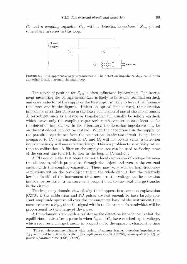
8.2.3 The external circuit and detection 99
Cx and a coupling capacitor Ck, with a detection impedance† Zdet placedsomewhere in series in this loop.
Cx Ck
Zdet
supplyfiltered
measure
Figure 8.2: PD apparent-charge measurement. The detection impedance Zdet could be inany other location around the main loop.
The choice of position for Zdet is often influenced by earthing. The instru-ment measuring the voltage across Zdet is likely to have one terminal earthed,and one conductor of the supply or the test-object is likely to be earthed (assumethe lower one in the figure). Unless an optical link is used, the detectionimpedance must therefore be in the lower connection of one of the capacitances.A test-object such as a stator or transformer will usually be solidly earthed,which leaves only the coupling capacitor’s earth connection as a location forthe detection impedance. In the laboratory, the detection impedance may beon the test-object connection instead. When the capacitance in the supply, orthe parasitic capacitance from the connections in the test circuit, is significantcompared to Ck, the currents in Ck and Cx will not be the same; a detectionimpedance in Ck will measure less charge. This is a problem to sensitivity ratherthan to calibration. A filter on the supply source can be used to forcing moreof the current due to a PD to flow in the loop of Ck and Cx.
A PD event in the test object causes a local depression of voltage betweenthe electrodes, which propagates through the object and even in the externalcircuit with the coupling capacitor. There may very well be high-frequencyoscillations within the test object and in the whole circuit, but the relativelylow bandwidth of the instrument that measures the voltage on the detectionimpedance results in a measurement proportional to the total charge-transferin the circuit.
The frequency-domain view of why this happens is a common explanation[C270]: if the calibration and PD pulses are fast enough to have largely con-stant amplitude spectra all over the measurement band of the instrument thatmeasures across Zdet, then the signal within the instrument’s bandwidth will beproportional to the charge of the pulse.
A time-domain view, with a resistor as the detection impedance, is that theequilibrium state after a pulse is when Cx and Ck have reached equal voltage,which requires a charge transfer in proportion to the apparent charge: the time
† This simple component has a wide variety of names: besides detection impedance orZdet as is used here, it is also called the coupling-device (CD) [C270], quadrupole [Gut95], orpower-separation filter (PSF) [Ste91].

100 Chapter 8: Partial Discharge measurement
integral of the voltage on the resistor over the whole time taken for the circuitto reach a equilibrium is proportional to this charge, so measurement of thisvoltage with the low-pass filter of the instrument’s input gives a response thatis proportional to the apparent charge.
The inductor in Zdet is necessary, at least with ac applied voltage, to let thenormal load-current pass through without much voltage drop. An inductor canalso be used to make the detection have a tuned, narrowband response, ratherthan the wideband response that has a significant bandwidth compared to thecentre-frequency. A capacitor in Zdet can be used to control the peak voltagereached on the detection impedance for a given PD size, and the time-constantwith which the voltage on the detection impedance falls afterwards.
An example of the voltage across a detection impedance and the signal outof the first stage of a PD pulse measurement instrument is shown in figure 8.3.The circuit (see figure 8.2) is a small 2 nF high-voltage ceramic capacitor for
−2000 −1000 0 1000 2000 3000 4000 5000 6000 7000 8000−1
−0.5
0
0.5
1
1.5
time [ns]
v(t)
[V]
−1100 −1000 −900 −800 −7000
0.05
0.1
pre−amp output
pre−amp input(Zdet)
Figure 8.3: Signals at the input and output of the ICM PD instrument’s preamplifier.
each of Cx and Ck, connected by leads on a table. The detection impedanceis a 270Ω resistor; the voltage across it is applied to the ICM instrument’spreamplifier input [s.10.1.1], and also measured by an oscilloscope probe. Thestimulus is a 100pC pulse from the ICM’s calibrator [s.10.1.7], applied acrossCx, and the preamplifier gain is 10. The specification of the preamplifier is afilter-band of 20 kHz to 1.0MHz. The result is that although the current in thecircuit has an oscillatory component, the output from the preamplifier is slowand smooth, with a peak supposedly proportional to the time-integral of theinput. Note how the output too has a damped oscillation: this is its naturalresponse even to a non-oscillatory input, and is significant in PD measurementsif the second peak of the response is measured as a subsequent PD.
8.2.4 Display of results
The phase-resolved PD pattern, PR-PDP or just PDP, is a natural and widely-used way to show results of PD pulse measurements under periodic excitation.Examples can be seen in [s.17.2]. Each detected pulse results in a count beingincremented for the combination of the pulse’s magnitude and the phase of

8.3 Non-pulse measurement of apparent-charge 101
the voltage at which it occurred. The counts form a third dimension on thedisplay, often shown as colour. Using phase rather than time does lose someinformation about variation in the activity, but for many cases it provides auseful simplification. The combination of results from many cycles gives morerepeatable results in spite of the usual variation of PD results between cycles.
Some of the detail in a PDP is potentially interesting to study, but not easilyseen: an example is the total number of PD pulses at a particular phase or ofa particular magnitude. For comparison of multiple PDPs, for example frommeasurements at different voltage amplitudes or on different occasions, it maybe useful to reduce the PDP’s dimension, in order to plot some feature of allof the PDPs together, as will clearly be useful for measurements with variablefrequency [s.15.3.1]. Many forms of reduction are used: the statistical momentssuch as skew and kurtosis are described in [Edi01, p.37], and more physicalvalues such as maximum regularly occurring magnitude, or mean pulse size orcounts per cycle are used.
8.3 Non-pulse measurement of apparent-charge
The C-tan δ measurement [s.6.4.1] sees the fundamental-frequency component ofthe current due to the apparent charges of all the PD. Such ‘bridge methods’ ofmeasuring PD lose all the detail of individual pulses, and have a lower sensitivitybearing in mind the but they have the advantage of coping with high repetitionrates [Bar90] since they do not try to distinguish separate pulses. Methods forshowing the total dissipated energy have been available for decades, such as a‘loop-trace’ method showing dissipated energy as the area within an oscilloscopetrace. It is considered by [Bar90] to be “somewhat astounding that [thesemethods do] not command a higher degree of attention and popularity”. Somereasons may be the perceived importance of the strongest individual sourcesof PD, even if too localised to affect the total current much, and the effect ofdisturbances such as the nonlinear end-winding stress grading.
The DS measurements considered in this work can include some detail of thePD waveform based on the harmonic currents, as shown with artificial pulses inchapter 14 and with real PD in chapter 17.
8.4 Difficulties of PD measurement in stator windings
There are several reasons why the apparent charges cannot be accurately mea-sured as pulses for all the separate PD events in a stator winding. The result isthat, in general, only a small proportion of the total PD charge will be measured.This is not necessarily a bad thing, as measuring just a small sample of the totalpulses may give plenty of information about PD sources, but it does make thenon-pulse methods [s.8.3] interesting as a complement to pulse methods.
8.4.1 Repetition rate
The rate at which PD pulses occur is the repetition rate: when this is high,an instrument working in the low frequency-range of typical apparent-chargemeasurements will not be able to distinguish all the pulses.
Each PD pulse in the system of a winding and external test circuit takes sometime for its oscillations to fade. The conventional apparent-charge measurement
102 Chapter 8: Partial Discharge measurement
has a low bandwidth, to allow the total charge to be measured, but this has thedisadvantage of giving a slow response. The output after filtering is generally os-cillatory: to prevent the pulse measurement system measuring a second peak ofa decaying oscillation as being a second PD of opposite sign, it may be necessaryto have a dead-time during which no further measurement is taken. Deadtimesof tens of microseconds are common in apparent-charge measurements on statorwindings. Insufficient deadtime will result in oscillations of the measurementsystem’s response being recorded as PD pulses. Excessive deadtime will resultin subsequent PD events being missed.
Stator insulation can have such high repetition rates of PD pulses, fromthe many sources throughout a long winding, that many According to [Gro02],thermally aged epoxy-mica insulation can have a repetition rate of 20 000 to100 000 per second. The rather vague range given by [E1434, c.5.1] is that in atypical coil or bar or winding there may be many hundreds of PDs per second;as a winding might consist of a hundred bars, hundreds per bar per second couldalso be taken to indicate a high rate for the complete winding.
8.4.2 Noise and dynamic range
The noise-floor, is the level of background electromagnetic noise that affects themeasurement. In a practical situation this is probably determined by externaldisturbances: in field-measurments of whole machines there are often manysources from other apparatus operating nearby. The measurement instrumenttherefore has to have a discrimination threshold, setting a magnitude belowwhich pulses are ignored. This prevents detection of small pulses that might bepresent.
Additionally, a limited dynamic range of the instrument will result eitherin small pulses being missing or in large pulses causing saturation, dependingon the gain: either of these situations prevents full measurement of the charge.The instrument used in this work has just 128 evenly spaced channels [s.10.1.3]on the linear bipolar range [s.13.5] that is normally used; this is low comparedto the range of pulse-magnitudes that can occur between different PD sourcesin stator insulation [s.7.5].
8.4.3 PD-pulse propagation
Stator windings are certainly in the class of complicated inductive contructions,with consequent troubles of calibration [s.8.2.2]. The relevant standards forPD measurement, such as [E1434] and [C3427], warn against use of ‘apparentcharge’ terminology, pointing out that the results cannot be compared to thosefrom other objects or measurement systems.
On the other hand, laboratory work with stator insulation usually involvesjust a single bar or coil, with all the high-voltage conductors joined. Thisis true for the laboratory measurements in this work, and for industrial testsof new insulation systems. In this case, valid calibration of apparent-chargemeasurements can be made [C3427, c.10.2.1]. The problem of large numbers ofsources is reduced when dealing with only one or a few bars, but there may stillbe too high a repetition rate for an apparent-charge PD instrument to be ableto capture each pulse.

8.4.3 PD-pulse propagation 103
There was a period starting around 1990 when several groups researchedPD signal transmission in stator windings, mainly with the aim of achieving anacceptable standard level for PD testing. The method was typically injectionof controlled charges at different points in a winding, and measurement of theresult at the terminals. Some of these pulse-propagation studies are cited in asummary in [E1434].
There is a strong distinction found between a ‘fast’ component of the signal,consisting of high-frequencies that travel to the terminals by shorter routes thanpropagation along the path of the winding, and a ‘slow’ component of lowerfrequencies whose transit time is proportional to the length of winding betweenthe PD site and the measurement. The boundary between the frequencies ofthese fast and slow components is in the region of 1MHz, but is defined or seendifferently by different groups, and in some cases only the slow component isobserved.
The fast coupling is of little interest for apparent-charge measurement be-cause the resonances and attenuations in this range make the result very de-pendent on where the PD occurred. The fast mode is highly attenuated withinthe windings, by reflections at the transitions of the ∼20Ω to 30Ω slot partsand the ∼300Ω end-windings [E1434], and transmission-line attenuation dueto the the semiconducting layers at high frequency [Gro02]. The nature of thefast coupling that permits a shorter route than following the winding is notunanimously agreed: it is shown experimentally in [Pem06] that the absenceof end-windings prevents the fast coupling, but in [Tav88] inductive couplingbetween slots is expected for frequencies even up to 20MHz, for large machines;in [Gea90] the fast coupling is thought to be capacitive, but in [Zhu92] it iswondered whether it is in fact more inductive.
The slow, low-frequency, ‘travelling wave’ mode propagates along the con-ductors of the winding, possibly with inductive coupling to other bars. Theattenuation of this slow mode is very low, and its propagation speed is givenfrom about 10m/µs [Pem06] to over 100m/µs [Zhu92] by different references.
The frequency range of a few tens to a few hundreds of kilohertz gives thelowest variation in measured apparent charge. According to [Sto98] this rangemay still not be very flat, but others show quite a flat response, such as [Woo93]with spectrum-analyser (not apparent-charge) results, and [Pem06] with verylittle location-dependence in charge but a few times variation in voltage peaks.
The recommendation of [C3427, c.5.2] is to use wideband measurementsin accordance with IEC-60270, with lower cutoff of tens of kilohertz. This ischosen in order to have ‘sufficient visibility’ of sources that are deep in thewinding, but it is warned that there may be resonances even in this range. Therecommendation of [E1434] is that offline tests on complete windings shouldmeasure at frequencies below 500 kHz, but that this has the disadvantage ofpulse superposition of pulses when the repetition rate is near the instrumentbandwidth.

104 Chapter 8: Partial Discharge measurement
8.5 Current practice in stator-PD measurement
There are many types of PD measurement made on rotating machines. A goodsummary of electrical methods is [E1434]. Rotating machines are unusual amonghigh-voltage apparatus in not having specifications of acceptable PD levels. Thisis due to the trouble of calibration [s.8.4], the large magnitudes that can betolerated by the mica-based insulation, and the great difference in acceptablemagnitude between different types of PD source [s.7.5].
Online PD measurements are common on large or important machines,giving good trending and warning of rapid changes in activity. Some of thesesystems are very different from apparent-charge measurements, using a highfrequency range of the order of tens of megahertz, with multiple detectionlocations and comparison of time of arrival.
Offline measurements are common as part of asset management of rotatingmachines. It is usual to measure at several amplitudes of an applied sinusoidalvoltage at power frequency. The offline measurements can take advantage ofexciting different combinations of windings, to distinguish different PD sites suchas ones from phase to earth or from phase to phase [C3427]. The attenuationof PD pulses in the winding makes it sometimes worthwhile to measure at thephase and neutral ends of a winding separately, as a primitive step towardslocation of sources. The lower frequency apparent-charge style measurementis common, often using PDPs to analyse the results. Derived quantities arepopular too, such as distributions of pulses by phase or magnitude, largestrepeatedly occurring PD magnitude, quadratic rate (using the square of themagnitude), and simple calculations of energy based on the supply voltage atwhich a pulse occurred.

Chapter 9
The Dielectric Spectroscopy instrument
This chapter describes the operation and specification of the DS instrumentused in this work, and the new programs that were written to control it. Muchof the information here is not documented with the instrument, so is hopedto be a useful summary for future users in our laboratory and possibly forusers elsewhere. The details are relevant to the combined use of the DS andPD instruments and to discussion in chapter 14 of measurement of PD pulses.Some tests of the instrument are described in chapter 12.
9.1 Description of the IDAX300 and HVU
A commercially available DS measurement instrument was chosen for applyingand measuring the test voltage and for measuring the current through theinsulation system. This is the IDAX 300 from Pax (now Megger) of Taby,Sweden, shown in figure 9.1. Earlier instruments from this model-family arewell known in our group: the IDA 200 was used in the work of [Tay06], andthe earlier instruments were developed in the course of the work described in[Wer01a].
Figure 9.1: The IDAX 300 DS-instrument (left) and its HVU (right).
The choice was motivated by the convenience of having a compact andtested construction of the sensitive measurement components along with theirprotection and shielding, with the calibration already done. Discussion withthe manufacturer suggested that the sufficient information could be providedfor the writing of control-programs other than the supplied one.
The IDAX’s main unit contains all the components needed to supply si-nusoidal voltages at amplitudes up to 200V and frequencies from 100µHz to10kHz, and to measure this voltage and the current through the test object,performing DFTs to present the measured data in frequency-domain form.
A high-voltage output can be provided by an external amplifier supplied asan accessory to the IDAX, referred to as the high-voltage unit, HVU. Use of theHVU limits the maximum frequency to about 100Hz. The HVU used in this
105
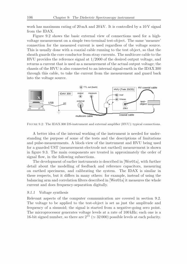
106 Chapter 9: The Dielectric Spectroscopy instrument
work has maximum rating of 20mA and 20 kV. It is controlled by a 10V signalfrom the IDAX.
Figure 9.2 shows the basic external view of connections used for a high-voltage measurement on a simple two-terminal test-object. The same ‘measure’connection for the measured current is used regardless of the voltage source.This is usually done with a coaxial cable running to the test object, so that thesheath guards the core conductor from stray currents. The multicore cable to theHVU provides the reference signal at 1/2000 of the desired output voltage, andreturns a current that is used as a measurement of the actual output voltage; thechassis of the HVU is also connected to an internal signal-earth in the IDAX300through this cable, to take the current from the measurement and guard backinto the voltage source.
IDAX 300 measure
coaxial cable
HVU (Trek 20/20)
20kV
multicore cable
USB
Vrefoutput
externalVmeas
TTL out (back)
objecttest−
HV coaxial cable
Figure 9.2: The IDAX300 DS-instrument and external amplifier (HVU): typical connections.
A better idea of the internal working of the instrument is needed for under-standing the purpose of some of the tests and the descriptions of limitationsand pulse-measurements. A block-view of the instrument and HVU being usedfor a guarded UST (measurement-electrode not earthed) measurement is shownin figure 9.3. The main components are treated in approximately the order ofsignal flow, in the following subsections.
The development of earlier instruments is described in [Wer01a], with furtherdetail about the modelling of feedback and reference capacitors, measuringon earthed specimens, and calibrating the system. The IDAX is similar inthese respects, but it differs in many others: for example, instead of using thebalancing arm and correlation filters described in [Wer01a] it measures the wholecurrent and does frequency-separation digitally.
9.1.1 Voltage synthesis
Relevant aspects of the computer communication are covered in section 9.2.The voltage to be applied to the test-object is set as just the amplitude andfrequency of a sinusoid; the signal is started from a negative-going zero point.The microprocessor generates voltage levels at a rate of 100 kHz; each one is a16-bit signed number, so there are 215 (≃ 32 000) possible levels at each polarity.
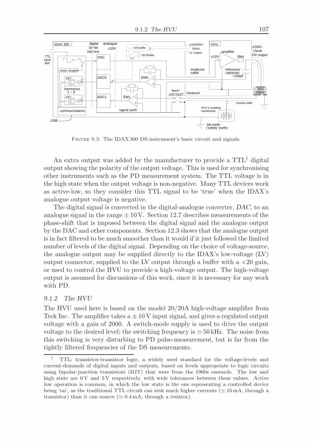
9.1.2 The HVU 107
+−EM1
+−EM0
IDAX 300 HVU
±10V
measure
signal earth
ADC0
DAC
ADC1
TTLsyncout
filter
communications
USB
harmonics1 − 8 object
test
digital
100 kHz16−bit
analogue±10V ×20 buffer
÷20 divider
clock, sinegen
HV output15mA±20kV
±(10|200)V50mA
LV output
multicorecable
HVU’s isolatingtransformer
coaxial cable
lab earth(‘safety’ earth)
‘reference’capacitor
~100pF
amplifier
UST/GST‘term’
DFT
DFT
Figure 9.3: The IDAX300 DS-instrument’s basic circuit and signals.
An extra output was added by the manufacturer to provide a TTL† digitaloutput showing the polarity of the output voltage. This is used for synchronisingother instruments such as the PD measurement system. The TTL voltage is inthe high state when the output voltage is non-negative. Many TTL devices workas active-low, so they consider this TTL signal to be ‘true’ when the IDAX’sanalogue output voltage is negative.
The digital signal is converted in the digital-analogue converter, DAC, to ananalogue signal in the range ± 10V. Section 12.7 describes measurements of thephase-shift that is imposed between the digital signal and the analogue outputby the DAC and other components. Section 12.3 shows that the analogue outputis in fact filtered to be much smoother than it would if it just followed the limitednumber of levels of the digital signal. Depending on the choice of voltage-source,the analogue output may be supplied directly to the IDAX’s low-voltage (LV)output connector, supplied to the LV output through a buffer with a ×20 gain,or used to control the HVU to provide a high-voltage output. The high-voltageoutput is assumed for discussions of this work, since it is necessary for any workwith PD.
9.1.2 The HVU
The HVU used here is based on the model 20/20A high-voltage amplifier fromTrek Inc. The amplifier takes a ± 10V input signal, and gives a regulated outputvoltage with a gain of 2000. A switch-mode supply is used to drive the outputvoltage to the desired level; the switching frequency is ≃ 50kHz. The noise fromthis switching is very disturbing to PD pulse-measurement, but is far from thetightly filtered frequencies of the DS measurements.
† TTL: transistor-transistor logic, a widely used standard for the voltage-levels andcurrent-demands of digital inputs and outputs, based on levels appropriate to logic circuitsusing bipolar-junction transistors (BJT) that were from the 1960s onwards. The low andhigh state are 0V and 5V respectively, with wide tolerances between these values. Activelow operation is common, in which the low state is the one representing a controlled devicebeing ‘on’, as the traditional TTL circuit can sink much higher currents (≃ 16mA, through atransistor) than it can source (≃ 0.4mA, through a resistor).

108 Chapter 9: The Dielectric Spectroscopy instrument
The amplifier’s maximum output current is limited by the amplifier’s internalregulation, with an absolute maximum of 20mA and lower limits for partsof the current/voltage operating curve where the voltage is low or the powerflow is into the amplifier. A distorted output voltage waveform will result ifthe combination of requested amplitude and frequency would cause more thanthe amplifier’s current-limit in the connected load. The current drawn fromthe voltage source consists of the current through the test-object, measuredin the current-electrometer EM1, the current through the reference capacitor,measured in voltage-electrometer EM0, and all currents that are guarded awayfrom the electrometers, the shielded high-voltage cable giving a substantialcontribution to this.
The reference capacitor in this HVU is a short length of cable with XLPE(cross-linked polyethylene) dielectric; its properties are included in the calibra-tion data by specifying the complex capacitance over a range of frequencies.
9.1.3 Voltage measurement
DS requires very high accuracy for the measurement of relative phase betweenvoltage and current. The applied voltage is therefore measured at the outputterminal rather than being inferred from the signal just before or after the DAC.The analogue-digital converter ADC0 accepts a ± 10V signal: the low-voltage10V output can thus be measured directly. The low-voltage 200V output ismeasured through a 1/20 resistive divider, and the high-voltage output in newIDAX units is also measured as a voltage signal from a divider.
In the system used here, however, for compatibility with the old HVU andthe earlier IDA200 instrument, an older method is used, measuring the currentthrough a known HV ‘reference’ capacitor. Converting this current to a voltagesignal into ADC0 requires a further electrometer ‘EM0’ besides the one usedfor measuring the current through the test-object. The two electrometers aresimilar in specification; the description in section 9.1.5 provides the details.
9.1.4 Specimen earthing
In figure 9.3 the test-object electrode whose current is to be measured is floatingwith respect to earth; it can be connected directly to the input of the elec-trometer EM1. The signal earth of the circuit of the electrometer and voltage-source can therefore be connected to the instrument’s chassis and thereby to thesafety earth that connects to the chassis of all the instruments and the buildingstructure and the earth itself; any electrodes whose current is to be guarded canalso be connected to earth. The relays marked ‘term UST/GST’ in figure 9.3are shown in this configuration, which is referred to as ‘unearthed specimentest’, UST. Stray currents between the supply voltage and any conductor otherthan the measurement electrode are guarded away from the measurement; thisdesirable situation is usually able to be achieved in a laboratory measurement.
In a measurement on installed apparatus such as stator windings or cables,there is often a measurement electrode that cannot feasibly be disconnected fromsafety earth: the stator iron is typically in electrical contact with the buildingconstruction, and a cable’s sheath is often bonded to switchgear or in significantcontact with soil. If the signal earth in the instrument were also connected to

9.1.5 Electrometers and feedback 109
safety earth as in the UST configuration, the current to be measured couldbypass the electrometer by returning to the voltage source by passing throughthe test-object and instrument earth connections. The ‘grounded’ (earthed)specimen test, GST, swaps the connections so that the electrometer input isconnected to safety earth and the ‘measure’ input provides a bypass straight tosignal earth for any guarded electrodes. For this to work, the voltage sourcemust draw its current from the signal earth, and not connect signal earth tosafety earth. The HVU draws its current from its chassis: in order to permitGST measurements with high voltage, the HVU has to be supplied throughan isolating transformer with shielding to minimise capacitively coupled humcurrents [Wer01a, p.68]. A disadvantage is that any stray currents to earthedelectrodes will be measured by the electrometer.
The matter of earthed or floating measurement electrodes becomes impor-tant when considering how to combine the IDAX with the ICM PD pulse-measurement instrument for simultaneous measurements in the laboratory andin the field. Practically any field-measurement on a stator winding must acceptthe stator as being solidly and unavoidably earthed.
9.1.5 Electrometers and feedback
A description of the purpose and practical details of feedback electrometers forDS measurement is given in section 6.2. The details known about the IDAXelectrometers are the parameters from the instrument’s calibration data. Theopen-loop gain is modelled as low-frequency value of 6.3×10⁵ with frequency-response of single-pole filter with pole-frequency about 30Hz. Its input ca-pacitance is 12 pF. The output voltage is restricted to ± 9V, with feedbackcomponents chosen to yield a considerably lower value, such as 7 V or less, withthe expected test-object. The output voltage is measured in an analogue-digitalconverter and is used to calculate the input current according to (6.8).
One resistive and one capacitive feedback component can be selected byrelays, to connect in parallel between the output and input of the electrometer.The available resistances are 10(1+nr) Ω where the integer nr is in the range1 ≤ nr ≤ 9 giving a range of 100Ω to 10GΩ; the special value nr = 0 gives anopen circuit, specified as a finite value of 1018 Ω. The available capacitances are10−(4+nc) F, with 1 ≤ nr ≤ 6, a range of 10µF down to 100pF. These intendedvalues are listed in table 9.1, along with examples of the reactances of thecapacitors at different frequencies. For adequate calculation of the current intothe electrometer the feedback values must be known very precisely, includingany significant frequency-dependence. Actual measured values of the feedbackcomponents are stored in the calibration data [s.9.1.7] and are used for thiscalculation. For choosing which feedback components to use, the nominal valueslisted in table 9.1 are sufficient.
The complex capacitance C is calculated as the ratio of the measured com-plex current I and voltage V . For a measurement using the HVU, these quanti-ties are in turn calculated from measured voltages at the outputs of electrometersEM1 and EM0, Vo1 andVo0, based on electrometer and feedback properties(6.8). Ignoring the effect of the term multipled by H(ω) in (6.8), as thoughthe electrometer calibration and extra shunt impedance are correctly known,
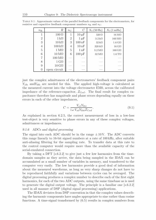
110 Chapter 9: The Dielectric Spectroscopy instrument
Table 9.1: Approximate values of the parallel feedback components for the electrometers, forresistive and capacitive feedback component numbers nR and nC.
nR R nC C XC(50 Hz) XC(1mHz)
1 100Ω 1 10µF 320Ω 16MΩ
2 1 kΩ 2 1µF 3.2 kΩ 160 MΩ
3 10 kΩ 3 100nF 32 kΩ 1.6GΩ
4 100kΩ 4 10 nF 320 kΩ 16GΩ
5 1 MΩ 5 1nF 3.2MΩ 160GΩ
6 10MΩ 6 100pF 32 MΩ 1.6TΩ
7 100MΩ — — — —8 1 GΩ — — — —9 10GΩ — — — —0 open circuit — — — —
just the complex admittances of the electrometers’ feedback component pairsY1fb andY0fb are needed for this. The applied high-voltage is calculated asthe measured current into the voltage electrometer EM0, across the calibratedimpedance of the reference-capacitor, ZCref . The final result for complex ca-pacitance therefore has magnitude and phase errors depending equally on theseerrors in each of the other impedances,
C =Vo1Yfb1
i ω Vo0Yfb0ZCref. (9.1)
As explained in section 6.2.5, the correct measurement of loss in a low-losstest-object is very sensitive to phase errors in any of these complex voltages,admittances or impedances.
9.1.6 ADCs and digital processing
The signal into each ADC should be in the range ± 10V. The ADC convertsthis range linearly to 16-bit signed numbers at a rate of 100 kHz, after suitableanti-aliasing filtering for the sampling rate. To transfer data at this rate tothe control computer would require more than the available capacity of theserial-emulated connection.
By taking a DFT [s.6.2.2] to give just a few low harmonics from the time-domain samples as they arrive, the data being sampled in the IDAX can beaccumulated as a small number of variables in memory, and transferred to thecomputer very easily. The low harmonics provide a good deal of informationabout the measured waveforms, as long as very sharp changes do not have tobe reproduced faithfully and variations between cycles can be averaged. Thedigital processing produces a complex number to describe each of the first eightharmonics, for each of the two ADC outputs, using the same timebase as is usedto generate the digital output voltage. The principle is a familiar one [s.6.2.2]used in all manner of DSP (digital signal processing) applications.
The IDAX deviates from DSP convention in that the complex values describ-ing the harmonic components have angles appropriate to sine rather than cosinefunctions. A time-signal transformed by (6.5) results in complex numbers from

9.1.7 Calibration 111
which the time-signal, or a filtered version using just limited harmonics, canbe recovered by summing cosines as in (6.7). The complex values Sn from theIDAX should be used in sine functions to approximate the measured waveform,
s(t) =N∑
n=0
|Sn| sin (nωt + ∠Sn) . (9.2)
For any single harmonic order this distinction between sine and cosine is merelya time-shift, which is irrelevant when zero time has no special meaning. For non-sinusoidal waveforms, where multiple harmonic orders are added, it is essentialto use the right function in order to preserve the shape of the waveform: theequal phase-shifts of the harmonics between the sine and cosine forms corre-spond to different time-shifts. Conversion of Sn between the sine or cosine formrequires a phase-shift of n∠Sn.
The absolute phase of the complex numbers returned by the IDAX’s DFTappears to be based on the internally generated digital signal, while for the olderIDA200 instrument it appeared quite arbitrary. The important matter is therelative value of phase between the measured voltage and current signals fromthe ADCs, each phase measured relative to the common reference. A dc term,h = 0, is also available from the DFT, this being the mean value of the samples.When capacitive feedback is used, the dc term is not directly convertible tovoltage or current at the test-object. In the normal use of the IDAX the dcterm is only used for checking on dc input currents when selecting suitablefeedback. If using resistive feedback the information in this dc term would begood to have when measuring on asymmetric test-objects that have a non-zeromean.
In the IDAX’s processing, the samples and their coefficients are signed 16-bit integers. To limit the rate at which new results must be checked for andtransferred, the IDAX accumulates DFT results over whichever is the greatertime of 1 s or the smallest integer number of cycles that takes more than 1 s.After this, the result is available for transfer as a list of integers in text form,and a fresh accumulation is made. For very low frequencies with periods ofthousands of seconds, the accumulation of 100kHz sampling of 16-bit integersmultiplied by 16-bit integer coefficients leads to very large numbers, such thatone must be careful to use suitable storage and manipulation on the controlcomputer; double-precision floating point numbers were used throughout thecontrol program, to ensure sufficient representation.
9.1.7 Calibration
The DFT components calculated from the two ADC outputs have to be con-verted into the applied voltage and the resulting current at the test-object. Thiscalculation requires knowledge of transfer functions of many of the instrument’scomponents. Stored in the instrument is a calibration file that can be copiedto the control computer when the instrument is connected. This file includesdetails of components’ limits and transfer-functions. Some components, forexample feedback resistors, are modelled as constants; others, for examplethe reference capacitor and feedback capacitors, are modelled as ‘universal

112 Chapter 9: The Dielectric Spectroscopy instrument
capacitors’ following multiparameter equations as described in [Wer01a]; others,for example the buffer and divider used for the 200V output, or the relativeamplitude and phase between the two ADCs, are modelled as measurementsat several frequencies, with linear interpolation. The values already in thecalibration file when the instrument was delivered from the manufacturer havebeen used in all this work.
The instrument’s specification gives an operating temperature range of 0 Cto 55 C, and timebase relative accuracy of 10−4. The accuracy of capacitancemeasurements is expressed as the maximum error for the case of the inter-nal 200V voltage source with ‘optimal’ choice of feedback components anda stipulated maximum hum-current. For capacitance C′ the claimed error is0.5%+1pF. For tan δ across the range of frequency and measured capacitance.1%+3×10⁻⁴ and 2%+2×10⁻³
Accuracy of absolute values is certainly desirable for permitting comparisonsof measurements made with different instruments; the consistency of relativevalues, however, is much more important in this work where one instrument willbe used and where there is interest in the very small changes in the measuredcapacitance and loss due to PD activity.
9.2 Computer control
The IDAX 300 is connected to the control computer by USB, using serial-emulation to appear as a serial-port device. Purely text-based communication isused to send commands, retrieve the measurement data, and transfer calibrationdata back and forth. The program that is provided with the IDAX for runningon the control computer was unsuitable for this work: it runs only on a typeof operating system that we have learnt to avoid, it has no means of beingcombined with other programs to coordinate DS and PD measurements in aloop, and it automates more of the settings such as feedback than seems desirablefor this work. A control program was written using the Instrument ControlToolbox of the proprietary numerical-computing program ‘Matlab’ to providethe functions for serial communication. This could easily have been achievedin for example GNU Octave, but it was considered important that future userswould be working in an environment already familiar to them.
There are of the order of a hundred commands that can be sent to theinstrument for setting the voltage amplitude and frequency, setting feedbackcomponents and the ‘termination’ settings for UST or GST measurements,transferring calibration data, checking on a running measurement, and retriev-ing results. These commands, like all the details of the IDAX instrument otherthan the use of its supplied GUI control program, were undocumented. Some‘reverse engineering’ was needed in order to deduce suitable commands to setup the output voltage, relay settings and feedback, and the request the resultsand convert them into physical values at the test-object. This was done bystudying logs of the communications between the IDAX and its supplied GUIprogram, and by obtaining and reading some of the program-code used in thosecomponents, followed by a good deal of testing. Many sets of commands, suchas those sent during initialisation or for setting the voltage sources, have simply

9.3 Automatic selection of feedback-component values 113
been accepted as blocks of ‘recipe-book’ programming, with no convenient wayof determining what the individual commands do.
Functions have been written to do all the main tasks of connecting, calcu-lating suitable feedback, setting up, starting a measurement, getting the resultsand converting them to physical parameters. To make a measurement, a scriptis run that calls the appropriate functions; for simple measurements only a veryfew lines of code are needed in this script. Many variations have been used forrunning tests and measurements with the IDAX on different types of test-objectand in combination with other instruments such as the PD-pulse measurementinstrument or function-generators and oscilloscopes. All raw results as well asderived results and time information are stored in a variable that is saved atthe end of a sweep. The text displayed on screen during the sweep is loggedcontinuously, and a copy of the script is saved before each sweep. This level ofdetail has several times been useful when investigating apparent problems withdata.
9.3 Automatic selection of feedback-component values
The choice of suitable feedback components for an electrometer has been par-tially covered in section 6.2.6. Many factors must be considered. The feedbackcurrent should be always mainly in the resistor or mainly in the capacitor. Avery low-capacitance object at low frequency may have such high impedancethat even the highest-value available feedback resistance (apart from the opencircuit option) would give unacceptably low electrometer output voltage; ca-pacitive feedback is needed in this case. A very high-capacitance object mayhave such low impedance that even the largest feedback capacitor would requireelectrometer output voltages higher than the electrometer’s range; resistivefeedback is needed in this case. An object with considerable conductance mayrequire resistive feedback in the low-frequency range where the long times allowlarge charges to flow. To make sure that the electrometer output voltage willnot hit its limits, the feedback components must be chosen based on severalmatters other than the test-object and the applied signal. Electric or magneticfields, and extraneous currents sharing part of the measurement circuit, mayintroduce hum currents in the measurement circuit, typically at the electricity-supply frequency. There may be a dc component in the input current or fromthe electrometer output, which would cause a ramping voltage with capacitivefeedback or a constant extra voltage with resistive feedback. Any slow-decayingoffset in the electrometer output, due to the use of nearly pure capacitivefeedback together with a significantly conductive test-object, would shift theelectrometer voltage closer to one of its limits.
The GUI program supplied with the IDAX does a lot of work measuringinterference from hum and dc, assessing the test-object, using rules to determinefeedback components, and revising the choice if any overload is detected; thismakes the instrument suitable for automatic measurements on a range of HVcomponents.
In this work and for later users of the IDAX in the lab it was thoughtbetter to involve the user more in the decision. Each measurement is made
114 Chapter 9: The Dielectric Spectroscopy instrument
from a program script [s.A.3.3], which makes it possible for the user to specifyarbitrary rules for feedback based on knowledge of the test object and its possiblenonlinear or pulsed behaviour. It might for example be that changes betweencapacitive and resistive feedback should be avoided, or that any big changes inCFBR should happen at the same frequency within each of several sweeps atdifferent voltage amplitudes.
For awkward test-objects such as samples of highly nonlinear resistive ma-terial, the feedback was set in the script, using a material model to predict thecurrent, then using the feedback resistor of resistance one decade lower thanwas calculated, to give a wide safety margin. For simpler objects, a functionwas written to automate choice of feedback components based on frequency, theexpected complex-capacitance of the test-object, a preferred CFBR, and themaximum desired electrometer output voltage. The dominant type of feedbackcomponent was chosen to ensure the maximum electrometer voltage would notbe exceeed. The other component was then set to whatever came closest to therequested CFBR. Practically all the measurements have actually been madewith strongly resistive CFBR, around 1% or less.
Some simplifying features in most of this work are that: the problems ofhum and dc currents are less in laboratory than in industrial environments; theresolution of the IDAX’s ADCs makes it usually quite acceptable to fall even to1/100 of the maximum possible electrometer output voltage, so a large marginof safety can be left to avoid electrometer overloads in difficult cases involvinginterference, pulses, or nonlinear test-objects.
9.4 Alternative types of instrument
Data-acquisition (DAQ) hardware can provide multiple digital and analogueinterfaces between a computer and other equipment. The sample-rates andprecisions now available would easily match those of the IDAX’s DAC andADCs at a much lower price than a specialised instrument, and would allowfull time-domain waveforms to be recorded and arbitrary voltage signals tobe generated. This, however, is only a part of the instrument’s function. Atleast one electrometer is essential for measuring the tiny currents of subpicoamplevels, even if the output voltage can be measured directly from a divider.Electrometers of this specification are not cheap, and they require a set of well-defined feedback components with computer-controlled switching. The sensitivecomponents must be protected against the high currents and overvoltages thatcan result from for example a short-circuit in the test-object, but the protectivedevices must avoid disturbing the tiny current of normal measurements; someof the earlier work on protection is described in [Wer01a, p.41]. Calibrationis needed for the amplitude and phase responses of several of the componentsin the signal path, as well as of feedback-component values. Having all thesefeatures already combined and tested in a compact instrument is thus worth a lotmore than just the analogue/digital interface properties. It would neverthelessbe worthwhile to consider the alternatives carefully in any future measurementsystem, particularly if wanting more versatile control of the output signal or ofthe detail of recorded results.

Chapter 10
The PD pulse-measurement instrument
This chapter describes the operation and specification of the PD instrumentused in this work, and the programs that were written to control it. As withthe DS instrument in chapter 9, these details are of relevance when consideringhow to combine the DS and PD instruments and when analysing results. Moreof the detail of the PD instrument is already documented, so this chapter ismainly a summary. Some tests of the instrument are described in chapter 13,to determine undocumented details and assess the reliability of results.
10.1 Description of the ICM components
A commercially available instrument designed for use according to IEC-60270has been used for the PD pulse-measurements reported in this work. This isthe ICM-system, from Power Diagnostix Systems GmbH of Aachen, Germany,shown in figure 10.1 together with its preamplifier. A diagram of the basicconnections is shown in figure 10.2, using the same physical layout. The choice
Figure 10.1: The ICM PD-pulse measurement instrument: the main unit is in thebackground, with its input connected to a preamplifier in the foreground.
was partly due to this type of instrument having been shown in the earlier workof [Edi01] to work for PD measurements at very low frequencies. An ICM ofmodel version 7.60 was bought in 2007, supplementing the existing one of modelversion 2.00. The newer version had some differences from the old one, and somedifferences from its manual; various problems had to be worked around.
The ICM’s main unit is a chassis containing modules that provide am-plification, registration of PD pattern, and communication with a controllingcomputer. Some preamplification and buffering functions are done in external
115

116 Chapter 10: The PD pulse-measurement instrument
boxes to allow these functions to be nearer to the signal source. The ICMis connected to the control computer by GPIB (general-purpose interface bus,IEEE-488). The control computer sends text-based commands to control all thesettings, start acquisitions and request results.
DPR3AMP3 CTRL3
in
out in
in
GATE3 ADC3
HST1
gating signal
controller
GPIB
TTL sync input
RPA1Zdet
PD circuit
pre−amplifier
synchroniserand PR−PDPmemory
amplifiermain digitiser
coaxial cable50 Ω sync inputanalogue
Figure 10.2: The ICM PD-instrument’s main components. Gating has not been used in thiswork. The controller module communicates with all the others.
10.1.1 Preamplifier
The signal from a PD source reaches the ICM through a preamplifier. Severalinterchangeable preamplifiers are available to provide extra features such asoptical isolation, ultrasonic transduction, or translation of higher frequency-bands down to the 40 kHz to 800kHz band treated by the ICM.
The RPA1 preamplifier has been used in all the work here. It has the simplefunction of providing the first band-pass filtering and amplification of the PDsignal, buffering the possibly long signal cable from the PD source so that thecable does not affect the effective detection impedance. Its BNC input-connectorhas a loading of 10kΩ and 50 pF. Its BNC output-connector connects to themain-amplifier through a 50Ω coaxial cable whose length can exceed even 40mif low-loss cable is used. The main amplifier provides a dc voltage to powerthe preamplifier and to set its gain to the available multipliers of 1, 10 or 100.The PD signal from the preamplifier is superimposed on the same cable, and isac-coupled into the main amplifier. The 6 dB (impedance) bandwidth is fixedat 20 kHz to 1.0MHz, a little wider than the system’s widest bandwidth, witha roll-off of 40 dB/decade.
10.1.2 Main amplifier
The main-amplifier is the AMP3 module in the ICM. The input BNC connectorhas input impedance of 50Ω to ac signals, and provides a superimposed dcvoltage to power the preamplifier unit and control its gain. Its nominal gainsare all the products of a multiplier (1,2,4,8) and scaling (1,10,100). Its lower−3 dB cut-off frequency f1 can be selected as 40, 80, 100 kHz, and its uppercut-off frequency f2 as 250, 600, 800kHz.
The AMP3 module also contains a peak-meter (sometimes called a ‘charge’or ‘picocoulomb’ meter as the voltage peaks are supposed to relate to apparentcharge). This measures the magnitude, ignoring polarity, of the output signal,quantising the 0V to 5 V range linearly into 12bit resolution. The peak-meter

10.1.3 Digitiser 117
charging time is quoted as 0.5µs, suggesting that the recorded value reflects anaverage over this time. The value returned when the peak-meter is read seemsto update only every half second or so, suggesting that it is the highest value inthe last such period. Constant display of the peak reading is interesting whenwatching an ongoing measurement or when trying to reduce noise sources, butthe only PD results shown for real test-objects in this work have come from thelater ADC3 quantiser module that forms the PD pattern.
The normal output voltage range of the AMP3 should be ± 5 V, to be withinthe limits of the ADC3 conversion module and of the AMP3’s own peak-meter.The actual output voltage can be considerably more: over +10V has beenobserved on an oscilloscope during tests of extreme inputs and settings.
10.1.3 Digitiser
The ADC3 module contains the ADC (analogue-digital converter) that is usedin producing the phase-resolved PD pattern [s.8.2.4]. The signal-flow diagramof figure 10.3 shows the main functions of this module in three stages.
The first part, ‘acquisition logic’, decides when the input signal should besent for quantisation in the following ADC. This is actually rather complex: itis simplified in the diagram partly because the abstraction provides sufficientinformation and partly because we do not have much more detail than this aboutthe inner workings. The LLD (low-level discriminator, or threshold) sets a lowerlimit to the voltage magnitude that must be present to cause any measurementat all; this is used to avoid measuring background noise. The choice of first-peak or time-window, along with a deadtime, determines how multiple peaksshould be treated. With first-peak, a peak exceeding the LLD level will besent for conversion in the ADC, then no further peak will be recorded for thedeadtime, which can be set from 5 µs to 3ms; the purpose of the deadtime isto avoid acquisition of subsequent peaks of the oscillatory voltage that a pulseinput to the amplifier causes on the amplifier’s output. With time-window, thedeadtime defines a period over which the greatest positive and greatest negativepeak are held, and the greater of these values is then converted. In this workthe first-peak setting was used, with a deadtime as small as possible while notseeing signs of acquiring reverse-polarity peaks.
The ADC quantises voltages in a ±5V range into 212 (4096) digital levels,with a 0.5µs conversion time. Only 28 (256) levels are used in the phase-resolvedPD pattern, so the 2048 levels have to be mapped onto 256 charge-levels; severalmappings, referred to as the ADC characteristics, are available for making thebest use of the 256 charge-levels for different applications. The linear bipolarcharacteristic is the most obvious, mapping each group of 16 values of ADCoutput into a single one of the PD pattern charge-channels. For cases wherethe input’s polarity is not important, the linear unipolar characteristic doublesthe magnitude-resolution by neglecting the pulse polarity. Other options involvenonlinear mappings with a logarithmic or sine relation to enhance the resolutiontowards one end of the magnitude scale. In this work linear bipolar has beenused, as we are always dealing with bipolar signals and no great advantage wasseen in the nonlinear mappings.
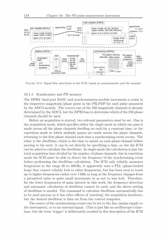
118 Chapter 10: The PD pulse-measurement instrument
256 x t dwell
upper cutoffs: 250, 600, 800 kHzlower cutoffs: 40, 80, 100 kHz
gains of (1,2,4,8)*(1,10,100)
−5V
+5V
ADC
log biplin uni
log uni
lin bip
sinesqrtsine
4096
Ω
~500 ns
digitiser (ADC3)
main amplifier (AMP3)
compress:nonesingle
double
PD patterntransfer
sync/memory (DPR3)
‘characteristic’
levels256
levels
conversion time
50input
TTLexternal
linesync source:
pre−amplifier (RPA1)
lower cutoff: 20 kHzupper cutoff: 1 MHzgains of (1,10,100)
inputΩ2.5 k
−2.5V+2.5 Vsignal limits
10 k Ω50 pF
input
~ 10 V dc level
256x256, 16bit countsPD pattern memory
deadtimefirst/windowLLD
Acquisitionlogic:
100 Ωoutput
charge meter
0 < |V| < 52048 levels
data
(PDP)output
nominal +−5 V>+−10 V
signal limits
Figure 10.3: Signal flow and limits in the ICM, based on measurements and the manual.
10.1.4 Synchroniser and PD memory
The DPR3 ‘dual-port RAM’ and synchronisation module increments a count inthe respective magnitude/phase point in the PR-PDP for each pulse measuredby the ADC3 module. The correct one of the 256 magnitude channels is alreadydetermined by the ADC3, but the DPR3 has to determine which of the 256 phasechannels should be used.
Before an acquisition is started, two relevant parameters must be set. One isthe acquisition mode, which specifies either the single mode in which one pass ismade across all the phase channels dwelling on each for a constant time, or therepetition mode in which multiple passes are made across the phase channels,returning to the first phase channel each time a synchronising event occurs. Theother is the dwelltime, which is the time to spend on each phase-channel beforemoving to the next: it can be set directly by specifying a time, or else the ICMcan be asked to calculate the dwelltime. In single mode the calculation is just thetotal acquisition time divided by the number of phase-channels, but in repetitionmode the ICM must be able to detect the frequency of the synchronising eventbefore performing the dwelltime calculation. The ICM only reliably measuresfrequencies in the range 30 to 400Hz; it apparently uses a PLL (phase-lockedloop) that cannot reliably lock to other frequencies, but has been seen to trackup to higher frequencies rather over 1 kHz as long as the frequency changes froma permitted value in quite small increments so as not to lose lock. Therefore,for the lower frequencies of main interest in this work, the frequency-detectionand automatic calculation of dwelltime cannot be used, and the direct settingof dwelltime is needed. The command to calculate dwelltime automatically hasto be used anyway as it has other effects of ‘resetting’ the acquisition hardware,but the desired dwelltime is then set from the control computer.
The source of the synchronising events can be set to the line (mains supply tothe instrument), or to an external signal. (This is just like an oscilloscope’s time-base, but the term ‘trigger’ is deliberately avoided in this description of the ICM
10.1.5 Gate 119
so as not to confuse these ‘synchronising events’ with the trigger command thatstarts an acquisition.) The front-panel input of the DPR3 can be connected toa HST1 ‘voltage measurement’ box, which provides a high-impedance input formeasuring an analogue signal of peak ±2 V (100 kΩ 200 pF) or ±200V (10MΩ200pF). The HST1 converts the input voltage to a current-signal going back tothe DPR3 input; this BNC input terminal has its sheath isolated from the ICM’schassis, to prevent earth-loops in the voltage and PD-pulse measurement cables,and it provides a voltage source to power the HST1. When the synchronisingsource is set external, this analogue input is used if an HST1 is connected tothe DPR3; if no HST1 is connected, the TTL input on the ICM’s back-panel isused instead.
10.1.5 Gate
The gate module, GATE3, was not used in this work: there was no obviousoccasional interference to protect against, and there was a desire to miss aslittle signal as possible. Its input stage is just like the AMP3 in specificationand in how it is controlled; it likewise uses a preamplifier such as RPA1. Itsoutput is deceptively different from the AMP3, being the TTL [s.†] logic signalthat the GATE3 also sends internally to the AMP3 and ADC3 modules. Thegating signal can be used for either or both functions of turning off the AMP3output or blocking the ADC3 from sending digitised data to the DPR3.
10.1.6 Controller
The controller has a switch to allow the GPIB device-number to be set, and hasa serial (RS232) port as a slow alternative to GPIB. It permits commands fromthe control computer to change and query the settings in all the other modules.The settings when the ICM is powered on are not set to any guaranteed values, sothe control computer must make all the relevant settings. There are several waysof transferring the PR-PDP from the DRP3 module to the control computer,discussed further in section 13.2.
10.1.7 Calibrator
A calibrator is an important part of a PD measurement system, being the onlypart that makes different measurements directly comparable. The calibratorused in this work was the CAL1D model from the ICM family. It can producecharges of 10, 20, 50, 100, 200, 500 or 1000pC, by stepping a controlled voltagebehind a fixed internal series capacitor specified as < 10 pF. It synchroniseseither to a flickering ambient light-source or, if this cannot be found, to aninternal crystal-based oscillator scaled to a 50Hz output. One pulse is givenper cycle. Other calibrators in the CAL1 model range include units with seriescapacitors a factor of 10 smaller or larger, with correspondingly changed charges,and a unit with very fast pulses, tr < 300 ps, for UHF applications. The CAL1Dspecification does not explicitly mention rise-time, but claims conformance toIEC-60270 [C270]. That standard requires that the rise-time tr be tr < 60 nsin any case, and also tr < 0.03/f2 for wide-band instruments where the upperfrequency limit f2 is over 500 kHz. The ICM system has a maximum settingof f2 = 800kHz, corresponding to tr < 37 ns. The rise-time of the CAL1D is in
120 Chapter 10: The PD pulse-measurement instrument
fact considerably quicker than this, unless limited by the external circuit, as hasbeen seen in tests of the calibrator’s output current reported in section 13.8.
10.2 Computer control
The ICM’s settings cannot be adjusted on the instrument itself, so all con-trol must be done through the GPIB connection from the computer. A GUI(graphical user interface) program is provided with the ICM. This was good forrunning single measurements and getting used to the instrument, although withthe problem that it worked only on one family of operating system. However, asis common with proprietary GUI programs, it was not suitable for the requiredbehaviour of making multiple measurements automatically and cooperating withother instruments.
A control program was written as a set of Matlab functions, to set all relevantparameters before a measurement then to trigger an acquisition and retrieve thephase-resolved PD pattern. Tests were made to check that the control programsgave the expected results, and to determine undocumented details necessary forlow-frequency measurements and synchronised operation with the IDAX. Theresults are described in chapter 13.
The supplied manual (rev. 3.03E) documents all the commands and theirresponses, as well as the format of the data files written by the GUI program.There are several significant errors in the manual, and some lacks of clarity:several of the numeric codes for setting ADC ‘characteristics’ are mixed up; theoutput files actually contain an undocumented version-number string before theother data; the response to the ‘get status’ (running or not) query is actuallyfollowed by a newline character; the words ‘integer’ and ‘floating point’ are usedto describe responses that are in fact such numbers as ASCII strings; ‘precision’is used in the sense of decimal places rather than significant figures.
10.3 Alternative types of instrument
The ICM has quite limited dynamic range, so that even for a single largecavity, and particularly for a range of cavities in machine insulation, there isa compromise between losing small pulses and saturating on large ones. TheICM’s PD pattern and limited transfer speed also make full ‘pulse sequenceanalysis’ impossible except at very low frequency; the pulses from multiple cyclesare combined in one phase-channel, or else must be captured with lower phase-resolution if using ‘single’ (against time) rather than ‘repetitive’ (against phase)mode. The shape of a PD is in any case lost, due to the low bandwidth of thistype of measurement. The measurement of something as simple as positive ornegative peaks can have errors of some 10% even after removal of a dc offset.
The use of an oscilloscope with programmable logic to store and transferjust the time-points around the occurrence of pulses on a detection impedancewould have been one way to avoid an expensive application-specific instrumentby using a general-purpose, well-documented instrument with the potential tocapture more detailed information about each pulse and the sequence of pulses.Numerical integration of the waveform would allow charge-measurement. Somepreamplification may still have been needed. The key point in this case would

10.3 Alternative types of instrument 121
be to program such an oscilloscope to store just the points around identifiedpulses, so as to reduce the required data transfers to the control computer to amanageable amount. If the shape of PD pulses can be accepted as unimportant,then filtering to the type of bandwidth used for IEC-60270 measurements couldprovide a slow enough signal for capture at the typical megahertz or tens ofmegahertz sample rate of data acquisition cards.
In view of the rapidly increasing ability and decreasing cost of general-purpose ADCs, such as DAQs (data-acquisition) from hundreds of kilohertzto tens of megahertz and digitisers from hundreds of megahertz up to somegigahertz, there seems an ever decreasing advantage to specialised measurementhardware with its high cost and limited, little-documented abilities. In industrialsituations the single compact unit and the guarantee of conformance to therelevant standards gives a lot of extra value, but in a research environmentthere is more value in the ability to make changes and to measure finer details.

122 Chapter 10: The PD pulse-measurement instrument

Chapter 11
Conjectured advantages of the new methods
In this chapter some threads of the earlier ‘background’ chapters are pulledtogether to make an argument for what improvements in diagnostic methodsfor stator insulation may be possible from the types of measurement that thisproject set out to investigate. The later chapters then investigate how themeasurements can be made, limitations of the methods, and how to presentand analyse the results.
11.1 Differences from conventional measurements
This project started with the quite open task of investigating what improve-ments of diagnostic information about stator insulation could be gained bycombinations of two measurement methods that had been investigated for otherpurposes in previous projects in the department:
Frequency-domain DS at varied high voltage (HV-FDDS).
Variable-frequency phase-resolved PD analysis (VF-PRPDA).
HV-FDDS had been shown to be of use in diagnosing the condition of water-treed XLPE cables. Even just at low voltage, FDDS had been applied totransformers and paper-insulated cables with good results. It was natural toturn to the other major type of large HV insulation system and consider whatmight be done there.
VF-PRPDA had been investigated [Edi01] mainly with a pure interest infrequency dependence of PD, which continued in a further project [For08a]. Themethod was also applied to some stator bars in [Edi01]. Stator insulation is ina way an obvious choice for studies of PD-based diagnostic methods, since PDis always to be found there; in another way, it is a difficult area for developinguseful diagnostic methods, since so many PD sources can be present at once,and so many sources can be tolerated without need of maintenance.
Both HV-FDDS and VF-PRPDA would extend the common C-tan δ andPD measurements to a range of frequencies. It was hoped that the variationof frequency would provide useful additional information about the insulation.If frequency could be kept in ranges well below power frequency, further ad-vantages could be gained by being able to use a low-power supply, giving smallsize, easy transportation, and less damage in the event of a breakdown in thetest-object.
Since both methods involve the same sweep over multiple amplitudes andfrequencies, there is an advantage in time if the two measurements are made si-multaneously. Comparisons of the measurements are also facilitated by knowingthat they are different views of the same events.
123

124 Chapter 11: Conjectured advantages of the new methods
Some other features of DS measurement, started on in [Edi01], were also tobe considered for application to stator insulation:
Use of harmonic as well as fundamental currents.
Intentional measurement of PD current in the DS measurement.
The harmonics from 1 to 8 were recorded even by the earlier DS instrumentthat was in use at the time that this project started. They enable a goodapproximation of the mean time-domain waveform to be made. This in itselfis not very special, since much the same should be possible by time-domainaveraging of waveforms. The frequency-domain view is, however, a way todistinguish very sensitively certain features of the current. The results of smallnonlinearities that would be indistinguishable from sinusoidal when viewed astime-waveforms can be seen separately from the fundamental-frequency sinu-soid. Currents from polarity-asymmetric sources will be the only even-harmoniccomponents. Distinctions of sine and cosine parts in the Fourier series permitfurther separation of different types of sources. Analysis of the harmonics maytherefore permit different sources of current to be distinguished.
DS measurements, on canonical laboratory objects, had been shown to havegood correspondence to PD pulse measurements. By including the harmonicsfrom DS, an approximation of the phase-distribution of PD charge could beobtained. Like the measurement of PD by the C-tan δ method, the detailsof individual pulses are lost, so a few large pulses or many small pulses arenot distinguished. Unlike that method, the shape of the phase-distributionis available. It was thought that there may be a case for letting the PDmeasurement be done by the DS instrument.
11.2 Evolution of the aim
From the aims in the initial project plans, plenty of changes happened asnew information came to light when getting familiar with the subject, makinginvestigations in the laboratory, going through the literature, and doing field-measurements.
The first thoughts about the grading on the end-windings were that thiswould be a source of PD at low frequencies where the earth potential of thecore would extend over the whole grading length. Perhaps this ‘PD inceptionfrequency’ would allow assessment of the stress-grading condition. It was soonseen that this does not happen easily, and even at millihertz frequencies PD wasnot readily detected around a highly stressed grading. The many other likelyPD sources in a full stator winding would probably hide any such effect. Thesurface PD from worn stress-grading is not a very dangerous situation anyway,and visual inspections would have a good chance of revealing a problem beforea time of danger.
Field-measurements [Tay06] made it very clear how expensive it is to wastetime by tying up a machine on having measurements performed: it is eitheravoiding useful service, or delaying having maintenance personnel work on it.The use of very low frequencies, below about 10mHz and certainly below 1 mHz,is therefore quite impractical, particularly if several voltage amplitudes are to be
11.2 Evolution of the aim 125
used and measurements are to be made on all phases separately and together.On the other hand, the time-constraints increase the benefit of simultaneousmeasurement, even for for the conventional power-frequency measurement ofC-tan δ and PRPD.
Some features of PD pulse-measurement, such as the widespread interestin maximum charge rather than just a mean charge, suggest that PD pulsemeasurement is not easily discarded: the distinction between large and smallpulses is often considered important. Combined use of DS and PD, rather thanreplacement of PD pulse measurement, appears the better option.
One line of thought about what to look for with the proposed methods wasthat one should try to measure the properties of the solid insulation. This ideaarises easily from the laboratory uses of DS, and from the success of HV-FDDSin assessing changes within the bulk material of cable insulation. A low-voltagemeasurement would avoid PD and reduce the effects of stress-grading, but wouldnot enable study of the sort of voltage-dependence that had been shown to beuseful with cable diagnostics. High voltage would result in additional currentsdue to PD and to the stress-grading, much more significant than these effectsin cables. If simultaneous PD and DS measurements of PD charge did indeedmeasure the same thing, the results of PD measurement could be used to removethe PD current from the DS results. If the currents due to the end-windingstress-grading could be calculated, they could also be removed, to leave the DSresults for the insulation material alone.
It was again soon clear that this would get nowhere. Variation of thebulk insulation material’s capacitance with amplitude and frequency is smallcompared to the contributions from these disturbing sources. The PD and DSmeasurements can differ a lot in the charge they measure for a whole stator,due to high repetition rates, dead-times in measurement, limited dynamic range,and the impossibility of good calibration of PD in a stator winding. The stress-grading of an arbitrary machine cannot be modelled so well as to remove itseffect from sensitive measurements. These points are clearly shown by resultsin later chapters.
The observed differences in PD charge measured by PD pulse and DS meth-ods suggested that instead of subtracting one from the other, both could beconsidered as complementary measurements. Measurement of PD by DS pro-vides the magnitude and phase-distribution of the whole PD charge, without theproblems of calibrating pulse-measurement and distinguishing separate pulses;this nevertheless requires that the other currents in DS can be estimated andremoved, since the PD current is much smaller than the current in the bulkinsulation and may be smaller too than the contribution of end-winding stress-grading. Measurement of PD by a PD pulse method provides both the phaseand amplitude distribution of individual pulses The amplitude distribution ishowever a vague concept in a stator winding, since similar PD events givedifferent measured results depending on their location; the distinction betweenmany small and few large pulses is the main virtue of the amplitude distributionin the PDP.
Correct removal of the DS current due to the bulk insulation is critical to
126 Chapter 11: Conjectured advantages of the new methods
measurement of the much smaller PD charge. If it is reasonable to regard theinsulation material as strongly linear, and the effects of stress-grading and PD asthe main nonlinearities, it could be useful to ignore the fundamental-frequencycomponent, working with just the harmonics so as to give the highly nonlinearPD a signal-to-noise advantage. It was wondered whether a good estimate ofthe fundamental frequency could be obtained from the harmonics, by ‘physical’consideration of the range of plausible waveforms: for example, multiple zero-crossings or highly oscillatory waveforms are unlikely to result from the type ofnonlinearity expected from PD and stress-grading.
The pure frequency-dependence of different PD sources is of distinct interest,as a more direct continuation of [Edi01]. One reason that it has not beenstudied in detail in this project is that it was already close to the subject ofparallel projects. Another reason is the need for some test-objects to allowtests of the behaviour of different types of defect in real stator insulation. Thiswould be similar to the work reported in [Hud05], but with variable frequencymeasurements. There would have been little chance to cover any other aspectsof this project.
11.3 Matters for investigation
From the developmental process summarised in the previous sections, severalpoints emerge for further study, which is conducted in the later chapters.
How well do the instruments make the measurements: does the DS mea-surement allow the PD charge to be measured, and give consistent enoughresults even with different feedback components to allow subtraction of thecurrent due to the object’s linear capacitance?
How can the extra data be presented?
What are the relations of PD measurement by DS and PD pulse meth-ods, on varied objects from simple laboratory objects to stator bars andwindings?
What effect does the end-winding stress-grading have in real bars ratherthan on the simple PTFE constructions studied before? The variations inmaterials and construction are important here, but are difficult to obtainas there are so many different types.

Chapter 12
Tests of the DS instrument
The IDAX DS instrument described in chapter 9 was tested in several ways. Onepurpose was to check that it worked correctly with the new control-programs.The other main purpose was to document aspects of the instrument’s behaviourthat are important for the combined DS and PD-pulse measurement system,and for measurement of the charge from PD pulses with the DS instrument.These uses have different demands from the usual industrial DS measurements.Some of the results are summarised in this chapter. The tests of measurementof pulsed current are presented in chapter 14.
12.1 Correctness of calculation of voltage and current
Working back from DFT results to the voltage and current at the actual test-object requires many steps: the calibration data and frequency are used tocalculate the feedback component values and the scaling and phase-shift of sig-nals through converters, amplifiers and dividers; inidealities in the electrometersand in the measurement circuit are also allowed for. It was assumed that at leastthe values of C′ and C′′ given by the GUI program supplied with the IDAXcould be taken as the correct value of a measurement. The results from theGUI program were compared with the results from the new programs: the GUIprogram was set to do a measurement for just one second, so that just one set ofDFT results would be transferred; the output data-file written by the programwas then read to find the calculated voltage and current at the test object; aserial-log that had been made of all the communication with the instrument wasparsed to extract the raw DFT data, which was then passed through the newlywritten programs to obtain their calculation based on exactly the same data.
This was done for varied termination settings (UST and both forms of GST)and sources (external HVU, internal 10V and 200V). The test-object wasa PD coupling capacitor with capacitance a little over 1 nF and loss tangentabout 10−3. Measurements were made at 60Hz, high enough to give significantphase-shifts needing compensation from the calibration data. The values of C′
and C′′ agreed in all cases to at least 3 significant figures, even with C′′ downin the picofarad region. The agreement in C′ was several significant-figuresmore when using the internal sources, although comparison of the voltage andcurrent suggested the difference to be mainly in the current, not in the voltageas had been expected from the consideration that voltage-measurement of theexternal source relies on calculations based on a reference capacitor and a furtherelectrometer. Harmonics in the current agreed to at least four significant figures.Comparison of harmonics in the voltage was not done: the GUI program itselfhad an obvious error in its recording of harmonic voltages, apparently applyingthe calculation for the nth harmonic to the data from the (n−1)th harmonic.
127

128 Chapter 12: Tests of the DS instrument
Comparison of the harmonics in the current and voltage recorded by the newprogram showed the expected correspondence for a linear test-object.
All the observed differences were considered to be practically unimportant.It would, however, have been good to have done tests at some other frequencies.
12.2 Output voltage starting and stopping phase
The consistency of what the output voltage does at turn-on, turn-off and changesof amplitude or frequency, is important when considering the choice of feedbackcomponents or the combined use of the DS and PD-pulse measurement instru-ments. The output voltage is only able to be sinusoidal, with specified amplitudeand frequency. When turned on it starts always at a negative zero-crossing. Thepoint in a cycle at which the output voltage stops after being turned off is lessconsistent. If a different frequency is set while the output voltage is on, thechange happens at a peak. In this work the voltage has been turned off and onagain for each new frequency or amplitude. This takes rather longer for a sweepover multiple points, but it simplifies the program and the simultaneous use ofthe PD pulse-measurement instrument.
12.3 Steps in output voltage
With resistive feedback chosen to keep the electrometer output voltage in therange 0.5V to 5V for the ideal sinusoidal applied voltage, measurements oncapacitive objects using the HVU at 100V and down to 0.1mHz were foundnot to have the electrometer overloads that would be expected if the outputvoltage were changing sharply between the 160 quantisation levels expected ateach polarity, this suggests that extra filtering, varied to match the requestedfrequency, is in use, as was described for an earlier 12-bit DAC in [Wer01a].
To check the smoothness of the output voltage, the HVU was used withoutput amplitude set to just 15V, giving about 24 DAC levels at each polarity.This voltage was fed directly into a digital oscilloscope from which a waveformof 10 000 samples taken over 400ms was transferred approximately once persecond during a single 1mHz cycle. In figure 12.1 the measured points areplotted along with points at the same time-points following a sinusoid of thesame magnitude but with rounding to just 24 levels of each polarity, as wouldbe expected if synthesising such a low-amplitude voltage directly from a 16-bitDAC. Occasional delays with communication have resulted in some of the delaysbetween time-points being longer than others.
The output voltage is clearly very smooth compared to the pure digital levels,confirming the presence of extra filtering. The potential problem of steps in theoutput voltage can therefore safely be ignored when calculating feedback.
12.4 Interference frequency
Currents at the mains frequency of about 50Hz get induced in any measurementcircuit; these are hum currents. An indication of the size of these currentswas seen for a simple circuit on a lab bench. Frequencies around 50Hz weremeasured on the IDAX, using the LV source but without any connection fromsource output to measurement input. The full range of feedback resistors was

12.4 Interference frequency 129
0 200 400 600 800 1000
−15
−10
−5
0
5
10
15
time [s]
HV
U o
utpu
t vol
tage
[V]
750 800 850
12
13
14
15
460 480 500 520
−1
0
1
2
measured
± 24 levels
Figure 12.1: Measured HVU output voltages (smoother curve) throughout a 1mHz cycle at15V peak; at this voltage a plain 16-bit DAC would be expected to give only about 48 differentlevels, which would give results like the stepped curve. The slight offset in the measurementhas the advantage of making the curves clearer to compare!
used, changing by two at a time. The most extreme resistors gave a lot of noise:the highest resistance caused electrometer overload, and the lowest resistancegave too little signal for a good result. The other resistors gave quite similarresults, suggesting about 2 nA of hum current; two cases are shown in figure 12.2.
47.5 48 48.5 49 49.5 50 50.5 51 51.5 52 52.5
0
0.5
1
1.5
2
x 10−9 nRfb = 3 (104Ω)
frequency [Hz]
regi
ster
ed c
urre
nt [A
]
h = 1
h = 2
h = 3
h = 4
h = 5
47.5 48 48.5 49 49.5 50 50.5 51 51.5 52 52.5
0
0.5
1
1.5
2
x 10−9 nRfb = 7 (108Ω)
frequency [Hz]
regi
ster
ed c
urre
nt [A
]
h = 1
h = 2
h = 3
h = 4
h = 5
Figure 12.2: Mains interference (hum) when measuring without a test object. Results areshown for two values of feedback resistor: 10 kΩ on the left and 100 MΩ on the right. Theharmonic order h is shown by the marker. The same sweep was made three times; these aredistinguished by the solid, dashed and dotted lines joining the markers.
The hum current can be expected to vary with the measurement circuit andits environment. With large hum and small measured current such as for acapacitive object at very low frequency, the hum may be the determining factorfor the choice of feedback. It is good in any case to avoid including 50Hz insweeps; this point usually has some visible noise, as can be seen in figure 12.6.The frequent choice of 60Hz for single-point ‘mains-like’ measurements such asin the tests of pulse-measurement was motivated by mains interference.

130 Chapter 12: Tests of the DS instrument
A greater importance of the hum is when studying the harmonics. A mea-surement at 16.66Hz will measure third harmonics at 50Hz; the harmonics aretypically only a small proportion of the fundamental, so are much more easilyaffected. It is therefore desirable to choose fundamental frequencies that keepthe significant low harmonics away from the interference frequency.
12.5 Variation of results with feedback-component
In results obtained from the older model of DS instrument, which was usedin earlier work, there were sometimes clear jumps in C′ and C′′ at certainfrequencies. These were assumed to be due to changes in feedback components.Slight errors in the calibrated value of the feedback component could explainthis, as could slight errors in other aspects of the calculation of test-objectvoltage and current if these errors vary with the voltage at the electrometeroutput or input or on whether the feedback is capacitive or resistive. In thiswork the accuracy of measurements in relation to standard physical measures isof little importance. The consistency of measurements is much more important:for measuring PD currents an initial measurement is needed below the PDinception level, and the small difference between a higher-voltage measurementand the proportionally scaled current from the PD-free measurement is takenas the PD current.
Some tests were made to compare results obtained with several differentchoices of feedback component, on both electrometers, during measurementswith the HVU as the voltage source. The CFBR was much less than 1% awayfrom either 0 or 1 in each case. Capacitive feedback was found not even to workon the voltage electrometer; it became overloaded very soon without strongresistive feedback, indicating a source of dc current. Since the input is froma gas capacitor it seems likely that the source of the dc current must be anextraneous one or the offset current of the electrometer itself. It should benoted that only the newly written control programs were used here: it is notcertain that the GUI program supplied with the IDAX would give quite thesame results.
The test-object was a PD coupling-capacitor of about 1 nF with a losstangent of about 10−3. For each of several fixed settings of feedback com-ponents on the two electrometers, the voltage was applied and five consecutivemeasurements were taken without interruption of the voltage. The results forcomplex capacitance are shown in figure 12.3, plotted against the time-order ofthe repeated measurements to make clear how consistent the differences due tofeedback settings are. At the lowest frequency there is only a single cycle permeasurement, so results are noisier and take a few cycles to settle.
These results suggest that changes between capacitive and resistive feedbackare likely to cause significant jumps in measured values. Resistive feedback gavethe apparently better result, in that the loss was never negative. The variationsdue to feedback components being changed to adjacent ones, of ten times higheror lower value, were small in all cases, in spite of the large changes in electrometervoltage with the different components. With the amplitudes, frequencies, andsizes of test-object considered in most of this work, it should be possible to keep

12.6 Consistency between measurements 131
1 2 3 4 5
1029.2
1029.4
1029.6
1029.8
1030
1030.2
1030.4
1030.6C
’ [pF
]
repetition number1 2 3 4 5
−6
−5
−4
−3
−2
−1
0
repetition number
C’’
[pF
]
em0_r4c6__em1_r3c6__90Hz
em0_r4c6__em1_r2c6__90Hz
em0_r3c6__em1_r3c6__90Hz
em0_r3c6__em1_r2c6__90Hz
em0_r4c6__em1_r6c2__90Hz
em0_r4c6__em1_r6c1__90Hz
1 2 3 4 5
1031
1032
1033
1034
1035
1036
1037
1038
1039
C’ [
pF]
repetition number1 2 3 4 5
1
1.5
2
2.5
3
3.5
4
4.5
repetition number
C’’
[pF
]
em0_r5c6__em1_r4c6__9Hz
em0_r5c6__em1_r3c6__9Hz
em0_r4c6__em1_r4c6__9Hz
em0_r4c6__em1_r3c6__9Hz
em0_r4c6__em1_r6c2__9Hz
em0_r4c6__em1_r6c1__9Hz
1 2 3 4 5
1032.6
1032.8
1033
1033.2
1033.4
1033.6
1033.8
C’ [
pF]
repetition number1 2 3 4 5
2.22.252.3
2.352.4
2.452.5
repetition number
C’’
[pF
]
em0_r6c6__em1_r5c6
em0_r6c6__em1_r4c6
em0_r5c6__em1_r5c6
em0_r5c6__em1_r4c6
em0_r4c6__em1_r6c2
em0_r4c6__em1_r6c1
em0_r6c6__em1_r6c2
em0_r6c6__em1_r6c1
Figure 12.3: Variation of results with IDAX feedback components: C′ (left) and C′′ (right)on a ≃ 1 nF capacitor, at amplitude of 1 kV and frequencies of 90Hz (top), 9Hz (middle) and0.9Hz (bottom). The keys to the curves show the selected ‘r’ and ‘c’ feedback componentnumbers (see table 9.1) for the voltage and current electrometers ‘em0’ and ‘em1’.
to dominantly resistive feedback. The results became noticeably noisy withelectrometer output voltage below a value somewhere from 50mV to 70mV.
12.6 Consistency between measurements
The consistency of results between repeated measurements is particularly im-portant for work with measurement of PD currents against a much larger currentfrom the test-object capacitance. A measurement below PD inception is usedto calculate the current to remove from the measurement that is expected to

132 Chapter 12: Tests of the DS instrument
have PD. If there are differences in the measurements due to features of themeasurement rather than of the test-object, the effect on the calculated PDcurrent could be large. Variation of results is also of interest if any othercomparison of results with small changes is to be made.
At high frequencies, ≫ 1 Hz, many cycles will be included in the DFT, sothe effect of noise is reduced. At the very low frequencies that will be used inthis work there will be only one cycle per result, although several results can beaveraged if the extra time can be permitted.
A pressurised SF6 gas-capacitor rated 100pF and 25 kV was connected fora UST measurement. This can be expected to have very little nonlinearity,dispersion or effect from previously applied voltages, so the measured capac-itance and loss should be very similar for each point. The gas-capacitors ofthis model-family are known to exhibit a slightly increasing loss at the highestvoltages and lowest frequencies, due presumably to effects other than the gas;but in the range used here this effect only appeared weakly.
The capacitance and loss are shown in figure 12.4, from a sequence of mea-surements with just one result (1 s or 1 cycle) per point, going up in amplitudeand down in frequency at each amplitude. The feedback was resistive, with au-tomatic selection according to a target CFBR of 0.3% and a target electrometeroutput voltage of 7 V. The voltage electrometer had the same feedback settings.Apart from the loss at the highest voltage and lowest frequency, the results are
10−2
100
102
100.75
100.8
100.85
100.9
C’ [
pF]
frequency [Hz]10
−210
010
2
−202468
10
x 10−3
frequency [Hz]
C’’
[pF
]
0.5 kV
5 kV
10 kV
15 kV
Figure 12.4: Capacitance measured on a 100 pF SF6 capacitor, at several voltage-amplitudes.Note the scale of C′′, in 10−3 pF!
remarkably consistent, in spite of the many changes in feedback resistor thatare necessary for such a range of currents.
The absolute variation between measurements at different voltage levels,even with the single-cycle measurements at 1 Hz and below, is down in tensof femtofarads for C′ and just a few femtofarads for C′′. These are relativevariations of about 10−3 in C′, and of a large amount in C′′ that is irrelevanton account of the absolute value being practically zero.
The frequency-dependence seen in all the curves is small, but cannot reason-ably be attributed to a pure gas-capacitor; the frequency-dependent calibrationof many components in the instrument, as well as the external circuit, willhave an effect on the curve. The feedback components chosen according to the

12.6 Consistency between measurements 133
requested CFBR and electrometer output voltage are shown in figure 12.5. Allbut the two most extreme feedback resistors have been used in this sweep. Theircalibration must be very good for so little jumping to be seen in the capacitancemeasurement.
10−2
100
102
2345678
nRF
B
10−2
100
102
0
0.01
0.02
CF
BR
10−2
100
102
0
2
4
6
8
frequency [Hz]E
M o
utpu
t [V
]
0.5 kV
5 kV
10 kV
15 kV
10−2
100
102
5
6
frequency [Hz]
nCF
B
Figure 12.5: The feedback settings of resistor and capacitor component numbers (seetable 9.1) and consequent CFBR and electrometer output voltage, during the measurementson a 100 pF gas capacitor.
101
102
1022
1024
1026
1028
1030
C’ [
pF]
frequency [Hz]
200V internal
100V internal
200V external
100V external
Figure 12.6: Capacitance C′ measured on a 1.2 nF solid-dielectric capacitor with voltage-amplitudes of 100 V and 200 V using the internal and external sources. Feedback on the currentelectrometer was fixed at 10 kΩ and 100 pF. The points were measured from high down to lowfrequency then back up to high frequency. At each point 5 consecutive measurements weremade, each of which is shown as a point. The upper part of each curve is the earlier part, atdecreasing frequency.
No effect of ambient temperature or of warming up after turn-on were testedfor the IDAX. In the lab, the temperature varies little, generally not morethan 1 C in the timescale of an hour, and the instruments are left on for longperiods. For field measurements the many variables of temperature, humidityand connections mean that any groups of measurements in whose results smalldifferences will be of interest should be made with minimal delay between them.

134 Chapter 12: Tests of the DS instrument
12.7 Output voltage phase-shift and offset
In the unmodified IDAX instrument any phase-shift between the digital signaland the analogue output voltage is irrelevant: only the relative phases of themeasured voltage and current are needed. The extra TTL output on this IDAXshows the sign of the digital signal going into the DAC to set the IDAX 300’soutput voltage. Any phase-shift imposed by the DAC, the HVU or the smallfilter built in to the HVU output will cause a phase-difference between the TTLsignal’s edges and the zero-crossings of the high voltage that is actually appliedto the test-object and measured in the voltage electrometer. The main expecteduse of the TTL output is in synchronising the ICM PD pulse measurementsystem to the applied voltage. If the phase-shift between the TTL signal andthe actual output voltage is significant compared to the 1.4 occupied by eachof the 256 ‘phase-channels’ of that instrument, then it is desirable to model andcompensate the phase-shift.
There are two main causes of a phase-shift between the TTL signal and thevoltage applied to the test-object, even for the simple case of the IDAX and HVUwithout any additional filtering. The DAC in the IDAX introduces a constanttime-delay of 38 sample-periods, giving a phase-shift directly proportional tofrequency and reaching nearly 14 at 100Hz; this is independent of voltageamplitude or load. The HVU has a series resistance and inductance in itsoutput, which together with the test-object capacitance and any delay in theresponse of the amplifier itself causes a further phase-shift in the HVU; this isdependent on the load as well as the frequency. Figure 12.7 shows the phase-shifts between edges of the TTL output and corresponding zero-crossings of theanalogue output voltage, with different markers for the phase-shifts of positiveand negative crossings. An extra 4 nF load on the HVU, approximating a sideof a stator coil, increased the shift by about 7 (5 phase-channels) at the veryhigh frequency of 500Hz, and only about 1 at 100Hz.
0 100 200 300 400 500−10
0
10
20
30
40
50
60
frequency [Hz]
phas
e−sh
ift [1
/256
cyc
le]
0 100 200 300 400 500−10
0
10
20
30
40
50
60
frequency [Hz]
phas
e−sh
ift [1
/256
cyc
le]
shifts betweennegative zero−crossings
shifts betweenpositive zero−crossings
Figure 12.7: Phase-shifts of the IDAX analogue output voltage relative to the TTLsynchronising output, expressed as the number of 1.4 (1/256 of a cycle) phase-channelsof the ICM PD instrument. Left: the internal source, with voltage offset much less thanvoltage magnitude. Right: the HVU, with no test-object, peak voltage 200 V and offset inthe TTL signal corresponding to about −12V.
A further problem with the TTL output is that it includes any offset value
12.7 Output voltage phase-shift and offset 135
(dc level) that may have been specified in order to cancel offsets in the DAC,analogue circuitry and HVU. In this IDAX an offset of about −20 of theapproximately ± 32 000 DAC quantisation levels is needed in order to makethe analogue output be zero-centred. If the output voltage is a large part ofthe full range, then this small amount is insignificant. Within the HVU’s 20 kVrange even a 200V output is a quite small proportion, and the offset wouldbecome noticeable if not cancelled. In linear DS measurements a dc term wouldnot affect the capacitance results, but the offset cancellation is usually appliedanyway. When the offset is applied to a low-amplitude digital signal, the digitalsignal is significantly shifted away from being zero-centred: the TTL output,which shows the sign of the digital signal, then has an uneven duty-cycle. Theeffect of the offset is therefore to phase-shift the positive and negative edgesof the TTL signal in opposite directions, by a phase of sin−1 (Voffset/Vpeak). Ifthe digital offset were not applied, the same shift would still exist between thedigital signal’s edges and the HV signal’s zero-crossings, since the HV signalwould then have a proportionally similar offset. With a 200V output from theHVU the phase-shift of TTL edges that changes the TTL to the −12V offsetcan be seen to be in the order of one ICM phase-channel.

136 Chapter 12: Tests of the DS instrument

Chapter 13
Tests of the PD instrument
The ICM instrument described in chapter 10 was tested in several ways, usingthe newly written control-programs. The purpose was to check that documentedfeatures were working as expected, to determine some undocumented valuessuch as maximum input and output levels, to find out what levels of noise andlinearity could be expected, and to find and test the best way to synchroniseto very low frequencies. Later users of the system can find more details in thelab-reports and in the written functions.
13.1 Phase-shift
In the work of [Edi01] it was found that an older ICM version, synchronisingto a square-wave applied to its analogue HST1 input, showed a large increasein time-delay of recorded pulses at low frequencies. The delay varied from closeto zero above 50mHz, to nearly half a cycle (T/2) at 10mHz, approximatingthe linear equation tshift = 0.523 T − 9.98, where T is the period. The PDPresults in that work were therefore shifted around by a number of phase-channelscorresponding to the unwanted shift.
The newer ICM was tested to see if it had any strong frequency-dependenceof measured phase when using the digital TTL input for synchronisation. ATTL signal of controlled frequency was generated from the IDAX and appliedto the TTL synchronising input on the back-panel of the ICM. The ICM wasset to trigger on ‘negative’ edges of TTL logic, equivalent to rising edges ofthe TTL voltage. A signal generator was set up to provide a single cycle of ahigh-frequency (≃ 900 kHz) square-wave, on either a rising or falling edge of theTTL signal. This pulse was applied to a 500 pF series capacitor leading into theICM’s preamplifier. Resistors of 50Ω and 10kΩ were used to shunt respectivelythe signal-generator and preamplifier sides of this capacitor.
Acquisitions were made with the TTL signal at frequencies from 1kHz downto 1mHz, with the pulses coming at the positive edge (φ = 0) or negative edge(φ = π) of the TTL voltage. The phase-channels in which the pulses wererecorded are shown in figure 13.1.
Ignoring the frequencies above the 400Hz rated maximum of the instrument,the phase is clearly measured to within one phase channel, over this wholefrequency range: no adjustment is needed.
13.2 PDP compression
The raw PR-PDP can be seen as a matrix indexed by 256 phase-channels(columns) and 256 charge-channels (rows), with each element being a 16-bitunsigned integer counting the number of acquired PDs in this element’s com-bination of phase and charge. Reading the PDP memory therefore results in
137

138 Chapter 13: Tests of the PD instrument
10−3
10−2
10−1
100
101
102
103
1
2
3
phas
e ch
anne
l
frequency [Hz]10
−310
−210
−110
010
110
210
3123
124
125
126
127
128
129
130
phas
e ch
anne
l
frequency [Hz]
Figure 13.1: The ICM phase-channels into which pulses at φ = 0 (left) and φ = π (right)fell at frequencies in and above the normal range of interest.
128KiB† of data being transferred. The information content is generally muchless than this, as PD patterns tend to be sparse or at least to have clustersof pulses of quite similar magnitude. Compression allows great reduction inthe data: for example, a set of about seventy example PD patterns from wholestators can be compressed to sizes from 1.5KiB to 25KiB by the general-purposecompression utility gnuzip.
All ICM models allow the PDP memory to be read in uncompressed form,transferring the full 128KiB as a stream of bytes column by column, startingat the earliest phase channel and transferring each 16-bit count as its less thenits more significant byte (little-endian byte order). The recent models of theICM, starting with version 4.00, support two compressed formats also: singlecompression replaces long runs of zero counts with a single number giving thenumber of zeros, and double compression does this along with an ability toswitch to 8-bit counts for parts of the pattern with low counts. Functions werewritten to decompress the compressed formats to the uncompressed PDP, basedon the description of these compressed formats given as example C-code in theICM’s manual. By transferring an acquired PDP in all three ways and checkingthat they all gave identical decompressed results, it was verified that the transferand decompression were working as expected.
13.3 PDP transfer times
If the only use of the ICM were to run a few acquisitions in a day and retrievethe data, the speed of transfer would hardly matter; this sort of use is typical ofindustrial field-measurements on machines, where transporting and setting uptest equipment takes far longer than a few PD measurements at power-frequency.In the use of interest here, however, there are several reasons why the transfertime matters. The ICM is to be run at many tens of voltage amplitudes andfrequencies, so transfer times accumulate. At the very low frequencies each cyclewill take a matter of minutes: it would be good to be able to see the intermediate
† The ‘binary multiple’ prefixes kibi- (Ki), mebi- (Mi), gibi- (Gi), . . . , denote the powersof 2 close to the well-established SI prefixes of kilo (k), mega (M), . . . . The correspondenceis 210 (Ki) ≃ 103 (k), 220 (Mi) ≃ 106 (M), etc. This quite recent notation appears in theIEEE 1541 and IEC 60027-2 standards as a way to avoid the ambiguity of using SI prefixesfor binary powers 210n (n = 1, 2, 3, . . .) as well as for the ‘correct’ decimal powers 103n.

13.4 PDP transfers while running 139
PDP results, and to save them as a simple indication of the change in PD overtime. The DS measurement that is to be run simultaneously needs readingevery 1 s, and it simplifies the control program if the PD data transfer can becompleted within this interval.
The transfer time depends on the type of compression, the density of thePD pattern, and on whether an acquisition is still running [s.13.4]. Transfertimes recorded for the tests described in section 13.4 are shown in table 13.1.They are based on several transfers, measuring time from just before sendingthe command to transfer the PDP, up to the completion of the PDP read.
Table 13.1: Approximate times [s] for PDP transfers. The number of significant figuresreflects a closely repeatable value for the conditions of these measurements, but differentpatterns or computer hardware/software might make far larger differences.
acquisition: stopped running
uncompressed, sparse 1.68 1.68
uncompressed, dense 1.68 1.75
double-compressed, sparse 0.63 0.63
double-compressed, dense 1.46 2.2
It is probable that the times would vary with type and settings of thehardware and software used in the control computer. These measurements weremade on a Pentium 4 computer running linux-2.6.16 and glibc-2.9, with aninternal (PCI) National Instruments (NI) GPIB card using the NI drivers ofni4882-2.5.1 and VISA-4.2, and accessing the card through the VISA interfaceof the Matlab-7.5 Instrument Control Toolbox (ICT).
13.4 PDP transfers while running
The PDP can be read during an acquisition. There is no documented informa-tion about how the reading and the continued writing of the PDP interact, sosome simple tests were made in order to confirm assumptions. This feature ofreading during acquisition may be desirable during long acquisitions in order tocheck that PDs are being recorded and to get an idea of the time-developmentof the PD activity.
Two types of signal were used for the tests. A single pulse per cycle,occurring at phase φ = π, was taken from a signal generator with the sameconfiguration as is described in section 13.1; this produced a very sparse pattern,with almost all counts in a single element. A 60Hz synchronising signal wasused, with acquisition time of 5 s. The PD pattern was transferred as often aspossible, starting another read as soon as the previous one ended; the sparsenessof the pattern made the double-compressed read require only 22 bytes, and thetransfer took 0.63 s each time. In the left of figure 13.2 the total counts areshown for each transferred PDP. The counts increase linearly with time, andthe final value is the 300 that is expected for 5 s of 60Hz. Therefore, the transferdoesn’t prevent acquisition or reset the pattern, and the transferred pattern isthe accumulated pattern up to the time of transfer.
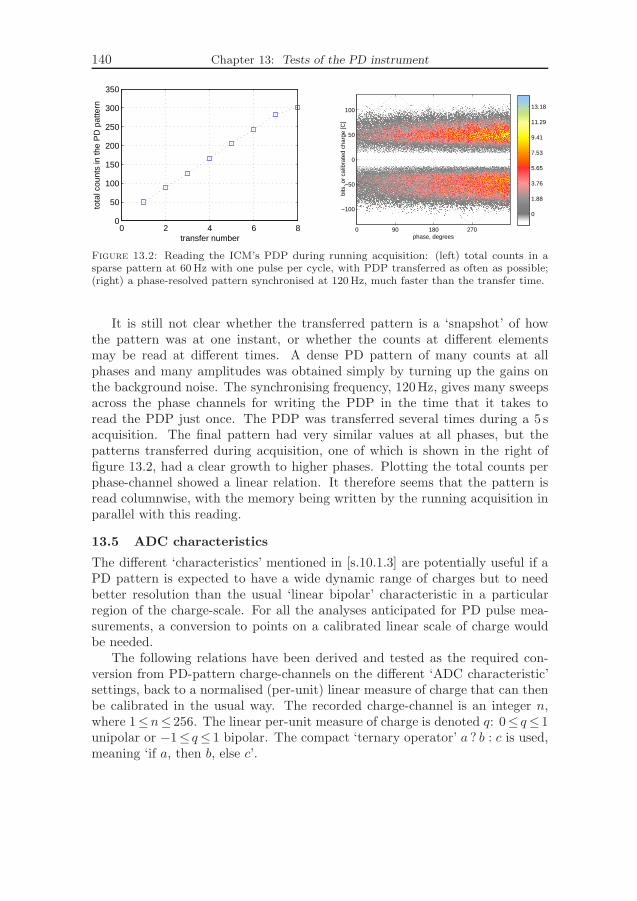
140 Chapter 13: Tests of the PD instrument
0 2 4 6 80
50
100
150
200
250
300
350
transfer number
tota
l cou
nts
in th
e P
D p
atte
rn
phase, degrees
bits
, or
calib
rate
d ch
arge
[C]
0 90 180 270
−100
−50
0
50
100
0
1.88
3.76
5.65
7.53
9.41
11.29
13.18
Figure 13.2: Reading the ICM’s PDP during running acquisition: (left) total counts in asparse pattern at 60 Hz with one pulse per cycle, with PDP transferred as often as possible;(right) a phase-resolved pattern synchronised at 120 Hz, much faster than the transfer time.
It is still not clear whether the transferred pattern is a ‘snapshot’ of howthe pattern was at one instant, or whether the counts at different elementsmay be read at different times. A dense PD pattern of many counts at allphases and many amplitudes was obtained simply by turning up the gains onthe background noise. The synchronising frequency, 120Hz, gives many sweepsacross the phase channels for writing the PDP in the time that it takes toread the PDP just once. The PDP was transferred several times during a 5 sacquisition. The final pattern had very similar values at all phases, but thepatterns transferred during acquisition, one of which is shown in the right offigure 13.2, had a clear growth to higher phases. Plotting the total counts perphase-channel showed a linear relation. It therefore seems that the pattern isread columnwise, with the memory being written by the running acquisition inparallel with this reading.
13.5 ADC characteristics
The different ‘characteristics’ mentioned in [s.10.1.3] are potentially useful if aPD pattern is expected to have a wide dynamic range of charges but to needbetter resolution than the usual ‘linear bipolar’ characteristic in a particularregion of the charge-scale. For all the analyses anticipated for PD pulse mea-surements, a conversion to points on a calibrated linear scale of charge wouldbe needed.
The following relations have been derived and tested as the required con-version from PD-pattern charge-channels on the different ‘ADC characteristic’settings, back to a normalised (per-unit) linear measure of charge that can thenbe calibrated in the usual way. The recorded charge-channel is an integer n,where 1≤n≤ 256. The linear per-unit measure of charge is denoted q: 0≤ q≤ 1unipolar or −1≤ q≤ 1 bipolar. The compact ‘ternary operator’ a ? b : c is used,meaning ‘if a, then b, else c’.
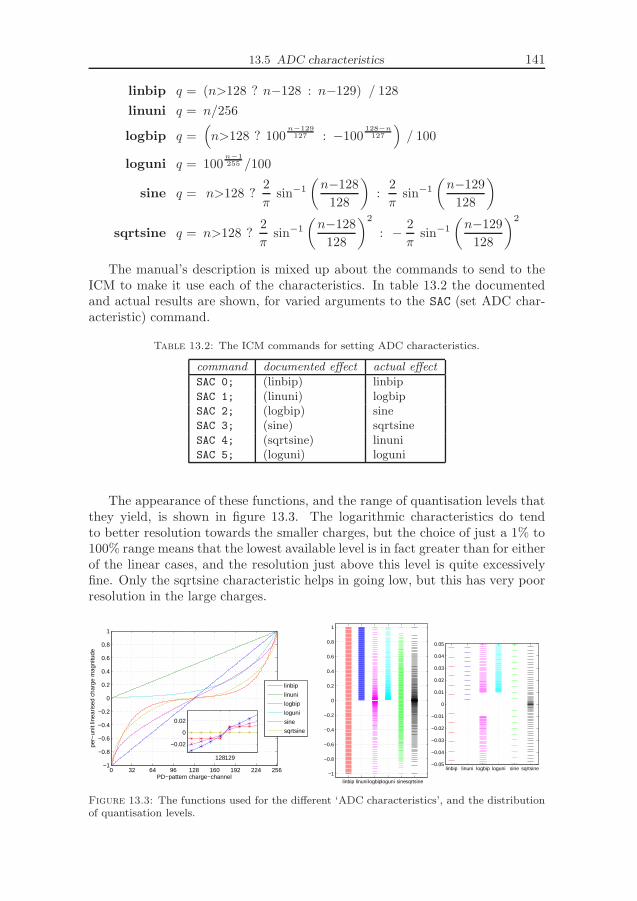
13.5 ADC characteristics 141
linbip q = (n>128 ? n−128 : n−129) / 128
linuni q = n/256
logbip q =(
n>128 ? 100n−129
127 : −100128−n
127
)
/ 100
loguni q = 100n−1
255 /100
sine q = n>128 ?2
πsin−1
(
n−128
128
)
:2
πsin−1
(
n−129
128
)
sqrtsine q = n>128 ?2
πsin−1
(
n−128
128
)2
: − 2
πsin−1
(
n−129
128
)2
The manual’s description is mixed up about the commands to send to theICM to make it use each of the characteristics. In table 13.2 the documentedand actual results are shown, for varied arguments to the SAC (set ADC char-acteristic) command.
Table 13.2: The ICM commands for setting ADC characteristics.
command documented effect actual effect
SAC 0; (linbip) linbipSAC 1; (linuni) logbipSAC 2; (logbip) sineSAC 3; (sine) sqrtsineSAC 4; (sqrtsine) linuniSAC 5; (loguni) loguni
The appearance of these functions, and the range of quantisation levels thatthey yield, is shown in figure 13.3. The logarithmic characteristics do tendto better resolution towards the smaller charges, but the choice of just a 1% to100% range means that the lowest available level is in fact greater than for eitherof the linear cases, and the resolution just above this level is quite excessivelyfine. Only the sqrtsine characteristic helps in going low, but this has very poorresolution in the large charges.
0 32 64 96 128 160 192 224 256−1
−0.8
−0.6
−0.4
−0.2
0
0.2
0.4
0.6
0.8
1
PD−pattern charge−channel
per−
unit
linea
rised
cha
rge
mag
nitu
de
linbip
linuni
logbip
loguni
sine
sqrtsine
128129
−0.02
0
0.02
linbip linuni logbiploguni sinesqrtsine
−1
−0.8
−0.6
−0.4
−0.2
0
0.2
0.4
0.6
0.8
1
linbip linuni logbip loguni sine sqrtsine−0.05
−0.04
−0.03
−0.02
−0.01
0
0.01
0.02
0.03
0.04
0.05
Figure 13.3: The functions used for the different ‘ADC characteristics’, and the distributionof quantisation levels.
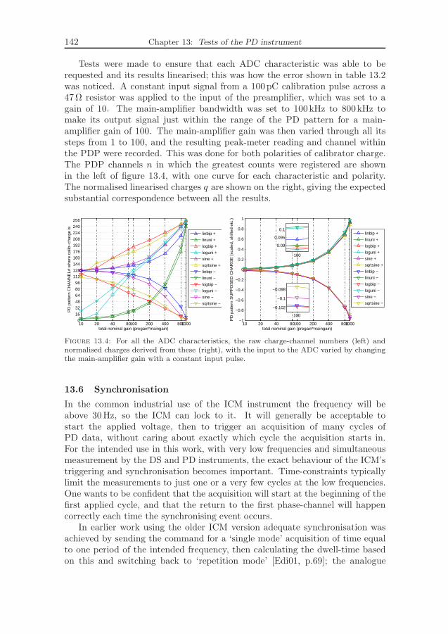
142 Chapter 13: Tests of the PD instrument
Tests were made to ensure that each ADC characteristic was able to berequested and its results linearised; this was how the error shown in table 13.2was noticed. A constant input signal from a 100pC calibration pulse across a47Ω resistor was applied to the input of the preamplifier, which was set to again of 10. The main-amplifier bandwidth was set to 100kHz to 800kHz tomake its output signal just within the range of the PD pattern for a main-amplifier gain of 100. The main-amplifier gain was then varied through all itssteps from 1 to 100, and the resulting peak-meter reading and channel withinthe PDP were recorded. This was done for both polarities of calibrator charge.The PDP channels n in which the greatest counts were registered are shownin the left of figure 13.4, with one curve for each characteristic and polarity.The normalised linearised charges q are shown on the right, giving the expectedsubstantial correspondence between all the results.
10 20 40 80100 200 400 80010000
16
32
48
64
80
96
112
128
144
160
176
192
208
224
240
256
total nominal gain (pregain*maingain)
PD
pat
tern
CH
AN
NE
L# w
here
cal
ib−
char
ge is
linbip +
linuni +
logbip +
loguni +
sine +
sqrtsine +
linbip −
linuni −
logbip −
loguni −
sine −
sqrtsine −
10 20 40 80100 200 400 8001000−1
−0.8
−0.6
−0.4
−0.2
0
0.2
0.4
0.6
0.8
1
total nominal gain (pregain*maingain)
PD
pat
tern
SU
PP
OS
ED
CH
AR
GE
(sc
aled
, shi
fted
etc.
)
linbip +
linuni +
logbip +
loguni +
sine +
sqrtsine +
linbip −
linuni −
logbip −
loguni −
sine −
sqrtsine −
100
0.09
0.095
0.1
100
−0.102
−0.1
−0.098
Figure 13.4: For all the ADC characteristics, the raw charge-channel numbers (left) andnormalised charges derived from these (right), with the input to the ADC varied by changingthe main-amplifier gain with a constant input pulse.
13.6 Synchronisation
In the common industrial use of the ICM instrument the frequency will beabove 30Hz, so the ICM can lock to it. It will generally be acceptable tostart the applied voltage, then to trigger an acquisition of many cycles ofPD data, without caring about exactly which cycle the acquisition starts in.For the intended use in this work, with very low frequencies and simultaneousmeasurement by the DS and PD instruments, the exact behaviour of the ICM’striggering and synchronisation becomes important. Time-constraints typicallylimit the measurements to just one or a very few cycles at the low frequencies.One wants to be confident that the acquisition will start at the beginning of thefirst applied cycle, and that the return to the first phase-channel will happencorrectly each time the synchronising event occurs.
In earlier work using the older ICM version adequate synchronisation wasachieved by sending the command for a ‘single mode’ acquisition of time equalto one period of the intended frequency, then calculating the dwell-time basedon this and switching back to ‘repetition mode’ [Edi01, p.69]; the analogue
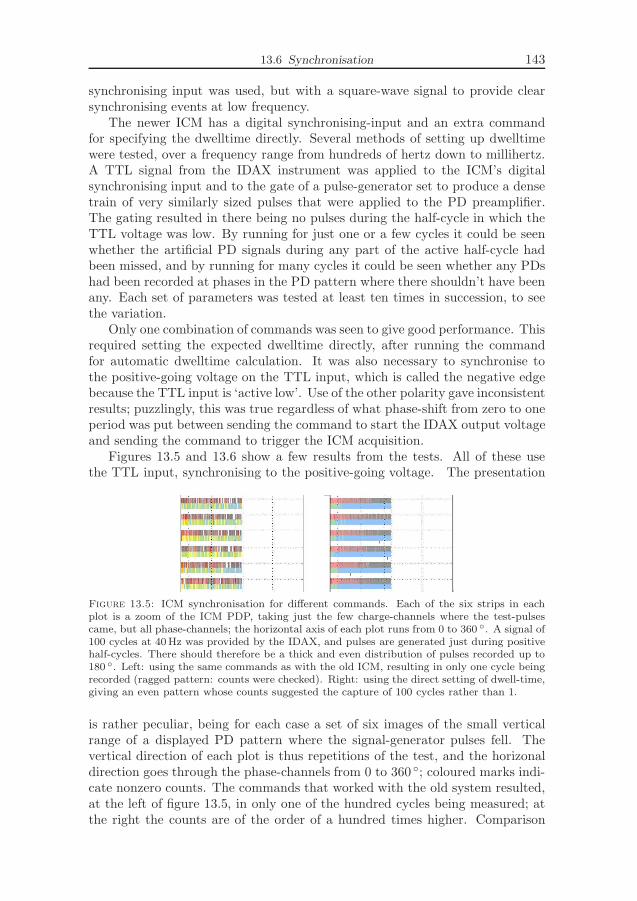
13.6 Synchronisation 143
synchronising input was used, but with a square-wave signal to provide clearsynchronising events at low frequency.
The newer ICM has a digital synchronising-input and an extra commandfor specifying the dwelltime directly. Several methods of setting up dwelltimewere tested, over a frequency range from hundreds of hertz down to millihertz.A TTL signal from the IDAX instrument was applied to the ICM’s digitalsynchronising input and to the gate of a pulse-generator set to produce a densetrain of very similarly sized pulses that were applied to the PD preamplifier.The gating resulted in there being no pulses during the half-cycle in which theTTL voltage was low. By running for just one or a few cycles it could be seenwhether the artificial PD signals during any part of the active half-cycle hadbeen missed, and by running for many cycles it could be seen whether any PDshad been recorded at phases in the PD pattern where there shouldn’t have beenany. Each set of parameters was tested at least ten times in succession, to seethe variation.
Only one combination of commands was seen to give good performance. Thisrequired setting the expected dwelltime directly, after running the commandfor automatic dwelltime calculation. It was also necessary to synchronise tothe positive-going voltage on the TTL input, which is called the negative edgebecause the TTL input is ‘active low’. Use of the other polarity gave inconsistentresults; puzzlingly, this was true regardless of what phase-shift from zero to oneperiod was put between sending the command to start the IDAX output voltageand sending the command to trigger the ICM acquisition.
Figures 13.5 and 13.6 show a few results from the tests. All of these usethe TTL input, synchronising to the positive-going voltage. The presentation
Figure 13.5: ICM synchronisation for different commands. Each of the six strips in eachplot is a zoom of the ICM PDP, taking just the few charge-channels where the test-pulsescame, but all phase-channels; the horizontal axis of each plot runs from 0 to 360 . A signal of100 cycles at 40Hz was provided by the IDAX, and pulses are generated just during positivehalf-cycles. There should therefore be a thick and even distribution of pulses recorded up to180 . Left: using the same commands as with the old ICM, resulting in only one cycle beingrecorded (ragged pattern: counts were checked). Right: using the direct setting of dwell-time,giving an even pattern whose counts suggested the capture of 100 cycles rather than 1.
is rather peculiar, being for each case a set of six images of the small verticalrange of a displayed PD pattern where the signal-generator pulses fell. Thevertical direction of each plot is thus repetitions of the test, and the horizonaldirection goes through the phase-channels from 0 to 360 ; coloured marks indi-cate nonzero counts. The commands that worked with the old system resulted,at the left of figure 13.5, in only one of the hundred cycles being measured; atthe right the counts are of the order of a hundred times higher. Comparison

144 Chapter 13: Tests of the PD instrument
Figure 13.6: ICM synchronisation for varied phase of triggering. The case in the centreis similar to the right of figure 13.5, but with just 1 cycle at 5 Hz. To the right there is ahalf-period delay between starting the IDAX and triggering the ICM. To the left the IDAXis simply left on and the ICM starts at arbitrary phase.
of delays between IDAX start and ICM trigger showed that even a half-cycledelay gave no problem, but there can be problems of wrong synchronisationwhen triggering the ICM at certain phases.
13.7 Linearity
A common definition of linearity of a function f(·) includes the condition thatf(ka) = kf(a); if negative k is permitted, so that k = −1 can be chosen, thena PD measurement system should record positive or negative calibration pulsesof similar magnitude as having the same magnitude, to within the system’spermitted degree of non-linearity.
The ICM does not make a direct claim of its linearity or polarity dependence,but is supposed to conform to IEC-60270. In that standard the most relevantparameter that must be tested for a PD measurement system is the scale factor,k. This is the ratio of the measured response to the size of the applied calibrationcharge; it should be taken at three or more calibration charge values rangingfrom 10% to 100% of the instrument’s full scale, and “the variation of k shallbe less than ± 5% in order to prove the linearity of the system”. A calibratoris tested by measuring its charge by a method with uncertainty no more thanthe greater of 5% or 1 pC. Putting these two criteria together implies a possible10% variation in linearity between 10% and 100% of scale of an approved PDmeasurement system.
A PD measurement system conforming to this standard may therefore havesubstantial differences, of some 10%, in its scale factor at different magnitudes,and it is not obvious what requirement there is on polarity-dependence. Areversal of calibrator leads is a simple way to compare the scale factor at oppositepolarities, with the advantage that the calibrator charge should in this case bevery consistent, thus avoiding bringing the calibrator’s permitted uncertaintyinto the measurement of scale factor.
In view of the usual noisiness and stochastic variation of PD measurements, a10% variation in scale factor may be acceptable for conventional industrial diag-nostics. When some of the results are expected to come from small laboratory-samples, to be compared with DS measurements of PD charge, and to beanalysed quite carefully, it becomes much more troublesome to have even afew percent of systematic error of magnitude with polarity. Assessment andcompensation of such errors should be tried.
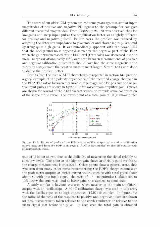
13.7 Linearity 145
The users of our older ICM system noticed some years ago that similar inputmagnitudes of positive and negative PD signals to the preamplifier can givedifferent measured magnitudes. From [For08a, p.25], “it was observed that forlow gains and steep input pulses the amplification factor was slightly differentfor positive and negative pulses”. In that work the problem was reduced byadapting the detection impedance to give smaller and slower input pulses, andby using quite high gains. It was immediately apparent with the newer ICMthat the background noise appeared sooner in the negative part of the PDPwhen the gain was increased or the LLD level (threshold) was decreased into thenoise. Large variations, easily 10%, were seen between measurements of positiveand negative calibration pulses that should have had the same magnitude; thevariation always made the negative measurement larger. Several tests were doneto define the problem better.
Results from the tests of ADC characteristics reported in section 13.5 providea good example of the polarity-dependence of the recorded charge-channels inthe PDP. The ratios between measured charge magnitude for positive and nega-tive input pulses are shown in figure 13.7 for varied main-amplifier gain. Curvesare shown for several of the ADC characteristics, to provide some confirmationof the shape of the curve. The lowest point at a total gain of 10 (main-amplifier
20 40 80 100 200 400 8001000
0.5
0.6
0.7
0.8
0.9
1.0
total nominal gain (pregain*maingain)
ratio
of +
/− r
espo
nse
in P
DP
linbip
logbip
sine
sqrtsine
Figure 13.7: Ratios of peaks of the ICM main-amplifier output to + and − calibrationpulses, measured from the PDP using several ‘ADC characteristics’ to give different spreadsof quantisation levels.
gain of 1) is not shown, due to the difficulty of measuring the signal reliably atsuch low levels. The point at the highest gain shows artificially good results asthe charge measurement is saturated. Other points show a general trend thatwas seen from many other measurements using the PDP’s charge channels orthe peak-meter output: at higher output values, such as with total gains aboveabout 80 with this input signal, the ratio of +/− magnitudes is about 5% to10% below the true ratio, and at lower gains this worsens to some 25%.
A fairly similar behaviour was seen when measuring the main-amplifier’soutput with an oscilloscope. A 50 pC calibration charge was used in this case,with the oscilloscope set to high-impedance (1 MΩ) dc-coupled. In figure 13.8the ratios of the peak of the response to positive and negative pulses are shownfor peak-measurement taken relative to the earth conductor or relative to themean signal just before the pulse. In each case the total gain is obtained
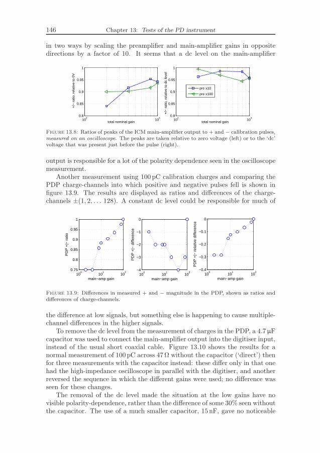
146 Chapter 13: Tests of the PD instrument
in two ways by scaling the preamplifier and main-amplifier gains in oppositedirections by a factor of 10. It seems that a dc level on the main-amplifier
102
103
0.8
0.85
0.9
0.95
1+
/− r
atio
, rel
ativ
e to
0V
total nominal gain
102
103
0.8
0.85
0.9
0.95
1
+/−
rat
io, r
elat
ive
to d
c le
vel
total nominal gain
pre x10
pre x100
Figure 13.8: Ratios of peaks of the ICM main-amplifier output to + and − calibration pulses,measured on an oscilloscope. The peaks are taken relative to zero voltage (left) or to the ‘dc’voltage that was present just before the pulse (right).
output is responsible for a lot of the polarity dependence seen in the oscilloscopemeasurement.
Another measurement using 100 pC calibration charges and comparing thePDP charge-channels into which positive and negative pulses fell is shown infigure 13.9. The results are displayed as ratios and differences of the charge-channels ±(1, 2, . . . 128). A constant dc level could be responsible for much of
100
101
102
0.75
0.8
0.85
0.9
0.95
1
main−amp gain
PD
P +
|− r
atio
100
101
102
−4
−3
−2
−1
0
main−amp gain
PD
P +
|− d
iffer
ence
100
101
102
−0.4
−0.3
−0.2
−0.1
0
main−amp gain
PD
P +
|− r
elat
ive
diffe
renc
e
Figure 13.9: Differences in measured + and − magnitude in the PDP, shown as ratios anddifferences of charge-channels.
the difference at low signals, but something else is happening to cause multiple-channel differences in the higher signals.
To remove the dc level from the measurement of charges in the PDP, a 4.7µFcapacitor was used to connect the main-amplifier output into the digitiser input,instead of the usual short coaxial cable. Figure 13.10 shows the results for anormal measurement of 100 pC across 47Ω without the capacitor (‘direct’) thenfor three measurements with the capacitor instead: these differ only in that onehad the high-impedance oscilloscope in parallel with the digitiser, and anotherreversed the sequence in which the different gains were used; no difference wasseen for these changes.
The removal of the dc level made the situation at the low gains have novisible polarity-dependence, rather than the difference of some 30% seen withoutthe capacitor. The use of a much smaller capacitor, 15 nF, gave no noticeable
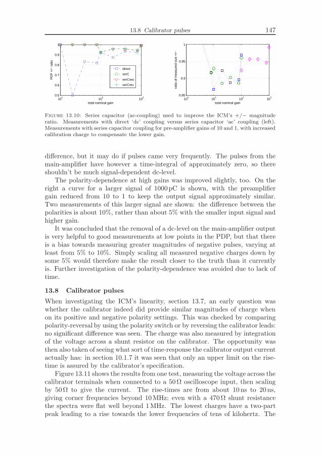
13.8 Calibrator pulses 147
101
102
103
0.5
0.6
0.7
0.8
0.9
1
total nominal gain
PD
P +
/− r
atio
direct
serC
serCosc
serCrev
100
101
102
103
0.85
0.9
0.95
1
total nominal gain
ratio
of m
easu
red
size
+/−
Figure 13.10: Series capacitor (ac-coupling) used to improve the ICM’s +/− magnituderatio. Measurements with direct ‘dc’ coupling versus series capacitor ‘ac’ coupling (left).Measurements with series capacitor coupling for pre-amplifier gains of 10 and 1, with increasedcalibration charge to compensate the lower gain.
difference, but it may do if pulses came very frequently. The pulses from themain-amplifier have however a time-integral of approximately zero, so thereshouldn’t be much signal-dependent dc-level.
The polarity-dependence at high gains was improved slightly, too. On theright a curve for a larger signal of 1000pC is shown, with the preamplifiergain reduced from 10 to 1 to keep the output signal approximately similar.Two measurements of this larger signal are shown: the difference between thepolarities is about 10%, rather than about 5% with the smaller input signal andhigher gain.
It was concluded that the removal of a dc-level on the main-amplifier outputis very helpful to good measurements at low points in the PDP, but that thereis a bias towards measuring greater magnitudes of negative pulses, varying atleast from 5% to 10%. Simply scaling all measured negative charges down bysome 5% would therefore make the result closer to the truth than it currentlyis. Further investigation of the polarity-dependence was avoided due to lack oftime.
13.8 Calibrator pulses
When investigating the ICM’s linearity, section 13.7, an early question waswhether the calibrator indeed did provide similar magnitudes of charge whenon its positive and negative polarity settings. This was checked by comparingpolarity-reversal by using the polarity switch or by reversing the calibrator leads:no significant difference was seen. The charge was also measured by integrationof the voltage across a shunt resistor on the calibrator. The opportunity wasthen also taken of seeing what sort of time-response the calibrator output currentactually has: in section 10.1.7 it was seen that only an upper limit on the rise-time is assured by the calibrator’s specification.
Figure 13.11 shows the results from one test, measuring the voltage across thecalibrator terminals when connected to a 50Ω oscilloscope input, then scalingby 50Ω to give the current. The rise-times are from about 10 ns to 20 ns,giving corner frequencies beyond 10MHz; even with a 470Ω shunt resistancethe spectra were flat well beyond 1MHz. The lowest charges have a two-partpeak leading to a rise towards the lower frequencies of tens of kilohertz. The

148 Chapter 13: Tests of the PD instrument
−0.01 0 0.01 0.02 0.03 0.04 0.05−0.1
−0.05
0
0.05
0.1signal s(t)
time [µs]
I [A
]
−0.01 0 0.01 0.02 0.03 0.04 0.05−2
0
2
4
6
8
10x 10
7 signal s(t) (current) / Qcal
time [µs]
I[A] /
Qca
l[C]
−0.01 0 0.01 0.02 0.03 0.04 0.05−1
−0.5
0
0.5
1x 10
−9 integrated s(t)
time [µs]
Q[C
]
−0.01 0 0.01 0.02 0.03 0.04 0.05−0.5
0
0.5
1
1.5integrated s(t) (charge) / Qcal
time [µs]
Q[C
] / Q
cal[C
]
101
102
103
104
105
10−7
10−6
10−5
10−4
10−3
amplitude spectrum |S(w)|
f [kHz]
I(f)
[A]
101
102
103
104
105
103
104
105
106
amplitude spectrum |S(w)| / Qcal
f [kHz]
I(f)
[A] /
Qca
l[C]
cal1d +1000pC d 50R
cal1d −1000pC d 50R
cal1d +200pC d 50R
cal1d −200pC d 50R
cal1d +20pC d 50R
cal1d −20pC d 50R
Figure 13.11: Pulse currents of ±(20, 200, 1000) pC from the CAL1D calibrator into 50Ω,(top left). The currents are integrated to charge (middle left), and transformed by FFT toamplitude spectra (bottom left). On the right the same plots are normalised by the calibrationcharge: the two at 20 pC are the ones that are have a slow double-pulse in time, and fall offfaster at high frequency; the two at 200 pC rise the fastest.
mid-range charges, 200 pC in this case, have the most ideal waveforms andspectra, but there is a general trend of sharper rises for negative pulses, seenwith other shunt resistances and charge settings. The total charge within thepulse nonetheless integrates to very similar values for all the polarities andmagnitudes, as seen in the plot of normalised integrated charge.
13.9 Signal limits
The combination of the gains of both amplifiers and the short-term integral ofthe input signal determines the signal at the main-amplifier output. Excessivevalues here are very obvious from saturation of the PDP charge-channels and thepeak-meter: it is not obvious whether a pulse registered at the highest charge

13.9 Signal limits 149
level is in fact within that level or is higher, but one should treat anything atthe highest level as suspicious. Saturation of the preamplifier will not be seenfrom the PDP. The limits of the preamplifier output were tested by applyingpositive or negative 1000pC calibration charges across a 47Ω resistor shuntingthe preamplifier’s input; the preamplifier gain was 100 and the main-amplifier’sgain was 8. An oscilloscope set to high-impedance (1 MΩ) was used to measurethe voltage at the preamplifier output, using ac-coupling, and at the main-amplifier output, using dc-coupling. The response to an input pulse at t = 0 isshown in figure 13.12.
−2 0 2 4 6 8 10−10
−5
0
5
10
15
time [µs]
sign
al [V
]
pre−amp out ± 2.5V limit
PDP and peak−meter ± 5V limit
− (pre)
+ (pre)
− (main)
+ (main)
Figure 13.12: ICM amplifier output signal limits, tested with excessive input signal and gain.

150 Chapter 13: Tests of the PD instrument

Chapter 14
Contribution of PD to the total DS current
The DS and PD methods of measuring PD apparent charge will give results withsome differences and some similarities. This chapter considers the relations ofthe two types of measurement to the ideal apparent charge value, and howthese relations are affected by features of the instruments and of practical test-objects. This is done by some theoretical considerations and measurements ofpulse-sources of controlled magnitude and phase.
14.1 Comparison of DS and PD results
A pulsive PD event in a test-object causes a rapid change in potential onthe object’s terminals, and a rapid pulse of current flowing in from shuntcapacitances in the external circuit.
A PD-pulse measurement ideally records the overall charge-injection into aterminal of the test object or a coupling capacitor, for each PD pulse separately[s.8.2]. It can have a high sensitivity to PD pulses, as it avoids the frequency-band close to the applied voltage, in which the currents from the capacitanceand conductance lie. It can register pulses separately, preserving the distinctionbetween a few large PDs or many small PDs.
A DS measurement ideally records all charge into a terminal of the test-object [s.6.2], including the current from smooth capacitance and conductance aswell as from pulsive or glow PD. The measured PD current is only an aggregatedvalue, combining all PD events that occurred within a particular range of thephase of the applied voltage.
To estimate the current due to the PD alone, the other currents must beestimated and subtracted. In an object with large capacitance and a smallproportion of volume contributing to PD events, the errors in this subtractionwill easily swamp meaningful results.
14.2 Measurement of pulsed currents
The DS system needs to be able to measure PD currents, which arise as sharppulses at the test-object. The trouble with pulsed currents and resistive feedbackhas already been mentioned: a resistance low enough to avoid electrometeroverload during pulses is likely to be too low to provide an acceptable signalduring the rest of the time, if the pulses make up much of the total measuredcurrent. Capacitive feedback would integrate the pulses, simply stepping thefeedback voltage a little for each pulse that comes in, but it has undesirablefeatures particularly where there is a significant dc term in the current.
An important property of the DS instrument if it is to be used to measure PDcharge is that the recorded DFT components should include all the charge intothe measurement terminal. It is not certain that this will be true: there could
151
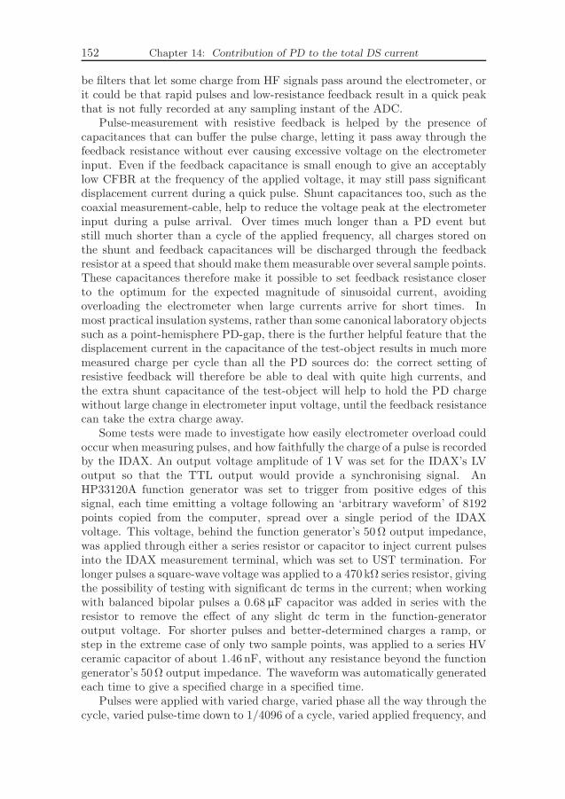
152 Chapter 14: Contribution of PD to the total DS current
be filters that let some charge from HF signals pass around the electrometer, orit could be that rapid pulses and low-resistance feedback result in a quick peakthat is not fully recorded at any sampling instant of the ADC.
Pulse-measurement with resistive feedback is helped by the presence ofcapacitances that can buffer the pulse charge, letting it pass away through thefeedback resistance without ever causing excessive voltage on the electrometerinput. Even if the feedback capacitance is small enough to give an acceptablylow CFBR at the frequency of the applied voltage, it may still pass significantdisplacement current during a quick pulse. Shunt capacitances too, such as thecoaxial measurement-cable, help to reduce the voltage peak at the electrometerinput during a pulse arrival. Over times much longer than a PD event butstill much shorter than a cycle of the applied frequency, all charges stored onthe shunt and feedback capacitances will be discharged through the feedbackresistor at a speed that should make them measurable over several sample points.These capacitances therefore make it possible to set feedback resistance closerto the optimum for the expected magnitude of sinusoidal current, avoidingoverloading the electrometer when large currents arrive for short times. Inmost practical insulation systems, rather than some canonical laboratory objectssuch as a point-hemisphere PD-gap, there is the further helpful feature that thedisplacement current in the capacitance of the test-object results in much moremeasured charge per cycle than all the PD sources do: the correct setting ofresistive feedback will therefore be able to deal with quite high currents, andthe extra shunt capacitance of the test-object will help to hold the PD chargewithout large change in electrometer input voltage, until the feedback resistancecan take the extra charge away.
Some tests were made to investigate how easily electrometer overload couldoccur when measuring pulses, and how faithfully the charge of a pulse is recordedby the IDAX. An output voltage amplitude of 1V was set for the IDAX’s LVoutput so that the TTL output would provide a synchronising signal. AnHP33120A function generator was set to trigger from positive edges of thissignal, each time emitting a voltage following an ‘arbitrary waveform’ of 8192points copied from the computer, spread over a single period of the IDAXvoltage. This voltage, behind the function generator’s 50Ω output impedance,was applied through either a series resistor or capacitor to inject current pulsesinto the IDAX measurement terminal, which was set to UST termination. Forlonger pulses a square-wave voltage was applied to a 470kΩ series resistor, givingthe possibility of testing with significant dc terms in the current; when workingwith balanced bipolar pulses a 0.68µF capacitor was added in series with theresistor to remove the effect of any slight dc term in the function-generatoroutput voltage. For shorter pulses and better-determined charges a ramp, orstep in the extreme case of only two sample points, was applied to a series HVceramic capacitor of about 1.46 nF, without any resistance beyond the functiongenerator’s 50Ω output impedance. The waveform was automatically generatedeach time to give a specified charge in a specified time.
Pulses were applied with varied charge, varied phase all the way through thecycle, varied pulse-time down to 1/4096 of a cycle, varied applied frequency, and
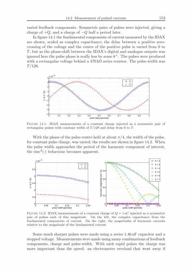
14.2 Measurement of pulsed currents 153
varied feedback components. Symmetric pairs of pulses were injected, giving acharge of +Q, and a charge of −Q half a period later.
In figure 14.1 the fundamental components of current measured by the IDAXare shown, scaled as complex capacitance; the delay between a positive zero-crossing of the voltage and the centre of the positive pulse is varied from 0 toT , but as the phase-shift between the IDAX’s digital and analogue outputs wasignored here the pulse phase is really less by some 8 . The pulses were producedwith a rectangular voltage behind a 470 kΩ series resistor. The pulse-width wasT/128.
0 0.1 0.2 0.3 0.4 0.5 0.6 0.7 0.8 0.9 1−4
−3
−2
−1
0
1
2
3
4x 10
−10
pulse delay [periods]
C’ &
C’’
[F]
C’
C’’
Figure 14.1: IDAX measurements of a constant charge injected as a symmetric pair ofrectangular pulses with constant width of T/128 and delay from 0 to T .
With the phase of the pulse-centre held at about π/4, the width of the pulse,for constant pulse charge, was varied; the results are shown in figure 14.2. Whenthe pulse width approaches the period of the harmonic component of interest,the sinc2(·) behaviour becomes apparent.
0 0.05 0.1 0.15 0.2 0.253
3.5
4
4.5
5
5.5
x 10−10
pulse width [periods]
C’ &
C’’
[F]
C’C’’
0 0.05 0.1 0.15 0.2 0.250
0.2
0.4
0.6
0.8
1
pulse width [periods]
harm
onic
mag
nitu
de (
rel.
h1)
h = 2
h = 3
h = 4
h = 5
h = 6
h = 7
Figure 14.2: IDAX measurements of a constant charge of Q = 1nC injected as a symmetricpair of pulses each of this magnitude. On the left, the complex capacitance from thefundamental components of current. On the right, the magnitudes of harmonic currentsrelative to the magnitude of the fundamental current.
Some much sharper pulses were made using a series 1.46nF capacitor and astepped voltage. Measurements were made using many combinations of feedbackcomponents, charge and pulse-width. With such rapid pulses the charge wasmore important than the speed: an electrometer overload that went away if
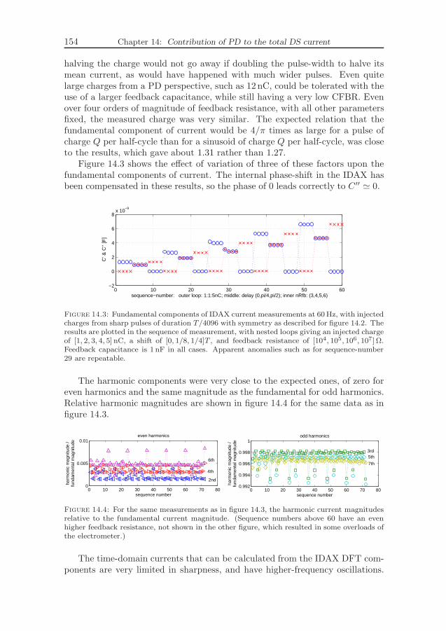
154 Chapter 14: Contribution of PD to the total DS current
halving the charge would not go away if doubling the pulse-width to halve itsmean current, as would have happened with much wider pulses. Even quitelarge charges from a PD perspective, such as 12 nC, could be tolerated with theuse of a larger feedback capacitance, while still having a very low CFBR. Evenover four orders of magnitude of feedback resistance, with all other parametersfixed, the measured charge was very similar. The expected relation that thefundamental component of current would be 4/π times as large for a pulse ofcharge Q per half-cycle than for a sinusoid of charge Q per half-cycle, was closeto the results, which gave about 1.31 rather than 1.27.
Figure 14.3 shows the effect of variation of three of these factors upon thefundamental components of current. The internal phase-shift in the IDAX hasbeen compensated in these results, so the phase of 0 leads correctly to C′′ ≃ 0.
0 10 20 30 40 50 60−2
0
2
4
6
8x 10
−9
sequence−number: outer loop: 1:1:5nC; middle: delay (0,pi/4,pi/2); inner nRfb: (3,4,5,6)
C’ &
C’’
[F]
Figure 14.3: Fundamental components of IDAX current measurements at 60 Hz, with injectedcharges from sharp pulses of duration T/4096 with symmetry as described for figure 14.2. Theresults are plotted in the sequence of measurement, with nested loops giving an injected chargeof [1, 2, 3, 4, 5] nC, a shift of [0, 1/8, 1/4]T , and feedback resistance of [104, 105, 106, 107] Ω.Feedback capacitance is 1 nF in all cases. Apparent anomalies such as for sequence-number29 are repeatable.
The harmonic components were very close to the expected ones, of zero foreven harmonics and the same magnitude as the fundamental for odd harmonics.Relative harmonic magnitudes are shown in figure 14.4 for the same data as infigure 14.3.
0 10 20 30 40 50 60 70 800
0.005
0.01
sequence number
harm
onic
mag
nitu
de /
fund
amen
tal m
agni
tude
even harmonics
0 10 20 30 40 50 60 70 800.992
0.994
0.996
0.998
1
sequence number
odd harmonics
harm
onic
mag
nitu
de /
fund
amen
tal m
agni
tude
6th
4th
2nd
3rd
7th
5th
Figure 14.4: For the same measurements as in figure 14.3, the harmonic current magnitudesrelative to the fundamental current magnitude. (Sequence numbers above 60 have an evenhigher feedback resistance, not shown in the other figure, which resulted in some overloads ofthe electrometer.)
The time-domain currents that can be calculated from the IDAX DFT com-ponents are very limited in sharpness, and have higher-frequency oscillations.
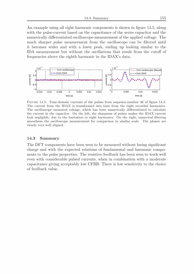
14.3 Summary 155
An example using all eight harmonic components is shown in figure 14.5, alongwith the pulse-current based on the capacitance of the series capacitor and thenumerically differentiated oscilloscope-measurement of the applied voltage. Themuch sharper pulse measurement from the oscilloscope can be filtered untilit becomes wider and with a lower peak, ending up looking similar to theIDA measurement but without the oscillations that result from the cutoff offrequencies above the eighth harmonic in the IDAX’s data.
0 0.005 0.01 0.015−1
−0.5
0
0.5
1x 10
−5
time [s]
curr
ents
[A]
−0.015 −0.01 −0.005 0 0.005 0.01 0.015−1
−0.5
0
0.5
1x 10
−3
time [s]
curr
ents
[A]
from oscilloscope
from IDAXfrom oscilloscope (filtered)
from IDAX
Figure 14.5: Time-domain currents of the pulses from sequence-number 46 of figure 14.3.The current from the IDAX is transformed into time from the eight recorded harmonics.The oscilloscope measured voltage, which has been numerically differentiated to calculatethe current in the capacitor. On the left, the sharpness of pulses makes the IDAX currentlook negligible, due to the limitation to eight harmonics. On the right, numerical filteringsmoothens the oscilloscope measurement for comparison in similar scale. The phases areclearly very well aligned.
14.3 Summary
The DFT components have been seen to be measured without losing significantcharge and with the expected relations of fundamental and harmonic compo-nents to the pulse properties. The resistive feedback has been seen to work welleven with considerable pulsed currents, when in combination with a moderatecapacitance giving acceptably low CFBR. There is low sensitivity to the choiceof feedback value.

156 Chapter 14: Contribution of PD to the total DS current

Chapter 15
Processing and display of DS and PD results
The types of measurements being studied here produce many times as much dataas the conventional diagnostic measurements made on stator insulation. Thestoring, processing and presenting of results thus becomes especially importantif patterns and frequency dependence are to be noticed. This chapter considerswhat extra data the proposed methods produce, and suggests ways of presentingit.
15.1 Conventional measurements and presentation
Even the conventional offline electrical diagnostic measurements for stator insu-lation can generate enough data to need some attention to good forms of display,particularly for comparison and trending.
The time-domain measurements of IR and PI [s.6.4.2] can be recorded asa time-series or as a single number at a specified time. The single-frequencymeasurements of C-tan δ [s.6.4.1] are usually made at several voltages, recordingjust the pair of fundamental-frequency results at each.
Most modern PD measurements are based on a PRPDA method [s.8.2.4]where counts are recorded in a matrix of thousands of combinations of pulsemagnitude and phase of occurrence; the measurement is generally made oversame range of voltage levels as for C-tan δ [s.8.5]. The total information canthus be a great deal more than for the other measurements, and many waysare used of reducing the PDP to a function of one variable [s.8.2.4]. ThePD measurements are clearly much the most data-intensive of the conventionalmethods.
Provided that the neutral point can be split, all of these measurements canbe performed separately on each phase and then on all phases together [s.4.5],which increases the data by a factor of four. Separate measurements of PD atthe phase end and neutral end [s.8.5] can further double the resulting data.
15.2 Further data from the proposed measurements
The methods studied in this work increase the amount of data from eachmeasurement in several ways: harmonics are included in DS measurements,PD pulse measurements are interpreted in the form of currents as well as theusual patterns and indices, and multiple frequencies are used.
The DS results include the harmonics of voltage and current; the harmonicsup to the eighth are included by the present instrument. The scope of this workis limited to applied voltages that are intended to be sinusoidal: harmonics inthe voltage are only measured in order to correct the measured current. TheDS data that must be presented is therefore only based on current harmonics.
157

158 Chapter 15: Processing and display of DS and PD results
The data from a DS measurement is increased by several times by includingharmonics, but it is still much less than the raw PD data.
The PD results are a conventional PR-PDP for each point; from the presentinstrument the size is 256×256 elements. This can be studied by the conven-tional features such as pattern and maximum charge, and also as the waveformof mean current due to the measured charges, for comparison on similar termswith the DS results. For a winding rather than a single bar in the lab, thecalibration of the pulses to true apparent charge is not possible [s.8.4], but acomparison of the waveform’s shape might still be desired.
The DS and PD measurements are made over many frequencies as well asover the several voltages that are conventional. At least two decades of frequencyare likely to be included in a seriously ‘variable frequency’ measurement, evenwhen measuring on industrial equipment in the field. Several points per decadeshould be taken if trends are to be clearly seen. For a test-object with acapacitance of the hundreds of nanofarads typical for a stator phase, an upperlimit of about 1Hz is likely at high voltage, due to limitations of the voltageamplifier. To keep the measurement-time reasonable when working at severalvoltages and on separate and combined phases, a lower limit of about 10mHz islikely to be needed. In the laboratory with smaller objects and longer availabletime, five decades from 100Hz to 1mHz may be studied even at high voltage.Varying the frequency therefore results in at least a five times increase in datacompared to single-frequency measurements, and possibly twenty or more timesin a laboratory situation.
15.3 Suggested presentation
If a single number can be used to represent the results at each combination ofamplitude and frequency (each point), a good way of plotting the whole mea-surement is to plot a curve against frequency for each amplitude. This is usuallypreferable to plotting against amplitude: there are usually more frequencypoints than amplitude points, and the shape of the curve against frequencyis generally of more interest than curves against amplitude, particularly for DSmeasurements on largely linear objects. Variable-frequency methods that havebeen applied in other types of insulation such as cables [s.6.3] have done thiswith two numbers, representing the complex capacitance at each point as C′
and C′′ or as C-tan δ . It would be good to be able to represent the harmonicsin DS, and important features of PR-PDPs, as also just a few numbers that canbe plotted in this way.
15.3.1 PD patterns
A single PR-PDP is already a complicated three-dimensional data-set, poten-tially holding a large amount of information. There is no direct substitute forlooking at every pattern and seeing the variation with the controlled variables;no small set of indices would make clear the changes in pattern seen betweendifferent frequencies in for example [Cav06].
There may easily be tens of acquired PD patterns for a measurement withvaried amplitude and frequency, even when only on one object such as a partic-ular phase. It may be worth sacrificing or supplementing the high level of detail

15.3.2 DS including harmonics 159
of a PR-PDP in order to get the benefit of seeing a comparison of frequencyand amplitude dependence all in one plot.
Reduction to one of the many conventional indices such as mean or maximumcharge can be used to enable a single plot to display of some feature of all themeasured points. Such indices, although derived from a PDP, are in a way asource of extra information as well as a way of reducing the data, since they canshow trends that the eye would not notice so clearly. As an example, admittedlynot with real PD, the strong linearity in figure 13.2 [p.140] was much moreobvious when each pattern was reduced to total counts and plotted than whenmerely looking at a sequence of patterns.
Conversion of a PR-PDP to the mean PD current reduces the charge mag-nitude and count dimensions into one, reducing the amount of detail but stillleaving a number at each of the phase-channels, 256 for the present instrument,rather than the desired single or few indices. One unconventional way of furtherreducing this current, which makes a lot of sense for the combined DS and PDmeasurements considered here, is to treat it in the same way as the DS current,converting it to its fundamental and low harmonics. The same methods ofdisplay can be used as for DS.
Some examples of reduction of PD data for plotting of frequency-dependenceare use of counts per cycle and mean charge in [For08b, fig.5], and a complex-capacitance description of the fundamental component of mean PD current in[Tay07]. For comparison of PD currents measured by DS and by the meancurrent from pulse measurements, [Edi01, ch.4] presents harmonic componentsin rectangular form; this is at a single frequency, but is nevertheless a DS-likeview of PD mean current rather than one of the conventional indices.
It is expected that a few conventional indices, possibly along with DS rep-resentations of mean current, will be a suitable compromise of sufficient infor-mation and not too many plots. It is important to be able to choose differentindices easily, and to see the full PD patterns if wanted.
15.3.2 DS including harmonics
For conventional frequency-domain dielectric spectroscopy, studying only thefundamental-frequency components, the measured current is usually presentedas a complex capacitance (6.1). This has some useful properties for measure-ments on insulation systems.
Division of the current’s amplitude by the voltage amplitude and frequencygives a constant value if the test-object is a pure, linear, dispersion-free ca-pacitor. The effects of dispersion and nonlinearity are then much more clearlynoticed and interpreted than they would be in the current, which due to thedominantly capacitive nature of good insulation would change approximately inproportion to frequency. This is the usual principle of scaling data towards aconstant, to see the variations clearly A.1.5.
The current’s phase is taken relative to the applied voltage, making clearthe relation of energy storage and dissipation components of the current at thefundamental-frequency.
The further ratio of these components of the current, to give tan δ (5.8),can be used to remove the effect of geometric capacitance, permitting more

160 Chapter 15: Processing and display of DS and PD results
direct comparison of different test-objects. (This work has instead focused onthe separate components C′ and C′′, partly because the division of rectangularparts of the current is a natural way to consider the stress-grading current andthe effects of PD, as well as to see the features of the power-law response of theepoxy-mica material.)
Having accepted this conventional presentation of fundamental current asthe indices C′ and C′′, one wonders if the harmonic currents can be treated in asimilar way. The magnitude of fundamental current in a largely capacitive test-object can vary by many orders of magnitude over a sweep of voltage amplitudeand frequency, and the harmonic currents may easily vary to the same degree.Indeed, it is likely they will vary more, as the expected nonlinearities in statorinsulation have typically a higher admittance at higher voltage; it is also likelythat the frequency-dependence will be strong, as with the fundamental current,since the current in most nonlinear parts of the construction, apart from cracksor leakage from the terminals, has a capacitance in series.
Some sort of scaling of harmonic currents by voltage amplitude and frequencyis therefore desirable. In the measurements considered in this work, only thefundamental component of applied voltage V1 is intended to be nonzero. Ap-proximate currents due to voltage harmonics Vn 6= 0 will have been subtractedfrom the measured current. The only voltage by which a harmonic currentcan meaningfully be divided is thus the fundamental. A suitable frequencyused for scaling the nth current-harmonic In could be argued to be either thefundamental frequency f or the harmonic frequency nf .
The harmonic current magnitude scaled in this way is
|Cn| =
∣
∣
∣
∣
In
ωV1
∣
∣
∣
∣
=
∣
∣
∣
∣
In
I1C1
∣
∣
∣
∣
(15.1)
which will be denoted Cn, the ‘harmonic capacitance’. This |Cn| is suitablefor plotting along with C1, typically being one or a few decades less for lowharmonics in a quite nonlinear object.
A still simpler form is to use just the relative magnitude of the harmoniccurrent to the fundamental current, which makes it easy to consider how dra-matically the harmonic would affect the current-waveform, without having tosee the fundamental capacitance as well,
|Inrel| =
∣
∣
∣
∣
In
I1
∣
∣
∣
∣
(15.2)
The phase, however, is critical to how a harmonic modifies the currentwaveform. Due to the mixture of capacitive and conductive currents harmonicswill not always cause an increase of the peak of the fundamental; their phasecannot be assumed. There are many possible choices of how best to presentcurrent-harmonics’ phase. It could be taken relative to the fundamental voltage,as is done for calculation of capacitance from fundamental current: but no clearrelevance such as the distinction of energy storage and loss in C′ and C′′ wouldcome from this. The relation to fundamental current is more relevant: similarlyto use of relative magnitude, it helps one to visualise the effect on the current

15.3.2 DS including harmonics 161
waveform. Remaining questions are then whether shifts between zero-crossingsor peaks of the fundamental and harmonic should be used, and whether the theseshifts should be expressed in terms of fundamental phase φ or harmonic phasenφ. Based on some experience with plotting these quantities for stress-gradingsamples, stress-gradings and PD, the harmonic phase-difference between peakshas been preferred.
The choice of plotting relative magnitudes was initially quite obvious. Hav-ing decided on the less obvious choice of phase, the question arises of whether arectangular form would be preferable. This is the preferred way for the funda-mental components, but there the distinction of energy storage and dissipationis significant. No harmonic will dissipate energy together with the fundamentalvoltage.
To plot all seven available harmonics would cause troublesome proliferationof data, at least when plotting with several voltage levels together. For sym-metrical objects the use of just odd harmonics, sometimes omitting the seventhas being small and noisy, is a natural way to reduce the data. A check can bemade that the even orders are much smaller than the third.
Other methods combine several harmonics into a single value, such as thetotal harmonic distortion (THD) [Pau92] widely used to describe limits of wave-form distortion for electrical equipment, or harmonic loss quality (HLQ) [Gof98]proposed as a measure of stator insulation condition. These have not beenexamined here, as the main desire is to visualise how a waveform or degree ofnonlinearity varies with frequency and voltage; the harmonic order and phasemust be preserved for this.
The third harmonic magnitude alone gives a good indication of the presenceof nonlinearity, and it is unlikely that higher-order harmonics would be consid-erably larger than the third harmonic in the sorts of waveform expected fromstator insulation.

162 Chapter 15: Processing and display of DS and PD results
Chapter 16
Effects of previous excitation on results
Interpretation of measurements usually involves comparisons. It is necessary tohave an estimate of how much variation can be expected in the results due tocauses other than fixed differences between test-objects or different measurementoccasions. Here, attention is given mainly to how a particular test-object duringone measurement may give varied results depending on its recent treatment,such as for example the order in which measurements are made. When usingmultiple amplitudes and frequencies this becomes particularly important.
16.1 Physical-system properties of stator insulation
The classic easy system for analysis in signals and control engineering is one thatis static, linear, time-invariant and deterministic. Of the phenomena of interestin this work, none possesses all of these simplifying features, and some possessnone of them! The dynamic nature of DR and PD phenomena, compoundedby some of the other deviations from the easy system, make the results ofmeasurements be dependent not only on the state of the insulation due to long-term irreversible aging that diagnostic measurements seek to determine, butalso on the state due to other parameters and recent treatment such as theambient temperature, the time since being in operation, and even the mostrecently applied stimuli used in the diagnostic measurement itself.
Being static implies that no knowledge of the past is needed to determinethe present. When this is not true, a system is dynamic, having some sortof statefulness that preserves information; the initial condition of the dynamicstate is needed in order to determine the response to an input. A simple exampleis the series RC circuit excited by a voltage source, where knowledge of thevoltage on the capacitor is needed in order to determine the current into thecircuit; the dynamic state is here linked to the energy stored in the capacitor,which depends on the history of the applied voltage to the circuit. A dielectricresponse function describes how the state imposed by electric fields throughoutthe history of the dielectric affects the polarisation at later times; the singlenumber that sufficed to describe the initial conditions of the RC circuit is notsufficient to describe this polarisation state for the general case of a responsefunction more complex than the Debye model. For PD the situation is far morecomplex, with many states that may significantly affect and be affected by PD:the temperature in a cavity’s gas and surroundings, the presence in the gas ofchemicals from surrounding surfaces, the density of electrons and ions in thegas or electrons trapped at surfaces. . . .
Being linear implies the validity of scaling and superposition: if an inputsignal can be represented as a sum of signals then the output is the sum of
163

164 Chapter 16: Effects of previous excitation on results
the outputs for all of these signals. This makes possible the use of frequency-based rather than time-based analyses, studying any applied signal as a sum ofsinusoids analysed independently. Only dielectric response of certain types ofmaterial at moderate fields can be said to be linear. Linearity is a reasonableassumption for the solid material of stator insulation at voltages below PDinception; it is certainly not true for PD phenomena, nor is it for stress-gradingaround the end-windings.
Being time-invariant implies constant parameters. A time-variant parametermight be seen as making up for a lack of detail in one’s model of the system:time-invariance can only be claimed if the model includes enough externaldisturbing parameters such as temperature changes, and enough internal statevariables such as self-induced temperature changes due to loss.
Being deterministic implies that in the presence of the same stimuli, the sameinitial conditions of dynamic state, and the same values of any time-dependentparameters, the same outputs will result. This is a very desirable propertyfor permitting the effect of a controlled variable to be seen; one would like tobe confident that two measurements with variation of just that variable, willproduce results whose difference is due purely to the controlled variable and notto a lack of determinism. Physical systems will have noise in the knowledgeof the ‘input’ conditions and the measurement of output, but in some casesthe variation is of very little practical importance. At the macroscopic level ofour models of DR, deterministic behaviour is a reasonable approximation, butbehind a sometimes strong background of measurement noise and dependenceon other factors such as statefulness. At the microscopic level of a single PDevent, the crucial occurrence of an initiating electron by external natural causescan only be seen as non-deterministic (stochastic). The aggregation of manysuch events, in for example a specimen with thousands of cavities and withmeasurements made over thousands of cycles, serves to reduce the extremity ofvariation due to stochastic processes. Even within a PD object that is excitedfor long periods with a constantly repeating signal, changes in the PD behaviourcan be seen [VB93][VB95][Lin09, p.65] on a timescale much more than a singlecycle of the excitation.
16.2 Standard measurement practice
The dependence of DR and PD measurements on previous treatment and dis-turbing parameters such as temperature is recognised in standard measurementpractice.
Time-domain dielectric response measurement by PDC [p.56] requires a longperiod of polarisation before depolarisation, or vice versa; the material’s initialstate must have come close to its equilibrium for all the timescale of the dielectricresponse function that is to be measured. For the ‘IR’ tests often made onstator insulation a discharging time at least four times the charging time isrecommended between subsequent measurements [E43, p.12].
Frequency-domain dielectric spectroscopy sometimes delays measuring thecurrent until the voltage has been applied for some cycles, in order that thematerial and measurement circuit should give currents close to the expected

16.3 Varied amplitude and frequency 165
equilibrium values as if the excitation had been applied for a long time before.The sequence of applied voltages normally used by the product family of theDS instrument used in this work goes up in amplitude, and down in frequencyat each amplitude, which reduces the disturbance of the excitation on the nextmeasurement.
The widely used power-frequency ‘tip-up’ tests are recommended [E286] tohave test voltages of increasing amplitude, to be preceded by a conditioningperiod where an excitation close to the maximum voltage of the test is appliedfor some 20 s to 240 s, and not to be preceded by a ‘hi-pot’ test. For newlymanufactured stator insulation that has not experienced PD, the conditioning(sometimes called a ‘soak’) not only warms up the insulation closer to thetemperature it will achieve during the measurement, but also changes pris-tine cavities by generating PD that increases the surface conductivity and theionisation in the gas [Eme05].
PD pulse measurements are often preceded by conditioning of the test objectby exciting it with a voltage possibly even higher than that intended for themeasurement. This can be done to make internal PD sources in a pristine test-object reach a relatively steady behaviour as in [For08a, p.29] or in the soakmentioned above for tip-up tests. It can be done for a shorter time to getthe PD in an aged test-object to be a better approximation of the PD duringsustained voltage application, for which [C3427, p.55] recommends five minutesat the highest test voltage. Steps in voltage amplitude should be held for some10 s to get a reliable PD pattern [C3427, p.57].
“Mechanical, thermal and electrical stressing just before the test can affectthe result of partial discharge tests. To ensure good reproducibility, a restinterval after previous stressing may be necessary before making partialdischarge tests.”[C270, clause 8.2]
16.3 Varied amplitude and frequency
The relevance of these complicating features of DR and PD to the types ofmeasurement considered in this work, where the excitation is a voltage withvaried amplitude and frequency, is how best to condition the specimens andselect the order, timing and repetition of the amplitude-frequency (V -f) pointsin order to get a suitable trade-off of measurement speed against usefulness ofthe result.
Measurements motivated by scientific interest in the physical phenomena,such as the modelling of PD in [For08a], will probably be aimed at results thatbest approximate the values one would obtain after either having had an appliedvoltage of the same amplitude and frequency for a long time, or having had noapplied voltage for a long time. The notion of steady state is qualified here by‘relatively’ because PD can vary so much even during long periods of constantexcitation. There will always be some degree of noise in a measurement, butPD sources are particularly extreme in their noisy variation and in that theycan show short and longer term changes and cycles.
Measurements for condition assessment do not so obviously require resultsthat reflect ‘equilibria’. The important link is the one between measurement
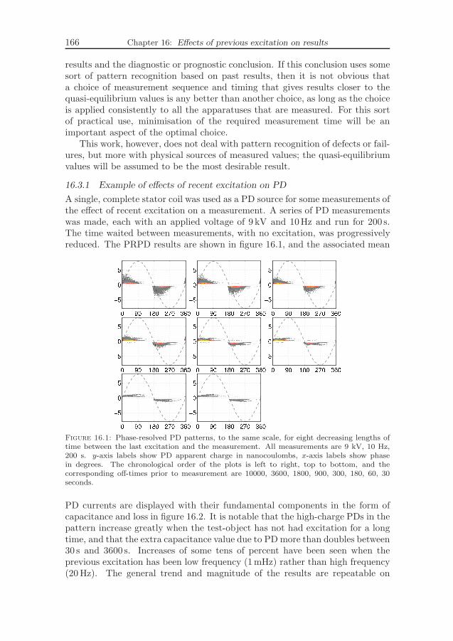
166 Chapter 16: Effects of previous excitation on results
results and the diagnostic or prognostic conclusion. If this conclusion uses somesort of pattern recognition based on past results, then it is not obvious thata choice of measurement sequence and timing that gives results closer to thequasi-equilibrium values is any better than another choice, as long as the choiceis applied consistently to all the apparatuses that are measured. For this sortof practical use, minimisation of the required measurement time will be animportant aspect of the optimal choice.
This work, however, does not deal with pattern recognition of defects or fail-ures, but more with physical sources of measured values; the quasi-equilibriumvalues will be assumed to be the most desirable result.
16.3.1 Example of effects of recent excitation on PD
A single, complete stator coil was used as a PD source for some measurements ofthe effect of recent excitation on a measurement. A series of PD measurementswas made, each with an applied voltage of 9 kV and 10Hz and run for 200 s.The time waited between measurements, with no excitation, was progressivelyreduced. The PRPD results are shown in figure 16.1, and the associated mean
Figure 16.1: Phase-resolved PD patterns, to the same scale, for eight decreasing lengths oftime between the last excitation and the measurement. All measurements are 9 kV, 10 Hz,200 s. y-axis labels show PD apparent charge in nanocoulombs, x-axis labels show phasein degrees. The chronological order of the plots is left to right, top to bottom, and thecorresponding off-times prior to measurement are 10000, 3600, 1800, 900, 300, 180, 60, 30seconds.
PD currents are displayed with their fundamental components in the form ofcapacitance and loss in figure 16.2. It is notable that the high-charge PDs in thepattern increase greatly when the test-object has not had excitation for a longtime, and that the extra capacitance value due to PD more than doubles between30 s and 3600 s. Increases of some tens of percent have been seen when theprevious excitation has been low frequency (1mHz) rather than high frequency(20 Hz). The general trend and magnitude of the results are repeatable on

16.4 Recommendation for swept measurements 167
Figure 16.2: PD charges of the patterns shown in figure 16.1, shown as C′ and C′′. Theorder of measurement was with longest off-time first.
the same object, implying that the mechanisms of the statefulness is not justirreversible aging.
16.4 Recommendation for swept measurements
The choice of sequence for sweeping across multiple voltage amplitudes andfrequencies is already established for the IDAX instrument and earlier versionsas going up in amplitude, and on each amplitude going down in frequency.Among the possibilities for the simple cases where each desired point is measuredwithout any waiting or other excitation in between, this choice does seem to bethe best. For the relatively simple case of DS, the increasing amplitude makesresidual polarisation be smaller relative to the measured point than it would bewith decreasing amplitude. For PD measurement the effect of long polarisationmay have stronger influence on a subsequent measurement at a high frequency:the linearity that simplifies treatment of DS measurements on solid insulatorscannot then be assumed. Depending on the test object, the measurement ofresults that correspond well to long-time application of a particular voltageamplitude and frequency may require a considerable period of that type ofexcitation before measurement.

168 Chapter 16: Effects of previous excitation on results
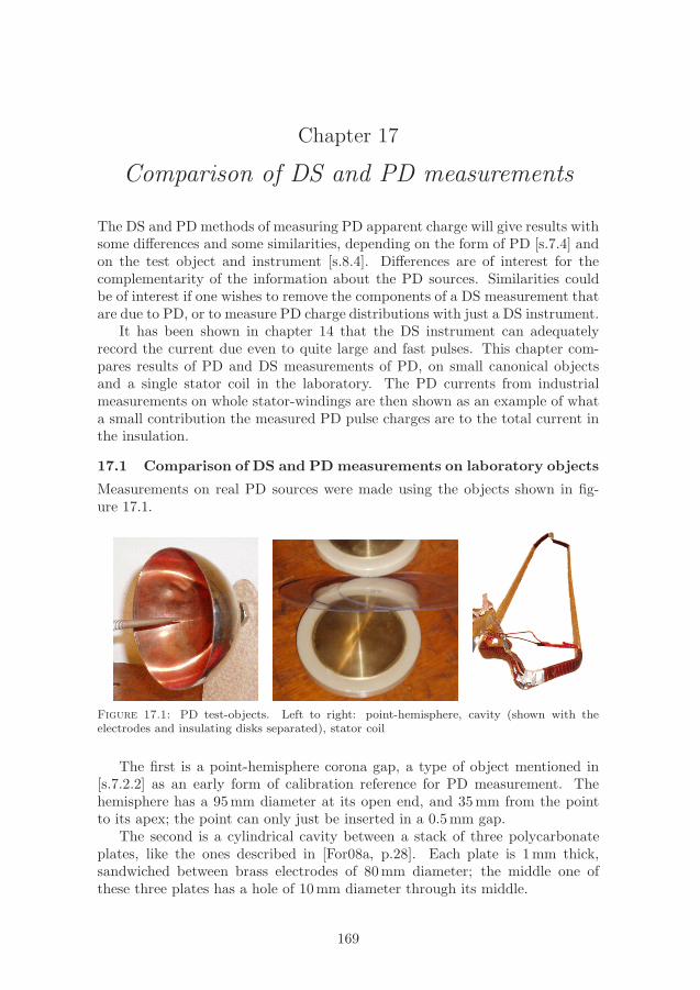
Chapter 17
Comparison of DS and PD measurements
The DS and PD methods of measuring PD apparent charge will give results withsome differences and some similarities, depending on the form of PD [s.7.4] andon the test object and instrument [s.8.4]. Differences are of interest for thecomplementarity of the information about the PD sources. Similarities couldbe of interest if one wishes to remove the components of a DS measurement thatare due to PD, or to measure PD charge distributions with just a DS instrument.
It has been shown in chapter 14 that the DS instrument can adequatelyrecord the current due even to quite large and fast pulses. This chapter com-pares results of PD and DS measurements of PD, on small canonical objectsand a single stator coil in the laboratory. The PD currents from industrialmeasurements on whole stator-windings are then shown as an example of whata small contribution the measured PD pulse charges are to the total current inthe insulation.
17.1 Comparison of DS and PD measurements on laboratory objects
Measurements on real PD sources were made using the objects shown in fig-ure 17.1.
Figure 17.1: PD test-objects. Left to right: point-hemisphere, cavity (shown with theelectrodes and insulating disks separated), stator coil
The first is a point-hemisphere corona gap, a type of object mentioned in[s.7.2.2] as an early form of calibration reference for PD measurement. Thehemisphere has a 95mm diameter at its open end, and 35mm from the pointto its apex; the point can only just be inserted in a 0.5mm gap.
The second is a cylindrical cavity between a stack of three polycarbonateplates, like the ones described in [For08a, p.28]. Each plate is 1mm thick,sandwiched between brass electrodes of 80mm diameter; the middle one ofthese three plates has a hole of 10mm diameter through its middle.
169
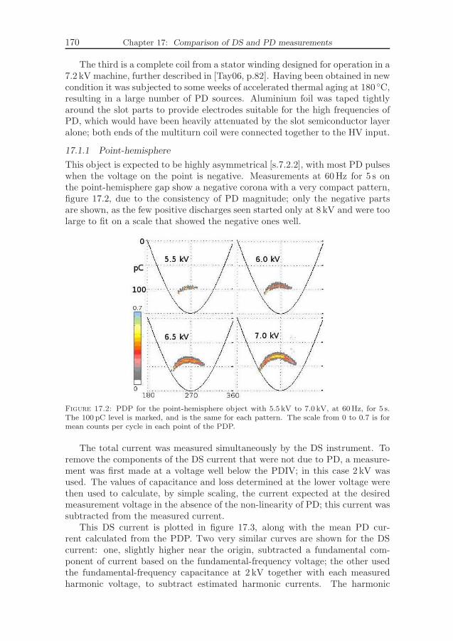
170 Chapter 17: Comparison of DS and PD measurements
The third is a complete coil from a stator winding designed for operation in a7.2 kV machine, further described in [Tay06, p.82]. Having been obtained in newcondition it was subjected to some weeks of accelerated thermal aging at 180 C,resulting in a large number of PD sources. Aluminium foil was taped tightlyaround the slot parts to provide electrodes suitable for the high frequencies ofPD, which would have been heavily attenuated by the slot semiconductor layeralone; both ends of the multiturn coil were connected together to the HV input.
17.1.1 Point-hemisphere
This object is expected to be highly asymmetrical [s.7.2.2], with most PD pulseswhen the voltage on the point is negative. Measurements at 60Hz for 5 s onthe point-hemisphere gap show a negative corona with a very compact pattern,figure 17.2, due to the consistency of PD magnitude; only the negative partsare shown, as the few positive discharges seen started only at 8 kV and were toolarge to fit on a scale that showed the negative ones well.
Figure 17.2: PDP for the point-hemisphere object with 5.5 kV to 7.0 kV, at 60Hz, for 5 s.The 100 pC level is marked, and is the same for each pattern. The scale from 0 to 0.7 is formean counts per cycle in each point of the PDP.
The total current was measured simultaneously by the DS instrument. Toremove the components of the DS current that were not due to PD, a measure-ment was first made at a voltage well below the PDIV; in this case 2 kV wasused. The values of capacitance and loss determined at the lower voltage werethen used to calculate, by simple scaling, the current expected at the desiredmeasurement voltage in the absence of the non-linearity of PD; this current wassubtracted from the measured current.
This DS current is plotted in figure 17.3, along with the mean PD cur-rent calculated from the PDP. Two very similar curves are shown for the DScurrent: one, slightly higher near the origin, subtracted a fundamental com-ponent of current based on the fundamental-frequency voltage; the other usedthe fundamental-frequency capacitance at 2 kV together with each measuredharmonic voltage, to subtract estimated harmonic currents. The harmonic

17.1.2 Cavity object 171
0 0.002 0.004 0.006 0.008 0.01 0.012 0.014 0.016 0.018−4
−3
−2
−1
0
1
2
3
4x 10
−6
time [s]
curr
ent [
A]
PD current
DS (harmonics 1−−8)
(voltage phase)
PD current(harmonics 1−−8)
Figure 17.3: Measurements of PD currents for the point-hemisphere object, using the DSand PD instruments.
voltages are clearly so low in this case that the difference is negligible: at higherloading of the supply, with a larger test-object, this might not be true [s.6.2.3].
The PD current measured by the PD system is also shown after filtering inthe frequency domain to remove components beyond the 8th harmonic; this wasdone for easier comparison of shape, as the DS system’s output is limited to thefirst 8 harmonics.
The magnitude measured by DS is almost twice as great for the negativecorona as the measurement from the PD system. How much this is due todeadtime and how much to errors in subtraction of the other currents in DSis not known. The filtered version of the PD current from the PD systemmakes clear that a strong asymmetry can be described in just eight harmonics,although with the artificial zero offset that is inevitable when omitting the dcterm as the DS instrument does. This suggests that the considerable positivecurrent, seen only in the DS measurement, is a genuine result that is missedin the pulse measurement; this is not surprising if non-pulsed drift can returnsome charges to the point when the polarity changes.
The point-hemisphere object is therefore a case with complementarity of DSand PD measurements, although the order of magnitude of currents is similar.
17.1.2 Cavity object
Measurements at 8 kV 60Hz for 120 s on the cavity object gave strongly symmet-ric positive and negative parts, so only the positive part is shown, in figure 17.4.The spread of charge magnitudes is large. In the first case (a), the ICM’sLLD threshold is at 4%, just above background noise, and the deadtime is at itsminimum 5µs: the pattern shows a strong cluster of pulses at the lowest charges,which are presumably subsequent oscillations, ‘ringing’, of the instrument’s

172 Chapter 17: Comparison of DS and PD measurements
Figure 17.4: PDPs for the cavity object. See text for details. The coloured scale is meancounts per cycle in each point of the PDP.
response, not decayed enough in the deadtime. In (b) the threshold is 10%,still with 5µs deadtime, removing the small pulses. In (c) the threshold is again4%, but with 10µs deadtime: the fact that the lower group of pulses disappearsby either the deadtime or the threshold setting indicates that the small pulseswere indeed artifacts of the instrument response.
The corresponding currents, and the measurement by DS, are shown infigure 17.5. The same methods have been used as with the point-hemisphere
0 0.002 0.004 0.006 0.008 0.01 0.012 0.014 0.016 0.018−2
−1.5
−1
−0.5
0
0.5
1
1.5
2x 10
−6
time [s]
curr
ent [
A]
PD current
PD current(harmonics 1−−8)
DS (harmonics 1−−8)
(voltage phase)
Figure 17.5: Measurements of PD currents for the cavity object
object, to subtract the non-PD components in the DS results and to plot aharmonic-limited (filtered) PD current for comparison. This gives remarkablyclose correspondence between the two measurements during the time of PD,although the filtered PD current makes it clear that poor fit around the zerosis not just an artifact of the limited harmonics in the DS results.
For this object, the DS and PD measurements therefore give similar ratherthan complementary results.

17.1.3 A single stator-coil 173
17.1.3 A single stator-coil
When making measurements on the stator coil of figure 17.1, the currents in thenonlinear stress-grading coatings in the end-windings were guarded away fromthe DS measurement, so as to include only the currents in the slot-parts of thecoil. The usual method of estimating and subtracting the currents due to theobject’s capacitance was thereby made possible without resort to the vaguenessof stress-grading models.
It should be noted that these results were made earlier [Tay06], with olderinstruments, and not simultaneously. It was however checked that PD behaviourwas quite consistent between measurements, so that differences even of a factorof two would be very surprising.
Figure 17.6 compares the currents measured by the PD pulse and DS meth-ods. In contrast to the two simple objects, the current from the PD pulse
0 45 90 135 180 225 270 315 360−1.5
−1
−0.5
0
0.5
1
1.5x 10
−4
Phase, degrees
Cur
rent
, A
harmonics 1−8 of PD signal, scaled to match DS
DS current after removal of LV capacitance
PD current, rawand filtered
(harmonics 1−8)
Figure 17.6: Stator-coil PD current from DS and PD systems
measurement has had to be scaled up by several times, to match the DSmeasurement.
Measurements at other frequencies are shown in figure 17.7. Large anddifferent factors, marked on the graphs, were needed to make the amplitudesmatch. The waveforms all match well, but the amplitudes vary by up to50 times, with the DS system measuring the larger currents. Note that ifthe estimated non-PD current subtracted from the DS system were severelywrong, so that this could be the main cause of the difference between the twomeasurements, then the resulting PD current would have a much more sinusoidalshape, since the subtracted component is practically sinusoidal.
These results strongly indicate that the PD pulse-measurement instrumentis missing a lot of charge with this object, but the DS system is measuring it.This is no surprise, as even the single coil had a severe degree of aging and many,easily audible, PD sources. The necessary dead-time was 50µs in this case, toavoid ringing from the relatively large object, so frequent PD from many sources
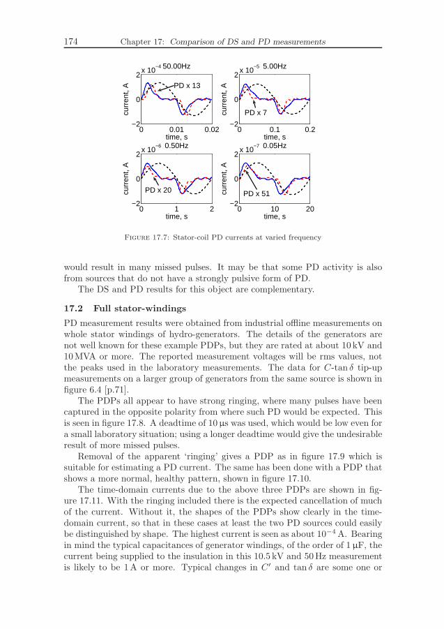
174 Chapter 17: Comparison of DS and PD measurements
0 0.01 0.02−2
0
2x 10
−4
time, s
curr
ent,
A
50.00Hz
0 0.1 0.2−2
0
2x 10
−5
time, s
curr
ent,
A
5.00Hz
0 1 2−2
0
2x 10
−6
time, s
curr
ent,
A
0.50Hz
0 10 20−2
0
2x 10
−7
time, scu
rren
t, A
0.05Hz
PD x 13
PD x 7
PD x 20 PD x 51
Figure 17.7: Stator-coil PD currents at varied frequency
would result in many missed pulses. It may be that some PD activity is alsofrom sources that do not have a strongly pulsive form of PD.
The DS and PD results for this object are complementary.
17.2 Full stator-windings
PD measurement results were obtained from industrial offline measurements onwhole stator windings of hydro-generators. The details of the generators arenot well known for these example PDPs, but they are rated at about 10 kV and10MVA or more. The reported measurement voltages will be rms values, notthe peaks used in the laboratory measurements. The data for C-tan δ tip-upmeasurements on a larger group of generators from the same source is shown infigure 6.4 [p.71].
The PDPs all appear to have strong ringing, where many pulses have beencaptured in the opposite polarity from where such PD would be expected. Thisis seen in figure 17.8. A deadtime of 10µs was used, which would be low even fora small laboratory situation; using a longer deadtime would give the undesirableresult of more missed pulses.
Removal of the apparent ‘ringing’ gives a PDP as in figure 17.9 which issuitable for estimating a PD current. The same has been done with a PDP thatshows a more normal, healthy pattern, shown in figure 17.10.
The time-domain currents due to the above three PDPs are shown in fig-ure 17.11. With the ringing included there is the expected cancellation of muchof the current. Without it, the shapes of the PDPs show clearly in the time-domain current, so that in these cases at least the two PD sources could easilybe distinguished by shape. The highest current is seen as about 10−4 A. Bearingin mind the typical capacitances of generator windings, of the order of 1 µF, thecurrent being supplied to the insulation in this 10.5 kV and 50Hz measurementis likely to be 1A or more. Typical changes in C′ and tan δ are some one or
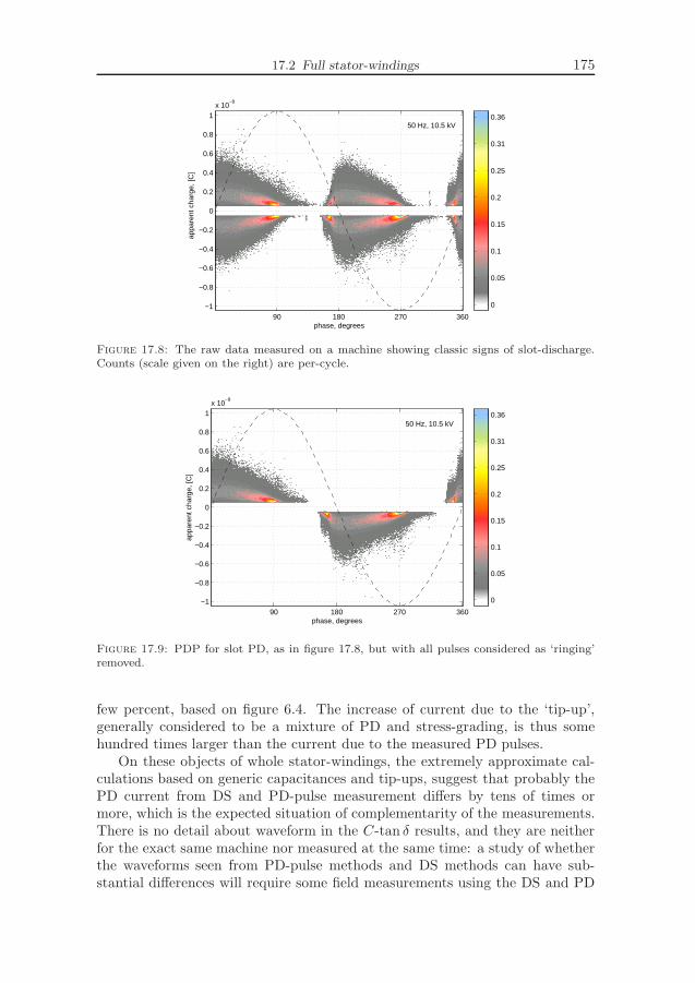
17.2 Full stator-windings 175
phase, degrees
appa
rent
cha
rge,
[C]
50 Hz, 10.5 kV
90 180 270 360−1
−0.8
−0.6
−0.4
−0.2
0
0.2
0.4
0.6
0.8
1x 10
−8
0
0.05
0.1
0.15
0.2
0.25
0.31
0.36
Figure 17.8: The raw data measured on a machine showing classic signs of slot-discharge.Counts (scale given on the right) are per-cycle.
phase, degrees
appa
rent
cha
rge,
[C]
50 Hz, 10.5 kV
90 180 270 360−1
−0.8
−0.6
−0.4
−0.2
0
0.2
0.4
0.6
0.8
1x 10
−8
0
0.05
0.1
0.15
0.2
0.25
0.31
0.36
Figure 17.9: PDP for slot PD, as in figure 17.8, but with all pulses considered as ‘ringing’removed.
few percent, based on figure 6.4. The increase of current due to the ‘tip-up’,generally considered to be a mixture of PD and stress-grading, is thus somehundred times larger than the current due to the measured PD pulses.
On these objects of whole stator-windings, the extremely approximate cal-culations based on generic capacitances and tip-ups, suggest that probably thePD current from DS and PD-pulse measurement differs by tens of times ormore, which is the expected situation of complementarity of the measurements.There is no detail about waveform in the C-tan δ results, and they are neitherfor the exact same machine nor measured at the same time: a study of whetherthe waveforms seen from PD-pulse methods and DS methods can have sub-stantial differences will require some field measurements using the DS and PD

176 Chapter 17: Comparison of DS and PD measurements
phase, degrees
appa
rent
cha
rge,
[C]
50 Hz, 10.5 kV
90 180 270 360−1
−0.8
−0.6
−0.4
−0.2
0
0.2
0.4
0.6
0.8
1x 10
−8
0
0.05
0.1
0.15
0.2
0.25
0.31
0.36
Figure 17.10: PDP for a ‘normal’ stator winding. As with figure 17.9, this has had quitesimilar clusters of pulses with opposite signs removed.
0 45 90 135 180 225 270 315 360
−8
−6
−4
−2
0
2
4
6
8
x 10−5
phase, degrees (’normalised time’)
curr
ent,
[A]
slot
’normal’
slot, includingprobable ’ringing’
Figure 17.11: Mean currents due to the PDPs in figures 17.10 (normal), 17.9 (slot-PD), and17.8 (slot-PD, including ’ringing’).
instruments together.

Chapter 18
Stator coils used as test-objects
Several newly manufactured multiturn coils were obtained for measurements ofmaterial properties, end-grading currents and thermal aging. Three of themwere used for measurements reported in this work. This chapter describes thecoils and the oven made for heating them, and presents results from dielectricmeasurements made on the main insulation. Material properties of the end-winding stress-grading are presented in chapter 20, and the contribution ofthe end-windings to the total dielectric response is presented in chapter 19.Measurements of DS and PD on an earlier batch of coils after strong thermalaging have been described already in [Tay06].
18.1 Construction
Three coils were manufactured to the same specification, in the same batch.After VPI and curing, each of the three coils was sawn through at its extremeends, to make two coil-halves (hereafter called bars) for easier handling andseparate testing. The six bars are shown in figure 18.1.
Figure 18.1: Left: all six stator-bars, showing half the slot-section and part of the end; inthe background are the two bars without metal plates, for material measurements. Right:end-view showing strands before (top) and after (bottom) connecting with conductive paint.
The conductors in the coils were 6 turns of 4 parallel copper conductors(strands), in two stacks; the bars therefore have two stacks of 12 separatestrands. For measurements the strands were all connected together at bothends. A copper wire was stretched across between the stacks, and a silver-basedconductive paint was used to connect all the surfaces to each other and to thewire; soldering even with a blowlamp was infeasible because of the high thermalconductivity of the copper.
177
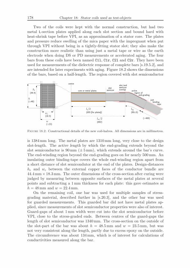
178 Chapter 18: Stator coils used as test-objects
Two of the coils were kept with the normal construction, but had twometal L-section plates applied along each slot section and bound hard withheat-shrink tape before VPI, as an approximation of a stator core. The platesand pressure reduce swelling of the mica paper with the impregnant when putthrough VPI without being in a tightly-fitting stator slot; they also make theconstruction more realistic than using just a metal tape or wire as the earthelectrode when doing DS or PD measurements or accelerated aging. The fourbars from these coils have been named C1l, C1r, C2l and C2r. They have beenused for measurements of the dielectric response of complete bars [s.19.5.2], andare intended for later experiments with aging. Figure 18.2 shows the dimensionsof the bars, based on a half-length. The region covered with slot semiconductor
centre
lsg
active
just
overlapsemiconslot/end
h
w
wc
semiconslot
(90±5)
(>400)(18.3)
(≃48)
(≃23)
(44.4)core or metal plateshc
region ofend-grading
bindingtape
ls/2(655 [for plates])
lsc/2(692)
Figure 18.2: Constructional details of the new coil-halves. All dimensions are in millimetres.
is 1384mm long. The metal plates are 1310mm long, very close to the designslot-length. The active length by which the end-grading extends beyond theslot semiconductor is 90mm (± 5mm), which extends around the bar’s curve.The end-winding region beyond the end-grading goes on for nearly 500mm. Aninsulating outer binding-tape covers the whole end-winding region apart froma short distance of slot semicondutor at the end of the plates. Design-distanceshc and wc between the external copper faces of the conductor bundle are44.4mm× 18.3mm. The outer dimensions of the cross-section after curing werejudged by measuring between opposite surfaces of the metal plates at severalpoints and subtracting a 1mm thickness for each plate: this gave estimates ash = 48mm and w = 22.4mm.
On the remaining coil, one bar was used for multiple samples of stress-grading material, described further in [s.20.3], and the other bar was usedfor guarded measurements. This guarded bar did not have metal plates ap-plied, since measurements of slot semiconductor properties were also of interest.Guard-gaps of about 1mm width were cut into the slot semiconductor beforeVPI, close to the stress-graded ends. Between centres of the guard-gaps thelength of slot semiconductor was 1340mm. The cross-section on the outside ofthe slot-part of the bar was about h = 48.5mm and w = 23.5mm, but wasnot very consistent along the length, partly due to excess epoxy on the outside.The circumference was about 134mm, which is of interest for calculations ofconductivities measured along the bar.

18.2 Heating 179
18.2 Heating
Earlier work in this project used severe thermal aging to change pristine sta-tor coils into intensely PD-infested test-objects, as reported in [Tay06]. Thisinvolved time-consuming transportation to and from a borrowed oven of largeenough size in another town. It was hard to make progressive measurementsduring aging, and was clearly not a reasonable long-term approach. A largeoven was instead built in the laboratory, to permit versatile work with aging.
An aluminium box of 2.5m × 1.25m × 0.75m was built, and was insulatedon all faces with rockwool of 45mm thickness, surrounded by an outer layerof aluminium foil to reduce air movement and radiative loss. The outside andinside are shown in figure 18.3. Four hot-plates from the top of a domestic
Figure 18.3: The large laboratory-oven for thermal aging. On the left, with and without thelid and its insulation. On the right, four normal bars and two material-sample bars are inplace, and heater elements are visible at the right.
cooker were used as heaters; they were placed along the base of the box at oneside, connected with wires insulated with silicone-rubber. Wire-mesh basketswere placed along the other side as shelves for the test-objects, which thus restedat about half the height of the box, at the other side from the heaters.
The heaters each had three available resistances; connections were chosento give two groups, of powers 1.6kW and 2.1 kW, with the four heaters con-tributing quite similarly to each. The 1.6 kW group alone gave an equilibriumtemperature of about 160 C. Warm-up from room temperature to 180 C tookjust under an hour with both groups together. A domestic oven-thermostat wasused for temperature-control. Depending on the required temperature, either
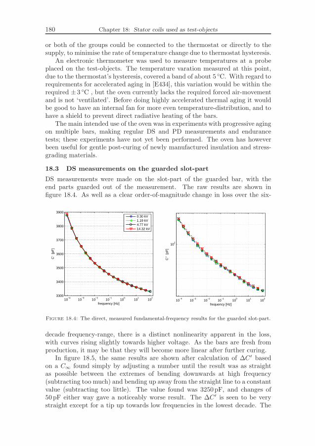
180 Chapter 18: Stator coils used as test-objects
or both of the groups could be connected to the thermostat or directly to thesupply, to minimise the rate of temperature change due to thermostat hysteresis.
An electronic thermometer was used to measure temperatures at a probeplaced on the test-objects. The temperature varation measured at this point,due to the thermostat’s hysteresis, covered a band of about 5 C. With regard torequirements for accelerated aging in [E434], this variation would be within therequired ± 3 C , but the oven currently lacks the required forced air-movementand is not ‘ventilated’. Before doing highly accelerated thermal aging it wouldbe good to have an internal fan for more even temperature-distribution, and tohave a shield to prevent direct radiative heating of the bars.
The main intended use of the oven was in experiments with progressive agingon multiple bars, making regular DS and PD measurements and endurancetests; these experiments have not yet been performed. The oven has howeverbeen useful for gentle post-curing of newly manufactured insulation and stress-grading materials.
18.3 DS measurements on the guarded slot-part
DS measurements were made on the slot-part of the guarded bar, with theend parts guarded out of the measurement. The raw results are shown infigure 18.4. As well as a clear order-of-magnitude change in loss over the six-
10−4
10−3
10−2
10−1
100
101
102
3300
3400
3500
3600
3700
3800
3900
frequency [Hz]
C’
[pF
]
10−4
10−3
10−2
10−1
100
101
102
102
frequency [Hz]
C’’
[pF
]
0.30 kV1.19 kV4.77 kV14.32 kV
Figure 18.4: The direct, measured fundamental-frequency results for the guarded slot-part.
decade frequency-range, there is a distinct nonlinearity apparent in the loss,with curves rising slightly towards higher voltage. As the bars are fresh fromproduction, it may be that they will become more linear after further curing.
In figure 18.5, the same results are shown after calculation of ∆C′ basedon a C∞ found simply by adjusting a number until the result was as straightas possible between the extremes of bending downwards at high frequency(subtracting too much) and bending up away from the straight line to a constantvalue (subtracting too little). The value found was 3250pF, and changes of50 pF either way gave a noticeably worse result. The ∆C′ is seen to be verystraight except for a tip up towards low frequencies in the lowest decade. The
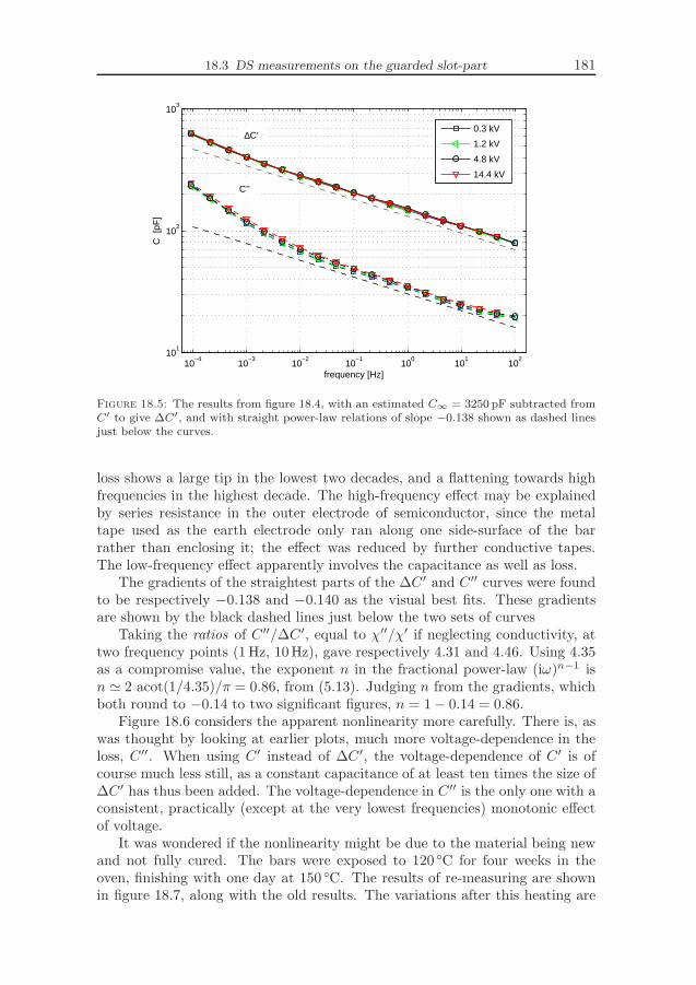
18.3 DS measurements on the guarded slot-part 181
10−4
10−3
10−2
10−1
100
101
102
101
102
103
frequency [Hz]
C [
pF]
0.3 kV
1.2 kV
4.8 kV
14.4 kV
∆C’
C’’
Figure 18.5: The results from figure 18.4, with an estimated C∞ = 3250 pF subtracted fromC′ to give ∆C′, and with straight power-law relations of slope −0.138 shown as dashed linesjust below the curves.
loss shows a large tip in the lowest two decades, and a flattening towards highfrequencies in the highest decade. The high-frequency effect may be explainedby series resistance in the outer electrode of semiconductor, since the metaltape used as the earth electrode only ran along one side-surface of the barrather than enclosing it; the effect was reduced by further conductive tapes.The low-frequency effect apparently involves the capacitance as well as loss.
The gradients of the straightest parts of the ∆C′ and C′′ curves were foundto be respectively −0.138 and −0.140 as the visual best fits. These gradientsare shown by the black dashed lines just below the two sets of curves
Taking the ratios of C′′/∆C′, equal to χ′′/χ′ if neglecting conductivity, attwo frequency points (1 Hz, 10Hz), gave respectively 4.31 and 4.46. Using 4.35as a compromise value, the exponent n in the fractional power-law (iω)n−1 isn ≃ 2 acot(1/4.35)/π = 0.86, from (5.13). Judging n from the gradients, whichboth round to −0.14 to two significant figures, n = 1 − 0.14 = 0.86.
Figure 18.6 considers the apparent nonlinearity more carefully. There is, aswas thought by looking at earlier plots, much more voltage-dependence in theloss, C′′. When using C′ instead of ∆C′, the voltage-dependence of C′ is ofcourse much less still, as a constant capacitance of at least ten times the size of∆C′ has thus been added. The voltage-dependence in C′′ is the only one with aconsistent, practically (except at the very lowest frequencies) monotonic effectof voltage.
It was wondered if the nonlinearity might be due to the material being newand not fully cured. The bars were exposed to 120 C for four weeks in theoven, finishing with one day at 150 C. The results of re-measuring are shownin figure 18.7, along with the old results. The variations after this heating are

182 Chapter 18: Stator coils used as test-objects
10−4
10−3
10−2
10−1
100
101
102
0.98
0.99
1
1.01
1.02
frequency [Hz]
mea
sure
d ∆C
’ rel
ativ
e to
14.
4kV
10−4
10−3
10−2
10−1
100
101
102
0.92
0.94
0.96
0.98
1
frequency [Hz]
mea
sure
d C
’’ re
lativ
e to
14.
4kV
0.3 kV
1.2 kV
4.8 kV
14.4 kV
Figure 18.6: For ∆C′ and C′′, the ratios of the curves at all four voltages to the valuesobtained at the highest voltage.
10−4
10−3
10−2
10−1
100
101
3400
3500
3600
3700
3800
3900
frequency [Hz]
C’
[pF
]
0.30 kV
1.19 kV
4.77 kV
14.32 kV
10−4
10−3
10−2
10−1
100
101
102
102
frequency [Hz]
C’’
[pF
]
Figure 18.7: Capacitance and loss for the guarded slot part, before (x) and after (o)‘postcuring’ at about 120 C for four weeks.
even somewhat larger, although not so consistent. A measurement on a 100 pFgas capacitor using the same connections showed no clear trend with voltage,so it does seem likely that the bar is the main source of nonlinearity. Comparedto the effect of the stress-graded end-windings, this is very small variation withvoltage, but it is interesting to know that the linearity might be a problem ifwanting to make sensitive measurements of PD current by DS methods.
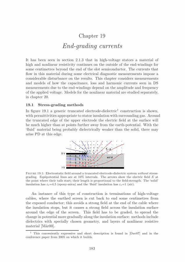
Chapter 19
End-grading currents
It has been seen in section 2.1.3 that in high-voltage stators a material ofhigh and nonlinear resistivity continues on the outside of the end-windings forsome centimetres beyond the end of the slot semiconductor. The currents thatflow in this material during some electrical diagnostic measurements impose aconsiderable disturbance on the results. This chapter considers measurementsand models of how the capacitance, loss and harmonic currents seen in DSmeasurements due to the end-windings depend on the amplitude and frequencyof the applied voltage. Models for the nonlinear material are studied separately,in chapter 20.
19.1 Stress-grading methods
In figure 19.1 a generic truncated electrode-dielectric† construction is shown,with permittivities appropriate to stator insulation with surrounding gas. Aroundthe truncated edge of the upper electrode the electric field at the surface willbe much higher than at points further away from the earth-potential. With the‘fluid’ material being probably dielectrically weaker than the solid, there mayarise PD at this edge.
Figure 19.1: Electrostatic field around a truncated electrode-dielectric system without stress-grading. Equipotential lines are at 10% intervals. The arrows show the electric field E atthe point where their tails start; their length is proportional to the field-strength. The ‘solid’insulation has εr=4.5 (epoxy-mica) and the ‘fluid’ insulation has εr=1 (air).
An instance of this type of construction is terminations of high-voltagecables, where the earthed screen is cut back to end some centimetres fromthe exposed conductor; this avoids a strong field at the end of the cable wherethe insulation stops, but it causes a strong field across the insulation surfacearound the edge of the screen. This field has to be graded, to spread thechange in potential more gradually along the insulation surface: methods includedielectrics with specially chosen geometry, and layers of nonlinear resistivematerial [Mar00].
† This conveniently expressive and short description is found in [Dav07] and in theconference paper from 2005 on which it builds.
183

184 Chapter 19: End-grading currents
In stator windings the insulation of the end-winding region is particularlysensitive; there are hand-made joints made between the ends of coils or bars andpossibly their cooling pipes too, and there is a consequent difficulty of avoidingsubstantial voids where tapes have not fully come together and impregnant hasnot totally filled the space. From [Sto04, p.26], “Decades of experience showsthat even a fully insulated connection between adjacent coils will be a weak spotthat may prompt a future insulation failure if a ground potential is nearby”. Theearthed slot-semiconductor therefore ends a short distance beyond the core, toallow the outer surfaces of the end-windings to be at floating potential.
For machines rated above some 5 kV the surface electric-field could causePD, particularly in machines operating only at atmospheric pressure. Space isparticularly scarce in stator insulation, so external geometric grading of the fieldis not practicable. Some early machines used floating conductive layers within
the insulation [Sto04, p.26], as is common in bushings; there is renewed interest[Sha08] in such methods to cope with high-frequencies in motors used in IFDs[s.7.3.1]. However, most machines currently in operation beyond about 5 kV usea thin layer of nonlinearly resistive material around the bar’s surface for somecentimetres beyond the end of the slot-semiconductor; some 5 cm to 10 cm iscommon [Sto04, p.26].
19.2 Cylindrical laboratory-models on PTFE
Simple gradings were made in the laboratory to study as purely as possible theeffects of the grading material and geometry. A PTFE (polytetrafluoroethylene)tube was fitted tightly around a longer metal pipe, and an outer electrode ofcopper tape was applied for a short distance along the middle of the tube’slength. The surface of the tube beyond the outer electrode was coated with oneof two types of commercial stress-grading material for stator end-windings, apaint or a tape. A cross-section is shown in figure 19.2.
40mm 20mm40mm
80mm 60mm40mm
50mm
grading
5.5mm
10mm
axis ofreflection
symmetry
axis of rotation−symmetry
earthed sheath
(tape)(paint)
(tape)(paint)
PTFE
metal tube
Figure 19.2: A quarter cross-section of the simple physical models.
The cylindrical shape was chosen for convenience of assembly and for easyanalysis. The PTFE insulation was chosen for ease of handling, tolerance of therequired two hours at 160C for curing resin-based grading tapes, and for itslow dispersion in our frequency range such that it can reasonably be regardedas having a fixed permittivity. The two-ended construction was used to preventPD or leakage that could occur if one end were left open. The middle section
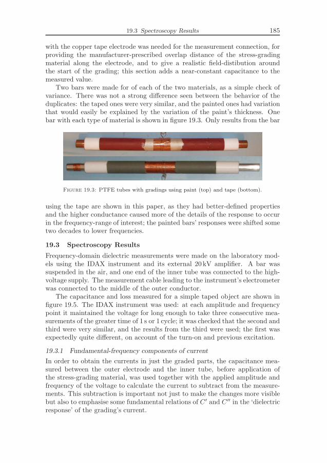
19.3 Spectroscopy Results 185
with the copper tape electrode was needed for the measurement connection, forproviding the manufacturer-prescribed overlap distance of the stress-gradingmaterial along the electrode, and to give a realistic field-distibution aroundthe start of the grading; this section adds a near-constant capacitance to themeasured value.
Two bars were made for of each of the two materials, as a simple check ofvariance. There was not a strong difference seen between the behavior of theduplicates: the taped ones were very similar, and the painted ones had variationthat would easily be explained by the variation of the paint’s thickness. Onebar with each type of material is shown in figure 19.3. Only results from the bar
Figure 19.3: PTFE tubes with gradings using paint (top) and tape (bottom).
using the tape are shown in this paper, as they had better-defined propertiesand the higher conductance caused more of the details of the response to occurin the frequency-range of interest; the painted bars’ responses were shifted sometwo decades to lower frequencies.
19.3 Spectroscopy Results
Frequency-domain dielectric measurements were made on the laboratory mod-els using the IDAX instrument and its external 20 kV amplifier. A bar wassuspended in the air, and one end of the inner tube was connected to the high-voltage supply. The measurement cable leading to the instrument’s electrometerwas connected to the middle of the outer conductor.
The capacitance and loss measured for a simple taped object are shown infigure 19.5. The IDAX instrument was used: at each amplitude and frequencypoint it maintained the voltage for long enough to take three consecutive mea-surements of the greater time of 1 s or 1 cycle; it was checked that the second andthird were very similar, and the results from the third were used; the first wasexpectedly quite different, on account of the turn-on and previous excitation.
19.3.1 Fundamental-frequency components of current
In order to obtain the currents in just the graded parts, the capacitance mea-sured between the outer electrode and the inner tube, before application ofthe stress-grading material, was used together with the applied amplitude andfrequency of the voltage to calculate the current to subtract from the measure-ments. This subtraction is important not just to make the changes more visiblebut also to emphasise some fundamental relations of C′ and C′′ in the ‘dielectricresponse’ of the grading’s current.

186 Chapter 19: End-grading currents
10−4
10−3
10−2
10−1
100
101
102
10−12
10−11
frequency, Hz
Cp,
Cb
(C
’,C’’,
Far
ads)
987.81 Vpk
2.97 kVpk
4.95 kVpk
6.92 kVpk
8.90 kVpk
10.88 kVpk
12.86 kVpk
increasingvoltage
C’’
C’
Figure 19.4: Fundamental-frequency components measured for bar5 (taped).
Several distinctive features can be seen. Towards low frequencies the ca-pacitance tends to a constant irrespective of the amplitude of the voltage. Thisconstant value is the capacitance of the PTFE insulation along the full length ofthe gradings: at low enough frequency the zero-potential from the electrode atthe start of the grading has spread all along the grading, because the impedanceof the capacitive insulation is so high at the low frequency.
The loss curves have peaks that are shifted up in frequency and very slightlydown in value, with increased voltage. A primitive description of the gradingas a series RC circuit with a resistance that decreases with increased voltage,suggests that this shift to higher frequencies, i.e. to lower time-constants RC,with increased voltage is reasonable. At frequencies above the loss peak thecapacitance and loss tend to straight lines: for the lower voltages these linesare not only parallel but are indeed superposed. More attention is given to thislater, when discussing models.
19.3.2 Harmonic currents
When the measured object is significantly nonlinear, as is the case here, thefundamental-frequency components of current in response to the sinusoidalapplied voltage are only a part of the object’s description. The harmonics in thecurrent give an idea of the nonlinearity. Even-order harmonics are not expected,as the object has symmetric properties with respect to polarity: the magnitudesof the all even harmonics in current were well below the 7th harmonic shownhere. The third harmonic reaches 15% of the fundamental, and its relativevalue has much more dependence on the frequency than on the amplitude ofthe applied voltage over the reasonable dynamic range of these two parameters.

19.4 Numerical Models 187
19.4 Numerical Models
Some previous users of a (1D) ‘transmission-line’ model are listed for applica-tions to cable terminations, in references 5 – 10 of [Lup96] and to stator end-windings in references 38 – 41 of [Dav07].
Other forms of model include an assumption of i(t) ∝ t−1/2 for the end-grading current in time-domain spectroscopy [Gof00], and a model based on a‘perfect’ sharp nonlinearity such that the material is insulating below a certainfield, then prevents any further rise of the field [Kel67], developed further intoexpressions for FDDS results in [Pin98].
The numerical model that is used at the end of this section is based on aone-dimensional distribution of parallel fixed capacitance and nonlinear seriesresistance using the material properties described in chapter 20. This type ofmodel has been used in other work cited in the previous section, in studies ofstress-distribution and heating at high frequencies. On the way to this model,several steps of detail are used, explaining the causes of the features notedabout the experimental results for C′ and C′′ as functions of voltage amplitudeand frequency. The models consider a single grading, one end of the tubularlaboratory-model.
The basic features of the results from the four levels of model are shown infigure 19.5. The models are explained, and their results studied, in the followingsubsections.
19.4.1 Linear, discrete
A very simple model of the grading is a single discrete resistance and capacitancein series. The current into this arrangement, seen in the usual form of capac-itance and loss, gives the classic Debye response. As the model is linear thereis no voltage-dependence of the curves. As a simple first step to modeling thenonlinearity, the resistance is varied instead, depending on the applied voltageamplitude. Only the ‘tape’ grading material is used, as it had so much moreconsistent properties than the paint.
As an example a capacitance of 21.3 pF was used, which is the total ca-pacitance of the PTFE tube under the 80mm length of the grading, excludingfringing. A resistance of 145GΩ was chosen, which is the zero-field resistanceof the 80mm grading length.
Towards high frequencies the slopes are much too steep, compared to theexperimental results, being Debye slopes where C′ and C′′ fall off at slopes −2and −1 ‘decades per decade’. The experimental results had both slopes around−0.5 at low voltages, and at higher voltage they were even shallower. Towardslow frequencies the electric field in the grading is so low that the conductivityis near its zero-field value and is not much dependent on the applied voltage.The experimental results show this in that the loss curves at different voltagesconverging towards low frequency; the fixed resistance used here for each appliedvoltage cannot show this effect.
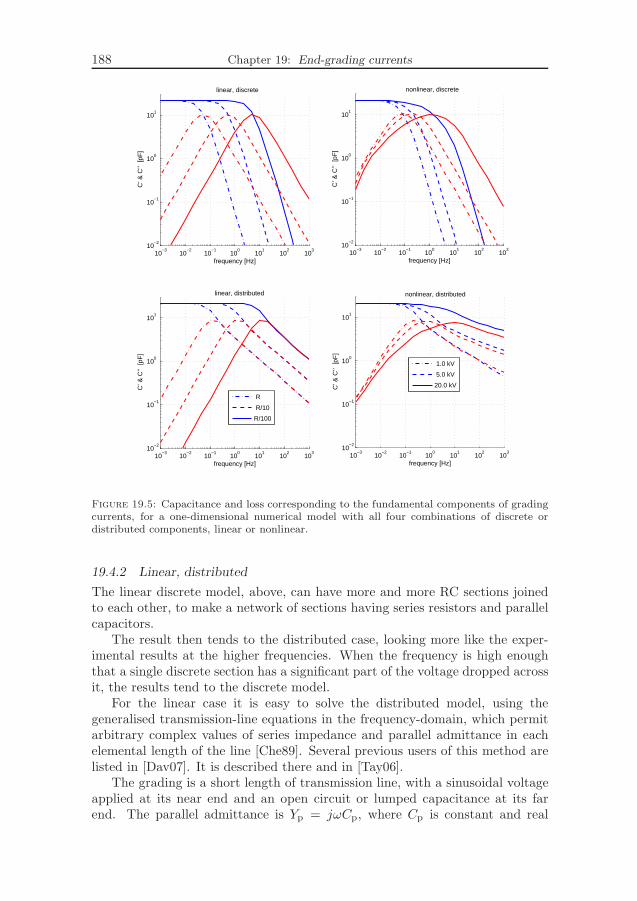
188 Chapter 19: End-grading currents
10−3
10−2
10−1
100
101
102
103
10−2
10−1
100
101
frequency [Hz]
C’ &
C’’
[pF
]
linear, discrete
10−3
10−2
10−1
100
101
102
103
10−2
10−1
100
101
frequency [Hz]
C’ &
C’’
[pF
]
nonlinear, discrete
10−3
10−2
10−1
100
101
102
103
10−2
10−1
100
101
frequency [Hz]
C’ &
C’’
[pF
]
linear, distributed
R
R/10
R/100
10−3
10−2
10−1
100
101
102
103
10−2
10−1
100
101
frequency [Hz]
C’ &
C’’
[pF
]
nonlinear, distributed
1.0 kV
5.0 kV
20.0 kV
Figure 19.5: Capacitance and loss corresponding to the fundamental components of gradingcurrents, for a one-dimensional numerical model with all four combinations of discrete ordistributed components, linear or nonlinear.
19.4.2 Linear, distributed
The linear discrete model, above, can have more and more RC sections joinedto each other, to make a network of sections having series resistors and parallelcapacitors.
The result then tends to the distributed case, looking more like the exper-imental results at the higher frequencies. When the frequency is high enoughthat a single discrete section has a significant part of the voltage dropped acrossit, the results tend to the discrete model.
For the linear case it is easy to solve the distributed model, using thegeneralised transmission-line equations in the frequency-domain, which permitarbitrary complex values of series impedance and parallel admittance in eachelemental length of the line [Che89]. Several previous users of this method arelisted in [Dav07]. It is described there and in [Tay06].
The grading is a short length of transmission line, with a sinusoidal voltageapplied at its near end and an open circuit or lumped capacitance at its farend. The parallel admittance is Yp = jωCp, where Cp is constant and real
19.4.2 Linear, distributed 189
to a good approximation for PTFE. The series impedance Zs = R, to whichone may wish to add a parallel capacitive component for the higher frequencieswhere the conductivity of the grading material is not dominant over the effectivepermittivity in the grading material and the parallel air and solid insulation.The situation thus described is diffusion rather than the wave-propagationthat occurs when there is significant series inductance. with typical gradingparameters the speed at which the applied voltage travels along the grading isvery slow, as is seen from the experimental results that show the low frequencies,and therefore the long periods, which the applied voltage must have before theend of the grading becomes significant and causes C′ to stop rising.
The desired output value from the model is the current into the distributednetwork. The closest standard transmission line value [Che89] to the inputcurrent or the complex capacitance is the input impedance Zin,
Zin = Z0Zend + Z0 tanh(γl)
Z0 + Zend tanh(γl)(19.1)
where l is the length of the line (grading), Zend is the impedance terminatingthe far end, and the characteristic-impedance Z0 and propagation constant γare given by
Z0 =
√
Zs
Yp=
√
R
iωC
γ =√
ZsYp =√
iωCR
in which R and C, and therefore Zs, Yp and γ, are all values per unit length.In a simple open-ended model (19.1) needs to be cancelled to
Zin =Z0
tanh(γl)(when Zend = ∞) (19.2)
Any function of frequency can be used in Zs and Yp. For example, C may be acomplex capacitance, or a capacitance may be included in parallel with R. Thesimple RC case is treated here, since it extends the linear discrete model in justone way. The complex capacitance is found as
C′ − iC′′ =1
iωZin, (19.3)
which for the open-ended case is
C′ − iC′′ =
√
C
iωRtanh
(
l√
iωCR)
. (19.4)
The results from this model are shown using the same R and C values as forthe linear discrete case, distributed over the 80mm length of the grading.
There is much better fit to the experimental results around the high-frequencyparts. The reason for the slope of −0.5 is clear from (19.4), where the tanh

190 Chapter 19: End-grading currents
term tends to a real value of 1 as its argument grows, and the other termincludes 1/
√ω to give the slope, and 1/
√i to split this equally between real and
imaginary parts. This special case of the ‘universal law’, with n = 0.5, is truefor any infinite network of constant series resistance and parallel capacitance,regardless of the values R and C [Jon83, p.80].
For the finite length of our practical case, the infinite network is a goodapproximation as long as the potential from the input end doesn’t significantlychange the potential at the far end. In the low-voltage experimental resultsthis is true down to about 1Hz, but then the end of the grading starts to bereached by the diffusion within each period of the applied voltage, and theresults become similar to the linear discrete case, deviating considerably fromthose in the measurements. The linear discrete and distributed cases differ fromeach other too at the low frequencies, as the effective resistance is higher in thediscrete case where the total capacitance was lumped at the end of the totalresistance. This could be improved by scaling the resistance, but these simplestmodels were only intended to give qualitative comparions.
At high voltages the material behaves sufficiently nonlinearly that it doesnot so strongly show the power-law n = 0.5 response: the values of C′ areshifted higher than C′′, and the gradient is less steep, both of these featurescorresponding to n > 0.5. The grading no longer can be modelled as having itsparameter R constant along its length.
19.4.3 Nonlinear, discrete
The effect of nonlinearity, but without the distributed RC nature, can be seenby replacing the discrete resistor with a conductance with voltage-dependencefollowing the material conductivity equation such as (20.3). The total capaci-tance and total zero-field series resistance of the 80mm grading were used, asin the linear discrete model.
With a sinusoidal applied voltage vin across the series-connected capacitanceC and nonlinear resistance of zero-voltage resistance R, the voltage vc acrossthe capacitor is the state-variable in an ODE,
Cdvc
dt= (vin−vc)
1
Rexp
(
n |vin−vc|2/3)
. (19.5)
This was solved numerically, using the ode45 ODE solver in Matlab 7.5. Thecurrent into the grading is provided by the same solution, as it is the right-handside of (19.5). The initial condition was vc = 0; the calculation was run for fourcycles to reach an equilibrium, then 32 values of current at evenly spaced timeswere taken from each of the next two cycles. An FFT was performed to obtainthe capacitance and loss as well as the low harmonics. The whole calculationwas repeated over a range of amplitudes and frequencies of vin.
Towards higher frequencies the excessively steep gradients are seen, as in thelinear discrete model. The heights of the loss-peaks do show a slight increaseat lower voltages, as in the experimental results. The main improvement thathas happened here, compared to the linear discrete model, is the convergenceof the values of C′′ towards low frequency; the nonlinear model has less voltageacross the nonlinear resistance when at lower frequencies.

19.4.4 Nonlinear, distributed 191
19.4.4 Nonlinear, distributed
The final level of one-dimensional model combines the properties of nonlinearityand distributed parameters.
As well as Rs and Cp, which have been used in the previous models, thereare optional components that represent permittivity of the grading and itssurrounding in Cs, loss in the insulation in Gp, and discrete components atthe end to allow for fringing of the field or conductivity there. The possiblecomponents are shown in figure 19.6, in a general form for discrete or continuousmodels.
l / n l / n l / n
Cs Cs / d
Gend Cend
Cp d Gp dv(t)
upper values: lumped (discrete) parameterslower values: distributed parameters
total length l
ndx
Rs Rs dx
xn / l
xCp Gp
x
Figure 19.6: Components of 1D grading model
Variations on all of these components, including nonlinearities in the lumpedconductance at the end, have been tried, along with variations in the materialmodel’s parameters. No single change had a large benefit to the fit to themeasured results without also worsening the fit in other parts of the range offrequencies. The simple model using just directly measured dimensions, andmaterial properties measured on samples on PTFE tubes [s.20.2] has thereforebeen taken here, rather than arbitrarily adjusting the many possible parametersfor a better fit of the measured results.
An analytical solution for the desired frequency-domain currents is not fea-sible with the nonlinearity and the possible extra components such as Cs andthose at the end. Numerical solution is easily done. The ODE solution fromthe nonlinear discrete model was tried, introducing an extra dynamic state foreach of 32 sections. It was however quicker to solve the system as a PDE, asthe ODE solution needed a lot of sections to reach acceptable behaviour evenat high amplitude and frequency of the appplied voltage.
A solution is needed for the potential v, which is a function of the the timet and the position x along the grading from the zero-potential end to the openend. For simplicity of expression, the high-voltage conductor is regarded aszero potential and the end of the conductive outer electrode at the start of thegrading is regarded as the negation of the actual applied voltage, so that thelower conductor in figure 19.6 is at 0V. The boundary conditions are then the

192 Chapter 19: End-grading currents
applied voltage as a Dirichlet condition at the start of the grading x = 0, andat the far end a Neumann condition of zero current for an open grading, or amixed condition if including the lumped ‘end’ components shown in figure 19.6.
When just Rs and Cp are used, and Rs is nonlinear according to (20.3) withzero-field value Rs0 , the PDE describing this system is
Cp∂v
∂t=
∂
∂x
(
∂v
∂x
1
Rs0
exp
(
n
∣
∣
∣
∣
∂v
∂x
∣
∣
∣
∣
2/3))
(19.6)
The solution was implemented in the pdepe PDE-solver in Matlab, with aspatial mesh of 32 points. A FEM-based solver in Comsol Multiphysics wasnecessary when implementing some more complex details such as Cs, but itrequired tight tolerance settings for convergence and took longer, so was usedonly when necessary. Initial conditions of zero potential everywhere were chosen.Time could have been saved by using the final state of a previous solution atslightly different amplitude or frequency, but this was not critical in our case.
As in the nonlinear discrete model, calculation was run for four cycles toreach an equilibrium, then the results from the next two cycles were used. Thecurrents flowing into the grading were calculated from the ‘flow’-term of (19.6),i.e. the term inside the outer parentheses of the right-hand side. An FFT wasperformed to obtain the capacitance and loss as well as some higher harmonics.The whole calculation was repeated for each amplitude and frequency. Thevalues of Cp and zero-field Rs from the previous models were used, both givenas values per unit length. The length of grading was 80mm. The results areshown in figure 19.7.
10−3
10−2
10−1
100
101
102
103
10−13
10−12
10−11
frequency (Hz)
C’,
C’’
(F
)
0.1 kV
1.0 kV
10.0 kV
20.0 kV
C’
C’’
increasingvoltage
Figure 19.7: Results from nonlinear distributed 1D model
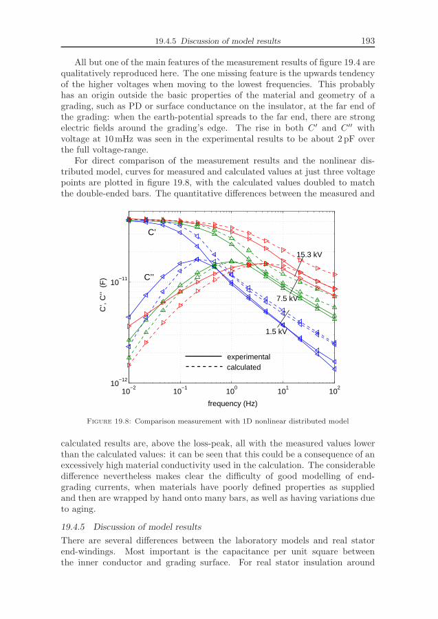
19.4.5 Discussion of model results 193
All but one of the main features of the measurement results of figure 19.4 arequalitatively reproduced here. The one missing feature is the upwards tendencyof the higher voltages when moving to the lowest frequencies. This probablyhas an origin outside the basic properties of the material and geometry of agrading, such as PD or surface conductance on the insulator, at the far end ofthe grading: when the earth-potential spreads to the far end, there are strongelectric fields around the grading’s edge. The rise in both C′ and C′′ withvoltage at 10mHz was seen in the experimental results to be about 2 pF overthe full voltage-range.
For direct comparison of the measurement results and the nonlinear dis-tributed model, curves for measured and calculated values at just three voltagepoints are plotted in figure 19.8, with the calculated values doubled to matchthe double-ended bars. The quantitative differences between the measured and
10−2
10−1
100
101
102
10−12
10−11
frequency (Hz)
C’,
C’’
(F
) C’’
C’
15.3 kV
1.5 kV
calculatedexperimental
7.5 kV
Figure 19.8: Comparison measurement with 1D nonlinear distributed model
calculated results are, above the loss-peak, all with the measured values lowerthan the calculated values: it can be seen that this could be a consequence of anexcessively high material conductivity used in the calculation. The considerabledifference nevertheless makes clear the difficulty of good modelling of end-grading currents, when materials have poorly defined properties as suppliedand then are wrapped by hand onto many bars, as well as having variations dueto aging.
19.4.5 Discussion of model results
There are several differences between the laboratory models and real statorend-windings. Most important is the capacitance per unit square betweenthe inner conductor and grading surface. For real stator insulation around

194 Chapter 19: End-grading currents
the 10 kV level, with a thickness of a few millimetres and relative permittivityaround 4.5, this capacitance is several times higher than for the PTFE tubesof thickness 5 mm and relative permittivity 2.1. Having a larger capacitanceper unit length, without a correspondingly large increase in series conductivity,would shift the qualitative features to lower frequencies. We are not aware ofthe availability of more conductive stress-grading tapes than the one used here,but some other ones have lower surface-conductivity. The paint, even whenquite thickly applied, had lower surface-conductivity.
The most important part of the curves for practical dielectric measurementsseems therefore to be at frequencies above the loss peak. In this range the farend of the grading is scarcely influenced by the potential at the stator end, andapproximations of an infinite length are reasonable. Time-domain spectroscopyon stator insulation has sometimes been used with an assumption of a t−k
behavior of current in the end-winding, which fits with the power-law response inthe frequency-domain [Jon83]. This clearly assumes that the end is not reachedwithin the times used. Dielectric measurements on unguarded new stator coilsrated at 7.2 kV and using the same type of stress-grading tape have only begunto show the loss-peak at the lowest frequency used, 1 mHz. This was at aroundthe rated voltage.
Having a distributed but linear model gave a better approximation at fre-quencies above the loss-peak than a discrete nonlinear model. The linear model,even if conductivity is uniformly scaled as some function of applied voltage,does not however capture how at increasing voltages C′ gets larger than C′′ andtheir gradients get shallower, due to the higher conductivity in the higher-fieldsection at the start of the grading. This behavior of C′ and C′′ corresponds to aincreased slope in the time-domain if using linear power-law models of dielectricresponse.
The noncircular cross-section of stator bars, the proximity of bars from thesame or other phases close to the graded section in an end-winding, and thepossibility of significant dispersion or conductivity in the insulation material, arefurther differences between the laboratory models and real end-windings. Onsimple analyses these are not expected to be at all as important to the relevanceof the presented results as the difference in capacitance discussed above.
Painted stress-grading material can clearly vary a lot in thickness dependingon how it is painted. Even the taped material has been suggested, in theliterature, to vary with age or treatment, and various types are offered by severalmanufacturers. Accurate models of stress-grading currents are not plausible ifneeding to have measured material properties and geometries. It might be thata sufficient model for the substantial removal of the end-winding current in orderto see the current due to PD can be acheived through estimation of the gradingparameters using measurements at sub-inception voltages.
Laboratory models have shown the features of the dielectric response dueto just the geometry and material of stator end-winding stress grading. Theresponse at frequencies above the loss-peak is the most relevant to real end-windings, due to their higher capacitance than the models. At these frequenciesC′ and C′′ at low voltage are similar to the case of a linear distributed-RC
19.5 Measurements on real stator insulation 195
line, giving slopes of −0.5 decades per decade against frequency, but at highervoltages the slopes decrease and C′ exceeds C′′ as the nonlinearity changes theconductivity along the grading.
Towards lower frequencies the displacement current in the insulation underthe grading is so low that the grading’s conductivity starts to influence thepotential at the grading’s far end. This happens more easily if using lowerfrequencies, higher voltages, more conductive grading, less capacitive insulation,or if the grading is shorter. When the grading’s end does become significant thedielectric response changes a lot, with the power-law curves seen for C′ and C′′
at the higher frequencies turning to more Debye-like curves that indicate a limitto the total charge. that can move. The curves for C′ tends to the capacitancethat the whole length of the grading would have if the grading were conductive.As the electric field in the grading material is very low at low frequency, thenonlinearity becomes insignificant and the C′′ curves also converge with eachother as they diminish towards low frequency.
19.5 Measurements on real stator insulation
Measurements on real stator bars were made to see how different the end-winding currents are when the SiC-tape material has been wound on epoxy-micainsulation and treated with VPI, as well as having a different cross-sectionalshape and a different insulation thickness and permittivity. The differencebetween the DS results of the nearly linear slot part alone, then the wholebar with both ends, is also shown, to make clear how great the effect from theend-grading can be.
19.5.1 Dielectric response of end-windings alone
The fundamental-frequency capacitance and loss, including the contributionof the short (≃ 30mm) length of insulation under the electrode, is shown infigure 19.9 for all three of these gradings over a wide range of frequencies.The shorter grading shows the expected tendency to a lower value of low-frequency capacitance, with this and the associated loss-peak happening athigher frequencies than for the normal-length gradings.
The current expected from the electrode was then subtracted from theresults, based on the earlier measurements of the dielectric response of theguarded slot-part that is shown in figure 18.4. Each measured point had asubtraction of the current that had been measured in the slot part at the samevoltage amplitude and frequency, scaled by the electrode length. To measurethe length would have the troubles that the insulation thickness may not be thesame along the electrode as its average value in the slot, so the per-unit-lengthproperties may not be quite right; and the electrode length is not very preciselyknown. Lengths were ‘chosen’, close to the expected values of about 30mm,based on the best fit of the results, giving straight and parallel C′ and C′′ at low-voltage points towards high-frequency. The lengths thus chosen were 29.0mmfor the end of the bar named ‘good’ (because of not having ever had damage toits guard-band), and 28.4mm for the end named ‘bad’ (a repaired guard-band,which seems to have had no effect on the results). The resulting ‘pure’ dielectricresponses seen for the region of the grading material over the stator insulation

196 Chapter 19: End-grading currents
10−4
10−3
10−2
10−1
100
101
102
100
101
102
frequency [Hz]
C [
pF]
0.3 kV
0.3 kV
1.2 kV
4.8 kV
14.4 kV
C’’
C’
14.4 kV
Figure 19.9: The raw (no removal of the capacitance from the electrode) measurements ontwo similar gradings on the guarded bar and the shorter grading () on the samples bar.
material are shown in figure 19.10. The results are very similar in form to those
10−4
10−3
10−2
10−1
100
101
102
100
101
102
frequency [Hz]
C [
pF]
C’’
C’
0.3 kV
1.2 kV
4.8 kV
14.4 kV
lshunt
= 29.00 mm
10−4
10−3
10−2
10−1
100
101
102
100
101
102
frequency [Hz]
C [
pF]
lshunt
= 28.42 mm
0.3 kV
1.2 kV
4.8 kV
14.4 kV
Figure 19.10: Both ends of the guarded bar (’good’ end left, ’bad’ right): C′ and C′′ of thegrading part with subtraction of the addition capacitance from the electrode, based on themeasured properties of the slot part.
from the simpler test objects made from PTFE tubes, although the insulationof the real stator bar has greater variation of its own with frequency. Eventhe low-frequency behaviour of the loss, starting to rise again at the lowestfrequencies, is seen in both cases: this would be more understandable with thestator insulation, where the material under the grading has its own rising loss,but its presence even with the PTFE insulation suggests that, at least in thatcase, it owes more to leakage or discharge around the open end of the gradingthan to the properties of the solid material.
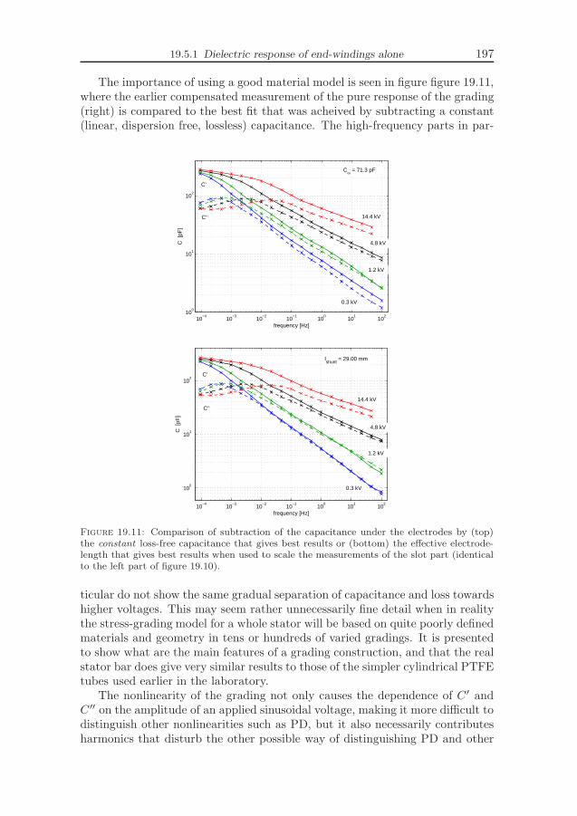
19.5.1 Dielectric response of end-windings alone 197
The importance of using a good material model is seen in figure figure 19.11,where the earlier compensated measurement of the pure response of the grading(right) is compared to the best fit that was acheived by subtracting a constant(linear, dispersion free, lossless) capacitance. The high-frequency parts in par-
10−4
10−3
10−2
10−1
100
101
102
100
101
102
frequency [Hz]
C [
pF]
4.8 kV
14.4 kV
1.2 kV
C’’
C’
0.3 kV
C∞ = 71.3 pF
10−4
10−3
10−2
10−1
100
101
102
100
101
102
frequency [Hz]
C [
pF]
C’’
C’
0.3 kV
1.2 kV
4.8 kV
14.4 kV
lshunt
= 29.00 mm
Figure 19.11: Comparison of subtraction of the capacitance under the electrodes by (top)the constant loss-free capacitance that gives best results or (bottom) the effective electrode-length that gives best results when used to scale the measurements of the slot part (identicalto the left part of figure 19.10).
ticular do not show the same gradual separation of capacitance and loss towardshigher voltages. This may seem rather unnecessarily fine detail when in realitythe stress-grading model for a whole stator will be based on quite poorly definedmaterials and geometry in tens or hundreds of varied gradings. It is presentedto show what are the main features of a grading construction, and that the realstator bar does give very similar results to those of the simpler cylindrical PTFEtubes used earlier in the laboratory.
The nonlinearity of the grading not only causes the dependence of C′ andC′′ on the amplitude of an applied sinusoidal voltage, making it more difficult todistinguish other nonlinearities such as PD, but it also necessarily contributesharmonics that disturb the other possible way of distinguishing PD and other
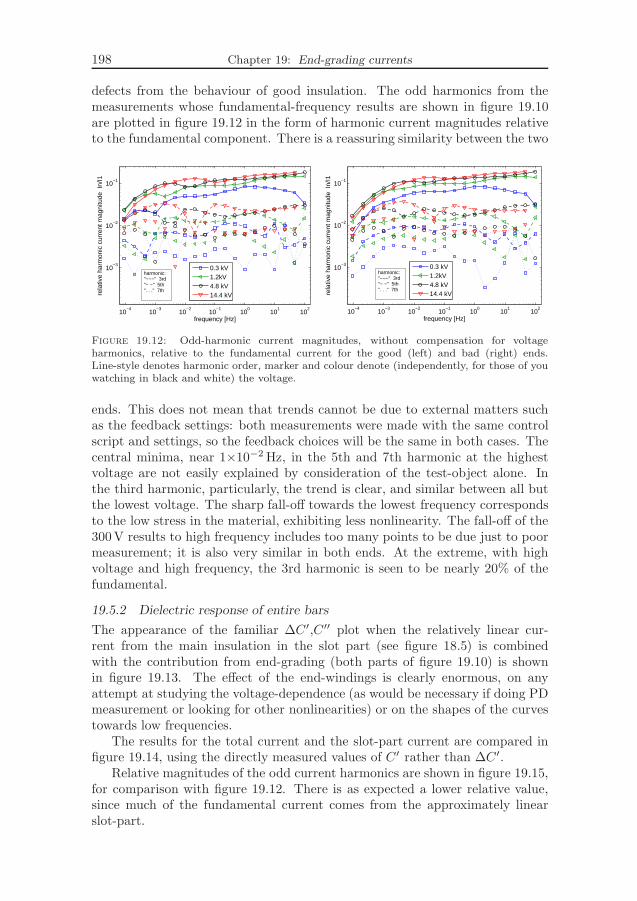
198 Chapter 19: End-grading currents
defects from the behaviour of good insulation. The odd harmonics from themeasurements whose fundamental-frequency results are shown in figure 19.10are plotted in figure 19.12 in the form of harmonic current magnitudes relativeto the fundamental component. There is a reassuring similarity between the two
10−4
10−3
10−2
10−1
100
101
102
10−3
10−2
10−1
frequency [Hz]
rela
tive
harm
onic
cur
rent
mag
nitu
de I
n/I1
0.3 kV1.2kV4.8 kV14.4 kV
harmonic: "−−−" 3rd"− −" 5th". . ." 7th
10−4
10−3
10−2
10−1
100
101
102
10−3
10−2
10−1
frequency [Hz]re
lativ
e ha
rmon
ic c
urre
nt m
agni
tude
In/
I1
0.3 kV1.2kV4.8 kV14.4 kV
harmonic: "−−−" 3rd"− −" 5th". . ." 7th
Figure 19.12: Odd-harmonic current magnitudes, without compensation for voltageharmonics, relative to the fundamental current for the good (left) and bad (right) ends.Line-style denotes harmonic order, marker and colour denote (independently, for those of youwatching in black and white) the voltage.
ends. This does not mean that trends cannot be due to external matters suchas the feedback settings: both measurements were made with the same controlscript and settings, so the feedback choices will be the same in both cases. Thecentral minima, near 1×10⁻² Hz, in the 5th and 7th harmonic at the highestvoltage are not easily explained by consideration of the test-object alone. Inthe third harmonic, particularly, the trend is clear, and similar between all butthe lowest voltage. The sharp fall-off towards the lowest frequency correspondsto the low stress in the material, exhibiting less nonlinearity. The fall-off of the300V results to high frequency includes too many points to be due just to poormeasurement; it is also very similar in both ends. At the extreme, with highvoltage and high frequency, the 3rd harmonic is seen to be nearly 20% of thefundamental.
19.5.2 Dielectric response of entire bars
The appearance of the familiar ∆C′,C′′ plot when the relatively linear cur-rent from the main insulation in the slot part (see figure 18.5) is combinedwith the contribution from end-grading (both parts of figure 19.10) is shownin figure 19.13. The effect of the end-windings is clearly enormous, on anyattempt at studying the voltage-dependence (as would be necessary if doing PDmeasurement or looking for other nonlinearities) or on the shapes of the curvestowards low frequencies.
The results for the total current and the slot-part current are compared infigure 19.14, using the directly measured values of C′ rather than ∆C′.
Relative magnitudes of the odd current harmonics are shown in figure 19.15,for comparison with figure 19.12. There is as expected a lower relative value,since much of the fundamental current comes from the approximately linearslot-part.

19.5.2 Dielectric response of entire bars 199
10−4
10−3
10−2
10−1
100
101
102
102
103
frequency [Hz]
∆C’
& C
’’ [p
F]
0.30 kV
1.19 kV
4.77 kV
14.31 kV
C∞ = 3408pF
Figure 19.13: The complete ‘guarded’ bar, slot and end parts, with removal of a constantestimated C∞.
10−4
10−3
10−2
10−1
100
101
102
3200
3400
3600
3800
4000
4200
4400
4600
C’
[pF
]
10−4
10−3
10−2
10−1
100
101
102
101
102
103
frequency [Hz]
C’
[pF
]
0.30 kV
1.19 kV
4.77 kV
14.32 kV
slotand ends
slotand ends
slot−partalone
slot−partalone
Figure 19.14: Comparison of raw capacitance and loss, (no removal of ∆C′) of the guardedbar with and without the graded ends guarded.
As an example of the variation found between different bars that havesupposedly got the same parameters, figure 19.16 shows the results for measure-ments on the four complete bars without guardbands, described in chapter 18,showing a spread in both C′ and C′′ that is about as much as the differencebetween measurements at different voltage levels.

200 Chapter 19: End-grading currents
10−4
10−3
10−2
10−1
100
101
102
10−6
10−5
10−4
10−3
10−2
frequency [Hz]
rela
tive
harm
onic
mag
nitu
de
0.30 kV
1.19 kV
4.77 kV
14.31 kV
"−−" 3rd"− −" 5th"..." 7th
Figure 19.15: Relative magnitudes of odd harmonics in the measured current in the completebar (‘guarded’ bar) with slot and end parts together.
10−4
10−2
100
102
3800
4000
4200
4400
4600
4800
5000
5200
frequency [Hz]
C’
[pF
]
10−4
10−2
100
102
102
frequency [Hz]
C’’
[pF
]
blue, green, red, cyan: 0.3, 1.2, 4.8, 14.4kVo, x, ^, s: C1l, C1r, C2l, C2r(> is a short, hf re−measurement on C2l)
Figure 19.16: C′ and C′′ from the four complete bars with metal plates along the slot partand no guard-gaps. All had the same sequence, in room-temperature of 22 ± 2 C. Compareto figure 19.14 which gives a clearer view of the curves at different voltages, for just one object.

Chapter 20
SiC-based stress-grading material
The models in chapter 19 rely on a description of the electrical properties ofthe SiC-based materials that form the active part of the stress-grading system.There is insufficient information in the literature on this subject to permitconfident choice of models and parameters.
This chapter describes several groups of measurements that have been madeto establish suitable descriptions of conductivity and permittivity over the rangeof electric fields and frequencies of interest in the models. The main materialstudied was an SiC-based B-stage tape, whose electrical properties have beenmeasured with dc and ac fields, at several temperatures, and on simple tubesand complete stator bars.
20.1 Literature on the material properties
The normal use of stress-grading is simply the prevention of excessive surfacefields, without excessive loss. This puts no tight demand on the properties, andthe materials’ properties are therefore defined only very loosely by manufactur-ers. An example of specifications of three models of stress-grading material canbe seen in [Con05, fig.8].
20.1.1 Models of electrical properties
There is very little in the literature about the desired relations of conductivityand permittivity to electric field and frequency, or about the extent of similar-ity between the different materials available for this application or how theirproperties vary with age. Previous investigations of end-winding grading havebeen interested in the heating-effect of the loss, or the distribution of electricfield, particularly at frequencies much higher than the line-frequency such as forinverter-fed drives [EC05] [Whe07].
Investigations of slot and end-winding corona-protection materials are re-ported in [Eme96], but the emphasis is still on the normal function of thematerial, rather than on modelling of currents over a wide range of amplitudesand frequencies of the voltage. For a density of axial current of about 80 nA/mmaround the circumference, an acceptable range of surface-resistivity is given as2.5GΩ/sq to 4.0GΩ/sq, but the material is not characterised under the widerange of stresses that is needed for modeling of the currents at widely variedamplitude and frequency of the applied voltage.
There is a close relation to the study of grading systems with similar purposein medium-voltage cable terminations, where again the higher-frequency fieldsand heating are the main interest. The cable terminations also use powders,such as carbon-black or SiC, but distributed less densely, in a polymer matrix.
201

202 Chapter 20: SiC-based stress-grading material
Two simple empirical descriptions of conductivity σ as a function of electricfield E are widely found in published models of gradings at cable terminationsand end-windings. One is the power-law or ‘varistor’ equation of the form
σ(E) = k|E|np , (20.1)
used in some works on cable-terminations and end-windings [Ref88] [Rob95][Rhy97] and in a more numerically friendly form with a finite conductivity atzero field in [Lup96]. The other is the exponential relation of the form
σ(E) = k exp(neE), (20.2)
widely used for end-windings [Riv99] [EK03] [EC05] [Dav07] [Min07] and havinginherently good numerical properties of not vanishing at zero field; this has alsosometimes been used for cable-terminations [Qi04].
It is clear that these two types of function cannot be a good fit to thesame data except over a very limited range, yet both are being used in eachof two applications of SiC-based stress-grading. We want to be able to modelthe grading over a wide range of amplitudes and frequencies of the appliedvoltage, so it is important to have confidence that the chosen model is suitable.In [Mar01a] [Mar01b] the electrical properties of SiC powders are studied; thedense nature of stress-grading materials for machines makes the powders morerelevant than for cables; plots of the logarithm of conductivity against electricfield rise more slowly than linearly, suggesting that an exponential function risestoo fast to model the conductivity well. Some of those results are shown herein figure 20.3.
In [Gul00] and some later works citing it, a different form (20.3) is given,having properties that are a hybrid of the power-law and exponential forms:
σ(E) = σ0 exp(
n |E|2/3)
(20.3)
where σ0 is the zero-field conductivity. This is claimed to fit well to a range ofend-winding grading materials, and it has been found to fit well to our results,as will be seen in the later sections. It fits a lot better than either of the purefunctions mentioned earlier. Making the exponent 2/3 variable is sometimes anadvantage.
20.1.2 Complications: further parameters and variation
Bearing in mind the variation that is to be expected between stress-gradingmaterials, due to different specifications, loose tolerance, variations betweenbatches, changes during aging, and differences in processing, it is of interest toknow which parameters of a model are likely to vary much between differentmachines. If, ideally, all SiC-based grading materials varied only in a scale-factor(such as σ0 in (20.3), modelling would be much easier, requiring estimation onlyof this parameter and the length of the grading. Such a convenient situation ap-pears, unfortunately, not to be true. Other possible complications are the effectof other variables on the results, such as effects of frequency and temperature,and anisotropy and inhomogeneity.
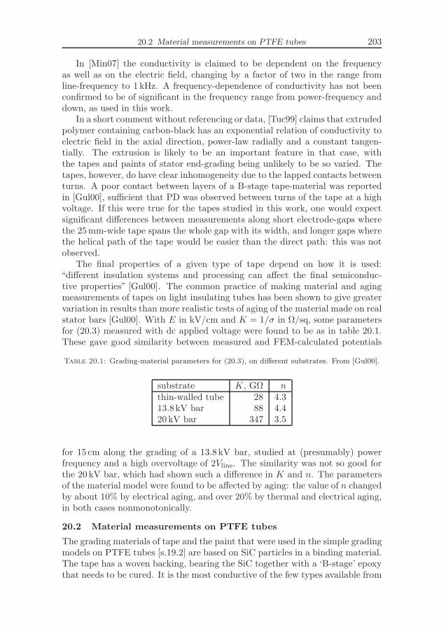
20.2 Material measurements on PTFE tubes 203
In [Min07] the conductivity is claimed to be dependent on the frequencyas well as on the electric field, changing by a factor of two in the range fromline-frequency to 1 kHz. A frequency-dependence of conductivity has not beenconfirmed to be of significant in the frequency range from power-frequency anddown, as used in this work.
In a short comment without referencing or data, [Tuc99] claims that extrudedpolymer containing carbon-black has an exponential relation of conductivity toelectric field in the axial direction, power-law radially and a constant tangen-tially. The extrusion is likely to be an important feature in that case, withthe tapes and paints of stator end-grading being unlikely to be so varied. Thetapes, however, do have clear inhomogeneity due to the lapped contacts betweenturns. A poor contact between layers of a B-stage tape-material was reportedin [Gul00], sufficient that PD was observed between turns of the tape at a highvoltage. If this were true for the tapes studied in this work, one would expectsignificant differences between measurements along short electrode-gaps wherethe 25mm-wide tape spans the whole gap with its width, and longer gaps wherethe helical path of the tape would be easier than the direct path: this was notobserved.
The final properties of a given type of tape depend on how it is used:“different insulation systems and processing can affect the final semiconduc-tive properties” [Gul00]. The common practice of making material and agingmeasurements of tapes on light insulating tubes has been shown to give greatervariation in results than more realistic tests of aging of the material made on realstator bars [Gul00]. With E in kV/cm and K = 1/σ in Ω/sq, some parametersfor (20.3) measured with dc applied voltage were found to be as in table 20.1.These gave good similarity between measured and FEM-calculated potentials
Table 20.1: Grading-material parameters for (20.3), on different substrates. From [Gul00].
substrate K, GΩ nthin-walled tube 28 4.313.8kV bar 88 4.420 kV bar 347 3.5
for 15 cm along the grading of a 13.8 kV bar, studied at (presumably) powerfrequency and a high overvoltage of 2Vline. The similarity was not so good forthe 20 kV bar, which had shown such a difference in K and n. The parametersof the material model were found to be affected by aging: the value of n changedby about 10% by electrical aging, and over 20% by thermal and electrical aging,in both cases nonmonotonically.
20.2 Material measurements on PTFE tubes
The grading materials of tape and the paint that were used in the simple gradingmodels on PTFE tubes [s.19.2] are based on SiC particles in a binding material.The tape has a woven backing, bearing the SiC together with a ‘B-stage’ epoxythat needs to be cured. It is the most conductive of the few types available from
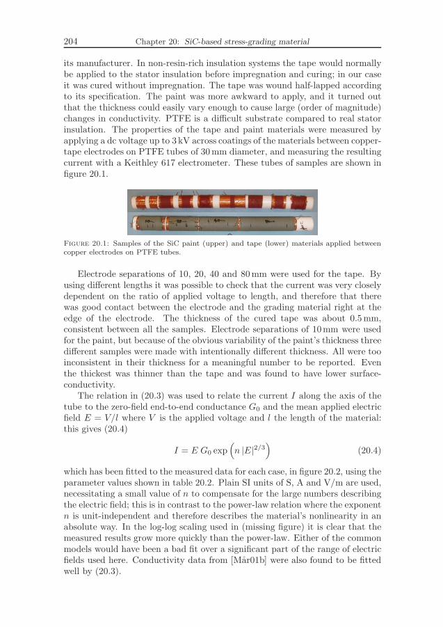
204 Chapter 20: SiC-based stress-grading material
its manufacturer. In non-resin-rich insulation systems the tape would normallybe applied to the stator insulation before impregnation and curing; in our caseit was cured without impregnation. The tape was wound half-lapped accordingto its specification. The paint was more awkward to apply, and it turned outthat the thickness could easily vary enough to cause large (order of magnitude)changes in conductivity. PTFE is a difficult substrate compared to real statorinsulation. The properties of the tape and paint materials were measured byapplying a dc voltage up to 3 kV across coatings of the materials between copper-tape electrodes on PTFE tubes of 30mm diameter, and measuring the resultingcurrent with a Keithley 617 electrometer. These tubes of samples are shown infigure 20.1.
Figure 20.1: Samples of the SiC paint (upper) and tape (lower) materials applied betweencopper electrodes on PTFE tubes.
Electrode separations of 10, 20, 40 and 80mm were used for the tape. Byusing different lengths it was possible to check that the current was very closelydependent on the ratio of applied voltage to length, and therefore that therewas good contact between the electrode and the grading material right at theedge of the electrode. The thickness of the cured tape was about 0.5mm,consistent between all the samples. Electrode separations of 10mm were usedfor the paint, but because of the obvious variability of the paint’s thickness threedifferent samples were made with intentionally different thickness. All were tooinconsistent in their thickness for a meaningful number to be reported. Eventhe thickest was thinner than the tape and was found to have lower surface-conductivity.
The relation in (20.3) was used to relate the current I along the axis of thetube to the zero-field end-to-end conductance G0 and the mean applied electricfield E = V/l where V is the applied voltage and l the length of the material:this gives (20.4)
I = E G0 exp(
n |E|2/3)
(20.4)
which has been fitted to the measured data for each case, in figure 20.2, using theparameter values shown in table 20.2. Plain SI units of S, A and V/m are used,necessitating a small value of n to compensate for the large numbers describingthe electric field; this is in contrast to the power-law relation where the exponentn is unit-independent and therefore describes the material’s nonlinearity in anabsolute way. In the log-log scaling used in (missing figure) it is clear that themeasured results grow more quickly than the power-law. Either of the commonmodels would have been a bad fit over a significant part of the range of electricfields used here. Conductivity data from [Mar01b] were also found to be fittedwell by (20.3).

20.2.1 Temperature-dependence of the SiC material 205
10 100
10−10
10−9
10−8
10−7
10−6
10−5
mean electric field (V/mm)
curr
ent
(A)
30030
tape
thick paint
medium paint
thin paint
2.5−−4.0 GΩ/sq, at 80nA/mm
Figure 20.2: Measurement of dc I/V for samples on PTFE tubes, fitted to (20.4) using theparameters of table 20.2. The horizontal line of ‘2.5 – 4.0GΩ/sq’ is the range given in [Eme96].
Table 20.2: Material model parameters fitting equation (20.4) to (figure ). The unit Sm isintended: it is the conductance of a 1m length. Alternatively: A/(V/m).
Material G0 [Sm] n ρsurf(0) = 2πr/G0
Tape 5.5×10⁻¹³ 0.00115 1.7×10¹¹
Paint (thin) 2.5×10⁻¹⁶ 0.00114 3.9×10¹⁴
Paint (medium) 1.8×10⁻¹⁵ 0.00115 5.4×10¹³
Paint (thick) 1.0×10⁻¹³ 0.00110 9.7×10¹¹
The curves’ parallel appearance makes it clear that the difference, in spite ofthe wide variation in current between the different samples, is due to differencesmainly in the scaling factor G0.
Some models have considered the permittivity of the grading material, too.The permittivity of SiC powders is shown in [Mar01b] to double from a low-field value of relative permittivity of 20, when coming up to 1.5 kV/mm. Inend-winding stress grading the field is generally not above some 500V/mm:at this level the relative permittivity from [Mar01b] is about 30. The datafrom [Mar01b] are plotted in figure 20.3, with the permittivity and conductivityfitted by a linear relation and (20.3) respectively. The voltage-dependence isthus much weaker than for the conductivity. The possibility of a significant andnon-linear permittivity is considered in the model of [Rhy97]. That model, aswith most work on stress-grading, is aimed more at high-frequency phenomenathan at diagnostic measurements. The importance of the permittivity becomesless at lower frequencies.
20.2.1 Temperature-dependence of the SiC material
The temperature-dependence of the SiC material may be important: if it changesmuch in relative value, or changes in the shape of I/V relation, at plausible tem-

206 Chapter 20: SiC-based stress-grading material
0
10
20
30
40
50
0 0.2 0.4 0.6 0.8 1 1.2 1.4 1.6
rela
tive
perm
ittiv
ity
field, kV/mm
C/VAC-pulse
DR16x + 21
1e-09
1e-08
1e-07
1e-06
1e-05
0 0.2 0.4 0.6 0.8 1 1.2 1.4 1.6
cond
uctiv
ity, S
/m
field, kV/mm
C/VAC-pulse
DRI/V
5e-9 exp(3.4 x^0.6)
Figure 20.3: Data for SiC powder, from [Mar01b], fitted with linear relation for permittivityand the exponential-of-power equation (20.3) for conductivity.
peratures for machine measurements, then the likely variation in temperaturebetween practical industrial measurements will affect the goodness of a model.
Measurements of dc I/V relation were made in the 10mm sample on thehollow PTFE samples-tube that was used for the earlier measurements of ma-terial properties. The curves for temperatures from 20 C to 100 C are shownin figure 20.4. The plot against mean electric field shows just the measurements
50 100 300
10−7
10−6
10−5
E [V/mm]
I [A
]
20 40 60 80 100
10−7
10−6
10−5
T [°C]
I [A
]
50 V/mm20°C
100°C
Figure 20.4: The dc I/V relation at temperatures of 20 C to 100 C in 20 C increments. Thedata on the left and right are the same, plotted against the mean field and the temperaturerespectively. Curves between the marked extremes of parameter-values correspond to evenlyspaced changes in the parameter.
taken with rising temperature. The oven† took about ten minutes to do each20 C and get the test-object to a sufficiently constant temperature: the elec-trometer reading at a moderate 500V applied voltage was observed to reacha quite steady value before starting the proper measurement sequence at eachnew temperature. The plot against temperature, on the right, includes also afinal measurement at room temperature of 20 ± 2 C taken the day after, asa check that there was no long-term effect: this point on each curve is linkedstraight to the 100 C point. Given the uncertainty of temperature, and thelower value of the result at the repeated 20 C point, it seems the trend seen
† Weiss 305SB/+10IU/80DU “refrigerated/heated/humidified test cabinet”.
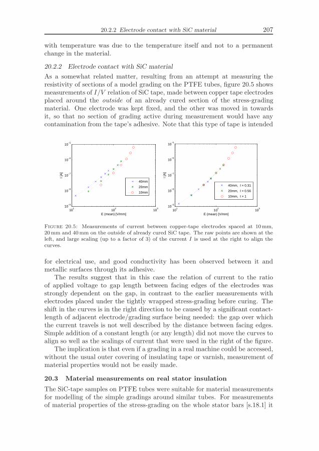
20.2.2 Electrode contact with SiC material 207
with temperature was due to the temperature itself and not to a permanentchange in the material.
20.2.2 Electrode contact with SiC material
As a somewhat related matter, resulting from an attempt at measuring theresistivity of sections of a model grading on the PTFE tubes, figure 20.5 showsmeasurements of I/V relation of SiC tape, made between copper tape electrodesplaced around the outside of an already cured section of the stress-gradingmaterial. One electrode was kept fixed, and the other was moved in towardsit, so that no section of grading active during measurement would have anycontamination from the tape’s adhesive. Note that this type of tape is intended
101
102
103
10−9
10−8
10−7
10−6
10−5
E (mean) [V/mm]
I [A
]
101
102
103
10−9
10−8
10−7
10−6
10−5
E (mean) [V/mm]
I [A
]
40mm
20mm
10mm
40mm, I × 0.31
20mm, I × 0.56
10mm, I × 1
Figure 20.5: Measurements of current between copper-tape electrodes spaced at 10mm,20mm and 40mm on the outside of already cured SiC tape. The raw points are shown at theleft, and large scaling (up to a factor of 3) of the current I is used at the right to align thecurves.
for electrical use, and good conductivity has been observed between it andmetallic surfaces through its adhesive.
The results suggest that in this case the relation of current to the ratioof applied voltage to gap length between facing edges of the electrodes wasstrongly dependent on the gap, in contrast to the earlier measurements withelectrodes placed under the tightly wrapped stress-grading before curing. Theshift in the curves is in the right direction to be caused by a significant contact-length of adjacent electrode/grading surface being needed: the gap over whichthe current travels is not well described by the distance between facing edges.Simple addition of a constant length (or any length) did not move the curves toalign so well as the scalings of current that were used in the right of the figure.
The implication is that even if a grading in a real machine could be accessed,without the usual outer covering of insulating tape or varnish, measurement ofmaterial properties would not be easily made.
20.3 Material measurements on real stator insulation
The SiC-tape samples on PTFE tubes were suitable for material measurementsfor modelling of the simple gradings around similar tubes. For measurementsof material properties of the stress-grading on the whole stator bars [s.18.1] it

208 Chapter 20: SiC-based stress-grading material
should be considered that the stress-grading has been through the VPI process,is in contact with a different insulation and with a binding tape around it, andis not in a cylindrical geometry.
One of the bars described in [s.18.1] had all its outer tapes stripped offexcept the binding tape far in the end-winding region, leaving the plain mica-based main-insulation tapes exposed. It is shown in four pictures, from end toend, in figure 20.6. These new samples differ from the PTFE in being on a real
Figure 20.6: Samples of the SiC tape applied between short electrodes of wire and slot-semiconductor tape along a real stator bar, with the treated with VPI and curing.
bar, with non-circular cross-section and with considerable capacitance to the(floating) central conductor-bundle, and they have been through the VPI andcuring process for the whole insulation system. Some of the samples are alsocovered in the slightly shrinkable insulating binding-tape that is applied to theend-windings of the manufacturer’s machines.
Pairs of electrodes made from the 25mm-thick slot semiconductor tape witha twist of tinned copper (probably) wire beneath, were put along the slot-part,most of them having a sample of the SiC-based tape for end-winding gradingwrapped between them.
Empty electrode-pairs, having just electrodes on the insulation surface, with-out any intentionally conducting material between, were made with 10mm and20mm gaps, were used to give an idea of the capacitance measured in theabsence of stress-grading material.
Electrode-pairs with stress-grading material wrapped in the prescribed half-lapped way around and between them were used to get an estimate of materialproperties of the material: 10mm and 20mm lengths were used to allow judge-ment of how important the contact of tape to electrode was.
Multiple samples of stress-grading material were made, some with and someand without a further tightly wrapped outer tape, to see if it the binding makesmuch difference (the real end-windings are wrapped in this tape, but earliermodels and samples that we have used did nothing to take this into account).Two supposedly identical constructions of each type (combination of length,material, wrapped or not) were used, for assessment of variance.
Some extra test-objects such as two wires placed a little apart under a singleslot-semiconductor tape were also applied, in order to measure the resistanceof the electrodes from the external wires to the bulk of the slot-semiconductortape wrapped around these wires. The electrode resistances were confirmed

20.3.1 Measurements with dc 209
to be trivial compared even to the high-field resistance of the stress-gradingsamples.
Towards each end of the samples bar an ‘end grading’ was added, startingfrom an electrode of a short length of slot-semiconductor, with a guard-electrodeclose by its non-graded end. The active length (length beyond the electrode)of the stress-grading in the construction of the normal coils 9 cm; the endson the samples bar were made with one having twice this active length, theother half of it. The two lengths were to give a good chance of checking low-frequency behaviour with and without the earth-potential reaching to the endof the grading; it was not known in advance quite how easily this would happen,but only that 1mHz 10 kV (?) measurements on some earlier bars (2006) hadshown only a hint of loss-peak.
20.3.1 Measurements with dc
Figure 20.7 shows the results from dc measurements on all six samples, usingthe same supply and electrometer as for the samples on the PTFE tube, andtherefore limited to 3 kV. Bearing in mind the obvious sources of variation, in
101
102
103
10−9
10−8
10−7
10−6
10−5
E [V/mm]
I [A
]
10mm bound [i]
10mm free [i]
10mm bound [ii]
10mm free [ii]
20mm [i]
20mm [ii]
E k exp(n Ep)
line (Eq)
Figure 20.7: I/E relations with dc, for the six samples of SiC tape between electrodes on abar surface.
particular the tightness and lapping (amount of overlap) of the tapes, besidesvariation in actual electrode separation and in material properties of differentpieces of tape, the similarity between the samples is good. The 20mm samplesshowed no obvious deviation from the 10mm samples in their I/E relation,suggesting that the contacts are of little importance compared to the ‘active’part of the SiC between the electrodes. The trend is certainly not a power-law(straight line) but is much better fitted by the familiar
I = Ek exp (n|E|p) , (20.5)
although appearing better in this case with an exponent p rather closer to 1/2than to 2/3. It does in fact seem that this exponent is less critical to the fit
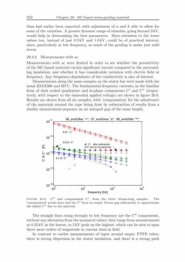
210 Chapter 20: SiC-based stress-grading material
than had earlier been expected, with adjustment of n and k able to allow forsome of the variation. A greater dynamic range of stimulus, going beyond 3 kV,would help in determining the best parameters. More attention to the lowervalues too, instead of just 0.5 kV and 1.0 kV, could be of practical interest,since, particularly at low frequency, so much of the grading is under just mildstress.
20.3.2 Measurements with ac
Measurements with ac were desired in order to see whether the permittivityof the SiC-based material carries significant current compared to the surround-ing insulation, and whether it has considerable variation with electric field orfrequency. Any frequency-dependence of the conductivity is also of interest.
Measurements along the same samples on the stator bar were made with theusual IDAX300 and HVU. The fundamental-frequency currents, in the familiarform of their scaled quadrature and in-phase components C′ and C′′ (respec-tively, with respect to the sinusoidal applied voltage) are shown in figure 20.8.Results are shown from all six samples, with ‘compensation’ for the admittanceof the materials around the tape being done by substraction of results from asimilar measurement-sequence on an untaped gap of the same length.
100
101
102
103
10−16
10−14
10−12
10−10
10−8
frequency [Hz]
06_end10ba: "+"; 07_end10ua: "s"; 08_end10bb: "^";
C’ &
C’’
[F
]
all C’, after subtraction of C’ due to uncoated bar
0.6 kV C’’
6 kV C’’
0.1 kV C’’
Figure 20.8: C′′ and compensated C′, from the three 10mm-long samples. The‘compensated’ points have had the C′ from an empty 10 mm gap subtracted, to approximatethe added C′′ due to the material.
The straight lines rising strongly to low frequency are the C′′ components,without any alteration from the measured values; they range from measurementsat 0.25kV as the lowest, to 5 kV peak on the highest, which can be seen to spanthree more orders of magnitude in current than in field.
In contrast to earlier measurements of tapes around empty PTFE tubes,there is strong dispersion in the stator insulation, and there is a strong path
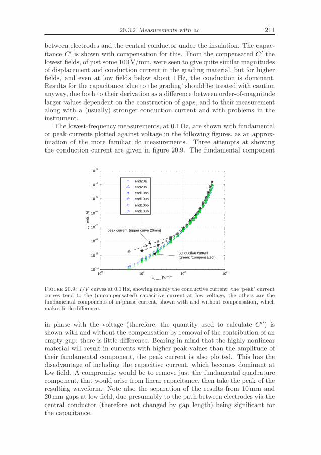
20.3.2 Measurements with ac 211
between electrodes and the central conductor under the insulation. The capac-itance C′ is shown with compensation for this. From the compensated C′ thelowest fields, of just some 100V/mm, were seen to give quite similar magnitudesof displacement and conduction current in the grading material, but for higherfields, and even at low fields below about 1Hz, the conduction is dominant.Results for the capacitance ‘due to the grading’ should be treated with cautionanyway, due both to their derivation as a difference between order-of-magnitudelarger values dependent on the construction of gaps, and to their measurementalong with a (usually) stronger conduction current and with problems in theinstrument.
The lowest-frequency measurements, at 0.1Hz, are shown with fundamentalor peak currents plotted against voltage in the following figures, as an approx-imation of the more familiar dc measurements. Three attempts at showingthe conduction current are given in figure 20.9. The fundamental component
100
101
102
103
10−10
10−9
10−8
10−7
10−6
10−5
10−4
10−3
Emean
[V/mm]
curr
ents
[A]
end20a
end20b
end10ba
end10ua
end10bb
end10ub
peak current (upper curve 20mm)
conductive current(green: ’compensated’)
Figure 20.9: I/V curves at 0.1Hz, showing mainly the conductive current: the ‘peak’ currentcurves tend to the (uncompensated) capacitive current at low voltage; the others are thefundamental components of in-phase current, shown with and without compensation, whichmakes little difference.
in phase with the voltage (therefore, the quantity used to calculate C′′) isshown with and without the compensation by removal of the contribution of anempty gap: there is little difference. Bearing in mind that the highly nonlinearmaterial will result in currents with higher peak values than the amplitude oftheir fundamental component, the peak current is also plotted. This has thedisadvantage of including the capacitive current, which becomes dominant atlow field. A compromise would be to remove just the fundamental quadraturecomponent, that would arise from linear capacitance, then take the peak of theresulting waveform. Note also the separation of the results from 10mm and20mm gaps at low field, due presumably to the path between electrodes via thecentral conductor (therefore not changed by gap length) being significant forthe capacitance.

212 Chapter 20: SiC-based stress-grading material
20.4 Summary
The exponential-of-power equation (20.3) using an exponent 2/3 gives a good fitto the measured dependence of conductivity on applied field, for the SiC-basedstress-grading materials examined here. The 2/3 is not definitely the best choice;The variation in samples due to how the tape is applied puts a limit on howgood a fit it is meaningful to pursue. It seems that many old hydro-generatorshave painted stress-grading, which is likely to lead to even larger variations.
The conductivity has a dominant current over the permittivity, except atthe highest frequencies and lowest fields considered here. The permittivity hasrelatively small variation with field, which based on the measurements andreferences appears to be up to about a factor of two, rather than of severalorders of magnitude for conductivity, up to the maximum expected fields ofaround 0.5 kV/mm. In the real applications, the permittivity is in parallel withother permittivities in the insulation and air, while the conductivity of the SiCmaterial is the main conductive path, so the field-dependence matters still less.
Temperature can change the conductivity considerably at low fields, butvery little at the high fields. The 20 C variation that one might reasonably findbetween different industrial measurements affected the low-field conductivity inthe order of ten percent.
For models of stress grading aimed at the current in low-frequency mea-surements, rather than the field during power-frequency and high-frequencyexcitation, the material measurements suggest that the modelling of the materialby just a nonlinear conductivity is a good approximation. This is confirmed bythe grading models and measurements.
Chapter 21
Conclusions
21.1 Main results
21.1.1 PD measurement by DS
The DS instrument measures the total charge input reliably even when thisarrives as sharp pulses [s.14.2], provided that feedback components are suitablyset to avoid overload. The currents due to PD events within a test-object aretherefore included in the DS results. The DS instrument can give remarkableconsistency of measurements in spite of changes of feedback components, elec-trometer voltage, and frequency, as shown on a gas capacitor [s.12.6]. Given atest-object that is linear apart from PD, the current from a DS measurement ata voltage below PD inception should be able to be scaled and subtracted fromthe current in a high-voltage measurement to give a good approximation of thetotal current due to PD [s.17.1].
21.1.2 PD charge by DS or PD-pulse
There are several reasons why the total PD charge measured by DS and by PDmethods becomes very different as one moves to larger or more PD-intensiveobjects. The complementarity of these measurements may be useful whencombined with the DS system’s measurement of harmonics, as a way to seethe phase-distribution of the whole PD charge as well as seeing the PD patternsthat distinguish individual pulses but miss a lot of pulses in doing so.
21.1.3 Stress-grading response
Measurements on real stator bars have shown that, particularly at high voltage,the loss-peak in the dielectric response is well within the frequency range ofinterest, not below it as had been concluded as likely in [Tay06]. This makesit even more important to consider these models of the response instead of thesimple models that have been popular in studies at relatively high frequencies.
21.1.4 Frequency-dependence of PD
An aspect that has not received much attention here is the frequency-dependenceof pure PD-pulse measurements on stator insulation. This has some promisefor distinguishing PD sources: it seems for example likely that delaminationsmight be more readily distinguished from voids with varied frequency, and thatthis is an important distinction to make. A problem is the need for only alow-frequency range, such as under 1Hz, when measuring on large capacitanceslike a stator winding, at high voltage. Several cycles, preferably tens, would beneeded at each point, and each cycle would take one or many seconds. Thismay be impractically time-consuming.
213

214 Chapter 21: Conclusions
21.2 Suggestions for future investigation
The following are some directions that would be natural continuations of thiswork, without opening completely new branches.
21.2.1 Frequency-dependence
The dependence of common PD sources in stator insulation on the frequencyof the applied voltage has not yet been studied in detail. Up to now thesematters have been displaced by investigations of similarity and differences ofDS and PD, partly because there already have been studies of PD frequency-dependence going on within the research group. It would be good to makeVF-PRPD measurements on some well-defined examples of common stator-insulation defects. It would be of particular interest if defects with significantlydifferent prognostic implications can be shown to give reliably different resultswith variable frequency methods but not with conventional measurements at asingle frequency.
21.2.2 Simultaneous DS and PD on whole windings
Some theoretical attention has been given to measurements on whole statorwindings, but so far the simultaneous, varied-frequency measurement of DSand PD has only been applied to single bars in the laboratory. It would begood to make measurements on a whole stator. The difference between PDmeasurement by DS and PD-pulse methods is expected to be much greater on awhole stator than in the laboratory, owing to the matters of pulse propagationand far larger total number of PD sources, besides the greater likelihood of glow-type PD in highly aged cavities than in quickly aged specimens in the laboratory.The differences such as solid earthing and long distances for connecting cablescan be expected to make the PD pulse method have even greater troubles ofdeadtime and calibration, but might also have adverse effects on the combinedmeasurement.
Although the references in section 8.4 give a thorough study of pulse propa-gation in stator windings, it would also be good to witness the results obtainedwith calibration pulses injected on opposite ends of the winding. One cannotproperly verify subtraction of end-winding currents in the whole stator, sincethe very trouble about these currents is that they cannot be practically guardedaway. The results from attempts at parameter-fitting from voltages below PD-inception would be interesting to see anyway.
21.2.3 Parameter estimation for end-grading models
If end-winding grading models are to be used seriously, in removing some of thedisturbances in measurements of total PD charge, some more attention shouldbe given to estimation of material and geometry parameters. It is clear thatthe variations between different machines, or even the individual bars studied inthis work, can be enough to change a model’s results by an amount that wouldcorrespond to a large error in the calculated PD current.
The possibility of estimating parameters from measurements made at volt-ages below PD-inception is of interest, as a way of avoiding the variation between
21.2.4 Study of service-aged bars 215
different machines, degrees of aging and temperature. As with any estimationor fitting problem, it is useful to restrict the fitted variables by establishing someparameters as being either constant or of a limited range.
Relevant investigations to enable this include the following: How variedare the materials between being new, impregnated, cured and aged? Whatvariations are there between different manufacturers’ materials? How muchdo applied thicknesses vary, and how well can differing parameters on parallelend-winding gradings within a stator be aggregated?
21.2.4 Study of service-aged bars
Measurements could be made on naturally aged bars from old machines, possiblyfollowed by breakdown tests. Breakdown tests cannot be taken as a directmeasure of the lifetime an object might have had in service, but there is noobvious better method of comparing quality within acceptably short times.
The natural aging, compared to very unnaturally accelerated aging that isthe alternative if starting with new bars, would arguably make the results moremeaningful as tests of the diagnostic value of the proposed methods,
21.2.5 Ignoring or estimating the fundamental current
The mixture of large currents from an approximately linear system of solidinsulation, together with smaller but much more strongly nonsinusoidal currentsfrom PD and stress-grading, suggests the possible advantage of using just themeasured harmonic currents.
The fundamental component might be ignored, or might be estimated fromthe harmonics on criteria of physical plausibility. For very large linear currentsfrom the bulk of the insulation, that swamp the small currents from PD or othernonlinearity, this may be more reliable than trying to compensate the disturbingcurrent by subtraction, since small relative errors in the estimated value beingsubtracted could be large errors relative to the small harmonic currents.
21.2.6 Time-sequence, and non-sinusoidal excitation
This work considered only sinusoidal voltages for excitation, and gave resultsof DS current and PD charges only with respect to phase, aggregated over allmeasured cycles.
More versatile measurements can preserve details of the current and PDpulses within time. This is very sensible, as the phase-based methods of thiswork can be immediately derived from the time-based results, but the time-sequence includes extra information.
The applied voltage could use nonsinusoidal waveforms, whether steps, ramps,or more complicated patterns. This might be chosen to show up a particulartype of PD source or to allow easier analysis.
In order to make investigation of these extra details feasible it would benecessary to simplify some other features of the measurement: there is a re-markable amount of data to consider even from the input variables of amplitudeand frequency of the applied voltage and the output variables of harmonics andvarious PD statistics.

216 Chapter 21: Conclusions
Another sort of excitation is a sinusoid superimposed on a quasi-dc level.This has the virtues of high stress on the insulation, low current-demand fromthe source, and separation of conduction and displacement currents in themeasurement. Some work on non-sinusoidal excitation has already started in arelated project within the department.


Appendix A
Principles
This chapter is a mixture of threads that have some connection to the process ofusing reference sources, performing calculations such as computer simulations,designing and conducting experiments, analysing results, drawing conclusions,and presenting results. The subjects were inspired by experiences with labora-tory work and computing, and by reading around for ideas about better waysof working, particularly in experimentation and programming. In some waysthis is an explanation of methods adopted in this work, or a defence of caseswhere a common recommendation or practice has been flouted. In others itis a suggestion that, probably, many people would benefit from learning andthinking about the different focuses and attitudes found in other subject-areas,and the wide range of available methods and tools. It is hard to bring all theseideas together coherently: the result is nowhere near the original aspirationsfor breadth and clarity, yet it feels disturbingly long and often rather trite. Itis included as an appendix in the hope that it will be appreciated by someonefor providing a new idea, an interesting reference, or just a general stimulus toconsider better working-practices.
A.1 Precision of expression
If a statement can be changed to make it more easily tested or challenged,it probably should be changed. Although the virtue of precision is obviousin principle, its practice requires effort in gathering the necessary evidence orformulating the statement, and it is therefore all too easily avoided. It is goodfor the experimenter, reasoner or writer to be forced to think in detail, ratherthan to risk glossing over an assumed or neglected detail . . . but it does takelonger.
A.1.1 Numbers
Statements such as“there was a large increase in resistivity after aging”or“therewas a considerable difference”are common, but are so vague that a reader mightin some cases not be able to infer the actual values within an order of magnitude.Numbers and ranges make the claim far more useful, even if still as vague as“approximately doubled” or “a difference of some 5% to 10%”. Making thesetighter claims often requires going back to the data to check more thoroughly.
The principle of thinking-in-numbers should extend also to the case whereresults deviate from expectations: it is all too easy to dismiss such a deviationas being “probably due to . . . ”, without analysing carefully the consequences ofthat conjecture’s truth so as to check that the supposed explanation is at leastquantitatively plausible. Many times in this work a peculiar result has seemedalmost forgivable, but has been probed further and eventually found to have an
219
220 Appendix A: Principles
error of settings, equipment or analysis lying behind it. Even apparently goodresults are worth checking in several ways, since the belief of goodness mayresult from a double error, something that has happened surprisingly often.
A.1.2 Equations
If an equation can be used instead of the wordy alternative, this will often bepreferable. Forcing the writer to formulate the idea more precisely can show upweaknesses in understanding or definition, and an equation is generally moreaccessible and memorable to a technically minded reader.
A derived equation can so easily have an error, such as a wrong sign, thatsimple checks should be made. There are the simple methods of checkingthe correct response to “x goes up, y comes down” or “what should y do asx → 0”, or dimensional consistency. Computers are helpful too: a derivedanalytical solution can be plotted against a more simply programmed numericalapproximation to reveal errors, and computer-algebra programs can discover theslips that creep into pen-and-paper working.
A.1.3 Sensitivity
Sensitivity analysis considers how much a change in one variable would affectanother. This is clearly strongly relevant in experimental design and analysis[s.A.2], but it should be considered in all manner of situations where differencesor similarities in values prompt a conclusion that may turn out to have beenstrongly influenced by apparently modest disturbances, or to be true only underspecial conditions of other variables that were not identified as being important.
A.1.4 Examples
Even in matters that cannot be clarified by numbers or equations, more claritymight be given to statements by using concrete examples of the implication ofstatements. The phrases for example and such as may become a little tedious,particularly later in this chapter [s.A.2], but it is hoped that they make thepoints much clearer.
A.1.5 Graphical presentation
Graphical information such as pictures, drawings, diagrams and graphs, canserve enormously to clarify an explanation. More should doubtless have beenused in this thesis, but unfortunately the clearer, more precise, often better formof presentation can take a long time to plan and produce.
Diagrams can help a whole set of interlinked thoughts to fasten clearly inthe reader’s mind, as well as showing up defects in the writer’s mental modelby forcing claims to be stated in so explicit a way. They can be useful forshowing how concepts fit together, as well as for the obvious technical cases ofrepresenting circuits and constructions. That they are so time-consuming is in away a consequence of their goodness: by being able to imply so many relationsin a small space, there are many ways in which they can seem slightly wrongand in need of revision.
Graphs of data can greatly increase how much information can be digested.Trends and outliers can be seen that would be unnoticed from tabular numbers.
A.1.5 Graphical presentation 221
Even a function that could be written as an equation may benefit from beingpresented in a graph as well, to clarify its nature and allow comparison withothers. An example of a work with highly graphical and effective presentation ofideas and data is [Mac03]. As with diagrams, it is often hard to decide the best,clearest way of making a graph, and it can be surprisingly time-consuming.
Some ‘good practices’ in graphing are included in [Kir09], with generaland technical examples that extend even to a mention of Paschen’s law. Thefollowing are a few points most relevant to technical use of graphs: rather thanplotting data in its raw form, scaling should be used to show the deviation froman expected relation, making it clearer whether the deviation is largely noise oris a particular trend; a key or legend is commonly used to label the symbolsused for each data-set, but if it is possible to include direct labelling next tothe data, this can make the plot more easily accessible; extra lines such as grid-lines and a box all around a plot are probably rather over-used; ‘joining thedots’ with lines between data-points is by no means always a good idea, and isinappropriate for some types of data.
The scaling of data is widely used in the sorts of subjects considered in thisthesis; indeed, graphs of capacitance are an example of a current being scaledby voltage and frequency in order to show the important trends more clearly.Many graphs could be improved by more work on replacing keys with labelsdirectly by the data; the increased time, particularly if a graph is re-plotted,is the major reason against this good idea. The extra clutter of grid-lines hasoften been accepted, to make it easier to judge gradients, which are particularlyimportant in graphs of capacitance and loss. The data-points in graphs haveoften been joined, for reasons discussed below.
It is clearly desirable to show the actual measured or calculated points on agraph, rather than just a fitted curve, unless there are so many points that therewould be negligible space between them. Many experimentally based worksshow only the points, in order not to make any suggestions about what wasnot studied; an example is [Hel00]. But when plotting several data-sets on onegraph, it can be helpful to have at least a weak line joining the points of each set,to clarify their relation. Some data can meaningfully be interpolated betweenthe measured or calculated points; an example is the variation of capacitanceor loss between closely-spaced frequencies, where joining helps the reader tomake this interpolation. Other data, such as the harmonics of a periodic signal,cannot meaningfully be interpolated between points; even so, connecting thepoints of each data-set can make it easier to distinguish the sets. Bar-charts orunjoined points were used early in this work when trying to display harmonicvalues against harmonic order in the ‘correct’ non-interpolated way, with onedata-set for each of several combinations of voltage amplitude and frequency;the results were much less clear in this way than with simple points and lines.
The display of intervals instead of points is useful for indicating a range ofestimated error or variance; this is considered in [s.A.2.7], as it is connected tomore general presentation of data than just graphs.

222 Appendix A: Principles
A.2 Comparison of ‘research methods’
Scientific investigations are made of many various phenomena, for many reasons:it is no surprise that many different methods are used, and that researchers indifferent areas have little in common in their opinions about the most crucialconsiderations in experimentation and inference. Reading about ‘experimentaldesign and analysis’ in several areas, it seems that the types of problems andmethods often fit into one of a few broad categories, between which there islittle similarity in the approach.
Some of the differences in methods can be explained by differences in thestudied phenomena and disturbances, or differences in the intended applicationof the results. Other differences, however, may be due only to the backgroundsof people working in the different areas, or to historical matters such as long-established methods developed before improvements in concepts or apparatus.The methods in common use in any area are therefore not necessarily the bestones available, and it may be worth investing some time in learning about themethods used in other areas with related problems. The ‘tree’ of all the areas,subareas and so on must have many leaves that in spite of being far from eachother are trying study and solve very similar problems; there might be usefulexchanges between them if only they knew of each other’s existence.
This section compares the phenomena, aims and commonly used methodsin several areas, and briefly considers their potential usefulness in the generalareas of DS, PD and reliability. There is no claim of covering the many areasand methods completely or fairly. An area may have subdivisions that fit intovery different classifications. Areas change over time; biology, for example, hasin the last century changed from a focus on classification† to detailed molecularknowledge and heavy computation. The terminology here may seem a littleforced, from trying to be general enough to describe investigations in suchareas as dielectrics, astronomy, reliability and psychology. Examples of thegeneral term and (typical term in our area) are observation (measurement) anddisturbance (noise or error). Also, ‘controlled’ is used in the sense of beingregulated, nothing to do with a ‘control group’ as a base-case for comparison ofresults.
A.2.1 Aims
The aim of an investigation may be simply to present early results in an easilyaccessible way for other people to study; even in this case there are many choicesto be made about how to display and compare results, and how to show thelikely ranges of measurement-errors or variation between specimens. Anothertype of aim is to estimate a constant, or to describe the functional form of arelation between variables. Other aims may be more clearly related to the thestandard description of testing a hypothesis.
The form of such hypotheses is very varied. Fundamental classical physics istypified by hypotheses in the form of equations that claim a precise law aboutthe relation of several variables; a single demonstrable exception, anywhere, atany time, would require a revision of the law or a restriction of its scope. At
†There are two forms of science: physics and stamp-collecting. — Ernest Rutherford.

A.2.2 Disturbances 223
a less fundamental level, a choice may have to be made between hypotheses ofcompeting models, from which the one best describing the data must be selectedeven if it is clear that none of them gives a very good description. A differentform of hypothesis is “Mars has at some time supported life”, which would bevalidated by a single discovered confirmation; this is admittedly more a matterof history than of the predictive statements normally associated with science.Studies of subjects with lots of variation, such as people, may be content withthe hypothesis that a controllable variable does have some observable effect, or(noncausally) that a particular population does possess a particular property.In either case the result is likely to be sufficiently noisy that a modest proportionof investigations giving opposite results to the rest would more likely be treatedas the result of noise than as indicating errors in the studies or a need for arevised hypothesis; such areas are sometimes called soft sciences.
The steps between the observations that can be made and the result atwhich the investigation is aimed can be complex, requiring a lot of thought andcalculation. Some material properties may be measured quite directly, with themain complexity being the possible treatment of noise; but if observations areto be used to select the most suitable of several models of the underlying causes,a lot of computation may be needed.
An investigation must often be of a causal relation, since this is what isimportant in many practical applications where the results will be used to decidehow to control a phenomenon. The variable whose effect is to be studied mustthen be controlled [Pea00, p.43], unless one is content with correlational studiesand dependence on further assumptions.
Absolute values, or in other words values relative to an accepted reference,are necessary in some cases such as characterisation of materials, for comparisonwith other work. In other cases, such as studying differences between differentlytreated groups of people, or the peak positions of a dielectric response, only therelative values within set of measurements are important.
With such variation in aim between subject-areas, large differences canbe expected in their methods of setting up experiments and analysing andpresenting the results.
A.2.2 Disturbances
In the simplest sort of investigation, observations of a phenomenon could bemade without significant influence of measurement errors or disturbances, andthe results would need little or no processing to achieve the aim. Many factorsconspire to make actual investigations more complex: the following list attemptsto be general enough to be relevant to all areas, even if some of them normallygroup disturbances differently.
Observations of physical phenomena have a limited accuracy.† Errors arise
† Here, accuracy is how close a result is to the true value, the difference being error. Theseare obvious notions in numerical computing, but are often disliked in physical situationswhen the true value is not measurable, particularly when fundamental physical uncertainty isrelevant. They are accepted here as useful notions for many cases, where a true value can beapproached much more closely by the best available methods than by the methods actuallyused under the constraints of time and cost.
224 Appendix A: Principles
from external disturbances that affect the path from the object being studied,and from imperfect calibration of instruments or variability of judgements madeby human observers. Examples are thermal noise, externally-coupled noise,uncompensated parasitic impedances in measurement-circuits, instruments withpoor linearity or poor calibration, differences between the people making as-sessments of the conditions of patients, or incomplete gathering of a crop-yield. Important features of error sources are whether they are constant, followsome function or are random,† and whether they tend more to be additive ormultiplicative in their effect.
Other variables may need to be controlled, or at least known through ob-servations, while observing the main result. Examples are the time at whichan astronomical observation is made, the temperature at which a material-measurement is made, the dimensions of a sample, or supposedly relevant fea-tures, such as age, of people on whom an experiment is performed. Errors inthe measurement of these variables can arise from the same sources as for themain observed variable.
The object being investigated may also vary in ways that are not fully knownto the experimenter. The problem is most obvious when the properties of aclass of object are to be determined; different objects within that class givesomewhat different results, necessitating measurements on more than one tomake the result sufficiently representative. Examples are the establishment ofa relation between a diagnostic result and later failure, estimates of materialproperties from samples, and tests of medical treatments on people.
If the properties of a particular object alone are important, as for a diag-nostic measurement on a particular stator, there is not the need for these extrameasurements to confirm that the object is representative of its kind. Theremay, however, be variations of the observed variable between repetitions of themeasurement, not easily explained by error in the control or observation of othervariables. An example is how PD can change in time due to the complicatedinternal states involved in the phenomenon. Several measurements may then beneeded anyway, to give confidence in the result.
Some types of object can only be used once. This makes it necessary touse different objects for the measurements made at different levels of controlledvariables, which introduces extra disturbance due to the variation between theobjects. This is the case for samples used for destructive tests of insulation, orfor samples that will be compared after being prepared with different additives;it is a very common situation in experiments on living things. An examplewhere the object can be used many times is a piece of insulation having DSmeasurements made at many frequencies of a mild voltage.
A.2.3 Classes of subject-area
The following paragraphs give a very general classification of some differentsubject-areas, based on the sorts of differences in phenomena and aims outlinedabove. There will doubtless be plenty of omissions, over-simplifications andexceptional subareas, but there are several clear groups.
† Unpredictable at each moment, so best described by a statistical distribution.
A.2.3 Classes of subject-area 225
At one extreme are areas that are ‘noisy’ due to variation between objectsand to poorly controllable disturbances: examples are agronomy, medicine,psychology, economics and sociology, as well as reliability within engineering.The classic situation is that the effect of a controllable variable on an observedvariable is to be determined, on objects such as plants, people or products. Thenoise may well cause a variance in results that is greater than the mean effectof the controlled variable under study.
In a simple case the controlled variable has just two levels, such as thepresence or absence of a recommended amount of some nutrient or drug, ortwo constructions of a prototype. The large degree of disturbance necessitatesmeasurements on many samples at each value of the variable in order to make aconfident claim, but the cost of each sample can be high: production of proto-types for destructive testing is expensive; there may be few patients needing aparticular treatment; experiments may have timescales of months or years. Thesmall effects against strong noise also make it necessary to compare groups ofobjects with and without some treatment, rather than comparing results froma treated group with an accepted ‘usual value’.
The potential application of the results can be large, if applied to all thesubsequent production of a product or to choices concerning a whole population,so it is of great utility to detect even a small effect of the controlled variable.In these areas, therefore, ‘statistical’ methods are widespread, to identify smalleffects against the noise and to optimise experiments from the beginning toproduce sufficient information using a minimum of samples.
The science of statistics has been developed for the purpose of assistingin the separation of chance effects from true regularities.[BW52, p.169]
At another extreme are some parts of the physical sciences, opposite inalmost every respect. An example is DS measurements on well-defined linearsubstances: any number of measurements can be made on the same sample,and effects from previous measurements can be largely predicted or avoided;given good shielding and some sort of averaging, the resulting signal can bevery strong compared to the noise; measurements are typically made over manyfrequencies, with the smoothness of the results giving a good indication of thedegree of noise; before seeing the results there will already be a good idea of areasonable range; it is likely to be well known, even quantitatively, which othervariables, for example temperature, are significant.
These features are clearly easier to work with than those of noisy areas,but there are often much higher demands upon the results. In some areas,great attention may be paid to dealing with relatively small levels of noise,and results may have to be accurate relative to a remote standard ratherthan just to other locally measured results. Physical constants are determineddown to many significant figures. Effects of controlled variables are studiedhighly quantitatively, and models have to reproduce them well besides beingappealingly simple. Getting the results in the first place may involve veryclever and complex work with instruments and test-arrangements, rather thanthe opposite extreme of a ‘yes’ or ‘no’ answer in a questionnaire. In these areas,

226 Appendix A: Principles
methods described as ‘error analysis’ are common for simple treatments of theresults, assessing the combined effect of the many sources of error.
The following quotation is an amusing example of how a principle held asimportant in one area may be irrelevant or contrary to another. The firstsentence is a principle of areas with strong noise and statistical analysis: in adata-set with several variables there is a good chance that some pair of variablescan be found between which the noise has caused an apparently significant effect;hence the insistence on advance declaration.
. . . experimental data can never be used as evidence for hypotheses whichwere not listed in advance of the experiment.In physics, at least, exactly the opposite viewpoint is often expressed.If a given interpretation of the data was not thought of until after theexperiment, this is often put forward as evidence that the experimentalresults could not have been influenced by bias in favour of the theory.[BW52, p.294]
Although the physics-like view is appropriate for much of this work, the ability tofool oneself in reliability studies, with noisy results of several variables measuredon small numbers of objects, should be kept in mind.
Moving away from the traditional extremes, there are other noisy areas thatuse methods more commonly described as signal-processing than as statistics.The noise is often from external disturbances and instruments: it may be muchgreater than the signal of interest, as in the traditional noisy subjects, butthe aim typically demands extraction of much more detailed information thanthe presence of a ‘significant difference’ between groups. Examples are modernastronomy, wireless communication, detection of targets by radar, processing ofNMR data [Bre88], and particle physics experiments. Most of these situationsare quite recent, as automation has made it feasible to collect and process enoughdata to provide useful results in spite of the noise.
Such problems are attacked with methods that are suggestive of workerswith wide-ranging backgrounds: for example, Fourier and related analyses,Bayesian inference, information theory, orthodox statistics, and ‘learning’ net-works. Methods capable of such complex tasks can, at best, be general enoughthat the methods of other areas, such as error analysis and orthodox statisticaltesting, are just special cases [Jay03].
A.2.4 Classification of this work
In insulation diagnostics based on the types of method considered in this work,there are several very different subdivisions of the subject-area.
Prognoses are the ultimate aim [s.4.1] of diagnostic measurements; the areaof engineering-reliability, which deals with prognoses, has been seen [s.A.2.3]to have many features of a noisy area. Results from historical operation-dataof equipment, and from experiments with varied degrees of similarity to realservice conditions [s.3.3], are usefully treated in a formal statistical way. Currentmethods are commonly based on orthodox statistics [s.A.2.5]. The Weibulldistribution is in wide use for representing failure data in industrial equipment;

A.2.5 Formal methods of analysis 227
experience can suggest ‘rules’ such as that different Weibull slopes at differentstresses or ages generally indicate different mechanisms.
DS investigations on materials have been cited in the previous section asan example of a ‘deterministic’ physical-science subject, although complexitycan be introduced by inhomogeneity or effects of electrode contacts. Appliedto whole stators, DS measurements include currents due to the material itself,PD, and end-windings. Depending on which of these is the desired measurand,the measurement might be said to have a quite consistent, but strong andpoorly known, disturbance. The lack of dependable differences, such as phase orharmonic spectrum, between these currents makes it likely that special inferencemethods [s.A.2.5] would not have a strong advantage over the obvious methodsof modelling and subtraction.
PD investigations are in several ways more like the noisy areas: there issubstantial variation between apparently similar objects and between differentmeasurements on the same object; several variables of external influences andinternal state can affect the results, and it is not obvious which influences andinteractions can be neglected; long-term changes in the material may necessitatetests to continue for long periods. Investigations of PD are therefore much morelikely than investigations of DS to benefit from methods used in other areas thatdeal regularly with noisy phenomena.
People working in areas using DS and PD measurements, at least in thediagnostic applications, seem seldom to discuss explicitly the possible sources ofnoise or of false trends. There does seem to be a good appreciation of the likelysimple error sources, although not so good about subtle systematic errors thatmight be caused by time-sequences or batches [s.A.2.6]. Perhaps the biggestfailing is an underestimation of how much can be done to get meaningful resultsout of an apparent mess by the use of methods from signal processing, modelling,and the traditional noisy-area methods of multiple samples and specially chosenor random selections of time-sequence, samples and so on. A similar view isexpressed in [Tic98] about the attitudes in some areas of computer sciencetowards research that would involve studies of people: what researchers inpsychology or medicine might see as a standard experimental situation canappear to those from a rather more pure and abstract background to be toonoisy and difficult to be worth pursuing. On the other hand, it may be thatinstead of working very hard to study a difficult and noisy problem, one wouldhave a good chance of finding and studying less noisy problems with similarworth.
A.2.5 Formal methods of analysis
Among the subject-areas mentioned in [s.A.2.3] it was noted that several quitedifferent approaches are taken to the analysis and presentation of results. Aboutthe only word broad enough to include all of these methods is inference, whichincludes all the mentioned areas such as error analysis, spectrum analysis,noise reduction and significance testing, besides others such as optimisationand ‘decision-theory’. Among the methods applied to problems of inferenceare Bayesian methods, or ‘probability as logic’. An enticing case is made in
228 Appendix A: Principles
[Jef98], [Jay03], [Bre88] and [Mac03], for the virtues of Bayesian methods forexperimental analysis, signal-processing and other purposes.
The easy direction for dealing with probabilities is from a set of events withcertain probabilities, through to the consequent probabilities of outcomes thatdepend in some way on these events. Many useful questions work the other way,seeing a certain outcome and wondering what events are likely to lie behindit. The aims of investigations [s.A.2.1] can often be achieved by starting withthe measured data and possibly some prior knowledge about the subject, andcalculating the probabilities of different proposed hypotheses being true or ofthe true value of a constant or parameter lying within a certain range. Sincethe time of Bayes [Bay63], such uses of ‘inverse probability’ have been made,particularly in physics, where Laplace was a notable early user and proponent;some history is given by Jaynes [Jay03].
Around 1900, the use of statistical methods grew in biologically orientedareas, taking a different approach based on sampling-theory; this became thebase of modern orthodox statistics. Probability was defined as strictly a rela-tive frequency of occurrence within a (probably hypothetical) large number ofrepetitions; this makes it unacceptable to consider, as was done in the previousparagraph, the probability that a true value lies in a given range. The explicituse of any information other than the results of an experiment was consideredunobjective. Tests were developed for judging the significance of results, in thesense of the unlikeliness that a particular result would arise by chance from thevariance alone; this was a reasonable approach in the original applications. Thisgroup of principles and methods is widely applied in the noisy areas [s.A.2.3].
Parallel with the rise of orthodox statistics, but less conspicuously, thereremained an interest in the Bayesian methods, particularly within some branchesof physics. Jeffreys, starting around 1920, wrote papers and a book [Jef98]about probability theory in scientific research, with applications to the problemsof orthodox statistics as well as to further problems in the geophysics andastronomy in which he worked.
What Fisher was never able to see is that, from Jeffreys’ viewpoint,Fisher’s biological problems were trivial, both mathematically and con-ceptually. In his early chapters, Jeffreys disposes of them in a few lines,obtaining Fisher’s inference results far more easily than Fisher did, as thesimplest possible applications of Bayes’s theorem, . . .[Jay03, p.497]
Others contributed with proofs of optimality of Bayesian methods, on certainaxioms. Several orthodox methods were shown to follow from Bayesian onesmade with assumptions of no prior knowledge.
Thus, in the long run, attempts to evade the use of Bayes’ theorem donot lead to different final results; they only make us work an order ofmagnitude harder to get them. [Jay03, p.544]
When strong prior knowledge can be included in the calculations as well as thedata from measurements, even better results can be obtained.
Jaynes, starting around 1950, presented applications to everyday situations,experimental analysis and signal-processsing, culminating in a book [Jay03]
A.2.5 Formal methods of analysis 229
about the use of Bayesian methods as a very general form of reasoning thatactively benefits from its definition of probability and its attention to priorknowledge as well as experimental data. Now that computation is so easilyavailable, and that many demanding applications exist, Bayesian methods arewidespread in areas such as physical and biological research, artificial intelli-gence, and signal-processing.
Having come across orthodox statistics at levels from school to reliability-specific courses, I had discarded such ideas as significance-tests as a remarkablelot of recipe-following work for a result which for most of my applications wouldnot be as meaningful as plotting a few graphs of raw data and various functionsthereof. It was interesting to find that there exist other methods of analysis,highly developed, and used in areas closer to my own, that may be useful forcomparing models and expressing the reliability of a result.
Whereas orthodox statisticians offer twenty ways of solving a problem,and another twenty different criteria for deciding which of these solutionsis the best, Bayesian statistics only offers one answer to a well-posedproblem.[Mac03, p.50]
This suboptimality of sampling theory, achieved with great effort, is whyI am passionate about Bayesian methods. Bayesian methods are straight-forward, and they optimally use all the information in the data.[Mac03, p.465]
Reliability is the only area connected to this work in which it is normalto use statistical methods, usually of the orthodox type. An application ofBayesian methods to reliability of power-system components is explained in[Lin08], where the condition of equipment, such as life-expectation, leads to acalculation of probability of failure; these estimated probabilities are updatedby details of failures, and the condition assessment uses inverse probability todetermine probability of failure given the results of diagnostic measurements.
Away from experimental analysis, the principle of using inverse probabil-ity to compare possible causes of observed data is useful in signal-processing.Signal-processing methods learnt in basic electronic-engineering education haverather an emphasis on traditional methods from analogue times, passing signalsthrough cascaded stages such as filters, phase-shifts and modulators. In somecases Bayesian methods have been found to give great improvements, even byorders of magnitude, over traditional methods intuitively pieced together fromthe standard assortment of signal processing tools. Examples are oil prospecting,radar target-location [Jay03] and processing of NMR results [Bre88]. Thepresence of earlier stages of filtering and conditioning of the data, typical inconventional signal-processing, is then unnecessary, and even destructive ofuseful information. The usefulness of Bayesian methods is increased by tighterspecification of the sought signal; for example, if the signal is known to be asinusoid of a particular frequency or amplitude, then other properties can befound against noise to a greater accuracy.
In the DS measurements made in this work, the signal-processing is mainlya DFT focused on a fundamental frequency that is known exactly [s.6.2.2]

230 Appendix A: Principles
because the excitation comes from a local source. This situation, given somereasonable assumptions about noise, makes the DFT work well, without therebeing an advantage in using more detailed probability-based methods [Bre88,p.20]. In the PD measurements, the situation has been equally simple, withthe instrument [s.10.1] using analogue filtering and rejection of pulses basedon deadtime and threshold. In some other work with PD, where pulses arevery small compared to the noise, or where different sources of PD must bedistinguished, more attention is given to the measurement arrangements andto signal-processing. In such cases, it could be interesting to try Bayesianmethods on the measured current, specifying details of the expected pulse-shapefor different types of PD source.
A.2.6 Experimental design
The key features for ‘designing’ an investigation are highly dependent on thetype of subject-area. In physical science in particular, suitable specificationand setting up of instruments and experimental conditions may be the maincomplexity of the work. There exist many books devoted to methods of makingsensitive and accurate measurements of various types, and a study of these alongwith imaginative methods described in papers is instructive as a source of ideasand as a stimulus to try to find better methods even if there are difficulties withthe early attempts. Some of this type of detail, in the simple forms relevant tothis work, has been considered in the chapters about measurement of DS andPD, so no more attention is given to it here.
The term ‘experimental design’, although sounding very broad, seems tobe used mainly for methods appropriate to those areas that focus on orthodoxhypothesis-testing, where the design must optimise the strength of the conclu-sion and the number of samples needed to achieve this. Several key points arefound in [Fis26], from the times when these methods were established, and moredetail is contained in the later work [Fis53]. An eloquent introduction is alsogiven in [BW52], but with further principles and examples more relevant to theneeds of physical science.
The following paragraphs are a summary of some points from orthodoxexperimental design that are worth considering as principles, even though suchaims as significance tests are not of interest in physics-based studies of DS andPD. The division of subjects by their insistence on defined ‘tests’ is made in thefollowing quotation, whose context is journals that set a significance-level as apublication requirement.
Physicists and engineers have been largely spared from such fiascoes be-cause they hardly ever took orthodox teachings seriously anyway; butothers working in economics, artificial intelligence, biology, or medicalresearch . . . have not been so fortunate.[Jay03, p.525]
In the situation of ideal instruments, no variation between objects, all con-trolled variables exactly as intended, and no other disturbances, the relationbetween a controlled and an observed variable could be directly seen withoutneed of repetitions or of special design and analysis.

A.2.6 Experimental design 231
Some disturbances introduce a varying error, for example ‘random noise’;their effect can be reduced by having repetitions, such as further samples orrepeated measurements at each value of the controlled variable, then comparingthe mean values of the groups of repetitions. With large numbers of repetitionsone would expect the effect of the noise to become negligible, so that the meanof a group would vary little between groups. Realistic numbers of repetitions,limited by cost and time, will have a mean that still is noisy around the idealvalue, but not as badly as the individual results. The variance seen in theobservations within each group allows estimation of the probability of a givenresult having arisen purely due to the noise and the limited number of samples,rather than due to a real difference in the means; this is the ‘significance’ thatis popular in presentations of results.
A feature of early work such as [Fis26] was the appreciation that designshould not focus purely on reducing the error of the estimate of the mean: a goodestimate of the variance is crucial for judging how much significance to attachto a difference in means between groups. Even in areas where significance-testsare alien, it may be worth paying more attention to assessment of the varianceof results. This is related to sensitivity analysis [s.A.1.3]: the variance indicateshow likely certain degrees of error are in the results, and therefore how likely aconclusion is to be wrong.
Some other disturbances may introduce a component of constant error in allresults, which is therefore not reduced by using mean values. This is clearly aproblem when an absolute type of result is needed, as when measuring certainmaterial properties. When instead groups are to be compared with each other,such as plants or polymers with different treatments, a constant error over allgroups is not a problem to the final result.
Problems in comparative measurements do however arise when there is adifference in the mean results of the groups due to causes other than the intendedcontrolled variable. One way in which this can happen is if the controlledvariable is in some way correlated with the level of a disturbance. There aremany ways in which this can happen: in DS measurements a sweep may covera range of frequencies in sequence, so that disturbances that change graduallywith time, such as air-temperature during a day, are correlated to the frequency;likewise for PD, but with humidity also being relevant; heating and aging oftest objects also may vary with time and therefore with sequential controlledvariables such as frequency or voltage; material samples may be taken for onegroup, then later for another with different treatment, in which case the groupsmay end up consisting mainly of samples from different production-batcheswith potentially different original properties; where people are the objects theneed for ‘blindness’ in both directions is well known, with many examples ofexperimenters turning out to have introduced bias by treating people in controland treatment groups differently.
A key concept for dealing with the influence of systematic disturbancesthat might affect the means of groups was randomisation [Fis26]. Objects,such as seeds, people or stator bars, are assigned randomly to the groupsthat will be treated in different ways. Anything else that could affect the

232 Appendix A: Principles
results is also assigned randomly to objects: the following are examples ofother classes of potential disturbances that can be randomly assigned. Variablesthat are intended to be held constant may in fact vary with some parameter:nutrients or water may depend on the position of crops within a field, themental state of a person may depend on the room in which a treatment orinterview is conducted, or on the day and time at which that happens; theexact temperature profile or mechanical stress may depend on the batch inwhich stator bars are subjected to thermal aging or the position of bars withinthe oven; the position in a time-sequence in which measurements are made cancause correlations with effects like aging or other independently time-varyingdisturbances. The observations may be made in ways that give different results,such as the different people gathering and weighing a crop, the person makingjudgements about the condition of patients, or the instruments and test-rig usedfor measurements.
Randomisation ‘breaks the link’ between the controlled variable and thedisturbances with which that variable may happen to be correlated [Pea00]. Itdoes not, of course, guarantee that the groups will have results with the samemean, apart from the influence of the controlled variable: it might be that aconsiderable difference in means occurs by chance. There are two importantbenefits, of which the first is the main one in the DS and PD areas. First, adisturbance that would have made differences between the means of the groupswithout any warning is randomised into a (usually) smaller difference togetherwith a greater variance which gives a warning of the unreliability of the results.Second, the probability of a particular difference in the mean occurring dueto the randomised disturbances can now be calculated by probability, to giverigour to a statement of significance.
When setting up an experiment some features of objects and their envi-ronment are already known to differ, such as the model or year of a machine,the particular instrument used for a measurement, the time of day at whichmeasurements are made, or the age, sex, address or habits of a person. Someof these features can quite reasonably be expected to be correlated with theresults that one would observe given similar values of controlled variables: forexample the age of insulation might be strongly correlated to its results insome endurance test. Other identifiable features may have similar correlationseven if a mechanism is not obvious. Random assignment randomises all thedifferences in results that might be correlated with differences in these features.It is certainly better at preventing systematic errors than such a foolish methodas putting all the oldest machines or people into one group and the others inanother, but it would be good to reduce the chance of a considerable differencein means of groups arising from the noise introduced by randomisation. Ifobjects can be arranged in sets of those that have very similar features, and aretherefore expected to give quite similar results, then objects from each set canbe randomly assigned to the groups: this gives the advantages of randomisationtogether with a reduced random noise.
This is the widely used principle of dealing with predictable disturbancesby intelligent choices then dealing with remaining unknown disturbances by

A.2.6 Experimental design 233
randomisation. It is clearly of use when wanting to make good inferences aboutsmall effects. Even in a subject where the studied relations are strong comparedto the disturbances, randomisation may be useful for converting systematicinfluences to increased noise. An example is high-voltage measurements, wherethe aging, heating or charging caused during each measurement may affect thenext; measurements with monotonically changing voltage will not distinguishthe effect of the voltage itself from the effect of the changes in the object.However, simple precautions such as a final measurement at the same voltageas the first, or two interleaved sweeps, could reasonably be argued as a sufficientmeans of detecting this sort of problem.
The convention in early applications of orthodox statistics, such as agronomy,was to study a relation between a single factor (controlled variable) and observedvariable; all other factors were kept contant, and replications (further samplestreated in the same way) were used to estimate and reduce the effect of noise.To study a different factor a separate experiment would be made. A factorialdesign, instead of keeping all the other factors constant, varies them. Usually,for each value of any one factor, the other factors are varied over a fixed set ofcombinations; the effect of a particular factor can then be studied by comparingthe mean of the results for each of its values. Fewer samples are needed, orbetter estimates of mean and variance are possible, compared to running aseparate experiment to study each factor alone. The traditional treatment ofresults from factorial experiments is ‘analysis of variance’, studying how theresults are affected by each single factor, and showing interactions where onefactor influences the effect of another factor.
Even in the areas not usually concerned with variances and statistical hy-pothesis testing, there is some relevance in the arguments for factorial designgiven in [Fis53, ch.VI]. Suppose that one wishes to study the relation betweena single controlled variable A and an observed one O, and needs to makeseveral repetitions at each value of the controlled variable in order to get agood estimate. If there is a further controlled variable B that is assumed not toinfluence the results, it can be used at several values for each value of A, insteadof being kept constant. If B indeed turns out to have negligible effect, in thatthere is no clear trend of results O with B, then for each value of A the multipleresults with varied B can all be treated as replications. If instead B turns out tohave an effect, a wrong assumption will have been corrected and A can still bestudied through separate curves for each value of B or by averaging all resultsfor each value of A. Even if B is expected to influence the results, it is oftensensible to vary it so that the generality of the studied relation between A andO can be seen; only if the investigation is purely interested in this relation at aparticular value of all other variables would it be pointless to vary B.
Reliability-oriented studies, such as aging tests, have much in common withthe areas in which the problems and methods described above are used. Suchtests have not yet been made in this work, except for some simple measurementson a very few bars before and after severe thermal aging. Before embarkingon detailed studies, it would be good to consider the methods suggested bystandards [s.3.3] as well as ideas from conventional experimental design.

234 Appendix A: Principles
In studies of DS it is unconventional to use any of the above methodsexplicitly, in the way they are used in areas that have to deal with high noise.The problems of variation and disturbance are present, but are not of the samemagnitude; the effects of interest are generally well above the noise. At onestage in this work, randomisation was used for the time-sequence of voltageamplitude and frequency points in DS measurements, to avoid systematic errorsfrom for example specimen aging. The influence of previous excitations wasthen generally greater than in the normal case of a sweep with increasingamplitude and decreasing frequency, and it seemed a better plan to interleavemeasurements or measure a few points in the opposite direction.
In studies of PD there would be more justification for repeated measure-ments, matching objects, and varying other factors instead of making purerepetitions, to show up what factors have an effect.
A.2.7 Presentation of results
Whether numerical results are expressed in tabular or graphical form, it is oftendesirable to indicate estimates of error and variation in the values.
In any measurement there may be errors from imperfect calibration or fromdisturbances, so that the results differ from the values that would be approachedby a better measurement applied to the same object. A common way of showingthe range around the measured result in which the true value is estimated to lieis the absolute A± a or relative A± a% format, or corresponding error-bars ongraphs. This is typical in less-noisy areas, when it is reasonable to assume thatinstruments and noise sources do behave within quite tight and well-definedlimits, so that the estimated range will be meaningfully narrow.
Arguably somewhat different is the variance that would exist between resultson supposedly similar samples even if perfect measurements were made. This isimportant if wanting to estimate the properties of a material rather than of oneparticular sample of it, and it is likely that the experimenter cannot so easilyput bounds on this variation as on for example instrument calibration.
In areas with strong noise the possible variation may be so great thatan attempt at hard bounds would result in a meaninglessly broad range. Inthis case probabilistic bounds are appropriate. The widely-used confidenceinterval of orthodox statistics is the bounds between which the results would fallwith a stated relative frequency in repeated experiments, based on an assumedsampling distribution; mean values may be plotted together with for examplea ‘90% confidence interval’. A Bayesian calculation of posterior probabilitygives the fundamentally different result, generally more desirable, of the boundswithin which the actual value has a specified probability of lying given themeasured results; this has been used long ago for such purposes as estimatingplanetary masses, and continues in areas that have to process complex data. Acomparison of these two approaches is given in [Mac03, p.464], favouring theBayesian one as answering the right question and being simpler and more robust;a more detailed discussion is [Jay76]. Either form of interval could be augmentedby further lines or points showing intervals of other choices of probability, togive a more detailed description; the usual practice is just a single interval suchas 90% or 95%.
A.2.8 Aggregation and comparison 235
It is uncommon for DS measurements to be presented with explicit bounds oferror or variance. Even the typically more variable PD measurements, althoughsometimes presented with confidence intervals [For07], are often presented assingle values. It is certainly advisable for the experimenter to make simplechecks such as a repeated point after the main sweep [s.A.2.6]. If such arepetition confirms that there is insignificant variance, the results can reasonablybe reduced to mean values, with an indication in the text of how small thevariance was; if instead repetitions show significant variance, but only a fewrepetitions were made, one may as well plot the repeated results directly andleave the conclusions to the reader.
Intervals, means and so on are intended to hide a lot of information inorder to simplify the results; this can be useful, particularly when there is littlebackground knowledge about the mechanisms of the investigated phenomenonand disturbances. In raw results from DS and PD a lot of background knowledgecan be used for interpretation: noise shows up as nonsmooth variations in curves;variations in the object result in differences between repetitions; patterns withparticular combinations of voltage amplitude and frequency suggest troubleswith particular feedback components; nonlinearity may show up as largelyindependent of frequency or having a dependence that suggests a particularcause inside or outside the test-object. Graphs make it possible to notice a lotof these subtle details: unless a lot of data must be plotted together it is hardto justify the loss of information that comes from reducing the data.
In this work no use has been made of explicit error bounds or confidenceintervals. The consistency of instruments has been indicated in the chaptersdescribing the tests performed on them. Absolute calibration is not critical, asvariations with voltage amplitude and frequency are the main focus. Only a fewdifferent objects have needed to be compared at a time, so it is feasible to plotall their results together for detailed comparison.
A.2.8 Aggregation and comparison
In the area of insulation diagnostics it is rare to see detailed aggregation andcomparison of results from other investigations. The usual style of theses andpapers suggests that each work should involve a ‘model, measure, compare’sequence, or at least should involve new results from measurement or simulation.The work of getting multiple sources together, and displaying them for detailedcomparison, is time-consuming but can also very useful; in some cases it mustbe more so than adding to the profusion of results and models.
Aggregation is common when determining physical constants or materialproperties, with the independent results from different methods and researcherscollected together for better confidence in the conclusion. Useful aggregationand comparison is also seen in comparing competing models with each otherand with experimental data, an example of this being [Jon83, p.198].
In noisy areas, metastudies are often used to pool statistical data fromprevious work, in an attempt to make a test that is less influenced by noise.As these areas tend to have high noise and a penchant for yes/no conclusions,it likely that some individual studies will have contradictory results. Methods

236 Appendix A: Principles
and sample sizes will vary between studies, so more detailed analysis is neededthan just a vote on the individual conclusions.
The most that is offered in this work is the summaries of DS and PDproperties of stator insulation, both of which are very vague thanks to the rangeof materials, constructions and sizes of machine, and the variety of defects.
A.3 Working practices
Laboratory and simulation work, or even general calculations and searching afterinformation, often result in time being wasted on false starts and unforeseentroubles. The optimal choice of how to go about such work often depends upondetails that are not known in advance; experience may improve the estimatesof such unknowns, but not (yet) to a very high degree.
A.3.1 Preparation
Before a laboratory measurement or a simulation, plans and calculations mayshow up problems, and some literature searching may suggest potential problemsand good methods. It might even turn out that the sought results have alreadybeen published, so that there is no need for any more than a quick repetition.But these potentially useful precautions can be time-consuming, and mightnot give any useful result at all: getting the right balance seems to need moreexperience than I have yet had. When actually getting down to the work, furtherdifficulties will probably arise; the planning and literature-searching stage maybe needed several times. One should accept that things will take far longerand be far more complicated than it initially seemed they should; until this isaccepted, hurried attempts just end up needing repetition.
A.3.2 Notes and data
The laboratory notebook is the focus of old-style laboratory work: filled withideas, diagrams and results, it requires its author to think through the aimsand results and make them available for later use. Compared to a computer, anotebook has the advantage that it is very suitable for quick writing of equationsand diagrams, can be carried about easily, can be quickly skimmed through whenlooking for old notes, and does not cause EMC† problems.
The main advantages of writing the traditional contents of a notebook ontoa computer would be that one could have multiple copies and backups, andcould plot and copy results easily. Measurements now often take advantage ofcomputers to log far more data than could be done manually, so the computernecessarily takes over this task from the notebook. It is then reasonable tostore some details of what these results are along with the data. The role ofthe notebook is declining in importance, although it is good for intermediatecalculations and as an aid to thinking.
The preferred method in this work has been to use a notebook for thinking inthe laboratory, but to make automatic records of as much data as possible. Notes
† Electromagnetic compatibility: (not) causing interference or being interfered with. Forexample, when trying to write results of conductivity measurements on SiC grading-materialsdirectly into an IBM Thinkpad T20 computer, the results were bizarrely varied until thecomputer was moved away from the Keithley 247 unit that was providing the applied voltage.
A.3.3 Control-programs 237
have been stored on the computer as photographs and text files, sometimesaugmented with thorough reports including graphs. The scripts written forplotting the data provide useful documentation too [s.A.3.4].
Automated recording of data saves time and gives much better chance ofavoiding mistakes and ensuring consistency in the structure of data and thenaming of variables and files; this consistency is important when processingresults. A program to do this may be written wrongly, but the errors thusgenerated are likely to be at least consistent and therefore more readily detectedand possibly even corrected; small slips with naming, or with forgetting tochange one of several factors in a loop, are almost inevitable if a human is torun many measurement points manually.
Some laboratory time may be spent on work that will turn out after someminutes or days to have been fruitless and therefore to be replaced by anothermethod. This was often true in this work when writing and testing controlprograms for the instruments and testing the instruments’ function and thenoise in the PD circuit. The notes and saved files needed for documenting allthe steps would have taken a long time to produce, and would in most casesnever have been used again; only during a few short periods was the excessivenote-taking attempted. Here again, getting the right balance seems to improveonly slowly with experience.
A.3.3 Control-programs
It would be conventional nowadays to write a control program as a graphicaluser-interface (GUI). This has its advantages in some cases, particularly whenthe required functionality is very closely defined, the program is to appeal tonew users with a minimum of training, or a lot of interaction is needed, such asselecting arbitrary groups of files or variables to plot.
Alternatively, a text-based script can be used, calling functions that permitall the most common tasks to be done as single lines; the script shows conciselywhat it will do, and enables direct modification for variations of its task; itis also easily saved to record exactly what was done. For laboratory workin a university, rather than industrial batch tests, this approach will often besuperior on account of its transparency and adaptability. There is much truth inthe widely-quoted statement that “GUIs normally make it simple to accomplishsimple actions, and impossible to accomplish complex actions”.
Scripts were used to coordinate all computer-controlled measurements inthis work; during testing of the system almost every new measurement requiredsome small change in its copy of the script, but later measurements of realtest-objects needed just minor changes of parameters.
Raw data from the instruments was recorded along with the derived values,in case of later doubts about the correctness of conversion. Any other variablesin use within the program were included in the recorded data, such as the timeat which each measured point was started, the feedback components or gainsrequested at each point, and the estimated and actual electrometer voltages.This came in useful when fault-finding on several occasions, when it was possibleto run back through the events and find patterns between strange results andfor example particular steps in frequency or particular feedback components.
238 Appendix A: Principles
The script printed summary information to the screen during the measure-ment, and gave warnings about overloads or alarmingly strange values. Stoppingwith an error message was avoided for most problems, such as overloads or ex-cessively low voltages. Instead, a clear warning was given, and results obtainedfrom problematic measurements were replaced with NaN (undefined) to avoidtheir accidental use; the raw data allowed the original value to be extracted ifreally desired.
Output files for each measurements had names starting with an automaticserial number and a short description. As well as saving the data, all textprinted to the screen during the measurement was saved as a log, and a copyof the script was made in case of later doubt about settings or desire to repeatthe same measurement. Notes about the test-object and apparatus were savedmanually along with the data [s.A.3.2].
A downside to all this automation is the temptation to put on a time-consuming many-point measurement and leave it, discovering only later thatsome other settings would have been good for avoiding a problem such asoverloads or noise, or for showing more detail around where the interestingchanges in the data occurred. A short preliminary measurement is a goodidea, with careful thought about its results. The height of folly is makingseveral sets of measurements before properly studying the results; during thedevelopment of a rather insidious problem with one the the instruments in thiswork, measurements from several weeks contained some erroneous results.
A.3.4 Processing of results
When it becomes time to analyse the data from automatic logging in thelaboratory or from simulation output, a research environment poses a moredifficult problem than an industrial production environment where the desiredfeatures of the data to present are likely to be well defined. It will almostcertainly be necessary to experiment with plotting different quantities againsteach other to get an idea of the results, particularly when a new type ofmeasurement has been made. Fault-finding in equipment is helped by theability to plot all manner of unexpected quantities against each other, suchas the feedback-component numbers that helped in identifying a problem in theDS instrument.
A good initial choice of data structures† is important, and the utility of moresophisticated data structures than plain arrays has been clear during this work.For example, the best choice yet for storing results is an array of a structures,one for each measured point, with multiple fields holding the arrays of data suchas voltages, currents and settings. Conversion of just the desired features intosimple arrays is then done for plotting, using a set of functions written speciallyfor the purpose. The functions have been defined to permit just a few lineswithin a script to do all the work from loading the measured data through toproducing any of a large number of possible plots. The short script is clear andcan be quickly adapted, and the functions reduce code-duplication, making it
†In this context the data structures are the programming-language constructs such asvectors, arrays, structures of arrays and so on, providing useful abstractions for extractingparticular subsets of data for plotting or other analyses.

A.4 Computers and programs 239
possible to correct errors in just one place and to verify correct behaviour morethoroughly in a long script with duplicated sections of code.
After a measurement, a suitable plotting-script is copied and possibly slightlymodified to plot the results. The script is saved together with the data: thisallows quick later access to the results, plotting of different features, and as-sessment of whether there was an error in making plots from the results. Aparticular advantage of saving such a script along with the results is that itprovides documentation of the structure of the data, in a form that has alreadybeen checked for ambiguities and errors by having been run on the computerand having produced plausible output.
Automation of derived results can easily run into trouble when the resultslack the expected consistency. An example of this has been seen in attempts atautomatically recording the ICM charge-channel in which a known calibrationcharge was measured: in a few cases the automatically selected gains andthresholds caused an echo of the calibration pulse to join with the noise-floor,resulting in the simple algorithm choosing this highest count rather than thepoint that was obvious to the eye; the presence of all the raw data permittedthe anomalous points to be corrected without repetition of the work.
A.4 Computers and programs
In the last two or so decades, computers have taken over as the focal point ofmost technical activities. Vast amounts of technical literature and data can besearched and accessed in next to no time compared to old library-based methods.Laboratory data can be acquired automatically and processed with millions ofcalculations in a second, so measurements that would have been difficult tocoordinate or to analyse have become easy. Calculations, simulations and datavisualisation can be done to degrees that would have been unapproachable justtwo decades ago. There is so much choice, change and complexity that it canbe difficult to stay on top of the subject and do things in the best way.
A.4.1 Awareness of the possibilities
Computing resources are likely to be chosen and used suboptimally if one doesnot keep up with developments in hardware and software, or if one chooses thefirst vaguely suitable program that comes to hand.
The mass market is an important driver for the development of goods thatcan also be used in specialised applications. Now that computers are mundaneconsumer goods, the brands of workstation computers that were used in techni-cal subjects are in most cases far more expensive but no better than mass-marketcomputers, whose processing, memory, storage and graphics have improvedimmensely. Nevertheless, some people who have worked with computationallyintensive tasks during the earlier times do not fully appreciate how slow theirold equipment is, or how needlessly expensive its descendants.
There exists likewise a large difference in cost (and, in the opposite direction,in quality of documentation) between the specialist small-market instrumentsused in this work and the general-purpose mass-market instruments such asfunction generators, oscilloscopes, data-acquisition cards and sound cards. Itwill often be advantageous to choose equipment with a wide market-base.
240 Appendix A: Principles
Software changes quickly too, and there can be many different programsavailable for a given purpose. In a research project it is likely that a fewprograms for calculation, display, and possibly laboratory data-acquisition, willbe chosen and then will be used extensively for several years; it is importantto make the right choice. It is worth spending some time to look up severaloptions, and it may even be worth spending days or weeks attempting to useeach, to show up the problems.
Had such investigations not been made in this work, it is likely that thecontrol programs for the laboratory activities would have been attempted in awidely used graphical based programming environment, rather than in a matrix-oriented text based environment. Occasional experiences with the former onlyserve to confirm what a time-consuming and inferior method it would have been.
In another project the choice of a proprietary field-solver within a simulationloop was probably made in the hope of saving time by using something alreadyavailable and familiar; in view of the problems encountered with speed, memory,bugs and licensing, and the reductions in model detail that were required tomake it useable, it might have been better to have invested even a large part ofa year on finding, testing and adapting some free code in a compiled language.
In the everyday matters also, unsuitable programs are chosen. Computer-users find an assortment of programs already installed, and try to apply themevery task where they can possibly fit. Word-processors are used for dealingwith plain text that would be better handled in a good text-editor; at theother extreme they are used for long documents with many equations anddiagrams, for which word-processor programs are so clearly unsuited in speed,stability and quality of output. On-screen calculators pointlessly imitate pocket-calculators: a command-based numerical program like Octave has advantagessuch as showing the whole, editable, calculation before the answer is requestedand storing hundreds of previous commands for repeating a calculation with newdata or checking why a previous calculation gave a strange result. Spreadsheetsmay be handy for dealing with a screenful of data or for producing simplereports; but in almost any technical calculation there are constants, parametersand variables, and a high chance that control-structures such as loops andconditionals will be needed. Such calculations are better suited to a text-file in anumerical scripting language, using meaningful names to describe the variables,and permitting the operations to be listed almost as clearly as if they weretypeset maths; plenty of silly mistakes need debugging even without the addeddifficulties of hiding the program behind cells and ‘macros’.
A.4.2 Toolchains and cooperation
There is a long but widely neglected history of computer programs that aredesigned to do simple, well-defined tasks and to interface easily with others.This description may sound like part of an explanation of the role of functionsin a programming language, where a well-defined behaviour and interface spec-ification allow the internal workings to be hidden and the function to be usedin ways that the author need not even have considered. At a higher level, wholeprograms too can follow these principles, to make them easily combined fordoing more complex tasks.

A.4.2 Toolchains and cooperation 241
This has been a core theme throughout the history of Unix systems and theirdescendants. The operating-system makes it easy to keep running new instancesof a program, and for these processes to interact through several forms ofinter-process communication. Many small non-graphical programs, commands,are provided for common tasks such as sorting, pattern-matching and editing,filesystem manipulation and compilation. A shell program interprets text froma script or an interactive session, providing an easy way to start and combineprocesses and deal with variables, conditionals and loops. Each program can bein one of many compiled or interpreted (scripted) languages, and may itself bea shell-script that coordinates other programs; new programs are easily addedto the collection.
The result is a very flexible way of creating complicated effects using simple,existing tools, and with such generality as to be suitable for administration ofa server, laboratory measurements and checking of results, recoding batches ofvideos or managing a photo collection. Being able to bring together so manyalready available programs with such ease makes it possible to build a newprogram for a new task in a short time, sometimes literally seconds. Thishas been valuable in some way on almost every day in this work, yet manycomputer-users are unaware of the existence or value of these ‘building-blocks’.Even in such cases as fast-repeating loops, where the overheads of running manysmall programs at each iteration become significant, the short programming timemakes this a good method for one-off tasks or prototypes. A classic book [Ker84]gives detailed justification and examples of the use of this style of many smallprograms in many languages being used in a shell to build bigger structures forspecial tasks. There is also a good review of design principles given in [Ray03],including a more recent view of the principle of small cooperating programs.
Computer software, whether intended for running a calculation, interactingacross a network, or controlling an instrument or digital camera, might be usedfor many purposes; it is most helpful to its users if it supports being used indifferent ways. A sensible approach [Ray03] is that such software should providefunctions that can be called from other programs to give access to its features;simple non-graphical programs using these functions can then be provided ascommands to run in a shell, so that many users can avoid writing and compilingprograms. If a GUI is desired, then with the exception of large data-flows suchas real-time plotting, a good way for it to interact with the underlying programis to use these commands and give an option for showing how it does so. Thisallows the user to switch easily from the supposedly intuitive interaction withthe GUI to the scriptable convenience of text-based commands.
The tendency in modern computer programs, even for technical purposessuch as performing simulations or controlling laboratory equipment, is quitethe opposite extreme. For the two main instruments in this work, and for otherinstruments such as a microscope and camera and a simple multimeter, the onlysupplied program was a GUI-based one, suitable just for one family of operatingsystem, and (except for the PD instrument) with no documentation about howto communicate with the instrument from other programs. Getting results onthe first run might be quicker in this way than if only a command-based program

242 Appendix A: Principles
were supplied, but automation of measurements and coordination with otherinstruments is near to impossible. It is a farcical situation when one has towrite a program to fake mouse-clicks on the GUI of another program, just toapproximate the effect of having a simple command to run within a script.
A.4.3 Speeding things up
There is often a compromise between the time that a user takes to write ormodify a program and the time a computer takes to run it. Improving per-formance in any language takes extra programming time and increases therisk of mistakes. Higher-level languages may be slower at running, but theprogramming is generally quicker and more reliable.
If a program only needs to be run a few times and is unlikely to need manyiterations in its development, it is probably best to choose whatever languageand algorithms will minimise the time to develop it. If it is to be used manytimes, the total running time may become significant; in particular, if thedevelopment will involve many trials and modifications, a long running timewill waste a lot of person-time.
Apart from changing the language or algorithm, speed may be increased by‘throwing more computing power’ at the problem. If the bottleneck is in theprocessing, rather than the memory or disk, the replacement of a modern butmediocre processor with one from near the top of the range is unlikely to givean improvement of more than a few tens of percent.
The current inability to push single processors much higher in speed haslead to multiple processors becoming common even in very basic computers,often as multiple processor ‘cores’ in a single package confusingly referred toas a ‘processor’. For a program to obtain a speed increase by using multipleprocessors, it must use an algorithm that permits efficient execution of paralleloperations, and it must be suitably written to run with parallel threads. Manyprograms used for simulation have poor or no support for this, and few usershave the ability or time to write their own programs in a suitable way; not alltypes of problem can be made parallel. In spite of the claims made for severalproprietary programs for general numerical work and field-solution, we havefound it unusually lucky to get even a doubling in speed by offering 2, 4 or 8processors rather than 1.
Fortunately, all the really time-consuming situations in this work and neigh-bouring projects have involved a calculation that is to be run many timeswith different input parameters; an example is calculation of the current into astress-grading [s.19.4] at each of many combinations of voltage amplitude andfrequency. There are thus inherently many separate processes, which can be runindependently; there is no need for special adaptation of entire programs, andthe speed of finishing the whole batch increases nearly directly with the numberof available processors regardless of whether they are in the same computer.
Following the principle of using existing programs as building-blocks [s.A.4.2],shell-scripts were written to automate execution of a list of files on each ofa list of computers, keeping a specified number of processes running on eachuntil all file had been run. The executable files could be compiled programs,or scripts that would run another program such as a numerical-computing

A.4.4 Numerical versus Analytical 243
environment or solver. Communication was by a shared NFS file-system, withpublic-key SSH logins used to start a coordinator script on each computer.There are several programs already available for running batches of jobs; thechosen method involved no changes to the installed programs, and was easilyimplemented. The purchase of multi-core computers with plenty of memorymade execution of batches a real advantage in time, and permitted other peopleto leave long-running or memory-hungry programs running on stable remotecomputers. Sixteen fast processors were provided for the cost of about oneemployee-month: in some cases simple ‘brute-force’ methods are more efficientwith resources than spending time on clever optimisations.
The optimisation of computer programs may in some cases improve speeds bymany times, but the cost can be high. It takes more time to write a program withattention to optimisation, and the result is likely to be a program with less clarityof expression, making for more mistakes in the initial version and more difficultyin making any subsequent changes. It is generally hard to foresee where thebottlenecks will be, so optimisations other than corrections of egregiously poorprogramming can easily be made in places where they are no use. The conceptof avoiding ‘premature optimisation’ [Knu74, p.268] and focusing on the provenworst parts has been much cited, and is dwelt on several times in [Ray03] withmore detail about typical modern programs and hardware. A sensible approachis to spend little or no time on optimisations during the initial programmingunless it is well-known that certain choices will make a large difference; whenthe program at least works, and if it shows unacceptable performance, thenthe time has come to investigate, with timings and profiling, to see where theinefficiencies are and try to solve the most severe ones.
A.4.4 Numerical versus Analytical
The usefulness of numerical approximations has increased greatly with theincreased availability of computers. The balance of importance between tra-ditional mathematics with analytical solutions, and numerical methods on com-puters, has been taken up in [Hof04], with an interest in levels from school upto big engineering problems.
A good knowledge of analytical ways of solving a problem, solving an ad-equate approximation of a problem, or adapting a problem for more efficientnumerical solution, can be very advantageous even in this age of widely availablenumerical solvers for common physical situations. Many problems, however,cannot readily be solved analytically, but can be solved by numerical methods.Examples range from the apparently simple three-body problem [Fey70] throughto many engineering situations [Hof04]. In high-voltage engineering there canbe awkward geometries and nonlinear materials; these are easily included in ageneral-purpose FEM (finite-element method) program for solving fields, butwould require many approximations to get an analytical solution.
An advantage of the generality of programs implementing numerical methodsis that they can be applied to so many cases that severe errors are likely tobe discovered sooner than in one-off programs. There is more potential forerrors in the working when approximated analytical solutions are derived foreach geometry or material-model. Being able to get good approximations of
244 Appendix A: Principles
solutions, often of better accuracy than one would actually need for practicaluses, from simple input of physical dimensions and materials, is very useful foroptimising designs and testing new ideas.
For the models of nonlinear stress-grading used in this work, the frequency-domain current into the grading was found not by analytical approximationsbut by a full time-domain FEM solution of a 1-dimensional or 2-dimensionalmodel of the geometry. Several initial cycles were calculated without usingtheir results, to allow the solution to approach an equilibrium from a simpleinitial condition such as zero. The solution was followed by post-processingto find the current over the end of the grading and to perform an FFT onthis time-domain current. Lots of processor cycles were therefore substitutedfor potentially cleverer, more efficient methods such as better approximationof initial conditions, or approximations that would have made the results lessaccurate. Throwing more computing power at the problem was probably abetter use of resources than spending more time to make a cleverer and probablymore buggy and less easily modified program. It is prudent, however, not just totrust blindly even well-established solvers to give good solutions: some testingagainst cases with known results gives some reassurance of proper operation.
A.4.5 Numerical inidealities
The modern user of computers for numerical work may understandably treat thecomputer-based equations as being similar to those of symbolic maths: manyfamiliar functions are available, and the precision usually available makes thecomputer’s numbers appear as a continuum for many uses. A computer cancalculate to arbitrary precision, given time, memory and the right programs;the behaviour of most numerical programming languages, however, is to usefloating point arithmetic† at the precision directly available in the computer’sprocessor, in order to achieve high speed. In modern computers this will bedouble-precision according to the IEEE754 standard, as described in [Gol91];intermediate results are often treated in even higher extended precision untilwritten to memory. These floating point numbers are limited to the finite setthat can be represented by the number of bits used. The range can be huge:IEEE754 double precision has an exponent range giving magnitudes of 10±308,but the limited number of distinct values gives a fixed relative precision of2.22×10−16, meaning that the steps between the largest representable numberswould be huge numbers in themselves.
There exist many ways for calculations on discrete and limited number-ranges to cause problems: searching the Web for something like ‘disastersnumerical computing’ gives a good introduction to crashed rockets, failed missile
†Floating point is one — the dominant — way of using a fixed-size set of digits to representa wide range of numbers, small and large. Let the 1 + n + m digits (bits for binary floatingpoint) representing the number be denoted s, pn−1, · · · , p0, em−1, · · · , e0; the floating pointvalue is then (−1)s × pn−1 . pn−2 · · · p0 × βe
m−1···e0 . Here, the bits pn−1 to p0 form afixed-point number (note the point between pn−1 and pn−2); this part is the significand, orin older terminology the mantissa. β is the radix, the same as the base used for the numbersp, so β = 2 in normal computers. e is the exponent; the bits that represent it, as an integer,are interpreted in such a way as to allow e to be positive or negative, providing very large orvery small values.

A.4.5 Numerical inidealities 245
protection and plenty of less exotic examples, that have resulted from numericalerrors, often due to neglecting that common computer arithmetic is far fromsymbolic maths. Some examples are given in [Gol91], and in [Ein05, ch.1] alongwith examples of common sources of errors.
Simple rearrangements of equations that are symbolically equivalent can re-sult in wildly different numerical behaviour in the presence of rounding and finiterange; it is wise to use well-tested functions rather than writing one’s own. Evenif a program works well with thousands of test-cases, it is not obvious that it isrobust and well-written: particular data inputs may expose a severe numericalbug that was not seen before. Numerical results can depend on the hardwareand even on the choice of compiler options: there exist settings, not alwaysmade available by a compiler or program, and often unknown to the users, thatcontrol how floating-point operations deal with rounding, comparisons and withwarning about any problems that have occurred.
One cannot expect many people to take the time to become really knowledge-able about numerical methods for technical computing work; an introductionsuch as the above cited works serves as a quick and interesting warning. Theeasiest way to avoid problems is probably to use building-blocks of very well-established functions and programs as much as possible, and to read enoughabout common pitfalls to have some idea of the most important errors to avoid.
Another issue is the extent of error in particular solution methods, suchas FEM, compared to an ideal analytical case. This generally has to do withthe approximations and discretisation between the idealised problem and itsrepresentation in the numerical method, rather than differences between pureand floating-point arithmetic in the underlying calculation.
In this work the models of current in end-winding stress grading requiredintegration of a flux term over a surface. The finite-element method is not verywell suited to this (according to the authors of the solver), and the materialnonlinearity only made the situation worse. Simple test-cases involving nonlin-ear material in a geometry with a constant field-strength, or linear materials inan analytically soluble geometry, showed some severe deviations in the result,even beyond ten percent; these were improved by changing the model, but itwas instructive that such errors could be given without any warning of a poorsolution.
The often-quoted intention of such field-solvers is to allow the user to exper-iment directly with the ‘physics’. The results actually owe a lot to the odditiesof the numerical methods from which they come, and the user may benefit fromsome understanding and testing of these.

246

Index of definitions
absorption, 49accelerated aging, 26accumulated (running sum), 62accuracy (in physical measurement), 225acquisition mode (ICM), 120active length, 180active low, 107ADC (analogue-digital converter), 119aging, 23air-cooled, 18apparent charge, 97arc discharge, 77Arrhenius rate reaction, 24asphalt, 13, 47asphaltic-resin, 13attaching (gas), 75attachment coefficient, 75avalanche, 74
back, 10background field, 77bar, 11Bayesian methods, 229bitumen, see asphaltblocking, 18bore, 9bracing rings, 18breakdown, 73burst corona, 80bushing, 13
C1l, C2r, etc (test-bars), 180calibration (of PD), 95capacitance, 43carrier-dominated system, 41cathode emission, 76CFBR (in DS feedback), 68characteristic of ADC (ICM), 119class (F, 155, etc. — thermal rating), 14coil, 11cold discharge, 77compensate (for voltage harmonics), 62complex capacitance, 43condition assessment, 29conditioning, 167conduction current, 40conductor, 10, 11
cooling ducts, 10core, 9corona, 79coupling capacitor, 99coupling-device (CD), 99critical volume, 75cured, 14current harmonics, 62
DAC, see digital-analogue converterdc component, 59dc term, 59dead-time, 102deadtime (ICM), 119delamination, 21depolarisation current (measurement), 56detection (of PD), 95detection impedance, 99deterministic, 166DFT, see discrete Fourier transformdiagnostic measurement, 29dielectric, 40dielectric constant, 43dielectric loss, 43dielectric loss angle, 44dielectric relaxation, 39dielectric response, 39dielectric response function, 42dielectric spectroscopy, 55dielectric-barrier discharge, 80digital-analogue converter, 107dipolar polarisation, 41direct cooling, 18discharge, 73discrete Fourier transform, 61discrimination threshold, 102dispersion, 43disruptive discharge, 73distortion, 62double compression, 140double-precision, 246drying-oils, 14DS, see dielectric spectroscopydwelltime (ICM), 120dynamic, 165
electric discharge, see discharge
247

electrical steel, 9electrical tracking, 22electroendosmosis, 53electrometer, 58electron avalanche, see avalancheelectron temperature, 77end corona protection, 16end semiconductor, 16end-winding, 10epoxy-resin, 14, 47exponent, 246external PD, see coronaexternal trigger (ICM), 120
face (stator poles), 10FDDS, 55FEM, see finite-element methodfield-emission, 76finite-element method, 245first-peak capture (ICM), 119form-wound, 11Fourier-series coefficient, 59FRA, see frequency-response analyserfree-space permittivity, 41frequency-dependence (of PD), 85frequency-domain, 55frequency-response analyser, 58fundamental component, 59
gas discharge, see dischargegas-insulated switchgear, 81geometric capacitance, 43girth-crack, 20GIS, see gas-insulated switchgearglobal VPI, 15glow discharge, 77graphical user-interface, 239GST, 109GUI, see graphical user-interface
harmonic components, 59harmonic order, 59harmonics, 59high-frequency permittivity, 41hipot (high-potential test), 37hum, 130HVDC, 86HVU (external amplifier for IDAX), 105hydro-generators, 17hydrogen-cooled, 18
IDAX (DS instrument), 105
IFD, see inverter-fed driveimpregnant, 13indirect cooling, 18individual VPI, 15induced polarisation, 41inspection, 29insulation resistance, 70insulator, 40interfacial polarisation, 41inverter-fed drive, 85ionisation coefficient, 75IR, see insulation resistanceiron, 9
lamination, 9lashing, 18LDPE, 84LFD, see low-frequency dispersionline trigger (ICM), 120line-voltage, 11linear, 165LLD, see threshold (ICM)location (of PD sources), 96loss, 43loss tangent, 44loss-index, 43low-frequency dispersion, 45
main-insulation, 12measurement (of PD), 95mica, 13, 46mica-paper, 13micafolium, 13muscovite, 13
narrowband, 100neutrals (neutral particles), 74noise-rejection, 60NTP (atmospheric conditions), 74
offline measurement, 33online measurement, 33online monitoring, 33onset streamers, 80open-ventilated, 18overhang, 10overvoltage (in PD), 82
packing, 16partial discharge, 79Paschen’s law, 74
248

Paschen’s minimum, 74PD, see partial dischargePD extinction voltage, 82PD inception voltage, 82PDC, see polarisation-depolarisation cur-
rentPDEV, see PD extinction voltagePDIV, see PD inception voltagePDP, 100permittivity, 41phase-resolved PD pattern, 100phase-voltage, 11PI, see polarisation indexpolarisation, 39polarisation current, 40polarisation current (measurement), 56polarisation index, 72polarisation-depolarisation current, 56poles, 10polyester-resin, 14positive glow, 81power-separation filter (PSF), 99PR-PDP, 100pressure fingers, 22primary ionisation, 75prognostic measurement, 29prompt response, 41protection systems, 36pseudoglow (in cavity), 89pulse-sequence analysis, 87pulseless glow (corona), 80pulseless glow (in cavity), 89
quadrupole, 99
ramp test, 72random-wound, 11recirculated-air, 18relative permittivity, 42relative values (in measurement), 35relaxation, 39relaxation time, 39repetition mode (ICM), 120repetition rate, 101resin-rich, 15resolution (of PD pulses), 95ring-buses, 10ripple-spring, 16rotating machine, 9rotor, 9
safety earth, 108scale factor, 146Schottky emission, 75secondary ionisation coefficient, 76signal earth, 108single compression, 140single mode (ICM), 120slot corona-protection, 15slot discharge, 21slot semiconductor, 15slot wedge, 16slots, 9spark transition, see streamer-spark ˜spark-like (form of PD), 83splittings, 13standard atmosphere, 74starting-electron, 75state, 30statefulness, 165static, 165static permittivity, 42statistical time-lag, 81stochastic, 166strand insulation, 11strands, 10, 11streamer criterion, 78streamer head, 77streamer mechanism, 77streamer-spark transition, 78stress-grading, 16subconductors, 10surface PD, 79surface-resistivity, 15susceptibility, 43
TDDS, 55TEAM (stresses in insulation aging), 23teeth, 9test (diagnostic), 29thermionic emission, 75threshold (ICM), 119time-domain, 55time-invariant, 166time-window capture (ICM), 119tip-up, 70Townsend criterion, 76Townsend discharge, 77Townsend mechanism, 77Townsend-like (form of PD), 83transposed, 12traps (of electrons), 84
249

Trichel streamers, 80truncated electrode-dielectric, 185TTL (digital signals), 107turbo-generators, 17turn insulation, 12
uncompressed, 140UST, 108
vacuum capacitance, 43virgin cavity (PD), 84voltage harmonics, 62VPI (vacuum-pressure impregnation), 14
water-tree, 69Weibull distribution, 28wideband, 100windings, 9work-function, 75
XLPE, 40
250

Bibliography
[Bar90] R. Bartnikas. Detection of partial discharges (corona) in electricalapparatus. IEEE Transactions on Electrical Insulation, 1990. 25(1):111–124.
[Bar93] R. Bartnikas, J. P. Novak. On the character of different forms of partialdischarge and their related terminologies. IEEE Transactions on ElectricalInsulation, 1993. 28(6):956–968.
[Bar95] R. Bartnikas, J. P. Novak. Effect of overvoltage on the risetime andamplitude of PD pulses. IEEE Transactions on Dielectrics and ElectricalInsulation, 1995. 2(4):557–566.
[Bau91] R. Baumgartner, B. Fruth, W. Lanz, K. Pettersson. Partial dis-charge. IX. PD in gas-insulated substations — Fundamental considerations.IEEE Electrical Insulation Magazine, 1991. 7(6):5–13.
[Bay63] T. Bayes. An esay towards solving a problem in the doctrine of chances.Philosophical Transactions of the Royal Society, 1763. 53:370–418. http://
www.york.ac.uk/depts/maths/histstat/essay.pdf.
[Bog90a] S. A. Boggs. Partial discharge. II. Detection sensitivity. IEEE ElectricalInsulation Magazine, 1990. 6(5):35–42.
[Bog90b] S. A. Boggs. Partial discharge. III. Cavity-induced PD in solid dielectrics.IEEE Electrical Insulation Magazine, 1990. 6(6):11–16, 19–20.
[Bog90c] S. A. Boggs. Partial discharge: Overview and signal generation. IEEEElectrical Insulation Magazine, 1990. 6(4):33–39.
[Bou04] E. A. Boulter, G. C. Stone. Historical development of rotor andstator winding insulation materials and systems. IEEE Electrical InsulationMagazine, 2004. 20(31):25–39.
[Bre88] G. L. Bretthorst. Bayesian Spectrum Analysis and ParameterEstimation, Lecture Notes in Statistics, vol. 48. Springer-Verlag,Berlin/Heidelberg, 1988. http://bayes.wustl.edu/glb/book.pdf.
[Bru08a] R. Bruetsch. High voltage insulation failure mechanisms. InternationalSymposium on Electrical Insulation (ISEI). 2008 pp. 162–165.
[Bru08b] R. Bruetsch, M. Tari, K. Frohlich, T. Weiers, R. Vogelsang.Insulation failure mechanisms of power generators [feature article]. IEEEElectrical Insulation Magazine, 2008. 24(4):17–25.
[Bur88] K. G. Burnley, J. L. T. Exon. Mechanical effects associatedwith the application of high voltage to generator stator bar insulation.International Conference on Properties and Applications of DielectricMaterials (ICPADM). 1988 pp. 383–386.
[BW52] E. Bright Wilson, Jr. An Introduction to Scientific Research. McGraw-Hill Book Company, Inc., New York, 1952.
[C001] High-voltage test techniques, part 1 — General definitions and testrequirements. International Electrotechnical Commission, second edition,1991 edn., 1989. IEC Standard 60-001, 1989-11.
251
[C270] High-voltage test techniques — Partial discharge measurements. Interna-tional Electrotechnical Commission, 3rd edn., 2000. IEC Standard 60270.
[C3427] Off-line partial discharge measurements on the stator winding insulationof rotating electrical machines. International Electrotechnical Commission,December 2006. IEC Standard: IEC-TS-60034-27 (has ‘Committee Draft’stamped on it).
[Cav06] A. Cavallini, G. C. Montanari. Effect of supply voltage frequency ontesting of insulation system. IEEE Transactions on Dielectrics and ElectricalInsulation, February 2006. 13(1):111–121.
[Cha85a] M. A. Chaudhry, A. K. Jonscher. The dielectric properties of mica paperin variable temperature and humidity. Journal of Materials Science, 1985.20(10):3581–3589.
[Cha85b] M. A. Chaudhry, A. K. Jonscher, R. M. Hill. The dielectric propertiesof muscovite mica along the cleavage planes. Journal of Physics D: AppliedPhysics, 1985. 18(6):1207–1212.
[Che89] D. K. Cheng. Field and wave electromagnetics. Addison-Wesley, 1989.
[Con05] D. J. Conley, N. Frost. Fundamentals of semi-conductive systems forhigh voltage stress grading. Proceedings Electrical Insulation Conferenceand Electrical Manufacturing Expo, 2005. 2005 pp. 89–92.
[Coo03] V. Cooray (editor). The Lightning Flash. IEE Power and Energy series,2003.
[Cri89] G. C. Crichton, P. W. Karlsson, A. Pedersen. Partial discharges inellipsoidal and spheroidal voids. IEEE Transactions on Electrical Insulation,1989. 24(2):335–342.
[Dac89] J. Dacier, R. Goffaux. Contribution to the overall and localcharacterization of the condition of electric ageing of HV insulation in largerotation machines. International Conference on Conduction and Breakdownin Solid Dielectrics (ICSD). 1989 pp. 602–607.
[Dav06] E. David, A. Nair, T. Godin, J. Bellemare. Modeling of a generator i-vcurve from the ramped direct voltage method. International Symposium onElectrical Insulation (ISEI). 2006 pp. 10–13.
[Dav07] E. David, L. Lamarre. Low-frequency dielectric response of epoxy-micainsulated generator bars during multi-stress aging. IEEE Transactions onDielectrics and Electrical Insulation, 2007. 14(1):212–226.
[Dev84] J. C. Devins. The 1984 J. B. Whitehead Memorial Lecture: The physicsof partial discharges in solid dielectrics. IEEE Transactions on ElectricalInsulation, 1984. EI-19(5):475–495.
[Dye24] D. W. Dye, L. Hartshorn. The dielectric properties of mica. Proceedingsof the Physical Society of London, 1924. 37:42–57.
[E43] IEEE Recommended Practice for Testing Insulation Resistance of RotatingMachinery. 2000. IEEE Standard 43-2000.
[E56] IEEE Guide for Insulation Maintenance of Large Alternating-CurrentRotating Machinery (10,000 kVA and Larger). 1977. ANSI/IEEE Standard56-1977.
[E95] IEEE Recommended Practice for Insulation Testing of AC ElectricMachinery (2300 V and Above) With High Direct Voltage. 2002. IEEEStandard 95-2002 (Revision of IEEE Standard 95-1977).
252
[E286] IEEE Recommended Practice for Measurement of Power Factor Tip-Up ofElectric Machinery Stator Coil Insulation. 2001. IEEE Standard 286-2000.
[E433] IEEE Recommended Practice for Insulation Testing of Large AC RotatingMachinery With High Voltage at Very Low Frequency. 1974. ANSI/IEEEStandard 433-1974.
[E434] IEEE Guide for Functional Evaluation of Insulation Systems for AC ElectricMachines Rated 2300 V and Above. 2007. IEEE Standard 434-2006 (Revisionof IEEE Standard 434-1991).
[E792] IEEE Trial Use Recommended Practice for the Evaluation of the ImpulseVoltage Capability of Insulation Systems for AC Electric MachineryEmploying Form-Wound Stator Coils. 1988. IEEE Standard 792-1988.
[E943] IEEE Guide for Aging Mechanisms and Diagnostic Procedures in EvaluatingElectrical Insulation Systems. 1986. ANSI/IEEE Standard 943-1986.
[E1043] IEEE Recommended Practice for Voltage-Endurance Testing of Form-Wound Bars and Coils. 1997. IEEE Standard 1043-1996.
[E1310] IEEE Trial Use Recommended Practice for Thermal Cycle Testing of Form-Wound Stator Bars and Coils for Large Generators. 1996. IEEE Standard1310-1996.
[E1434] IEEE Trial-Use Guide to the Measurement of Partial Discharges in RotatingMachinery. 2000. IEEE Standard 1434-2000.
[EC05] F. P. Espino-Cortes, E. A. Cherney, S. Jayaram. Effectiveness of stressgrading coatings on form wound stator coil groundwall insulation under fastrise time pulse voltages. IEEE Transactions on Energy Conversion, 2005.20(4):844–851.
[Edi01] H. Edin. Partial Discharges Studied with Variable Frequency of the AppliedVoltage. Ph.D. thesis, Kungl Tekniska Hogskolan (KTH), Stockholm, 2001.http://kth.diva-portal.org/smash/get/diva2:8984/FULLTEXT01.
[Ein05] B. Einarsson (editor). Accuracy and Reliability in Scientific Computing.SIAM Press, Philadelphia, 2005. http://www.nsc.liu.se/wg25/book/
contents.html.
[EK03] H. El-Kishky, M. Abdel-Salam, H. Wedaa, Y. Sayed. Time-domainanalysis of nonlinear stress-grading systems for high voltage rotatingmachines. Conference on Electrical Insulation and Dielectric Phenomena(CEIDP). 2003 pp. 482–485.
[Eme05] F. T. Emery. Partial discharge, dissipation factor, and corona aspects forhigh voltage electric generator stator bars and windings. IEEE Transactionson Dielectrics and Electrical Insulation, 2005. 12(2):347–361.
[Eme96] F. T. Emery. The application of conductive and stress grading tapes tovacuum pressure impregnated, high voltage stator coils. IEEE ElectricalInsulation Magazine, 1996. 12(4):15–22.
[Eva81] D. L. Evans. IEEE working group report of problems with hydrogeneratorthermoset stator windings. Part I — Analysis of survey. IEEE Transactionson Power Apparatus and Systems, 1981. PAS-100(7):3284–3291.
[Far04] M. Farahani, H. Borsi, E. Gockenbach, M. Kaufhold. Investigationson characteristic parameters to evaluate the condition of the insulationsystem for high voltage rotating machines. International Symposium onElectrical Insulation (ISEI). 2004 pp. 4–7.
253
[Fey70] R. P. Feynman, R. B. Leighton, M. Sands. Conservation of momentum.The Feynman Lectures on Physics. Addison Wesley Longman, vol. 1,Chapter 10, 1970 p. 10.1.
[Fis26] R. A. Fisher. The arrangement of field experiments. Journal of theMinistry of Agriculture of Great Britain, 1926. 33:503–513. http://
digital.library.adelaide.edu.au/coll/special/fisher/48.pdf.
[Fis53] R. A. Fisher. The design of experiments. Oliver and Boyd, London, 6thedn., 1953.
[Flo95] B. Florkowska. Assessment of temperature influence on partial dischargesin epoxy/mica insulation. International Conference on Conduction andBreakdown in Solid Dielectrics (ICSD). 1995 pp. 356–360.
[For07] C. Forssen, H. Edin. Measured partial discharge inception voltage fora cavity at different applied frequencies. Proceedings of the 20th NordicInsulation Symposium (NordIS). June 2007 pp. 59–62.
[For08a] C. Forssen. Modelling of cavity partial discharges at variableapplied frequency. Ph.D. thesis, Kungl Tekniska Hogskolan (KTH),Stockholm, May 2008. http://kth.diva-portal.org/smash/get/diva2:
13791/FULLTEXT01. TRITA-EE 2008:018.
[For08b] C. Forssen, H. Edin. Partial discharges in a cavity at variable appliedfrequency Part 1: Measurements. IEEE Transactions on Dielectrics andElectrical Insulation, 2008. 15(6):1601–1609.
[For08c] C. Forssen, H. Edin. Partial discharges in a cavity at variable appliedfrequency part 2: measurements and modeling. IEEE Transactions onDielectrics and Electrical Insulation, 2008. 15(6):1610–1616.
[Fuj92] N. Fujimoto, S. Rizzetto, J. M. Braun. Partial discharge. XV. ImprovedPD testing of solid dielectrics using X-ray induced discharge initiation. IEEEElectrical Insulation Magazine, 1992. 8(6):33–41.
[Gaf04] U. Gafvert. Dielectric response analysis of real insulation systems.International Conference on Solid Dielectrics (ICSD). 2004 pp. 1–10 Vol.1.
[Gea90] R. Geary, I. J. Kemp, A. Wilson, J. W. Wood. Towards improvedcalibration in the measurement of partial discharges in rotating machinery.International Symposium on Electrical Insulation (ISEI). 1990 pp. 141–144.
[Ged95] U. W. Gedde. Polymer Physics. Kluwer, 1995.
[Gof00] R. Goffaux, B. Comte, M. Cottet, B. Fruth. Quality assuranceof generator and motor insulation system. International Symposium onElectrical Insulation (ISEI). 2000 pp. 512–515.
[Gof78] R. Goffaux. On the nature of dielectric loss in high-voltage insulation.IEEE Transactions on Electrical Insulation, 1978. EI-13(1):1–8.
[Gof98] R. Goffeaux[sic] , M. Krecke, B. Comte, M. Cottet, B. Fruth.Dielectric test methods for rotating machine stator insulation. Conferenceon Electrical Insulation and Dielectric Phenomena (CEIDP). vol. 2, 1998pp. 528–533.
[Gol91] D. Goldberg. What every computer scientist should know about floating-point arithmetic. ACM Computing Surveys, 1991. 23(1):5–48. http://
dlc.sun.com/pdf/800-7895/800-7895.pdf. Easily found on the Web, asthe original or as a reprint in an appendix to documentation from Sunmicrosystems.
254

[Gro02] D. W. Gross. Partial discharge measurement and monitoring on rotatingmachines. International Symposium on Electrical Insulation (ISEI). 2002pp. 570–574.
[Gub03] S. M. Gubanski, P. Boss, G. Csepes, V. D. Houhanessian, J. Filippini,P. Guuinic, U. Gafvert, V. Karius, J. Lapworth, G. Urbani,P. Werelius, W. Zaengl. Dielectric response methods for diagnostics ofpower transformers. IEEE Electrical Insulation Magazine, 2003. 19(3):12–18. A report from Cigre TF 15.01.09.
[Gul00] A. M. Gully, J. C. G. Wheeler. The performance of aged stressgrading materials for use in electrical machines. International Conferenceon Properties and Applications of Dielectric Materials (ICPADM). 2000 pp.392–396.
[Gup96] B. K. Gupta, W. T. Fink. A proposed type test for interturn insulation inmulti-turn coils. International Symposium on Electrical Insulation (ISEI).vol. 1, 1996 pp. 235–238.
[Gut95] F. Gutfleisch, L. Niemeyer. Measurement and simulation of PD in epoxyvoids. IEEE Transactions on Dielectrics and Electrical Insulation, October1995. 2(5):729–743.
[Har93] R. Harrold. Partial discharge. XVI. Ultrasonic sensing of PD within largecapacitors. IEEE Electrical Insulation Magazine, 1993. 9(3):21–28.
[Hel00] A. Helgeson. Analysis of dielectric response measurement methods anddielectric properties of resin-rich insulation during processing. Ph.D.thesis, Kungl Tekniska Hogskolan (KTH), Stockholm, 2000. http://kth.
diva-portal.org/smash/get/diva2:8714/FULLTEXT01.
[Hof04] J. Hoffman, C. Johnson, A. Logg. Dreams of Calculus: Perspectives onMathematics Education. Springer, 2004. http://www.bodysoulmath.org/
books/dreams-of-calculus.pdf.
[Hog66] W. K. Hogg, C. A. Walley. An assessment of the point-hemispheredischarge gap as a partial discharge reference. Journal of ScientificInstruments, January 1966. 43(1):11–15.
[Hol91] J. T. Holbøll, J. M. Braun, N. Fujimoto, G. C. Stone. Temporal andspatial development of partial discharges in spherical voids in epoxy relatedto the detected electrical signal. Conference on Electrical Insulation andDielectric Phenomena (CEIDP). 1991 pp. 581–588.
[Hol94] J. T. Holbøll, M. Henriksen, A. Jensen, F. Sørensen. PD-pulsecharacteristics in rotating machine insulation. International Symposium onElectrical Insulating Materials (ISEM). 1994 pp. 322–326. ISBN: 0-7803-1942-7.
[Hol95] J. T. Holbøll, J. M. Braun, N. Fujimoto, G. C. Stone. Partialdischarges in flat, dielectric/metallic bounded cavities. IEE Proceedings —Science, Measurement and Technology, November 1995. 142(6):490–494.
[Hoo95] M. Hoof, R. Patsch. Pulse-sequence analysis: a new method forinvestigating the physics of PD-induced ageing. IEE Proceedings — Science,Measurement and Technology, 1995. 142(1):95–101.
[Hud05] C. Hudon, M. Belec. Partial discharge signal interpretation for generatordiagnostics. IEEE Transactions on Dielectrics and Electrical Insulation,2005. 12(2):297–319.
255
[Hud90] C. Hudon, R. Bartnikas, M. R. Wertheimer. Surface conductivity ofepoxy specimens subjected to partial discharges. International Symposiumon Electrical Insulation (ISEI). 1990 pp. 153–155.
[Hud93] C. Hudon, R. Bartnikas, M. R. Wertheimer. Spark-to-glow dischargetransition due to increased surface conductivity on epoxy resin specimens.IEEE Transactions on Electrical Insulation, 1993. 28(1):1–8.
[Hud94] C. Hudon, R. Bartnikas, M. R. Wertheimer. Chemical and physicaldegradation effects on epoxy surfaces exposed to partial discharges.International Conference on Properties and Applications of DielectricMaterials (ICPADM). vol. 2, 1994 pp. 811–814.
[Jav09] N. Javerberg, H. Edin. Applied voltage frequency dependence of partialdischarges in electrical trees. Proceedings of the 21st Nordic InsulationSymposium (NordIS). Gothenburg, Sweden, June 2009 .
[Jac82] R. J. Jackson, A. Wilson. Slot-discharge activity in air-cooled motorsand generators. IEE Proceedings B: Electric Power Applications, 1982.129(3):159–167.
[Jay03] E. T. Jaynes. Probability Theory: The Logic of Science. CambridgeUniversity Press, 2003. http://omega.albany.edu:8008/JaynesBook.html.The freely available online version is a 1994 draft; devotees of the computer-modern typeface may even prefer it. The book was published posthumously,lightly edited by G. Larry Bretthorst, but with largely the same content.
[Jay76] E. T. Jaynes. Confidence Intervals vs Bayesian Intervals. W. L.
Harper, C. A. Hooker (editors), Foundations of Probability Theory,Statistical Inference, and Statistical Theories of Science, Reidel PublishingCo., Dordrecht, Holland, vol. II. 1976. http://bayes.wustl.edu/etj/
articles/confidence.pdf.
[Jef98] H. Jeffreys. The theory of probability. Oxford classic texts in the physicalsciences. Oxford University Press, 3rd edn., 1998. First edition 1939; thirdedition 1961, then 1983 with corrections. Reprint 1998.
[Jia06] Z. Jia, Y. Hao, H. Xie. The degradation assessment of epoxy/micainsulation under multi-stresses aging. IEEE Transactions on Dielectricsand Electrical Insulation, 2006. 13(2):415–422.
[Joh79] D. R. Johnston, J. T. Laforte, P. E. Podhorez, H. N. Galpern.Frequency acceleration of voltage endurance. IEEE Transactions onElectrical Insulation, June 1979. EI-14(3):121–126.
[Jon83] A. K. Jonscher. Dielectric relaxation in solids. Chelsea Dielectrics Press,London, 1983. Corrected impression, 1996.
[Jon90] A. K. Jonscher. The ‘universal’ dielectric response. Part I. IEEE ElectricalInsulation Magazine, March 1990. 6(2):16–22.
[Jon96] A. K. Jonscher. Universal relaxation law. Chelsea Dielectrics Press,London, 1996.
[Kau02] M. Kaufhold, K. Schafer, K. Bauer, A. Bethge, J. Risse. Interfacephenomena in stator winding insulation — challenges in design, diagnosis,and service experience. IEEE Electrical Insulation Magazine, 2002.18(2):27–36.
256

[Kei04] Low Level Measurements Handbook. Keithley Electronics, 6th edn., 2004.http://www.keithley.com/wb/201. Printed version is supplied at no cost.Also available online.
[Kel67] A. Kelen. On the theory of non-linear resistive field grading coatings oninsulating surfaces. Elteknik, 1967. 6:109–112.
[Ker84] B. W. Kernighan, R. Pike. The Unix Programming Environment.Prentice Hall, Inc., Englewood Cliffs, NJ, 1st edn., 1984.
[Kim92] Y. J. Kim, J. K. Nelson. Assessment of deterioration in epoxy/micamachine insulation. IEEE Transactions on Electrical Insulation, 1992.27(5):1026–1039.
[Kir09] H. Kirkham, R. C. Dumas. The Right Graph: A Manual for Technicaland Scientific Authors. Wiley, 2009.
[Kle04] G. Klempner, I. Kerszenbaum. Operation and Maintenance of LargeTurbo-Generators. John Wiley & Sons, Inc., Hoboken, NJ, 2004.
[Knu74] D. E. Knuth. Structured programming with go to statements. ACMComputing Surveys, 1974. 6(4):261–301.
[Kog03] U. Kogelschatz. Dielectric barrier discharges: Their history, dischargephysics and industrial application. Plasma chemistry and plasma processing,March 2003. 23(1):1–46.
[Kre64] F. H. Kreuger. Discharge Detection in High Voltage Equipment. TemplePress Books Ltd, London, 1964.
[Kuf00] E. Kuffel, W. S. Zaengl, J. Kuffel. High Voltage Engineering:Fundamentals. Newnes, Oxford, 2nd edn., 2000.
[LaF82] J. J. LaForest (editor). Transmission line reference book (345 kV andabove). Electric Power Research Institute (EPRI), Palo Alto, CA, 2nd edn.,1982. ‘The (EPRI) Red Book’.
[Lai66] E. R. Laithwaite. Induction machines for special purposes. Newnesinternational monographs on electrical engineering and electronics. Newnes,London, 1966.
[Lar98] A. Larsson. The effect of a large series resistance on the streamer-to-spark transition in dry air. Journal of Physics D: Applied Physics, 1998.31(9):1100.
[Lau92] C. Laurent, C. Mayoux. Partial discharge. XI. Limitations to PD as adiagnostic for deterioration and remaining life. IEEE Electrical InsulationMagazine, 1992. 8(2):14–17.
[Lin08] T. Lindquist. On reliability and maintenance modelling of ageingequipment in electric power systems. Ph.D. thesis, Kungl TekniskaHogskolan (KTH), Stockholm, 2008. http://kth.diva-portal.org/smash/get/diva2:13436/FULLTEXT01. Trita-EE 2008:016.
[Lin09] E. Lindell. Partial Discharges at Repetitive Rapidly Changing Voltages.Ph.D. thesis, Chalmers Tekniska Hogskola, Goteborg, 2009.
[Lup96] G. Lupo, G. Miano, V. Tucci, M. Vitelli. Field distribution in cableterminations from a quasi-static approximation of the Maxwell equations.IEEE Transactions on Dielectrics and Electrical Insulation, 1996. 3(3):399–409.
257
[Mar00] E. Martensson. Electrical characteristics of SiC powders. Licentiate thesis,Kungl Tekniska Hogskolan (KTH), Stockholm, 2000.
[Mar01a] E. Martensson, U. Gafvert, U. Lindefelt. Direct current conductionin SiC powders. Journal of Applied Physics, 2001. 90(6):2862–2869.
[Mar01b] E. Martensson, U. Gafvert, C. Onneby. Alternate currentcharacteristics of SiC powders. Journal of Applied Physics, 2001. 90(6):2870–2878.
[Mac03] D. J. C. MacKay. Information Theory, Inference, and LearningAlgorithms. Cambridge University Press, 2003. http://www.inference.
phy.cam.ac.uk/mackay/itila/.
[Mas81] J. H. Mason. Assessing the resistance of polymers to electrical treeing.IEE Proceedings — Science, Measurement and Technology, April 1981.128(3):193–201.
[McD00] W. McDermid. Dielectric absorption characteristics of generator statorinsulation. International Symposium on Electrical Insulation (ISEI). 2000pp. 516–519.
[McD93] W. McDermid. Insulation systems and monitoring for stator windings oflarge rotating machines. IEEE Electrical Insulation Magazine, 1993. 9(4):7–15.
[Min07] L. Ming, F. Sahlen, K. Johansson, E. Martensson, H.-A. Eriksson,O. Koponen, S. Paakkonen. Effects of repetitive pulse voltages onsurface potential distribution at end corona protection region of high voltagemotors. International Symposium on High Voltage Engineering (ISH). 2007pp. paper T2–68.
[Mor93] P. H. F. Morshuis. Partial discharge mechanisms. Ph.D. thesis, TechnischeUniversiteit Delft, 1993.
[Mor97] P. Morshuis, M. Jeroense, J. Beyer. Partial discharge. part XXIV: Theanalysis of PD in HVDC equipment. IEEE Electrical Insulation Magazine,1997. 13(2):6–16.
[Nei04] R. Neimanis, R. Eriksson. Diagnosis of moisture in oil/paper distributioncables — Part I: Estimation of moisture content using frequency-domainspectroscopy. IEEE Transactions on Power Delivery, January 2004. 19(1):9–14.
[Nie95] L. Niemeyer. A generalized approach to partial discharge modeling. IEEETransactions on Dielectrics and Electrical Insulation, 1995. 2(4):510–528.
[Pau92] C. R. Paul. Introduction to electromagnetic compatibility. WileyInterscience, 1992.
[Pea00] J. Pearl. Causality: models, reasoning, and inference. CambridgeUniversity Press, 2000.
[Ped91] A. Pedersen, G. C. Crichton, I. W. McAllister. The theoryand measurement of partial discharge transients. IEEE Transactions onElectrical Insulation, 1991. 26(3):487–497.
[Ped95] A. Pedersen, G. C. Crichton, I. W. McAllister. The functionalrelation between partial discharges and induced charge. IEEE Transactionson Dielectrics and Electrical Insulation, 1995. 2(4):535–543.
258

[Pem06] A. J. M. Pemen, P. C. T. van der Laan, W. de Leeuw. Propagationof partial discharge signals in stator windings of turbine generators. IEEETransactions on Energy Conversion, 2006. 21(1):155–161.
[Pin91] C. Pinto. Variations in the capacitance of delaminated HV statorinsulation. Proceedings of the 20th Electrical Electronics InsulationConference, 1991. Boston ’91 EEIC/ICWA Exposition. 1991 pp. 65–69.
[Pin98] C. Pinto. A generalized approach for the study of the non linear behaviourof stator winding insulation. International Conference on Conduction andBreakdown in Solid Dielectrics (ICSD). 1998 pp. 528–532.
[Qi04] X. Qi, Z. Zheng, S. Boggs. Engineering with nonlinear dielectrics. IEEEElectrical Insulation Magazine, 2004. 20(6):27–34.
[Ray03] E. S. Raymond. The Art of UNIX Programming. Addison-WesleyProfessional Computing Series. Addison-Wesley Professional, Boston, MA,1st edn., 2003. http://catb.org/esr/writings/taoup/html/graphics/
taoup.pdf.
[Ref88] A. Refsum. Characterisation of SiC loaded insulators. InternationalConference on Properties and Applications of Dielectric Materials(ICPADM). 1988 pp. 147–150.
[Rhy97] J. Rhyner, M. G. Bou-Diab. One-dimensional model for nonlinearstress control in cable terminations. IEEE Transactions on Dielectrics andElectrical Insulation, 1997. 4(6):785–791.
[Riv99] J. P. Rivenc, T. Lebey. An overview of electrical properties for stressgrading optimization. IEEE Transactions on Dielectrics and ElectricalInsulation, 1999. 6(3):309–318.
[Rob95] A. Roberts. Stress grading for high voltage motor and generator coils.IEEE Electrical Insulation Magazine, 1995. 11(4):26–31.
[Rux04] L. M. Rux. The physical phenomena associated with stator windinginsulation condition as detected by the ramped direct high-voltage method.Ph.D. thesis, Mississippi State University, 2004.
[Sed91] A. S. Sedra, K. C. Smith. Microelectronic Circuits. Oxford UniversityPress, 3rd edn., 1991.
[Sen86] S. Senturia, N. Sheppard. Dielectric analysis of thermoset cure.K. Dusek (editor), Epoxy Resins and Composites IV, Springer,Berlin/Heidelberg, Advances in Polymer Science, vol. 80, pp. 1–47. 1986.
[Sha08] E. Sharifi, S. Jayaram, E. A. Cherney. Capacitive grading of 13.8 kVform-wound motor coil ends for pulse width modulated drive operation.International Symposium on Electrical Insulation (ISEI). 2008 pp. 632–635.
[Sta99] J. Stastna, L. Zanzotto. Linear response of regular asphalts to externalharmonic fields. Journal of Rheology, 1999. 43(3):719–734.
[Ste91] J. P. Steiner. Partial discharge. IV. Commercial PD testing. IEEEElectrical Insulation Magazine, 1991. 7(1):20–33.
[Sto04] G. C. Stone, E. A. Boulter, I. Culbert, H. Dhirani. Electricalinsulation for rotating machines. IEEE Press series on Power Engineering.IEEE Press, 2004.
[Sto96] G. C. Stone. The use of partial discharge measurements to assessthe condition of rotating machine insulation. IEEE Electrical InsulationMagazine, 1996. 12(4):23–27.
259

[Sto98] G. C. Stone. Partial discharge. XXV. Calibration of PD measurementsfor motor and generator windings — why it can’t be done. IEEE ElectricalInsulation Magazine, 1998. 14(1):9–12.
[T150] Standard Test Methods for AC Loss Characteristics and Permittivity(Dielectric Constant) of Solid Electrical Insulation. ASTM International,2004. ASTM Standard D150-98.
[T351] Standard Classification for Natural Muscovite Block Mica and Thins Basedon Visual Quality. ASTM International, 2003. ASTM Standard D351-97.
[Tav08] P. Tavner, L. Ran, J. Penman, H. Sedding. Condition Monitoring ofRotating Electrical Machines. Power and Energy Series (56). IET, 2008.
[Tav88] P. J. Tavner, R. J. Jackson. Coupling of discharge currents betweenconductors of electrical machines owing to laminated steel core. IEEProceedings B: Electric Power Applications, 1988. 135(6):295–307.
[Tay04] N. Taylor, H. Edin. Utilisation of voltage and frequency dependence ofstress-grading materials in dielectric diagnostics. Conference on ElectricalInsulation and Dielectric Phenomena (CEIDP). 2004 pp. 178–181.
[Tay05] N. Taylor, H. Edin. The dielectric response of stator end-winding stress-grading. International Symposium on High Voltage Engineering (ISH). 2005p. H56.
[Tay06] N. Taylor. Diagnostics of stator insulation by dielectric response andvariable frequency partial discharge measurements, October 2006. http://
kth.diva-portal.org/smash/get/diva2:11239/FULLTEXT01. LicentiateThesis, Kungl Tekniska Hogskolan (KTH), Stockholm.
[Tay07] N. Taylor, H. Edin. Partial discharge measurement at varied lowfrequency, and some results from thermally aged stator insulation.Proceedings of the 20th Nordic Insulation Symposium (NordIS). 2007 pp.185–188.
[Tay09] N. Taylor, H. Edin. Differences between PD charges measured bydifferences between PD charges measured by partial discharge and dielectricspectroscopy systems. Proceedings of the 21st Nordic Insulation Symposium(NordIS). Gothenburg, Sweden, 2009 pp. 69–73.
[Tay10] N. Taylor. This thesis, 2010.
[Tic98] W. F. Tichy. Should computer scientists experiment more? Computer,1998. 31(5):32–40.
[Tri95] N. G. Trinh. Partial discharge XIX: Discharge in air part I: Physicalmechanisms. IEEE Electrical Insulation Magazine, 1995. 11(2):23–29.
[Tuc99] V. Tucci, J. Rhyner. Comment on “1-dimensional model for nonlinearstress control in cable terminations” [and reply]. IEEE Transactions onDielectrics and Electrical Insulation, 1999. 6(2):267–270.
[VB93] R. J. Van Brunt, E. W. Cernyar, P. von Glahn. Importance ofunraveling memory propagation effects in interpreting data on partialdischarge statistics. IEEE Transactions on Electrical Insulation, December1993. 28(6):905–916.
[VB95] R. J. Van Brunt, P. von Glahn, T. Las. Nonstationary behaviourof partial discharge during discharge induced ageing of dielectrics. IEEProceedings — Science, Measurement and Technology, 1995. 142(1):37–45.
260

[Vog03a] R. Vogelsang, R. Brutsch, K. Frohlich. Effect of electrical treepropagation on breakdown in mica insulations. International Symposiumon High Voltage Engineering (ISH). August 2003 pp. 1–4.
[Vog03b] R. Vogelsang, R. Brutsch, K. Frohlich. How imperfections in micatape barriers influence tree growth and breakdown time. Conference onElectrical Insulation and Dielectric Phenomena (CEIDP). 2003 pp. 657–660.
[Vog03c] R. Vogelsang, B. Fruth, K. Frohlich. Detection of electrical treepropagation in generator bar insulations by partial discharge measurements.International Conference on Properties and Applications of DielectricMaterials (ICPADM). vol. 1, 2003 pp. 281–285.
[Vog05] R. Vogelsang, B. Fruth, T. Farr, K. Frohlich. Detection of electricaltree propagation by partial discharge measurements. European Transactionson Electrical Power, 2005. 15(3):271–284.
[Vog06] R. Vogelsang, T. Weiers, K. Frohlich, R. Bruetsch. Electricalbreakdown in high-voltage winding insulations of different manufacturingqualities. IEEE Electrical Insulation Magazine, 2006. 22(3):5–12.
[Wei05] T. Weiers, D. Keller, R. Vogelsang. The impact of low amplitude100 Hz vibrations on the winding insulation of rotating high voltagemachines. International Symposium on High Voltage Engineering (ISH).2005 p. I09. http://www.eeh.ee.ethz.ch/fileadmin/user_upload/eeh/
publications/hvl/weiers_ISH2005_The_impact_of_100hz_vibrations.
pdf.
[Wer01a] P. Werelius. Development and application of high voltage dielectricspectroscopy for diagnosis of medium voltage XLPE cables. Ph.D.thesis, Kungl Tekniska Hogskolan (KTH), Stockholm, 2001. http://kth.
diva-portal.org/smash/get/diva2:9062/FULLTEXT01.
[Wer01b] P. Werelius, P. Tharning, R. Eriksson, B. Holmgren, U. Gafvert.Dielectric spectroscopy for diagnosis of water tree deterioration in XLPEcables. IEEE Transactions on Dielectrics and Electrical Insulation, 2001.8(1):27–42.
[Whe07] J. C. G. Wheeler, A. M. Gully, A. E. Baker, F. A. Perrot. Novelstress grading systems for converter-fed motors. IEEE Electrical InsulationMagazine, 2007. 23(1):29–35.
[Woo93] J. W. Wood, H. G. Sedding, W. K. Hogg, I. J. Kemp, H. Zhu. Partialdischarges in HV machines; initial considerations for a PD specification. IEEProceedings — Science, Measurement and Technology, 1993. 140(5):409–416.
[Zhu92] H. Zhu, I. J. Kemp. Pulse propagation in rotating machines and itsrelationship to partial discharge measurements. International Symposiumon Electrical Insulation (ISEI). 1992 pp. 411–414.
261